Embed Size (px)
Citation preview

138.255 Section 9 [Type text]
1
Machinery costs

138.255 Section 9 [Type text]
2
Machinery Costs
9.1. MACHINERY COSTS
In this section we shall be considering the overall costs of machinery on farms, horticultural units
and machinery operation by contractors.
Highly mechanised agriculture faces tighter margins through competitive market conditions while at
the same time being required to meet changing public demand in what we eat, and in
environmental conditions we must operate within. One relevant example is soil conservation, here
the introduction of technology has potentially made the farmers life easier and given some
cultivation techniques a realistic chance of success.
There is a continuing demand for more timely operations. Timeliness is very important and late
sowing can for example lead to significant yield losses. The spring of 2009 was a good example
where in the Manawatu very wet conditions led to delays in preparing ground for cultivation.
Farmers need to work out what machine capacity they need in order to get tasks completed on time.
The same goes for contractors who need to work out the time available to do the work and then
calculate their capacity requirements. There is also a demand for better processing techniques to
improve food quality, reduce residues of chemicals and nutrients, the importance of this grows with
the affluence of the consumer.
During the early stages of mechanisation, the fall in the size of the total workforce is accompanied
by an increase in tractor ownership. When farms are fully mechanised, further labour shedding is
associated with a reduction in tractor ownership but the average tractor power is increased to
maintain the total tractor power available.
Machinery now accounts for between 35 and 50% of the fixed costs on cropping farms for example.
Machinery management is the study of the selection, operation and replacement of farm machines,
the same techniques can be applied to most industries where a fleet of machinery needs to be
operated. Forestry, horticulture and amenity horticulture are further examples closely related to
agriculture. In these land based industries the picture is more complex than a factory based
enterprise for example because so many of our planning decisions revolve around uncertainty due to
the weather. There is also greater variability in terms of operating terrain .
Costs can be classified as “fixed” and “variable”.
Fixed costs are not dependent upon the level of use of the machine.
Variable costs are directly related to the use of the machine.
Fixed costs can include:
1. Depreciation
2. Interest on capital invested

138.255 Section 9 [Type text]
3
3. Road tax and licensing
4. Insurance
5. Housing (assuming it can be allocated)
Variable costs include:
1. Repair and maintenance required
2. Fuel and oil
3. Labour
When considering “whole” farm costs labour is treated as a fixed cost. However when comparing
machinery systems we tend to treat it as a variable cost as it varies between systems and we are
very often comparing different systems or systems with different capacity and we may need to
compare costs per hour or per hectare.
9.2 FIXED COSTS
9.2.1 DEPRECIATION
The value of a machine is reduced throughout it’s life for the following reasons:
1. Worn parts so the machine can no longer perform as it previously did.
2. Increase in power consumption, labour and repair costs.
3. Availability of new more efficient machines
4. Machine capacity becomes inappropriate
9.2.1.1 Calculation Methods
Straight Line
Diminishing Balance
Geometrically adjusted diminishing balance.
9.2.1.2 Straight Line Method
N
S.P.)(P.P.D
138.255 Section 9 [Type text]
4
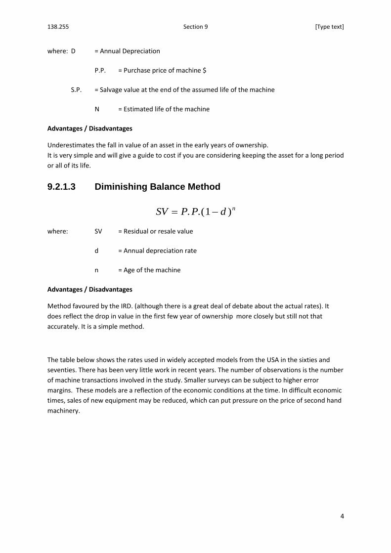
where: D = Annual Depreciation
P.P. = Purchase price of machine $
S.P. = Salvage value at the end of the assumed life of the machine
N = Estimated life of the machine
Advantages / Disadvantages
Underestimates the fall in value of an asset in the early years of ownership.
It is very simple and will give a guide to cost if you are considering keeping the asset for a long period
or all of its life.
9.2.1.3 Diminishing Balance Method
SV P P d n. .( )1
where: SV = Residual or resale value
d = Annual depreciation rate
n = Age of the machine
Advantages / Disadvantages
Method favoured by the IRD. (although there is a great deal of debate about the actual rates). It
does reflect the drop in value in the first few year of ownership more closely but still not that
accurately. It is a simple method.
The table below shows the rates used in widely accepted models from the USA in the sixties and
seventies. There has been very little work in recent years. The number of observations is the number
of machine transactions involved in the study. Smaller surveys can be subject to higher error
margins. These models are a reflection of the economic conditions at the time. In difficult economic
times, sales of new equipment may be reduced, which can put pressure on the price of second hand
machinery.

138.255 Section 9 [Type text]
5
Estimated diminishing balance rates of depreciation. From ASABE Standards.
Category
Estimated depreciation rate
%
Average length of ownership years
Number of observations
Tractor 15 7 712
Combine 15 7 138
Balers 18 7 60
Potato Harvester 21 6 32
Forage Harvester 21 6 62
Sugar Beet Harvester 23 7 27
9.2.1.4 Geometrically adjusted method
Used by ASABE (American Society of Agricultural biological Engineers). It simply adds a first year
correction factor to reflect what happens when new machinery is used.
SV
PPSA SB n*
where: SA = First year correction factor
SB = Annual depreciation factor
Present standard expressed as: RVSV
PP =
Remaining value as a percentage of the original list price at the end of year n.
For
Tractors,
68(0.920)n
Combines, Self propelled windrowers, 64(0.895)n
Balers, Forage harvesters, blowers and self propelled sprayers,
56(0.885)n
All other field machines 60(0.885)n
Advantage: The method that most accurately reflects the reality of the situation.

138.255 Section 9 [Type text]
6
List the possible reasons for the large drop in initial value.
9.2.1.5 Worked Example:
Calculate the value of a $100,000 tractor throughout it’s 10 year life.
Assumptions, straight line method: It will be sold for approximately 10 % of its original purchase
price.
15% for Diminishing balance method. For Geometrically adjusted method, SA = 0.68, SB = 0.920.
Present your results in table format, graph the results.
The IRD’s allowable depreciation rates can be downloaded in a document access through the
following link:
http://www.ird.govt.nz/forms-guides/keyword/businessincometax/ir265-guide-general-
depreciation-rates.html
Both Diminishing Balance and Straight Line rates are illustrated. These can be used as a guide for
business but in some cases the life expectancy of the asset may be rather long and depreciation rate
0
10000
20000
30000
40000
50000
60000
70000
80000
90000
100000
0 2 4 6 8 10
Straight Line Diminishing Balance Adjusted Dim Balance
Year
Trac
tor
Val
ue

138.255 Section 9 [Type text]
7
used low. There is the provision to use a 20% loading but with some specialized machinery this may
not actually depict the true value. An example of this are self propelled forage harvesters. These are
expensive machines used almost entirely by contractors, The problem is that because contractors
require complete reliability from these machines there is no interest in secondhand machines once
the initial 2 to 3 seasons have been completed. Some of the manufacturers have deals where they
will refurbish the machine after 3 seasons in order to maintain reliability. If one of these machines
fail then it can be extremely expensive to repair and most parts are no longer held within New
Zealand, so there can be delays for clients, which is unacceptable. Contractors also use lease options
where they don’t actually own the machine but simply pay a fee for using it. Although these are
high cost machines to run leasing may be best in terms of regular outgoings which makes cashflow
budgeting easier.
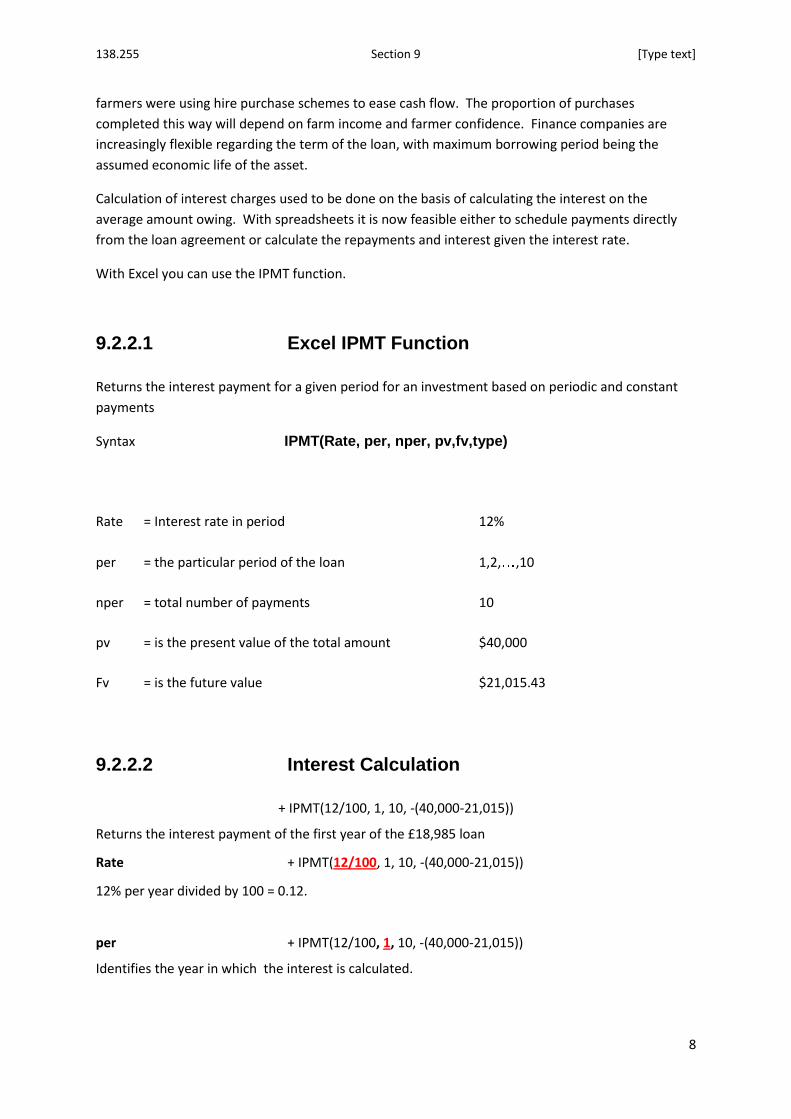
9.2.2 INTEREST ON CAPITAL
Most machinery is purchased using some form of hire purchase agreement.
If a machine is purchased from the company’s own capital, an opportunity cost is charged.
The capital to invest in new machinery is either borrowed or is used from the farmers own capital
reserves. In the latter case an opportunity cost is imposed to account for the loss of income forgone
by using the capital. This situation was becoming increasingly rare as an ever- increasing number of
138.255 Section 9 [Type text]
8
farmers were using hire purchase schemes to ease cash flow. The proportion of purchases
completed this way will depend on farm income and farmer confidence. Finance companies are
increasingly flexible regarding the term of the loan, with maximum borrowing period being the
assumed economic life of the asset.
Calculation of interest charges used to be done on the basis of calculating the interest on the
average amount owing. With spreadsheets it is now feasible either to schedule payments directly
from the loan agreement or calculate the repayments and interest given the interest rate.
With Excel you can use the IPMT function.
9.2.2.1 Excel IPMT Function
Returns the interest payment for a given period for an investment based on periodic and constant
payments
Syntax IPMT(Rate, per, nper, pv,fv,type)
Rate = Interest rate in period 12%
per = the particular period of the loan 1,2, ,10
nper = total number of payments 10
pv = is the present value of the total amount $40,000
Fv = is the future value $21,015.43
9.2.2.2 Interest Calculation
+ IPMT(12/100, 1, 10, -(40,000-21,015))
Returns the interest payment of the first year of the £18,985 loan
Rate + IPMT(12/100, 1, 10, -(40,000-21,015))
12% per year divided by 100 = 0.12.
per + IPMT(12/100, 1, 10, -(40,000-21,015))
Identifies the year in which the interest is calculated.

138.255 Section 9 [Type text]
9
Nper + IPMT(12/100, 1, 10, -(40,000-21,015))
Total period of loan, in this case 10 years.
pv – fv + IPMT(12/100, 1, 10, -(40,000-21,015))
Amount borrowed.
If you are not using a discounted cash flow then omit then insert zero for fv.
A simple spreadsheet can illustrate the procedure.
[a2] Rate [c2] 10%
[a3] nper [c3] 10
[a4] pv [c4] -40,000
[a5] fv [c5] 0
[a7] Year [b7] Interest
[a8] 1 [b8] +IPMT(c$2,a8,c$3,c$4,c$5)
[a9 to 17] should contain years 2 to 10,
[b9] Paste formula from [b8] to [b9 to b17]
The tables should look like:
Interest Calculation
Rate Interest rate charged 8%
nper Total years of loan 10
pv Loan amount -40,000
fv Future value of loan 0
Year Interest
1 $3,200.00
2 $2,979.11
3 $2,740.54
4 $2,482.89
5 $2,204.63
6 $1,904.10
7 $1,579.53
8 $1,229.00
9 $850.43
10 $441.57
Total Interest
$19,611.80

138.255 Section 9 [Type text]
10
9.2.3 Tax Insurance and Housing
These are often simply estimated as a percentage of the purchase price of the machine.
1. Road tax and licensing. Actual costs can be obtained from road licensing and tax.
2. Insurance If machinery is on a hire purchase agreement or financed in any way there may be a requirement to have it insured. A number of specialist insurers will give cover.
3. Housing (assuming it can be allocated) This may not be allocated to general machinery but some specialized machinery may have specific requirements. When running a fleet of machinery it would be wise to make provision for storage but this may be under general expenses rather than allocated to individual machines.
9.3 Machinery Running Costs (Variable Costs)
Variable costs. Costs directly attributable to specific enterprises. The main variable costs
are feeding stuffs (purchased and home-grown), veterinary and medicines, seeds
(purchased and home-grown), fertilisers, sprays and sundry livestock and crop costs.
For the purposes of running costs, our variable costs are:
Fuel and Oil cost
Repair and Maintenance cost
Labour cost
9.3.1 Fuel costs
In practical terms it is very difficult to give an exact figure for fuel consumption.
The fuel consumption of a tractor is governed by the amount of energy demanded at the
drawbar or through the Power Take-off Shaft (PTO).
Individual jobs vary. Tractors operate throughout the year on a range of tasks varying
from heavy duty work such as ploughing or forage harvesting to light chores.
Duty cycles vary within the same job. Even for ploughing, the fuel consumption of an
individual tractor varies considerably over the duty cycle and the average fuel
consumption is only ⅔ of the fuel consumption for peak power.

138.255 Section 9 [Type text]
11
Specific fuel consumption varies. Maximum fuel efficiency is achieved at 90% of
maximum power.
Fuel efficiency varies with engine loading and reaches a maximum at about 90% of
maximum power.
This table, from a study in the US, shows the % of time that a tractor operates at each power level.
The average engine loading throughout the year is 55% of the maximum PTO power of the tractor.
% of time tractors operate at various engine loadings
Engine loading, % of maximum power
Operating time, % of annual use
Over 80 16.8
60-80 23.9
40-60 22.6
20-40 17.5
Under 20 19.2
(Source: Bowers, 1975)
9.3.2 Specific Fuel Consumption
Specific fuel consumption can be given in terms of litres / kWh and is a function of the power
utilisation ratio of the tractor being operated and the power availability. As part of ASAE Standard
S496, the fuel consumption can be calculated from the following equation: (Note: it is part of the
spreadsheet program you do not have to commit to memory)
fc = 2.64Ru + 3.91- 0.203(738Ru + 173)0.5
fc = specific fuel consumption (litres / kWh)
Ru = Power utilisation Ratio
= availablepower PTO
requiredpower PTO
The specific fuel consumption can be calculated while undertaking an individual operation. It may
be used when comparing one’s own machine with hiring an agricultural contractor. In this case
power demand must be calculated also.

138.255 Section 9 [Type text]
12
9.3.3 Fuel Cost
FC = fc * P * pf
where:
FC = $/h
fc = specific fuel consumption l/kWh
P = equivalent PTO power required kW
pf = fuel price (……… $/litre)
The total annual fuel cost can be derived multiplying FC by the annual hours. Estimates of average
annual fuel consumption vary. Estimates range from 70% of the fuel consumption for peak power
from some references down to 40%. Clearly these differences in utilisation may be partly due to the
type of tractors being analysed and hence the work they are required to perform. An analysis from a
survey of tractor tasks according to power for Germany revealed that as power increases the
proportion of time spent on tillage also increases.
9.3.4. Average Annual Fuel Consumption
The average fuel consumption has been approximated from tractor test data. In the US the main
testing station is the Nebraska Tractor Testing Centre which is situated at Nebraska State University.
Website: http://tractortestlab.unl.edu/
Average fuel consumption is approximated as Qavg = 0.305 x P pto
where Qavg is average fuel consumption in L/h
and Ppto is maximum PTO power in kW.
Fuel consumption is clearly dependent on the use of the tractors and machinery. Tractor use in
Germany (Estimation excluding dairy farms) shows the allocation of tractors hour against the engine
power. Larger tractors spend more time on tillage while smaller tractors spend more time on
applying fertiliser and front end loading and other on-farm servicing operation. A similar trend is
likely in New Zealand.

138.255 Section 9 [Type text]
13
(Source: Renius, 1987, 1992)
9.3.5. Typical Fuel Requirements.
Typical fuel requirements for individual field operations is given in this table
Operation Fuel consumption
l/ha
Subsoiling
Ploughing
Heavy cultivation
Light cultivation
Rotary cultivation
Forage harvesting
Combine harvesting
Potato harvesting
15
21
13
8
13
15
11
21
9.3.6. Oil Costs
Oil costs typically represent about 5% of the fuel consumption costs.
Oil consumption is defined as the volume of engine crankcase oil per hour replaced at the
manufacturer’s recommended change intervals.
It is assumed that engine oil is replaced every 200 hours of use. Maybe less in dusty conditions or
when the engine is working at peak load.
OC = Volume of oil every 200 hrs Cost $/litre
0
20
40
60
80
100
120
30 80 130
Sowing, plant protection & cultiv ation,
fertilizing, front end loading, on-farm
operations.A
Vera
ge t
ime p
ort
ion
Rated engine power (kW)
Harv esting
Transport
Tillage

138.255 Section 9 [Type text]
14
9.4 REPAIRS & MAINTENANCE
Repair costs are another important part of machinery costs. The more a machine is used, the
greater is its need for repairs.
However, some machine components have surfaces that rust, rot or otherwise deteriorate over the
years. Repair costs caused by deterioration, though not necessarily affected by the amount of use,
are still considered an operating cost.
The longer agricultural machinery is used, the more repairs are needed to maintain “reliability”.
Reliability is hard to measure with a formula as it expresses the amount of confidence placed in a
machine to perform without an unplanned time loss due to breakdown.
Repair costs should be considered as a necessary and important part of machinery ownership.
Repairs are essential in order to maintain a high level of reliability. Machinery repair costs consist of
the full financial outlay for parts and labour either at the dealers or on the farm. These charges are
in themselves non-standard; labour costs for main dealerships with well equipped workshops are
considerably higher than at a local garage, reflecting the different level of overheads. In addition,
the differences in operator care, in soils, in crops and in climate produce a broad range of repair
costs for similar machines. Ideally, an accurate record of repair and maintenance costs should be
kept for each machine on the farm. As a guide, however, average repair costs are influenced by the
size of the machine, as reflected by its price, and the amount of use.
With the growth in the average size of new tractors and machines, greater productivity is possible.
But this greater productivity means that it is even more important to avoid breakdowns or to be able
to make repairs quickly. Even one hour during periods of critical operations in farming is valuable,
e.g. a breakdown due to a planting delay can lead to yield loss but it is an indirect cost and does not
often feature.
Yield loss cost is probably more important than the direct cost of repairs. Make it a goal, once a
machine is purchased, to provide necessary maintenance and repairs to keep it running at a high
level of reliability.
Listed here are some of the factors affecting repair and maintenance costs:
Repair and maintenance costs are the single most difficult item to predict. There are so many
variable factors:
Work load.
Operator
Inherent machine qualities
Machine age
Operating conditions

138.255 Section 9 [Type text]
15
9.4.1 Sources of R&M costs
With any machine there are 4 main types of repairs:
Routine replacement of wearing parts
Typical examples of routine wear (or replacement) include ploughshares, discs, tine
points, tyres and batteries. Even with the best of care, replacement will be necessary
sooner or later.
But if a rigid maintenance schedule is followed and the equipment or machine is not
abused, an increase or 50% - 100% in parts life can result, depending on the nature of the
part.
Except for excessive abuse, the life of ploughshares, discs and other soil engaging parts is
usually determined by the soil characteristics. Other parts, like tyres and batteries, have
a life that is affected by maintenance and operating environment.
Repair of accidental damage
Machinery accidents can happen even with the best of operators. But carelessness or
rushing a job is far more likely to cause costly accidents. Unfortunately, these types of
accidents often involve a frame, axle, housing or some other part that is hard to replace.
Often these types of parts are not stocked by a dealer, or the total damage to the
machine is quite extensive.
With good management, few, if any, repairs of this nature are needed. Using good
judgement can eliminate most accidental breakage.
Repairs through operator neglect. (Neglecting overhaul and repairs)
Sometimes, the “time” is not taken to perform needed maintenance or minor repairs.
Neglected maintenance and minor repairs almost always lead to more serious problems.
Remember that putting off maintenance and minor repairs can be costly. Use a good
out-of-season repair programme, together with a rigid daily inspection and service
schedule, help avoid expensive repairs.
Routine overhauls
Machines are overhauled to replace worn or defective parts and restore original
performance. Overloading and poor maintenance practices can accelerate these repairs
by 100% or more. Records of repair costs compiled by the Agricultural Engineering
Department of the University of Illinois, in the US, showed that with good management,
repair costs can be reduced by 25% or more. Poor management can raise repair costs
25% above the average.

138.255 Section 9 [Type text]
16
Machinery is becoming more reliable through better quality standards during
manufacture.
Repair & maintenance costs increase towards the end of a machine's life.
The degree to which this happens depends on the complexity of the machine.
There have been a large number of surveys carried out to examine repair and maintenance costs.
Each survey proves one thing: there is a huge amount of variation; but there is certain agreement
regarding the best way to express these costs.
The general method has been to express cumulative repair and maintenance (R&M) costs as a % of
the purchase price of the machine, throughout the life of the machine. In the case of agricultural
tractors economic life is assumed to be between 10K and 12K hours, although some studies have
suggested an economic life as short as 7K hours. Because of the huge variation in the survey data
collected most models should only be used as a “rule of thumb”.
R&M Cost equation takes the general form:
TAR = Rf1(X)Rf2
Where TAR = Total Accumulated Repair costs expressed as a percentage of the purchase price
X = Accumulated hours / 1000
Rf1, Rf2, = Repair cost coefficients.
The ASAE has published a number of models in editions of the ASAE Yearbook. Most models have
followed the from of the above equation but the values of coefficients Rc1 & Rc2 have changed as
more data has become available and a newer generation of tractors is surveyed and the result has
been a reduction in expected R&M costs when expressed as a percentage of purchase price. This is
due increased reliability and quality of machine and better machinery management on farms in
some instances, or a combination of both.
9.4.2 Annual R&M Costs
Example calculation
A $100,000 tractor operates for 800 hours per year.
Rf1 = 0.007, Rf2 = 2
What are the accumulated R&M costs after 7 years?
TAR = 0.07(5600/1000)2
= 0.219 of initial purchase price

138.255 Section 9 [Type text]
17
= 0.219 100,000
= $21,900
Repair costs in year 7 = (Accumulated costs in year 7) minus (accumulated costs in year 6)
Cost after 6 years:
TAR = 0.007(4800/1000)2
= $16,128
Repair cost in year 7 = 21,900 - 16,128
= $5,772
Annual R&M Charges (800 hours of annual use)
Cumulative R&M Costs
$
$
0
2000
4000
6000
8000
10000
1 2 3 4 5 6 7 8 9 10YEAR
0
10000
20000
30000
40000
50000
1 2 3 4 5 6 7 8 9 10
YEAR
138.255 Section 9 [Type text]
18
9.5 LABOUR COSTS
Labour charge for machinery operations
= operator’s hourly rate (£) time required (hr)
Operator’s hourly rate should include
National Insurance
employer’s liability insurance
overtime
any other benefits
The labour charge for machinery operations costs are simply calculated by multiplying the operator’s
hourly rate by the time required. The operator’s hourly rate should include NI, employer’s liability
insurance, overtime and any other benefits.
This calculation for the labour charge infers that labour is available by the hour, on a casual basis,
whereas the real value of labour at the time for which it is required may be considerably higher
because of its opportunity cost. It may be necessary, e.g. to hire permanent staff to ensure their
availability at a critical time of the year. In such circumstances, the annual cost is more appropriate
than the hourly labour cost. Provided that this aspect of labour availability is borne in mind, the
hourly labour charge is an important component of machinery operating costs for systems
comparisons at the enterprise level.
9.6 PUTTING IT ALL TOGETHER
The operating costs of a tractor can be calculated by including:
Depreciation
Interest on Capital
Tax & Insurance
Repairs & Maintenance
Fuel & Oil
Labour

138.255 Section 9 [Type text]
19
9.6.1 SPREADSHEET EXAMPLE
Tractor Operating Costs per hour
When considering average operating cost, in this example, minimum cost in year 6.
Considering discount has a major effect as figures are based on list price.
Inflation has not been considered.
No account taken of extra inconvenience due to additional breakdown.
Economics should not be the only consideration.
9.7 Fleet Management
9.7.1 Two main tasks for machinery manager:
1) Calculate the optimum fleet for their needs.
2) Calculate the best replacement policy for individual machines.
Each part of the system will have it’s own issues to resolve, for example in terms of tractor selection
three stages could be considered:
Maximum tractor power demand
Tractor fleet size
Tractor power mix
10
20
30
1 2 3 4 5 6 7 8 9 10
Co
st/
h
Year
Av.
Annual

138.255 Section 9 [Type text]
20
State the main factors governing the above:
1)
2)
3)
The problem of selecting tractor power seems to dominate thinking and usually approached as being
an intuitive process. The problem with relying on intuition is that it is based on managerial
experience, takes years to learn and it is not readily transportable to other problems or scenarios.
Analytical procedures are now available to obtain a more accurate estimate of tractive performance
from particular soils, weather and tyre data can be used to predict machinery requirements.
9.7.2 TIME FRAME:
Most machinery assets have a life of 10 - 15 years, therefore there is a need for long term
planning.
It is not always possible to implement plans immediately, but the manager must always have
long term goals.
To ensure a reasonable degree of efficiency in mechanisation management over a long period it is
essential to have a long term plan for replacement of major capital items. It is best to try and spread
replacement fairly evenly even though machines will have different replacement periods.
Planning difficulties:
Farming, horticulture and forestry are subject to greater variability than other businesses,
State some of the sources of variability in these businesses:
9.7.3 RECENT RESPONSES TO CHANGE:
Changing cropping pattern in order to maximise the production of profitable crops.
Simplifying the machinery system required to service the range of crops grown.
Continued increase in farm size to achieve economies of scale.
Use of contractors, machinery rings and machinery hire to reduce capital investment.
138.255 Section 9 [Type text]
21
9.7.4 ACHIEVING A BALANCE
Optimum machinery management is achieved when the overall profitability of the farm is
maximised. This economic goal is not necessarily the equivalent to minimising machinery costs for a
number of reasons.
Over mechanisation: Higher costs particularly fixed costs.
Under mechanisation: Physical requirements of the farm are not met. Financial
performance deteriorates.
As mentioned previously margins in agriculture have tended to decline in the long term.
Implications for mechanisation planning are clear. When setting up a mechanised system the whole
farm needs to be examined and maybe changed. A further response has been greater specialisation
leading to major changes in work patterns.
9.7.5 CHANGES IN WORK PATTERN
Desired change in an economic sense can cause other difficulties, concentration of work
pattern is a particular problem for cropping systems. For example in Europe
In trying to improve economic performance farmers have increasingly specialised in one
crop or one crop group. For example winter wheat is being grown more and more at the
expense of spring cereals but this has led to an increased concentration in work load.
Consequences of this are:
A larger percentage of the farm is dealt with using one machinery set.
Increased timeliness pressure because of the predominance of one cropping pattern.
These two factors make it more difficult to maximise the utilisation of resources such as machinery.
9.7.6 EFFECT OF FARM SIZE
List some of the effects of farm size
Larger farms have been more successful at reducing mechanisation costs
State possible reasons for this:

138.255 Section 9 [Type text]
22
9.8 REFERENCE MATERIALS:
Available in the library:
Lincoln University, Financial Budget Management 2002
Choosing and using Farm Machinery. Brian Witney.
Read the farm machinery sections in some of the following:
Farmers Weekly
Power Farming
Rural news, etc. etc.

138.255 Section 9 [Type text]
23