Embed Size (px)
Citation preview
ANIPLA COMPUTER VISION 2012
Milano - June 14th, 2012
MACHINE VISION BENCHMARKING
S. Giardino – F. Gori – C. Salati Consorzio T3LAB, via Sario Bassanelli 9/11, 40137 Bologna
[email protected] – [email protected] – [email protected]
Abstract
The VIALAB benchmark project aims at comparing and evaluating commercial machine vision libraries, and in particular those that are more widely used by the automation industry in Emilia-Romagna Region. Typical industrial applications of machine vision have inspired different challenges by means of which commercial toolkits will be evaluated. Each challenge consists of a description document and a common benchmark framework that invokes specific library functions. The sets of images that will be used for the evaluation have been completely acquired and synthetically produced by VIALAB. Results will be made public at the end of the project (November 2012).
Keywords
Machine Vision, Benchmark, Library, Metrics
1 INTRODUCTION
1.1 Yet another benchmark?
The “machine vision benchmark” that is part of the VIALAB project [1] is different from academic benchmarks in that it is specifically aimed at commercial libraries and their overall characteristics: its goal is to support users in the selection of the software that best fits their needs.
The VIALAB benchmark shares similar motivations with [2]: “The intention of any machine vision benchmark should be to bring more transparency into the market for vision software and vision systems. Such a benchmark should enable users of vision systems to determine more easily which software is most suitable for the requirements of a given application”.
2
All library suppliers do certainly perform product comparisons, and they also provide information to the general public. But there may be no guarantee that this information is not biased, even without malice, just because it may be related to datasets for which the behavior of the library has been optimized.
In fact users are surrounded by conflicting information. Not only, even if they weren’t conflicting, the information sources would not be comparable: they would be related to different datasets and different computing platforms.
What the VIALAB benchmark is aiming at is the construction of an independent benchmark, based on an independent dataset, and the provision of information that is unbiased and comparable. We want to compare some of the most relevant, commercial machine vision libraries, and beside them the open source, BSD licensed OpenCV [4], but we are open to consider any additional libraries that adhere to the rules of the benchmark.
The commercial libraries we are currently considering are: • Cognex VisionPro • Matrox MIL • MVTec Halcon • Teledyne/DALSA Sapera
This list comes from a survey that we have performed among companies that use machine vision in the Emilia-Romagna Region [7][8], vendors, integrators, OEM, final users.
Additionally, we think that nowadays, because of its widespread use and its generally perceived quality level, OpenCV plays a most important role in machine vision. Our perception has actually been confirmed by the outcomes of the survey [7][8], which shows that several participating companies are using OpenCV in one way or another, sometime in conjunction with a commercial library. As a consequence, we think that OpenCV is a baseline against which all commercial libraries should compare themselves.
Even though execution time is not the only metric of a benchmark, and in particular of the VIALAB benchmark, it is definitely a relevant metric and one that it is difficult to make really comparable: because we think that comparability of results is essential, unlike [2] we will require the computing platform to be the same for all libraries, and in order to guarantee this we ourselves will run the tests for all libraries on our own platforms. We will actually define a set of reference platforms, and we will keep it evolving to follow the developments of the technology (see sections 2.3.2 and 2.4).
Not only computing technology evolves, libraries do too, and we want to be ready to follow their evolution. We want also to be able to allow other libraries to join the benchmark: this means that tests must be easily repeatable. In order to make this possible, even when they are related to evaluation of positions in world-coordinates, they must still be based on a dataset of images: it will be the associated ground truth that relates them to the world-coordinates 1.
1.2 A collaborative strategy
We will run the benchmark as part of the VIALAB project, but we think that the best way we can run it is in cooperation with library suppliers. The reasons for this are manifold:
1 "Ground truth" is used in the scientific vernacular to refer to the presumed objective reality of a statement or situation, in contrast with some predicted or computed expectation of reality. "Is (x) ground truth?" is a way of asking "Is x really what is going on, objectively, versus some evidential claims we are making?" Ground truthing (verb) in science is gathering objective data to assess whether a theoretical model is accurate. [4]
3
among others and most relevant is that each library supplier is likely the best user of its own toolkit, and we would like to compare the best possible solutions for each of the challenges of the benchmark.
Therefore, whenever possible, we want to run our benchmark in cooperation with library suppliers. In practice, toolkit suppliers will be invited to provide their solutions to the challenges that are part of the benchmark: these solutions, which must agree with a prototype that we provide, will then be plugged in our engine, that will take care of collecting all metrics information that we define as relevant for that challenge.2
The results of the benchmark will “include the code fragment used to solve the benchmark task. Beside transparency, this will allow users to learn more about the use of a given system” [2].
In fact, we expect that cooperation with library suppliers can go much further than what indicated above. What we would additionally expect includes: • Review of the general methodology and of each challenge we propose, and proposals for
their improvement. • Contributions to the creation of a common dataset.
While our benchmark was generated to answer a need that was clearly perceived among users, and while we recognize that contributing to it has a cost for library suppliers, we think that it can go to their benefit too: “The Middlebury Stereo Dataset and the NIST Face Recognition Grand Challenge have succeeded well in advancing their respective research algorithms by providing well-defined challenge tasks with ground truth and evaluation metrics” [3].
1.3 Functionalities vs. operators
[2] states that “the aim of … a benchmark should not be to compare single methods such as the execution time of a Sobel filter but to evaluate how well an application can be solved with the software”.
This is also our general understanding and, based on preliminary contacts we have had with suppliers, there seems to be a consensus among them about this.
This doesn’t mean that one has to consider only specific application cases as a whole. Consider for example the problem of object localization in world coordinates: solving this problem implies that camera calibration and object detection and localization in the image space are also performed. Camera calibration could thus be considered only as an operator that must be evaluated as part of complete functionalities. However, due to its complexity and the relevance it has for several different applications we think that the characteristics of camera calibration are worth being assessed on their own. A similar argument can be made for object detection and localization in the image space.
1.4 Synthetic images
Synthetic images are an accepted practice in the scientific community (e.g. [14], [15]). [14], in particular, states: “… to use synthetic images, where ground truth is known by design. Paradoxically, such synthetic image sets may in many ways be more natural than an arbitrary collection of ostensibly “natural” photographs, because, for a fixed number of images, they
2 As previously indicated, it is part of the VIALAB project to perform a benchmark of commercial libraries that are most relevant in Regione Emilia-Romagna. For these libraries, in case the supplier doesn’t provide a solution VIALAB will take care of implementing one, guaranteeing a best effort approach.
4
better span the range of possible image transformations observed in the real world. The synthetic image approach obviates labor-intensive and error-prone labeling procedures, and can be easily used to isolate performance on different components of the task. Such an approach also has the advantage that it can be parametrically made more difficult as needed (e.g., when a given model has achieved the ability to tolerate a certain amount of variation, a new instantiation of the test set with greater variation can be generated). Given the difficulty of real-world object recognition, this ability to gradually ‘ratchet’ task difficulty, while still engaging the core computational problem, may provide invaluable guidance of computational efforts.”
Based on these arguments we have applied synthetic techniques widely, both in the creation of images with a ground truth that is known a priori and in the introduction of controlled nuisances.
2 STRUCTURE OF THE BENCHMARK
2.1 General organization
The benchmark will be organized as a set of challenges, each addressing a specific functionality and each independent from the others.
Each challenge will have its own definition, even though all definitions will follow the same pattern (see section 3.1).
Each challenge will be run according to the same protocol (see section 3.2).
2.2 The role of OpenCV
In our benchmark, OpenCV is not only the baseline against which all commercial libraries will be compared, it plays also two other roles: • It is the toolkit that we will use for the construction of the benchmark engine (the program
that invokes the library specific procedures that solve the challenges we propose, collects the results and computes the performance metrics we are interested in).
• It is the toolkit for which we are going to develop prototype challenge solutions that we will use during the design of a challenge and that we will provide to the library suppliers to help them design their own solutions.
These prototype solutions will additionally be used for the characterization of OpenCV as a toolkit.
2.3 Which metrics?
Two questions have to be asked about the way we measure the characteristics of machine vision libraries: • What do we want to measure? • How do we measure what we want to measure?
The second question has a set of technical implications that will be dealt with on a case by case basis. Example are given by the challenges that have already been defined [5].
The first question is more related to a strategic decision but in any case, if we decide that a characteristic of libraries is so relevant for users that it is worth being measured, we should indicate a way of measuring it.
5
Following is a list of characteristics that we have addressed; not necessarily all of them apply to all functionalities that we consider: those that apply will be indicated on a case by case basis
2.3.1 Completeness of functionalities
This is certainly something users are interested in, and it is something we have tried to address in our survey [7]; however, it is also something that cannot be easily measured.
Different libraries may support different sets of functionalities and assigning a consistent value to different functionalities is not possible. Additionally, a library may have marketing related reasons not to support a functionality, or not to support it directly. Therefore we will not deal with this issue explicitly.
However, when we decide that we want to test a function it may well be that a library will result as not supporting it: this has happened for our first challenge, “camera calibration”.
A supplier has declined to participate to this first challenge because its library doesn’t support this function, though in principle it has declared it is willing to take part to the benchmark. If, in future, this supplier will actually join our project when other functionalities are addressed the fact that it hasn’t taken part to the “camera calibration” challenge will be registered.
2.3.2 Efficiency (Speed)
Our benchmark will not be focused only on speed, though speed is a significant feature of a library. Based on what we have stated above, we will not consider the execution time of individual operators, but instead that of complete functions.
However, speed may depend significantly on the computing platform we are considering and the relative performance of two libraries may vary a lot when we consider different platforms.
In order to assess speed consistently for all libraries we will test them on the same set of computing platforms and this set will be defined so as to be significant and representative of different types of applications: standard PC and embedded computers, single core and multi-core, with or without GPU acceleration.
Not necessarily all libraries will even support all platforms, but this fact is itself considered a significant evaluation criterion for users.
Time will normally be measured as “watch time”, having guaranteed and verified that no significant disturbances affect the measured value.
Time of day will be captured with the granularity of milliseconds based on the Unix-like function
struct timeval { time_t tv_sec; // seconds suseconds_t tv_usec; // microseconds }; int gettimeofday(struct timeval *tv, struct timezone *tz); that has been implemented on Windows based on the following reference http://suacommunity.com/dictionary/gettimeofday-entry.php and that we call with tz==NULL.
Note that the above function allows to capture time with the granularity of microseconds, but Windows Vista systems have a native granularity of milliseconds which we are limited to.
6
In order to allow the benchmark engine to measure the execution time of each relevant section of a solution, solutions will be required to be structured according to a template that will be part of each challenge definition, when relevant.
The execution time of a section is obtained by measuring the time taken by the repeated execution of such section for N times and then dividing by N, getting a mean value. N is chosen large enough so that we are able to measure time with higher resolution than what is offered by gettimeofday function.
In the organization of the challenge execution we will take care to avoid most circumstances that can introduce unpredictable effects in the efficiency measure: • When we submit the images of the dataset to the solution, we will avoid that the images of
two consecutive test cases are mutually related, e.g.: in a object detection task the model objects will be different in the two test cases, the target objects will be in a different pose in the two test cases.
• This will also avoid that the content of the memory cash is significant at the beginning of a test set.
• The “warming up” time, due to the code that has to be brought in main memory by the operating system prior to execution, is not included in our time measurement, as the measurement starts after the first execution.
Not always execution time, as defined above, is particularly significant. If we consider camera calibration as a complete function, computer execution time is only a part of it, and other factors are more significant. In this case the number of images that are necessary to accurately carry out the procedure is probably a better index.
2.3.3 Ease of use
Ease of use is reasonably related to the complexity of a solution. In turn, this is reasonably related to several characteristics of the piece of code that implements the solution (once it has been cleared of its data marshaling section and of other structural sections): • Overall number of statements • Number of calls to library functions • Number of atomic parameters of each call3 • Cardinality of the domain of each parameter.
There are 2 difficulties here: • How to do this counting? • What is the function that relates these numbers to the complexity of the solution?
In order to avoid these difficulties a different approach has been taken, thus to consider a general purpose SW complexity metrics: the Halstead complexity [9][10][11] metrics looks most appropriate for our purpose since it takes into account most of the complexity indices we have indicated.
Additionally, it is supported by several SW tools, and based on it several secondary indices have also been defined [9].
3 Even if a parameter allows a default value, the presence of a parameter represents intrinsically a complexity factor. When can we use the default value, and when a different value is more appropriate? The possibility of using a default value may reduce the contribution of a parameter to the complexity of the solution but does not nullify this contribution.
7
2.3.4 Interoperability
Because of the special role that OpenCV plays in the machine vision community, and because OpenCV is neutral w.r.t. commercial libraries, all challenges will define APIs that are based on data structures that are typical of OpenCV.
Though interoperability is likely to be considered a secondary metrics, we think that the most likely hybrid situation that application developers will face is that of using their own proprietary SW solutions in combination with commercial libraries. It is often the case that chunks of OpenCV SW have been incorporated in proprietary solutions [7], so it is not unlikely that proprietary solutions take OpenCV data structures into account.
Additionally, OpenCV is widely used in academic institutions, so that many developers are accustomed to it and may wish to use it in combination with commercial libraries.
Interoperability of a commercial library will thus be measured in terms of ease and efficiency of use of OpenCV data structures in the implementation of solutions.
Each solution is expected to start with the marshaling of the data structures it has received in input so that they fit its intrinsic needs. #include <time.h> . . . time_t tStamp0, tStamp1, . . .; . . . outputParameters f(inputParameters) { tStamp0 = time(NULL);
// data marshaling to be implemented as an external // procedure in a separate file
Data marshaling(); // just a place holder tStamp1 = time(NULL); . . . }
Ease of use will be measured according to the metrics defined in section 2.3.3, while interoperability will be measured as the time it takes for marshaling, (tStamp1-tStamp0) in the example above.
2.3.5 Effectiveness of object detection
The performance of object detection tasks is evaluated by using the typical approach of receiver operating characteristic (ROC) analysis.
Object detection algorithms are treated as binary classifier systems: ROC curves are created by plotting the fraction of true positives out of the positives (TPR = true positive rate) vs. the fraction of false positives out of the negatives (FPR = false positive rate), at various detection threshold settings (TPR is also known as sensitivity, and FPR is one minus the specificity or true negative rate) [12].
The Area Under Curve (AUC) is eventually considered for the assessment of algorithms: it is equal to the probability that a classifier will rank a randomly chosen positive instance higher than a randomly chosen negative one (assuming “positive” ranks higher than “negative”) [12].
Object detection is performed looking for a set of models in a dataset of images. The objects of the set have been selected because they have been deemed representative of those
that are relevant for industrial applicationstexture and objects with little instances as well as multiple instances of objects.
2.3.6 Accuracy and precision
The following concepts will be considered throughout the benchmark while assessing object localization algorithms:• Accuracy of measurement (accuracy):
quantity value and a true quantity value of a measurand.• Trueness of measurement (trueness):
infinite number of replicate measured quantity v• Measurement precision (precision):
measured quantity values obtained by replicate measurements on the same or similar objects under specified conditions.
Trueness and precision concepts will be used as evaluation metrics.Measurement precision is usually expressed
such as standard deviation, variance, or coeof measurement [13].
Measurement trueness is not a quantity andbut a measure for closeness of agreement isnumber of replicate measured quantity
Please note that in our benchmark ttrueness concept.
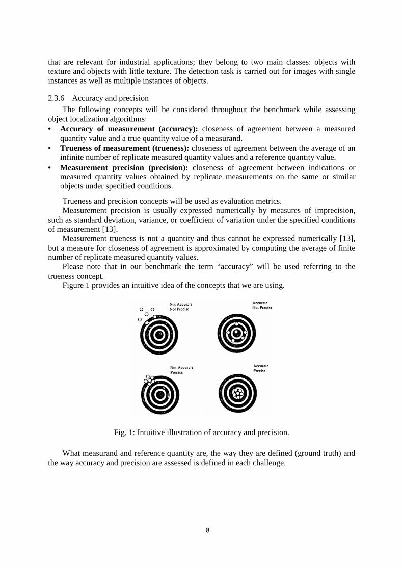
Figure 1 provides an intuitive idea of the concepts
Fig. 1: Intuitive illustration of accuracy and precision.
What measurand and reference quantitythe way accuracy and precision are assessed is defined in each challenge.
8
industrial applications; they belong to two main cla texture. The detection task is carried out for images with single
instances as well as multiple instances of objects.
and precision
The following concepts will be considered throughout the benchmark while assessing object localization algorithms:
measurement (accuracy): closeness of agreement between a measured quantity value and a true quantity value of a measurand. Trueness of measurement (trueness): closeness of agreement between the average of an infinite number of replicate measured quantity values and a reference quantity value.Measurement precision (precision): closeness of agreement between indications or measured quantity values obtained by replicate measurements on the same or similar objects under specified conditions.
sion concepts will be used as evaluation metrics. precision is usually expressed numerically by measures o
deviation, variance, or coefficient of variation under the specified conditions
rement trueness is not a quantity and thus cannot be expressed numericallybut a measure for closeness of agreement is approximated by computing the number of replicate measured quantity values.
Please note that in our benchmark the term “accuracy” will be used referring to the
provides an intuitive idea of the concepts that we are using.
: Intuitive illustration of accuracy and precision.
reference quantity are, the way they are defined (ground and precision are assessed is defined in each challenge.
belong to two main classes: objects with for images with single
The following concepts will be considered throughout the benchmark while assessing
closeness of agreement between a measured
closeness of agreement between the average of an alues and a reference quantity value.
closeness of agreement between indications or measured quantity values obtained by replicate measurements on the same or similar
numerically by measures of imprecision, specified conditions
d numerically [13], approximated by computing the average of finite
” will be used referring to the
are, the way they are defined (ground truth) and
2.3.7 Robustness
Nuisance factors are gradually introduced into images, from low to high levels, for a total of N levels, defined in each challenge,into images synthetically, each of them independently of the others.
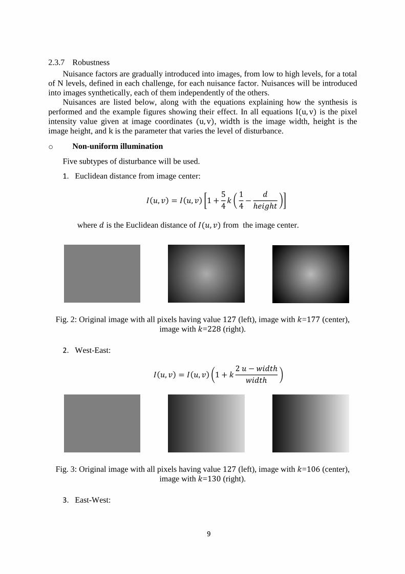
Nuisances are listed below, along with the equations explaining how the synthesis is performed and the example figures sintensity value given at image coordinates image height, and k is the parameter that varies the level of disturbance.
o Non-uniform illumination
Five subtypes of disturbance will be used.
1. Euclidean distance from image center:
�
where � is the Euclidean distance of
Fig. 2: Original image with all pixels having value
2. West-East:
Fig. 3: Original image with all pixels having value
3. East-West:
9
Nuisance factors are gradually introduced into images, from low to high levels, for a total challenge, for each nuisance factor. Nuisances will be introduced
into images synthetically, each of them independently of the others. Nuisances are listed below, along with the equations explaining how the synthesis is
performed and the example figures showing their effect. In all equations intensity value given at image coordinates �u, v�, width is the image width,
is the parameter that varies the level of disturbance.
uniform illumination
types of disturbance will be used.
Euclidean distance from image center:
���, �� � ���, �� �1 � 54 � � 14 � �
������ �
is the Euclidean distance of ���, �� from the image center.
: Original image with all pixels having value 127 (left), image with image with �=228 (right).
���, �� � ���, �� �1 � � 2 � � $����$���� �
: Original image with all pixels having value 127 (left), image with image with �=130 (right).
Nuisance factors are gradually introduced into images, from low to high levels, for a total for each nuisance factor. Nuisances will be introduced
Nuisances are listed below, along with the equations explaining how the synthesis is howing their effect. In all equations I�u, v� is the pixel
is the image width, height is the
from the image center.
(left), image with �=177 (center),
(left), image with �=106 (center),
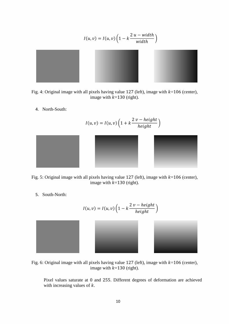
Fig. 4: Original image with all pixels having value
4. North-South:
Fig. 5: Original image with all pixels having value
5. South-North:
Fig. 6: Original image with all pixels having value
Pixel values saturate at with increasing values of
10
���, �� � ���, �� �1 � � 2 � � $����$���� �
: Original image with all pixels having value 127 (left), image with image with �=130 (right).
���, �� � ���, �� �1 � � 2 � � ������������ �
: Original image with all pixels having value 127 (left), image with image with �=130 (right).
���, �� � ���, �� �1 � � 2 � � ������������ �
: Original image with all pixels having value 127 (left), image with image with �=130 (right).
Pixel values saturate at 0 and 255. Different degrees of deformation are achieved with increasing values of �.
(left), image with �=106 (center),
(left), image with �=106 (center),
(left), image with �=106 (center),
. Different degrees of deformation are achieved
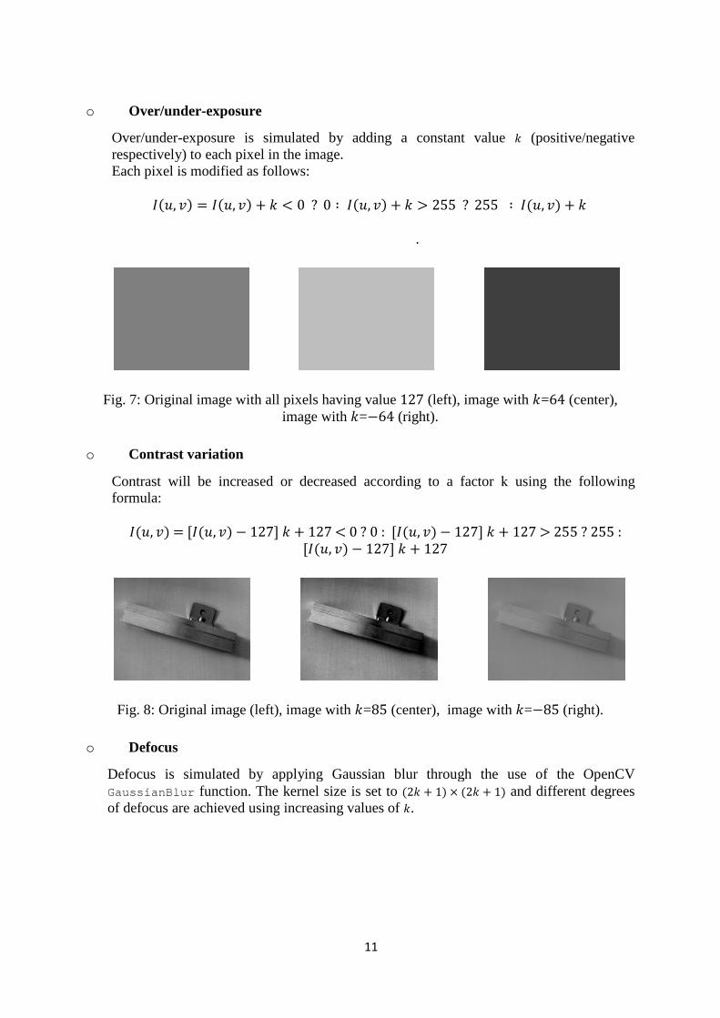
o Over/under-exposure
Over/under-exposure is simulated by adding a constant value respectively) to each pixel in the image.Each pixel is modified as follows:
���, �� � ���, �� �
Fig. 7: Original image with all pixels having value
o Contrast variation
Contrast will be increased or decreased according to a factor formula:
���, �� � [���, �� � 127]
Fig. 8: Original image (left), image with
o Defocus
Defocus is simulated by applying Gaussian blur through the use of the OpenCV GaussianBlur function. The kernel size is set to of defocus are achieved using
11
exposure
exposure is simulated by adding a constant value �
respectively) to each pixel in the image. Each pixel is modified as follows:
� � � - 0 ? 0 / ���, �� � � 0 255 ? 255 / �
.
: Original image with all pixels having value 127 (left), image with image with �=�64 (right).
Contrast will be increased or decreased according to a factor k using the following
127] � � 127 - 0 ? 0 : [���, �� � 127] � � 127 0 255 ? 255 :
[���, �� � 127] � � 127
: Original image (left), image with �=85 (center), image with �
Defocus is simulated by applying Gaussian blur through the use of the OpenCV function. The kernel size is set to �2� � 1� 3 �2� � 1� and different degrees
of defocus are achieved using increasing values of �.
� (positive/negative
���, �� � �
(left), image with �=64 (center),
using the following
� 127 0 255 ? 255 :
�=�85 (right).
Defocus is simulated by applying Gaussian blur through the use of the OpenCV and different degrees
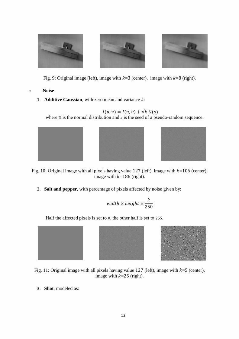
Fig. 9: Original image (left), image with
o Noise
1. Additive Gaussian, with zero mean and variance
where 4 is the normal distribution and
Fig. 10: Original image with all pixels having value
2. Salt and pepper, with percentage of pixels affected by noise given by:
Half the affected pixels is set to
Fig. 11: Original image with all pixels having value
3. Shot, modeled as:
12
: Original image (left), image with �=3 (center), image with
, with zero mean and variance �:
���, �� � ���, �� � √� 4�6� is the normal distribution and 6 is the seed of a pseudo-random sequence.
: Original image with all pixels having value 127 (left), image with image with �=186 (right).
, with percentage of pixels affected by noise given by:
$���� 3 ������ 3 �250
the affected pixels is set to 0, the other half is set to 255.
: Original image with all pixels having value 127 (left), image with image with �=25 (right).
(center), image with �=8 (right).
random sequence.
(left), image with �=106 (center),
, with percentage of pixels affected by noise given by:
(left), image with �=5 (center),
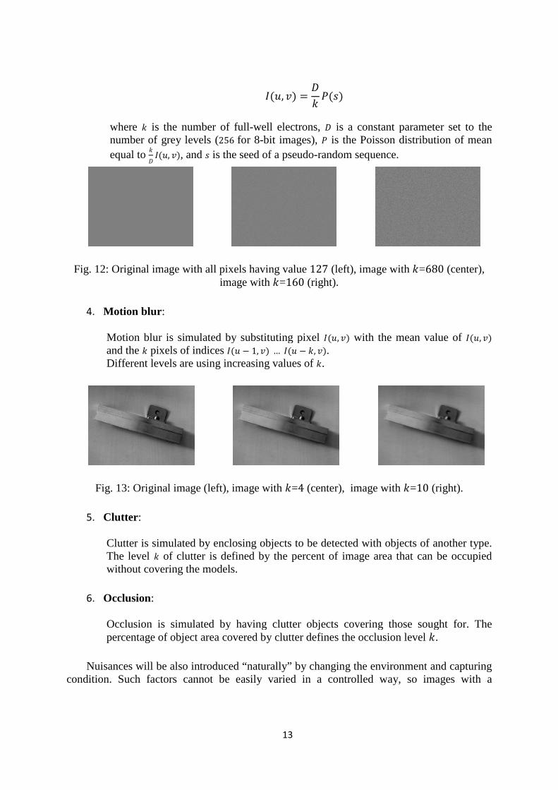
where � is the number of fullnumber of grey levels (equal to �7 ���, ��, and
Fig. 12: Original image with all pixels having value
4. Motion blur: Motion blur is simulated by substituting pixel and the � pixels of indices Different levels are using
Fig. 13: Original image (left), image with
5. Clutter: Clutter is simulated by enclosing objects to be detected with objects of another type. The level � of clutter is defined by the percent of image area that can be occupied without covering the models.
6. Occlusion: Occlusion is simulated by having clutter obpercentage of object area covered by clutter defines the occlusion level
Nuisances will be also introduced “naturally” by changing the condition. Such factors cannot be easily varied in a c
13
���, �� � 7� 8�6�
is the number of full-well electrons, 7 is a constant parameter set to the number of grey levels (256 for 8-bit images), 8 is the Poisson distribution of mean
, and 6 is the seed of a pseudo-random sequence.
: Original image with all pixels having value 127 (left), image with image with �=160 (right).
Motion blur is simulated by substituting pixel ���, �� with the mean value of pixels of indices ��� � 1, �� … ��� � �, ��.
Different levels are using increasing values of �.
: Original image (left), image with �=4 (center), image with �
Clutter is simulated by enclosing objects to be detected with objects of another type. of clutter is defined by the percent of image area that can be occupied
without covering the models.
Occlusion is simulated by having clutter objects covering those sought for. The percentage of object area covered by clutter defines the occlusion level
Nuisances will be also introduced “naturally” by changing the environmentcondition. Such factors cannot be easily varied in a controlled way, so images with a
is a constant parameter set to the is the Poisson distribution of mean
(left), image with �=680 (center),
with the mean value of ���, ��
�=10 (right).
Clutter is simulated by enclosing objects to be detected with objects of another type. of clutter is defined by the percent of image area that can be occupied
jects covering those sought for. The percentage of object area covered by clutter defines the occlusion level �.
environment and capturing ontrolled way, so images with a
14
significant level of natural nuisances will not be subjected to synthetic changes and the amount of nuisances will be given in nominal levels: low, medium, and high nuisance.
2.4 Evaluation platforms
Several different execution platforms have been envisioned for our benchmark. Due to resource constraints we have finally decided to consider a single platform: a PC, with a quad-core Intel i7-950 CPU running at 3.07GHz, equipped with an NVIDIA GeForce GTX460 graphic card, with 336 cores, 1GB of video RAM and a bandwidth of 115.5GB/s, with Windows 7 64 bit.
The choice of Windows is related to the development environment that we have selected for the framework, Visual Studio.
This platform will support tests with three very different configurations: • single processor, • symmetric multi processor, • symmetric multi processor with GPU HW acceleration.
Simple embedded platforms, ARM based platforms and Linux could unfortunately not be considered.
3 CHALLENGES
3.1 Description of a challenge
Each challenge will be described according to the following pattern, where each point corresponds to a section of the definition:
1. General definition The functionality that is evaluated and the metrics that are applied are described in this section. These metrics are generally specific instances of those that are defined in this document in the following parameters.
2. Main parameters This section defines several facets of the challenge and the conditions under which the metrics indicated are computed:
• The conditions under which dataset images are created, including the characteristics of cameras and optics and whether images are real or synthetic.
• The nuisances that may affect the images of the dataset and the degree they may have. In order to introduce nuisances in a calibrated form we will normally resort to synthetic images, but images with non calibrated real nuisances are also possible in the dataset. The algorithm for the injection of nuisances will also be described and so the extent to which injection will take place.
• The parameters and deformations that are considered and the values they can have.
3. Component tasks This is the part which defines the procedures that are used to perform the assessment and the theory behind the choice of them.
4. Dataset and ground truth This section explains how the evaluation dataset is organized and in which way the ground truth was created in order to have it as accurate as possible.
15
5. Evaluation metrics This part describes how the results computed by a library are compared against the ground truth and how the comparison data are then summarized to show the final results.
6. Task interface This section defines the API of the challenge, thus the API that must be implemented based on the library of a vendor. This API is defined as a C header file, with the semantics of each function described both in the text of this section and in the header file. When relevant, a template of each function will be provided, together with the API. The template, that should be completed by each solution, is meant to identify and separate the different sections of code that comprise a solution, but that should be kept separate from the standpoint of SW metrics. A typical template, where 3 different sections of the solution have been highlighted, and where these sections have been separated by timestamps that allow to measure the time of their execution, may look as follows:
#include <time.h> . . . time_t tStamp0, tStamp1, tStamp2, tStamp3; . . . outputParameters f(inputParameters) { tStamp0 = time(NULL); // data marshaling to be implemented as an external // procedure in a separate file Data marshaling(); // just a place holder tStamp1 = time(NULL); // training to be implemented as an external procedure // in a separate file Training(); // just a place holder tStamp2 = time(NULL); // the object detection code is the core of the solution. // It should all be contained in this file Detection(); // just a place holder tStamp3 = time(NULL); }
The data structures that represent an image in this API are those defined by OpenCV. As a complement of this API definition two other C implementation files are attached: • An example solution of the challenge, thus an implementation of the API, based on
OpenCV. • The benchmark framework (C program) that invokes the API.
Finally a development dataset will also be made available as part of the challenge definition. Notice that not all the evaluation dataset will be available for development: this is because we want solutions to be general, to be capable to handle a class of problems, e.g. “detection of non-textured” objects, and not only a list of specific cases.
16
3.2 Challenge execution protocol
The following protocol will be followed in the execution of each challenge:
1. VIALAB distributes a draft definition of the challenge to all library vendors. This definition includes: • A deadline for the comments that VIALAB expects to receive from library vendors4. • An estimate of the effort (person-days) that is necessary to a library vendor for the
implementation of the solution of the challenge (based on the time it took VIALAB to implement the prototype solution with OpenCV).
2. VIALAB waits for comments from library vendors. Comments should include the time that participants deem necessary for the implementation of the solution of the challenge.
3. VIALAB distributes a revised definition of the challenge, including a deadline for the solutions to be provided by library vendors (based on their comments).
4. VIALAB waits for solutions from library vendors. 5. VIALAB runs solutions on the test-bench and on the challenge dataset. 6. VIALAB discusses individual results with participating vendors. The discussion will
include sharing information about the specific results of the vendor and the average results. This discussion is meant to make sure that no unreasonable results are made public due to misunderstandings or errors.
7. All results are published.
The description of each challenge will be circulated for comments among all library vendors that have been invited to participate to the benchmark, independent of the fact that they have accepted and of the fact that VIALAB will implement a solution for challenge based on their library.
4 AN EXAMPLE OF CHALLENGE: THE CALIBRATION CHALLENGE
4.1 General definition
Calibration challenge is the first challenge implemented in order to test the soundness of the challenge protocol and the cooperation of library suppliers.
A detailed description of the calibration challenge can be found at [5]. Briefly, the goal of this challenge is to evaluate how well a library is able to estimate the parameters of a camera, both intrinsic and extrinsic as well as lens distortion. To do this we use multiple views of a 2D pattern (checkerboard or array of circles), following the most common calibration strategy. The main parameters that we take into account in this challenge are: number of calibration images that are necessary (an index of efficiency), camera characteristics (resolution and optic) and quality of the calibration pattern. Two kinds of pattern have been used: high quality (HQ) targets have been bought by vendors when available or built by VIALAB; in both cases their calibration points have been carefully measured and are known with very high accuracy. Low quality (LQ) targets, instead, have been printed with a common laser printer and, during the calibration step, we use the nominal position of their points.
Figure 14 shows, as an example, the whole set (with all the considered subsets marked with a red circle) of calibration images for a specific camera, using a HQ calibration checkerboard pattern.
4 The time interval allowed for comments will be agreed a priori with participants.

17
4.2 Results
To evaluate the calibration procedure of each library, we assess the accuracy with which a toolkit allows for computing the positions of a set of relevant points after calibration has been performed. Accuracy is evaluated by computing the mean value across all verification points of the Euclidean distance between the true point position (measured by high-accuracy opto-mechanical measurement benches) and the position estimated by the toolkit.
Fig. 14: An example of calibration images
The uncertainty that we have in computing the position of those points is, considering all the measurement chain, less than 200 µm. Two strategies will be used to assess the calibration accuracy, the first based on back projection (i.e. world to image), the second based on forward projection (i.e. image to world). Execution time is not considered of paramount relevance since calibration is usually performed only once in a while and offline.
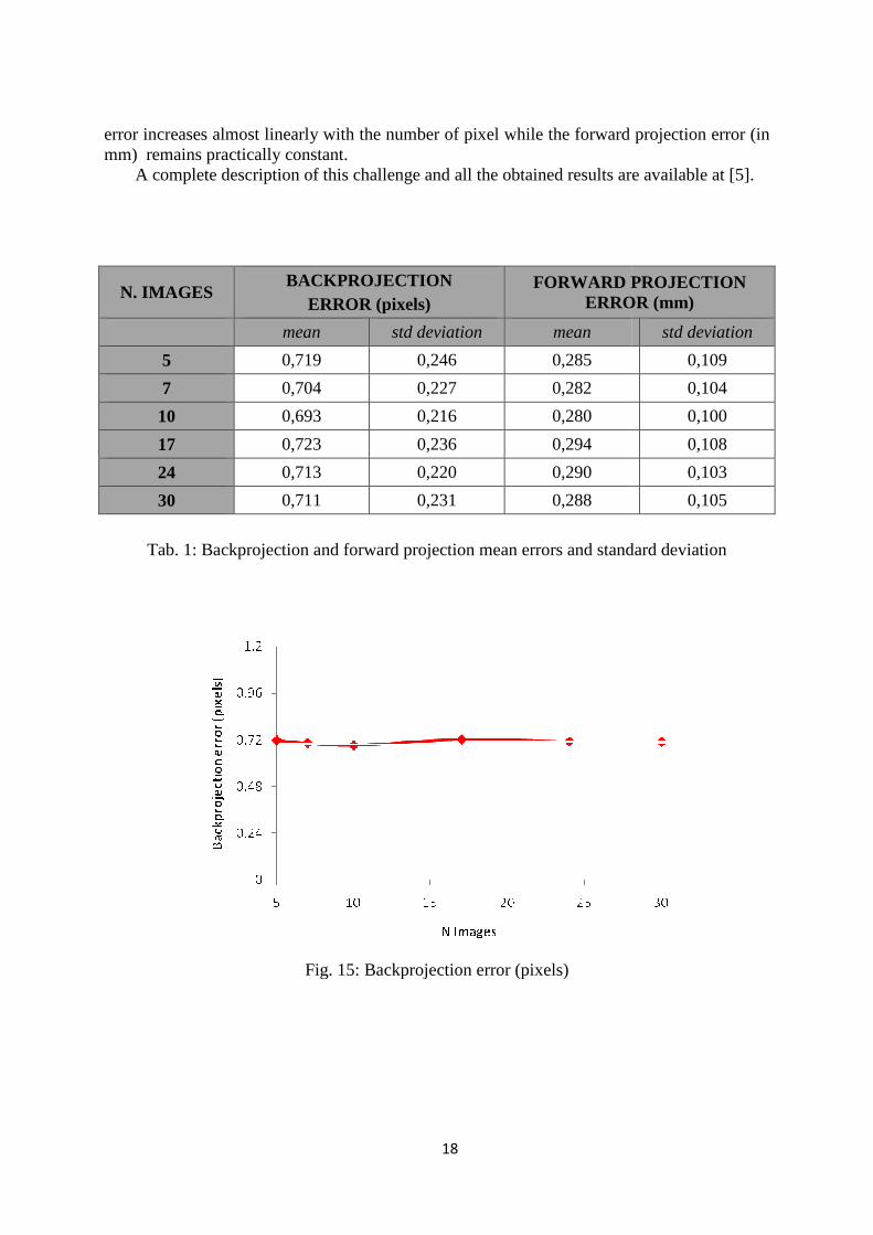
Table 1 reports the results obtained running the OpenCV solution: they indicate how the errors (averaged on all other variable parameters) change when increasing the number of calibration images; these errors are also graphed in Figure 15 and 16.
What we can see is that increasing the number of calibration images, the errors are practically the same. That means that is not so important the number of calibration images but the fact that they cover the whole field of view of the camera in a symmetric way. Another observation we can do is that the forward projection error is, more or less, the same of the measurement uncertainty. This means that the performances of the OpenCV library have reached the limits that can be measured with our test bench.
With respect to the other parameters taken into account, we have observed that a longer optic (with less distortion) provides better results, although it reduces the camera field of view. The same for the quality of the target: HQ results are really more accurate than LQ. Resolution, instead, seems to bring no benefit to the calibration process as the back projection
error increases almost linearly wimm) remains practically constant.
A complete description of this challenge and all the obtained results are available at [5].
N. IMAGES BACKPROJECTION
ERROR (pixels)
mean
5 0,719
7 0,704
10 0,693
17 0,723
24 0,713
30 0,711
Tab. 1: Backprojection and forward
Fig. 15: Backprojection error (pixels)
18
error increases almost linearly with the number of pixel while the forward projection error (in mm) remains practically constant.
A complete description of this challenge and all the obtained results are available at [5].
BACKPROJECTION ERROR (pixels)
FORWARD PROJECTIONERROR (mm)
mean std deviation mean
0,719 0,246 0,285
0,704 0,227 0,282
0,693 0,216 0,280
0,723 0,236 0,294
0,713 0,220 0,290
0,711 0,231 0,288
Tab. 1: Backprojection and forward projection mean errors and standard deviation
Fig. 15: Backprojection error (pixels)
th the number of pixel while the forward projection error (in
A complete description of this challenge and all the obtained results are available at [5].
FORWARD PROJECTION ERROR (mm)
std deviation
0,109
0,104
0,100
0,108
0,103
0,105
projection mean errors and standard deviation
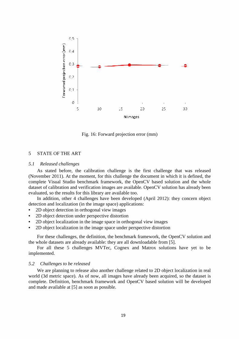
Fig. 16: Forward projection error (mm)
5 STATE OF THE ART
5.1 Released challenges
As stated before, the calibration challenge is the first challenge that (November 2011). At the moment, for this challenge the document in which it is defined, the complete Visual Studio benchmark framework, the OpenCV based solution and the whole dataset of calibration and verification images are available. OpenCV sevaluated, so the results for this library are available too.
In addition, other 4 challenges have been developeddetection and localization (in the image space) • 2D object detection in orthogonal • 2D object detection under • 2D object localization in the image space • 2D object localization in the image space
For these challenges, the definition, the the whole datasets are already available
For all these 5 challenges MVTec, Cognex and Matrox solutions haveimplemented.
5.2 Challenges to be released
We are planning to release also another challenge reworld (3d metric space). As of complete. Definition, benchmark framework and and made available at [5] as soon as possible.
19
Fig. 16: Forward projection error (mm)
As stated before, the calibration challenge is the first challenge that (November 2011). At the moment, for this challenge the document in which it is defined, the complete Visual Studio benchmark framework, the OpenCV based solution and the whole dataset of calibration and verification images are available. OpenCV solution has already been evaluated, so the results for this library are available too.
In addition, other 4 challenges have been developed (April 2012): they concern object (in the image space) applications:
rthogonal view images nder perspective distortion in the image space in orthogonal view images in the image space under perspective distortion
definition, the benchmark framework, the OpenCV solution the whole datasets are already available: they are all downloadable from [5]
For all these 5 challenges MVTec, Cognex and Matrox solutions have
Challenges to be released
to release also another challenge related to 2D object localization in real of now, all images have already been acquired, so the dataset
Definition, benchmark framework and OpenCV based solution willas soon as possible.
As stated before, the calibration challenge is the first challenge that was released (November 2011). At the moment, for this challenge the document in which it is defined, the complete Visual Studio benchmark framework, the OpenCV based solution and the whole
olution has already been
they concern object
enchmark framework, the OpenCV solution and downloadable from [5].
For all these 5 challenges MVTec, Cognex and Matrox solutions have yet to be
2D object localization in real all images have already been acquired, so the dataset is
OpenCV based solution will be developed
20
6 REFERENCES
[1] http://www.progetti.t3lab.it/vialab/ [2] W. Eckstein, Comparing Apples with Oranges - The Need of a Machine Vision Software
Benchmark, INSPECT 12/2009. [3] R. Eastman, et Al., Performance Evaluation and Metrics for Perception in Intelligent
Manufacturing, in Performance Evaluation and Benchmarking of Intelligent Systems, Springer, 2009.
[4] http://en.wikipedia.org/wiki/Ground_truth [5] http://www.progetti.t3lab.it/vialab/il-progetto/benchmark/ [6] http://opencv.willowgarage.com/wiki/ [7] VIALAB, Survey sull’utilizzo dei sistemi di visione nella filiera dell’automazione, 2011. [8] C. Salati, M. Benedetti, I sistemi di visione aiutano l’automazione, Automazione e
Strumentazione, aprile 2012. [9] http://www.verifysoft.de/en_halstead_metrics.html [10] M. H. Halstead, Elements of Software Science, Elsevier North-Holland, Inc., 1977. [11] http://en.wikipedia.org/wiki/Halstead_complexity_measures#cite_note-0 [12] http://en.wikipedia.org/wiki/Receiver_operating_characteristic [13] JCGM 200:2008, International vocabulary of metrology — Basic and general concepts
and associated terms (VIM), 2008. [14] N. Pinto, D.D. Cox, J.J. DiCarlo, Why is Real-World Visual Object Recognition Hard?,
PLoS Computational Biology, 4(1), 2008. [15] http://tev.fbk.eu/DATABASES/objects.html
7 ACKNOLEDGMENTS
We are pleased to acknowledge the contribution that we have received from engineers F. Ziprani and R. Cipriani and from MARPOSS SpA, that allowed us to access their measurement benches and that provided significant help with all metrological aspects of the definition of the machine vision benchmark.