Purdue UniversityPurdue e-Pubs

LARS Technical Reports Laboratory for Applications of Remote Sensing

1-1-1973

Machine Processing for Remotely Acquired DataD. A. Landgrebe

Follow this and additional works at: http://docs.lib.purdue.edu/larstech

This document has been made available through Purdue e-Pubs, a service of the Purdue University Libraries. Please contact epubs@purdue.edu foradditional information.

Landgrebe, D. A., "Machine Processing for Remotely Acquired Data" (1973). LARS Technical Reports. Paper 29.http://docs.lib.purdue.edu/larstech/29

. ,

r ., ,

LARS Information Note 031573

Machine Processing for Remotely Acquired, Data

by D. A. Landgrebe

The Laboratory for Applications of Remote Sensing

Purdue University, West Lafayette, Indiana

1973

A slightlyorevised version of this contribution will be published as a chapted in "Remote Sensing of Environ­ment," edited by Joseph Lintz, Jr. and David S. Simonett, ©1974, Addison-Wesley Publishing Company, Advanced Book Program, Reading, Massachusetts 01867.

LARS Information Note 031573

Machine Processing for Remotely Acquired Data

by

D. A. Landgrebe

PREFACE

This paper presents a general discussion intended to introduce the prospective user to multivariate data analysis techniques as applied to the processing of re­motely acquired earth observational data. Not only are numerically-oriented remote sensing systems discussed, but attention is given to image-oriented systems, the other main branch of remote sensing, in order to estab­lish the relationship between the two.

This Information Note is a major revision of Information Note 041571, w~ich is now obsolete. During the time of preparation, LARS was supported in part by NASA Grant NGL 15-005-112.

-2-

ABSTRACT

This paper is a general discussion of earth resources information systems which utilize airborne and spaceborne sensors. It points out that informa­tion may be derived by sensing and analyzing the spectral, spatial and temporal variations of electro­magnetic fields emanating from the earth surface. After giving an overview system organization, the two broad categories of system types are discussed. These are systems in which high quality imagery is essential and those more numerically oriented. Sensors are also discussed with this categorization of systems in mind.

The multispectral approach and pattern recog­nition are described as an example data analysis procedure for numerically-oriented systems. The steps necessary in using a pattern recognition scheme are described and illustrated with data obtained from aircraft and the Earth Resources Technology Satellite (ERTS-l). Both manual and machine-aided training techniques for the pattern recognition algorithm are described. Other data processing activities are also mentioned.

Section I: INTRODUCTION: WHAT IS REMOTE SENSING? HOW IS INFORMATION CONVEYED?

Imagine that you are high above the surface of the earth looking down. You want to survey the earth's surface in order to learn about its resources and thus to manage them better. How could this in­formation be derived? What might the system to extract it look like?

Remote sensing provides some answers. Remote sensing is the science and art of acqu1r1ng informa­tion about material objects from measurements made at a distance, without physical contact with them. In remote sensing, information may be transmitted to the observer either through force fields or electro­magnetic fields, and in particular, through the

• Spectral, • Spatial, and • Temporal

variations of these fields. Therefore, in order to derive information from these field variations, one must be able to

-3-

• Measure these variations and Relate these measurements to those of known objects or materials 1 •

If, for example, one desires a map showing all of the water bodies of a certain region of the earth, it is clear that one cannot sense the water directly from spacecraft altitudes, rather only the manifestations of these water bodies which exist at that height. These manifestations, in the form of electromagnetic radiation, must therefore be measured and the measure­ments analyzed to determine which points on the earth contain water and which do not.

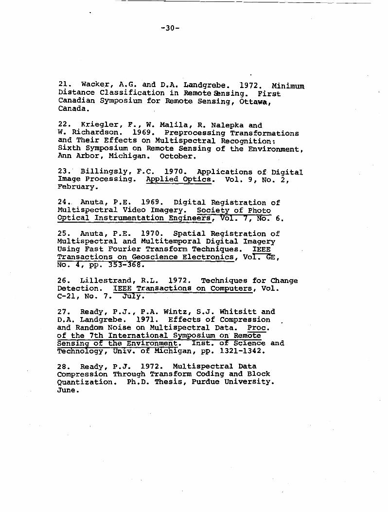
This paper concerns electromagnetic fields, which appear to have a greater potential than force fields. Figure 1 reviews the spectrum of electromagnetic fields. The visible portion, extending from 0.4 to 0.7 micro­meters, is the most familiar to us as it is this portion of the spectrum to which our eyes are sensitive: however, sensors can be built to cover a much broader range of wavelengths. The entire portion frOm 0.3 to 15 micrometers, referred to as the optical wavelength portion, is particularly of interest. The wavelengths shorter than 0.4 micrometers are in the ultraviolet region. The portion above the visible spectrum is the infrared region, with 0.7 to approximately 3 micro­meters referred to as the reflective infrared and the region from 3 to 15 micrometers called the emissive or thermal infrared region. In this latter portion of the spectrum, energy is emitted from the body as a result of its thermal activity or heat rather than reflected from it. .

In addition to the optical wavelengths, pre­liminary results using passive microwave and radar sensors indicate considerable promise for this micro­wave portion of the spectrum. For reasons of sim­plicity and in the interest of time, however, we shall limit our considerations in the remainder of this discussion to the optical portion of the spectrum.

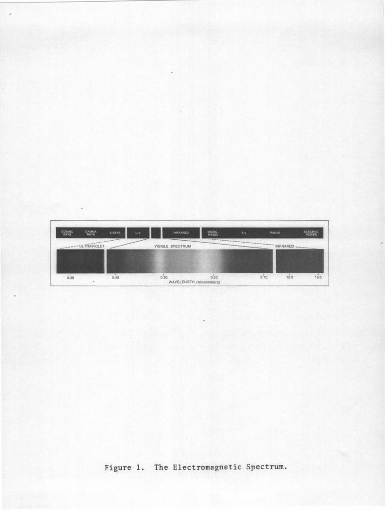
Figure 2 is a diagram of the organization of an earth survey system. It is necessary, of course, to have a sensor system viewing that portion of the earth under consideration. There will necessarily be a certain amount of on-board data processinq. This will perhaps include the merging of data from other sources such as sensor calibration data and data de­lineating where the sensor was pointed.

-4-

One must next transport the data back to earth for further analysis and processing. This may be done through a telemetry system, as in the case 'of the Earth Resources Technology Satellite, or through direct package return, as used with SKYLAB. There usually then is a need for certain preprocessing of the data before the final processing with one or more data reduction algorithms. It is at this point in the system, when the data is reduced to informa­tion, that it is usually helpful to merge ancillary information, perhaps derived from sources on the surface of the. earth.

An important part of the system which must not be overlooked is indicated by the last block in Figure 2, that of information consumption, for there is no reason to go through the whole exercise if the information produced is not to be used. In the case of an earth resource information system, this last portion can prove to be" the most challenging to design and organize since the many potential consumers of this information are not accustomed to receiving it from a space system and may indeed know very little about its information-providing capabilities.

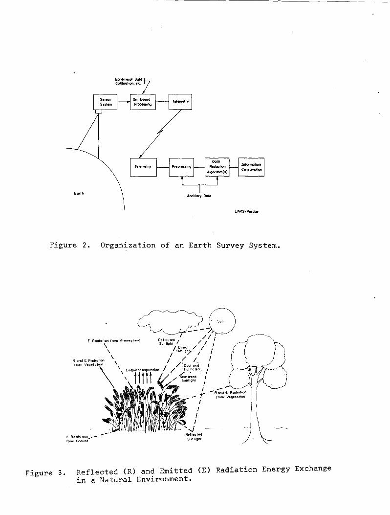
It is necessary to thoroughly understand the portion of the system preceeding the sensor, particularly the energy exchange in a natural environment (Figure 3). It is possible, of course, to detect the presence of vegetation by measuring its reflected and emitted radiation. One must understand, however, that many experimental variables are active. For example, the sun provides a relatively constant source of illumi­nation from above the atmosphere, but the amount of radiation which is reflected from the earth's surface depends upon the condi tioD of the atmosphere, the existence of surrounding objects, and the angle bet-ween the sun and the earth's surface as well as the angle between the earth's surface and the point of observation. Even more important is the variation in the vegetation itself. It is possible to deal with these experimental variables in several ways. These will be discussed later.

Summarizing, then, it is possible to derive information about the earth's surface and the condition of its resources by measuring the spectral, spatial, and temporal variations of the electromagnetic fields emanating from points of interest and then analyzing these measurements to relate them to specific classes of materials. To do so, however, requires an adequate understanding of the materials to be sensed and, in order to make the information useful, a precise know­ledge is required about how the information will be

-5-

used and by whom.

Section II: THE TWO MAJOR BRANCHES OF REMOTE SENSING

When we consider remote sensing today, the field has two major stems originating from two different technologies. These two types of systems will be re­ferred to here as those with

• Image orientation, and • Numerical orientation.

An example of an image-oriented system might be simply an aerial camera and a photo-interpreter. Photographic film is used to measure the spatial variations of the electromagnetic fields, and the photo-interpreter relates these variations to specific classes of surface cover. Numerically oriented sys­tems, on the other hand, tend to involve computers for data analysis. Although the photo-interpreter , and the computer, respectively, tend to be the identify­ing components in each type of system, it is an over­simplification to say that they are uniquely related to them. This becomes clearer upon further examination.

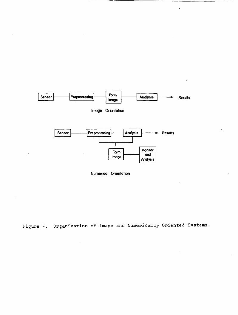
Comparing the two systems (Figure 4), both types need a sensor and some preprocessing: however, the distinction between the types can perhaps be brought out most clearly by noting the location of the "form image" block in the two diagrams. In the image-orient­ed type, it is a step in the data stream and must pre­cede the analysis. Numerically oriented systems, on the other hand, need not necessarily form an image. If they do, and in earth resources work they usually do, it may be at the side of the ~ata stream, as shown. Images may be used to monitor the system and perhaps to do some special analysis. An image is, of course, the most efficient way to convey a large amount of information to a human operator. Thus, both types of systems, use images but the use is different in the two cases.

Section III: SENSOR TYPES AS RELATED TO SYSTEM TYPES

In considering the design of information gather­ing systems, it is important that the type of sensor as well as the means of analysis are well-mated to the type of system orientation. Thus, let us brief­ly consider the types of imaging spaceborne sensors available.

-6-

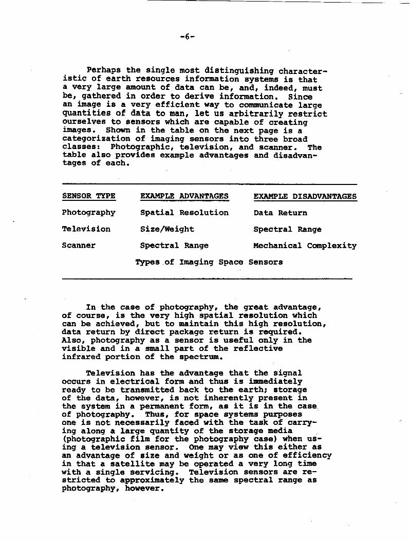
Perhaps the single most distinguishing character­istic of earth resources information systems is that a very large amount of data can be, and, indeed, must be, gathered in order to derive information. Since an image is a very efficient way to communicate large quantities of data to man, let us arbitrarily restrict ourselves to sensors which are capable of creating images. Shown in the table on the next page is a categorization of imaging sensors into three broad classes: Photographic, television, and scanner. The table also provides example advantages and disadvan­tages of each.

SENSOR TYPE

Photography

Television

Scanner

EXAMPLE ADVANTAGES

Spatial Resolution

Size/Weight

Spectral Range

EXAMPLE DISADVANTAGES

Data Return

Spectral Range

Mechanical Complexity

Types of Imaging Space Sensors

In the case of photography, the great advantage, of course, is the very high spatial resolution which can be achieved, but to maintain this high resolution, data return by direct package return is required. Also, photography as a sensor is useful only in the visible and in a small part of the reflective infrared portion of the spectrum.

Television has the advantage that the signal occurs in electrical form and thus is immediately ready to be transmitted back to the earth, storage of the data, however, is not inherently present in the system in a permanent form, as it is in the case of photography. Thus, for space systems purposes one is not necessarily faced with the task of carry­ing along a large quantity of the storage media (photographic film for the photography case) when us­ing a television sensor. One may view this either as an advantage of size and weight or as one of efficiency in that a satellite may be operated a very long time with a single servicing. Television sensors are re­stricted to approximately the same spectral range as photography, however.

-7-

Scanners can be built to operate over the entire optical wavelength range. They can also provide a greater photometric dynamic range. In order to achieve these advantages, however, they tend to be more mechani­cally cOmplex.

It is tmportant to realize that the advantages and disadvantages here must be considered only as examples since the advantages and disadvantages in any specific instance will depend upon the precise details of the system. General statements are also difficult relative to the type of sensors which will be best for image-oriented and numerically oriented systems. There is a clear tendency to favor photo­graphy for image-oriented systems due to its high spatial resolution capability, while multiband scanners tend to be favored for numerically oriented systems since they make available greater spectral and dynamic ranges.

The technology for pictorially oriented systems is relatively well-developed. Sensors best suited to this type of system have long been in use, as have appropriate analysis techniques. This type

.of system also has the advantage of being easily acceptable to the layman or neophyte, an advantage important in the earth resources field, with its many new data users. Similarly, it is well-suited for producing subjective information and is especially suited to circumstances where the classes to be ident­ified in analysis cannot be precisely selected befor~­hand. Thus, man with his superior intelligence is or can be, deeply involved in the analysis activity. Pictorially oriented systems also have the possibility of being relatively simple and low-cost. On the other hand, it is difficult to use them for large-scale sur­veys over very large areas involving very large amounts of data.

In the case of numerically oriented systems, the technology is much newer and not nearly so well-developed, though very rapid progress is being made. Secause the various steps involved tend to be more abstract, they tend to be less readily understandable to the layman. This type of system is best suited for producing ob­jective information, and surveys covering large areas are certainly possible. Numerically oriented systems tend to be generally more complex, however.

In summary, the state of-the-art is that there are two general branches of remote sensing1 this duality exists primarily for historical reasons and because these technologies began at different points.

-8-

One type is based on imagery, and, therefore, a key goal of an intermediate portion of the system is the generation of high-quality imagery. In the other case imagery is less important and indeed may not be necessary at all. It is not appropriate to view these two types of systems as being in competition with one another since they have different capabilities and are useful in different circumstances.

Numerically oriented systems and a particular type of data analysis useful for them will now be examined. .

Section IV: THE MULTISPECTRAL APPROACH AND PAT'l'ERN RECOGNITION

How does one begin the task of devising a tech­nique for analyzing large quantities of remotely sensed earth observational data? Certainly one must make optimum use not only of man's ability but also of modern computer devices. This consideration strongly influenced the route that the technology has taken. Though much basic research effort has been expended, few practical methods have been un­earthed for the machine analysis of data as complex as earth observational imagery based upon the spatial variations in the scene. Thus, if much of the routine and repetitive aspects of the analysis are to be successfully turned over to a machine. so that low-cost, high-throughput analysiS is obtained, a fundamentally simpler approach must be taken. Basing the analysis primarily on temporal variations in the scene held reason for concern in early work also, since, in this case, no information could be derived based solely on observations taken at a single point in time.

Fortunately, the third of the three, Spectral variations, did appear to hold promise for machine analysis based upon feasibility studies into what has come to be called the multispectral approach. The route taken by the numericai-Sranch of remote sensing has been to utilize spectral variations as fundamental to the analysis later adding to the processing the use of spatial and temporal information as circumstances require and permit.

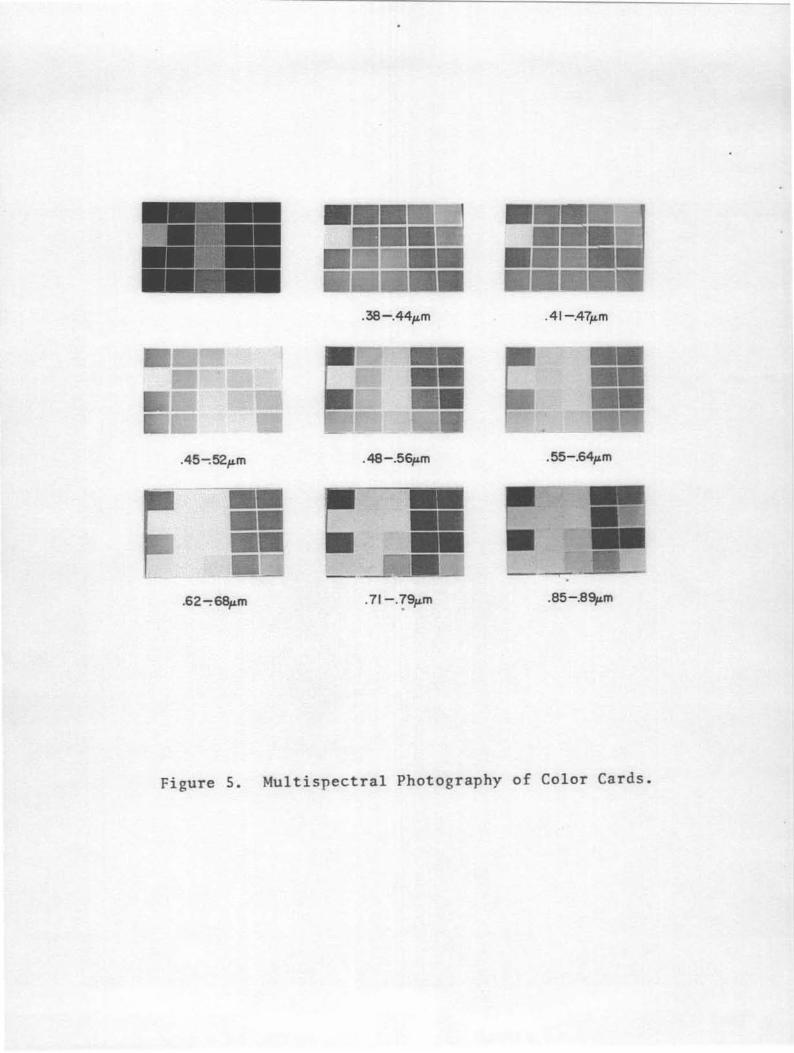
An initial understanding of what is meant by the term "multispectral approach" may be obtained by con­sidering Figure s. Shown here in the upper left of the figure is a reproduction of a conventional color

-9-

photograph of a set of color cards. The remainder of the figure shows photographs of the same color cards taken with black and white film and several dif~erent filters. The pass band of each filter is indicated beneath the particular color and card set. For example, in the .62-.66 micrometer band, which is in the red portion of the visible spectrum, the red cards appear white in the black and white photo, indi­cating a high response or a large amount of red light energy being reflected. In essence the multispectral approach amounts to identifying any color by noting the set of gray scale values produced on the black and white photographs for that particular color rectangle.

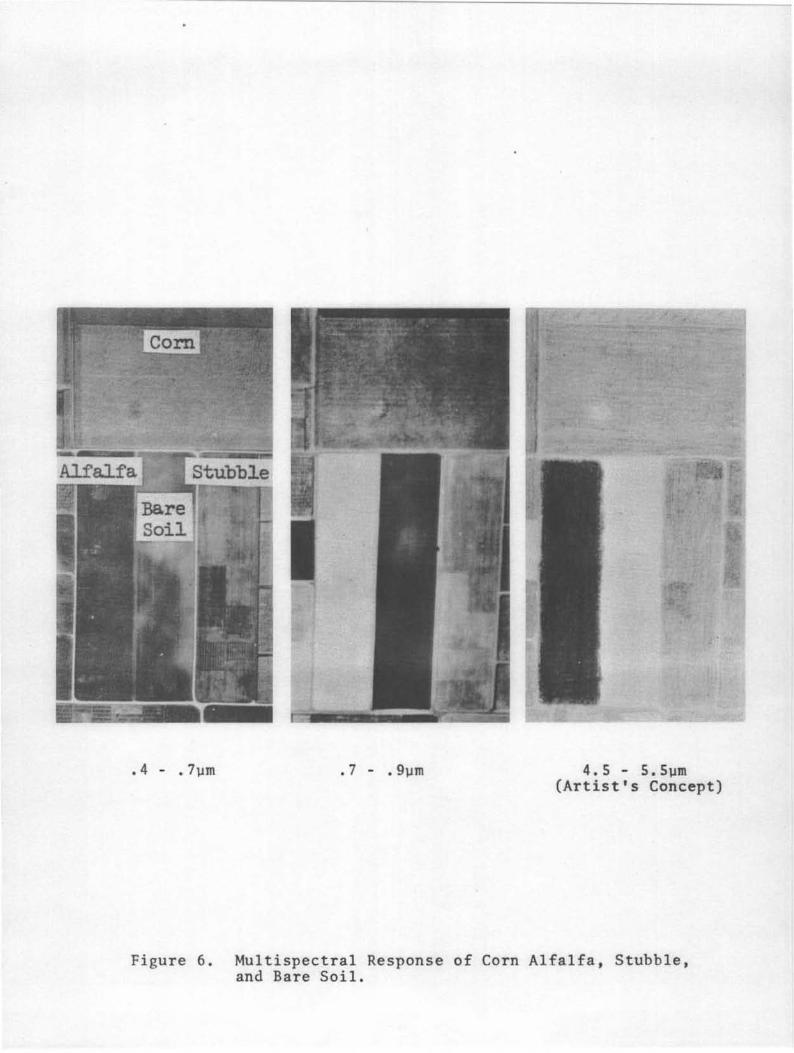
As a very simple example of the approach Figure 6 shows images of an agricultural scene taken in three different portions of the spectrum2• Note that in the three bands alfalfa has responses which are dark, light, and dark, respectively, whereas bare soil is gray, dark and white. Thus, alfalfa cap be discriminated from bare soil by identifying the fields which are dark, light, dark in order in these three spectral bands.

One may initially think of the multispectral approach as one in which a very quantitative measure of the color of a material is used to identify it. Color, however, is a term usually limited to the re­sponse of the human eye1 the precise terminology of spectroscopy is more useful in understanding the multispectral approach, and isoapplicable beyond the visible regio!]..

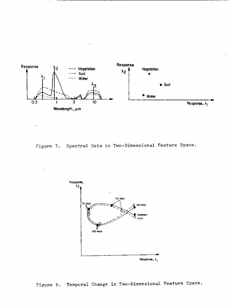
In order to understand this approach and to see how a numerically oriented system may be based upon it, consider Figure 7. Shown at the left is a graph of relative response (reflectance) as a function of wavelength for three types of earth-surface cover material: vegetation, soil and water. Let two wave­lengths marked ~i and A2 be selected. Shown in the lower part of this figure is the data for these three materials at these two wavelengths, plotted with re­spect to one another. For example, in the left soil has the largest response at wavelength A11 this mani­fests itself in the right plot in the fact that soil has the largest abscissa value (the greatest displace­ment to the right).

It is readily apparent that two materials whose response as a function of wavelength are different will lie in different portions of the two-dimensional space.. When this occurs one speaks of the materials

*This space is referred to as feature space.

-10-

involved as having unique spectral signatures. This concept will be pursued further. presently: however, at this point it is important to recognize that the concept of a spectral signature is a relative one--one cannot know that vegetation has a unique spectral signature, for example, until he sees the plots resulting from the spectral response of other materials within the scene to be analyzed.

Note a180 that a larger number of bands can be used. The response at ~J could be used and the data plotted in three dimensions. Pour or more dimensions indeed have meaninq and utility even though an actual plot of the data is not possible.

So far no temporal nor spatial information has been involved, only spectral. Temporal information can be utilized in several ways. Time is always a para­meter of the spectral response of surface materials. As an example, consider the problem of discriminatinq between soybeans and corn, and refer to Fiqure 8. Under cultivation, these two plants have approximately 140-day growing cycles. Piqure 8 illustrates what the two-dimensional response plot might be for fields of these two species with time as a parameter". Upon planting and for some period thereafter, fields of soy­beans and corn would merely appear to be bare soil from an observation platform above them. Event­ually though, both plants would emerge from the soil and in time develop a canopy of green veqetation, mature to a brownish dry vegetation, and diminish. Thus, as viewed from above, the fields of soybeans and corn would in fact, always be mixtures of green vege­tation and soil. In addition to the vegetation of the two plants having a slightly different response as a function of wavelength, the growing cycles and plant geometries are differentJ thus, the mixture parameters miqht (and in fact do) permit an even more obvious difference between the two plants than the spectral response difference of the plant leaves them­selves. This is the implication in Pigure 8 as shown by the rather large difference between them 30 days from planting date (partial canopy) as compared to 75 days (full canopy). Thus, one way in which temporal information is used is simply in determining the optimum time at which to conduct a survey of given materials.

A second use of temporal information is perhaps less obvious. Consider the situation of Figure 8 at the 75-day and 100-day points. In this case the separ­ation of the two materials is relatively slight.

-11-

However, if this data is replotted in four-dimensional space, response at Al and A2 and 75 days as dimensions one and two and Al and A2 at 100 days as dimensions three and four, the small separabilities at the two times can often be made to augment one another.

A third use of temporal information is simply that of change detection. In many earth resources problems it is necessary to have an accurate histori­cal record of the changes taking place in a scene as a function of time.

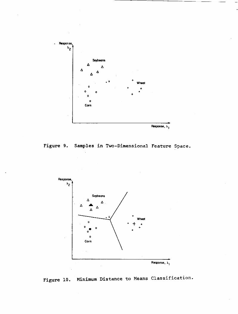
Let us consider how one may devise a procedure for analyzing multispectral data. s ,- In the process, one further facet of the multispectral approach must be taken into account. The radiation from all soy­beans fields will not have precisely the same spectral response, since all will not have had the same planting date, soil preparation, moisture conditions and so on. Moreover, response variation within a class may be expected of any earth-surface cover. The extent of response differences of this type cer­tainly has an effect upon the existence of a spectral signature, that is, the degree of separability of one material from another. Consider, for example, a scene composed of soybeans, corn and wheat fields: if five samples of each material are drawn, the two­dimensional response patterns might be as shown in Figure 9 indicating some variability exists within the three classes. Suppose now an unknown point is drawn from the scene and plotted, as indicated by the point marked U.

The design of an analysis system in this case comes down to partitioning this two-dimensional feature space in some fashion, such that each such possible unknown point is uniquely associated with one of the classes. The engineering and statistical literature abounds with algorithms or procedures by which this can be done. s " In order to illustrate the concept, one very simple one is shown in Figure 10. In this case the conditional centroid or center point of each class is first determined. Next the locus of points equidistant from these three centroids is plotted and results in the three segments of straight lines as shown·. These lines form, in effect, decision boundaries. In this example the unknown point "U" would be associated with the class soybeans as a result of the location of it with respect to the decision boundaries.

*When more than two dimensions (spectral bands) are being used, note that this locus would become a sur­face rather than a line.

-12-

In very simple situations where data from the various classes are quite well separated in this feature space, an even simpler technique, called "level-slicing-, can be used. The term level-slicing came into use when analysts of black and white photo­graphy began identifying (Figure 6) certain materials from others in a scene by their range of gray levels. Thus, by identifying the areas on the film which had this range or slice of levels, one could locate all of the regions containing that material.

This simple concept immediately extends to the multiband case where one looks for areas in which the data falls in one range in the first band, a second range in band two, and so on. From the feature space viewpoint this method identifies data points which fall in a horizontally or vertically oriented rectangle.

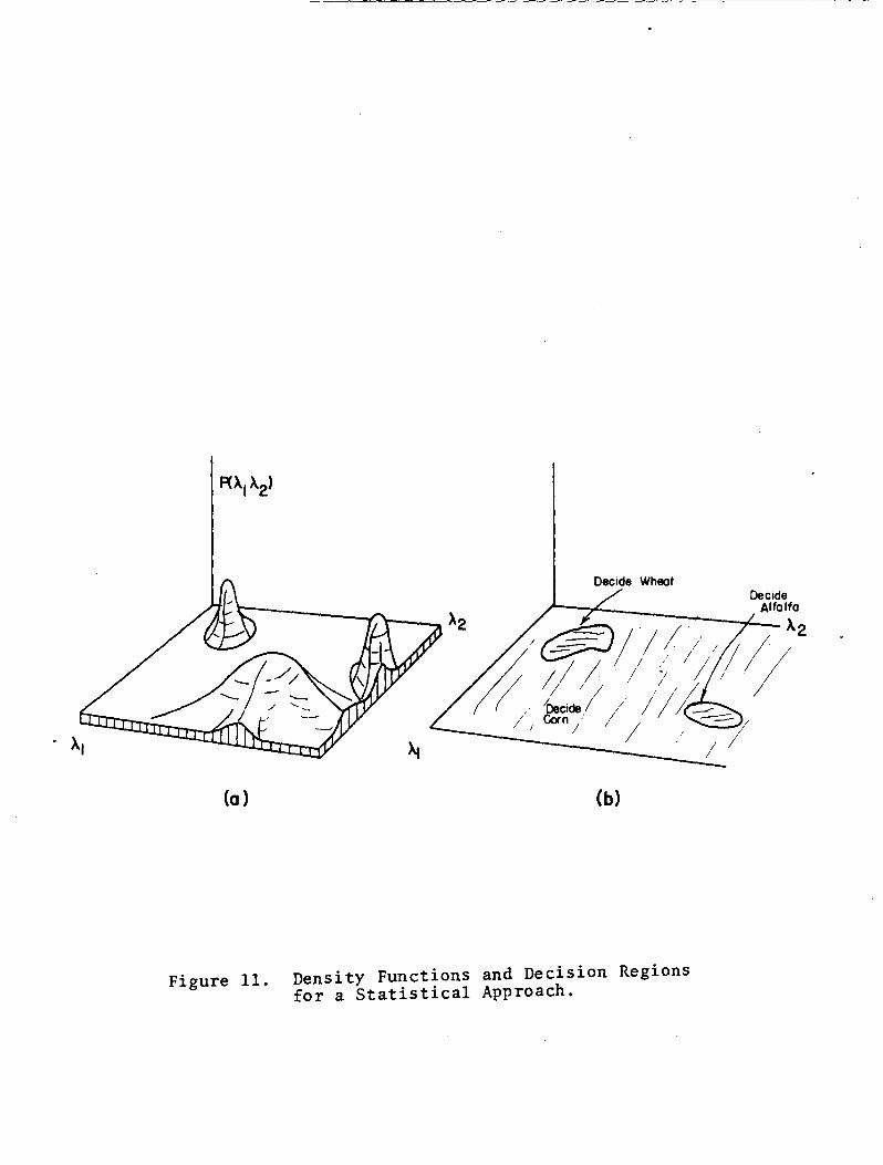
For many analysis problems of practical interest, a somewhat more sophisticated procedure allowing for more generality in the location and form of the decision boundaries is called for. One such algorithm, the so called Gaussian Maximum Likelihood Classifier, has been especially well-studied for this purpose. In this case" the initial samples of each class are used to estimate not only the mean value for each class, but also its covariance matrix. This latter matrix shows not only the variange present in data from each spectral band but also the degree of correlation between bands. Under the assumption that the data from each class have a Gaussian (or bell-shaped) distribution, these mean values and covariance matrix completely define the class distribution and for the two spectral band ~ase they might appear as shown in Figure 11 (a). A given data point is then assigned to a class accord-ing to which class Gaussian density function has the largest value (or maximum likelihood) for that response value in Al & A2. Thus, the decision boundaries occur at the intersection of class density function as shown in Figure 11 (b) and, are in general segments of second order curves, i.e. parabolas, hyperbolas, ellipses, and circles with straight lines as a de­generate case.

This technique of analysis is referred to as pattern recognition, and there are many even more sophisticated p~ocedures resulting in both linear and nonlinear decision boundaries. However, the procedure of using a few initial samples to determine the deci­sion boundaries is common to a large number of them. The initial samples are referred to as training sam­ples, and the general class of classifiers in which training samples are used in this way are referred

-13-

to as supervised classifiers.

Section V: THE.MULTISPECTRAL SCANNER AS A DATA SOURCE

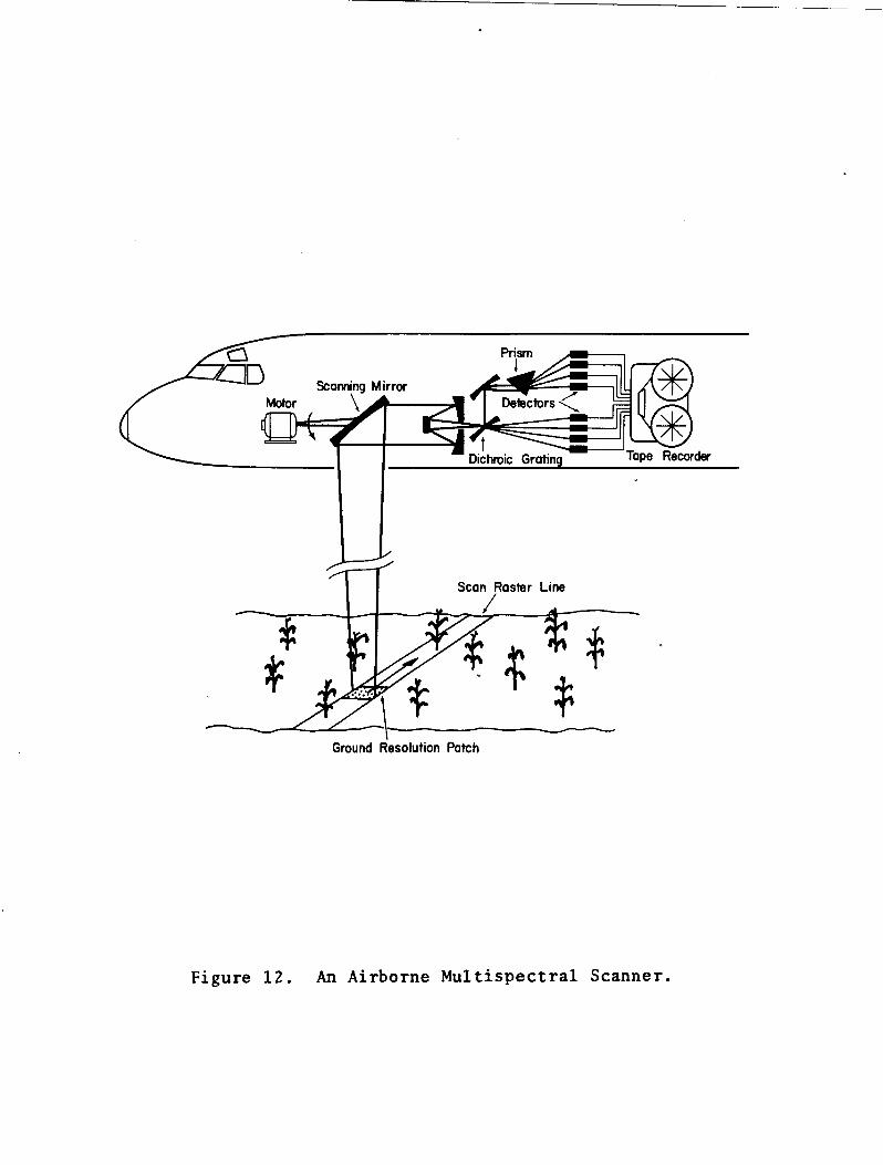
Up to this point, the implication has been that photography or multispectral photography is the sensor to be used in generating data for this type of an analysis procedure. While indeed this data source can be used, a perhaps more appropriate one is as a multi­spectral scanner. Figure 12 diagrams such a device as might be mounted in an aircraft.

Basically the device consists of a multiband spectrometer whose instantaneous field of view is scanned across the scene. The scanning in this case is accomplished by a motor-driven scanning mirror. At a given instant the device is gathering enerqy from a single resolution element. The energy from this element passes through appropriate optics and may, in the case of the visible portion of the speetrum, be directed through a prism. The prism spreads out the energy according to the portion of the spectrum; detectors are located at the output of the prism. The output of the detectors can then be recorded on magnetic tape or transmitted directly to the ground. Gratings are commonly used as dispersive devices for the infrared portion of the spectrum.

A most important property of this type of system is that all enerqy fram a given scene element in all parts of a spectrum pass through the same optical aperture. 'rhus, by simultaneously sampling the output of all detectors one has, in effect, deter­mined the response as a function of wave-lenqth for the scene element in view at that instant.

Of course, the scanninq mirror causes the scene to be scanned across the field of view transverse to the direction of platform motion, and the motion of the platform (aircraft) provides the appropriate motion in the other dimension so that in time every element in the scene has been in the instantaneous field of view of the instrument.

Section VI: AN ILLUSTRATIVE EXAMPLE

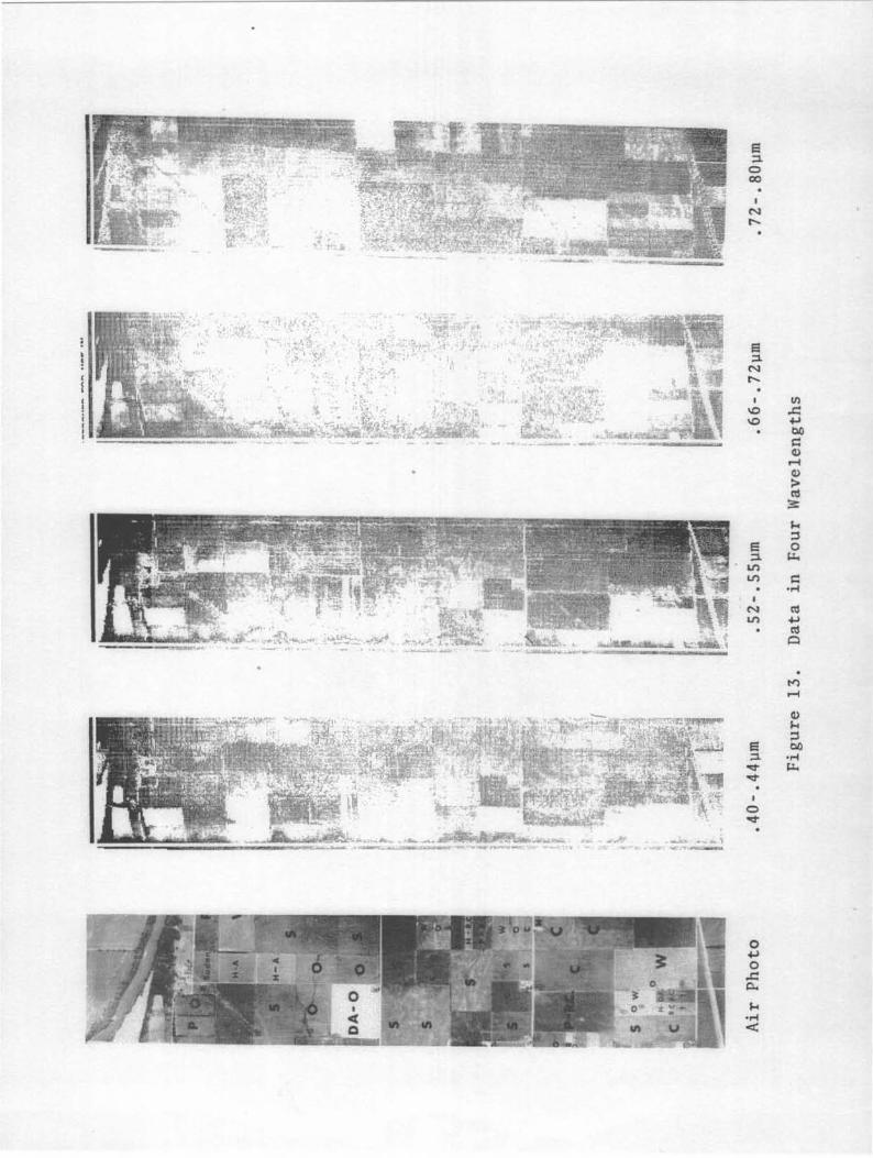
As an example of the use of this type of sensor and analysis procedure, results of the analysis of a flightline will be presented in brief form*. The particular example involves the classification of a one-mile bv four-mile area into classes of

*This example was originally prepared by Professor Roger Hoffer of LARS/Purdue.

-14-

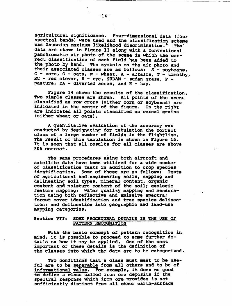
agricultural significance. Four-dimensional data (four spectral bands) were used and the classification scheme was Gaussian maximum likelihood discrimination.' The" data are shown in Figure 13 along with a conventional panchromatic air photo of the scene in which the cor­rect classification of each field has been added to the photo by hand. The symbols on the air photo and their associated classes are as follows: S - soybeans, C - corn, 0 - oats, W - wheat, A - alfalfa, T - timothy, RC - red clover, R - rye, SUDAN - sudan grass, P -pasture, DA - diverted acres, and H - hay.

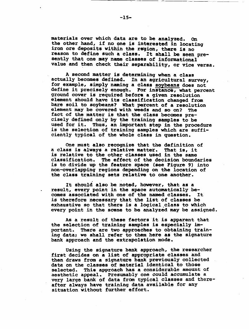
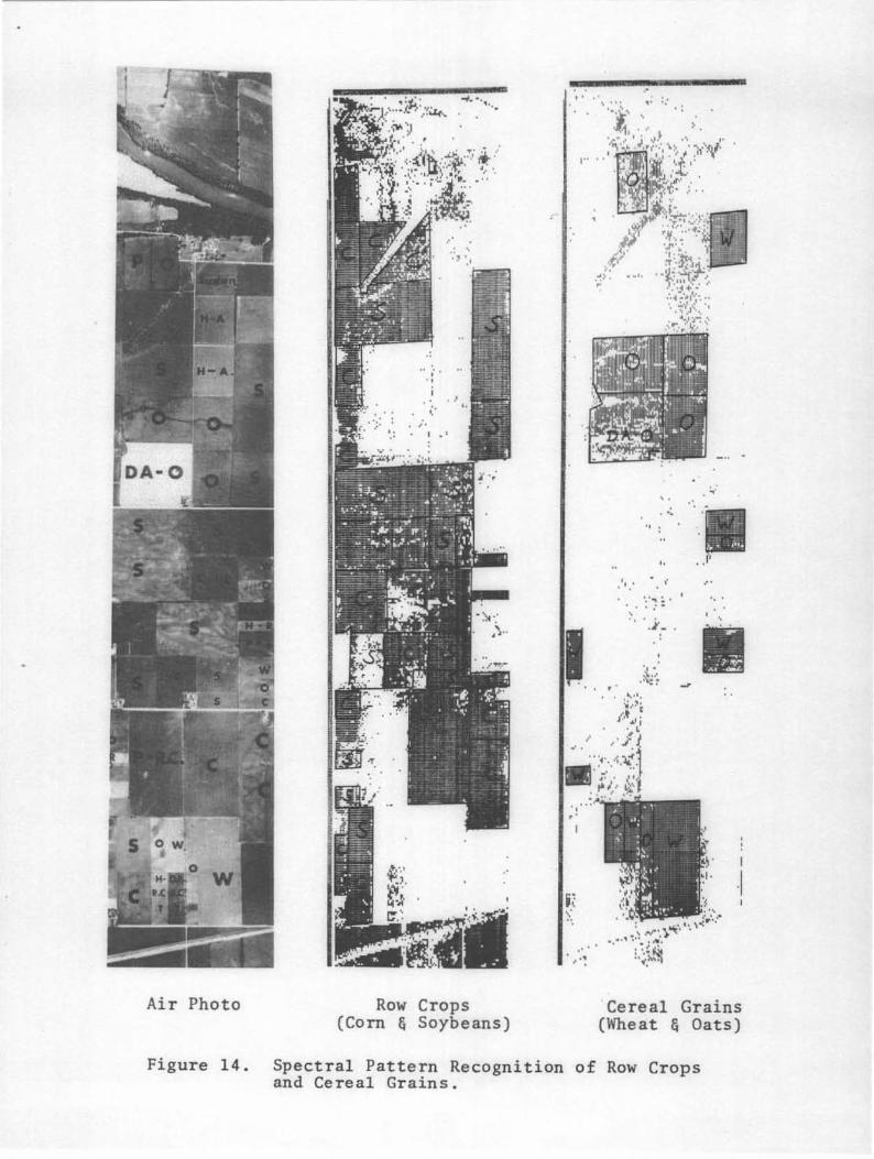
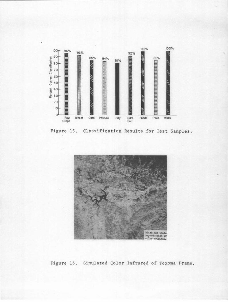
Figure 14 shows the results of the classification. Two simple classes are shown. All points of the scene classified as row crops (either corn or soybeans) are indicated in the center of the figure. On the right are indicated all points classified as cereal grains (either wheat or oats).

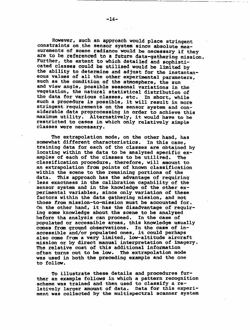
A quantitative evaluation of ~he accuracy was conducted by designating for tabulation the correct class of a large number of field. in the flightline. The result of this tabulation is shown in Figure 15. It is seen that all results for all classes are above 80\ correct.

The same procedures using both aircraft and satellite data have been utilized for a wide number of classification tasks .in addition to crop species identification. Some of these are as follows: Tests of agricultural and.engineering soils, mapping and delineatinq soil types, mineral content, organic content and moisture content of the soil, geologic feature mapping, water quality mapping and mensura­tion using both reflective and emissive spectral forest cover identification and tree species delinea­tionl and delineation into geographic and land-use mapping categories.

Section VII: SOME PROCEDURAL DETAILS IN THE USE OF PATTERN RECOGNITION

With the basic concept of pattern recognition in mind, it is possible to proceed to some further de­tails on how it may be applied. One of the most important of these details is the definition of the classes into which the data are to be categorized.

Two conditions that a class must meet to be use­ful are to be seiarable from all others and to be of informational va ue. For example, it does no good to define a class called iron ore deposits if the spectral response which iron ore provides is not sufficiently distinct from all other earth-surface

-15-

materials over which data are to be analyzed. On the other hand, if no one is interested in locating iron ore deposits within the re~ion, there is no reason to define such a class. It shall be seen pre­sently that one may name classes of informational value and then check their separability, or vice versa.

A second matter is determining when a class actually becomes defined. In an agricultural survey, for example, simply naming a class soybeans does not define it precisely enough. Por instance, what percent ground cover is required before a given resolution element should have its classification changed from bare soil to soybeans? What percent of a resolution element may be covered with weeds and so on? The fact of the matter is that the class becomes pre­cisely defined only by the training samples to be used for it. Thus, an important step in the procedure is the selection of training samples which are suffi­ciently typical of the whole class in question.

One must also recognize that .the definition of a class is always a relative matter. That is, it is relative to the other classes used in the same classification. The effect of the decision boundaries is to divide up the feature space (see Figure 9) into non-overlappinq regions depending on the location of the class traininq sets relative to one another.

It should also be noted, however, that as a result, every point in the space automatically be-comes associated with one of the named classes. It is therefore necessary that the list of classes be exhaustive so that there is a loqicaloclass to which every point in the scene to be analyzed may be assiqned.

As a result of these factors it is apparent that the selection of training samples is especially im­portant. There are two approaches to obtaining train­ing dataJ we shall refer to them here as the signature bank approach and the extrapolation mode.

Using the signature bank approach, the researcher first decides on a list of appropriate classes and then draws from a siqnature bank previously collected data on the classes of material identical to those selected. This approach has a considerable amount of aesthetic appeal. Presumably one could accumulate a very large bank of data from typical classes and there­after always have training data available for any situation without further effort.

-----------------------~-~--

-16-

However, such an approach would place stringent constraints on.the sensor system since absolute mea­surements of scene radiance would be necessary if they are to be referenced to a future data-gathering mission. Further, the extent to which detailed and sophisti­cated classes could be utilized would be limited by the ability to determine and adjust for the instantan­eous values of all the other experimental parameters, such as the condition of the atmosphere, the sun and view angle, possible seasonal variations in the vegetation, the natural statistical distribution of the data for various classes, etc. In short, while such a procedure is possible, it will result in more stringent requirements on the sensor system and con­siderable data preprocessing in order to achieve this maximum utility. Alternatively, it would have to be restricted to cases in which only relatively s.imple classes were necessary.

The extrapolation mode, on the other hand, has somewhat different characteristics. In this case, training data for each of the classes are obtained by locating within the data to be analyzed specific ex­amples of each of the classes to be utili~ed. The classification procedure, ·therefore, will amount to an extrapolation from points of known classification within the scene to the remaining portions of the data. This approach has the advantage of requiring less exactness in the calibration capability of the sensor system and in the knowledge of the other ex­perimental variables, since only variation of these factors within the data gathering mission, and not those from mission-to-mission must be accounted for. On the other hand, it·has the disadvantage of requir­ing some knowledge about the scene to be analyzed before tha analysis can proceed. In the case of populated or accessible areas, this knowledge usually comes from ground observations. In the case of in­accessible and/or populated ones, it could perhaps also come from a very limited, low-altitude aircraft mission or by direct manual interpretation of imagery. The relative cost of this additional information often turns out to be low. The extrapolation mode was used in both the preceding example and the one to follow.

To illustrate these details and procedures fur­ther an example follows in which a pattern recognition scheme was trained and then used to classify a re­latively larger amount of data. Data for this experi­ment was collected by the multispectral scanner system

-17-

(KSS) of the Earth Resources Technology Satellite, ERTS-l. From its orbital altitude of approximately 9000 kilo­meters (560 miles) this sensor has an instantaneous field of view of approximately 80 meters on the ground. The all-digital system transmits data to the ground in frames of imagery covering a square area 185 kilometers (100 nautical miles) on a side. The data presented in image form would result in an image made up of 2300 scanlines with 3350 samples per scanline. The sensor provides spatially registered data in four spectral bands from .5 to 1.5 micrometers. Thus, a single data set (frame) consists of approximately 7.5 million four­dimensional points.

Though by .the previous illustration it is apparent that pattern recognition techniques can be used effect­ively on data gathered from an airborne system, they are even more ideally suited to satellite-gathered data where it is possible to gather a very large amount of data in a very short time, thus holding significant and important experimental variables constant during the data gathering activity. Said another way, given that a specific problem requires the gathering of a large amount of data, pattern recognition techniques which function efficiently and cost-effectively only on very large quantities of data are ideally suited for the analysis test from the standpoint of data throughput. .

The particular frame of data used for this example is the first frame gathered by the ERTS-l satellite KSS system after its launch (Frame ID 1002-16312). It was gathered on July 25, 1972 and is of the Red "River Valley areas of Texas and Oklahoma. The frame is centered oh a point 15 miles southeast of Durant, Oklahoma and approximately five miles north of the Red River. A simulated color infrared photograph made from the frame is shawn in Figure 16.

A maximum likelihood Gaussian classification scheme was trained using seventeen classes from this data set. The data were then classified into these seventeen spectral classes. Figure 17 shows a dis­play of the classification results in image form. The detailed analysis results themselves, that is, the identifying class number associated with each point plus the likelihood value for it, are stored on mag­netic tape. Figure 17 presents these quantitative results in a form suitable for qualitative evaluation. This figure was constructed by associating each class or group of classes with an individual color. It is noted in passing that as such, then, Figure 17 cannot accurately be called an enhanced image. More

-18-

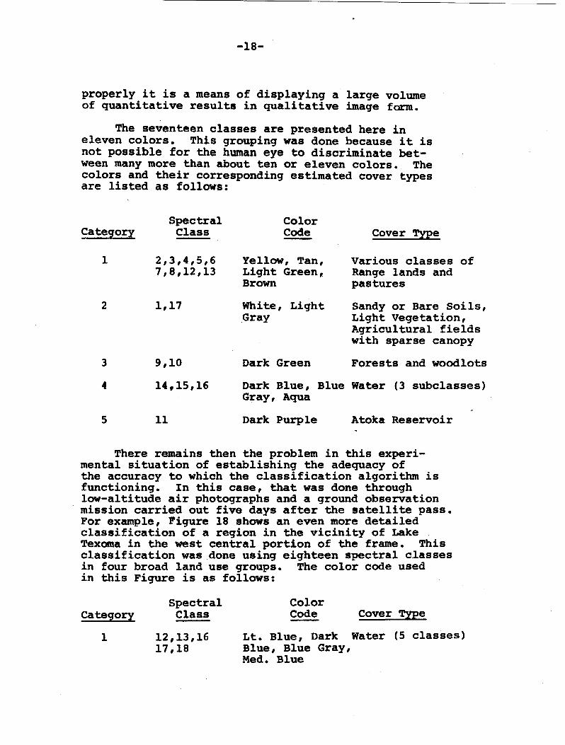
properly it is a means of displaying a large volume of quantitative results in qualitative image farm.

The seventeen classes are presented here in eleven colors. This grouping was done because it is not possible for the human eye to discriminate bet­ween many more than about ten or eleven colors. The colors and their corresponding estimated cover types are listed as follows:

Spectral Color Category Class Code Cover Type

1 2,3,4,5,6 Yellow, Tan, Various classes 7,8,12,13 Light Green, Range lands and

Brown pastures

of

2 1,17 White, Light Sandy or Bare Soils, Gray Light Vegetation,

Agricultural fields with sparse canopy

3 9,10 Dark Green Forests and woodlots

4 14,15,16 Dark Blue, Blue Water (3 subclasses) Gray, Aqua

5 11 Dark Purple Atoka Reservoir

There remains then the problem in this experi­mental situation of establishing the adequacy of the accuracy to which the classification algorithm is functioning. In this case, that was done through low-altitude air photographs and a ground observation mission carried out five days after the satellite pass. For example, Figure 18 shows an even more detailed classification of a region in the vicinity of Lake Texoma in the west central portion of the frame. This classification was done using eighteen spectral classes in four broad land use groups. The color code used in this Figure is as follows:

Category

1

Spectral Class

12,13,16 17,18

Color Code

Lt. Blue, Dark Blue, Blue Gray, Med. Blue

Cover Type

water (5 classes)

-19-

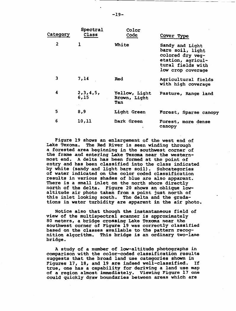
Spectral Color Category Class Code Cover Type

2 1 White Sandy and Light bare soil, light colored dry veg-etation, agricul-tural fields with low crop coverage

3 7,14 Red Agricultural fields with high coverage

4 2,3,4,5, Yellow, Light Pasture, Range land 6,15 Brown, Light

Tan

5 8,9 Light Green Forest, Sparse canopy

6 10,11 Dark Green Forest, more dense canopy

Figure 19 shows an enlargement of the west end of Lake Texoma. The Red River is seen winding through a forested area beginning in the southwest corner of the frame and entering Lake Texoma near the western­most end. A delta has been formed at the point of entry and has been classified into the class indicated by white (sandy and light bare soil). Subcategories of water indicated on the color coded classification results in various $hades of blue are also apparent. There is a small inlet on the north shore directly north of the delta. Figure 20 shows an oblique low­altitude air photo taken from a point just north of this inlet looking south. The delta and the grada­tions in water turbidity are apparent in the air photo.

Notice also that though the instantaneous field of view of the multispectral scanner is approximately 80 meters, a bridge crossing Lake Texoma near the southwest corner of Figure 19 was correctly classified based on the classes available to the pattern recog­nition algorithm. This bridge is an ordinary two-lane bridge.

A study of a number of low-altitude photographs in comparison with the color-coded classification results suggests that the broad land use categories shown in Figures 17, 18, and 19 are indeed well-classified. If true, one has a capability for deriving a land use map of a region almost immediately. Viewing Figure 17 one could quickly draw boundaries between areas which are

-20-

used for various types of agricultural land, range land, forest and other land uses. In addition, the intrinsically quantitative nature of 'the approach allows one immediately to estimate acreages in each land use by counting sample points classed into each of the classes.

A more complete discussion of the analysis of this frame is available in the literature.' Other demonstrations of the use of satellite imagery"10 already have established the accuracy possible with machine analysis for land use mapping purposeS1 future work will no doubt corroborate this conclusion. We will concentrate here therefore on the procedures and computational algorithms necessary to achieve these results.

At present the use of various classification algorithms for this purpose is fairly well understood1 however, the training of an algorithm is still a time-consuming process requiring a trained and sophis­ticated analyst. Earlier it was pointed out that the chosen classes must satisfy two criteria to be valid. They must be separable, a restriction imposed by the reflectance properties of the scene, and they must be of informational value, a restriction imposed by the intended use of the analysis results. Both of these criteria must be simultaneously satisfied.

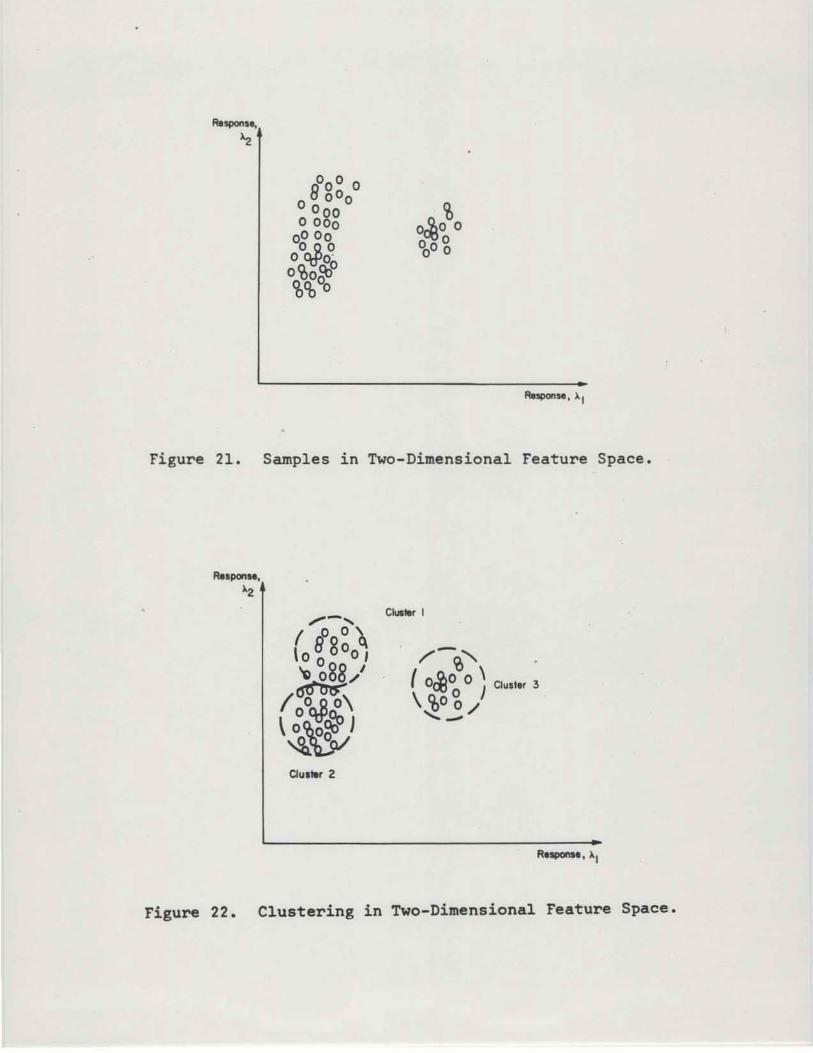
Furthermore, as was previously pointed out, the classes are not really defined until the training data or statistics describing them exist. The diffi­culty of determining eighteen sets of four-dimensional mean vectors and co-variance matrices can ba readily envisioned, particularly if it were necessary to identify the sample points used to estimate these statistics manually. OVer the last few years research has been directed toward machine-aided methods for this process. One such procedure involves the use of a type of classifier not utilizing training samples. It is referred to as an unsupervised classifier. Assume, for example, that one has same two-dimensional data (as shown in Figure 21)1 assume also that one knows there are three classes of material in this data but the correct association of the individual points with the three classes is unknown. The approach is to assume initially that the three classes are separable and check this hypothesis subsequently.

There are algorithms (computational procedures) available 11 ,12,lS which will automatically associate a group of such points with an arbitrary number of mode centers or cluster points. These procedures,

-21-

known as clustering techniques, can be used to so divide the data, and the results of applying such a procedurel~ might be as shown in Figure 22. There remains, then, the matter of checking to be sure that the points assign­ed to a single cluster all belong to the same class of material. That is, the method automatically establishes classes which are separable but not necessarily ones which are of informational value. Thus, in comparing supervised versus nonsupervised classifiers, it is accurate to say that in the supervised case one names classes of informational value and then checks to see if these classes are separable while in the nonsupervised case the reverse is true.

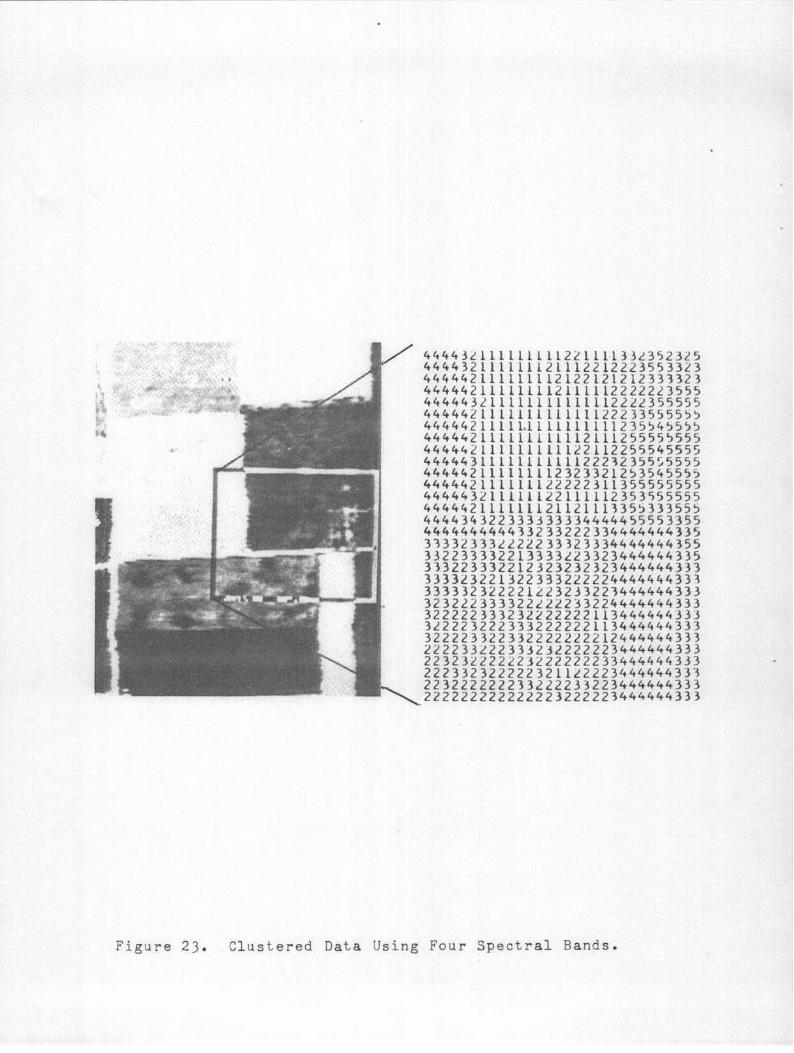
Figure 23 shows the result of applying such a clustering technique to sOme multispectral data. The algorithm was instructed to form five clusters. A comparison of the clustering results with the data in image form shows that the clusters. indeed were assoc­iated with individual fields. Cluster four, for exam­ple, was associated with fields in the upper left and lower right. Clusters two and three with the field in the lower left and so on. Such a technique is useful to speed the training phase of the classifier by aiding the human operator in obtaining points grouped accordinq to the class that they originate from. The statistics of each cluster point can be immediate­ly computed from the cluster results so that decision boundaries are quickly established. The operator is thus relieved of the necessity of locating and separ­ating individual resolution points of fields for training each class.

The value of sqch a procedure is even greater in cases where large groups of points associated with the same class and located contiguous to one another are not present as they were in Figure 23. Figure 24 shows the result of clusterinq data for a soils mapp­ing classification. Here it would be more difficult. to select samples associated with specific soil types. As a result of the clustering, the operator has only to associate the soil type with each cluster point and training samples are immediately available for fur­ther processing.

Such clustering techniques are very useful in the training phase of utilization of a supervised classifier. The specific steps to be followed in training a classifier are dependent not only upon the data set but also upon the users informational needs. The following steps, which are similar to the ones used in the ERTS data analysis example, are rather typical:

-22-

1. Make available to the clustering algorithm every mth sample of every nth scanline. It is.ordinar~ly not necessary to cluster every po~nt and ~ndeed to do so unnecessarily wastes computer resources. The values of m and n needed in each situation are a matter of judge­~ent depending on the availability of comput-1ng resources and how the classes dis-tribute themselves over the data set to be analyzed.

2. Examine the results of the clustering to establish first that each of the clusters is sufficiently separable from the others and second that the clusters are associated with same class of material of interest.

3. Manually select additional training sets as may be needed to treat special situations.

4. Fram this point the statistics of each class may be computed from appropriate clusters and the classification.

Section VIII: ON THE SPEED AND COST OF DATA PROCESSING

Let us return to the question of processing speed and economics. It was mentioned earlier that, in order to deal with the large volume of data, special care must be exercised in the choice of method such that one of great throughput capability would be possible. It was also pointed out that the aspects of simplicity and processing of a parallel nature contribute in this direction. Perhaps it is now more apparent why the multispectral approach is valuable in this respect. All of the data relevent to a single resolution ele­ment on the ground is collected and available for processing at the same instant of time. Thus, rather than requiring the processing of several different images (e.g. from several different spectral bands) one must only process a single vector at a time. The mathematics and algorithms of multivariant analysis are thus immediately available and implementations of this mathematics in parallel processor form are known and well understood.

So far implementations of the classification algorithm used in the above examples have been made on general-purpose digital computers, such as was used to generate the above examples, and special purpo.se analog processors. * Sane work has begun in

*The SPARC Processor of the Environmental Research In-stitute of Michigan is an outstanding example of this.

-23-

looking at operational implementations of the processing algorithms which have been studied under research circum­stances. Both software techniques, such as "table look-up" implementations of classifiers,l5 and advanced hardware techniques l ,,17 could produce operational processing cost reductions of several orders of magnitude over those processing costs ot" general purpose digital computers and the highly flexible software necessary in the research environment. Results on quantitative camparisons between processing approaches le and their costs are not yet abundant.

Section IX: ON mE USE OF SPATIAL INFORMATION

So far we have discussed the use of spectral and temporal variations to derive information from measure­ments of electromagnetic energy arriving at the sensor. It is also possible to utilize spatial information within the multispectral approach in order to further increase the amount and accuracy of· information that can be derived. One such approach to accomplish this is the so-called per field classifier. 19 ,20,21 In essence, the use of spatial information in this approach results from the fact that points in a near vicinity to one another are likely to be members of the same class. Consider, for example, the situation as shown in Fiqure 23. Here one might be willing to say, "I don't know what all the points in cluster number 4 are, but whatever they are I am willing to say that they are all members of the same class. What is this class?" Thus, in this case one sees a "situation where a set of points rather than an individual point is avail-able for a single classification. In essence then, the mathematics of the situation permits one to use this set of points to estimate the statistical distribution function of the points. This estimated distribution can then be campared with the distribution function of the points. This estimated distribution can then be compared with the distribution of each training set to decide upon the proper classification. * Thus, one is comparing a point set to a set of distributions as campared to comparing a single (vector) point to a set of distributions. As may be seen in the reference,2o a generally higher classification accuracy is achieved by this mode. One does have the preliminary problem, though, of grouping all points into point sets. This may be either accomplished by a boundary drawing algorithml ' or through the use of clustering it­self as shown in Fiqure 23.

* The mean and variance of this estimated distribution correspond roughly to tone and texture used by the human photo interpreter.

-24-

Section X: DATA PREPROCESSING STEPS

Having now treated the portion of the system involv­ing data analysis (see Figure 2) it is appropriate that. we ret.urn briefly t.o t.he preprocessing sect.ion of t.he syst.em. Depending upon t.he type of informat.ion needed and therefore the t.ype of analysis to be used, there are ~ large number of possible dat.a preparation or preprocess-1ng st.eps which prove necessary of helpful. The t.able given below enumerates some of them.

CALIBRATION

Radiomet.ric (intensity) Manipulation Geometric Manipulation

ENHANCEMENT

Spat.ial Frequency Operations Mult.ivariate Transformat.ions ConVOlutional Filt.ering

MULTI-IMAGE OPERATIONS

Inter-image Addit.ion Subtraction, etc. Inter-image Registration

DATA PRESENTATION

Generally, on board the sensor platform, as was previously mentioned, various types of calibration information are derived. Thus, a possible preprocess­ing step is to apply this calibration information to the data. This may take the form of radiometric calibration in which correct.ions are made for variations in the at­mospheric transmission, system gain, sensor aging and the like. A second type of calibration is that associated wit.h the geometry of the image. Usually it is necessary to make intra-image corrections of both a relative and an absolute type. For example, in the ERTS-l MSS images a type of skew distortion arises because t.he earth is rotating beneat.h the satellite during the period of time that a single frame is being sensed. Thus, a correction must be applied on an intra-image basis in order that individual resolution elements will have the proper relative location with respect to one another.

On the other hand, it may be necessary for storage and retrieval purposes to est.ablish the location of each resot'ution element relative to an earth-oriented coordinate

-25-

system on a more absolute basis. An example of such an operation is the so-called scene correction or precision image processing done with the ERTS-l imagery.

Another example of a calibration type of preprocess­ing is the so-called angle correction process. The amount of radiation which is reflected from a given scene area is dependent upon both the angle from which it is illuminated and the angle from which it is viewed. 22 This problem has been long known to the field of photo­interpretation in terms of the so-called image "hot spot". It is possible to process the data in such a way that the hot spot appears to have disappeared. Unfortunately, since the angle affect depends not only upon the illumination angle and view angle but also upon the scene material on the ground, it is generally not possible to process the data to a point of being radiometrically correct. In short a suitable approach to this problem from a radiometric standpoint is not known at this time.

In recent years a considerable amount of work has been done in the image enhancement area. Spatial frequency operations have been widely studied for such purposes as 23 enhancing boundaries in the imagery, removing low-frequency shading affects, correcting for distortions introduced by the data transmission system, removing single frequency coherent noise and the like. Enhancement by carrying out a multivariant transformation on multispectral imagery for enhancement pur~oses has also be~n examined.

. Multi-image operations are also some times necessary and desirable. One of the most important multi-tmage operations is that of achieving registration between two images collected over the same scene at different times or in different portions of the electromagnetic spectrum. This problem has great importance and it has been extensively studied. Techniques today tElnd to fall into two broad classes. The first is th6se inVOlving primarily optical techniques developed primarily in the field of photogrammetry usihg image projedtion techniques and ancillary data derived from system characteristics and operation. The second approach to the problem differs from this in that registration is aChieved generally through point by point processing and utilizing . information derived from the data itself. TWo-dimensional­image correlation is a common approach in this latter case.2Itl25,2&

-26-

Once having achieved image registration, access is gained to temporal information in terms of tech­niques described earlier. In addition, inter-image manipulation for the purpose of noise minimization, for example, by adding two images of the same area gathered at nearly the same time and for highlight­ing certain types of changes in the imagery through ratioing22 of registered images may also prove helpful.

A very important additional tape of data pre­processing is data compression. Data compression may be desirable to minimize the data volume problem either in terms of necessity for data transmission through a given link or in terms of minimizing the data storage and retrieval problem. Relatively

.simple compression techniques based on both spectral and spatial redundancy appear to be possible at this time. Compression ratios of 5 or 10 to 1 without loss of essential information in the data appear within reach at this time. 27 ,2.

A most important area and one receiving con­siderable attention at this time is that of data display. Since the quantity of data to be dealt with is typically so large, methods by which to vtew it are most important in both pictorially and numerically oriented systems. Various .types of viewers and image misplay systems including those involving color in various ways are being constructed, marketed, and used especially in the pictorially oriented field. Though of perhaps less central importance to the numerically oriented field, image data display systems are utilized as effective means by which to monitor processing system performance and to interact with it. The most difficult operation of merging ancillary data with the data stream is often best done this way. In addition, various types of printers and plotters are used to present results in map form for the user's purposes.

Section XI: CONCLUSION

In summary, pattern recognition and the multi­spectral approach have been described as an analysis procedure which will prove useful in coping with the large quantities of data to be gathered by earth resources sensors. This approach was illustrated

-27-

with two examples, one using airborne scanner data another using multispectral data gathered on a spaceborne platform. The manner in which spatial and temporal variations in the data can be utilized to increase the quantity and accuracy of informa­tion derivable has also been described. Training procedures were identified as an important step in using this pattern recognition approach and the use of clustering to aid in this process was described. And finally, possible types of preprocessing steps for both pictorially and numerically oriented systems were summarized.

In addition to data volume, remote sensing information systems in the earth resources disciplines are characterized by the large number and variety of users of the information to be generated. Many d~fferent techniques will be needed working together to supply the information needed by all users.

We hope the reader will find the material of this Information Note helpful not only in understanding the multispectral machine processing approach but in seeing its relationship to other older and more well-established techniques and in visualizing how all can contribute to meeting their varied user needs.

•

-28-

1. Holmes, R.A. and R.B. MacDonald. 1969. The Physical Basis of System Design for Remote Sensing in Agriculture. Proc. of the IEEE. Vol. 57, No.4, pp. 629-639.

2. Laboratory for Agricultural Remote Sensing (LARS). 1967. Inter retation of Remote Mu1tis of Agricultural Crops. Research Bu , Annual Report, Volume 1. Purdue University Agricul­tural Experiment Station, Lafayette, Indiana.

3. Laboratory for Agricultural Remote Sensing (LARS). 1967. Remote MUltis~ectral Sensing in Agriculture. Researcfi Bulletin 83 , Annual Report Volume fl. Purdue University Agricultural Experiment Station, Lafayette, Indiana.

4. Fu, K.S., D.A. 1969. Information Agricultural Data. pp. 639-653.

Landgrebe, and T.L. Phillips. processing of Remotely Sensed Prac. of the IEEE, Vol. 57, No.4,

5. Nilsson, N.J. 1965. Learning Machines. ,McGraw-Hill, New York.

6. Nagy, G. Recognition. pp. 836-862.

1968. State of the Art in Pattern Proc. of the IEEE, Vol. 56, No.5,

7. Landgrebe, D.A. and LARS Staff. 1967. Automatic Identification and Classification of Wheat by Remote Sensing. Purdue Agricultural Experiment Station Research Progress Report 279.

8. Landgrebe, D.A., R.M. Hoffer, F.E. Goodrick, and Staff. 1972. An Early Analysis of ERTS-l Data. Proc. of the ERTS-1 S?;tOSium. Goddard Space Flight Center, Greenbelt, Mar and, Septmeber 29.

9. Anuta, P.E. and R.B. MacDonald. 1971. Crop Surveys from Mu1tiband Satellite Photography Using Digital Techniques. Remote Sensing of the Environ­ment 2(1), pp. 53-67.

10. Anuta, P.E., S.J. Kristof, D.W. Levandowski, T.L. Phillips, and R.B. MacDonald. 1971. Crop, Soil, and Geological Mapping from Digitized Multi­spectral Satellite Photography. Proc. of the 7th International symposium on Remote Sensing of the

-29-

Environment, Inst. of Science and Technology, univ. of Michigan, PP. 1983-2016.

11. Ball, G.H. 1965. Data Analysis in the Social Sciences. What About the Details? IEEE Proc. Fall Joint Computer Conference, 27 Part 1, pp. 533-560.

12. Friedman, H.P. and J. Rubon. 1967. On Some Invariant Criteria for Grouping Data. American Statistical Association Journal 62:1159-1178.

13. Haralick, R.M. and G.L. Kelly. 1969. Pattern Recgonition with Measurement Space and Spatial Clustering for Multiple Images. Proc. of the IEEE, Vol. 57, No.4, pp. 654-665.

14. Wacker, A.G. and D.A. Landgrebe. 1970. Boundaries in Multispectral Imagery by· Clustering. IEEE Symposium on Adaitive Processes (9t:Q.) Decision and Control, pp. X14. -X14.8.

15. Eppler, W.G., C.A. Helmke, and R.H. Evans. 1971. Table Look-Up Approach to Pattern Recognition. Seventh International S osium on Remote Sensing o t e Env1ronment, Ann Ar or, c 19an. May.

16. Preston, K., Jr. 1972. A Comparison of Analog and Digital Techniques for Pattern Recog­nition. Proc. of the IEEE, Vol. 60, No. 10, October.

17. Bouknight, W.J., S.A. Denenberg, D.E. McIntyre, J.M. Randal, A.H. Sameh, and D.L. Slotnick. 1972. The Illiac IV System. Proc. of the IEEE, Vol. 60, No.4, April.

18. Joseph, R.D., R.G. Runge and S.S. Viglione. 1969. Design of a Satellite-Born Pattern Classifier. Symposium on Information Processing, Purdue University, Lafayette, Indiana.

19. Landgrebe, D.A. 1969. Automatic Processing of Earth Resource D~a. Proc. of the 2nd Annual Earth Resource Aircraft Program Status Review, NASA/Manned Spacecraft Center, Housto:Q" Texas.

20. Wacker, A.G. to Classification.

1972. Minimum Distance Approach Ph.D. Thesis, Purdue University.

-30-

21. Wacker, A.G. and D.A. Landgrebe. 1972. Minimum Distance Classification in Remote~nsing. First Canadian Symposium for Remote Sensing, Ottawa, Canada.

22. Kriegler, F., W. Malila, R. Nalepka and w. Richardson. 1969. Preprocessing Transformations and Their Effects on Multispectral Recognition: Sixth Symposium on Remote Sensing of the Environment, Ann Arbor, Michigan. October.

23. Billingsly, F.C. 1970. Applications of Digital Image Processing. Applied Optics. Vol. 9, No.2, February.

24. Anuta, P.E. 1969. Digital Registration of Multispectral Video Imagery. Society of Photo Optical Instrumentation Engineers, Vol. 7, No.6.

25. Anuta, P.E. 1970. Spatial Registration of Multispectral and Multitemporal Digital Imagery Using Fast Fourier Transform Techniques. IEEE Transactions on Geoscience Electronics, VoI:""GE, No. 4, pp. 353-368.

26. Lillestrand, R.L. 1972. Techniques for Change Detection. IEEE Transactions on Computers, Vol. C-2l, NQ. 7. July.

27. Ready, P.J., P.A. Wintz, S.J. Whitsitt and D.A. Landgrebe. 1971. Effects of Compression and Random Noise on Multispectral Data. Proc. of the 7th International Symposium on Rem~ Sensing of the Environment. Inst. of Science and Technology, univ. of Michigan, pp. 1321-1342.

28. Ready, P.J. 1972. Multispectral Data Compression Through Transform Coding and Block Quantization. Ph.D. Thesis, Purdue University. June.

" 0'"

.~ . • :.0

WAV£L£NGfH ..... C-W

Figure 1. The Electromagnetic Spectrum.

Earth Ancillary Data

LARS/Purdue

Figure 2. Organization of an Earth Survey System.

Figure 3.

E Radiation from Atmosphere

E Rodloflon_ -- -from Ground

\ \

---8 Reflected / // / I Sunlight / I

/ Direct / / ( / Sun li9';Y I I

/ / / I

/ /'Oust and: I

/ : Par.ticle~: I ,/ <Cattered I

'- Sunlight I

I -'R~d E Radiation --r from Vegetation

I I I I

.... ...J Reflected

Sunlight

Reflected (R) and Emitted (E) Radiation Energy Exchange in a Natural Environment.

I Sensor 1-1 ----If Preprocessing .... 1 --4\ Form . . lmaoe I---~I Analysis 1----- Results

Image Orientation

I Sensor 1 [ Preprocessing : I A I . 1 I na y5IS r Results

I T , Form Monitor

Image and

Analysis

Numerical Orientation

Figure 4. Organization of Image and Numerically Oriented Systems.

. 38-.44/oLm .41-.47ftm

.4S-;52/oLm .48-.5s,.m .SS-.64ftm

.71-.?9,om .S5-.S9,om

Figure S. Multispectral Photography of Color Cards.

.4-.7~rn .7 - . 9~rn 4.5 - 5.5~rn (Artistts Concept)

Figure 6. Multispectral Response of Corn Alfalfa, Stubble, and Bare Soil.

Response - Vegetation Soil

•...... Water

10

Wavelength, fLm

Response

A2 Vegetation

•

• Water

• Soil

Response, AI

Figure 7. Spectral Data ln Two-Dimensional Feature Space.

Response, A2

100 days

30 days

, • Soybeans '0 Corn

Response, AI

Figure 8. Temporal Change in Two-Dimensional Feature Space.

Response,

~2

Figure 9.

Response,

~2

Figure 10.

Soybeans l1

l1 l1 6

l1

• u + Wheat

0 + + 0 0 +

0 +

0

Corn

Response, ><1

Samples in Two-Dimensional Feature Space.

Soybeans l1

6 A .....

6 6

0

0 0 • 0

0

Corn

Wheat

+ + + +

+

Response, ><1

Minimum Distance to Means Classification.

(a)

Figure 11.

Decide Wheat Decide

~ r-~::: __ ---:--.... __ ~AlfOlto --- 2 / GfiJI / I I / ~2

11 -1

/ ;' /.///j 1/ / I /"/ / i .

( j ij /11

" 'Decide/ / / Ile---/ / Corn / ---=

I / / / -1 /

(b)

Density Functions and Decision Regions for a Statistical Approach.

...... * ~~\-------­

Ground Resolution Patch

Figure 12. An Airborne Multispectral Scanner.

.. • < .t '" ~'

.' '. , • , ". •

" .• 1 \, ~ r.,''f' , , ~ .. ' ),;" .. ,wt

~:'~f._ ~, .

" " o

'" , N ....

" " N .... , '" '"

" " '" '" , N

'"

" " ..,. ..,.

0 ..,.

o " o .c Q.

~ .... <

'" .c " 00 ~

'" M

'" > .. ~

~ :> 0 ... ~ .... ~

" ~ '" '" M

'" ~ :> 00 .... ...

Air Photo Row Crops (Corn & Soybeans)

" .' .. ,. ::

...

.. ',. ."

': .. ~ . ' .. . . ... . , ' ...

. ¥- .

. . . ,"",

.. ,~ i f.k . . '

I ,' .f

I

I

Cereal Grains (Wheat & Oats)

Figure 14. Spectral Pattern Recognition of Row Crops and Cereal Grains.

100 96%

5 90 o

~ 80 -. • 70

" i .0 8 so ~ 40

if '0 20

'0 o

.. % '00"1. 9'% 92%

84% 8'%

8.%

Row Wheal Ools Paslure Hoy Bore fbod, Trees Wafer Crops So"

Figure 15 . Classification Results for Test Samples.

Figure 16. Simulated Color Infrared of Tcxoma Frame.

•

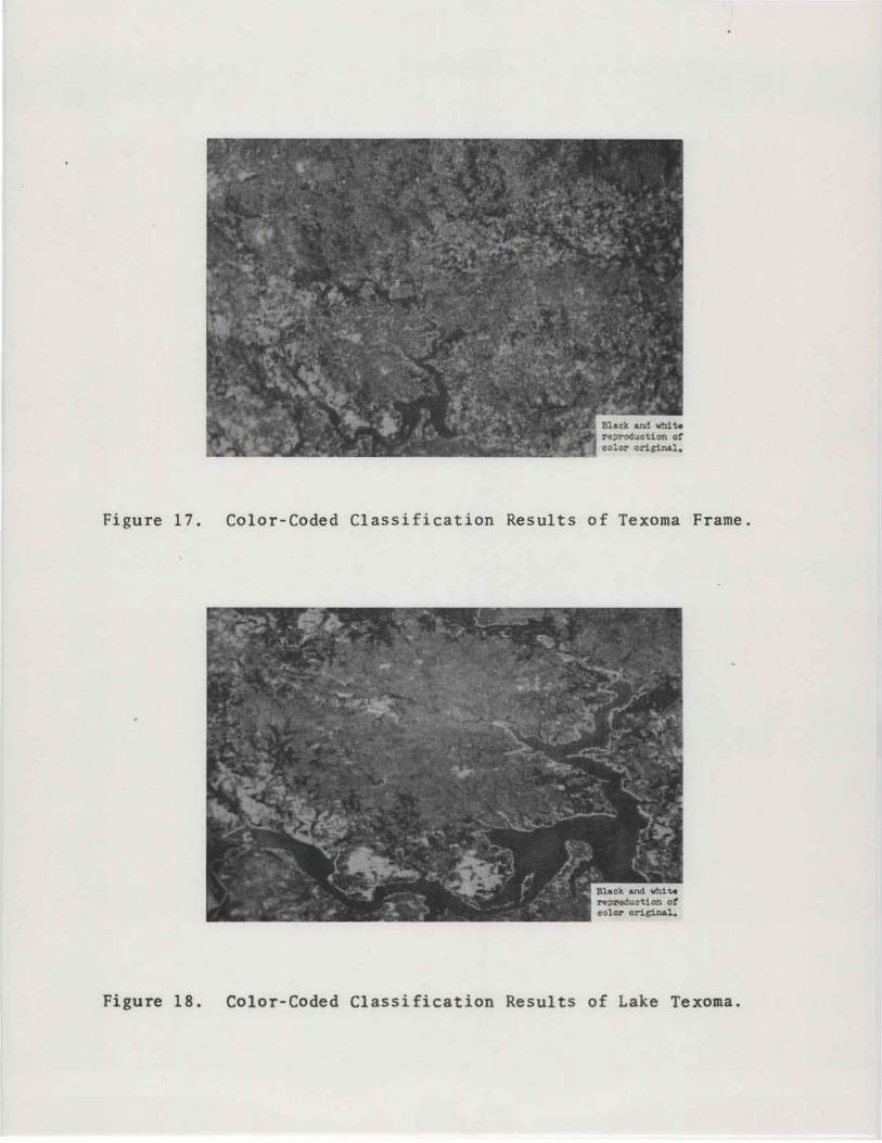
Figure 17.

Figure 18.

r e;rod\l"Uoa or color orl~.

Color-Coded Classification Results of Texoma Frame.

COlor-Coded Classification Results of Lake Texoma.

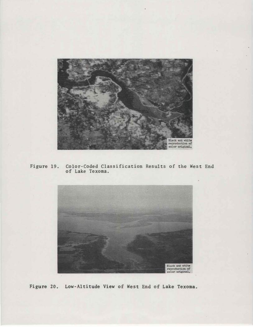
Figure 19. Color-Coded Classification Results of the West End of Lake Texoma.

Figure 20. Low-Altitude View of West End of Lake Texoma.

Rnponse . >0,

Figure 21. Samples in Two-Dimensional Feature Space.

Cka.r I

Figure 22. Clustering in Two-Dimensional Feature Space.

, \. ~ ••

•

44443illllllll12~111133l352325 44443 2 1111111 21 11 22 122 23553323 444442111111112122121212331323 44444 2 111111112111112 222223555 4444432111111111111122L2355555 444442Llllllllllll1222335555~~ 4444421111hllllllLll1235~4~5~~ 444442111l1l1111121112 5555~555 44444~111llll11122112255545555 4444431Lllllllll1222l2355~5555 4444421111111123233212~3545555 44444211111112222 23 11 355555555 4444432111il122l1111235]S55555 444442lllllllZlllllll35'33355' 444434322333333334444455553355 444444444433233 2223344 44444335 )3332333£222233323334444444355 3J22333322l3333,23323444444335 333223332212323232323444444333 33332322l3223l322222444444433l 333332322221~23233223444444333 3232l2333322L22233224444444333 322222331232~2222211344444433J 3~2223222333222222113444444333 322223322332222222212444444333 222233L2233j2j2222223444444333 223232222l2J2222222334444443J3 22233232222232ll,222344444433' 223222222213ll2231Z23444444333 22222222222222322222344444433)

Figure 23 . Clustered Data Using Four Spectr al Bands .

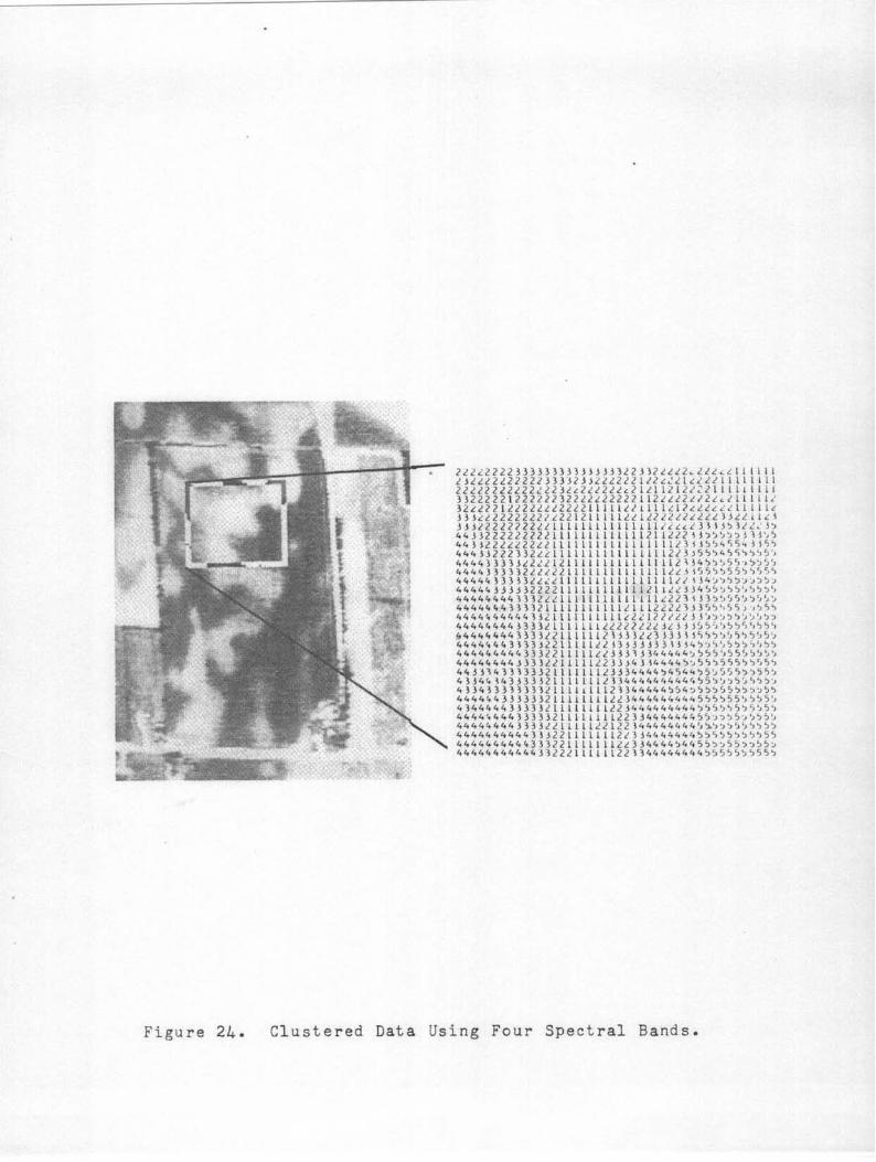
Fig u re 24. Cl u stered Data Using Four Spectral Bands .