Embed Size (px)
Citation preview

THE UNIVERSITY OF NAIROBI
SCHOOL OF COMPUTING AND INFORMATICS
MACHINE LEARNING TECHNIQUES FOR OPTIMIZING THE PROVISION OF STORAGE
RESOURCES IN CLOUD COMPUTING
INFRASTRUCTURE AS A SERVICE (IaaS): A COMPARATIVE STUDY
BY
EDGAR OTIENO ADDERO
A RESEARCH PROJECT REPORT SUBMITTED IN PARTIAL FULFILLMENT OF THE
REQUIREMENTS FOR THE AWARD OF THE DEGREE OF MASTERS OF SCIENCE IN
COMPUTER SCIENCE OF THE UNIVERSITY OF NAIROBI.
OCTOBER 2014
1
DECLARATION
This research project report is my original work and has not been presented for any award in any
other University.
EDGAR OTIENO ADDERO DATE…………………………
P56/61437/2010
This research project report has been submitted in partial fulfillment of the requirements of the
Masters of Science in Computer Science of The University of Nairobi with my approval as the
University Supervisor.
Dr. ELISHA T. OPIYO OMULO DATE…………………………
Senior Lecturer
School of Computing and Informatics
University of Nairobi

2
AKNOWLEDGEMENT
I wish to express my appreciation to Dr. Elisha Opiyo, who served as my supervisor, for all the
support and guidance. I would also like to appreciate Ms. Christine Ronge for her guidance and
contributions. Many thanks are due also to other members of the panel and review committee
Mr. Lawrence Muchemi, Dr. Robert Oboko who provided the technical guidance that I so much
needed though this research. My thanks and gratitude is due also to my parents for their
encouragement and patience without which this work would not have been possible. My
gratitude also goes to my colleagues for their encouragement and insights during this project.
Above all I thank God the almighty for granting me good health and the spirit to work on this
project.

3
ABSTRACT
Cloud computing is a very popular field at present which is growing very fast and the future of
the field seems really wide. With progressive spotlight on cloud computing as a possible solution
for a flexible, on-demand computing infrastructure for lots of applications, many companies and
unions have started using it. Obviously, cloud computing has been recognized as a model for
supporting infrastructure, platform and software services. Within cloud systems, massive
distributed data center infrastructure, virtualized physical resources, virtualized middleware
platform such as VMware as well as applications are all being provided and consumed as
services. The cloud clients should get good and reliable services from a provider and the provider
should allocate the resources in a proper way so as to render good services to a client. This
brings about the problem of optimization where clients request for more services than they
actually require leading to wastage of the cloud storage resource .This demands for optimization
both on the part of the client and the cloud service provider. This has lead to increased research
in the various techniques that can be used for resource allocation within cloud services. This
research focuses on the analysis of machine learning as a technique that can be used to predict
the cloud storage service request patterns from the clients. The research focuses on a review of
machine learning as a technique that can be used to predict and therefore optimize the user
storage resource demand and usage for the case of cloud computing storage IaaS. Data on cloud
storage resource usage was subjected to experiments using machine learning techniques so as to
determine which give the most accurate prediction. Some of these machine learning techniques
to be reviewed in this research include linear regression, artificial neural networks (ANN),
support vector machines (SVM).From the experiments done in this research, it can be concluded
that the use of support vector machine algorithm (SVM) proves to be the best algorithm for
learning the storage resource usage patterns and predicting their future usage so as to enable
better resource budgeting.

4
LIST OF ABREVIATIONS
IaaS-Infrastructure as a Service
PaaS-Platform as a Service
SaaS-Software as a Service
API-application programming interface
WWW-world wide web
RTE-run time environment
FLOP-floating point operations per second
ML-machine learning
SVM-support vector machine
DNS-domain name server
SLA-Service Level Agreements
AMAZON E2C-Amazon elastic compute cloud
CRAIG-cloud resource allocation game
SVM-support vector machine
CSV-comma separated values

5
Table of Contents
List of figures ................................................................................................................................................ 7
List of tables .................................................................................................................................................. 8
CHAPTER ONE : INTRODUCTION .......................................................................................................... 9
1.0 Background ......................................................................................................................................... 9
1.1 Problem statement ............................................................................................................................. 12
1.2 The goal of the study ......................................................................................................................... 13
1.2.1 Specific objectives ..................................................................................................................... 13
1.3 Research question ............................................................................................................................. 13
1.4 Scope of the study ............................................................................................................................. 13
1.5 Significance....................................................................................................................................... 14
1.6 Contributions..................................................................................................................................... 14
1.7 Organization of the report ..................................................................................................................... 14
CHAPTER TWO : LITERATURE REVIEW ............................................................................................ 15
2.0 Introduction ....................................................................................................................................... 15
2.1 Cloud computing ............................................................................................................................... 16
2.1.3 Cloud deployments models ........................................................................................................ 19
2.3.5 Application of supervised machine learning techniques in resource management .................... 49
2.3.6 Tools used in machine learning and predictive modeling .......................................................... 52
2.5 summary of literature review ............................................................................................................ 54
2.6 Conceptual model ............................................................................................................................. 55
CHAPTER THREE : METHODOLOGY .................................................................................................. 56
3.0 Introduction ....................................................................................................................................... 56
3.1 Research design ................................................................................................................................ 56
3.1.2 Selection of variables/Type of data required ............................................................................. 56
3.1.3 Type of study ............................................................................................................................. 57
3.1.5 Data Collection of training data ................................................................................................. 58
3.1.5.1 Data collection instruments ..................................................................................................... 58
3.1.5.2 Research Sample design .......................................................................................................... 58
3.1.5.2.1 Research population ............................................................................................................. 58
3.1.7 Preparation of the data for training ............................................................................................ 60

6
3.1.8 Data Analysis ............................................................................................................................. 63
3.1.8.1 Processing of prediction accuracy data ................................................................................... 63
3.1.8.1 Comparison of the Machine learning techniques .................................................................... 64
CHAPTER FOUR : RESULTS ANALYSIS AND EVALUATION ......................................................... 65
4.0 Introduction ....................................................................................................................................... 65
4.1 Data sets collected ............................................................................................................................. 65
4.1.1 Data set collected in tabular format ............................................................................................... 65
4.1.2 Graphical representation of data for Client resource(Storage) usage over six months .................. 66
4.1.3 Resource requests verses the usage ................................................................................................ 66
4.2 Results of accuracy of prediction of resource usage ......................................................................... 67
4.2.1 Tabular presentation ................................................................................................................... 67
4.2.2 Graphical presentation of results ................................................................................................ 67
4.3 Comparison of accuracy of the predictions by the various algorithms ............................................. 70
4.4 Limitations and challenges................................................................................................................ 71
CHAPTER FIVE : CONCLUSION AND RECOMMENDATIONS ........................................................ 72
5.1 Conclusion ........................................................................................................................................ 72
5.2 Recommendations ............................................................................................................................. 72
5.3 Further work...................................................................................................................................... 72
REFFERENCES ......................................................................................................................................... 73
APPENDICES ............................................................................................................................................ 76
Appendix 1:Screenshots for results ......................................................................................................... 76
Comparative usage over six months ................................................................................................... 76
Actual versus predicted usage over six months .................................................................................. 77
Appendix 2: Sample questions to Safaricom ltd. engineers .................................................................... 78
Appendix 3:Sample dataset experimented upon ..................................................................................... 79
Appendix 4:DTREG user manual screen shots ....................................................................................... 87

7
List of figures
Figure 1-Cloud systems architecture .......................................................................................................... 18
Figure 2-Process for using a machine learning technique to predict client storage resource usage. ........ 55
Figure 3-Request verses usage over six months ......................................................................................... 66
Figure 4: Resource requested versus usage ............................................................................................... 67
Figure 5: Coefficient of variation ................................................................................................................ 68
Figure 6: Root mean square error ............................................................................................................... 68
Figure 7: Mean percentage error ................................................................................................................ 69
Figure 8: Correlation between actual and predicted values ....................................................................... 69
Figure 9-DTREG-main screen ...................................................................................................................... 87
Figure 10-DTREG screen for setting prefferences ...................................................................................... 88
Figure 11-DTREG screen for loading training data files and specifying storage location for outputs ........ 89
Figure 12-DTREG screen for selecting the prediction model ...................................................................... 90
Figure 13-DTREG screen for setting model variables ................................................................................. 92
Figure 14-DTREG screen for model creation .............................................................................................. 93
Figure 15-DTREG screen for results report ................................................................................................. 93

8
List of tables
Table 1: Storage allocation policies for Amazon S3 .................................................................................... 31
Table 2: Storage pricing for Rackspace ....................................................................................................... 32
Table 3: Storage allocation for Google computer ....................................................................................... 33
Table 4: Storage allocation policy for Windows Azure ............................................................................... 33
Table 5: Cloud storage policy for GOGRID .................................................................................................. 36
Table 6: Packages and Pricing for storage for Safaricom Ltd. ..................................................................... 38
Table 7: Packaging and Pricing for cloud backup service for safaricom Ltd. .............................................. 40
Table 8-classification of client requests for storage on a six month cumulative basis ............................... 60
Table 9-classification of cloud storage service request in GigaBytes ......................................................... 60
Table 10-measures of accuracy for various learning model ....................................................................... 67
9
CHAPTER ONE : INTRODUCTION
1.0 Background
Cloud computing is a model for enabling ubiquitous, convenient, on-demand network access to a
shared pool of configurable computing resources such as networks, servers, storage, applications,
and services that can be rapidly provisioned and released with minimal management effort or
service provider interaction (NIST).
Cloud Computing has become one of the popular buzzwords in the IT area after Web2.0. This is
not a new technology, but the concept that binds different existing technologies altogether
including Grid Computing, Utility Computing, distributed system, virtualization and other
mature technique.
Cloud computing systems provide environments to enables resource provision in terms of
scalable infrastructures, middleware, application development platforms and value-added
business applications. Software as a Service (SaaS), Platform as a Service (PaaS) and
Infrastructure as a Service (IaaS) are three basic service layer.
SaaS: The capability provided to the consumer is to use the provider’s applications running on a
cloud infrastructure. The applications are accessible from various client devices through either a
thin client interface, such as a web browser (e.g., web-based email), or a program interface. The
consumer does not manage or control the underlying cloud infrastructure including network,
servers, operating systems, storage, or even individual application capabilities, with the possible
exception of limited user-specific application configuration settings (NIST).
PaaS: The capability provided to the consumer is to deploy onto the cloud infrastructure
consumer-created or acquired applications created using programming languages, libraries,
services, and tools supported by the provider. The consumer does not manage or control the
underlying cloud infrastructure including network, servers, operating systems, or storage, but has
control over the deployed applications and possibly configuration settings for the application-
hosting environment (NIST).

10
IaaS: The capability provided to the consumer is to provision processing, storage, networks, and
other fundamental computing resources where the consumer is able to deploy and run arbitrary
software, which can include operating systems and applications. The consumer does not manage
or control the underlying cloud infrastructure but has control over operating systems, storage,
and deployed applications; and possibly limited control of select networking components
(NIST).
Examples of infrastructure services provider on a global scale include Rackspace, GoGrid,
Amazon EC2, Microsoft Azure Platform, Terremark Cloud Storage, and more. Infrastructure
services address the problem of properly equipping data centers by assuring storage computing
power when needed.
Various resources are available within the cloud computing environment. Resource consumption
by an application in the form of CPU time, disk space, amount of memory and network
bandwidth is a useful set of information when available before allocating resources. The need to
know resource consumption has the benefit of helping cloud service providers in resource
optimization
In cloud computing, Resource Allocation is the process of assigning available resources to the
needed cloud applications over the internet. Resource allocation starves services if the allocation
is not managed precisely. Resource provisioning solves that problem by allowing the service
providers to manage the resources for each individual module (mahendra et. al, 2013).
An optimal Resource Allocation Strategy should avoid the following criteria i.e. Resource
Contention in which demand exceeds supply for a shared resource, such as memory, CPU,
network or storage. In modern IT, where cost cuts are the norm, addressing resource contention
is a top priority. The main concern with resource contention is the performance degradation that
occurs as a result. Second Criteria is Scarcity of Resource which happens when there are limited
resources and the demand for resources is high. In such situation user can not avail facility of
resource. Third criteria are Resource Fragmentation –In these criteria resources are isolated.
There would be enough resources but cannot allocate it to the needed application due to
fragmentation into small entities. If fragmentation is done into big entities then we can use it

11
optimum. Forth criteria is Over Provisioning – Over provisioning arises when the application
gets surplus resources than the demanded one. Due to this, the investment is high and revenue is
low. The fifth criterion is Under Provisioning, which occurs when the application is assigned
with fewer numbers of resources than it demanded (Mahendra et. al, 2013).
In the Kenyan context, Safaricom limited is one of the companies offering cloud computing
services. With cloud services, businesses of all sizes are able to reap the benefits of not having to
deploy physical infrastructure in their premises such as file and e-mail servers, storage systems
and software. Access to these IT resources means hassle-free collaboration between business
partners and employees by using simple online applications. The cloud services offered by
Safaricom include
Infrastructure as a Service
Data Centre
Storage Services
Platform as a Service
Hosted Applications
Software as a Service
Data Archiving
Backup and Recovery
It is paramount for any organization involved in cloud computing service delivery to identify the
clients’ resource utilization patterns and map this against the available resources so as to be able
to justify their claims when advising clients on their actual cloud resource requirements and in

12
term provide better management of their cloud computing resources. This will enable savings on
the part of the customer since they can be accurately advised on their specific resource
requirements hence more informed resource requests on their part, and on the side of the cloud
service provider, they can be able to optimally plan for the resources available. The aim of this
study is to do a comparative study of machine learning techniques and find out which one yields
the most accurate and optimal prediction for the case of predicting storage resource usage for the
case of Cloud computing IaaS .This could be used to advice clients on their resource usage as
compared to resource requests for the case of IaaS. The solution is to use the usage patterns of
clients in order to suggest the best machine learning technique that can predict client future
storage resource usage and be based on this the provider can achieve better storage resource
investment plan and also be able to advise clients on they can make more efficient resource
acquisition.
1.1 Problem statement
The main problem that is to be addressed by this research is that of over provisioning of
resources which include storage by a cloud IaaS provider [19].Over provisioning arises when the
application gets surplus resources than the demanded ones (vinothina et al.).
As more companies put workloads on Amazon Web Services or other public cloud platforms,
many are paying for more cloud than they need. That over provisioning is the problem. [23].
Over provisioning arises when a client requests for much more resources (processor, RAM and
storage) than what they actually use. This is a problem for organizations offering IaaS in the
sense that some resources go unused. It is also a problem for the clients because they
unknowingly end up paying for more processor and storage resources than they use.

13
1.2 The goal of the study
The project aims to find out the appropriate machine learning techniques to predict client cloud
storage resource usage.
1.2.1 Specific objectives
The specific objectives of the research were as follows:-
i. Identify various machine learning techniques.
ii. Select some machine learning techniques.
iii. Collect real test data.
iv. Simulate additional test data.
v. Run machine learning techniques on the combined test data.
vi. Analyze the results of the machine learning techniques.
vii. Compare the performance of the machine learning techniques.
viii. Complete the report.
1.3 Research question
Which machine learning technique amongst linear regression, support vector machine (SVM)
and artificial neural networks (ANN) gives the best prediction for a user’s storage resource
request verses their usage?
1.4 Scope of the study
The research will be limited to a review of three machine learning techniques that is linear
regression, support vector machine and artificial neural networks and the metrics which will be
used for the evaluation include, Mean Absolute Percentage Error, Root Mean Square Error,
coefficient of variation and comparison between actual verses predicted data.

14
1.5 Significance
Cloud computing is rapidly taking shape all over the world and it is paramount for us to start
thinking how resources are going to be provisioned and allocated in an efficient way based on
some forecasting or prediction mechanism.
On a more specific note, this research will contribute to the body of knowledge that the software
developers for applications that are used for cloud computing resources management and cloud
service providers such as Safaricom Ltd. can benefit from the research by understanding the best
machine learning technique that can be used in prediction of resource usage for the case of cloud
IaaS.
1.6 Contributions
This research has brought to light that indeed machine learning can be used to predict resource
usage for the case of cloud computing storage resource usage and more specifically, Support
Vector Machine (SVM) algorithm is the most suitable for cases similar to that covered in this
research.
1.7 Organization of the report
This research report begins by giving an overview of the cloud computing environment in the
first chapter and the highlights the problem of over provisioning as a major challenge. The
second chapter details an overview of the various machine learning techniques focusing on three,
that is linear regression, support vector and time series algorithms. It also looks at the various
tools that can be used for machine learning. The third chapter gives an overview of how the
research was conducted in terms of the methodology, how the data was prepared and how the
experiments were done. The fourth chapter deals with the analysis of the results from each of the
machine learning algorithms and an analysis of their accuracy in making the predictions for
client resource usage. The fifth chapter is on the conclusions and recommendations that the
researcher came up with after conducting the research

15
CHAPTER TWO : LITERATURE REVIEW
2.0 Introduction
This chapter focuses on cloud computing resources, resource allocation models and methods,
machine learning tools and algorithms, profiling and modeling resource usage, and other related
works. Cloud computing offers three main services which are PaaS, SaaS and Iaas. There is lack
of an appropriate machine learning technique that can be used to predict storage resource
consumption for the case of IaaS cloud computing service. Machine learning can be used to
predict these storage resource usage based on previous client usage patterns. Cloud computing
can be offered using various deployment models and there are various players involved in
offering cloud computing service. These have been conclusively discussed in the literature
review. Various resource allocation models are reviewed so as to get an overview of the various
resources and the methods that are used to allocate these resources. A review on machine
learning is also done so as to give a firm background on the various machine learning algorithms
and modeling techniques, their strengths, weaknesses and applications.
The benefits of this include a better awareness on storage resource usage for future planning on
the part of the organizations Cloud computing services and hence saving on costs as well as
better client advisory on future requirements when they request for storage service requests
thereby saving clients from unnecessary additional costs. The poor performance results produced
by statistical estimation models have flooded the estimation area for over the last decade. Their
inability to handle categorical data, cope with missing data points, spread of data points and most
importantly lack of reasoning capabilities has triggered an increase in the number of studies
using non-traditional methods like machine learning techniques (Yogesh Singh, et. al). The area
of machine learning draws on concepts from diverse fields such as statistics, artificial
intelligence, philosophy, information theory, biology, cognitive science, computational
complexity and control theory. In this case the researcher picked on Safaricom limited as a local
cloud computing service provider and corporate organizations it provides this services to as the
clients for the case of IaaS. If not well managed, a cloud service provider may end up under-
utilizing the available resources on his part and the cloud client may end up paying for more
services than they actually require. This can be both detrimental to the client in terms of
unnecessary cost and to the service provider in terms of resource wastages.
16
2.1 Cloud computing
2.1.1 Definition of cloud computing?
Cloud computing is a model for enabling convenient, on-demand network access to a shared
pool of configurable computing resources (e.g., networks, servers, storage, applications, and
services) that can be rapidly provisioned and released with minimal management effort or
service provider interaction. This cloud model promotes availability and is composed of five
essential characteristics (On-demand self-service, Broad network access, Resource pooling,
Rapid elasticity, Measured Service); three service models (Cloud Software as a Service (SaaS),
Cloud Platform as a Service (PaaS), Cloud Infrastructure as a Service (IaaS)); and, four
deployment models (Private cloud, Community cloud, Public cloud, Hybrid cloud). Key
enabling technologies include: (1) fast wide-area networks, (2) powerful, inexpensive server
computers, and (3) high-performance virtualization for commodity hardware (NIST).
2.1.2 Cloud computing service models
Software as a service (SaaS)
The capability provided to the consumer is to use the provider’s applications running on a cloud
infrastructure. The applications are accessible from various client devices through either a thin
client interface, such as a web browser (e.g., web-based email), or a program interface. The
consumer does not manage or control the underlying cloud infrastructure including network,
servers, operating systems, storage, or even individual application capabilities, with the possible
exception of limited user-specific application configuration settings (NIST).
Platform as a service (PaaS)
The capability provided to the consumer is to deploy onto the cloud infrastructure consumer-
created or acquired applications created using programming languages, libraries, services, and
tools supported by the provider. The consumer does not manage or control the underlying cloud
infrastructure including network, servers, operating systems, or storage, but has control over the

17
deployed applications and possibly configuration settings for the application-hosting
environment (NIST).
With PaaS the following benefits can be achieved:
Develop applications and get to market faster
Deploy new web applications to the cloud in minutes
Reduce complexity with middleware as a service
Infrastructure as a service (IaaS)
IaaS: The capability provided to the consumer is to provision processing, storage, networks, and
other fundamental computing resources where the consumer is able to deploy and run arbitrary
software, which can include operating systems and applications. The consumer does not manage
or control the underlying cloud infrastructure but has control over operating systems, storage,
and deployed applications; and possibly limited control of select networking components
(NIST).

18
Examples of infrastructure services provider include IBM BlueHouse, VMWare, Amazon EC2,
Microsoft Azure Platform, Sun ParaScale Cloud Storage, and more. Infrastructure services
address the problem of properly equipping data centers by assuring computing power when
needed.
Figure 1-Cloud systems architecture
Benefits of cloud computing
The advantages of ―renting‖ these ―virtual resources‖ over traditional on-premise IT includes:
On demand and elastic services—quickly scale up or down
Self-service, automated provisioning and de-provisioning
Reduced costs from economies of scale and resource pooling
Pay-for-use—costs based on metered service usage
In the most basic cloud-service model, providers of IaaS offer computers - physical or (more
often) virtual machines - and other resources. (A hypervisor, such as Xen or KVM, runs the
virtual machines as guests. Pools of hypervisors within the cloud operational support-system can
SaaS
PaaS
IaaS

19
support large numbers of virtual machines and the ability to scale services up and down
according to customers' varying requirements.) IaaS clouds often offer additional resources such
as a virtual-machine disk image library, raw (block) and file-based storage, firewalls, load
balancers, IP addresses, virtual local area networks (VLANs), and software bundles. IaaS cloud
providers supply these resources on-demand from their large pools installed in data centers. For
wide-area connectivity, customers can use either the Internet or carrier clouds (dedicated virtual
private networks).
To deploy their applications, cloud users install operating-system images and their application
software on the cloud infrastructure. In this model, the cloud user patches and maintains the
operating systems and the application software. Cloud providers typically bill IaaS services on a
utility computing basis: cost reflects the amount of resources allocated and consumed.
Examples of IaaS providers include: Amazon EC2, AirVM, Azure Services Platform, DynDNS,
Google Compute Engine, HP Cloud, iland, Joyent, LeaseWeb, Linode, NaviSite, Oracle
Infrastructure as a Service, Rackspace, ReadySpace Cloud Services, ReliaCloud, SAVVIS,
SingleHop, and Terremark
2.1.3 Cloud deployments models
Cloud services can be deployed in different ways, depending on the organizational structure and
the provisioning location. Four deployment models are usually distinguished, namely public,
private, community and hybrid cloud service usage.
Public Cloud
The deployment of a public cloud computing system is characterized on the one hand by the
public availability of the cloud service offering and on the other hand by the public network that
is used to communicate with the cloud service. The cloud services and cloud resources are
procured from very large resource pools that are shared by all end users. These IT factories,
which tend to be specificaly built for running cloud computing systems, provision the resources
precisely according to required quantities. By optimizing operation, support, and maintenance,
20
the cloud provider can achieve significant economies of scale, leading to low prices for cloud
resources. In addition, public cloud portfolios employ techniques for resource optimization;
however, these are transparent for end users and represent a potential threat to the security of the
system. If a cloud provider runs several datacenters, for instance, resources can be assigned in
such a way that the load is uniformly distributed between all centers. Some of the best-known
examples of public cloud systems are Amazon Web Services (AWS) containing the Elastic
Compute Cloud (EC2) and the Simple Storage Service (S3) which form an IaaS cloud offering
and the Google App Engine with provides a PaaS to its customers. The customer relationship
management (CRM) solution Salesforce.com is the best-known example in the area of SaaS
cloud offerings.
Private Cloud
Private cloud computing systems emulate public cloud service offerings within an organization’s
boundaries to make services accessible for one designated organization. Private cloud computing
systems make use of virtualization solutions and focus on consolidating distributed IT services
often within data centers belonging to the company. The chief advantage of these systems is that
the enterprise retains full control over corporate data, security guidelines, and system
performance. In contrast, private cloud offerings are usually not as large-scale as public cloud
offerings resulting in worse economies of scale.
Community Cloud
In a community cloud, organizations with similar requirements share a cloud infrastructure. It
may be understood as a generalization of a private cloud, a private cloud being an infrastructure
which is only accessible by one certain organization.
Hybrid Cloud
A hybrid cloud service deployment model implements the required processes by combining the
cloud services of different cloud computing systems, e.g. private and public cloud services. The
hybrid model is also suitable for enterprises in which the transition to full outsourcing has
already been completed, for instance, to combine community cloud services with public cloud
services.

21
2.1.4 Cloud environment roles
In cloud environments, individual roles can be identified similar to the typical role distribution in
Service Oriented Architectures and in particular in (business oriented) Virtual Organizations. As
the roles relate strongly to the individual business models it is imperative to have a clear
definition of the types of roles involved in order to ensure common understanding.
Cloud Providers offer clouds to the customer – either via dedicated APIs (PaaS), virtual
machines and / or direct access to the resources (IaaS). Hosts of cloud enhanced services (SaaS)
are typically referred to as Service Providers, though there may be ambiguity between the terms
Service Provider and Cloud Provider.
Cloud Resellers aggregate cloud platforms from cloud providers to either provide a larger
resource infrastructure to their customers or to provide enhanced features. This relates to
community clouds in so far as the cloud aggregators may expose a single interface to a merged
cloud infrastructure. They will match the economic benefits of global cloud infrastructures with
the understanding of local customer needs by providing highly customized, enhanced offerings
to local companies (especially SME’s) and world-class applications in important European
industry sectors. Similar to the software and consulting industry, the creation of European cloud
partner ecosystems will provide significant economic opportunities in the application domain –
first, by mapping emerging industry requests into innovative solutions and second by utilizing
these innovative solutions by European companies in the global marketplace.
Cloud Adopters or (Software / Services) Vendors enhance their own services and capabilities
by exploiting cloud platforms from cloud providers or cloud resellers. This enables them to e.g.
provide services that scale to dynamic demands – in particular new business entries who cannot

22
estimate the uptake / demand of their services as yet. The cloud enhanced services thus
effectively become software as a service.
Cloud Consumers or Users make direct use of the cloud capabilities – as opposed to cloud
resellers and cloud adopters, however, not to improve the services and capabilities they offer, but
to make use of the direct results, i.e. either to execute complex computations or to host a flexible
data set. Note that this involves in particular larger enterprises which outsource their in house
infrastructure to reduce cost and efforts.
Cloud Tool Providers do not actually provide cloud capabilities, but supporting tools such as
programming environments, virtual machine management etc.
Cloud Auditor - A third-party (often accredited) that conducts independent assessments of cloud
environments assumes the role of the cloud auditor. The typical responsibilities associated with
this role include the evaluation of security controls, privacy impacts, and performance. The main
purpose of the cloud auditor role is to provide an unbiased assessment (and possible
endorsement) of a cloud environment to help strengthen the trust relationship between cloud
consumers and cloud providers.
Cloud Broker - This role is assumed by a party that assumes the responsibility of managing and
negotiating the usage of cloud services between cloud consumers and cloud providers. Mediation
services provided by cloud brokers include service intermediation, aggregation, and arbitrage.
Cloud Carrier - The party responsible for providing the wire-level connectivity between cloud
consumers and cloud providers assumes the role of the cloud carrier. This role is often assumed
by network and telecommunication providers (NIST).
2.1.5 Cloud characteristics
Cloud computing is a model for enabling ubiquitous, convenient, on-demand network access to a
shared pool of configurable computing resources (e.g., networks, servers, storage, applications,
and services) that can be rapidly provisioned and released with minimal management effort or
service provider interaction. The essential characteristics for cloud computing includes the ones
highlighted below.

23
On-demand self-service. A consumer can unilaterally provision computing capabilities, such as
server time and network storage, as needed automatically without requiring human interaction
with each service provider.
Broad network access. Capabilities are available over the network and accessed through
standard mechanisms that promote use by heterogeneous thin or thick client platforms (e.g.,
mobile phones, tablets, laptops, and workstations).
Resource pooling. The provider’s computing resources are pooled to serve multiple consumers
using a multi-tenant model, with different physical and virtual resources dynamically assigned
and reassigned according to consumer demand. There is a sense of location independence in that
the customer generally has no control or knowledge over the exact location of the provided
resources but may be able to specify location at a higher level of abstraction (e.g., country, state,
or datacenter). Examples of resources include storage, processing, memory, and network
bandwidth.
Rapid elasticity. Capabilities can be elastically provisioned and released, in some cases
automatically, to scale rapidly outward and inward commensurate with demand. To the
consumer, the capabilities available for provisioning often appear to be unlimited and can be
appropriated in any quantity at any time.
Measured service. Cloud systems automatically control and optimize resource use by leveraging
a metering capability1 at some level of abstraction appropriate to the type of service (e.g.,
storage, processing, bandwidth, and active user accounts). Resource usage can be monitored,
controlled, and reported, providing transparency for both the provider and consumer of the
utilized service.
2.1.6 Providers of cloud Infrastructure services
While many are using custom platforms, where they have written their own code to manage their
virtual servers, a lot are using already available frameworks or turnkey solutions to power their
cloud offerings. If an organization is looking to start offering cloud services there is a jungle of

24
different platforms available, both commercial and open source, that can either help it get started
or deliver to the organization a complete solution tailored to fit the organization’s objectives
2.1.6.1 Infrastructure Services offered by cloud Providers
The objective of this section is to review the different infrastructure services offered by IaaS
cloud providers with an emphasis on storage services.
i. AmazonAWS
Amazon AWS is the most popular cloud hosting provider. Amazon offers compute services in
the form of Amazon EC2 and storage services in the form of S3, EBS and simple DB Amazon
S3. Amazon offers servers with up to 117GB memory and 16 CPU cores. Amazon also offers
specialized GPU based machines for intense scientific computation which none of their
competitors offer. During 2012 they introduced servers with SSD disks for high performance.
Ethernet networks with 10GBps, 1Gbps and 100Mbps. Virtual Private Clouds and Direct
Connections are available which provide advanced capabilities to integrate private networks with
AWS. Amazon offer data storage via S3 and EBS as well as several newer services. Amazon is
constantly releasing exciting new services for data storage and processing so they are evolving
rapidly to maintain their leadership position in the industry.
Amazon compute services
Amazon Elastic Compute Cloud (Amazon EC2) is a web service that provides resizable compute
capacity in the cloud. It is designed to make web-scale computing easier for developers.
Amazon EC2 Functionality
Amazon EC2 presents a true virtual computing environment, allowing the client to use web
service interfaces to launch instances with a variety of operating systems, load them with client’s
custom application environment, manage your network’s access permissions, and run the image
using as many or few systems as the client desires.
(SOURCE: http://aws.amazon.com/)

25
Standard Instances on Amazon EC2
First Generation
First generation (M1) Standard instances provide customers with a balanced set of resources and
a low cost platform that is well suited for a wide variety of applications.
M1 Small Instance (Default) 1.7 GiB of memory, 1 EC2 Compute Unit (1 virtual core
with 1 EC2 Compute Unit), 160 GB of local instance storage, 32-bit or 64-bit platform
M1 Medium Instance 3.75 GiB of memory, 2 EC2 Compute Units (1 virtual core with 2
EC2 Compute Units each), 410 GB of local instance storage, 32-bit or 64-bit platform
M1 Large Instance 7.5 GiB of memory, 4 EC2 Compute Units (2 virtual cores with 2
EC2 Compute Units each), 850 GB of local instance storage, 64-bit platform
M1 Extra Large Instance 15 GiB of memory, 8 EC2 Compute Units (4 virtual cores with
2 EC2 Compute Units each), 1690 GB of local instance storage, 64-bit platform
Second Generation
Second generation (M3) Standard instances provide customers with a balanced set of resources
and a higher level of processing performance compared to First Generation Standard instances.
Instances in this family are ideal for applications that require higher absolute CPU and memory
performance.
M3 Extra Large Instance 15 GiB of memory, 13 EC2 Compute Units (4 virtual cores with
3.25 EC2 Compute Units each), EBS storage only, 64-bit platform
M3 Double Extra Large Instance 30 GiB of memory, 26 EC2 Compute Units (8 virtual
cores with 3.25 EC2 Compute Units each), EBS storage only, 64-bit platform
Micro Instances
Micro instances (t1.micro) provide a small amount of consistent CPU resources and allow one to
increase CPU capacity in short burst when additional cycles are available. They are well suited
for lower throughput applications and web sites that require additional compute cycles
periodically.

26
Micro Instance 613 MiB of memory, up to 2 ECUs (for short periodic bursts), EBS
storage only, 32-bit or 64-bit platform
High-Memory Instances
Instances of this family offer large memory sizes for high throughput applications, including
database and memory caching applications.
High-Memory Extra Large Instance 17.1 GiB memory, 6.5 ECU (2 virtual cores with
3.25 EC2 Compute Units each), 420 GB of local instance storage, 64-bit platform
High-Memory Double Extra Large Instance 34.2 GiB of memory, 13 EC2 Compute Units
(4 virtual cores with 3.25 EC2 Compute Units each), 850 GB of local instance storage,
64-bit platform
High-Memory Quadruple Extra Large Instance 68.4 GiB of memory, 26 EC2 Compute
Units (8 virtual cores with 3.25 EC2 Compute Units each), 1690 GB of local instance
storage, 64-bit platform
High-CPU Instances
Instances of this family have proportionally more CPU resources than memory (RAM) and are
well suited for compute-intensive applications.
High-CPU Medium Instance 1.7 GiB of memory, 5 EC2 Compute Units (2 virtual cores
with 2.5 EC2 Compute Units each), 350 GB of local instance storage, 32-bit or 64-bit
platform
High-CPU Extra Large Instance 7 GiB of memory, 20 EC2 Compute Units (8 virtual
cores with 2.5 EC2 Compute Units each), 1690 GB of local instance storage, 64-bit
platform
Cluster Compute Instances
Instances of this family provide proportionally high CPU resources with increased network
performance and are well suited for High Performance Compute (HPC) applications and other
demanding network-bound applications.

27
Cluster Compute Eight Extra Large 60.5 GiB memory, 88 EC2 Compute Units, 3370 GB
of local instance storage, 64-bit platform, 10 Gigabit Ethernet
High Memory Cluster Instances
Instances of this family provide proportionally high CPU and memory resources with increased
network performance, and are well suited for memory-intensive applications including in-
memory analytics, graph analysis, and scientific computing.
High Memory Cluster Eight Extra Large 244 GiB memory, 88 EC2 Compute Units, 240
GB of local instance storage, 64-bit platform, 10 Gigabit Ethernet
Cluster GPU Instances
Instances of this family provide general-purpose graphics processing units (GPUs) with
proportionally high CPU and increased network performance for applications benefitting from
highly parallelized processing, including HPC, rendering and media processing applications.
While Cluster Compute Instances provide the ability to create clusters of instances connected by
a low latency, high throughput network, Cluster GPU Instances provide an additional option for
applications that can benefit from the efficiency gains of the parallel computing power of GPUs
over what can be achieved with traditional processors.
Cluster GPU Quadruple Extra Large 22 GiB memory, 33.5 EC2 Compute Units, 2 x
NVIDIA Tesla ―Fermi‖ M2050 GPUs, 1690 GB of local instance storage, 64-bit
platform, 10 Gigabit Ethernet
High I/O Instances
Instances of this family provide very high disk I/O performance and are ideally suited for many
high performance database workloads. High I/O instances provide SSD-based local instance
storage, and also provide high levels of CPU, memory and network performance.
High I/O Quadruple Extra Large 60.5 GiB memory, 35 EC2 Compute Units, 2 * 1024
GB of SSD-based local instance storage, 64-bit platform, 10 Gigabit Ethernet

28
High Storage Instances
Instances of this family provide proportionally higher storage density per instance, and are
ideally suited for applications that benefit from high sequential I/O performance across very
large data sets. High Storage instances also provide high levels of CPU, memory and network
performance.
High Storage Eight Extra Large 117 GiB memory, 35 EC2 Compute Units, 24 * 2 TB of
hard disk drive local instance storage, 64-bit platform, 10 Gigabit Ethernet
EC2 Compute Unit (ECU) – One EC2 Compute Unit (ECU) provides the equivalent CPU
capacity of a 1.0-1.2 GHz 2007 Opteron or 2007 Xeon processor.
(SOURCE: http://aws.amazon.com/)
Amazon storage services
Amazon offers storage services in the form of S3, EBS and simple DBAmazon S3.
Amazon S3: Amazon S3 provides a simple web-services interface that can be used to store and
retrieve any amount of data, at any time, from anywhere on the web. It gives any developer
access to the same highly scalable, reliable, secure, fast, inexpensive infrastructure that Amazon
uses to run its own global network of web sites. The service aims to maximize benefits of scale
and to pass those benefits on to developers.
Amazon EBS
Amazon Elastic Block Store (Amazon EBS) provides persistent block level storage volumes for
use with Amazon EC2 instances in the AWS Cloud. Each Amazon EBS volume is automatically
replicated within its Availability Zone to protect users from component failure, offering high
availability and durability. Amazon EBS volumes offer the consistent and low-latency

29
performance needed to run your workloads. With Amazon EBS, you can scale your usage up or
down within minutes – all while paying a low price for only what users’ provision.
Simple DB
Amazon SimpleDB is a highly available and flexible non-relational data store that offloads the
work of database administration. Developers simply store and query data items via web services
requests and Amazon SimpleDB does the rest. Unbound by the strict requirements of a relational
database, Amazon SimpleDB is optimized to provide high availability and flexibility, with little
or no administrative burden. Behind the scenes, Amazon SimpleDB creates and manages
multiple geographically distributed replicas of your data automatically to enable high availability
and data durability. The service charges users only for the resources actually consumed in storing
client’s data and serving client requests. Clients can change your data model on the fly, and data
is automatically indexed for clients. With Amazon SimpleDB, clients can focus on application
development without worrying about infrastructure provisioning, high availability, software
maintenance, schema and index management, or performance tuning. Multiple attributes of
Amazon SimpleDB make it an attractive data store for data logs:
Central, with High Availability – If client’s data logs were previously being trapped
locally in multiple devices/objects, applications, or process silos, you’ll enjoy the benefit
of being able to access your data centrally in one place in the cloud. What’s more,
Amazon SimpleDB automatically and geo-redundantly replicates client’s data to ensure
high availability. This means that unlike a centralized on-premise solution, you’re not
creating a single point of failure with Amazon SimpleDB, and your data will be there
when you need it. All of the data can be stored via web services requests with one
solution and then accessed by any device.
Zero Administration – You store your data items with simple web services requests and
Amazon Web Services takes care of the rest. The set it and forget it nature of the service
means you aren’t spending time on database management in order to store and maintain
data logs.
Cost-efficient – Amazon SimpleDB charges inexpensive prices to store and query your
data logs. Since you are paying as you go for only the resources you consume, you don’t

30
need to do your own capacity planning or worry about database load. The service simply
responds to request volume as it comes and goes, charging you only for the actual
resources consumed.
Reduced Redundancy Storage (RRS)
Reduced Redundancy Storage (RRS) is a storage option within Amazon S3 that enables
customers to reduce their costs by storing non-critical, reproducible data at lower levels
of redundancy than Amazon S3’s standard storage. It provides a cost-effective, highly
available solution for distributing or sharing content that is durably stored elsewhere, or
for storing thumbnails, transcoded media, or other processed data that can be easily
reproduced. The RRS option stores objects on multiple devices across multiple facilities,
providing 400 times the durability of a typical disk drive, but does not replicate objects as
many times as standard Amazon S3 storage, and thus is even more cost effective.
Amazon Glacier
Amazon S3 enables you to utilize Amazon Glacier’s extremely low-cost storage service
as a storage option for data archival. Amazon Glacier stores data for as little as $0.01 per
gigabyte per month, and is optimized for data that is infrequently accessed and for which
retrieval times of several hours are suitable. Examples include digital media archives,
financial and healthcare records, raw genomic sequence data, long-term database
backups, and data that must be retained for regulatory compliance.
Like Amazon S3’s other storage options (Standard or Reduced Redundancy Storage),
objects stored in Amazon Glacier using Amazon S3’s APIs or Management Console have
an associated user-defined name. You can get a real-time list of all of your Amazon S3
object names, including those stored using the Amazon Glacier option, using the Amazon
S3 LIST API. Objects stored directly in Amazon Glacier using Amazon Glacier’s APIs
cannot be listed in real-time, and have a system-generated identifier rather than a user-
defined name. Because Amazon S3 maintains the mapping between your user-defined
object name and the Amazon Glacier system-defined identifier, Amazon S3 objects that
are stored using the Amazon Glacier option are only accessible through Amazon S3’s
APIs or the Amazon S3 Management Console

31
Storage allocation policies
With Amazon S3 the client pays only for what they use. This implies that the memory
allocation is dynamic. There is no minimum fee. The charges are based on the location of the
cloud client’s S3 bucket. Below is sample storage charging for USA western region.
Table 1: Storage allocation policies for Amazon S3
STORAGE
CAPACITY
STANDARD
STORAGE
REDUCED
REDUNDANCY
STORAGE
GLACIER STORAGE
First 1 TB / month $0.094 / GB $0.075 / GB $0.011 / GB
Next 49 TB / month $0.084 / GB $0.068 / GB $0.011 / GB
Next 450 TB / month $0.064 / GB $0.051 / GB $0.011 / GB
Next 500 TB / month $0.059 / GB $0.047 / GB $0.011 / GB
Next 4000 TB / month $0.055 / GB $0.044 / GB $0.011 / GB
Over 5000 TB /
month
$0.047 / GB $0.038 / GB $0.011 / GB
(http://aws.amazon.com/s3/details/)
ii. Rackspace
Rackspace is a solid, established and growing company that has been a pioneer in the Cloud
Computing industry offering service with up to 30GB memory and 8 CPU cores, however their
network speeds, even for their fastest servers are less than 1Gbps which could severely limit
performance, especially when deploying clusters of computers that reply on high speed
communication. They developed and operate their service using OpenStack which is available
for companies to use internally. This offers unique options for companies that want to run a
hybrid environment with in-house and cloud-hosted computing resources. Examples of usage

32
scenarios could be where internal computing is supplemented by cloud computing for large
projects or where applications are prototyped and rapidly developed in the cloud but then moved
in house for production use.
Rackspace Cloud Block Storage provides persistent block-level storage volumes for use with
Rackspace next generation Cloud Servers. Volumes can be created and deleted independently of
the Cloud Servers they are attached to. Rackspace Cloud Block Storage customers can create
volumes ranging from 100 GB to 1 TB in size and choose from either SATA or SDD volume
types. Cloud Block Storage provides persistent data storage for next generation Cloud Servers.
Persistent storage can exist independent of your cloud server, even after the server has been
deleted. The local storage bundled with Cloud Servers is ephemeral and exists only as long as the
Cloud Server does. When the cloud server is deleted, so is its local storage. The minimum size
for a Cloud Block Storage volume is 100 GB. The maximum volume size is 1TB. The default
maximum capacity of Cloud Block Storage that can be consumed by a single customer account
is 10TB
Table 2: Storage pricing for Rackspace
iii. Google Compute Engine
Google Compute Engine is a new service offering as of 2012 by Google which provides a
Linux server and allows root access. It offers machines with up to 30GB memory and 8 CPU
cores. This is an upgrade from their older service the Google Application Engine which only
provided a limited Java environment. At the core of Google Compute Engine are virtual machine
instances that run on Google's infrastructure. Each virtual machine instance is considered an
DISK Price/GB/Mo
Standard £0.09
SSD £0.37

33
Instance resource and part of the Instance collection. When you create a virtual machine
instance, you are creating an Instance resource that uses other resources, such as Disk resources,
Network resources, Image resources, and so on. Each resource performs a different function. For
example, a Disk resource functions as data storage for your virtual machine, similar to a physical
hard drive, and a Network resource helps regulate traffic to and from your instances.
All resources belong to the global, regional, or zonal plane. For example, images are a global
resource so they can be accessed from all other resources. Static IPs are a regional resource, and
only resources that are part of the same region can use the static IPs in that region. If a zone is
taken down for maintenance or suffers unexpected downtime, the offline zone is completely
isolated from other zones and regions. Similarly, if a region falls offline, it is completely isolated
from other regions. This allows you to design robust systems with resources spread across
different control planes
Table 3: Storage allocation for Google computer
iv. Windows Azure
With windows azure, the cloud storage is offered using the following two main strategies i.e.
locally redundant storage and geographically redundant storage. The storage transactions in
the form of read and writes were being charged at 0.01$ per 100000 transaction. The table
below summarizes their allocation policy and pricing.
Table 4: Storage allocation policy for Windows Azure
Storage Offering Purpose Maximum Size
Local Storage Per-instance temporary
storage
250GB to 2TB
Storage Pricing per GB per month
Standard Storage Durable Reduced Availability Storage
$0.026 $0.02

34
Windows Azure Storage Variety of functions N/A
Blob Large binary objects
such as video or audio
200GB or 1TB
Table Structured data 100TB
Queue Inter-process Messages 100TB
SQL Database Relational Database
Management System
150GB
STORAGE CAPACITY LOCALLY
REDUNDANT
GEOGRAPHICALLY
REDUNDANT
First 1 TB 1
/ Month $0.07 per GB $0.095 per GB
Next 49 TB / Month $0.065 per GB $0.08 per GB
Next 450 TB / Month $0.06 per GB $0.07 per GB
Next 500 TB / Month $0.055 per GB $0.065 per GB
Next 4000 TB / Month $0.045 per GB $0.06 per GB
Next 4000 TB / Month $0.037 per GB $0.055 per GB
over 9000 TB / Month Customized pricing Customized pricing
(http://www.windowsazure.com/en-us/pricing/details/storage/)
35
v. GO GRID
This cloud storage provider has two main strategies for allocating the storage resource. These
include Block storage allocation and normal cloud storage. Block Storage is charged per
gigabyte (GB) per month for the volume that is provisioned. There are no additional charges for
I/O operations, or private network transfer, and charges are the same across data centers. The
charges are at a flat rate of 0.12 dollars per month per gigabyte. Block Storage is built for speed
and performance. Below are a few common use cases.
HighIOapps
Apps that require frequent interaction with raw, unformatted block-level storage and
workloads, requiring frequent reads/writes and high IOPS.
Databases
Primary storage for a database, especially true when you want to cluster databases, which
requires shared storage.
Exchange
Although Microsoft has made massive improvements to Exchange, the company still
doesn’t support file-level or network-based (CIFS or NFS) storage, but only block-level
storage.
NoSQLdatabases
Cassandra, MongoDB, or other NoSQL database storage; storage for relational databases,
web caching, and indexing.
Normal cloud storage on the other hand involves Billing for Cloud Storage begins after the client
exceeds the initial free 10 GB storage quota. Each additional stored GB is charged monthly
according to the tiers below.

36
Table 5: Cloud storage policy for GOGRID
CLOUD STORAGE PRICING
1-10 GB Free
10 GB – 1 TB $0.12 per GB
1 TB – 50 TB $0.11 per GB
50 TB – 500 TB $0.10 per GB
500 TB – 1,000 TB $0.09 per GB
More than 1,000 TB $0.08 per GB
(Source: http://www.gogrid.com/products/block-storage#use-cases)

37
Cloud providers in the Kenyan context
Safaricom Online Storage
This is done through the Web browser but will in the future be available in the form of a network
drive. The Online storage via Atmos allows you to store and manage your data in a self-service
and utility-like environment.
Features
Online document editing
Desktop application
Easy search tool
Access to your data anytime, anywhere
Folder/directory upload
Multi-user accounts
Online collaboration
Online sharing of large files
Customized views
Benefits
Single system – Efficiently store, manage, and aggregate distributed big data across
locations through a single pane of glass. Gain a common view and central management.
Seamless scalability – Add capacity, applications, locations or tenants to your Cloud with
zero need to develop or reconfigure. Reduce administration time and ensure availability.
38
Storage-as-a-Service – Allow enterprises and service providers to meter capacity,
bandwidth, and usage across tenants. Enable users to self-manage and access storage.
Easy storage access – Provide flexible access across networks and platforms for
traditional applications, Web applications, Microsoft Windows, Linux, and mobile
devices. Allow users and applications instant access to data.
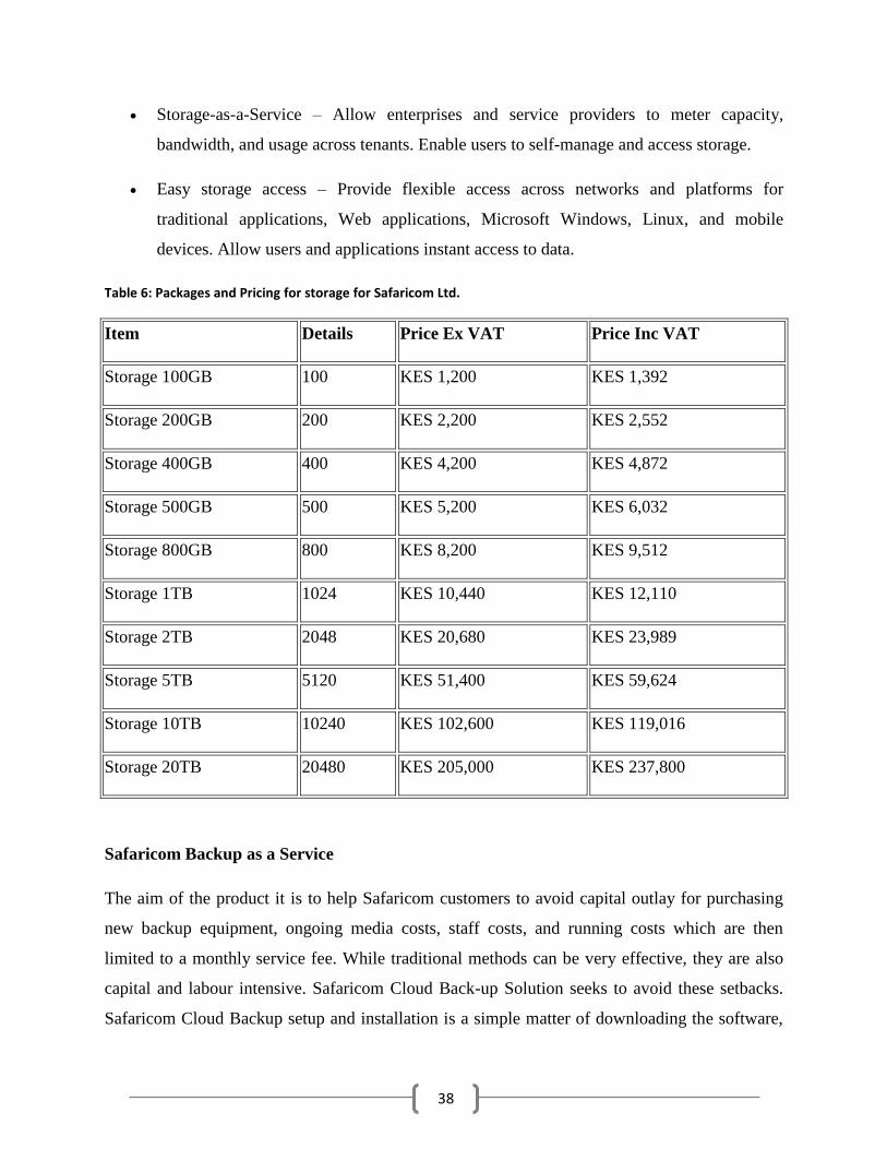
Table 6: Packages and Pricing for storage for Safaricom Ltd.
Item Details Price Ex VAT Price Inc VAT
Storage 100GB 100 KES 1,200 KES 1,392
Storage 200GB 200 KES 2,200 KES 2,552
Storage 400GB 400 KES 4,200 KES 4,872
Storage 500GB 500 KES 5,200 KES 6,032
Storage 800GB 800 KES 8,200 KES 9,512
Storage 1TB 1024 KES 10,440 KES 12,110
Storage 2TB 2048 KES 20,680 KES 23,989
Storage 5TB 5120 KES 51,400 KES 59,624
Storage 10TB 10240 KES 102,600 KES 119,016
Storage 20TB 20480 KES 205,000 KES 237,800
Safaricom Backup as a Service
The aim of the product it is to help Safaricom customers to avoid capital outlay for purchasing
new backup equipment, ongoing media costs, staff costs, and running costs which are then
limited to a monthly service fee. While traditional methods can be very effective, they are also
capital and labour intensive. Safaricom Cloud Back-up Solution seeks to avoid these setbacks.
Safaricom Cloud Backup setup and installation is a simple matter of downloading the software,

39
and takes only a few minutes to set up. Data recovery is equally fast, as there is no searching for
the right tape or waiting for IT staff to recover lost data. Once the application has been installed,
data transfer will be performed via a secure Internet connection (SSL) from the client site to the
Safaricom data store where the backup will reside.
Service Offers
Disk-to-Disk data backup and recovery solution which is uniquely designed for network
efficiency
Centralized management.
Policy-based control and ease of use.
An effective and efficient platform for a totally automated and secure data backup and
recovery for servers, databases, desktops and laptop devices.
Eliminates risk of human error in the backup process.
2-Factor authentication to your secured data
Backup disk capacity – scalable on demand
Features
Faster backup and recovery - Data DE duplication significantly reduces backup windows
by only storing unique daily changes while maintaining daily full backups for immediate
single-step restore.
Secure, off-site protection and enterprise class data encryption.
Multiple agent deployment options include download, email and redistributable
packages.
Self-service recovery capabilities for employees.
Powerful data history.

40
Benefits
Flexible deployment - Avamar systems scale to 124 TB of DE duplicated capacity.
It keeps data protected while in transit and at rest while also allowing it to be restored to
any Internet-connected location.
It makes the service easy to deploy to individuals - whether in the office or out of office.
One-step recovery – every Avamar backup is a full backup, which makes it easy for you
to browse, point, and click for a single-step recovery.
Data is stored for the life of your contract unless it is deleted from your computer or
replaced by a newer version – it will then be removed from your backup after 90 days.
Table 7: Packaging and Pricing for cloud backup service for safaricom Ltd.
Item Details Price Ex VAT Price Inc VAT
Backup 20GB 20 KES 850 KES 986
Backup 40GB 40 KES 1,150 KES 1,334
Backup 50GB 50 KES 1,300 KES 1,508
Backup 100GB 100 KES 1,650 KES 1,914
Backup 200GB 200 KES 3,210 KES 3,724
Backup 400GB 400 KES 5,810 KES 6,740
Backup 500GB 500 KES 7,110 KES 8,248
Backup 800GB 800 KES 11,010 KES 12,772

41
Backup 1TB 1024 KES 13,922 KES 16,150
Backup 2TB 2048 KES 27,234 KES 31,591
Backup 5TB 5120 KES 67,170 KES 77,917
Backup 10TB 10240 KES 133,730 KES 155,127
Backup 15TB 15360 KES 200,290 KES 232,336
Backup 20TB 20480 KES 266,850 KES 309,546

42
2.3 Machine learning
2.3.1 Definition of machine learning?
Machine Learning is the study of computer algorithms that improve automatically through
experience. Applications range from data mining programs that discover general rules in large
data sets, to information filtering systems that automatically learn users' interests
(mitchell,1996) .
Machine Learning is concerned with the design and development of algorithms that allow
computers to evolve behaviors based on empirical data, such as from sensor data or databases. A
major focus of Machine Learning research is to automatically learn to recognize complex
patterns and make intelligent decisions based on data; the difficulty lies in the fact that the set of
all possible behaviors given all possible inputs is too complex to describe generally in
programming languages, so that in effect programs must automatically describe programs.
2.3.2 Applications of machine learning
In recent years many successful machine learning applications have been developed, ranging
from data-mining programs that learn to detect fraudulent credit card transactions, to
information-filtering systems that learn users' reading preferences, to autonomous vehicles that
learn to drive on public highways. At the same time, there have been important advances in the
theory and algorithms that form the foundations of this field.
The poor performance results produced by statistical estimation models have flooded the
estimation area for over the last decade. Their inability to handle categorical data, cope with
missing data points, spread of data points and most importantly lack of reasoning capabilities has
triggered an increase in the number of studies using non-traditional methods like machine
learning techniques (Yogesh Singh, et. al). The area of machine learning draws on concepts from
diverse fields such as statistics, artificial intelligence, philosophy, information theory, biology,
cognitive science, computational complexity and control theory.

43
2.3.3 Types of machine learning
There are two main types of Machine Learning algorithms. In this work, supervised learning is
adopted here to build models from raw data and perform regression and classification.
Supervised learning: Supervised Learning is a machine learning paradigm for acquiring
the input-output relationship information of a system based on a given set of paired input-
output training samples. As the output is regarded as the label of the input data or the
supervision, an input-output training sample is also called labeled training data, or
supervised data. Learning from Labeled Data, or Inductive Machine Learning (Kotsiantis,
2007). The goal of supervised learning is to build an artificial system that can learn the
mapping between the input and the output, and can predict the output of the system given
new inputs. If the output takes a finite set of discrete values that indicate the class labels
of the input, the learned mapping leads to the classification of the input data. If the output
takes continuous values, it leads to a regression of the input. It deduces a function from
training data that maps inputs to the expected outcomes. The output of the function can
be a predicted continuous value (called regression), or a predicted class label from a
discrete set for the input object (called classification). The goal of the supervised learner
is to predict the value of the function for any valid input object from a number of training
examples. The most widely used classifiers are the Neural Network (Multilayer
perceptron), Support Vector Machines, k-nearest neighbor algorithm, Regression
Analysis, Artificial neural networks and time series analysis.
Unsupervised learning: Unsupervised learning studies how systems can learn to represent
particular input patterns in a way that reflects the statistical structure of the overall
collection of input patterns. By contrast with supervised learning or reinforcement
learning, there are no explicit target outputs or environmental evaluations associated with
each input; rather the unsupervised learner brings to bear prior biases as to what aspects
of the structure of the input should be captured in the output.

44
2.3.4 Techniques for supervised machine learning
In this section the researcher describes machine learning techniques, the ones that will be most
relevant to our work.
Linear Regression (LR) algorithm:
The goal of linear regression is to adjust the values of slope and intercept to find the line that best
predicts Y from X. More precisely, the goal of regression is to minimize the sum of the squares
of the vertical distances of the points from the line. When one thinks of regression , they think
prediction. A regression uses the historical relationship between an independent and a dependent
variable to predict the future values of the dependent variable. Businesses use regression to
predict such things as future sales, stock prices, currency exchange rates, and productivity gains
resulting from a training program. A regression models the past relationship between variables to
predict their future behavior. To make better models, we minimize the errors .an error is
considered to be the distance between the actual data and the model data. A Regression Line is
drawn so that there is minimal amount of error in predictions for all of the already known values
Equation of a Regression Line
The equation of a straight line shown below may be viewed as one of the equations of a
regression line
F(x)=mx+b
Variables, constants, and coefficients are represented in the equation of a line as
- x represents the independent variable
- f (x) represents the dependent variable
-the constant b denotes the y-intercept and this will be the value of the dependent variable if the
independent variable is equal to zero
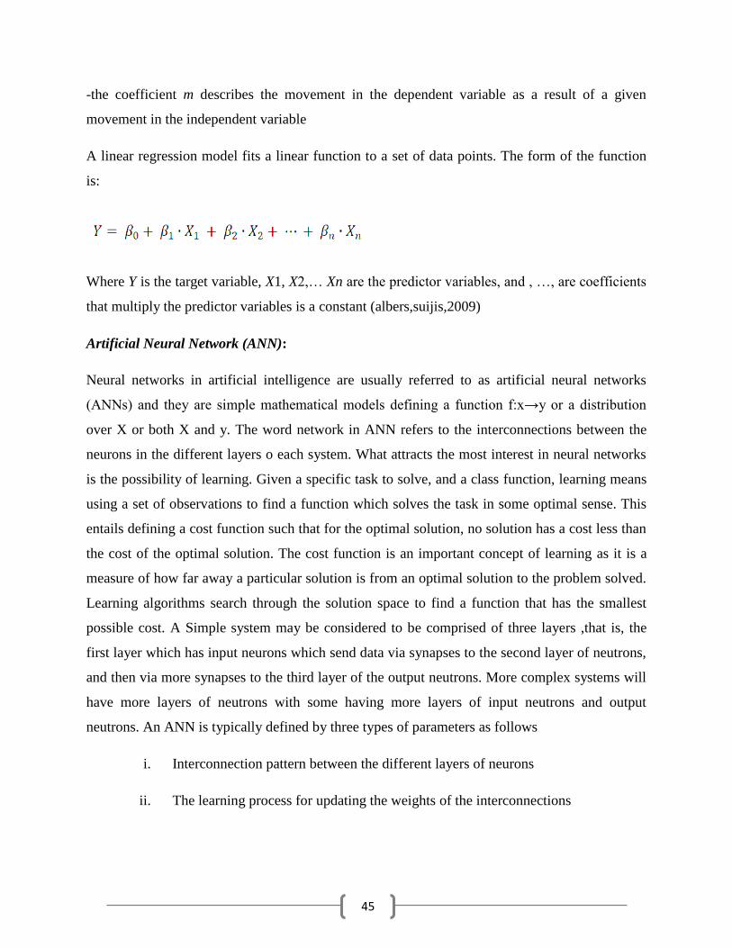
45
-the coefficient m describes the movement in the dependent variable as a result of a given
movement in the independent variable
A linear regression model fits a linear function to a set of data points. The form of the function
is:
Where Y is the target variable, X1, X2,… Xn are the predictor variables, and , …, are coefficients
that multiply the predictor variables is a constant (albers,suijis,2009)
Artificial Neural Network (ANN):
Neural networks in artificial intelligence are usually referred to as artificial neural networks
(ANNs) and they are simple mathematical models defining a function f:x→y or a distribution
over X or both X and y. The word network in ANN refers to the interconnections between the
neurons in the different layers o each system. What attracts the most interest in neural networks
is the possibility of learning. Given a specific task to solve, and a class function, learning means
using a set of observations to find a function which solves the task in some optimal sense. This
entails defining a cost function such that for the optimal solution, no solution has a cost less than
the cost of the optimal solution. The cost function is an important concept of learning as it is a
measure of how far away a particular solution is from an optimal solution to the problem solved.
Learning algorithms search through the solution space to find a function that has the smallest
possible cost. A Simple system may be considered to be comprised of three layers ,that is, the
first layer which has input neurons which send data via synapses to the second layer of neutrons,
and then via more synapses to the third layer of the output neutrons. More complex systems will
have more layers of neutrons with some having more layers of input neutrons and output
neutrons. An ANN is typically defined by three types of parameters as follows
i. Interconnection pattern between the different layers of neurons
ii. The learning process for updating the weights of the interconnections

46
iii. The activation function that converts a neuron’s weighted input to its output
activation
Training a neural network model essentially means selecting one model from the set of allowed
models that minimizes the cost criterion. Most of the algorithms used in training artificial neural
networks employ some form of gradient descent. This is done y simply taking the derivative of
the cost function with respect to network parameters and then changing these parameters in a
gradient-related direction.
It is defined by an interconnected group of functions that emulates a biological neural system and
can collectively perform complex tasks. During the training phase, an ANN changes its structure
based on external or internal information that flows through the network. Radial Basis Function
network (RBFn) is a feed forward ANN, typically with three layers: input, hidden and output. A
variable number of neurons form the key hidden layer, where Euclidean distance from the center
of each neuron to the test case is computed and the RBF function applied. RBFn is very similar
to k-nn, except for the fact that RBFn is a parametric method. The number of neurons in the
hidden layer (number of neighbors in k-nn) affects the performance and the computational
demands of RBFn. In the extreme case (over fitting), each data point can be the center of a
neuron (single neighbor in k-nn). The use of RBFn combined with a Bayesian network was
proposed for eliminating attributes with low correlation with the outcome (Duan&nadem, 2009).

47
Input Layer
A vector of predictor variable values (x1…xp) is presented to the input layer. The input layer (or
processing before the input layer) standardizes these values so that the range of each variable is -
1 to 1. The input layer distributes the values to each of the neurons in the hidden layer. In
addition to the predictor variables, there is a constant input of 1.0, called the bias that is fed to
each of the hidden layers; the bias is multiplied by a weight and added to the sum going into the
neuron.
Hidden Layer
Arriving at a neuron in the hidden layer, the value from each input neuron is multiplied by a
weight (wji), and the resulting weighted values are added together producing a combined value
uj. The weighted sum (uj) is fed into a transfer function, σ, which outputs a value hj. The outputs
from the hidden layer are distributed to the output layer.
Output Layer
Arriving at a neuron in the output layer, the value from each hidden layer neuron is multiplied by
a weight (wkj), and the resulting weighted values are added together producing a combined value
vj. The weighted sum (vj) is fed into a transfer function, σ, which outputs a value yk. The y
values are the outputs of the network.
If a regression analysis is being performed with a continuous target variable, then there is a
single neuron in the output layer, and it generates a single y value. For classification problems
with categorical target variables, there are N neurons in the output layer producing N values, one
for each of the N categories of the target variable.
The goal of the training process is to find the set of weight values that will cause the output from
the neural network to match the actual target values as closely as possible. There are several
issues involved in designing and training a multilayer perceptron network:
i. Selecting how many hidden layers to use in the network.
ii. Deciding how many neurons to use in each hidden layer.
iii. Finding a globally optimal solution that avoids local minima.
iv. Converging to an optimal solution in a reasonable period of time.
v. Validating the neural network to test for over fitting.

48
Support Vector Machine (SVM) algorithm:
It is a kernel method for solving classification problems (vapnik, et.al) and regression problems
especially for scenarios with non-linear learning pattern. The attribute space is transformed by
the kernel function into possibly a high-dimension feature space where an optimal linear
hyperplane is found by maximizing the margin between the so called support vectors. The
advantages of this method include the limited number of parameters to choose, and the ability to
handle large numbers of attributes and non-linear scenarios without local minima problems. A
comparison of radial basis function neural networks with SVM has been presented with lower
errors for SVM in some scenarios at the cost of higher computational demand.
Time series analysis:
Time series analysis is the process of using statistical techniques to model and explain a time-
dependent series of data points. Time series forecasting is the process of using a model to
generate predictions or forecasts for future events based on known past events. Time series data
has a natural temporal ordering and this differs from typical data mining/machine learning
applications where each data point is an independent example of the concept to be learned, and
the ordering of data points within a data set does not matter. Time series are analyzed in order to
understand the underlying structure and function that produce the observations. Understanding
the mechanisms of a time series allows a mathematical model to be developed that explains the
data in such a way that prediction, monitoring, or control can occur.
It is assumed that a time series data set has at least one systematic pattern. The most common
patterns are trends and seasonality. Trends are generally linear or quadratic. To find trends,
moving averages or regression analysis is often used. Seasonality is a trend that repeats itself
systematically over time. A second assumption is that the data exhibits enough of a random
process so that it is hard to identify the systematic patterns within the data. Time series analysis
techniques often employ some type of filter to the data in order to dampen the error. Other
potential patterns have to do with lingering effects of earlier observations or earlier random
errors.

49
General model of time series
Let an observed discrete time series be s1, . . . , sT . This means that we have T numbers which
are observations on some variable made at T equally distant time points, which we may label 1,
2, . . . , T.A fairly general model for the time series can be written
st = g(t) + ϕt where t = 1, . . . , T
The observed series is made of two components
Systematic part: g(t), also called signal or trend, which is a deterministic function of time
Stochastic sequence: a residual term ϕt, also called noise, which follows a probability law.
(Mitchell, 1996)
2.3.5 Application of supervised machine learning techniques in resource management
Machine learning theory presents various theoretical ideas on improving learning while the
practical aspect involves construction and improvements of algorithms for implementing the
learning. There is much literature available on machine learning and their areas of applications.
The use of Machine learning algorithms to predict application resource consumption is an
appealing approach that has been pursued by several previous studies (matsunaga& fortes, 2010).
The prediction of resources such as amounts of CPU, memory, disk and network required by an
application and the length of time which the resources are occupied can be viewed as a
supervised machine learning problem (matsunaga& fortes,2010).The system needs to learn a
concept based on a collection of historical data of n previous runs of the application. Each
previous observation is observed as training data. Examples of machine learning algorithms used
in learning and prediction of resource usage and consumption include linear regression
algorithm(LR),Artificial neural networks (ANN),support vector machines(SVM),and Time series
methods (matsunaga& fortes,2010).
Profile-Driven Storage provides visibility into an organization’s storage pool, letting it optimize
and automate storage provisioning. It gives administrators the ability to overcome upfront
storage provisioning challenges, such as capacity planning, differentiated service levels and

50
managing capacity headroom. Administrators can meet growing business needs by provisioning
data stores at scale, eliminating the need to provision virtual machines on a case-by-case basis.
Manage initial and ongoing virtual machine placement based on pre-defined
requirements.
Create data store clusters to support Storage DRS.
Gain deep insight into storage characteristics via integration with vSphere APIs for
Storage Awareness (VASA).
Dynamic Storage Provisioning
Using Profile-Driven Storage, various storage characteristics, including SLA, availability and
performance, can be requested in a virtual machine storage profile. These profiles are used to
ensure that only those data stores or data store clusters that are compliant with the virtual
machine storage profile are made available. The virtual machine storage profile can also help
select a similar type of data store when creating a Storage DRS data store cluster. Profile-Driven
Storage will reduce manual administration for virtual machine placement while improving
virtual machine SLA storage compliance
(http://www.vmware.com/products/vsphere/features/profile-driven-storage.html)
Accurate modeling of an application’s performance is very useful both for users and cloud
service providers. However, the non-linear relationship of resource allocations to application
performance, the interplay of resource usage across different types of resources, and resource
contention in a virtualized environment makes it very difficult to create application performance
models. The researchers identified three VM resource control parameters as sufficient inputs for
creating performance models. They also evaluated the effectiveness of artificial neural network
(ANN) and Support Vector Machine (SVM) techniques for modeling and demonstrated that
these are superior to conventional regression-based approaches. In order to further increase the
accuracy of these techniques, the researcher presented a sub-modeling technique that
substantially reduced prediction errors across five virtualized benchmark workloads from the

51
RUBiS and Filebench suites. Median and 90th
percentile prediction errors using ANNs were
reduced from 7.14% and 101.68% respectively (averaged across the workloads) for a correctly
configured single global model to 4.36% and 29.17% with sub-modeling. Finally, when the
models were used in VM sizing experiments, they delivered optimal results for 65% of the sizing
problems we studied and produced sizes that were close to optimal for the remaining 35%. They
expect that cloud users and service providers can benefit from the ability to create accurate
performance models for their virtualized workloads and utilize such models for accurate VM
sizing and placement (sajib kundu et. al).
Another study on the use machine learning techniques to map out resource consumption was
done by adrea matsunanga and jose fortes.The researcher reported in the paper considered the
problem of accurately predicting application resource usage, reviewed and discussed several
noteworthy machine learning algorithms considered by previous work, proposed and
implemented PQR2, an extension of an existing classification tree algorithm, and compared all
solutions (including the new PQR2 algorithm) under several conditions. Experiments predicting
execution time, memory and disk requirements for two popular bioinformatics applications,
BLAST and RAxML, were performed on a heterogeneous environment. Overall, PQR2
exhibited better accuracy when compared to other algorithms, due to its ability to better adapt to
scenarios with different characteristics (linear and non-linear relationships, high and low
density of training data points) by choosing different models for its nodes and leaves. At a more
general level, the two main conclusions from the work reported in this paper are as follows:
The scenarios requiring application resource prediction present a diverse behavior, making
different algorithms perform better in different situations. The use of methods that can adapt to
these situations by considering different configurations and algorithms is key for improving the
quality of the prediction without requiring manual tuning. The resulting algorithms may be
computationally more demanding during training, but this is usually not a concern as there is no
need to generate a new model very often. Roughly, using the largest dataset (BLAST), PQR2
required a few minutes to create the model and a few milliseconds to produce a single
prediction, indicating practicality of PQR2 for production deployments. PQR2 proved to be the
best solution for BLAST and RAxML and should be considered as candidate solution for other
applications.

52
Attributes can have high impact on the performance of the learning algorithms. The use of
system performance attributes showed to be relevant for execution time prediction whereas
application specific attributes were pertinent for all scenarios. This work makes the case for
including as many attributes as available, while letting the algorithms analyze the relevance of
the attributes when necessary. For cloud and grid computing scenarios, where resources are
outsourced, the provision of this information to its users (or services acting on behalf of the
users) through the use of benchmarks and runtime monitoring, especially of shared resources,
can bring several benefits. Although this information is not readily available on a per application
run basis, especially for shared resources, we expect it to become available in the near future
(Amazon CloudWatch is one such example limited to a virtual machine instance). Improved
prediction can result in better system utilization can avoid application abortion in system that
enforce accurate resource reservation, as well as significant savings when choosing the
appropriate pay- as-you-go resource (matsunaga& fortes,2010).
2.3.6 Tools used in machine learning and predictive modeling
Machine learning tools are utilities which can be used to analyze statistical datasets to
automatically learn users' interests. One of the most useful applications of statistical analysis is
the development of a model to represent and explain the relationship between data items
(variables).These tools comprise of a collection of various algorithms that are useful in machine
learning, and they allow users to capture datasets then they analyze these datasets for
relationships based on these algorithms. These machine learning tools also have a graphical
output representation utility which displays the results of the learning in the form of graphical
charts and tables. Some of these tools include:
Sysweka model
Machine Learning techniques based on Weka are adopted to build a middleware platform called
―SysWeka‖. Weka (Waikato Environment for Knowledge Analysis) is a popular suite of
machine learning software written in Java, developed at the University of Waikato, New
Zealand.Sysweka extends Weka capabilities and provide a software interface for usage by higher

53
application for managing resources on cloud systems(Alonso et.al).Weka supports several
standard data mining tasks, more specifically, data preprocessing, clustering, classification,
regression, visualization, and feature selection. All of Weka's techniques are predicated on the
assumption that the data is available as a single flat file or relation, where each data point is
described by a fixed number of attributes (normally, numeric or nominal attributes, but some
other attribute types are also supported). Weka provides access to SQL databases using Java
Database Connectivity and can process the result returned by a database query. It is not capable
of multi-relational data mining, but there is separate software for converting a collection of
linked database tables into a single table that is suitable for processing using Weka. Another
important area that is currently not covered by the algorithms included in the Weka distribution
is sequence modeling (Ian H. Wittenet. al, 2011).
DTREG
DTREG is one of the most useful applications of statistical analysis in the development of a
model to represent and explain the relationship between data items (variables). Many types of
models have been developed, including linear and nonlinear regression (function fitting),
discriminant analysis, logistic regression, support vector machines, neural networks and decision
trees (Phillip H. Sherrod, 2009).
Each method has its advantages. There is no single modeling method that is best for all
applications. DTREG provides the best, state-of-the-art modeling methods including neural
networks, decision trees, TreeBoost, decision tree forests, support vector machines (SVM), gene
expression programming, K-Means clustering, discriminant analysis and logistic regression. By
applying the right method to the problem, the analyst using DTREG should be able to match or
exceed the predictive ability of any other modeling program DTREG is a Predictive Modeling
Software that builds classification and regression decision trees, neural networks, support vector
machine (SVM), GMDH polynomial networks, gene expression programs, K-Means clustering,
discriminant analysis and logistic regression models that describe data relationships and can be
used to predict values for future observations.

54
DTREG accepts a dataset containing of number of rows with a column for each variable. One of
the variables is the ―target variable‖ whose value is to be modeled and predicted as a function of
the ―predictor variables‖. The tabular dataset in the form of rows and columns is the only format
that DTREG accepts data in.
DTREG analyzes the data and generates a model showing how best to predict the values of the
target variable based on values of the predictor variables using a number of tests for accuracy
from the various predictions. DTREG can create classical, single-tree models and also TreeBoost
and Decision Tree Forest models consisting of ensembles of many trees. DTREG also can
generate Neural Networks, Support Vector Machine (SVM), Gene Expression
Programming/Symbolic Regression, K-Means clustering, GMDH polynomial networks, and
Discriminate Analysis, Linear Regression, and Logistic Regression models.
Rapid miner
RapidMiner is a software platform developed by the company of the same name that provides
an integrated environment for machine learning, data mining, text mining, predictive analytics
and business analytics. It is used for business and industrial applications as well as for research,
education, training, rapid prototyping, and application development and supports all steps of the
data mining process including results visualization, validation and optimization This is an
environment for machine learning, data mining, text mining, predictive analytics, and business
analytics. It is used for research, education, training, rapid prototyping, application development,
and industrial applications. RapidMiner provides data mining and machine learning procedures
including: data loading and transformation (ETL), data preprocessing and visualization,
modeling, evaluation, and deployment (Rapidminer).
2.5 summary of literature review
As per the literature study, the researcher was able to review cloud platforms and the various
machine learning approaches under supervised learning and how they could be used to predict
resource consumption. More research was evidently needed on issues relating to learning
customer usage patterns for the case of storage resources most of them being statistical
techniques as suggested by literature reviewed concerning the IaaS cloud computing providers

55
and more specifically Safaricom limited. Various tools also exist for the management of the
cloud computing IaaS storage resources and each one of them is applicable for some specific
user needs.
2.6 Conceptual model
Figure 2-Process for using a machine learning technique to predict client storage resource usage.
PREDICTION
SOFTWARE
(DTREG)
MANUAL
CLASSIFICATION
RECORD OF
PERFORMANCE OF
THE TECHNIQUES
COMPARISON OF ACTUAL
VS PREDICTED RESULTS
TRAINED SET
PREDICTED
RESULTS
TRAINING SET
VALIDATION
MODEL
RAW DATA

56
CHAPTER THREE : METHODOLOGY
3.0 Introduction
Research methodology is a way to systematically solve the research problem. It may be
understood as a science of studying how research is done scientifically. In it we study the various
steps that are generally adopted by a researcher in studying his research problem along with the
logic behind them. It is necessary for the researcher to know not only the research
methods/techniques but also the methodology (Kothari, 2004).The objective of the research was
to carry out a comparative study of three machine learning techniques to identify which one
could best be used for learning of storage resource usage patterns for cloud clients and giving
predictions of future resource usage patterns. In this case, the researcher focused on supervised
learning because, from the data collected which could be used as training data for the learning
and prediction through the use of the machine learning techniques.
3.1 Research design
3.1.1 Introduction
This is a detailed outline of how the research was designed. A research design will typically
include selection and operationalisation of variables, selection of the type of study, selection of
data collection instruments, selection of the research sampling technique and data analysis the
intended means for analyzing data collected.
3.1.2 Selection of variables/Type of data required
Dependent variable: A dependent variable is one whose values are to be modeled and predicted
by other variables. The dependent variables or target variables in this study were usage of the
storage resource on a monthly basis, and the total amount of resource consumed after six months.
Independent variables: An independent variable also known as predictor variable is one whose
value will be used to predict the value of the dependent or target variables.
The independent variables in this study are the client requests for resources, and number of users
in the organization while the dependent variable was the resource usage after a period of six

57
months, number of users in the organization and the type of cloud IaaS storage service the client
is offered.
3.1.3 Type of study
In this case the researcher used the research approach is experimental research. The experimental
research design has the following generals steps.
i. Identify and define the problem
ii. Formulate hypothesis and deduce its consequences
iii. Construct an experiment that represents all the elements conditions and relations
iv. Conduct experiments
v. Compile the raw data and analyze it
vi. Conclusion
The research methodology used was experimental research which involved the use of the
framework for ensemble learning (ELF) (Hsuan-Tien lin, ling li, 2008) .It is a stand-alone
supervised machine learning framework. ELF is able to solve regression as well as classification
problems. The optimization target can be the RMSE, MAE, AUC or the classification error. The
ELF supports multi-class classification problems and multi-domain classification. Multi-domain
means that we have more than one label per example. The ELF has well implemented base
learners. The ensemble functionality of the framework is realized with stacking, cascade learning
and residual training. Stacking is a simple linear combination. ELF has the opportunity of
cascade learning, which is an extension of the features with predictions from other models.
Parameter selection can be done with cross-validation or bagging. Parameter selection means
searching for good meta-parameters in order to control over fitting of each individual model.
i. Data collection
ii. Analysis and preparation of data
iii. Run data through machine learning tool
iv. Test various prediction models using machine learning tools
58
v. Repeat prediction accuracy experiments with various models
vi. Analysis of results
3.1.5 Data Collection of training data
3.1.5.1 Data collection instruments
The data was collected through the use of questionnaires which were presented to the Safaricom
systems engineers. A sample of this has been attached in the appendix section (appendix 3) of
this document. Also through secondary sources which includes document review for the client
request
3.1.5.2 Research Sample design
3.1.5.2.1 Research population
The resource consumption data was collected from Safaricom limited while 70 % of the data was
simulated using curve fitting. Safaricom live data about how clients are using the requested
storage resource was collected for the purpose of the research study. This included data about
storage resource allocation, resource utilization, and the client request for these resources. The
data was on nature of organization (size and magnitude), resource requests storage, and resource
usage for storage. This data was for corporate organizations.
The data collected to be collected was for the cloud storage resource requests and usage for the
clients of Safaricom ltd. These were the two most relevant data items as pertains to the research
experiments that were to be done. The data was collected through face to face interviews with
the Safaricom engineers responsible for cloud computing services at Safaricom. The data
collected was for duration of six months. This was the period from January 2013 up to and
including June 2013.The data included those requests ranging between 1000 gigabytes to 10000
gigabytes. The rest of the data to be used for the experiments would be simulated.
Simulation of additional dataset
Out of the two hundred records in our dataset that were used for the research, 30 data elements
were live data from Safaricom while the other 170 was generated through simulation. This data

59
has been attached in the appendix section on sample data experimented on, of this document
where the first thirty records represent the live data collected while the remaining one seventy
records were simulated. The justification for the simulation is because, for the learning algorithm
work sufficiently, it requires more training data set where 200 records would prove sufficient.
Curve fitting software (statfit)
The statfit software was used to simulate part of the data that was used for the study. It works by
identifying the curve of best fit for the data and that we can use this curve to generate more data.
Through the use of the tool statfit, the live data which was collected from Safaricom was fed
into the statfit software and through tests for goodness of fit, the software was able to curve fit
the data into a lognormal type of distribution and output for us the various parameters of this
distribution including the minimum value, the mean of included normal and the standard
deviation of included normal which are key parameters when using lognormal distributions. For
the case of the data that the researcher used, the equations generated by the tool for resource
requests was lognormal in nature and it had the following parameters lognormal (1000, 8.1,
0.619) and the equation for resource usage was also lognormal and it had the following
parameters lognormal (0,7.01,0.738).We could then use this parameters to generate more data
using the ―generate‖ option within the statfit tool. The researcher varied the parameters of the
lognormal equation including the minimum value of data which could be requested so as to
generate more values since the simulation tool could only generate data in batches of fifty
elements. A total of 250 data elements were used where 30 were live data collected from
Safaricom while 220 were the simulated data items A sample of this dataset can be found in the
appendix of this document.

60
3.1.7 Preparation of the data for training
Classification of data
Once the data was collected, it was then classified based on magnitude of client requests for the
cloud computing storage service on a six month cumulative basis measured in gigabytes. The
reason for the classification was to group the various clients’ requests so as to identify those
whose requests are above 1000 GB. The classification index for both the dependent and
independent variables is given by the table below.
Classification index
Table 8-classification of client requests for storage on a six month cumulative basis
LABEL INDEX
VERY HIGH 5
HIGH 4
MEDIUM 3
LOW 2
VERY LOW 1
Table 9-classification of cloud storage service request in Gigabytes
CLOUD SERVICE REQUESTS in Gbs(cr) CLASSIFICATION
1000-2000 1
2001-4000 2
4001-6000 3
6001-8000 4
ABOVE 8000 5

61
Training Data
The training data was comprised of 200 data elements and it was presented in Microsoft excel’s
.csv format. It was made up of parameters which included, the amount of storage requested,
amount of storage used and the number of users within a particular organization. This was the
data which was used for experimentation
3.1.7 Prediction accuracy experiments
Experiments were done on the data which was to represent cloud client service requests and the
actual usage of these services requested. This data was run on the DTREG software and two
main files were generated that is, training data and validation data. The two files had several
rows representing the various clients and two columns, one for requested resource and the other
for actual usage.
Two sets of data were used in the study. Training data set used for the analysis and the validation
data set used for validation. The training dataset has been attached in the appendix section while
the validation dataset is generated by the learning tool DTREG.
3.1.7.1 Experimental testbed for Prediction accuracy
The experiment was done using software called DTREG that would take in .csv files
representing the training set and the testing data, train the classifier using the training files and
then use the test file to perform the classification task on the test data. DTREG would then make
modifications to the data according to the model chosen and then when the analysis is run, it
produces results.
The experiments were performed using the following software’s:
Simulation software
The simulation software used was DTREG version 10.7.8
Operating system
The experiments were done on Microsoft windows 7 service operating system.

62
Spreadsheets (MS excel)
Microsoft was used for data analysis and result analysis to generate the bar graphs and line
graphs.
The training experiments to be carried out using DTREG. DTREG includes a full Data
Transformation Language (DTL) for transforming variables, creating new variables and selecting
which rows to analyze.
3.1.7.2 Prediction procedure
How to run data through DTREG: DTREG prediction software was given the data set for the
cloud computing service requests and it divided the data into the two data sets. The following are
fundamental steps that were undertaken
i. Load training file
ii. Load prediction file
iii. Assign class (predicted attribute)
iv. Select a prediction tool
v. Perform classifications training /testing using training/testing files
vi. Evaluate classification using cross validation method
vii. Perform predictions using prediction file
viii. Save predictions output as predictions file
Experiment design
The classified data, which is, resource request and utilization data was then subjected to
experimentation. The experiments were the test for accuracy done using the following measures:
Root mean square error, mean absolute percentage error and mean square error .They included
subjecting the training data to the DTREG tool getting the predictions and evaluating the
accuracy of prediction. The significance of this data is for training examples which will be run
on the machine learning tool (DTREG).From the data we can be able to survey for suggested
trends and patterns on the requests versus usage.

63
Machine learning methods were experimented upon in order to find the best predicting tool that
is accurate for the case of a cloud computing environment. The following machine learning
methods were used in the study: linear regression, Support Vector Machine (SVM) and artificial
neural networks (ANNs)
Various types of experiments were carried out and this included Test for accuracy in the actual
verses predicted results. Experiments were done on the data which was to represent cloud client
service requests and the actual usage of these services requested. This data was run on the
DTREG software and two main files were generated that is, training data and validation data.
The two files had several rows representing the various clients and two columns, one for
requested resource and the other for actual usage. The experiments for accuracy described earlier
were done using software called DTREG that would take in .csv files representing the training
set and the testing data train the classifier using the training files and then use the test file to
perform the classification task on the test data. DTREG would then make modifications to the
data according to the model chosen and then when the analysis is run, it produces results.
3.1.8 Data Analysis
3.1.8.1 Processing of prediction accuracy data
Tabulation of the prediction accuracy data collected
The data to be collected from the experiments included the prediction results from the various
machine learning techniques in the form of graphs and tables comparing the actual verses the
predicted results, the coefficient of variance between the actual verses the predicted results and
the various measures of accuracy for the various machine learning techniques including mean
absolute percentage error (MAPE), correlation between actual and predicted variables, mean
square error (MSE).
The experiments were done using DTREG software and the results tabulated and also presented
in form of graphs generated from Microsoft Excel.
The Actual data that was provided to the Model was compared with the predicted results
generated by the model using graphs.
64
3.1.8.1 Comparison of the Machine learning techniques
The machine learning algorithms were compared included Support vector machine algorithm
(SVM), linear regression and artificial neural networks (ANN).The experiments were run on
DTREG while changing the various parameters so as to see how the results differ. The
experiments involved a test for accuracy in the prediction of a machine learning algorithm. The
measures observed in the analysis included the coefficients of variance (CV) in the learning
algorithms, mean absolute percentage error (MAPE), correlation between actual and predicted
variables, mean square error (MSE).
As part of the experiments, the following metrics will be evaluated so as to measure the
algorithms’ performance. This metrics include mean absolute percentage error (MAPE),
Coefficient of Variation, root mean square error (RMSE), Correlation between actual and
predicted data

65
CHAPTER FOUR : RESULTS ANALYSIS AND EVALUATION
4.0 Introduction
This section describes the review and analysis of the results which were collected after
conducting the various comparisons of the machine learning algorithms using the DTREG tool.
It also contains the various results that were used to measure the accuracy of the various
algorithms used.
4.1 Data sets collected
The data set collected comprised of 30 records from Safaricom which were used to simulate
another 200 datasets as the training dataset. The training data was comprised of 200 data
elements and it was presented in Microsoft excel’s .csv format. It was made up of parameters
which included, the amount of storage requested, amount of storage used and the number of
users within a particular organization. This was the data which was used for experimentation.
4.1.1 Data set collected in tabular format
The data which was collected from Safaricom was used to generate some other data through
simulation and these datasets have been attached in the appendix section of this document

66
4.1.2 Graphical representation of data for Client resource(Storage) usage over six
months
Figure 3-Request verses usage over six months
This graph enables us to identify the trend that client usage for the requested resource is not
stagnant and it keeps on increasing steadily with time.
4.1.3 Resource requests verses the usage
This was done using Microsoft excel and the line graph below gives a representation of the
requests. The analysis from this is that the users tend to request for much more storage resource
than they actually use.
Res
ou
rce
usa
ge in
gig
abyt
es
Time (months)

67
Figure 4: Resource requested versus usage
4.2 Results of accuracy of prediction of resource usage
4.2.1 Tabular presentation
The results obtained from the Machine learning tool were printed out in the form of reports from
the software
Table 10-measures of accuracy for various learning model
4.2.2 Graphical presentation of results
4.2.2.1 Coefficient of variation
Client (ordered by number)
Sto
rage
re
sou
rce(
gbs)

68
Figure 5: Coefficient of variation
4.2.2.2 Root mean square error
Figure 6: Root mean square error
4.2.3.3 Mean absolute percentage error

69
Figure 7: Mean percentage error
4.2.2.4 Correlation between actual and predicted data
Figure 8: Correlation between actual and predicted values

70
4.3 Comparison of accuracy of the predictions by the various algorithms
The lower the Coefficient of Variation, the smaller the residuals relative to the predicted
value. This is suggestive of a good model fit. As from the analysis and this case ANN
has the best model fit followed by SVM since they exhibit the lower coefficients of
variation.
Two or more statistical models may be compared using their MSEs as a measure of how
well they explain a given set of observations: The unbiased model with the smallest MSE
is generally interpreted as best explaining the variability in the observations. From the
analysis of our experimental results and according to our dataset, ANN and SVM had the
smaller values hence they would be the preferred choice of algorithm.
When considering this metric the smaller the mean absolute percentage error (MAPE) the
better and from the analysis of our experimental results data SVM had theleast mean
percentage error.
From the graph, SVM had the most corellation between the actual and predicted
values.The higher the correllation the better for a prediction model.From the analysis of
the experimental results SVM would be the best machine learning technique judging by
the metric of correllation.
The researcher then usede the average of the above measures stated toevauate which will
be the best machine learning algorithm to use for this case of cloud storage resource
usage.All the three measures that is root mean square error,mean absolute deviation and
the correllation between actual and predicted data.
From the analysis of the results of experiments’ carried out by the researcher of the various
metrics mentioned earlier, that is, MAPE, RMSE, coefficient of variation and comparison
between actual verses predicted data, it is evident that support vector machine (SVM) is the best
machine learning approach for this particular case and it can be used as a tool for prediction of
client storage resource usage patterns for the case of cloud computing IaaS.
Support Vector Machines algorithm can therefore be used as a tool where the storage resource
usage patterns can be surveyed and then the trend that is observed be use to advice clients on
71
their future storage resource requirements. The observed usage patterns can also be used by
cloud computing providers when budgeting for their resource since they can be able to get the
projected clients storage resource requirements and therefore better future planning on their part
regarding the resources.
4.4 Limitations and challenges
The researcher acknowledges the challenge in compiling the actual usage data from the cloud
service provider .For this reason the researcher used estimates for the raw data and assumed that
the customer resource request and usage patterns remain fairly constant.
Due to time constraints, the researcher used only DTREG as his evaluation tool therefore the
researcher advices that other tools may be used to make the study more comprehensive.

72
CHAPTER FIVE : CONCLUSION AND RECOMMENDATIONS
5.1 Conclusion
In the study conducted for the purpose of this thesis, the main objective was to conduct a
comparative study of the machine learning techniques for optimizing the provision of storage
computing in cloud computing IaaS. In order to achieve this objective, forecasting of cloud client
requests was an important aspect towards achieving optimization since the cloud service
providers, in this particular case Safaricom, would be able to use this as planning information
when developing their storage infrastructure.
According to the experiments and supporting literature review, Support Vector Machine would
be the proffered machine learning algorithm used as per the results observed from the results of
the experiments of the research. It can be concluded therefore that through the use of support
vector machines(SVM), we can develop predictions that can be used as a basis for improving on
the efficiency of cloud service delivery and in turn optimization.
5.2 Recommendations
In this research, the researcher argues that the use of machine learning for the prediction of
storage resource usage for the case of cloud computing is an approach worth adopting and the
most accurate technique for this prediction would be support vector machine (SVM) learning
technique.
5.3 Further work
The predictions were based on one tool that is DTREG and it is advised that other prediction
tools be used such as WEKA, Hadoop and others .Further research is advised on developing
dynamic models which can adopt the usage of cloud resources based on the requests from the
users in real time. Also as an area for future research, the researcher suggests discussions and
research on how machine learning techniques can be used to improve other areas of cloud
computing that is PaaS and SaaS
Through the use of these predictions, clients can be appropriately advised and the cloud service
provider can also do provisions for the right amounts of the given storage resource.

73
REFFERENCES
1. A. Matsunaga and J. A. B. Fortes, ―On the use of machine learning to predict the time and
resources consumed by applications‖, in Proceedings of the 2010 10th IEEE/ACM International
Conference on Cluster, Cloud and Grid Computing, 2010, p. 495-504.
2.Antoine Bordes, Léon Bottou, Patrick Gallinari, and JasonWeston.Solving MultiClass Support
Vector Machines with LaRank In Zoubin Ghahramani, editor, Proceedings of the 24th
International Machine Learning Conference, pages 89–96, Corvallis,Oregon, 2007.
OmniPress.URL http://leon.bottou.org/papers/bordes-2007.
3. Arkaitz Ruiz-Alvarez, Marty Humphrey, A Model and Decision Procedure for Data Storage
in Cloud Computing, in Proceedings of the IEEE/ACM International Symposium on Cluster,
Ottawa Canada, 2012.
4. Corinna Cortes and Vladimir Vapnik. Support vector networks. In Machine Learning, pages
273–297, 1995.
5. Daniel Nurmi, Rich Wolski, Chris Grzegorczyk, GrazianoObertelli, Sunil Soman,
LamiaYouseff, DmitriiZagorodnov, (2009). “The Eucalyptus Open-source
CloudcomputingSystem”.In Proceedings of the IEEE/ACM International Symposium on Cluster
Computing and the Grid, 2009. IEEE Press.
6. Dustin Amrhein, Scott Quint. Cloud computing for the enterprise - Understanding cloud
computing and related technologies: Part 1: Capturing the cloud.
http://www.ibm.com/developerworks/websphere/techjournal/0904_amrhein/0904_amrhein.html,
2009.
7.Gihun Jung, Kwang Mong Sim, Location-Aware Dynamic Resource Allocation Model for
Cloud Computing Environment, in Proceedings of International Conference on Information and
Computer Applications, Dubai, 2011.

74
8. Hsuan-tien lin , Ling Li .”Support vector Machine for Infinite Ensemble learning”. Journal of
machine learning 9 (2008) pg 286-312
9. Ian H. Witten; Eibe Frank, Mark A. Hall (2011). "Data Mining: Practical machine learning
tools and techniques, 3rd Edition". Morgan Kaufmann, San Francisco. Retrieved 2011-01-19.
10. Kotsiantis S.B, Supervised Machine Learning: A Review of Classification Techniques.
Informatica31:249–268 (2007)
11. Kothari, Research methodology methods and techniques (2004)
12.L. Jiang, H. Zhang, Z. Cai and J. Su. Learning Tree Augmented Naive Bayes for Ranking.
Proceedings of the 10th International Conference on Database Systems for Advanced
Applications, 2005.
13. mahendra singh sagar,babita singh waseema ahmad. Study on cloud computing resource
allocation strategies .international journal of advanced research and innovation (AJARI)
VOLUME 3 (2013) ISSN 2347 - 3258
14. Mitchel, T. M. (1996). Machine Learning.McGraw Hill.
15. Navendu Jain, Ishai Menache, Ohad ShamirLearning-Based Resource Allocation for Delay-
Tolerant Batch Computing Microsoft Research
16. NIST definition of cloud computing,NIST special publication 800-145
17. Rahim, A. (n.d.). Machine Learning Using Support Vector Machines.Rajkamal Kaur Grewal,
Pushpendra Kumar Pateriya, A Rulebased Approach for Effective Resource Provisioning In
Hybrid Cloud Environment, IJCSI, VollIss4
18. Sajib kundu, raju rangaswani, ajay gulita , ming zao and kaushik dutta Modeling Virtualized
Applications using Machine Learning Techniques
19. Too emma chebet,a comparative study of machine Learning methods for
forecastingPrevalence of weather-based pests,2010

75
20. V.Vinothina, Dr.R.Sridaran, Padmavathi Ganapath A Survey on Resource Allocation
Strategies in Cloud Computing,(IJACSA) International Journal of Advanced Computer Science
and Applications ,Vol. 3, No.6, 2012
21. Yogesh Singh, Pradeep Kumar Bhatia & Omprakash SangwanA review of studies on
machine learning techniques International Journal of Computer Science and Security, Volume 1:
Issue (1)
22. Zhenyu Fang Resource management on Cloud systems with Machine Learning2010
23. http://www.cloudsigma.com/blog/40-cloud-resource-contention-bundling-issues-iaas
24. http://aws.amazon.com/
25. http://www.vmware.com/products/vsphere/features/profile-driven-storage.html
26.http://www.cloud-competence-center.com/understanding/cloud-computing-deployment-
models/
27.http://gigaom.com/2012/02/05/startup-takes-on-cloud-over-provisioning/
28. http://elf-project.sourceforge.net/

76
APPENDICES
Appendix 1:Screenshots for results
Comparative usage over six months

77
Actual versus predicted usage over six months

78
Appendix 2: Sample questions to Safaricom ltd. engineers
A) Are there optimization problems which Safaricom encounters with there cloud
computing infrastructure?
The main optimization problems would be in terms of computer resource utilization (CPU,
Memory and storage) usage.
There are defined limits that are set such a single customer should not use all/most of the
resources on the server to himself as this would choke out other users.
B) How are they solved?
Servers' status are constantly monitored and growth pattern graphed (the growth pattern is fairly
constant), so that either additional resources are added or new servers all together are deployed.
There are instances where the defined limits (web hosting) is too small for a customer, in such a
case the S/W allows for the Safaricom admin to increase the specific customers limit, though this
is done in very rare cases, as most likely the customer would be advised to optimize their
application to fit within the defined limits
C) Does Safaricom manage their own platform and if they do, what approach is used to
manage cloud resource?
We manage our own platforms on both IAAS and web hosting......(not sure how to answer the
approach question)
D) What Softwares are used to achieve the cloud management?
For IAAS we require to virtualize our environment, in this case we use VMware as our
hypervisor.

79
We use cpanel for our webhosting platform.
We also have monitoring solutions such as solar winds to monitor the servers and applications.
Appendix 3:Sample dataset experimented upon
RESOURCE
REQUESTED(gb)
total usage after 6
months(gb)
no. of
users
type of
service
1000 206.3 248 storage
2000 412.7 249 storage
3500 412.7 146 storage
1000 330.1 294 storage
10000 2475.9 107 storage
2000 907.8 227 storage
3000 1031.6 66 storage
5000 1650.6 260 storage
1000 247.6 264 storage
4000 1238 228 storage
5000 1650.6 152 storage
10000 3713.9 77 storage
3000 1238 186 storage
4500 1650.6 64 storage
4000 1238 127 storage
5000 1650.6 104 storage
3000 1031.6 202 storage
4000 1650.6 232 storage
10000 2475.9 120 storage
8000 1650.6 129 storage
3000 825.3 68 storage
4000 1444.3 157 storage
5000 2063.3 154 storage

80
8000 2888.6 88 storage
2500 1031.6 141 storage
3000 1031.6 50 storage
5000 825.3 117 storage
9000 2888.6 83 storage
1000 330.1 221 storage
4000 1568.1 227 storage
5000 1584.1 180 storage
10000 3755.6 388 storage
6500 2036.7 222 storage
3500 729.2 105 storage
3000 500.8 86 storage
4000 958.9 124 storage
3000 535.3 89 storage
4000 983.2 127 storage
10500 4021.7 415 storage
10000 3804.6 393 storage
4500 1082.8 135 storage
3000 572.3 92 storage
4500 1091.2 136 storage
4000 828.5 113 storage
4000 942.2 123 storage
3000 463.8 83 storage
4000 980.3 126 storage
3000 494.1 86 storage
8500 2937.1 307 storage
8000 2572.7 272 storage
4000 926.9 122 storage
6000 1732.4 193 storage
2000 211.3 64 storage
14000 5539.7 570 storage

81
3000 470.7 84 storage
5000 1340.5 158 storage
3500 645.4 98 storage
4500 1027.3 130 storage
3000 569.7 92 storage
6500 1935.8 212 storage
5000 1249.7 150 storage
4500 1166.8 143 storage
6500 2011.3 219 storage
4000 924.1 121 storage
6500 2011.4 219 storage
4000 918.3 121 storage
5000 1358.1 160 storage
6000 1746.3 195 storage
3000 489.3 85 storage
10000 3484.3 361 storage
5500 1562.7 178 storage
7000 2135.6 231 storage
6500 1865.3 206 storage
4500 1147.8 141 storage
5500 1494.1 172 storage
10000 3662.6 379 storage
3500 648.2 98 storage
5000 1294.5 154 storage
4000 954.8 124 storage
5000 1207.9 146 storage
10000 1594.1 264 storage
6500 3765.6 228 storage
3500 2046.7 152 storage
3000 739.2 77 storage
4000 510.8 186 storage

82
3000 968.9 64 storage
4000 545.3 127 storage
10500 993.2 104 storage
10000 4031.7 202 storage
4500 3814.6 232 storage
3000 1092.8 120 storage
4500 582.3 129 storage
4000 1101.2 68 storage
4000 838.5 157 storage
3000 952.2 154 storage
4000 473.8 88 storage
3000 990.3 141 storage
8500 504.1 50 storage
8000 2947.1 117 storage
4000 2582.7 83 storage
6000 936.9 221 storage
2000 1742.4 227 storage
14000 221.3 180 storage
8000 5549.7 388 storage
10000 480.7 222 storage
4500 1350.5 105 storage
3000 655.4 86 storage
4500 1037.3 124 storage
4000 579.7 89 storage
4000 1945.8 127 storage
3000 1259.7 415 storage
4000 1176.8 393 storage
3000 2021.3 135 storage
8500 934.1 92 storage
8000 2021.4 136 storage
4000 928.3 113 storage

83
6000 1368.1 123 storage
2000 1756.3 83 storage
14000 499.3 126 storage
3000 3494.3 86 storage
5000 1572.7 307 storage
3000 2145.6 272 storage
5000 1875.3 122 storage
1000 1157.8 193 storage
5000 1504.1 64 storage
4500 3672.6 570 storage
8000 658.2 84 storage
6500 1304.5 158 storage
5000 964.8 98 storage
6000 1217.9 130 storage
5000 1589.1 92 storage
4000 3760.6 212 storage
5000 2041.7 150 storage
6000 734.2 143 storage
3000 505.8 219 storage
10000 963.9 121 storage
5500 540.3 219 storage
7000 988.2 121 storage
6500 4026.7 160 storage
4500 3809.6 64 storage
5500 1087.8 570 storage
10000 577.3 84 storage
3500 1096.2 158 storage
1000 833.5 98 storage
4000 947.2 130 storage
5000 468.8 92 storage
10000 985.3 212 storage

84
6500 499.1 150 storage
3500 2942.1 143 storage
3000 2577.7 219 storage
4000 931.9 121 storage
3000 1737.4 219 storage
4000 216.3 121 storage
10500 5544.7 160 storage
10000 475.7 195 storage
4500 1345.5 85 storage
3000 650.4 361 storage
4500 1032.3 178 storage
5000 574.7 231 storage
8500 1940.8 206 storage
5000 1254.7 141 storage
6000 1171.8 172 storage
9000 2016.3 379 storage
4500 929.1 98 storage
8000 2016.4 154 storage
4000 923.3 124 storage
10500 1363.1 146 storage
6000 1751.3 264 storage
5000 494.3 228 storage
7000 3489.3 152 storage
3000 1567.7 77 storage
4500 2140.6 186 storage
6000 1870.3 64 storage
4000 1152.8 127 storage
6000 1499.1 104 storage
8000 3667.6 202 storage
5000 653.2 232 storage
6000 1299.5 143 storage

85
9000 959.8 219 storage
8000 1212.9 121 storage
6000 1604.1 219 storage
4000 3775.6 121 storage
10000 2056.7 160 storage
4000 749.2 64 storage
8000 520.8 570 storage
5000 978.9 84 storage
4000 555.3 158 storage
3000 1003.2 98 storage
4000 4041.7 130 storage
5500 3824.6 92 storage
7000 1102.8 212 storage
5000 592.3 150 storage
5000 1111.2 143 storage
6000 848.5 219 storage
5500 962.2 121 storage
4000 483.8 219 storage
8000 1000.3 121 storage
7500 514.1 160 storage
8000 2957.1 154 storage
5000 2592.7 124 storage
3000 946.9 146 storage
6000 1752.4 264 storage
4000 231.3 228 storage
10000 5559.7 152 storage
4000 490.7 77 storage
8000 1360.5 186 storage
5000 665.4 64 storage
4000 1047.3 127 storage
3000 589.7 104 storage
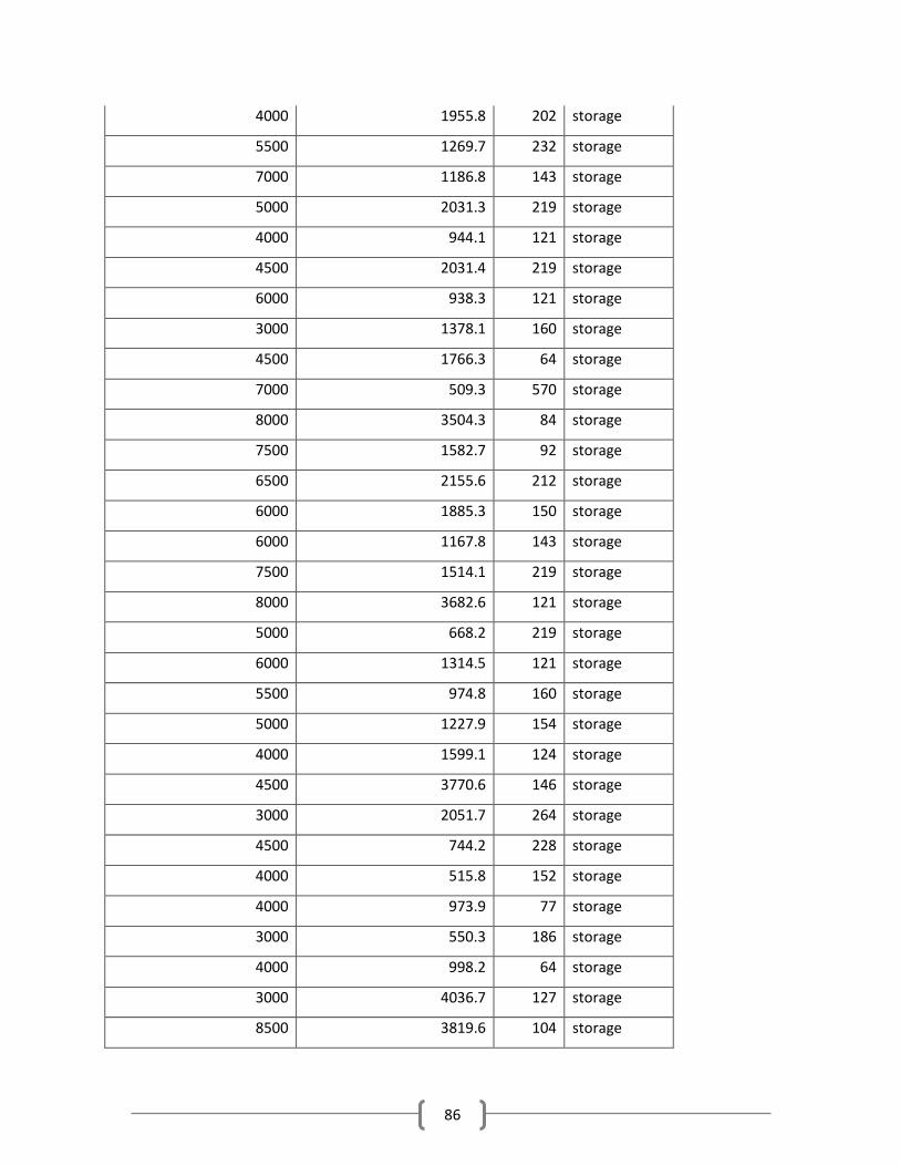
86
4000 1955.8 202 storage
5500 1269.7 232 storage
7000 1186.8 143 storage
5000 2031.3 219 storage
4000 944.1 121 storage
4500 2031.4 219 storage
6000 938.3 121 storage
3000 1378.1 160 storage
4500 1766.3 64 storage
7000 509.3 570 storage
8000 3504.3 84 storage
7500 1582.7 92 storage
6500 2155.6 212 storage
6000 1885.3 150 storage
6000 1167.8 143 storage
7500 1514.1 219 storage
8000 3682.6 121 storage
5000 668.2 219 storage
6000 1314.5 121 storage
5500 974.8 160 storage
5000 1227.9 154 storage
4000 1599.1 124 storage
4500 3770.6 146 storage
3000 2051.7 264 storage
4500 744.2 228 storage
4000 515.8 152 storage
4000 973.9 77 storage
3000 550.3 186 storage
4000 998.2 64 storage
3000 4036.7 127 storage
8500 3819.6 104 storage

87
8000 1097.8 202 storage
4000 587.3 232 storage
6000 1106.2 130 storage
2000 843.5 92 storage
14000 957.2 212 storage
3000 478.8 379 storage
5000 995.3 98 storage
8500 509.1 154 storage
6000 2952.1 124 storage
5000 2587.7 146 storage
Appendix 4:DTREG user manual screen shots
When you launch DTREG, its main screen displays:
Figure 9-DTREG-main screen
From this screen, you can

88
i. Create a new project to build a model by clicking
ii. Open an existing project by clicking
iii. Set options and enter your registration key.
Setting DTREG preferences
To set DTREG preferences, click ―Tools‖ on the menu bar and select ―Preferences‖ from the
dropdown menu.
Figure 10-DTREG screen for setting prefferences
Default type of model to build: Select which type of model you would like DTREG to create
for new projects (single tree, SVM neural network, etc.). You can always change the type of a
model later by modifying its properties.
Max. execution threads: Specify how many execution threads you want DTREG to use during
its computations. If you have a multi-CPU system, you can increase the speed of calculation by
allowing DTREG to use more than one CPU, but this will place a heavier load on your system.
Execution priority: Specify the preferred execution for DTREG to use during an analysis.
Currently the execution priority is only applied to neural network training processes.
Loading the training file

89
The first step in building a model the following are required:
Input data file –Specify the device, folder and name of the file containing the input (Learning)
dataset to be used to build the model. The data must be in a comma separated value (CSV) file
with the names of the variables on the first line.
Character used for a decimal point in the input data file – Select whether a period
or a comma will be used to indicate the decimal point in numeric values in the input
data file.
Character used to separate columns – Select the character that will be used to separate
columns in the input file. The default separator is a comma.
File where information about this project is to be stored – Specify the name of the
project files where DTREG will store parameters and computed values for the project. DTREG
project files are stored with the type ―.dtr.
Figure 11-DTREG screen for loading training data files and specifying storage location for outputs
The file loaded is the data used for training. The data is divided by the system into the two
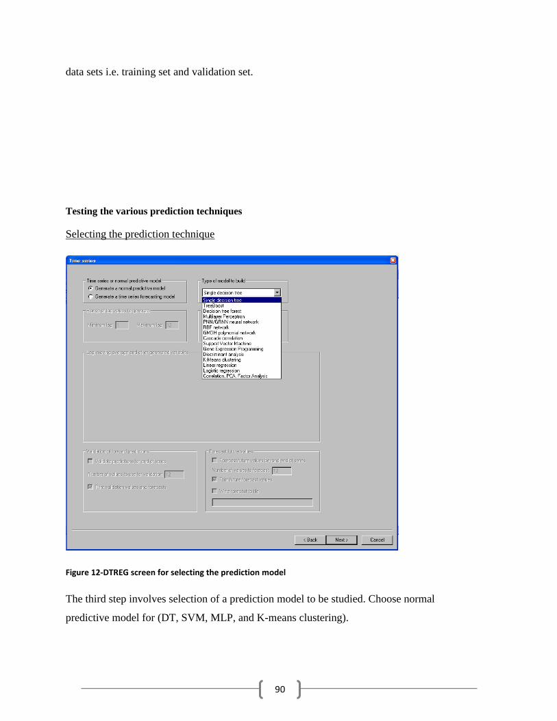
90
data sets i.e. training set and validation set.
Testing the various prediction techniques
Selecting the prediction technique
Figure 12-DTREG screen for selecting the prediction model
The third step involves selection of a prediction model to be studied. Choose normal
predictive model for (DT, SVM, MLP, and K-means clustering).
91
Assigning the classes
The fourth step involves selection of variables.
Classes of Variables
Specify the classes of variables to performing analyses:
Target variable: The target variable is the variable whose values are to be modeled and
predicted by other variables. It is analogous to the dependent variable. There must be one and
only one target variable. Our target variable is class index (resource usage) as shown on the table
below and should be categorically.
Predictor variable: A predictor variable is a variable whose values will be used to predict the
value of the target variable. It is analogous to the independent variables. There must be at least
one predictor variable specified, and there may be many predictor variables.
Our predictor variables were:
- Resource requested (RQ)
The predictor variables are continuous
Model testing and validation
Before running a model enabled the following settings that will be used to measure the
performance of the models:
Cross-validation Control Variable
This is used to evaluate the quality of a model it’s assigned a random set of rows to each
validation fold after stratifying on the target variable.

92
Figure 13-DTREG screen for setting model variables
Model validation record
Validation data row report file – If you enable this option and specify a file name in the edit
field, then DTREG will write a record to the file showing which rows were used for validation,
and it will show the predicted value for each validation row. Each row in the file has 4 columns:
(1) the data row number , (2) the actual value of the target variable, (3) the predicted value of the
target variable, and (4) an indication of correct/incorrect class residual value if doing regression
Run the model
Once you have done all the steps you can then tell DTREG to perform an analysis.
While an analysis is running, a progress screen will be displayed

93
Figure 14-DTREG screen for model creation
Results of analysis
When the model has completed its execution the results are displayed. There are several major
sections in the report.
The Project Parameters section of the report displays a summary of the options and parameters
selected for the model.
Figure 15-DTREG screen for results report

94
Input data section
The Input Data section displays information about the input data file used to construct the model.
The entry for ―Rows with missing target or weight values indicates the number of rows that
were discarded because these variables had missing values.
Summary of variables

95
Saving the prediction file
After completion of the analysis the project can then be saved for later referencing.

96