Machine Learning

Neural Networks (2)

Multi-layers Network

• Let the network of 3 layers

– Input layer

–Hidden layer

–Output layer

• Each layer has different number of neurons

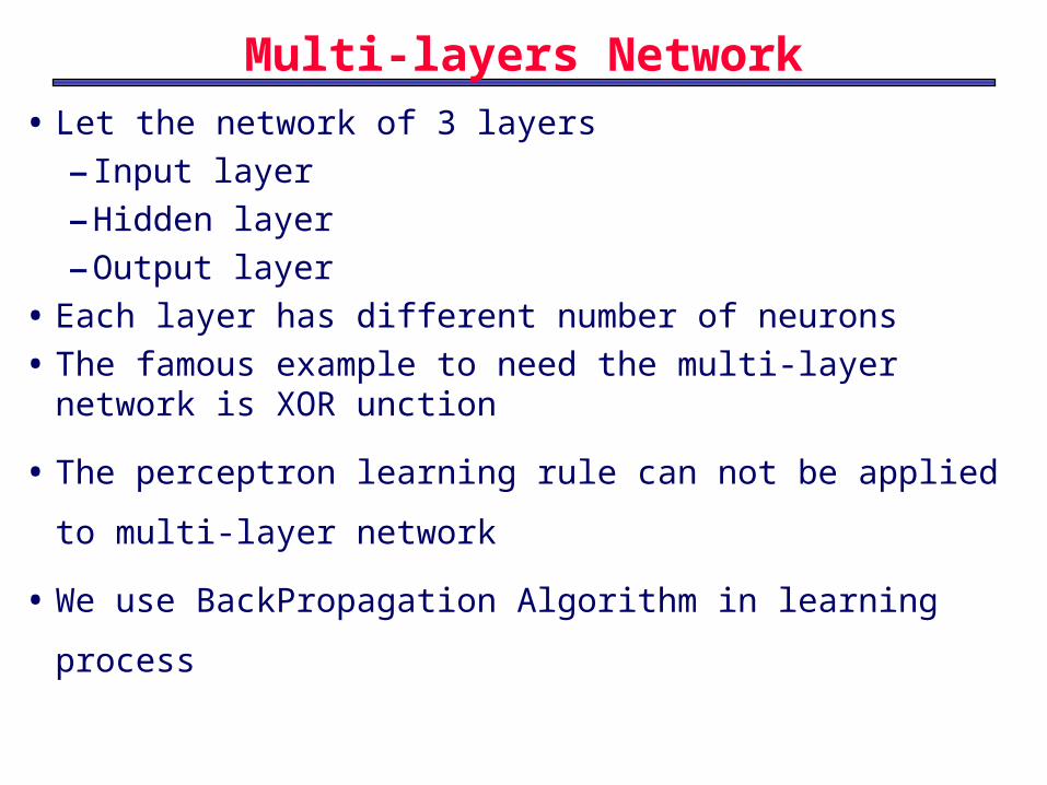
• The famous example to need the multi-layer network is XOR unction

• The perceptron learning rule can not be applied to multi-

layer network

• We use BackPropagation Algorithm in learning process

7

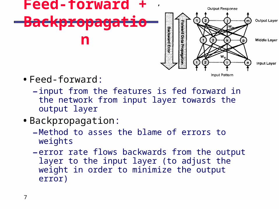
Feed-forward + Backpropagation

• Feed-forward: – input from the features is fed forward in the

network from input layer towards the output layer

• Backpropagation: –Method to asses the blame of errors to weights–error rate flows backwards from the output

layer to the input layer (to adjust the weight in order to minimize the output error)

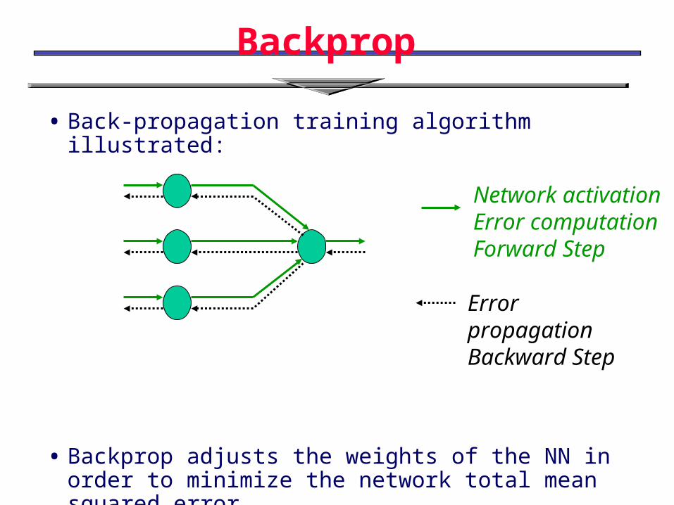
Backprop

• Back-propagation training algorithm illustrated:

• Backprop adjusts the weights of the NN in order to minimize the network total mean squared error.

Network activationError computationForward Step

Error propagationBackward Step

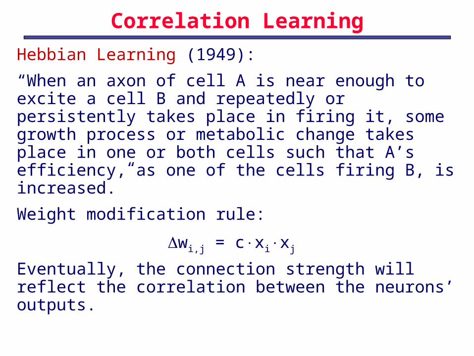
Correlation Learning

Hebbian Learning (1949):

“When an axon of cell A is near enough to excite a cell B and repeatedly or persistently takes place in firing it, some growth process or metabolic change takes place in one or both cells such that A’s efficiency, as one of the cells firing B, is increased.”

Weight modification rule:

wi,j = cxixj

Eventually, the connection strength will reflect the correlation between the neurons’ outputs.

10

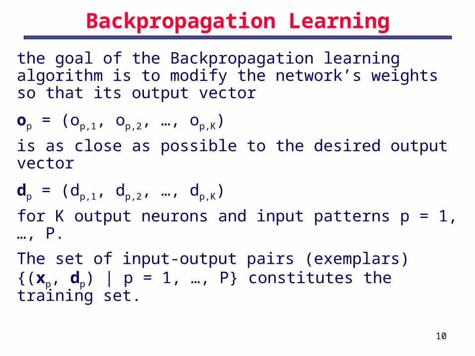
Backpropagation Learning

the goal of the Backpropagation learning algorithm is to modify the network’s weights so that its output vector

op = (op,1, op,2, …, op,K)

is as close as possible to the desired output vector

dp = (dp,1, dp,2, …, dp,K)

for K output neurons and input patterns p = 1, …, P.

The set of input-output pairs (exemplars) {(xp, dp) | p = 1, …, P} constitutes the training set.

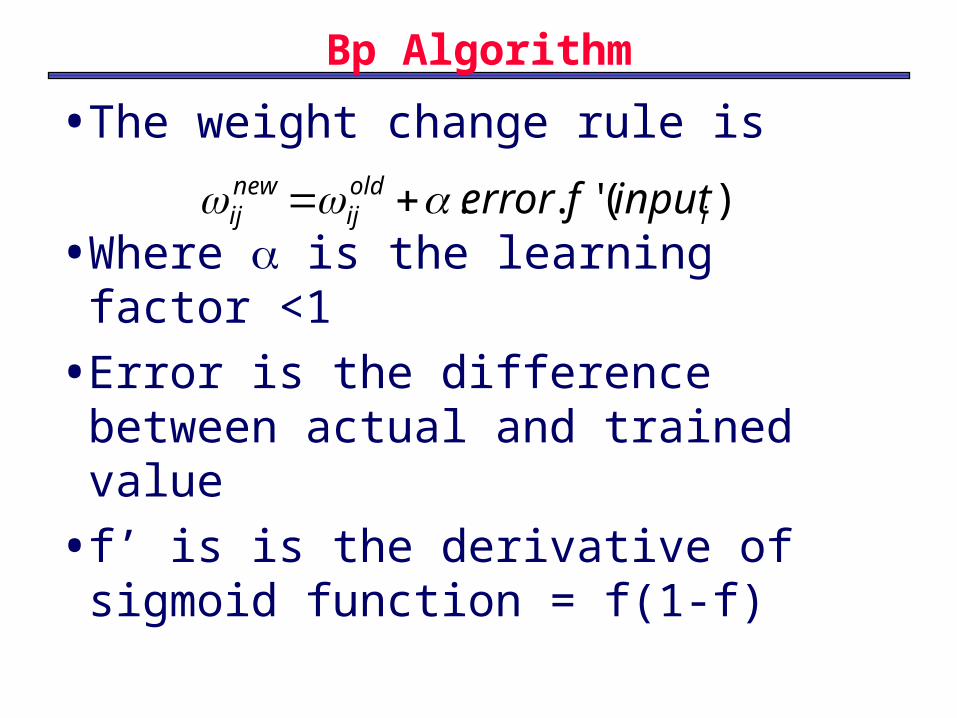
Bp Algorithm

• The weight change rule is

• Where is the learning factor <1

• Error is the difference between actual and trained value

• f’ is is the derivative of sigmoid function = f(1-f)

)('.. ioldij

newij inputferror

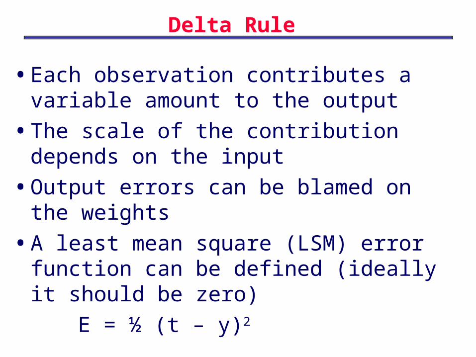
Delta Rule

• Each observation contributes a variable amount to the output

• The scale of the contribution depends on the input

• Output errors can be blamed on the weights

• A least mean square (LSM) error function can be defined (ideally it should be zero)

E = ½ (t – y)2

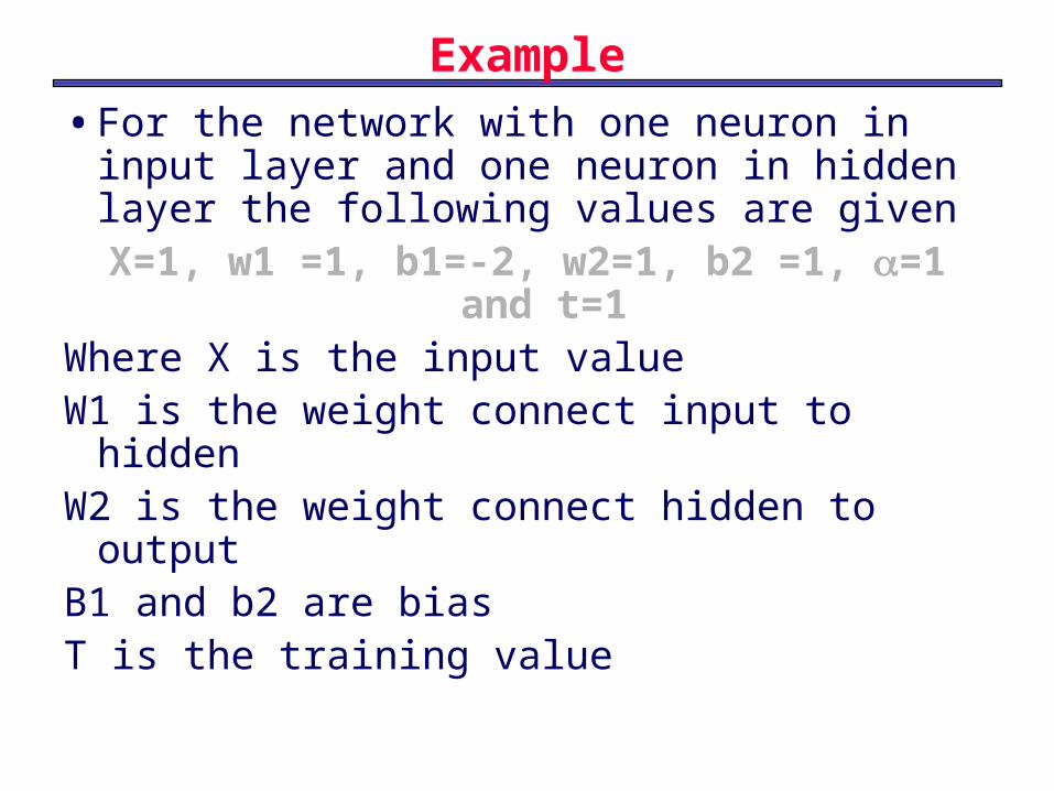
Example

• For the network with one neuron in input layer and one neuron in hidden layer the following values are given

X=1, w1 =1, b1=-2, w2=1, b2 =1, =1 and t=1

Where X is the input valueW1 is the weight connect input to hidden W2 is the weight connect hidden to outputB1 and b2 are biasT is the training value

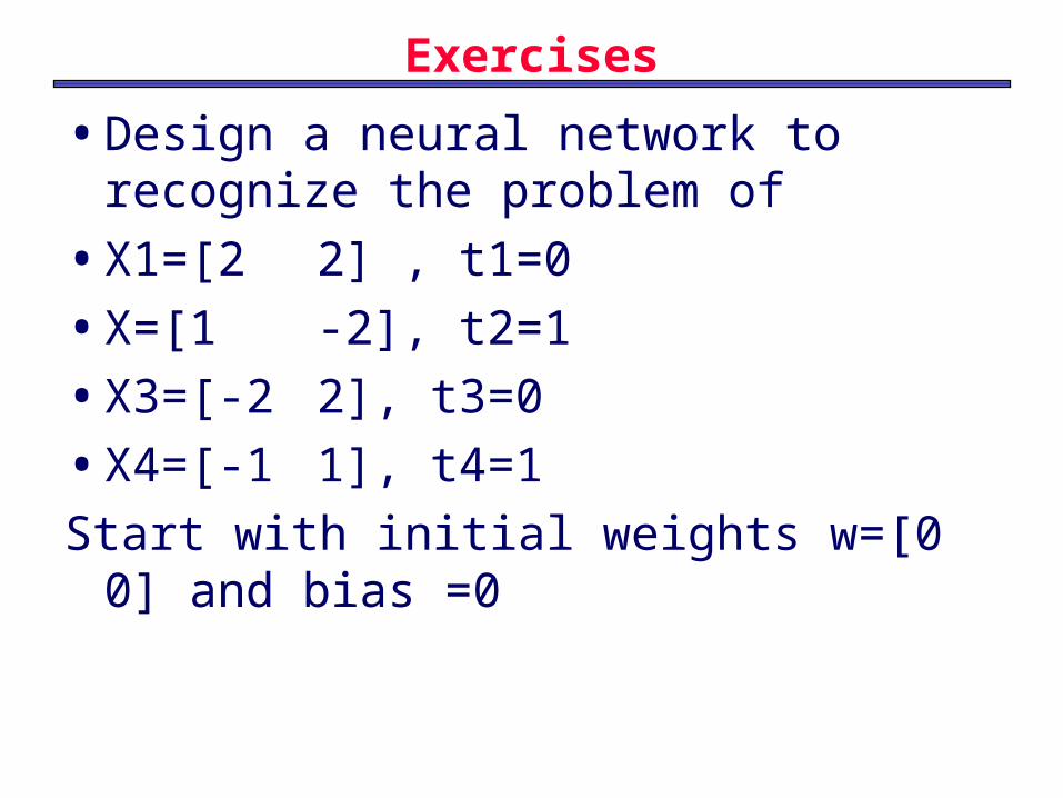
Exercises

• Design a neural network to recognize the problem of

• X1=[2 2] , t1=0

• X=[1 -2], t2=1

• X3=[-2 2], t3=0

• X4=[-1 1], t4=1

Start with initial weights w=[0 0] and bias =0

Exercises

• Perform one iteration of backprpgation to network of two layers. First layer has one neuron with weight 1 and bias –2. The transfer function in first layer is f=n2

• The second layer has only one neuron with weight 1 and bias 1. The f in second layer is 1/n.

• The input to the network is x=1 and t=1

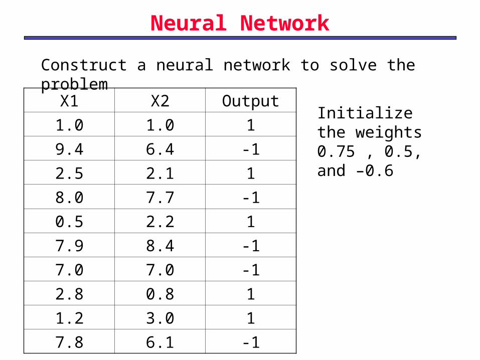
Neural Network

Construct a neural network to solve the problem

X1 X2 Output

1.0 1.0 1

9.4 6.4 -1

2.5 2.1 1

8.0 7.7 -1

0.5 2.2 1

7.9 8.4 -1

7.0 7.0 -1

2.8 0.8 1

1.2 3.0 1

7.8 6.1 -1

Initialize the weights 0.75 , 0.5, and –0.6

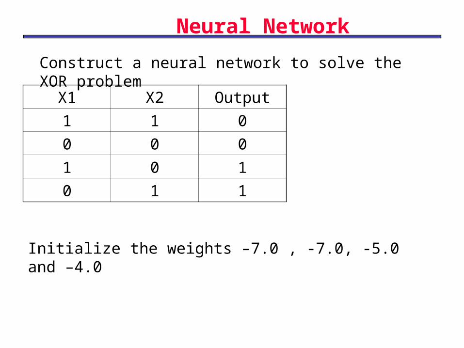
Neural Network

Construct a neural network to solve the XOR problem

X1 X2 Output

1 1 0

0 0 0

1 0 1

0 1 1

Initialize the weights –7.0 , -7.0, -5.0 and –4.0

-0.5

-0.5

-2

3

-1

1

1

1-1

1

0.5

The transfer function is linear function.

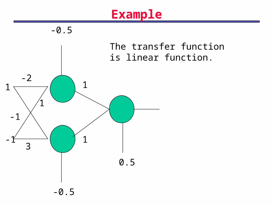
Example

Example

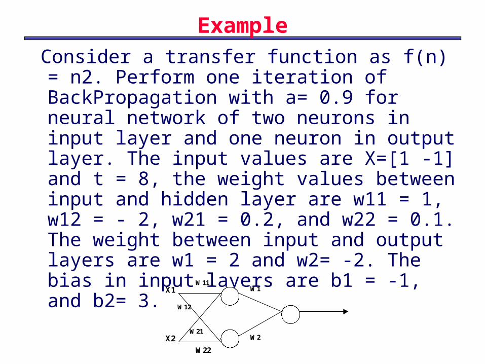
Consider a transfer function as f(n) = n2. Perform one iteration of BackPropagation with a= 0.9 for neural network of two neurons in input layer and one neuron in output layer. The input values are X=[1 -1] and t = 8, the weight values between input and hidden layer are w11 = 1, w12 = - 2, w21 = 0.2, and w22 = 0.1. The weight between input and output layers are w1 = 2 and w2= -2. The bias in input layers are b1 = -1, and b2= 3.

X1

X2

W11

W22

W12

W1

W21 W2

20

Some variations

• learning rate (). If is too small then learning is very slow. If large, then the system's learning may never converge.

• Some of the possible solutions to this problem are:– Add a momentum term to allow a large learning rate.

– Use a different activation function

– Use a different error function

– Use an adaptive learning rate

– Use a good weight initialization procedure.

– Use a different minimization procedure

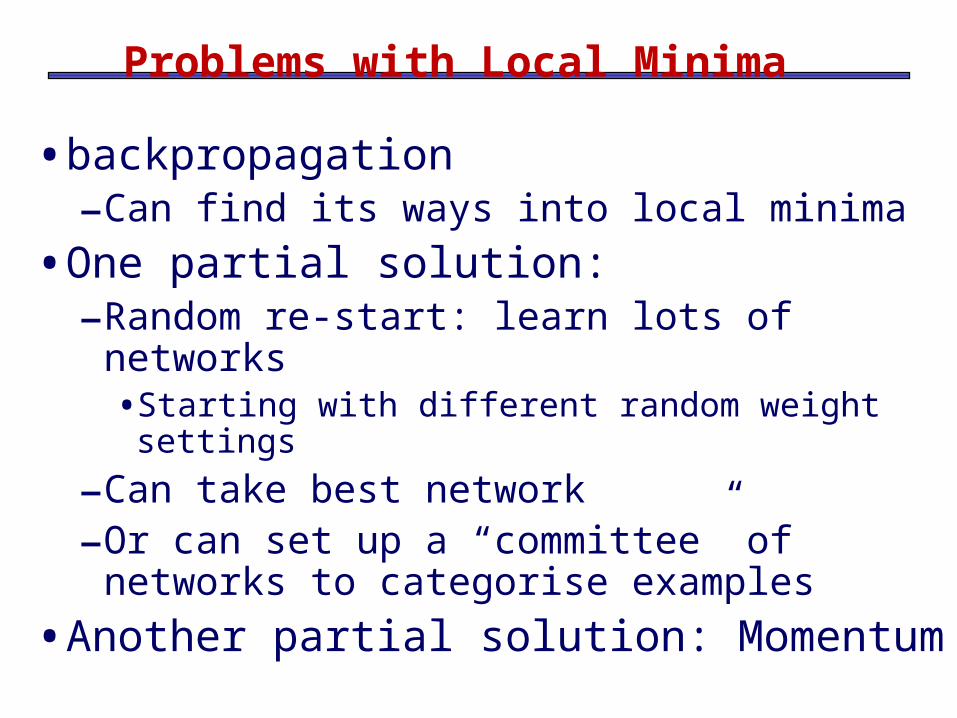
Problems with Local Minima

• backpropagation–Can find its ways into local minima

• One partial solution:–Random re-start: learn lots of networks

• Starting with different random weight settings

–Can take best network–Or can set up a “committee” of networks to

categorise examples

• Another partial solution: Momentum

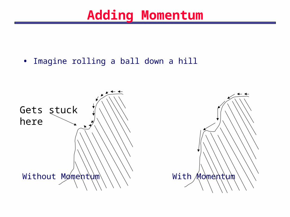
Adding Momentum

• Imagine rolling a ball down a hill

Without Momentum With Momentum

Gets stuck here

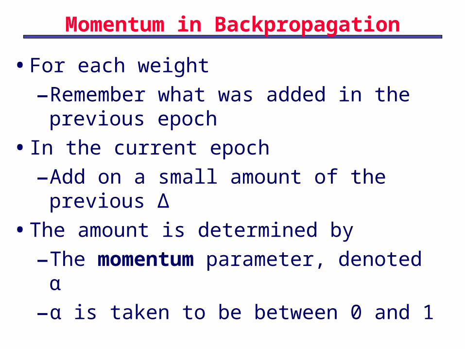
Momentum in Backpropagation

• For each weight

–Remember what was added in the previous epoch

• In the current epoch

–Add on a small amount of the previous Δ

• The amount is determined by

–The momentum parameter, denoted α

–α is taken to be between 0 and 1

24

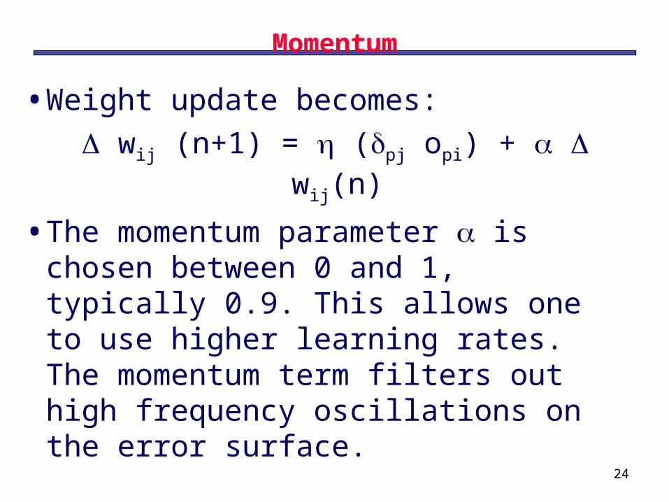
Momentum

• Weight update becomes:

wij (n+1) = (pj opi) + wij(n)

• The momentum parameter is chosen between 0 and 1, typically 0.9. This allows one to use higher learning rates. The momentum term filters out high frequency oscillations on the error surface.

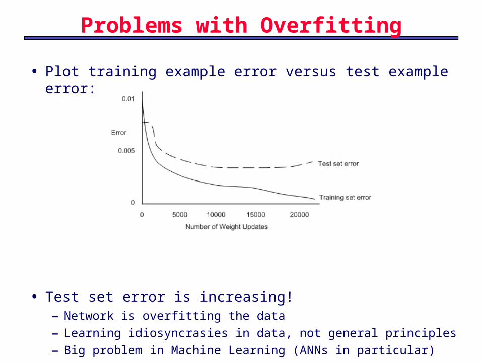
Problems with Overfitting

• Plot training example error versus test example error:

• Test set error is increasing!– Network is overfitting the data

– Learning idiosyncrasies in data, not general principles

– Big problem in Machine Learning (ANNs in particular)

Avoiding Overfitting• Bad idea to use training set accuracy to terminate• One alternative: Use a validation set

–Hold back some of the training set during training–Like a miniature test set (not used to train weights

at all)– If the validation set error stops decreasing, but the

training set error continues decreasing• Then it’s likely that overfitting has started to occur, so

stop

• Another alternative: use a weight decay factor–Take a small amount off every weight after each

epoch–Networks with smaller weights aren’t as highly fine

tuned (overfit)

Feedback NN

Recurrent Neural Networks

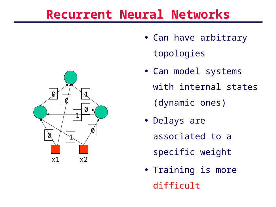
Recurrent Neural Networks

• Can have arbitrary

topologies

• Can model systems with

internal states (dynamic

ones)

• Delays are associated to

a specific weight

• Training is more difficultx1 x2

1

010

10

00

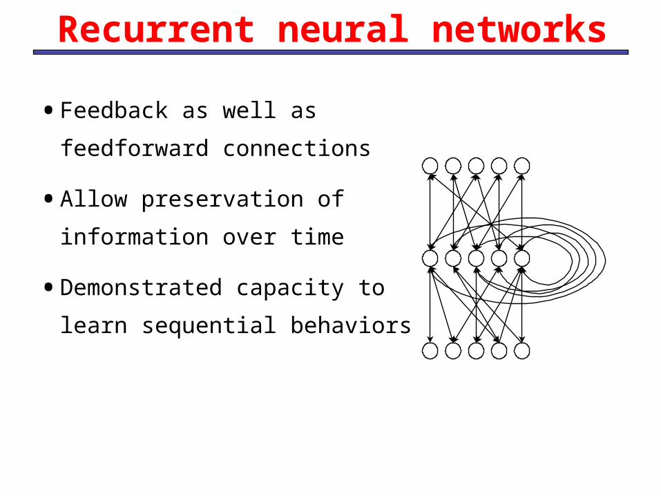
Recurrent neural networks

• Feedback as well as

feedforward connections

• Allow preservation of

information over time

• Demonstrated capacity to learn

sequential behaviors

30

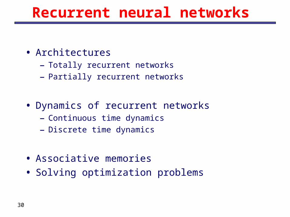
Recurrent neural networks

• Architectures– Totally recurrent networks

– Partially recurrent networks

• Dynamics of recurrent networks– Continuous time dynamics

– Discrete time dynamics

• Associative memories

• Solving optimization problems

Input-Output Recurrent Model• Input-Output Recurrent

Model → nonlinear autoregressive with exogeneous inputs model (NARX) y(n+1) = F(y(n),...,y(n-q+1),u(n),...,u(n-q+1))

• The model has a single input. It has a single output that is fed back to the input.

• The present value of the model input is denoted u(n), and the corresponding value of the model output is denoted by y(n+1).

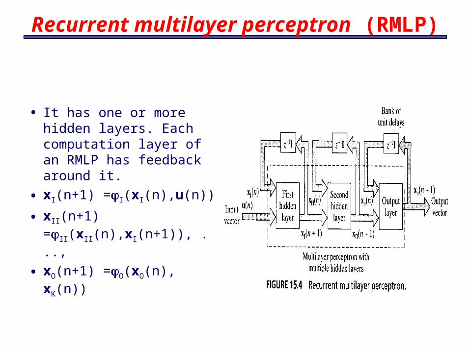
Recurrent multilayer perceptron (RMLP)

• It has one or more hidden layers. Each computation layer of an RMLP has feedback around it.

• xI(n+1) =I(xI(n),u(n))

• xII(n+1) =II(xII(n),xI(n+1)), ...,

• xO(n+1) =O(xO(n), xK(n))

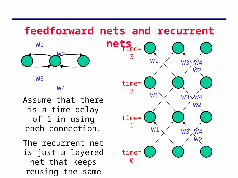
The equivalence between layered,

feedforward nets and recurrent netsw1 w2

w3 w4

w1 w2w3 w4

w1 w2w3 w4

w1 w2w3 w4

time=0

time=2

time=1

time=3

Assume that there is a time delay of 1 in using

each connection.

The recurrent net is just a layered net that

keeps reusing the same weights.

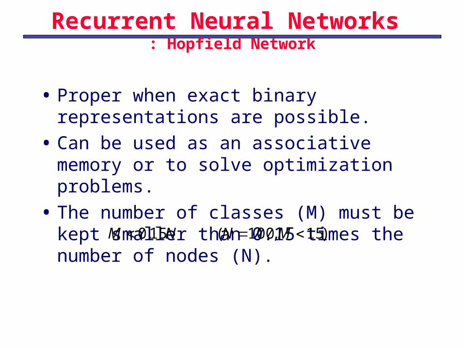
Recurrent Neural Networks : Hopfield Network

• Proper when exact binary representations are possible.

• Can be used as an associative memory or to solve optimization problems.

• The number of classes (M) must be kept smaller than 0.15 times the number of nodes (N). )15,100(15.0 MNNM

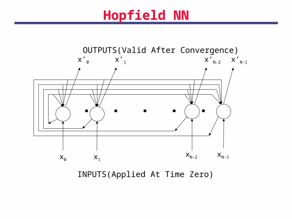
x0 x1xN-2 xN-1

x’0 x’1 x’N-2 x’N-1

. . . . .

INPUTS(Applied At Time Zero)

OUTPUTS(Valid After Convergence)

Hopfield NN

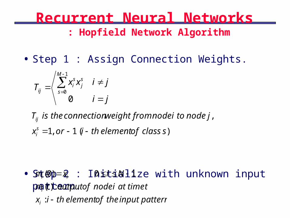
Recurrent Neural Networks : Hopfield Network Algorithm

• Step 1 : Assign Connection Weights.

• Step 2 : Initialize with unknown input pattern.

ji

jixxT

M

s

sj

si

ij

0

1

0

)(1,1

,

sclassofelementthiorx

jnodetoinodefromweightconnectiontheisTsi

ij

patterninputtheofelementthix

ttimeatinodeofoutputtm

Nixm

i

i

ii

:

:)(

10)0(

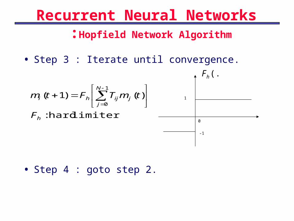
• Step 3 : Iterate until convergence.

• Step 4 : goto step 2.

limiter hard:

)()1(1

0

h

N

jjijhi

F

tmTFtm

1

0

-1

(.)hF

Recurrent Neural Networks :Hopfield Network Algorithm

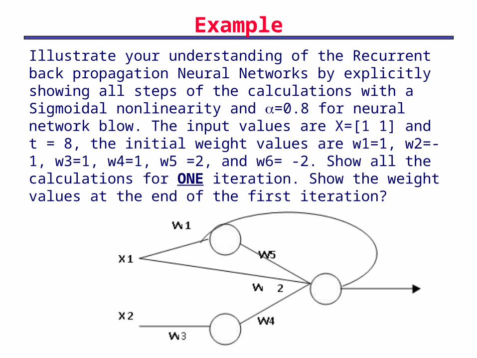
Example

Illustrate your understanding of the Recurrent back propagation Neural Networks by explicitly showing all steps of the calculations with a Sigmoidal nonlinearity and =0.8 for neural network blow. The input values are X=[1 1] and t = 8, the initial weight values are w1=1, w2=-1, w3=1, w4=1, w5 =2, and w6= -2. Show all the calculations for ONE iteration. Show the weight values at the end of the first iteration?

39

ne 1

1

2)(2

1yt

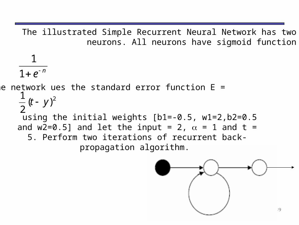
The illustrated Simple Recurrent Neural Network has two neurons. All neurons have sigmoid function

. The network ues the standard error function E =

using the initial weights [b1=-0.5, w1=2,b2=0.5 and w2=0.5] and let the input = 2, = 1 and t = 5. Perform two iterations of recurrent back-

propagation algorithm.

Unsupervised Learning

•Supervised learning, in which an external teacher improves

network performance by comparing desired and actual

outputs and modifying the synaptic weights accordingly.

•However, most of the learning that takes place in our brains

is completely unsupervised.

•This type of learning is aimed at achieving the most efficient

representation of the input space, regardless of any output

space.

Unsupervised learning

• The network must discover for itself patterns, features, regularities,correlations or categories in the input data and code them for the output.

• The units and connections must self-organize themselves based on the stimulus they receive.

• Note that unsupervised learning is useful when there is redundancy in the input data. Redundancy provides knowledge.

Unsupervised Learning

•Applications of unsupervised learning include

•Clustering

•Vector quantization

•Data compression

•Feature extraction

Self-organising maps (SOMs)

• Inspiration from Biology: In auditory pathway

nerve cells arranged in relation to frequency

response (tonotopic organisation).

• Kohonen took inspiration from to produce self-

organising maps (SOMs).

• In SOM units located physically next to one

another will respond to input vectors that are

‘similar’.

SOMs

• Useful, as difficult for Humans to visualise when

data has > 3 dimensions.

• Large dimensional input vectors 'projected down'

onto 2-D map in way maintaining natural order

similarity.

• SOM is 2-D array of neurons, all inputs arriving

at all neurons .

SOMs

• Initially each neuron has own set of (random)

weights.

• When input arrives neuron with pattern of

weights most similar to input gives largest

response.

SOMs

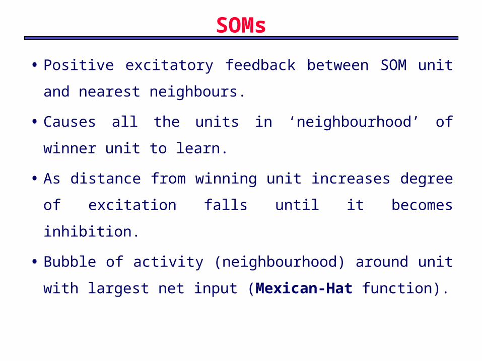
• Positive excitatory feedback between SOM unit

and nearest neighbours.

• Causes all the units in ‘neighbourhood’ of winner

unit to learn. 

• As distance from winning unit increases degree of

excitation falls until it becomes inhibition.

• Bubble of activity (neighbourhood) around unit

with largest net input (Mexican-Hat function).

SOMs

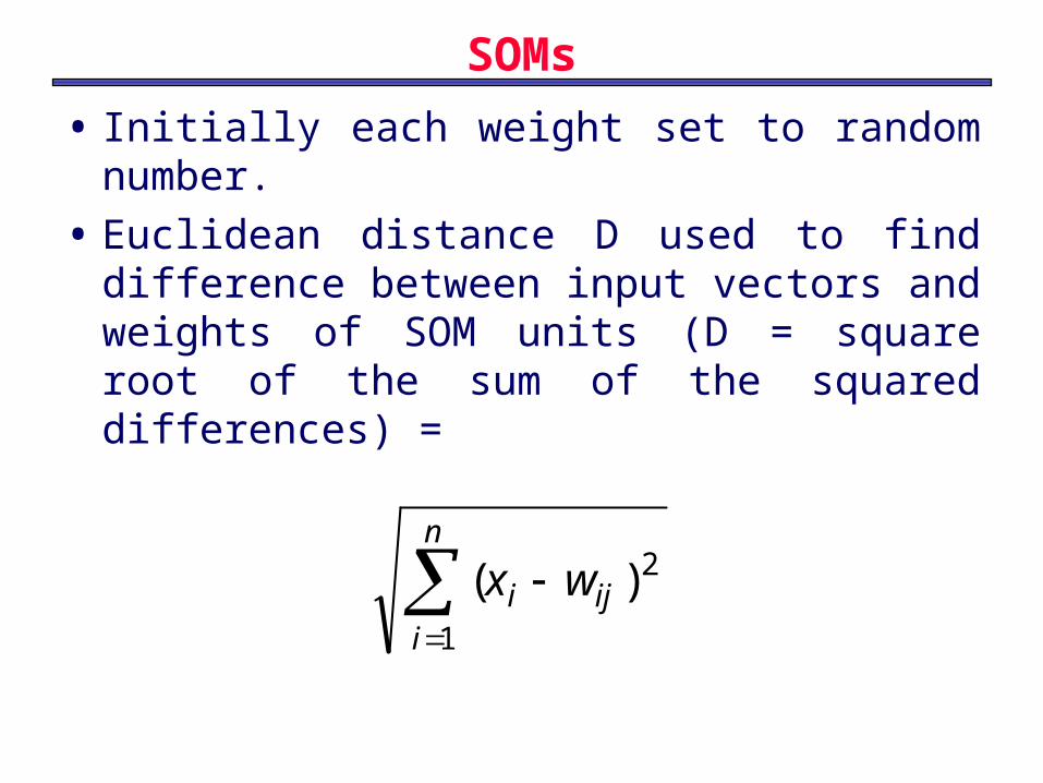
• Initially each weight set to random number.

• Euclidean distance D used to find difference between input vectors and weights of SOM units (D = square root of the sum of the squared differences) =

n

iiji wx

1

2)(

SOMs

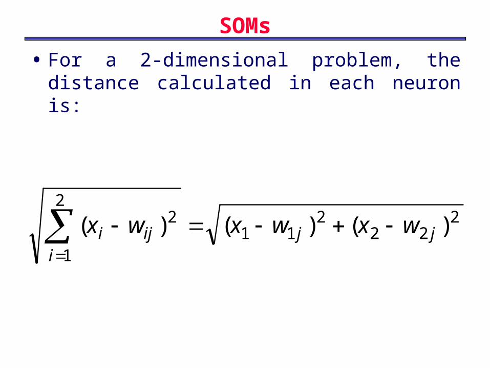
• For a 2-dimensional problem, the distance calculated in each neuron is:

222

211

2

1

2 )()()( jji

iji wxwxwx

SOM

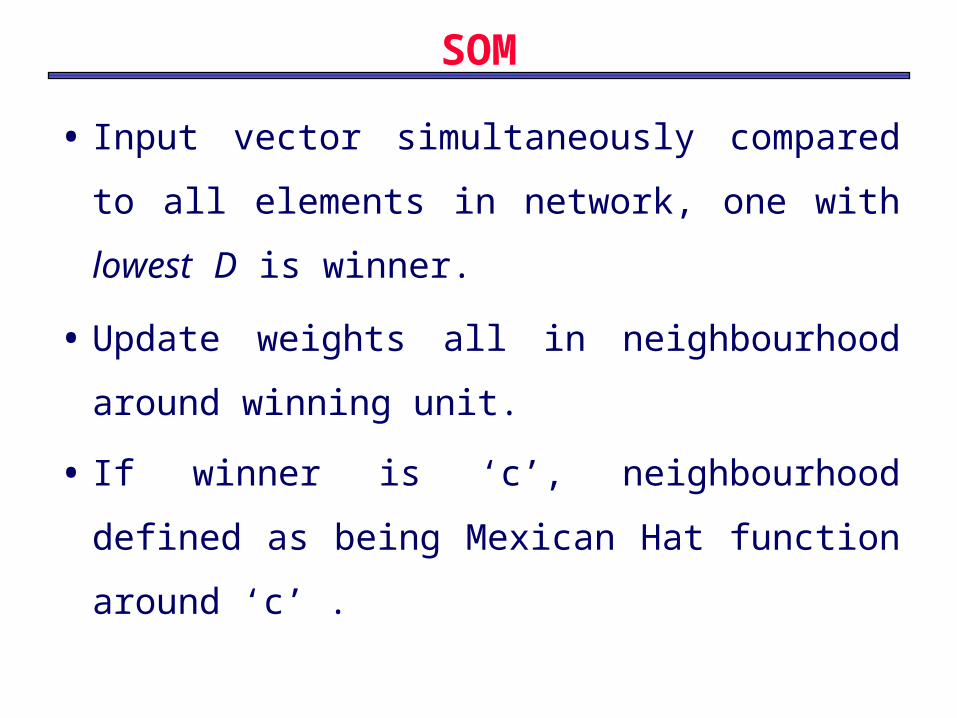
• Input vector simultaneously compared to all

elements in network, one with lowest D is

winner. 

• Update weights all in neighbourhood around

winning unit. 

• If winner is ‘c’, neighbourhood defined as being

Mexican Hat function around ‘c’ .

SOMs

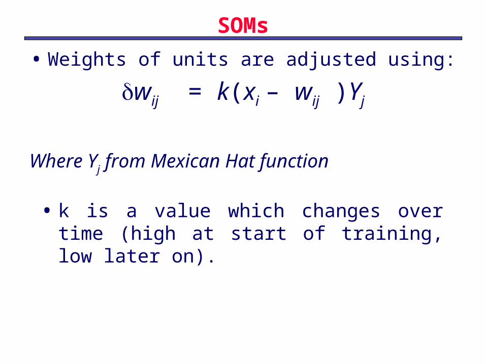
• Weights of units are adjusted using:

wij = k(xi – wij )Yj

Where Yj from Mexican Hat function

• k is a value which changes over time (high at start of training, low later on).

Two distinct phases in training

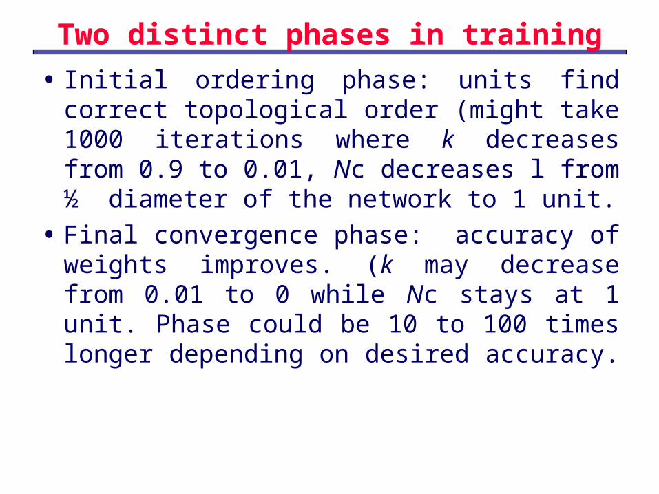
• Initial ordering phase: units find correct topological order (might take 1000 iterations where k decreases from 0.9 to 0.01, Nc decreases l from ½ diameter of the network to 1 unit.

• Final convergence phase: accuracy of weights improves. (k may decrease from 0.01 to 0 while Nc stays at 1 unit. Phase could be 10 to 100 times longer depending on desired accuracy.

53

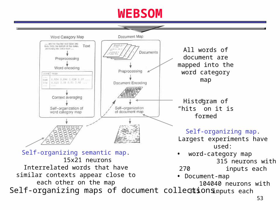
WEBSOM

All words of document are

mapped into the word category map

Histogram of “hits” on it is formed

Self-organizing map.Largest experiments have used:

• word-category map315 neurons with 270

inputs each• Document-map

104040 neurons with 315 inputs each

Self-organizing semantic map.15x21 neurons

Interrelated words that have similar contexts appear close to each other on the map

Self-organizing maps of document collections.

NN 4 54

WEBSOM

Clustering Data

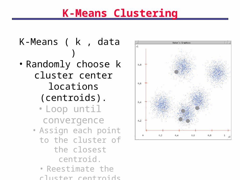
K-Means Clustering

K-Means ( k , data )• Randomly choose k

cluster center locations

(centroids).• Loop until convergence

• Assign each point to the cluster of the closest centroid.

• Reestimate the cluster centroids based on the data assigned to each.

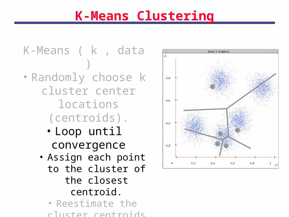
K-Means Clustering

K-Means ( k , data )• Randomly choose k

cluster center locations

(centroids).• Loop until convergence

• Assign each point to the cluster of the closest centroid.

• Reestimate the cluster centroids based on the data assigned to each.

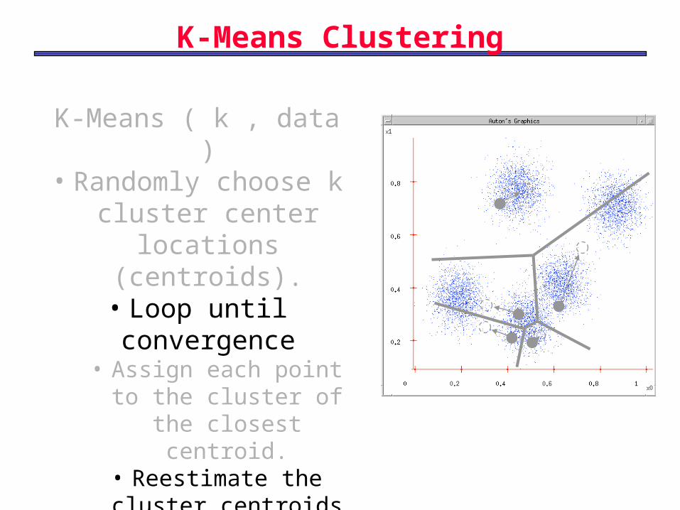
K-Means Clustering

K-Means ( k , data )• Randomly choose k

cluster center locations

(centroids).• Loop until convergence

• Assign each point to the cluster of the closest centroid.

• Reestimate the cluster centroids based on the data assigned to each.

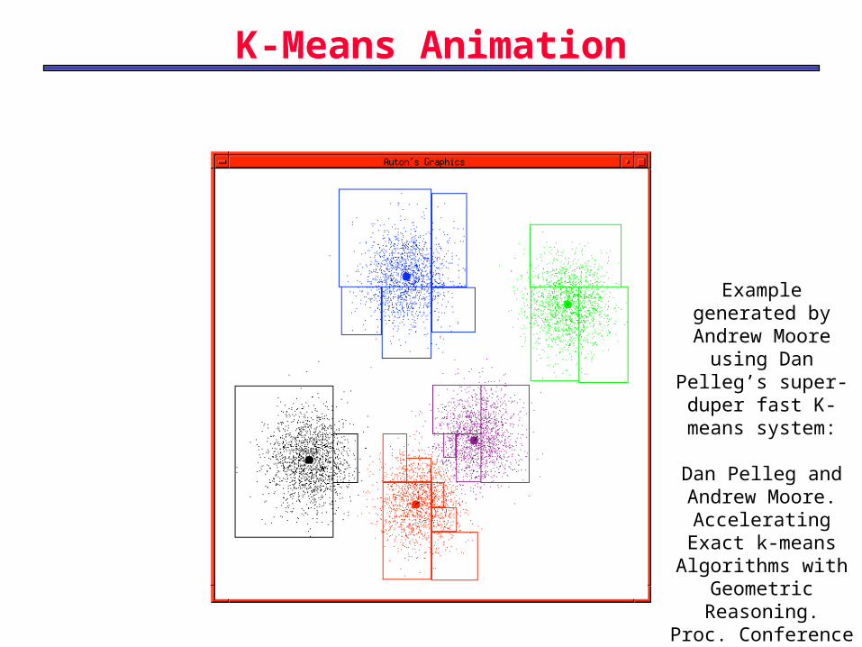
K-Means Animation

Example generated by

Andrew Moore using Dan Pelleg’s super-duper fast K-means system:

Dan Pelleg and Andrew Moore.

Accelerating Exact k-means

Algorithms with Geometric Reasoning.

Proc. Conference on

Knowledge Discovery in

Databases 1999.

60

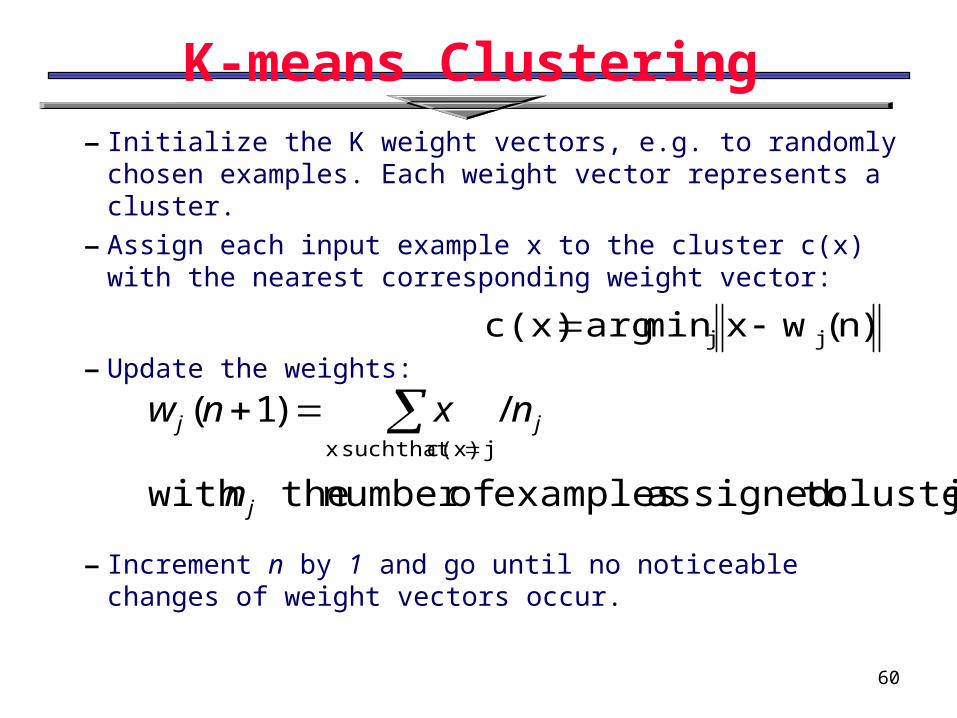
K-means Clustering

– Initialize the K weight vectors, e.g. to randomly chosen examples. Each weight vector represents a cluster.

– Assign each input example x to the cluster c(x) with the nearest corresponding weight vector:

– Update the weights:

– Increment n by 1 and go until no noticeable changes of weight vectors occur.

)n(wxmin argc(x) jj

jcluster toassigned examples ofnumber the with

/)1(j c(x) that suchx

j

jj

n

nxnw

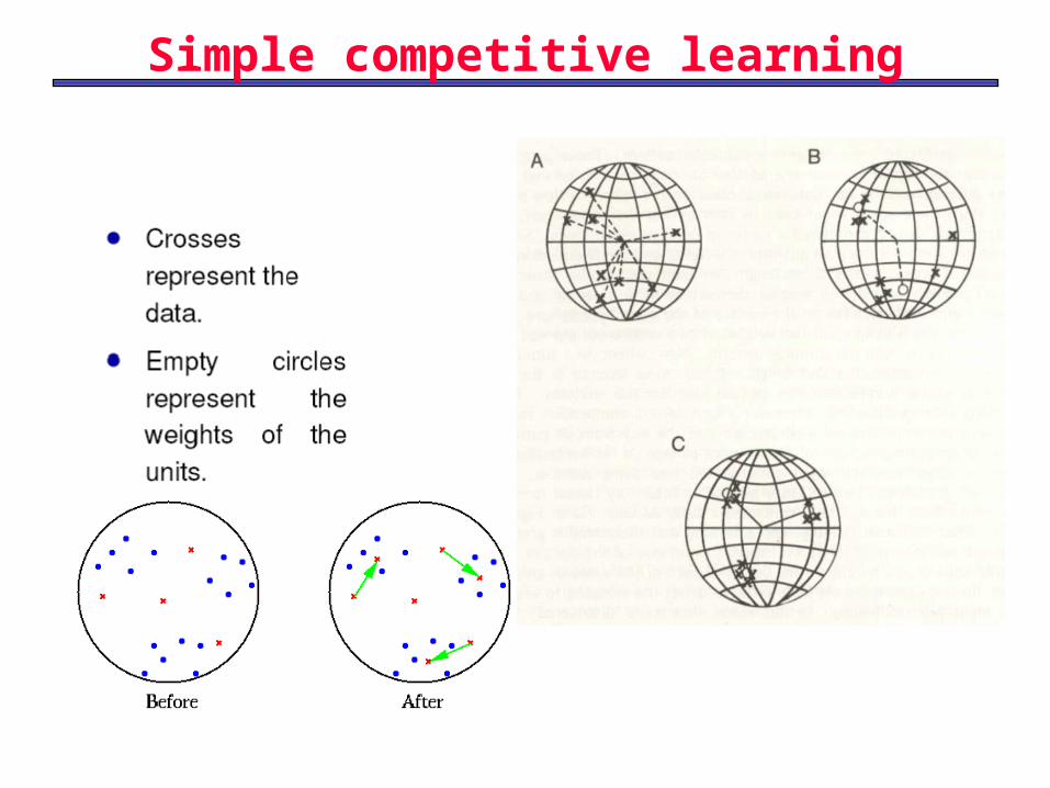
Simple competitive learning

62

Issues

• How many clusters?– User given parameter K– Use model selection criteria (Bayesian Information Criterion) with

penalization term which considers model complexity. See e.g. X-means: http://www2.cs.cmu.edu/~dpelleg/kmeans.html

• What similarity measure?– Euclidean distance– Correlation coefficient– Ad-hoc similarity measure

• How to assess the quality of a clustering?– Compact and well separated clusters are better … many different

quality measures have been introduced. See e.g. C. H. Chou, M. C. Su and E. Lai, “A New Cluster Validity Measure and Its Application to Image Compression,” Pattern Analysis and Applications, vol. 7, no. 2, pp. 205-220, 2004. (SCI)