Embed Size (px)
Citation preview

Machine Learning - MT 2016
11 & 12. Neural Networks
Varun Kanade
University of OxfordNovember 14 & 16, 2016

Announcements
I Problem Sheet 3 due this Friday by noon
I Practical 2 this week: Compare NBC & LR
I (Optional) Reading a paper
1

Outline
Today, we’ll study feedforward neural networks
I Multi-layer perceptrons
I Classification or regression settings
I Backpropagation to compute gradients
I Brief introduction to tensorflow and MNIST
2

Artificial Neuron : Logistic Regression
1
x1
x2
Σ y = Pr(y = 1 | x,w, b)
b
w1
w2
Non-linearity
Linear Function
Unit
I A unit in a neural network computes a linear function of its input and isthen composed with a non-linear activation function
I For logistic regression, the non-linear activation function is the sigmoid
σ(z) =1
1 + e−z
I The separating surface is linear
3

Multilayer Perceptron (MLP) : Classification
1
x1
x2
1
Σ
Σ
1 Σ y = Pr(y = 1 | x,W,b)
b21
w211
w212
b22
w221
w222
w311
w312
b31
4

Multilayer Perceptron (MLP) : Regression
1
x1
x2
1
Σ
Σ
1 Σ y = E[y | x,W,b]
b21
w211
w212
b22
w221
w222
w311
w312
b31
5

A Toy Example
6

Logistic Regression Fails Badly
7

Solve using MLP
1
x1
x2
1
Σ
Σ
z21 a2
1
z22 a2
2
1 Σ
z31 a3
1
y = Pr(y = 1 | x,Wi,bi)
b21
w211
w212
b22
w221
w222
w311
w312
b31
Let us use the notation:
a1 = z1 = x
z2 = W2a1 + b2
a2 = tanh(z2)
z3 = W3a2 + b3
y = a3 = σ(z3)
8

Scatterplot Comparison (x1, x2) vs (a21, a22)
9

Decision Boundary of the Neural Net
10

Feedforward Neural Networks
Layer 2(Hidden)
Layer 1(Input)
Layer 3(Hidden)
Layer 4(Output)
FullyConnected
Layer
11

Computing Gradients on Toy Example
x1
x2
z21 → a2
1
z22 → a2
2
z31 → a3
1 `(y, a31)
w211
w212
b21
w221
w222
b22
w311
w312
b31
Want the derivatives
∂`∂w2
11, ∂`∂w2
12
∂`∂w2
21, ∂`∂w2
22
∂`∂w3
11, ∂`∂w3
12
∂`∂b21
, ∂`∂b22
, ∂`∂b31
Would suffice to compute ∂`∂z31
, ∂`∂z21
, ∂`∂z22
12

Computing Gradients on Toy ExampleLet us compute the following:
1. ∂`∂a3
1= − y
a31
+ 1−y
1−a31
=a31−y
a31(1−a3
1)
2. ∂a3
∂z31= a3
1 · (1− a31)
3. ∂z31∂a2 = [w3
11, w312]
4. ∂a2
∂z2=
[1− tanh2(z2
1) 00 1− tanh2(z2
2)
]
Then we can calculate
∂`∂z31
= ∂`∂a3
1· ∂a3
1
∂z31= a3
1 − y
∂`∂z2
=
(∂`∂a3
1· ∂a3
1
∂z31
)· ∂z31∂a2 · ∂a2
∂z2= ∂`
∂z31· ∂z31∂a2 · ∂a2
∂z2
13

layer 2
layer l − 1
layer l
layer L− 1
layer L
a1input x ∂`∂z2
aLloss `
∂`∂zl
∂`∂zL
Each layer consists of a linear functionand non-linear activation
Layer l consists of the following:
zl = Wlal−1 + bl
al = fl(zl)
where fl is the non-linear activation inlayer l.
If there are nl units in layer l, thenWl isnl × nl−1
Backward pass to compute derivatives
14

layer 2
layer l − 1
layer l
layer L− 1
layer L
a1input x
aLloss `
Forward Equations
(1) a1 = x (input)
(2) zl = Wlal−1 + bl
(3) al = fl(zl)
(4) `(aL, y)
15

Output Layer
layer L (zL → aL)
aL−1 ∂`∂zL
aL
zL = WLaL−1 + bL
aL = fL(zL)
Loss: `(y,aL)
∂`∂zL
= ∂`∂aL · ∂aL
∂zL
If there are nL (output) units in layer L, then ∂`∂aL and ∂`
∂zLare row vectors
with nL elements and ∂aL
∂zLis the nL × nL Jacobian matrix:
∂aL
∂zL=
∂aL1
∂zL1
∂aL1
∂zL2· · · ∂aL
1
∂zLnL∂aL
2
∂zL1
∂aL2
∂zL2· · · ∂aL
2
∂zLnL
......
. . ....
∂aLnL
∂zL1
∂aLnL
∂zL2· · ·
∂aLnL
∂zLnL
If fL is applied element-wise, e.g., sigmoid then this matrix is diagonal
16

Back Propagation
layer l (zl → al)
al−1 ∂`∂zl
al ∂`∂zl+1
al (the inputs into layer l + 1)
zl+1 = Wl+1al + bl+1 (wl+1j,k weight on connection from kth
unit in layer l to jth unit in layer l+ 1)
al = f(zl) (f is a non-linearity)∂`
∂zl+1 (derivative passed from layer above)
∂`∂zl
= ∂`∂zl+1 · ∂zl+1
∂zl
= ∂`∂zl+1 · ∂zl+1
∂al · ∂al
∂zl
= ∂`∂zl+1 ·Wl+1 · ∂al
∂zl
17

Gradients with respect to parameters
layer l (zl → al)
al−1 ∂`∂zl
al ∂`∂zl+1
zl = Wlal−1 + bl (wlj,k weight on connection from kth
unit in layer l-1 to jth unit in layer l)∂`∂zl
(obtained using backpropagation)
Consider ∂`
∂wlij
= ∂`
∂zli· ∂zli∂wl
ij
= ∂`
∂zli· al−1
j
∂`
∂bli= ∂`
∂zli
More succinctly, we may write: ∂`∂Wl =
(al−1 ∂`
∂zl
)T∂`∂bl = ∂`
∂zl
18
layer 2
layer l − 1
layer l
layer L− 1
layer L
a1input x ∂`∂z2
aLloss `
∂`∂zl
∂`∂zL
Forward Equations
(1) a1 = x (input)
(2) zl = Wlal−1 + bl
(3) al = fl(zl)
(4) `(aL, y)
Back-propagation Equations
(1) Compute ∂`∂zL
= ∂`∂aL · ∂aL
∂zL
(2) ∂`∂zl
= ∂`∂zl+1 ·Wl+1 · ∂al
∂zl
(3) ∂`∂Wl =
(al−1 ∂`
∂zl
)T(4) ∂`
∂bl = ∂`∂zl
19

Computational Questions
What is the running time to compute the gradient for a single data point?
I As many matrix multiplications as there are fully connected layers
I Performed twice during forward and backward pass
What is the space requirement?
I Need to store vectors al, zl, and ∂`∂zl
for each layer
Can we process multiple examples together?
I Yes, if we minibatch, we perform tensor operations
I Make sure that all parameters fit in GPU memory
20

Training Deep Neural Networks
I Back-propagation gives gradient
I Stochastic gradient descent is the method of choice
I RegularisationI How do we add `1 or `2 regularisation?I Don’t regularise bias terms
I How about convergence?
I What did we learn in the last 10 years, that we didn’t know in the 80s?
21

Training Feedforward Deep NetworksLayer 2(Hidden)
Layer 1(Input)
Layer 3(Hidden)
Layer 4(Output)
Why do we get non-convex optimisation problem?
All units in a layer are symmetric, hence invariant to permutations22

A toy example
1
x ∈ −1, 1
Σ a21 Target is y = 1−x
2
z21 a2
1
w21
b21
Squared Loss Function
`(a21, y) = (a2
1 − y)2
∂`∂z21
= 2(a21 − y) · ∂a2
1
∂z21= 2(a2
1 − y)σ′(z21)
If x = −1, w21 ≈ 5, b21 ≈ 0, then σ′(z2
1) ≈ 0
Cross-Entropy Loss Function
`(a21, y) = −(y log a2
1 + (1− y) log(1− a21))
∂`∂z21
=a21−y
a21(1−a2
1)· ∂a2
1
∂z21= (a2
1 − y)
−8 −6 −4 −2 0 2 4 6 8
0
0.2
0.4
0.6
0.8
1
z21
23

Propagating Gradients Backwards
x = a11
1 1 1
Σ Σ Σ a41w2
1 w31 w4
1
b21 b31 b41
I Cross entropy loss: `(a41, y) = −(y log a4
1 + (1− y) log(1− a41))
I ∂`∂z41
= a41 − y
I ∂`∂z31
= ∂`∂z41· ∂z41∂a3
1· ∂a3
1
∂z31= (a4
1 − y) · w41 · σ′(z3
1)
I ∂`∂z21
= ∂`∂z31· ∂z31∂a2
1· ∂a2
1
∂z31= (a4
1 − y) · w41 · σ′(z3
1) · w31 · σ′(z2
1)
I Saturation: When the output of an artificial neuron is in the ‘flat’ part,e.g.,where σ′(z) ≈ 0 for sigmoid
I Vanishing Gradient Problem: Multiplying several σ′(zli) together makesthe gradient≈ 0, when we have a large number of layers
I For example, when using sigmoid activation, σ′(z) ∈ [0, 1/4]
24

Avoiding Saturation
Use rectified linear units
Rectifier non-linearityf(z) = max(0, z)
Rectified Linear Unit (ReLU)max(0,a ·w + b)
You can also use f(z) = |z|
Other variantsleaky ReLUs, parametric ReLUs −3 −2 −1 0 1 2 3
0
1
2
3
Rectifier
25

Initialising Weights and Biases
Initialising is important when minimisingnon-convex functions. We may get very differentresults depending on where we start theoptimisation.
Suppose we were using a sigmoid unit, how wouldyou initialise the weights?
I Suppose z =∑D
i=1 wiai
I E.g., choose wi ∈ [− 1√D, 1√
D] at random
What if it were a ReLU unit?
I You can initialise similarly
How about the biases?
I For sigmoid, can use 0 or a random valuearound 0
I For ReLU, should use a small positive constant
26

Avoiding Overfitting
Deep Neural Networks have a lot of parameters
I Fully connected layers with n1, n2, .., nL units have at leastn1n2 + n2n3 + · · ·+ nL−1nL parameters
I For Problem Sheet 4, you will be asked to train an MLP for digitrecognition with 2 million parameters and only 60,000 training images
I For image detection, one of the most famous models, the neural netused by Krizhevsky, Sutskever, Hinton (2012) has 60 million parametersand 1.2 million training images
I How do we prevent deep neural networks from overfitting?
27

Early Stopping
Maintain validation set and stop trainingwhen error on validation set stopsdecreasing.
What are the computational costs?
I Need to compute validation errorI Can do this every few iterations to
reduce overhead
What are the advantages?
I If validation error flattens, or startsincreasing can stop optimisation
I Prevents overfitting
See paper by Hardt, Recht and Singer (2015)
28

Add Data: Modified Data
Typically, getting additional data is either impossible or expensive
Fake the data!
Images can be translated slight, rotated slightly, change of brightness, etc.
Google Offline Translate trained on entirely fake data!
Google Research Blog
29

Add Data: Adversarial Training
Take trained (or partially trained model)
Create examples by modifications ‘‘imperceptible to the human eye’’, butwhere the model fails
Szegedy et al. and Goodfellow et al.
30

Other Ideas to Reduce Overfitting
Hard constraints on weights
Gradient Clipping
Inject noise into the system
Enforce sparsity in the neural network
Unsupervised Pre-training(Bengio et al.)
31

Bagging (Bootstrap Aggregation)
Bagging (Leo Breiman - 1994)
I Given datasetD = 〈(xi, yi)〉Ni=1, sampleD1,D2, · · · ,Dk of sizeN fromD with replacement
I Train classifiers f1, . . . , fk onD1, . . . ,Dk
I When predicting use majority (or average if using regression)
I Clearly this approach is not practical for deep networks
32

Dropout
I For input x each hidden unit with probability 1/2 independently
I Every input, will have a potentially different mask
I Potentially exponentially different models, but have ‘‘same weights’’
I After training whole network is used by halving all the weights
Srivastava, Hinton, Krizhevsky, 2014
33

Errors Made by MLP for Digit Recognition
34

Avoiding Overfitting
I Use parameter sharing a.k.a weight tying in the model
I Exploit invariances to translation, rotation, etc.
I Exploit locality in images, audio, text, etc.
I Convolutional Neural Networks (convnets)
35
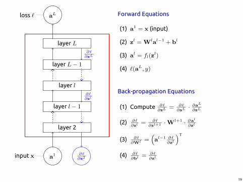
Convolutional Neural Networks (convnets)
(Fukushima, LeCun, Hinton 1980s)
36

Image Convolution
Source: L. W. Kheng
37

Convolution
In general, a convolution filter f is a tensor of dimensionWf ×Hf × Fl,where Fl is the number of channels in the previous layer
Strides in x and y directions dictate which convolutions are computed toobtain the next layer
Zero-padding can be used if required to adjust layer sizes and boundaries
Typically, a convolution layer will have a large number of filters, thenumber of channels in the next layer will be the same as the number offilters used
38

Source: Krizhevsky, Sutskever, Hinton (2012)
39

Sources: Krizhevsky, Sutskever, Hinton (2012); Wikipedia
40

Source: Krizhevsky, Sutskever, Hinton (2012)
41

Convolutional Layer
Suppose that there is no zero padding and strides in both directions are 1
zl+1i′,j′,f ′ = bf ′ +
Wf′∑i=1
Hf′∑j=1
Fl∑f=1
ali′+i−1,j′+j−1,fwl+1,f ′
i,j,f
∂zl+1i′,j′,f′
∂wl+1,f′i,j,f
= ali′+i−1,j′+j−1,f
∂`
∂wl+1,f′i,j,f
=∑i′,j′
∂`
∂zl+1i′,j′,f′
· ali′+i−1,j′+j−1,f
44

Convolutional Layer
Suppose that there is no zero padding and strides in both directions are 1
zl+1i′,j′,f ′ = bf ′ +
Wf′∑i=1
Hf′∑j=1
Fl∑f=1
ali′+i−1,j′+j−1,fwl+1,f ′
i,j,f
∂zl+1i′,j′,f′
∂ali,j,f
= wl+1,f ′
i−i′+1,j−j′+1,f
∂`
∂ali,j,f
=∑
i′,j′,f ′
∂`
∂zl+1i′,j′,f′
· wl+1,f ′
i−i′+1,j−j′+1,f
45
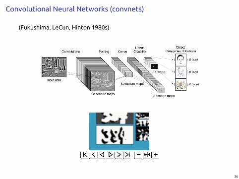
Max-Pooling Layer
Let Ω(i′, j′) be the set of (i, j) pairs in the previous layer that are involved inthe maxpool
sl+1i′,j′ = max
i,j∈Ω(i′,j′)ali,j
∂sl+1i′,j′
∂ali,j
= I
((i, j) = argmax
i,j∈Ω(i′,j′)
ali,j
)
46

Next Week
I Practial will be about training neural networks on MNIST dataset
I Time permitting, implement one problem on the sheet in tensorflow
I Start Unsupervised Learning
I Revise eigenvectors, eigenvalues (Problem 4 on Sheet 3)
47


![Machine Translation - 04: Neural Machine Translationhomepages.inf.ed.ac.uk/rsennric/mt18/4.pdf · R. Sennrich MT – 2018 – 04 12/20. Attention model [Cho et al., 2015] R. Sennrich](https://img.pdfslide.us/doc/110x75/603a4d2f2fca99785a286177/machine-translation-04-neural-machine-r-sennrich-mt-a-2018-a-04-1220-attention.jpg)