Machine Learning Lecture Notes

Predrag Radivojac

January 25, 2015

1 Basic Principles of Parameter Estimation

In probabilistic modeling, we are typically presented with a set of observationsand the objective is to find a model, or function, ˆM that shows good agreementwith the data and respects certain additional requirements. We shall roughlycategorize these requirements into three groups: (i) the ability to generalize well,(ii) the ability to incorporate prior knowledge and assumptions into modeling,and (iii) scalability. First, the model should be able to stand the test of time;that is, its performance on the previously unseen data should not deteriorateonce this new data is presented. Models with such performance are said togeneralize well. Second, ˆM must be able to incorporate information aboutthe model space M from which it is selected and the process of selecting amodel should be able to accept training “advice” from an analyst. Finally,when large amounts of data are available, learning algorithms must be ableto provide solutions in reasonable time given the resources such as memory orCPU power. In summary, the choice of a model ultimately depends on theobservations at hand, our experience with modeling real-life phenomena, andthe ability of algorithms to find good solutions given limited resources.

An easy way to think about finding the “best” model is through learningparameters of a distribution. Suppose we are given a set of observations D =

{xi

}ni=1, where x

i

2 R and have knowledge that M is a family of all univariateGaussian distributions, e.g. M = Gaussian(µ,�2

), with µ 2 R and � 2 R+. Inthis case, the problem of finding the best model (by which we mean function)can be seen as finding the best parameters µ⇤ and �⇤, i.e. the problem canbe seen as parameter estimation. We call this process estimation because thetypical assumption is that the data was generated by an unknown model fromM whose parameters we are trying to recover from data.

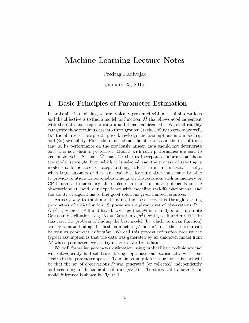
We will formalize parameter estimation using probabilistic techniques andwill subsequently find solutions through optimization, occasionally with con-strains in the parameter space. The main assumption throughout this part willbe that the set of observations D was generated (or collected) independentlyand according to the same distribution p

X

(x). The statistical framework formodel inference is shown in Figure 1.

1

Data generator Data set

Model

Parameter estimation

Observations Knowledge + Assumptions

Optimization

e.g.,

Experience

D= { }xi i= 1

nM, p M( ), ...

2 MMM p M p MMAP { ( | ) ( )= arg max }D

M E MB |= [ D = ]D

Model inference: Observations + + OptimizationKnowledge

andAssumptions

Figure 1: Statistical framework for model inference. The estimates of the pa-rameters are made using a set of observations D as well as experience in theform of model space M, prior distribution p(M), or specific starting solutionsin the optimization step.

2

1.1 Maximum a posteriori and maximum likelihood esti-

mation

The idea behind the maximum a posteriori (MAP) estimation is to find themost probable model for the observed data. Given the data set D, we formalizethe MAP solution as

MMAP

= argmax

M2M{p(M |D)} ,

where p(M |D) is the posterior distribution of the model given the data. Indiscrete model spaces, p(M |D) is the probability mass function and the MAPestimate is exactly the most probable model. Its counterpart in continuousspaces is the model with the largest value of the posterior density function.Note that we use words model, which is a function, and its parameters, whichare the coefficients of that function, somewhat interchangeably. However, weshould keep in mind the difference, even if only for pedantic reasons.

To calculate the posterior distribution we start by applying the Bayes ruleas

p(M |D) =

p(D|M) · p(M)

p(D)

, (1)

where p(D|M) is called the likelihood function, p(M) is the prior distributionof the model, and p(D) is the marginal distribution of the data. Notice that weuse D for the observed data set, but that we usually think of it as a realizationof a multidimensional random variable D drawn according to some distributionp(D). Using the formula of total probability, we can express p(D) as

p(D) =

8

>

<

>

:

P

M2M p(D|M)p(M) M : discrete

´M p(D|M)p(M)dM M : continuous

Therefore, the posterior distribution can be fully described using the likelihoodand the prior. The field of research and practice involving ways to determinethis distribution and optimal models is referred to as inferential statistics. Theposterior distribution is sometimes referred to as inverse probability.

Finding MMAP

can be greatly simplified because p(D) in the denominatordoes not affect the solution. We shall re-write Eq. (1) as

p(M |D) =

p(D|M) · p(M)

p(D)

/ p(D|M) · p(M),

where / is the proportionality symbol. Thus, we can find the MAP solution bysolving the following optimization problem

3

MMAP

= argmax

M2M{p(D|M)p(M)} .

In some situations we may not have a reason to prefer one model over anotherand can think of p(M) as a constant over the model space M. Then, themaximum a posteriori estimation reduces to the maximization of the likelihoodfunction; i.e.

MML

= argmax

M2M{p(D|M)} .

We will refer to this solution as the maximum likelihood solution. Formallyspeaking, the assumption that p(M) is constant is problematic because a uni-form distribution cannot be always defined (say, over R). Thus, it may be usefulto think of the maximum likelihood approach as a separate technique, ratherthan a special case of MAP estimation, with a conceptual caveat.

Observe that MAP and ML approaches report solutions corresponding tothe mode of the posterior distribution and the likelihood function, respectively.We shall later contrast this estimation technique with the view of the Bayesianstatistics in which the goal is to minimize the posterior risk. Such estimationtypically results in calculating conditional expectations, which can be complexintegration problems. From a different point of view, MAP and ML estimates arecalled point estimates, as opposed to estimated that report confidence intervalsfor particular group of parameters.

Example 8. Suppose data set D = {2, 5, 9, 5, 4, 8} is an i.i.d. sample froma Poisson distribution with an unknown parameter �

t

. Find the maximumlikelihood estimate of �

t

.The probability density function of a Poisson distribution is expressed as

p(x|�) = �xe��/x!, with some parameter � 2 R+. We will estimate this param-eter as

�ML

= argmax

�2(0,1){p(D|�)} .

We can write the likelihood function as

p(D|�) = p({xi

}ni=1 |�)

=

n

Y

i=1

p(xi

|�)

=

�P

n

i=1 x

i · e�n�

Q

n

i=1 xi

!

.

To find � that maximizes the likelihood, we will first take a logarithm (a mono-tonic function) to simplify the calculation, then find its first derivative withrespect to �, and finally equate it with zero to find the maximum. Specifically,we express the log-likelihood ll(D,�) = ln p(D|�) as

4

ll(D,�) = ln�n

X

i=1

xi

� n��n

X

i=1

ln (xi

!)

and proceed with the first derivative as

@ll(D,�)

@�=

1

�

n

X

i=1

xi

� n

= 0.

By substituting n = 6 and values from D, we can compute the solution as

�ML

=

1

n

n

X

i=1

xi

= 5.5,

which is simply a sample mean. The second derivative of the likelihood functionis always negative because � must be positive; thus, the previous expressionindeed maximizes the likelihood. We have ignored the anomalous cases when Dcontains all zeros.

⇤

Example 9. Let D = {2, 5, 9, 5, 4, 8} again be an i.i.d. sample fromPoisson(�

t

), but now we are also given additional information. Suppose theprior knowledge about �

t

can be expressed using a gamma distribution �(x|k, ✓)with parameters k = 3 and ✓ = 1. Find the maximum a posteriori estimate of�t

.First, we write the probability density function of the gamma family as

�(x|k, ✓) = xk�1e�x

✓

✓k�(k),

where x > 0, k > 0, and ✓ > 0. �(k) is the gamma function that generalizesthe factorial function; when k is an integer, we have �(k) = (k� 1)!. The MAPestimate of the parameters can be found as

�MAP

= argmax

�2(0,1){p(D|�)p(�)} .

As before, we can write the likelihood function as

p(D|�) = �P

n

i=1 x

i · e�n�

Q

n

i=1 xi

!

and the prior distribution as

5

p(�) =�k�1e�

�

✓

✓k�(k).

Now, we can maximize the logarithm of the posterior distribution p(�|D) using

ln p(�|D) / ln p(D|�) + ln p(�)

= ln�(k � 1 +

n

X

i=1

xi

)� �(n+

1

✓)�

n

X

i=1

lnxi

!� k ln ✓ � ln�(k)

to obtain

�MAP

=

k � 1 +

P

n

i=1 xi

n+

1✓

= 5

after incorporating all data.A quick look at �

MAP

and �ML

suggests that as n grows, both numeratorsand denominators in the expressions above become increasingly more similar.Unfortunately, equality between �

MAP

and �ML

when n ! 1 cannot be guar-anteed because it could occur by (a distant) chance that s

n

=

P

n

i=1 xi

does notgrow with n. One way to proceed is to calculate the expectation of the differencebetween �

MAP

and �ML

and then investigate what happens when n ! 1. Letus do this formally.

We shall first note that both estimates can be considered to be randomvariables. This follows from the fact that D is assumed to be an i.i.d. samplefrom a Poisson distribution with some true parameter �

t

. With this, we canwrite �

MAP

= (k � 1 + Sn

)/(n +

1✓

) and �ML

= Sn

/n, where Sn

=

P

n

i=1 Xi

and Xi

⇠ Poisson(�t

). We shall now prove the following convergence (in mean)result

lim

n!1E

D

[|�MAP

� �ML

|] = 0,

where the expectation is performed with respect to the random variable D. Letus first express the absolute difference between the two estimates as

|�MAP

� �ML

| =�

�

�

�

k � 1 + Sn

n+

1/✓� S

n

n

�

�

�

�

=

�

�

�

�

k � 1

n+

1/✓� S

n

n(n+

1/✓)

�

�

�

�

|k � 1|n+

1/✓+

Sn

n(n+

1/✓)

= ✏

where ✏ is a random variable that bounds the absolute difference between �MAP

and �ML

. We shall now express the expectation of ✏ as

6

E [✏] =1

n(n+

1/✓)· E

"

n

X

i=1

Xi

#

+

|k � 1|n+

1/✓

=

1

n+

1/✓· �

t

+

|k � 1|n+

1/✓

and therefore calculate that

lim

n!1E [✏] = 0.

This result shows that the MAP estimate approaches the ML solution for largedata sets. In other words, large data diminishes the importance of prior knowl-edge. This is an important conclusion because it simplifies mathematical appa-ratus necessary for practical inference. ⇤

1.1.1 The relationship with Kullback-Leibler divergence

We now investigate the relationship between maximum likelihood estimationand Kullback-Leibler divergence. Kullback-Leibler divergence between two prob-ability distributions p(x) and q(x) is defined as

DKL

(p||q) =ˆ 1

�1p(x) log

p(x)

q(x)dx.

In information theory, Kullback-Leibler divergence has a natural interpretationof the inefficiency of signal compression when the code is constructed using asuboptimal distribution q(x) instead of the correct (but unknown) distributionp(x) according to which the data has been generated. However, more oftenthan not, Kullback-Leibler divergence is simply considered to be a measure ofdivergence between two probability distributions. Although this divergence isnot a metric (it is not symmetric and does not satisfy the triangle inequality)it has important theoretical properties in that (i) it is always non-negative and(ii) it is equal to zero if and only if p(x) = q(x).

Consider now a divergence between an estimated probability distributionp(x|✓) and an underlying (true) distribution p(x|✓

t

) according to which thedata set D = {x

i

}ni=1 was generated. The Kullback-Leibler divergence between

p(x|✓) and p(x|✓t

) is

DKL

(p(x|✓t

)||p(x|✓)) =ˆ 1

�1p(x|✓

t

) log

p(x|✓t

)

p(x|✓) dx

=

ˆ 1

�1p(x|✓

t

) log

1

p(x|✓)dx�ˆ 1

�1p(x|✓

t

) log

1

p(x|✓t

)

dx.

The second term in the above equation is simply the entropy of the true distri-bution and is not influenced by our choice of the model ✓. The first term, onthe other hand, can be expressed as

7

ˆ 1

�1p(x|✓

t

) log

1

p(x|✓)dx = �E[log p(x|✓)]

Therefore, maximizing E[log p(x|✓)] minimizes the Kullback-Leibler divergencebetween p(x|✓) and p(x|✓

t

). Using the strong law of large numbers, we knowthat

1

n

n

X

i=1

log p(xi

|✓) a.s.! E[log p(x|✓)]

when n ! 1. Thus, when the data set is sufficiently large, maximizing thelikelihood function minimizes the Kullback-Leibler divergence and leads to theconclusion that p(x|✓ML) = p(x|✓

t

), if the underlying assumptions are satisfied.Under reasonable conditions, we can infer from it that ✓ML = ✓

t

. This will holdfor families of distributions for which a set of parameters uniquely determinesthe probability distribution; e.g. it will not generally hold for mixtures of dis-tributions but we will discuss this situation later. This result is only one of themany connections between statistics and information theory.

1.2 Parameter estimation for mixtures of distributions

We now investigate parameter estimation for mixture models, which is mostcommonly carried out using the expectation-maximization (EM) algorithm. Asbefore, we are given a set of i.i.d. observations D = {x

i

}ni=1, with the goal of

estimating the parameters of the mixture distribution

p(x|✓) =m

X

j=1

wj

p(x|✓j

).

In the equation above, we used ✓ = (w1, w2, . . . , wm

, ✓1, ✓2, . . . , ✓m) to combineall parameters. Just to be more concrete, we shall assume that each p(x

i

|✓j

) isan exponential distribution with parameter �

j

, i.e. p(x|✓j

) = �j

e��

j

x, where�j

> 0. Finally, we shall assume that m is given and will address simultaneousestimation of ✓ and m later.

Let us attempt to find the maximum likelihood solution first. By pluggingthe formula for p(x|✓) into the likelihood function we obtain

p(D|✓) =n

Y

i=1

p(xi

|✓)

=

n

Y

i=1

0

@

m

X

j=1

wj

p(xi

|✓j

)

1

A , (2)

which, unfortunately, is difficult to maximize using differential calculus (why?).Note that although p(D|✓) has O(mn

) terms, it can be calculated in O(mn)time as a log-likelihood.

8

Before introducing the EM algorithm, let us for a moment present two hypo-thetical scenarios that will help us to understand the algorithm. First, supposethat information is available as to which mixing component generated whichdata point. That is, suppose that D = {(x

i

, yi

)}ni=1 is an i.i.d. sample from

some distribution pXY

(x, y), where y 2 Y = {1, 2, . . . ,m} specifies the mixingcomponent. How would the maximization be performed then? Let us write thelikelihood function as

p(D|✓) =n

Y

i=1

p(xi

, yi

|✓)

=

n

Y

i=1

p(xi

|yi

, ✓)p(yi

|✓)

=

n

Y

i=1

wy

i

p(xi

|✓y

i

), (3)

where wj

= pY

(j) = P (Y = j). The log-likelihood is

log p(D|✓) =n

X

i=1

(logwy

i

+ log p(xi

|✓y

i

))

=

m

X

j=1

nj

logwj

+

n

X

i=1

log p(xi

|✓y

i

),

where nj

is the number of data points in D generated by the j-th mixing com-ponent.

It is useful to observe here that when y = (y1, y2, . . . , yn) is known, the inter-nal summation operator in Eq. (2) disappears. More importantly, it follows thatEq. (3) can be maximized in a relatively straightforward manner. Let us showhow. To find w = (w1, w2, . . . , wm

) we need to solve a constrained optimizationproblem, which we will do by using the method of Lagrange multipliers. Weshall first form the Lagrangian function as

L(w,↵) =m

X

j=1

nj

logwj

+ ↵

0

@

m

X

j=1

wj

� 1

1

A

where ↵ is the Lagrange multiplier. Then, by setting @

@w

k

L(w,↵) = 0 for everyk 2 Y and @

@↵

L(w,↵) = 0, we derive that wk

= �n

k

↵

and ↵ = �n. Thus,

wk

=

1

n

n

X

i=1

I(yi

= k),

where I(·) is the indicator function. To find all ✓j

, we recall that we assumed a

9

mixture of exponential distributions. Thus, we proceed by setting

@

@�k

n

X

i=1

log p(xi

|�y

i

) = 0,

for each k 2 Y. We obtain that

�k

=

nk

P

n

i=1 I(yi = k) · xi

,

which is simply the inverse mean over those data points generated by the k-thmixture component. In summary, we observe that if the mixing component des-ignations y are known, the parameter estimation is greatly simplified. This wasachieved by decoupling the estimation of mixing proportions and all parametersof the mixing distributions.

In the second hypothetical scenario, suppose that parameters ✓ are known,and that we would like to estimate the best configuration of the mixture des-ignations y (one may be tempted to call them “class labels”). This task lookslike clustering in which cluster memberships need to be determined based onthe known set of mixing distributions and mixing probabilities. To do this wecan calculate the posterior distribution of y as

p(y|D, ✓) =n

Y

i=1

p(yi

|xi

, ✓)

=

n

Y

i=1

wy

i

p(xi

|✓y

i

)

P

m

j=1 wj

p(xi

|✓j

)

(4)

and subsequently find the best configuration out of mn possibilities. Obviously,because of the i.i.d. assumption each element y

i

can be estimated separatelyand, thus, this estimation can be completed in O(mn) time. The MAP estimatefor y

i

can be found as

yi

= argmax

y

i

2Y

(

wy

i

p(xi

|✓y

i

)

P

m

j=1 wj

p(xi

|✓j

)

)

for each i 2 {1, 2, . . . , n}.In reality, neither “class labels” y nor the parameters ✓ are known. Fortu-

nately, we have just seen that the optimization step is relatively straightforwardif one of them is known. Therefore, the intuition behind the EM algorithm is toform an iterative procedure by assuming that either y or ✓ is known and calcu-late the other. For example, we can initially pick some value for ✓, say ✓(0), andthen estimate y by computing p(y|D, ✓(0)) as in Eq. (4). We can refer to thisestimate as y(0). Using y(0) we can now refine the estimate of ✓ to ✓(1) usingEq. (3). We can then iterate these two steps until convergence. In the case ofmixture of exponential distributions, we arrive at the following algorithm:

10

1. Initialize �(0)k

and w(0)k

for 8k 2 Y

2. Calculate y(0)i

= argmax

k2Y

⇢

w

(0)k

p(xi

|�(0)k

)P

m

j=1 w

(0)j

p(xi

|�(0)j

)

�

for 8i 2 {1, 2, . . . , n}

3. Set t = 0

4. Repeat until convergence

(a) w(t+1)k

=

1n

P

n

i=1 I(y(t)i

= j)

(b) �(t+1)k

=

Pn

i=1 I(y(t)i

=k)P

n

i=1 I(y(t)i

=k)·xi

(c) t = t+ 1

(d) y(t+1)i

= argmax

k2Y

⇢

w

(t)k

p(xi

|�(t)k

)P

m

j=1 w

(t)j

p(xi

|�(t)j

)

�

5. Report �(t)k

and w(t)k

for 8k 2 Y

This procedure is not quite yet the EM algorithm; rather, it is a version of itreferred to as classification EM algorithm. In the next section we will introducethe EM algorithm.

1.2.1 The expectation-maximization algorithm

The previous procedure was designed to iteratively estimate class membershipsand parameters of the distribution. In reality, it is not necessary to compute y;after all, we only need to estimate ✓. To accomplish this, at each step t, we canuse p(y|D, ✓(t)) to maximize the expected log-likelihood of both D and y

EY[log p(D,y|✓)|✓(t)] =X

y

log p(D,y|✓)p(y|D, ✓(t)), (5)

which can be carried out by integrating the log-likelihood function of D and yover the posterior distribution for y in which the current values of the parameters✓(t) are assumbed to be known. We can now formulate the expression for theparameters in step t+ 1 as

✓(t+1)= argmax

✓

n

E[log p(D,y|✓)|✓(t)]o

. (6)

The formula above is all that is necessary to create the update rule for theEM algorithm. Note, however, that inside of it we always have to re-computeEY[log p(D,y|✓)|✓(t)] function because the parameters ✓(t) have been updatedfrom the previous step. We then can perform maximization. Hence the name“expectation-maximization”, although it is perfectly valid to think of the EMalgorithm as an interative maximization of expectation from Eq. (5), i.e. “ex-pectation maximization”.

We now proceed as follows

11

E[log p(D,y|✓)|✓(t)] =m

X

y1=1

· · ·m

X

y

n

=1

log p(D,y|✓)p(y|D, ✓(t))

=

m

X

y1=1

· · ·m

X

y

n

=1

n

X

i=1

log p(xi

, yi

|✓)n

Y

l=1

p(yl

|xl

, ✓(t))

=

m

X

y1=1

· · ·m

X

y

n

=1

n

X

i=1

log (wy

i

p(xi

|✓y

i

))

n

Y

l=1

p(yl

|xl

, ✓(t)).

After several simplification steps, that we omit for space reasons, the expectationof the likelihood can be written as

E[log p(D,y|✓)|✓(t)] =n

X

i=1

m

X

j=1

log (wj

p(xi

|✓j

)) pY

i

(j|xi

, ✓(t)),

from which we can see that w and {✓j

}mj=1 can be separately found. In the final

two steps, we will first derive the update rule for the mixing probabilities andthen by assuming the mixing distributions are exponential, derive the updaterules for their parameters.

To maximize E[log p(D,y|✓)|✓(t)] with respect to w, we observe that this isan instance of constrained optimization because it must hold that

P

m

i=1 wi

= 1.We will use the method of Lagrange multipliers; thus, for each k 2 Y we needto solve

@

@wk

0

@

m

X

j=1

logwj

n

X

i=1

pY

i

(j|xi

, ✓(t)) + ↵

0

@

m

X

j=1

wj

� 1

1

A

1

A

= 0,

where ↵ is the Lagrange multiplier. It is relatively straightforward to show that

w(t+1)k

=

1

n

n

X

i=1

pY

i

(k|xi

, ✓(t)). (7)

Similarly, to find the solution for the parameters of the mixture distributions,we obtain that

�(t+1)k

=

P

n

i=1 pYi

(k|xi

, ✓(t))P

n

i=1 xi

pY

i

(k|xi

, ✓(t))(8)

for k 2 Y. As previously shown, we have

pY

i

(k|xi

, ✓(t)) =w

(t)k

p(xi

|�(t)k

)

P

m

j=1 w(t)j

p(xi

|�(t)j

)

, (9)

which can be computed and stored as an n ⇥ m matrix. In summary, for themixture of m exponential distributions, we summarize the EM algorithm bycombining Eqs. (7-9) as follows:

12

1. Initialize �(0)k

and w(0)k

for 8k 2 Y

2. Set t = 0

3. Repeat until convergence

(a) pY

i

(k|xi

, ✓(t)) =w

(t)k

p(xi

|�(t)k

)P

m

j=1 w

(t)j

p(xi

|�(t)j

)for 8(i, k)

(b) w(t+1)k

=

1n

P

n

i=1 pYi

(k|xi

, ✓(t))

(c) �(t+1)k

=

Pn

i=1 p

Y

i

(k|xi

,✓

(t))Pn

i=1 x

i

p

Y

i

(k|xi

,✓

(t))

(d) t = t+ 1

4. Report �(t)k

and w(t)k

for 8k 2 Y

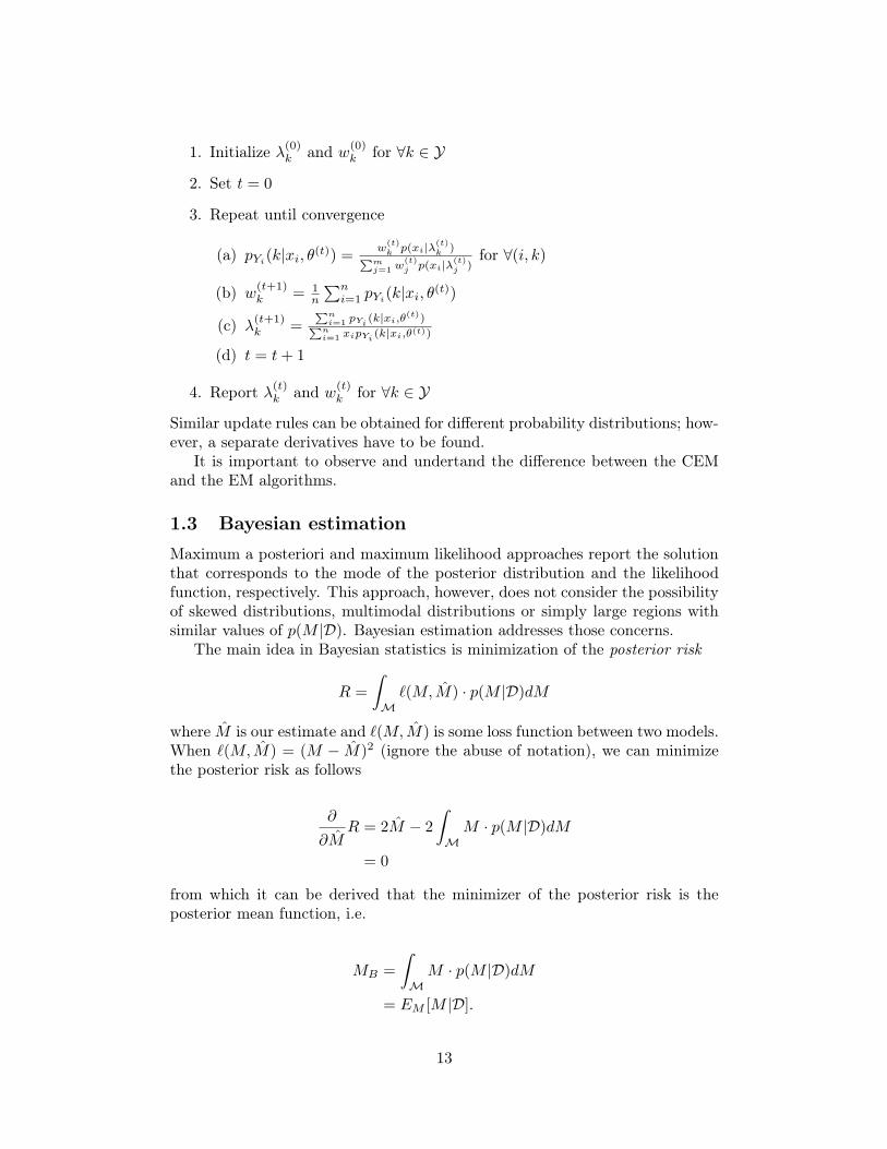
Similar update rules can be obtained for different probability distributions; how-ever, a separate derivatives have to be found.

It is important to observe and undertand the difference between the CEMand the EM algorithms.

1.3 Bayesian estimation

Maximum a posteriori and maximum likelihood approaches report the solutionthat corresponds to the mode of the posterior distribution and the likelihoodfunction, respectively. This approach, however, does not consider the possibilityof skewed distributions, multimodal distributions or simply large regions withsimilar values of p(M |D). Bayesian estimation addresses those concerns.

The main idea in Bayesian statistics is minimization of the posterior risk

R =

ˆM

`(M, ˆM) · p(M |D)dM

where ˆM is our estimate and `(M, ˆM) is some loss function between two models.When `(M, ˆM) = (M � ˆM)

2 (ignore the abuse of notation), we can minimizethe posterior risk as follows

@

@ ˆMR = 2

ˆM � 2

ˆM

M · p(M |D)dM

= 0

from which it can be derived that the minimizer of the posterior risk is theposterior mean function, i.e.

MB

=

ˆM

M · p(M |D)dM

= EM

[M |D].

13

We shall refer to MB

as the Bayes estimator. It is important to mention thatcomputing the posterior mean usually involves solving complex integrals. Insome situations, these integrals can be solved analytically; in others, numericalintegration is necessary.

Example 11. Let D = {2, 5, 9, 5, 4, 8} yet again be an i.i.d. sample fromPoisson(�

t

). Suppose the prior knowledge about the parameter of the exponen-tial distribution can be expressed using a gamma distribution with parametersk = 3 and ✓ = 1. Find the Bayesian estimate of �

t

.We want to find E[�|D]. Let us first write the posterior distribution as

p(�|D) =

p(D|�)p(�)p(D)

=

p(D|�)p(�)´10 p(D|�)p(�)d�

,

where, as shown in previous examples, we have that

p(D|�) = �P

n

i=1 x

i · e�n�

Q

n

i=1 xi

!

and

p(�) =�k�1e�

�

✓

✓k�(k).

Before calculating p(D), let us first note thatˆ 1

0x↵�1e��xdx =

�(↵)

�↵

.

Now, we can derive that

p(D) =

ˆ 1

0p(D|�)p(�)d�

=

ˆ 1

0

�P

n

i=1 x

i · e�n�

Q

n

i=1 xi

!

· �k�1e�

�

✓

✓k�(k)d�

=

�(k +

P

n

i=1 xi

)

✓k�(k)Q

n

i=1 xi

!(n+

1✓

)

Pn

i=1 x

i

+k

and subsequently that

14

p(�|D) =

p(D|�)p(�)p(D)

=

�P

n

i=1 x

i · e�n�

Q

n

i=1 xi

!

· �k�1e�

�

✓

✓k�(k)·✓k�(k)

Q

n

i=1 xi

!(n+

1✓

)

Pn

i=1 x

i

+k

�(k +

P

n

i=1 xi

)

=

�k�1+P

n

i=1 x

i · e��(n+1/✓) · (n+

1✓

)

Pn

i=1 x

i

+k

�(k +

P

n

i=1 xi

)

.

Finally,

E[�|D] =

ˆ 1

0�p(�|D)d�

=

k +

P

n

i=1 xi

n+

1✓

= 5.14

which is nearly the same solution as the MAP estimate found in Example 9. ⇤It is evident from the previous example that selection of the prior distribution

has important implications on calculation of the posterior mean. We have notpicked the gamma distribution by chance; that is, when the likelihood wasmultiplied by the prior, the resulting distribution remained in the same class offunctions as the likelihood. We shall refer to such prior distributions as conjugate

priors. Conjugate priors are also simplifying the mathematics; in fact, this is amajor reason for their consideration. Interestingly, in addition to the Poissondistribution, the gamma distribution is a conjugate prior to the exponentialdistribution as well as the gamma distribution itself.

15