Machine Learning in Ad-hoc IR. Machine Learning for ad hoc IR We’ve looked at methods for ranking documents in IR using factors like –Cosine similarity,

Machine Learning in Ad-hoc IR

Machine Learning for ad hoc IR• We’ve looked at methods for ranking documents in IR using

factors like– Cosine similarity, inverse document frequency, pivoted

document length normalization, Pagerank, etc.• We’ve looked at methods for classifying documents using

supervised machine learning classifiers– Naïve Bayes, kNN, SVMs

• Surely we can also use such machine learning to rank the documents displayed in search results?

• This “good idea” has been actively researched – and actively deployed by the major web search engines – in the last 5 years

Sec. 15.4

Machine learning for ad hoc IR• Problems

– Limited training data• Especially for real world use, it was very hard to

gather test collection queries and relevance judgments that are representative of real user needs and judgments on documents returned

• This has changed, both in academia and industry

– Poor machine learning techniques– Insufficient customization to IR problem– Not enough features for ML to show value

Why Wasn’t There a Need for ML

• Traditional ranking functions in IR used a very small number of features– Term frequency– Inverse document frequency– Document length

• It was easy to tune weighting coefficients by hand

Need of Machine Learning• Modern systems – especially on the Web – use a large

number of features:– Log frequency of query word in anchor text– Query word in color on page?– # of images on page– # of (out) links on page– PageRank of page?– URL length?– URL contains “~”?– Page edit recency?– Page length?

• The New York Times (2008-06-03) quoted Amit Singhal as saying Google was using over 200 such features.

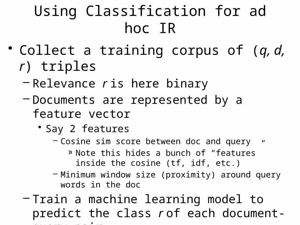
Using Classification for ad hoc IR• Collect a training corpus of (q, d, r) triples

– Relevance r is here binary– Documents are represented by a feature vector

• Say 2 features– Cosine sim score between doc and query

» Note this hides a bunch of “features” inside the cosine (tf, idf, etc.)

– Minimum window size (proximity) around query words in the doc

– Train a machine learning model to predict the class r of each document-query pair• Class is relevant/non-relevant

– Use classifier confidence to generate a ranking

Sec. 15.4.1

Training data

Using classification for ad hoc IR

• A linear scoring function on these two features is then

Score(d, q) = Score(α, ω) = aα + bω + c• And the linear classifier is

Decide relevant if Score(d, q) > θ

Sec. 15.4.1

Using classification for ad hoc IR

02 3 4 5

0.05

0.025

cosi

ne s

core

Term proximity

RR

R

R

R R

R

RR

RR

N

N

N

N

N

N

NN

N

N

Sec. 15.4.1

Decision surfaceDecision surface

10

Linear classifiers: Which Hyperplane?

• Lots of possible solutions for a,b,c.• Some methods find a separating

hyperplane, but not the optimal one – E.g., perceptron

• Support Vector Machine (SVM) finds an optimal solution.– Maximizes the distance between the

hyperplane and the “difficult points” close to decision boundary

– One intuition: if there are no points near the decision surface, then there are no very uncertain classification decisions

This line represents the decision boundary:

ax + by - c = 0

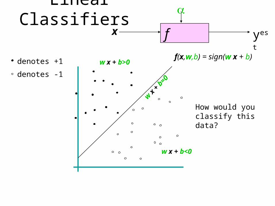
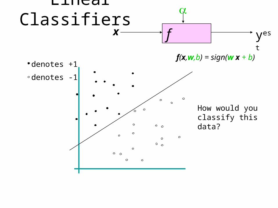
Linear Classifiersf x

a

yest

denotes +1

denotes -1

f(x,w,b) = sign(w x + b)

How would you classify this data?

w x +

b=0

w x + b<0

w x + b>0


a

yest

denotes +1

denotes -1




a

yest

denotes +1

denotes -1




a

yest

denotes +1

denotes -1


Any of these would be fine..

..but which is best?


a

yest

denotes +1

denotes -1



Misclassified to +1 class

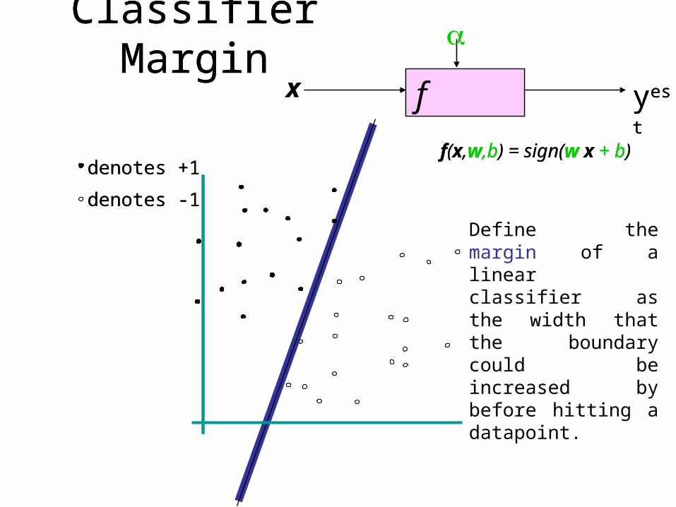
Classifier Marginf x

a

yest

denotes +1

denotes -1


Classifier Marginf x

a

yest

denotes +1

denotes -1


Define the margin of a linear classifier as the width that the boundary could be increased by before hitting a datapoint.

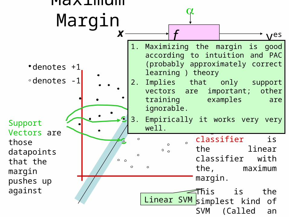
Maximum Marginf x

a

yest

denotes +1

denotes -1


The maximum margin linear classifier is the linear classifier with the, maximum margin.

This is the simplest kind of SVM (Called an LSVM)Linear SVM

Support Vectors are those datapoints that the margin pushes up against

1. Maximizing the margin is good according to intuition and PAC (probably approximately correct learning ) theory

2. Implies that only support vectors are important; other training examples are ignorable.

3. Empirically it works very very well.

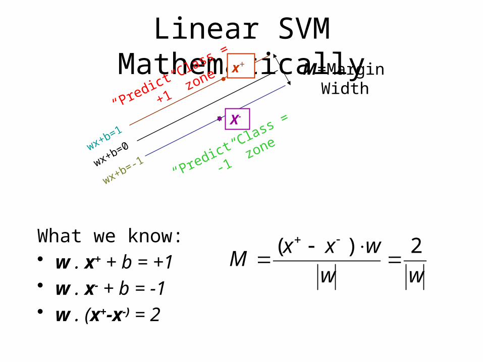
Linear SVM Mathematically

What we know:• w . x+ + b = +1 • w . x- + b = -1 • w . (x+-x-) = 2

“Predict Class

= +1”

zone

“Predict Class

= -1”

zonewx+b=1

wx+b=0

wx+b=-1

X-

x+

ww

wxxM

2)(

M=Margin Width

Support Vector Machine (SVM)Support vectors

Maximizesmargin

• SVMs maximize the margin around the separating hyperplane.

• A.k.a. large margin classifiers

• The decision function is fully specified by a subset of training samples, the support vectors.

• Solving SVMs is a quadratic programming problem

• Seen by many as the most successful current text classification method*

Sec. 15.1

Narrowermargin

wT x + b = 0

wTxa + b = 1

wTxb + b = -1

ρ

WT is the weight vector

r

Linear SVM Mathematically• Assume that all data is at least distance 1 from the hyperplane, then

the following two constraints follow for a training set {(xi ,yi)}

• For support vectors, the inequality becomes an equality• Then, since each example’s distance from the hyperplane is

• The margin is:

wTxi + b ≥ 1 if yi = 1

wTxi + b ≤ -1 if yi = -1

w

2

w

xw byr

T

Sec. 15.1

22

Soft Margin Classification • If the training set is not

linearly separable, slack variables ξi can be added to allow misclassification of difficult or noisy examples.

• Allow some errors– Let some points be

moved to where they belong, at a cost

• Still, try to minimize training set errors, and to place hyperplane “far” from each class (large margin)

ξj

ξi

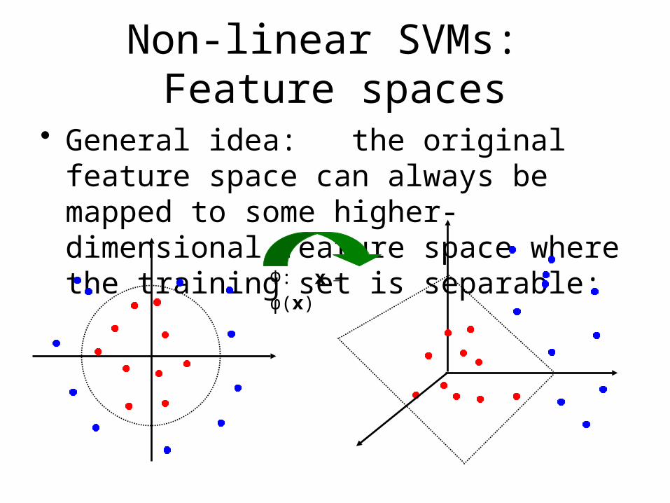
Non-linear SVMs: Feature spaces

• General idea: the original feature space can always be mapped to some higher-dimensional feature space where the training set is separable:

Φ: x → φ(x)

Properties of SVM

• Flexibility in choosing a similarity function• Sparseness of solution when dealing with large data

sets - only support vectors are used to specify the separating

hyperplane • Ability to handle large feature spaces - complexity does not depend on the dimensionality of the

feature space• Overfitting can be controlled by soft margin

approach• Nice math property: a simple convex optimization problem

which is guaranteed to converge to a single global solution• Feature Selection