Machine Learning for

Object RecognitionObject Recognition

Artem Lind & Aleskandr Tkachenko

Outline

• Problem overview

• Classification demo

• Examples of learning algorithms

– Probabilistic modeling– Probabilistic modeling

• Bayes classifier

– Maximum margin classification

• SVM

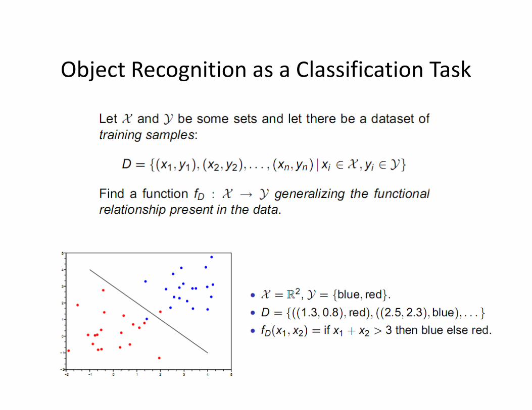
Object Recognition as a Classification Task

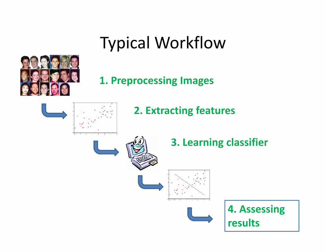
Typical Workflow

2. Extracting features

1. Preprocessing Images

4. Assessing

results

3. Learning classifier

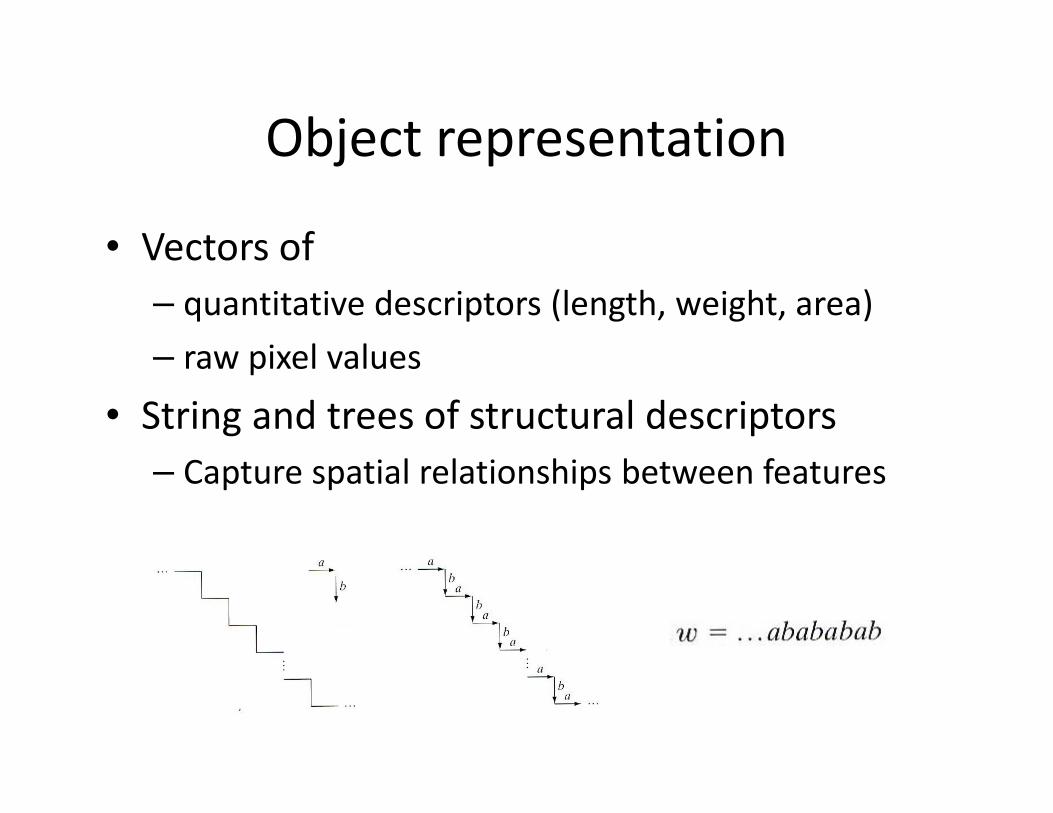
Object representation

• Vectors of

– quantitative descriptors (length, weight, area)

– raw pixel values

• String and trees of structural descriptors• String and trees of structural descriptors

– Capture spatial relationships between features

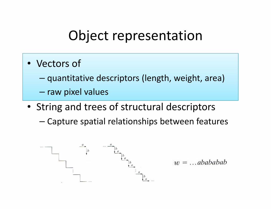
Object representation

• Vectors of

– quantitative descriptors (length, weight, area)

– raw pixel values

• String and trees of structural descriptors• String and trees of structural descriptors

– Capture spatial relationships between features

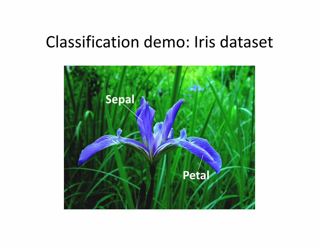
Classification demo: Iris dataset

Sepal

Petal

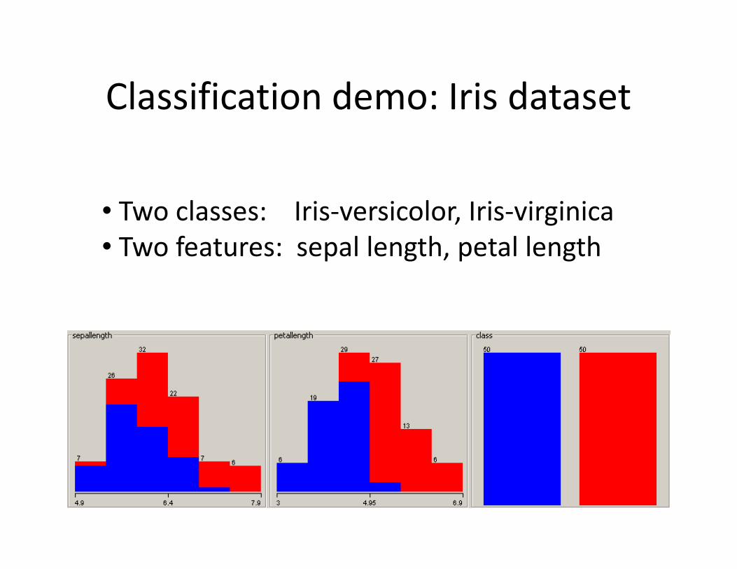
Classification demo: Iris dataset

• Two classes: Iris-versicolor, Iris-virginica

• Two features: sepal length, petal length

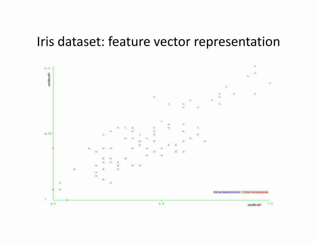
Iris dataset: feature vector representation

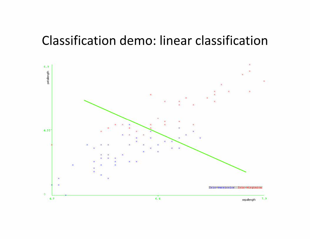
Classification demo: linear classification

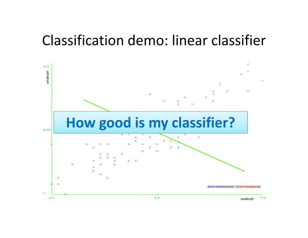
Classification demo: linear classifier

How good is my classifier?How good is my classifier?

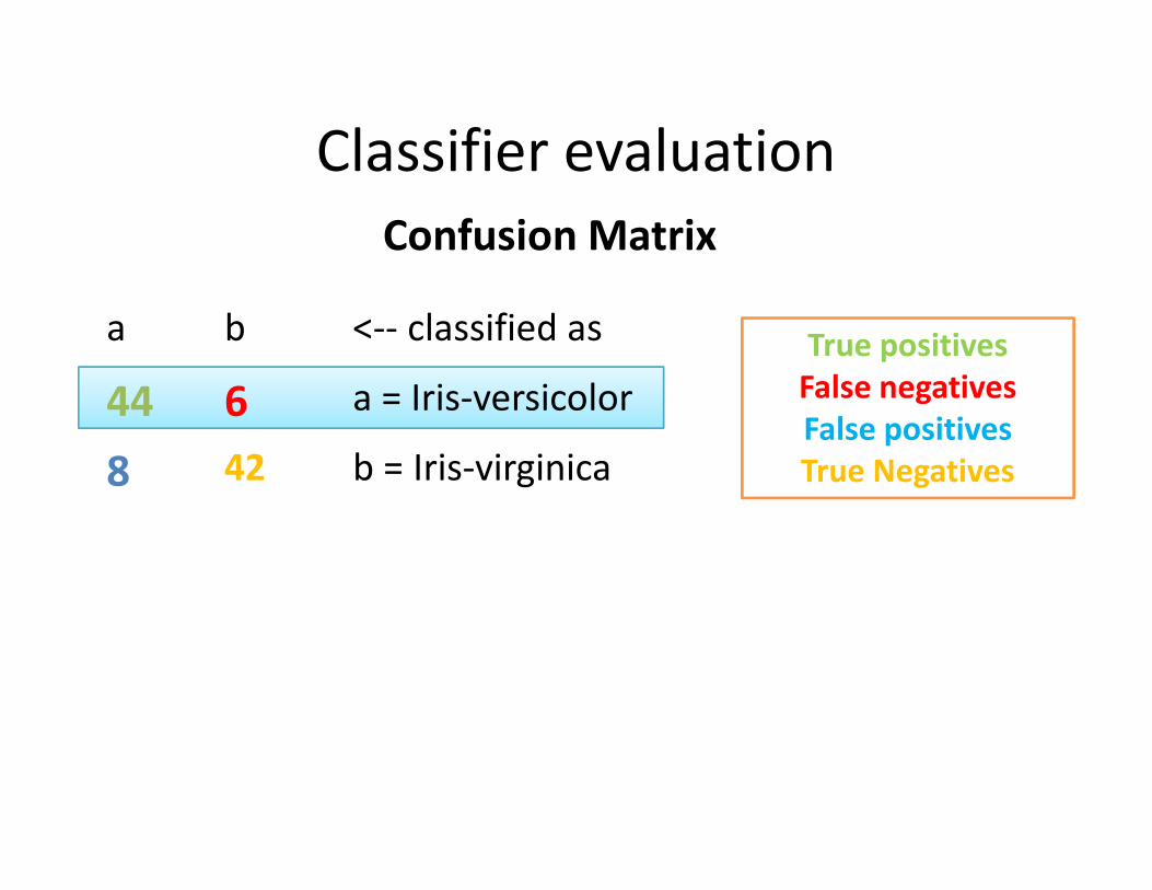
a b <-- classified as

44 6 a = Iris-versicolor

8 42 b = Iris-virginica

Classifier evaluation

Confusion Matrix

True positives

False negatives

False positives

8 42 b = Iris-virginicaFalse positives

True Negatives

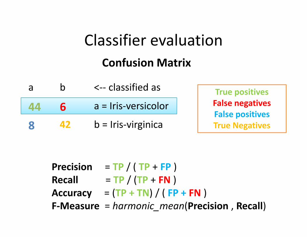
a b <-- classified as

44 6 a = Iris-versicolor

8 42 b = Iris-virginica

Classifier evaluation

Confusion Matrix

True positives

False negatives

False positives

8 42 b = Iris-virginicaFalse positives

True Negatives

Precision = TP / ( TP + FP )

Recall = TP / (TP + FN )

Accuracy = (TP + TN) / ( FP + FN )

F-Measure = harmonic_mean(Precision , Recall)

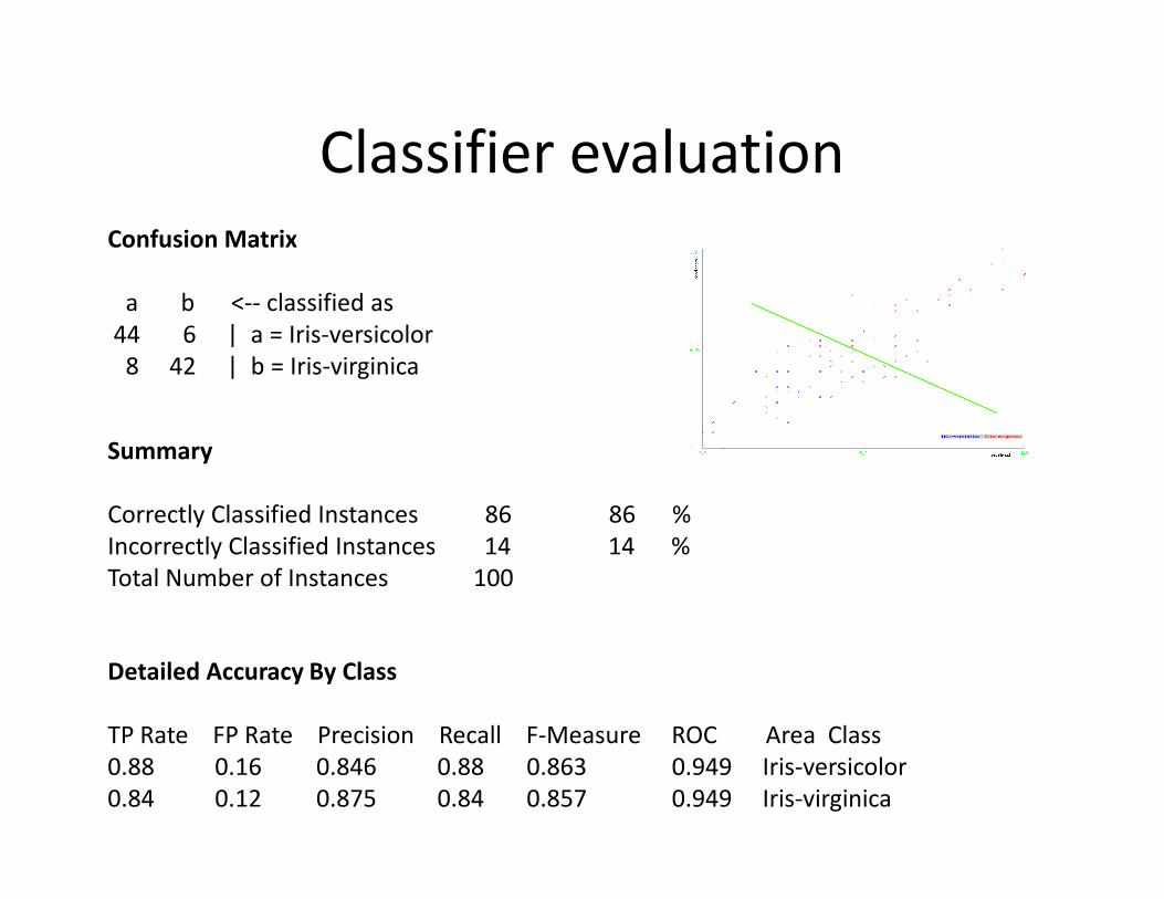
Classifier evaluation

Confusion Matrix

a b <-- classified as

44 6 | a = Iris-versicolor

8 42 | b = Iris-virginica

SummarySummary

Correctly Classified Instances 86 86 %

Incorrectly Classified Instances 14 14 %

Total Number of Instances 100

Detailed Accuracy By Class

TP Rate FP Rate Precision Recall F-Measure ROC Area Class

0.88 0.16 0.846 0.88 0.863 0.949 Iris-versicolor

0.84 0.12 0.875 0.84 0.857 0.949 Iris-virginica

Classifier evaluation

• Most training algorithms optimize Accuracy /

Precision / Recall for the given data

• However, we want classifier to perform well

on “unseen” dataon “unseen” data

– This makes algorithms and theory way more

complicated.

– This makes validation somewhat more

complicated.

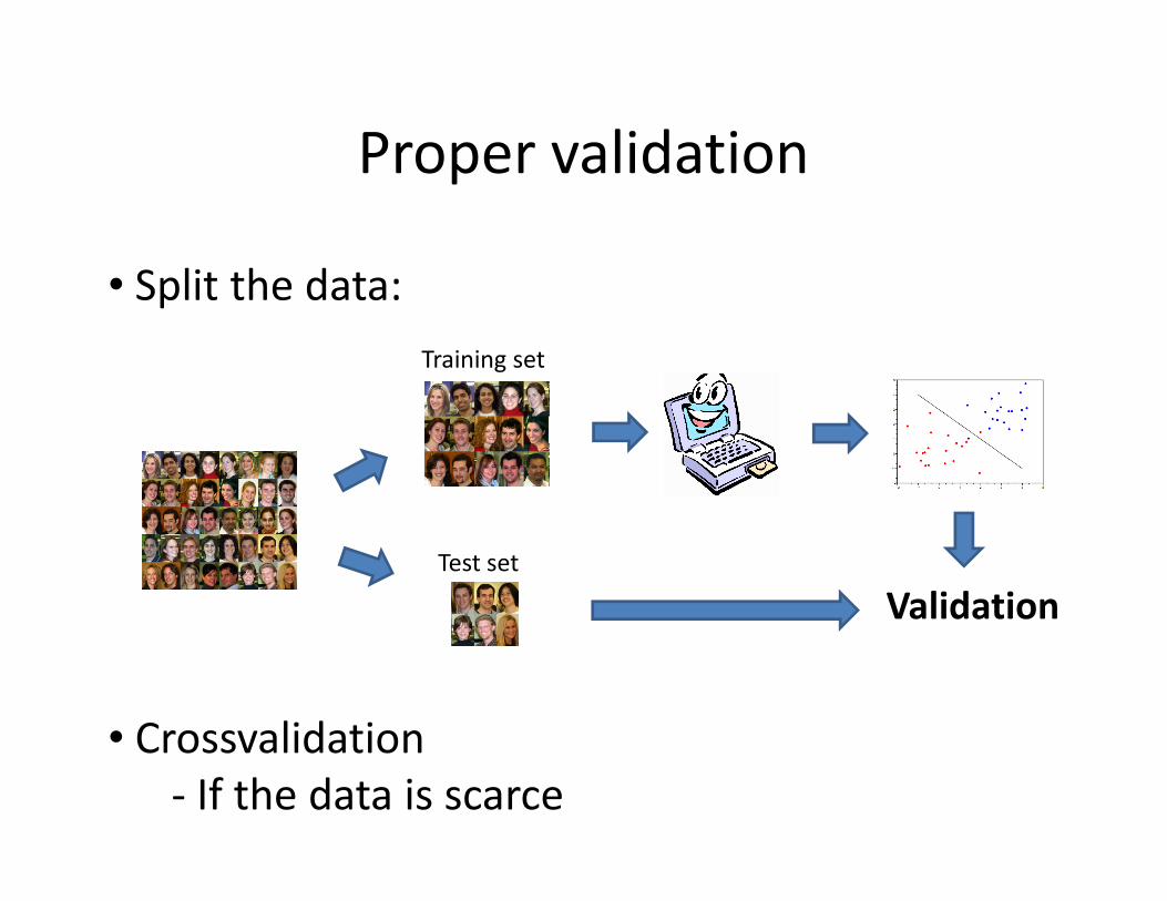
• Split the data:

Proper validation

Training set

• Crossvalidation

- If the data is scarce

Validation

Test set

Common workflow – Summary:

• Get a decent dataset

• Identify discriminative features

• Train your classifier on the training set• Train your classifier on the training set

• Validate on the test set

Classifiers

• Probabilistic modeling

–Bayes classifier

• Margin maximization

–Support Vector Machines

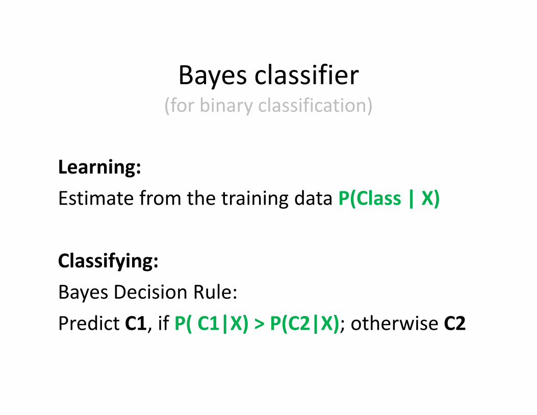
Bayes classifier(for binary classification)

Learning:

Estimate from the training data P(Class | X)Estimate from the training data P(Class | X)

Classifying:

Bayes Decision Rule:

Predict C1, if P( C1|X) > P(C2|X); otherwise C2

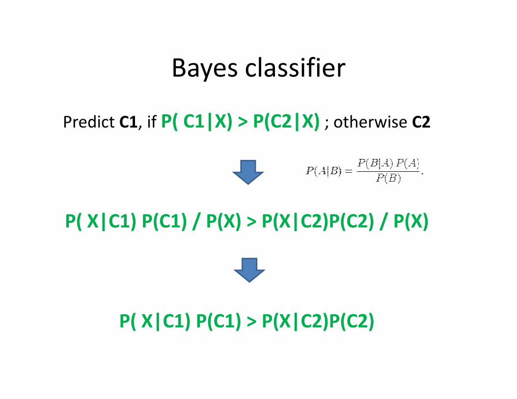
Bayes classifier

Predict C1, if P( C1|X) > P(C2|X) ; otherwise C2

P( X|C1) P(C1) / P(X) > P(X|C2)P(C2) / P(X)

P( X|C1) P(C1) > P(X|C2)P(C2)

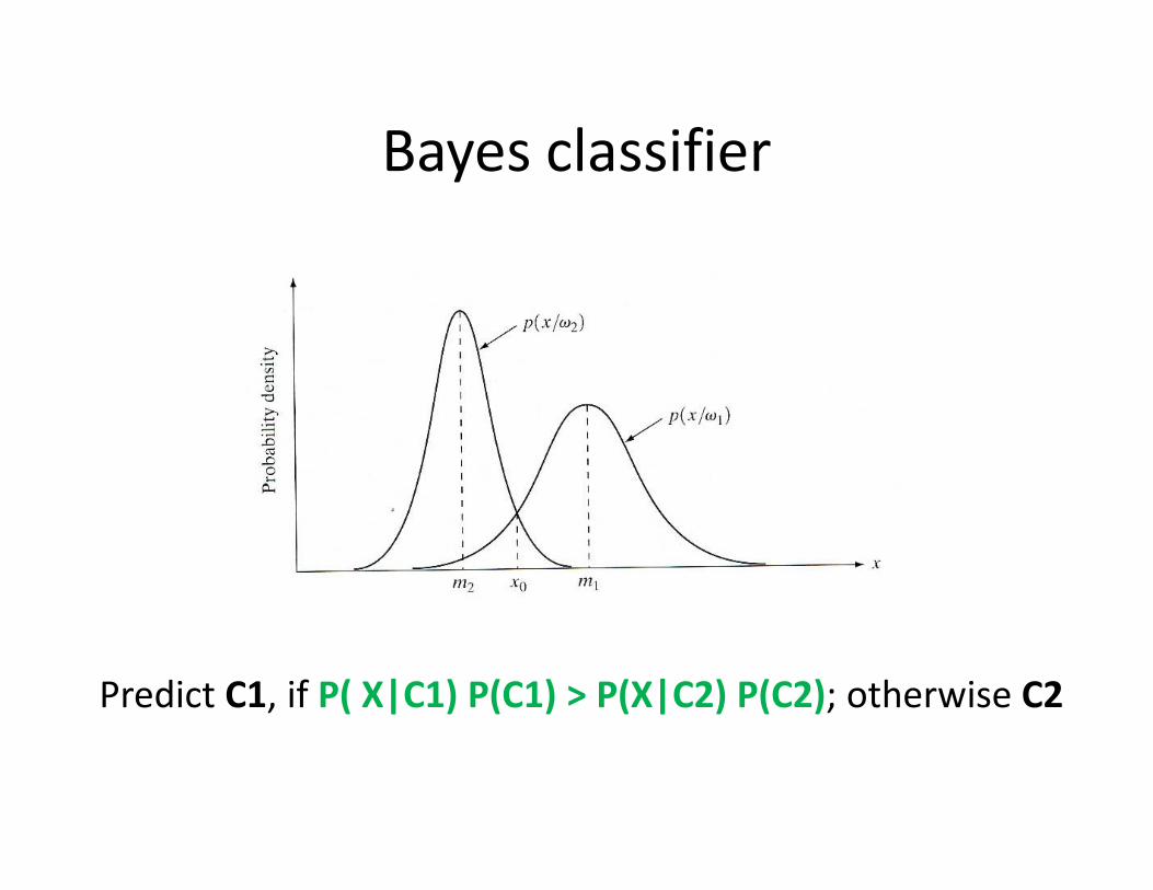
Bayes classifier

Predict C1, if P( X|C1) P(C1) > P(X|C2) P(C2); otherwise C2

Bayes classifier

• If P( X|Class) and P(Class) are known, then the classifier is optimal.

• In practice, distributions P(X|Class) and P(Class) are unknown and need to be estimated from the data:

– P(Class):– P(Class):

• Assign equal probability to all classes

• Use prior knowledge

• P(C) = #examples_in_C / #examples

– P(X | Class):

• Some well-behaved distribution expressed in an analytical form.

• Parameters are estimated based on data for each class.

• The closer this assumption is to reality, the closer the Bayesclassifier approaches the optimum.

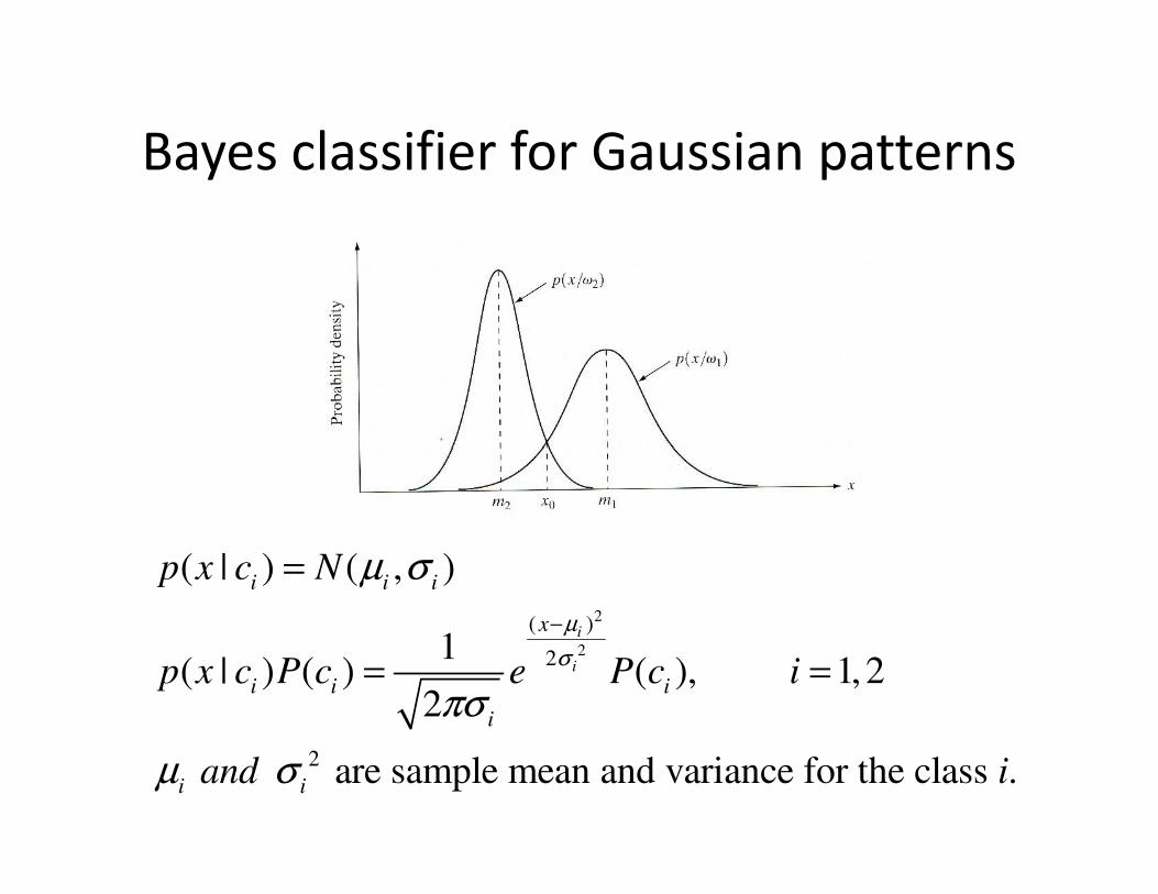
Bayes classifier for Gaussian patterns

2

2

( )

2

2

( | ) ( , )

1( | ) ( ) ( ), 1, 2

2

are sample mean and variance for the class .

i

i

i i i

x

i i i

i

i i

p x c N

p x c P c e P c i

and i

µ

σ

µ σ

πσ

µ σ

−

=

= =

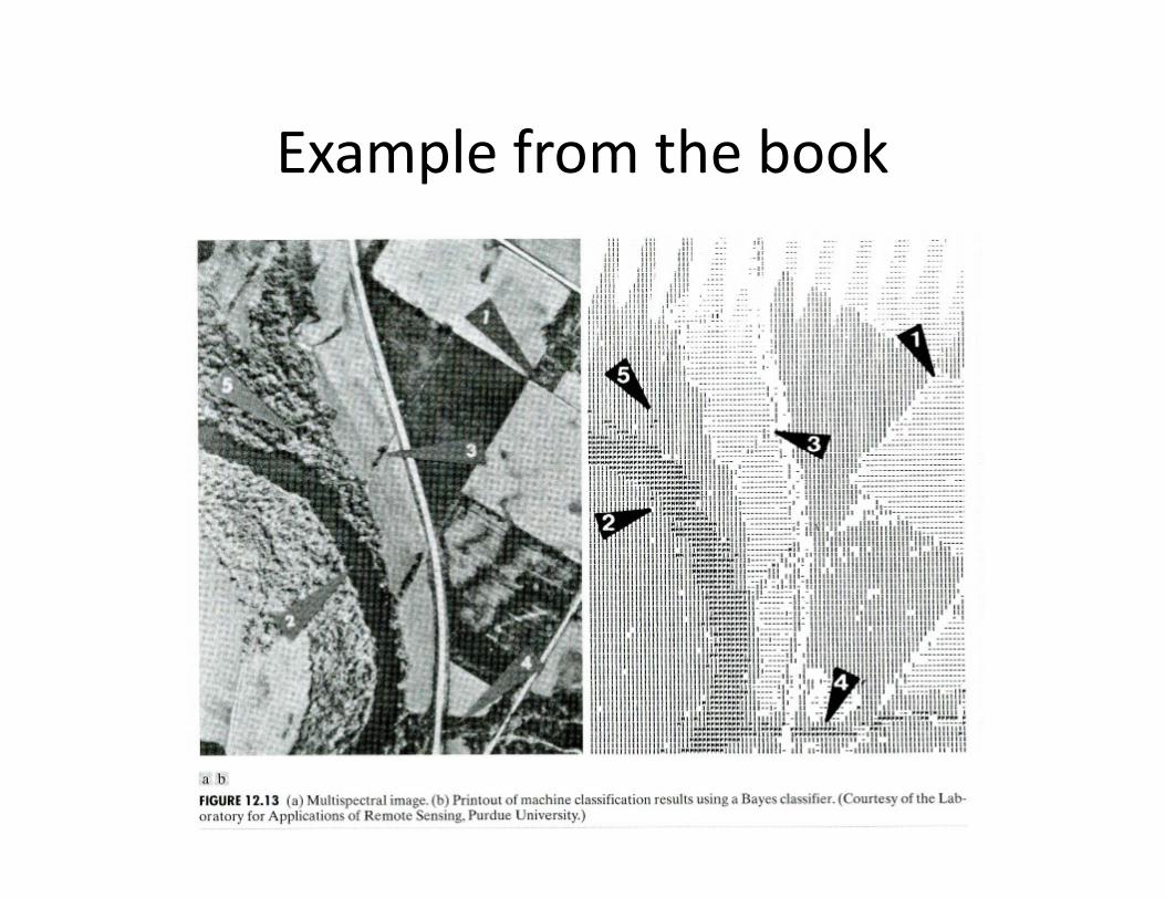
Example from the book

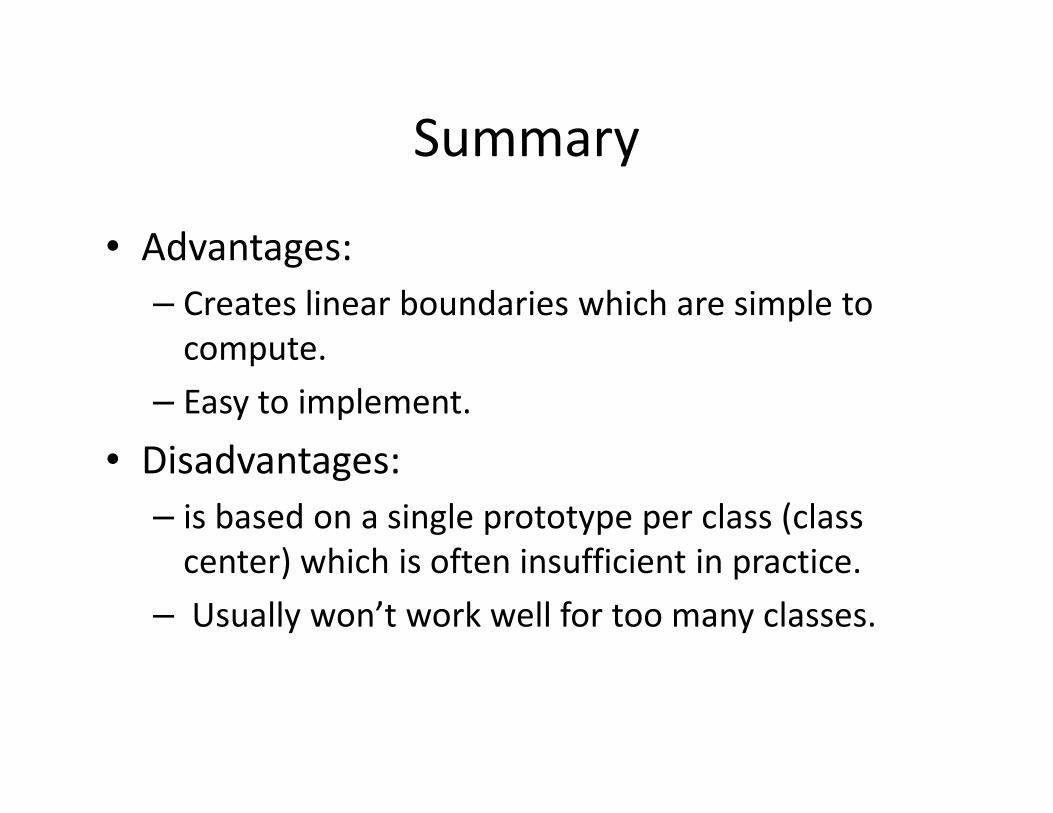
Summary

• Advantages:

– Creates linear boundaries which are simple to

compute.

– Easy to implement.– Easy to implement.

• Disadvantages:

– is based on a single prototype per class (class

center) which is often insufficient in practice.

– Usually won’t work well for too many classes.

Support Vector MachinesSupport Vector Machines

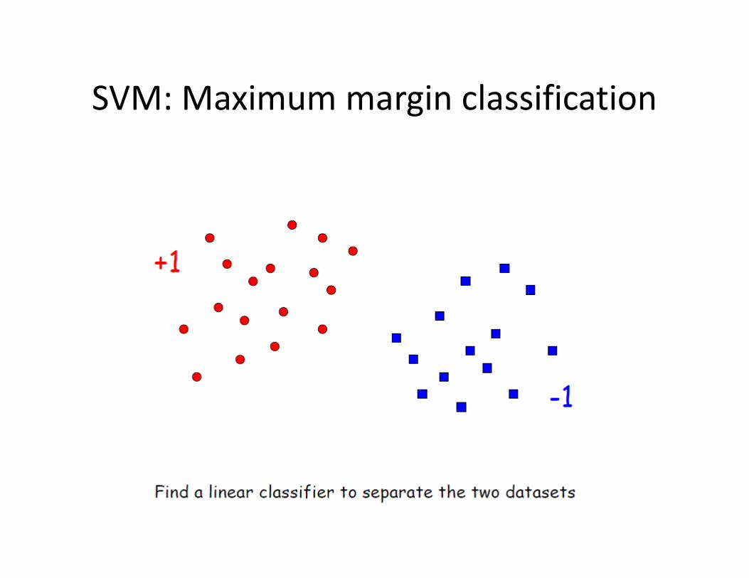
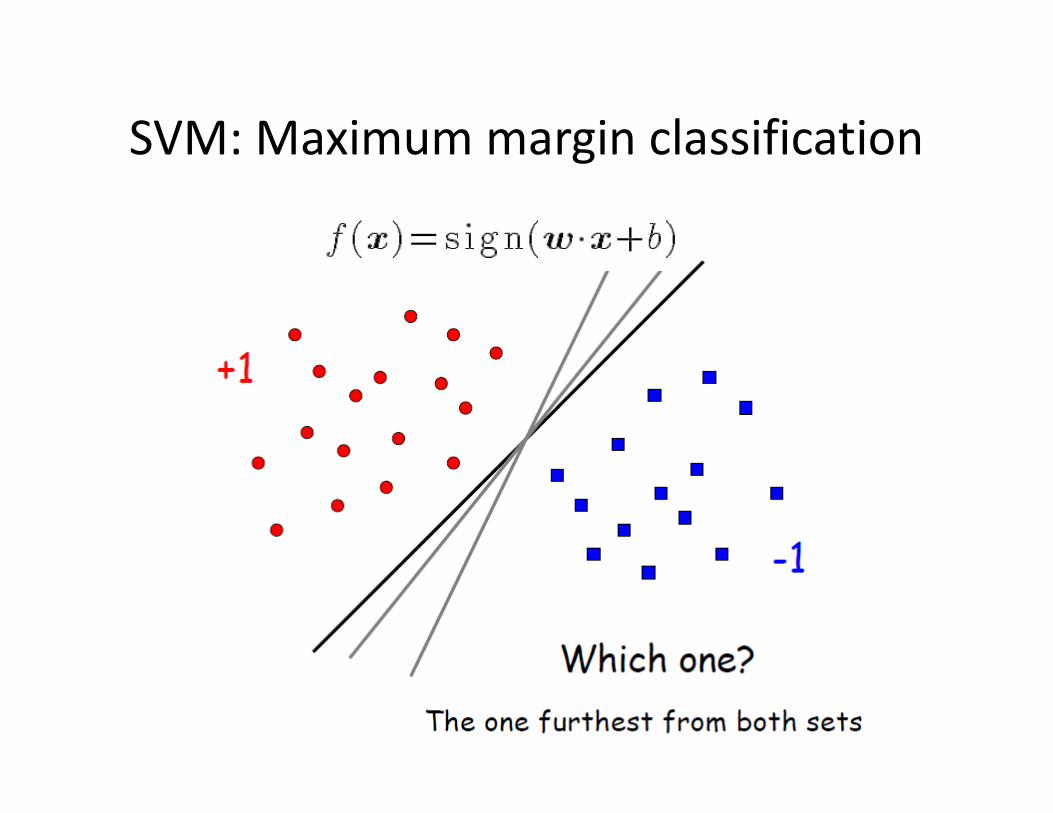
SVM: Maximum margin classification

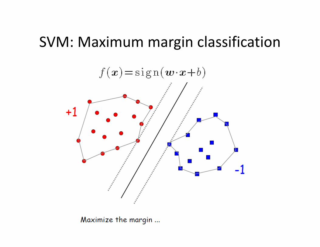
SVM: Maximum margin classification

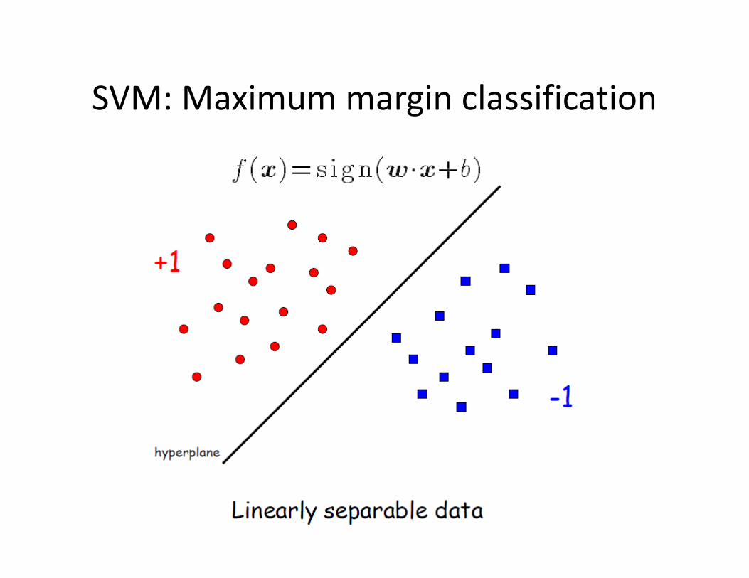
SVM: Maximum margin classification

SVM: Maximum margin classification

SVM: Maximum margin classification

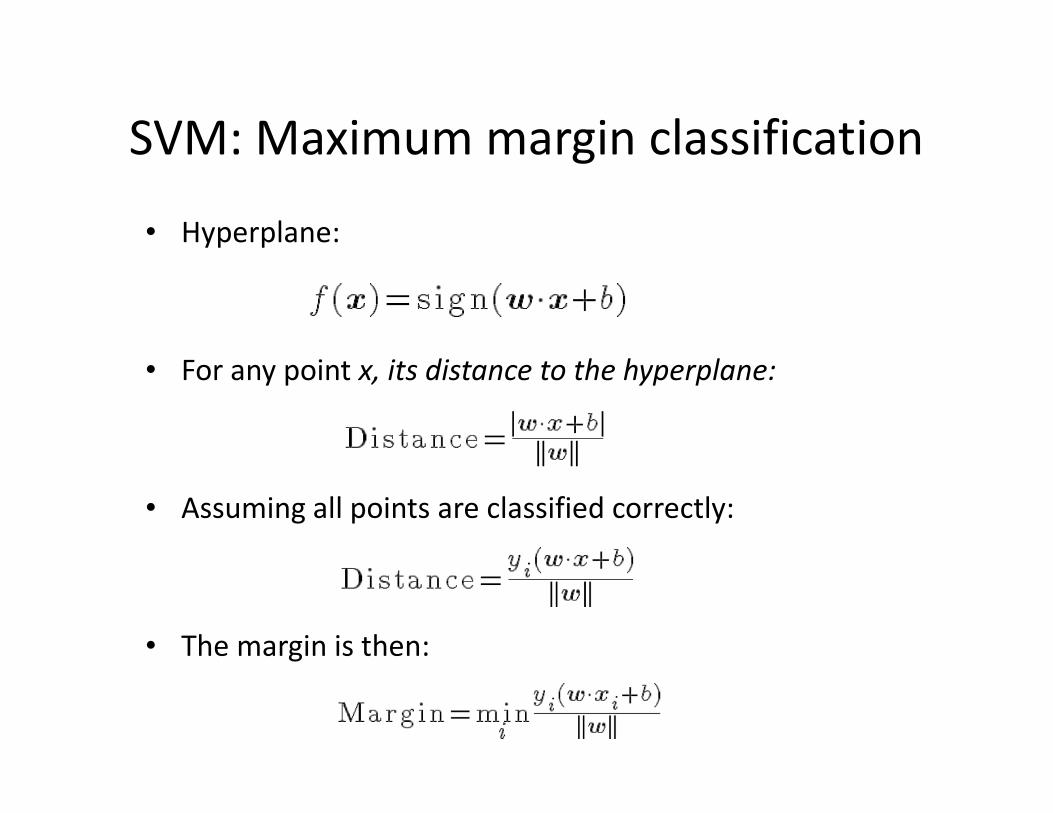
• Hyperplane:

• For any point x, its distance to the hyperplane:

SVM: Maximum margin classification

• Assuming all points are classified correctly:

• The margin is then:

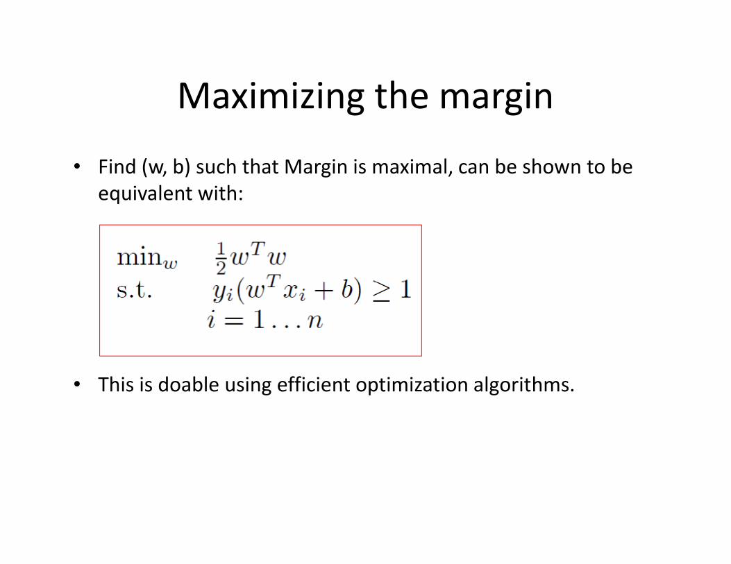
Maximizing the margin

• Find (w, b) such that Margin is maximal, can be shown to be

equivalent with:

• This is doable using efficient optimization algorithms.

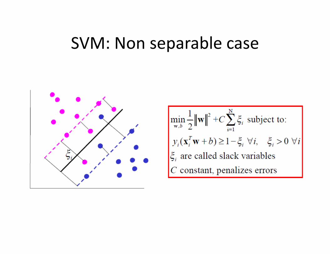
SVM: Non separable case

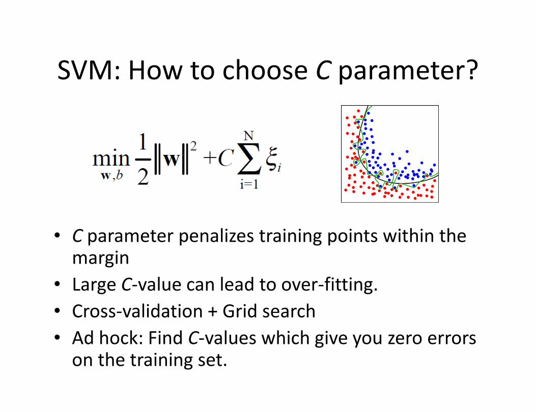
SVM: How to choose C parameter?

• C parameter penalizes training points within the margin

• Large C-value can lead to over-fitting.

• Cross-validation + Grid search

• Ad hock: Find C-values which give you zero errors on the training set.

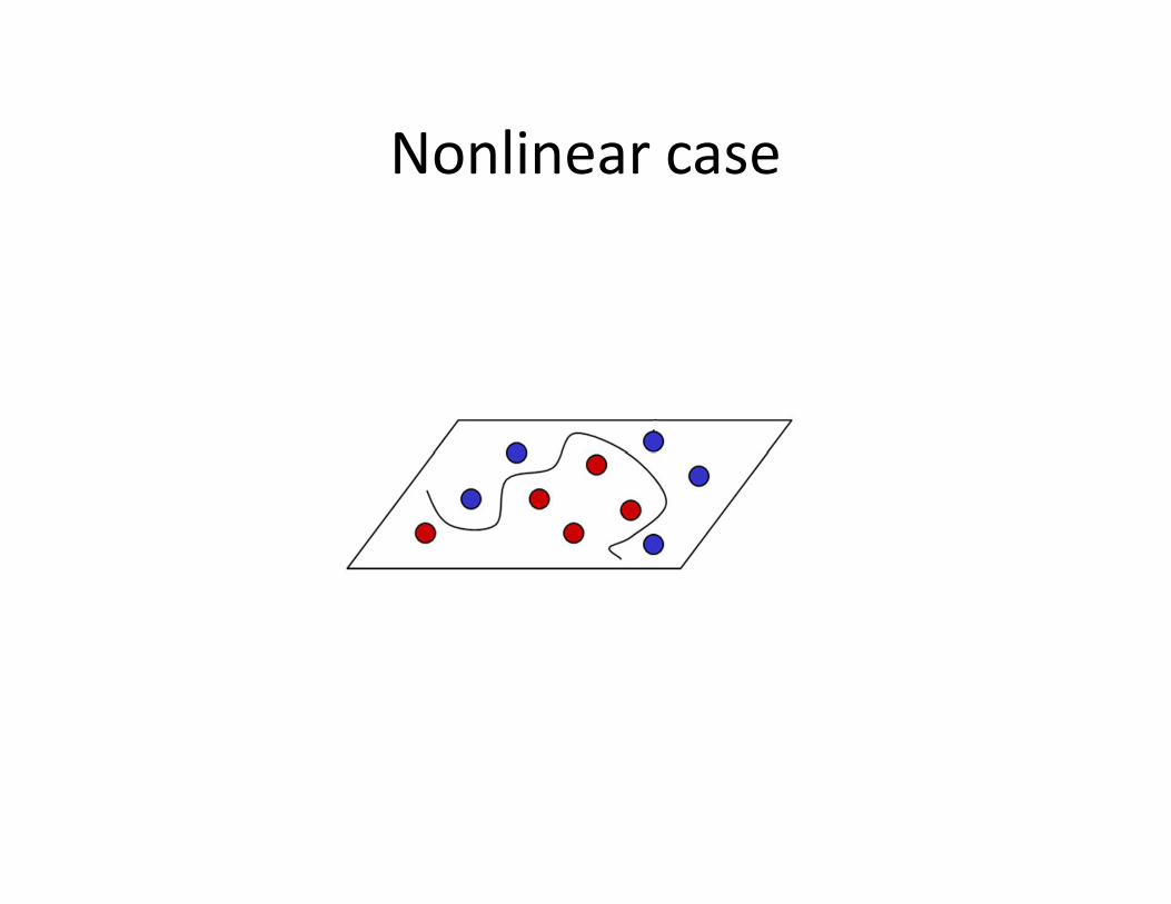
Nonlinear case

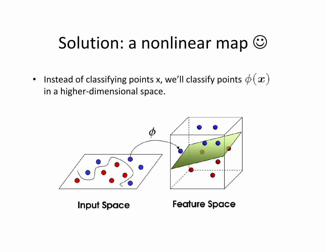
Solution: a nonlinear map ☺

• Instead of classifying points x, we’ll classify points

in a higher-dimensional space.

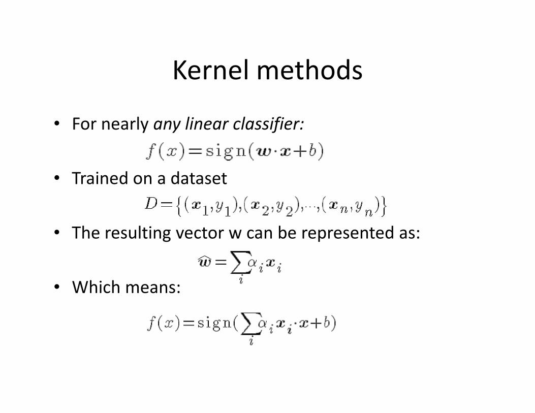
Kernel methods

• For nearly any linear classifier:

• Trained on a dataset

• The resulting vector w can be represented as:

• Which means:

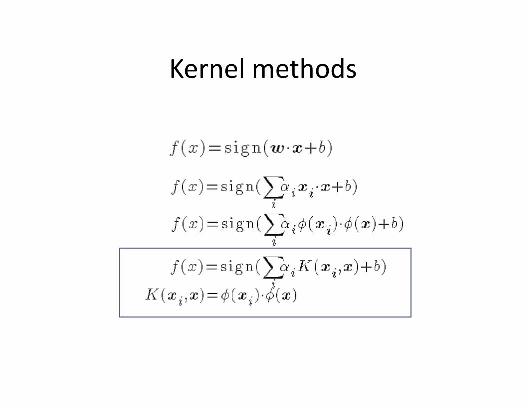
Kernel methods

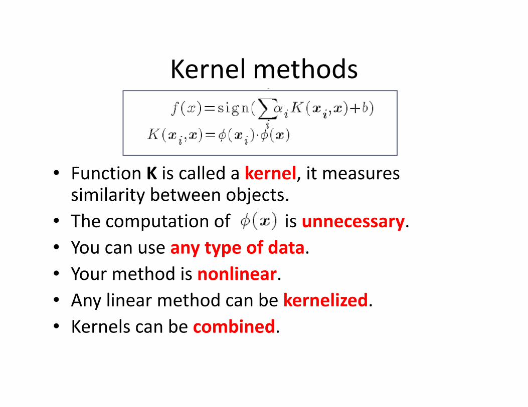
Kernel methods

• Function K is called a kernel, it measures similarity between objects.similarity between objects.

• The computation of is unnecessary.

• You can use any type of data.

• Your method is nonlinear.

• Any linear method can be kernelized.

• Kernels can be combined.

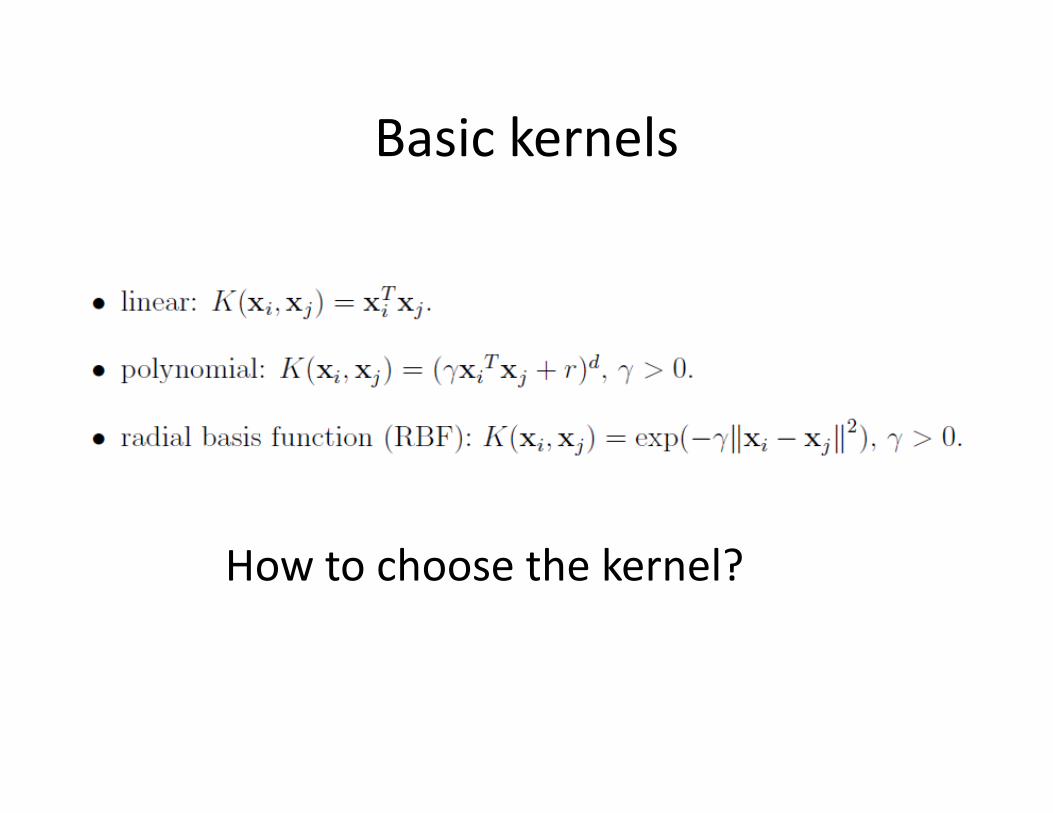
Basic kernels

How to choose the kernel?

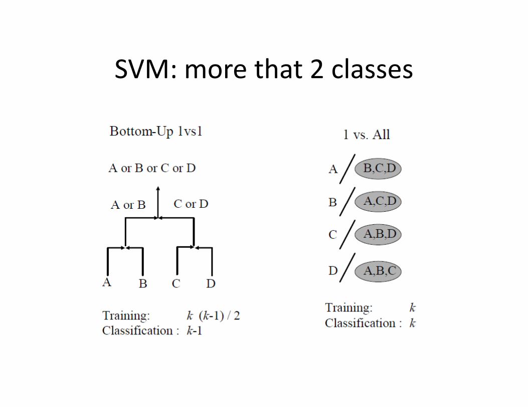
SVM: more that 2 classes

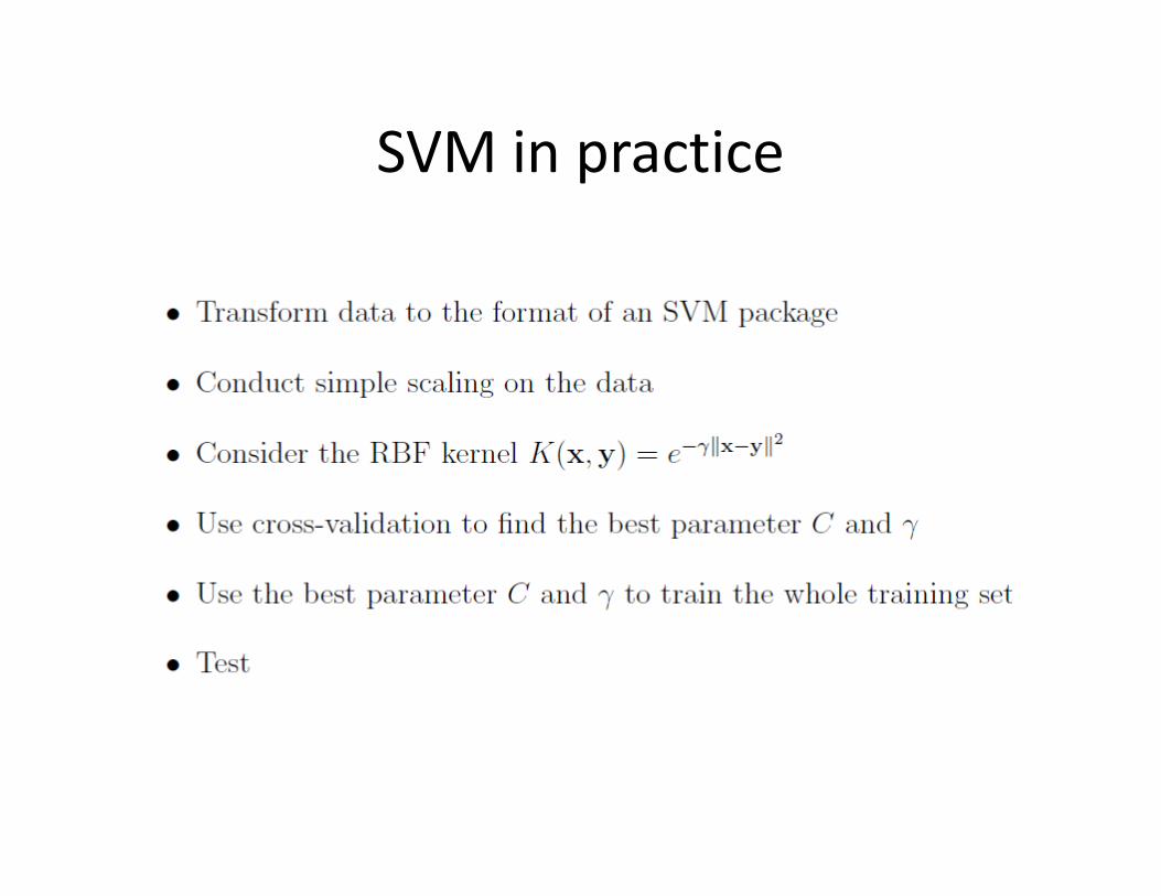
SVM in practice

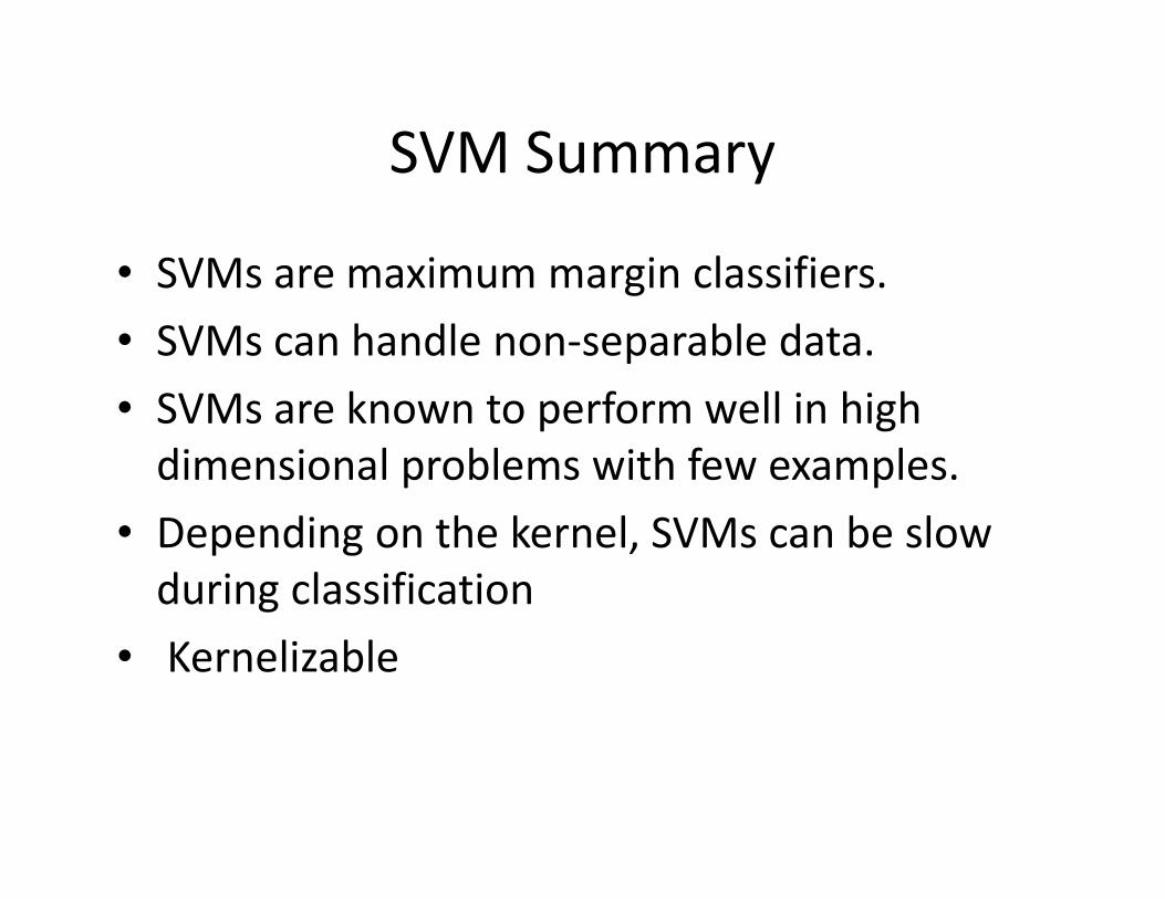
SVM Summary

• SVMs are maximum margin classifiers.

• SVMs can handle non-separable data.

• SVMs are known to perform well in high

dimensional problems with few examples. dimensional problems with few examples.

• Depending on the kernel, SVMs can be slow

during classification

• Kernelizable

References

• Massachusetts Institute of technology course:

– 9.913 Pattern Recognition for Machine Vision

– http://ocw.mit.edu/courses/brain-and-cognitive-sciences/9-913-pattern-recognition-for-machine-vision-fall-2004/fall-2004/

• A Practical Guide to Support Vector Classication

– http://www.csie.ntu.edu.tw/~cjlin/papers/guide/guide.pdf

• Konstantin Tretyakov slides on datamining

– http://courses.cs.ut.ee/2009/dm/Main/Lectures

Demo