Machine Learning for NLPLecture 4: Neural networks

UNIVERSITY OF

GOTHENBURG

Richard Johansson

September 16, 2016

-20pt

UNIVERSITY OF

GOTHENBURG

the �deep learning tsunami�

I in several �elds, such as speech and image processing, neuralnetwork or �deep learning� models have led to dramaticimprovements

I Manning: �2015 seems like the year when the full force of the[deep learning] tsunami hit the major NLP conferences�

I out of the machine learning community: �NLP is kind of like arabbit in the headlights of the deep learning machine, waitingto be �attened�

I so, what's the hype about?

-20pt

UNIVERSITY OF

GOTHENBURG

overview

I neural networks (NNs) are systems that learn to form usefulabstractions automatically

I learn to form larger units from small pieces

I appealing because it can reduce the feature engineering e�ortI image borrowed from Josephine Sullivan:

I NNs are excellent for �noisy� problems such as speech andimage processing

I while powerful, they can be cumbersome to train and tend torequire quite a bit of tweaking

-20pt

UNIVERSITY OF

GOTHENBURG

causes of the NN resurgence

I NNs seem to have a hype cycle of about 20 yearsI there are a number of reasons for the one we're currently inI the most important is increasing computational capacity

I for instance, the famous �cat paper� by Stanford/Googlerequired 1,000 machines (16,000 CPUs)

I Le et al: Building high-level features using large scale

unsupervised learning, ICML 2011.

I much of the recent research is coming out of Google(DeepMind), Microsoft, Facebook, etc.

I using GPUs from graphics cards can speed up training

I also, a number of new methods proposed recently

-20pt

UNIVERSITY OF

GOTHENBURG

overview

I today: NNs for classi�cationI Monday: NNs for sequences (e.g. tagging, translation)

-20pt

UNIVERSITY OF

GOTHENBURG

overview

basic ideas in neural network classi�ers

overview of neural network libraries

word embeddings and distributional semantics

-20pt

UNIVERSITY OF

GOTHENBURG

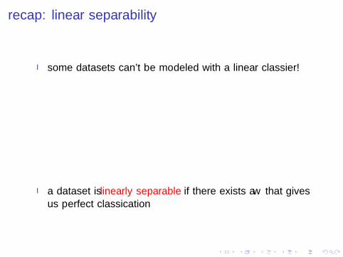
recap: linear separability

I some datasets can't be modeled with a linear classi�er!

I a dataset is linearly separable if there exists a w that givesus perfect classi�cation

-20pt

UNIVERSITY OF

GOTHENBURG

example: XOR dataset

X = numpy.array([[1, 1],

[1, 0],

[0, 1],

[0, 0]])

Y = ['no', 'yes', 'yes', 'no']

clf = LinearSVC()

clf.fit(X, Y)

# linear inseparability, so we get less than 100% accuracy

print(accuracy_score(Y, clf.predict(X)))

-20pt

UNIVERSITY OF

GOTHENBURG

�abstraction� by forming feature combinations

I recall from a previout lecture that we can add �usefulcombinations� of features to make the dataset separable:

very good very-good Positivevery bad very-bad Negativenot good not-good Negativenot bad not-bad Positive

-20pt

UNIVERSITY OF

GOTHENBURG

example: XOR dataset with a combination feature

# feature1, feature2, feature1&feature2

X = numpy.array([[1, 1, 1],

[1, 0, 0],

[0, 1, 0],

[0, 0, 0]])

Y = ['no', 'yes', 'yes', 'no']

clf = LinearSVC()

clf.fit(X, Y)

# now we have linear separability, so we get 100%

print(accuracy_score(Y, clf.predict(X)))

-20pt

UNIVERSITY OF

GOTHENBURG

expressing feature combinations as �sub-classi�ers�

I instead of de�ning a rule, such as x3 = x1 AND x2, we couldimagine that the combination feature x3 would be computedby a separate classi�er, for instance LR

I we could train a classi�er using the output of �sub-classi�ers�

-20pt

UNIVERSITY OF

GOTHENBURG

�neurons�

I historically, NNs were inspired byhow biological neural systemswork � hence the name

I as far as I know, modern NNsand modern neuroscience don'thave much in common

I Andrew Ng: �A single neuron in the brain is an incredibly complex

machine that even today we don't understand. A single `neuron' in

a neural network is an incredibly simple mathematical function that

captures a minuscule fraction of the complexity of a biological

neuron. So to say neural networks mimic the brain, that is true at

the level of loose inspiration, but really arti�cial neural networks are

nothing like what the biological brain does.�

-20pt

UNIVERSITY OF

GOTHENBURG

recap: the logistic or sigmoid function

def logistic(scores):

return 1 / (1 + numpy.exp(-scores))

-20pt

UNIVERSITY OF

GOTHENBURG

a multilayered classi�er

I a feedforward neural network or multilayer perceptronconsists of connected layers of �classi�ers�

I the intermediate classi�ers are called hidden unitsI the �nal classi�er is called the output unit

I let's assume two layers for nowI each hidden unit hi computes its output based on its own

weight vector whi:

hi = f (whi· x)

I and then the output is computed from the hidden units:

y = f (wo · h)

I the function f is called the activationI in this lecture, we'll assume that f is the logistic function, so

the hidden units and output unit can be seen as LR classi�ers

-20pt

UNIVERSITY OF

GOTHENBURG

two-layered feedforward NN: �gure

-20pt

UNIVERSITY OF

GOTHENBURG

implementation in NumPy

I recall that a sequence of dot products can be seen as a matrixmultiplication

I in NumPy, the NN can be expressed compactly with matrixmultiplication

h = logistic(Wh.dot(x))

y = logistic(Wo.dot(h))

-20pt

UNIVERSITY OF

GOTHENBURG

expressivity of feedforward NNs

I Hornik's universal approximation theorem shows thatfeedforward NNs can approximate any (bounded)mathematical function

I Hornik (1991). Approximation capabilities of multilayer

feedforward networks. Neural Networks, 4(2), 251�257.

I and this is true even with a single hidden layer!

I however, this is mainly of theoretical interestI the theorem does not say how many hidden units we needI and it doesn't say how the network should be trained

-20pt

UNIVERSITY OF

GOTHENBURG

expressivity of feedforward NNs

I Hornik's universal approximation theorem shows thatfeedforward NNs can approximate any (bounded)mathematical function

I Hornik (1991). Approximation capabilities of multilayer

feedforward networks. Neural Networks, 4(2), 251�257.

I and this is true even with a single hidden layer!I however, this is mainly of theoretical interest

I the theorem does not say how many hidden units we needI and it doesn't say how the network should be trained

-20pt

UNIVERSITY OF

GOTHENBURG

�deep learning�

I why the �deep� in �deep learning�?I although a single hidden layer is su�cient in theory, in practice

it can be better to have several hidden layers

-20pt

UNIVERSITY OF

GOTHENBURG

training feedforward neural networks

I training a NN consists of �nding the weights in the layersI so how do we �nd those weights?

I exactly as we did for the SVM and LR!I state an objective function with a loss

I log loss, hinge loss, etc

I and then tweak the weights to make that loss smallI again, we can use (stochastic) gradient descent to minimize

the loss

-20pt

UNIVERSITY OF

GOTHENBURG

training feedforward neural networks

I training a NN consists of �nding the weights in the layersI so how do we �nd those weights?I exactly as we did for the SVM and LR!I state an objective function with a loss

I log loss, hinge loss, etc

I and then tweak the weights to make that loss smallI again, we can use (stochastic) gradient descent to minimize

the loss

-20pt

UNIVERSITY OF

GOTHENBURG

example

I let's use two layers with logistic units, and then the logloss

h = σ(W h · x)y = σ(W o · h)loss = − log(y)

I so the whole thing becomes

loss = − log σ(W o · σ(W h · x))I now, to do gradient descent, we need to compute gradients

w.r.t. the weights W h and W o

I ouch! it looks completely unwieldy!

-20pt

UNIVERSITY OF

GOTHENBURG

example

I let's use two layers with logistic units, and then the logloss

h = σ(W h · x)y = σ(W o · h)loss = − log(y)

I so the whole thing becomes

loss = − log σ(W o · σ(W h · x))I now, to do gradient descent, we need to compute gradients

w.r.t. the weights W h and W o

I ouch! it looks completely unwieldy!

-20pt

UNIVERSITY OF

GOTHENBURG

the chain rule of derivatives/gradients

I NNs consist of functions applied to the output of otherfunctions

I the chain rule is a useful trick from calculus that can be usedin such situations

I assume that we apply the function f to the output of gI then the chain rule says how we can compute the gradient of

the combination:

gradient of f (g(x)) = gradient of f (g) · gradient of g(x)

-20pt

UNIVERSITY OF

GOTHENBURG

the general recipe: backpropagation

I using the chain rule, the gradients of the weights in eachlayer can be computed from the gradients of the layersafter it

I this trick is called backpropagation

I it's not di�cult, but involves a lot of book-keepingI fortunately, there are computer programs that can do the

algebra for us!I in NN software, we usually just declare the network and

the loss, then the gradients are computed under the hood

-20pt

UNIVERSITY OF

GOTHENBURG

optimizing NNs

I unlike the linear classi�ers we studied previously, NNs havenon-convex objective functions with a lot of local minima

I so the end result depends on initialization

−3 −2 −1 0 1 2−3

−2

−1

0

1

2

0.150

0.150

0.300

0.300

0.450

0.450

0.600

0.600

0.750

0.900

-20pt

UNIVERSITY OF

GOTHENBURG

training e�ciency of NNs

I our previous classi�ers took seconds or minutes to trainI NNs tend to take minutes, hours, days, weeks . . .

I depending on the complexity of the network and the amount oftraining data

I NNs use a lot of linear algebra (matrix multiplications) so itcan be useful to work to speed up the math

I parallelize as much as possibleI use optimized math librariesI use a GPU

-20pt

UNIVERSITY OF

GOTHENBURG

overview

basic ideas in neural network classi�ers

overview of neural network libraries

word embeddings and distributional semantics

-20pt

UNIVERSITY OF

GOTHENBURG

neural network software: Python

I scikit-learn currently has very limited support for NNsI the main NN software in the Python world used to be Theano

I developed by Yoshua Bengio's group in MontréalI http://deeplearning.net/software/theano

I last year, Google released their NN library called TensorFlowI https://www.tensorflow.org

-20pt

UNIVERSITY OF

GOTHENBURG

neural network software: Python (2)

I Theano and TensorFlow do a lot of useful math stu�, andintegrates nicely with the GPU, but they can be a bit low-level

I so there are a few libraries that package Theano or TensorFlowin a more user-friendly way, similar to scikit-learn

I Keras: https://github.com/fchollet/kerasI sk�ow: now included in TensorFlow

-20pt

UNIVERSITY OF

GOTHENBURG

other neural network software

I Ca�e: http://caffe.berkeleyvision.org/I Torch: http://torch.ch/

-20pt

UNIVERSITY OF

GOTHENBURG

coding example with Keras

keras_model = Sequential()

n_hidden = 3

keras_model.add(Dense(input_dim=X.shape[1],

output_dim=n_hidden))

keras_model.add(Activation("sigmoid"))

keras_model.add(Dense(input_dim=n_hidden,

output_dim=1))

keras_model.add(Activation("sigmoid"))

keras_model.compile(loss='binary_crossentropy',

optimizer='rmsprop')

keras_model.fit(X, Y)

-20pt

UNIVERSITY OF

GOTHENBURG

coding example with (high-level) TensorFlow

cols = [real_valued_column("", dimension=2)]

classifier = DNNClassifier(feature_columns=cols,

hidden_units=[3],

n_classes=2,

model_dir="/tmp/tftest_model")

classifier.fit(x=X, y=Y)

-20pt

UNIVERSITY OF

GOTHENBURG

overview

basic ideas in neural network classi�ers

overview of neural network libraries

word embeddings and distributional semantics

-20pt

UNIVERSITY OF

GOTHENBURG

representing words in NNs

I NN implementations tend to prefer dense vectorsI this can be a problem if we are using word-based featuresI recall the way we code word features as sparse vectors:

tomato → [0, 0, 1, 0, 0, . . . , 0, 0, 0]carrot → [0, 0, 0, 0, 0, . . . , 0, 1, 0]

I the solution: represent words with low-dimensional vectors, ina way so that words with similar meaning have similar vectors

tomato → [0.10,−0.20, 0.45, 1.2,−0.92, 0.71, 0.05]carrot → [0.08,−0.21, 0.38, 1.3,−0.91, 0.82, 0.09]

I in the NN community, the word vectors are called embeddings

-20pt

UNIVERSITY OF

GOTHENBURG

discovering �meaning� automatically

I there's a growing interest in methods that pick up some sort ofword meaning simply by observing raw text

I these methods require large amounts of text but little or noinvestment in �knowledge engineering�

I you can go home after this talk and try out the software I'llmention, while building an ontology would take you years

I text is cheap nowadays

-20pt

UNIVERSITY OF

GOTHENBURG

vector space models of lexical meaning

I in a word vector space, the �meaning� of a word isrepresented as a vector

pizzasushi

falafel

spaghetti

rock

techno

funksoul

punkjazz

routertouchpad

laptop

monitor

I the spaces typically have 50�10,000 dimensions, but we show2D here for practical reasons

-20pt

UNIVERSITY OF

GOTHENBURG

distances/similarities in a word space

I in a word space, �similarity� of words corresponds to geometryI being near each other in the spaceI . . . or pointing in a similar direction

I pizza is kind of like sushi, but not so much like touchpad

I on the other hand, it seems that we have lost the knowledgestructure: we don't know how pizza and sushi are similar

-20pt

UNIVERSITY OF

GOTHENBURG

how could this work? the distributional hypothesis

I �you shall know a word by the company it keeps�[Firth, 1957]

I two words probably have a similar �meaning� if they tendto appear in similar contexts

I the distributional hypothesis: the distribution ofcontexts in which a word appears is a good proxy of themeaning of that word

I this is the �weak� DH: we use the distribution as apractical representation of meaning because we think itcan be useful

I the �strong� DH on the other hand claims that this is animportant mechanism for concept-formation [Lenci, 2008]

-20pt

UNIVERSITY OF

GOTHENBURG

so what are contexts?

I two words probably mean about the same thing if theyI . . . appear in the same documents?I . . . tend to have the same words around them?I . . . are illustrated with similar images?

-20pt

UNIVERSITY OF

GOTHENBURG

example: most frequent verbs near cake and pizza

I what are the activities we do with cakes and pizzas?I cake: eat, bake, throw, cut, buy, get, decorate, garnish,

make, serve, orderI pizza: eat, bake, order, munch, buy, serve, garnish, name,

get, make, heat

-20pt

UNIVERSITY OF

GOTHENBURG

example: tårta and pizza in Swedish text

-20pt

UNIVERSITY OF

GOTHENBURG

the context is the document

D1: The stock market crashed in Tokyo.D2: Cook the lentils gently in butter.

D1 D2stock 1 0market 1 0crashed 1 0Tokyo 1 0cook 0 1lentils 0 1gently 0 1butter 0 1

I for instance [Landauer and Dumais, 1997]

-20pt

UNIVERSITY OF

GOTHENBURG

using a context based on syntax

has subject I has object book has object bananaread 1 1 0wrote 1 1 0

I for instance[Padó and Lapata, 2007, Levy and Goldberg, 2014a]

-20pt

UNIVERSITY OF

GOTHENBURG

using a multimodal context

The black cat stared at me.

black stared bananacat 1 1 0 1 1 0

I for instance [Lazaridou et al., 2015]

-20pt

UNIVERSITY OF

GOTHENBURG

similarity of meaning vectors

I given two word meaning vectors, we can apply a similarity ordistance function

I Euclidean distance: multidimensional equivalent of ourintuitive notion of distance

I it is 0 if the vectors are identical

I cosine similarity: multiply the coordinates, divide by thelengths

I it is 1 if the vectors are identical, 0 if completely di�erent

I . . . and a whole bunch of other similarities and distances: seeJ&M or one of the survey articles

-20pt

UNIVERSITY OF

GOTHENBURG

example: the nearest neighbors of Berlin

I simple vector space just counting the words before and afterI computed using a subset of EuroparlI the nearest neighbors according to the cosine similarity:

0.933 Cairo

0.925 Johannesburg

0.925 Stockholm

0.924 Madrid

0.922 Bonn

0.919 Abuja

0.918 Thessaloniki

0.917 Helsinki

0.917 Seville

0.915 Tokyo

0.913 Gothenburg

-20pt

UNIVERSITY OF

GOTHENBURG

example: di�erent types of context (cosine similarity)

Reinfeldt: 1

Skavlan: 0.897105

Ludl: 0.878873

Lindson: 0.874008

Gertten: 0.871961

Stillman: 0.871375

Adolph: 0.86191

Ritterberg: 0.852531

Böök: 0.848459

Kessiakoff: 0.834909

Strage: 0.82995

Rinaldo: 0.825585

Reinfeldt: 1

Bildt: 0.973508

Sahlin: 0.960694

rödgröna: 0.960072

Reinfeldts: 0.958742

Juholt: 0.958644

uttalade: 0.956048

rådet: 0.954971

statsministern: 0.952898

politiker: 0.952712

Odell: 0.952376

Schyman: 0.952065

-20pt

UNIVERSITY OF

GOTHENBURG

weighting the context counts

I the useful signal may be drowned out by general function wordsI we can use an association measure (e.g. the PMI) to amplify

the relative importance of the useful contexts

city �sh borsch and theGothenburg 26 14 0 450 675Moscow 31 2 12 389 712

⇓

city �sh borsch and theGothenburg 8.5 9.8 0 0.01 0.005Moscow 8.7 0.5 7.6 0.008 0.006

-20pt

UNIVERSITY OF

GOTHENBURG

dealing with high-dimensional vectors

I typically, there are many possible contexts, so thedistributional vectors will have a high dimensionality

I so they are costly to process in terms of time and memory

I dimensionality reduction: an operation that transforms ahigh-dimensional matrix into a lower-dimensional one

I for instance: 1 million → 100

I the idea of the dimensionality reduction is to �ndlower-dimensional vectors that approximately preserve thedistances between the higher-dimensional vectors

I dimensions no longer interpretable!

-20pt

UNIVERSITY OF

GOTHENBURG

examples of dimensionality reduction methods

I the popular Latent Semantic Analysis (LSA)[Landauer and Dumais, 1997] uses a matrix operation calledsingular value decomposition

I random projection [Kanerva et al., 2000] is a very e�cientalternative to advanced matrix operations: see for instance thePhD thesis by [Sahlgren, 2006]

-20pt

UNIVERSITY OF

GOTHENBURG

vector-space models derived from machine learning

I so far, we have built the distributional models by counting thecontexts: context-counting methods

I counting + weighting + dimensionality reduction

I another more recent family of vector-space models is derivedfrom machine learning: context-predicting methods

I we train a classi�er or language model that learns to recognizetypical patterns that we see in a corpus

I the vectors come out as a by-product of the trainingI in this world, the vectors are often referred to as distributedrepresentations or embeddings for historical reasons

-20pt

UNIVERSITY OF

GOTHENBURG

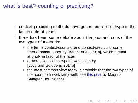
what is best? counting or predicting?

I context-predicting methods have generated a bit of hype in thelast couple of years

I there has been some debate about the pros and cons of thetwo types of methods:

I the terms �context-counting� and �context-predicting� comefrom a recent paper by [Baroni et al., 2014], which arguedstrongly in favor of the latter

I a more skeptical viewpoint was taken by[Levy and Goldberg, 2014b]

I the most common view today is probably that the two types ofmethods both work fairly well: see this post by MagnusSahlgren, for instance

-20pt

UNIVERSITY OF

GOTHENBURG

example: skip-gram with negative sampling (word2vec)

I the skip-gram with negative sampling (SGNS) model[Mikolov et al., 2013a]:

I we have one set of vectors for the target words, and anotherfor the contexts

I e.g. one target word vector for �pizza�, and a context vectorfor �is the object of eat�

I for each word�context pair, generate some random negativeexamples of contexts

I e.g. �pizza� + �is the object of persuade�

I SGNS trains a classi�er similar to logistic regression so thatI VT (pizza) · VC (object of eat) is highI VT (pizza) · VC (object of persuade) is low

-20pt

UNIVERSITY OF

GOTHENBURG

SGNS: pseudocode

for each word token W in the corpus�nd the context C of that occurrencefor each part c in the context C

update the context vector Vc for wupdate the word vector Vw for cfor each random negative example context n

update the context vector Vn for wupdate the word vector Vw for n

-20pt

UNIVERSITY OF

GOTHENBURG

some software (a small sample)

I word2vec: the software by Mikolov when he was atGoogle

I implements the SGNS model (and a few others)I includes a word space built by Google using a huge

collection of news text

I gensim: a nice Python library by �eh̊u°ekI includes a reimplementation of SGNS but also several

other useful algorithms, such as LSA and LDA

-20pt

UNIVERSITY OF

GOTHENBURG

word analogies and relational similarity

I relational similarity: how similar is the relation betweencat:tail to that between car:tyre?

I word analogy (Google test set): Moscow is to Russia asCopenhagen is to X?

I in some vector space models, we can get a reasonably goodanswer by a simple vector operation:

V (X ) = V (Copenhagen) + (V (Russia)− V (Moscow))

I then �nd the word whose vector is closest to V (X )I see [Mikolov et al., 2013b] and [Levy and Goldberg, 2014b]

-20pt

UNIVERSITY OF

GOTHENBURG

gender in the word space (example by Mikolov)

-20pt

UNIVERSITY OF

GOTHENBURG

example: countries and cities

0.6 0.4 0.2 0.0 0.2 0.4 0.60.8

0.6

0.4

0.2

0.0

0.2

0.4

0.6

Berlin

Tyskland

Stockholm

Sverige

Paris

Frankrike

Moskva

Ryssland

Köpenhamn

Danmark

Oslo

Norge

Tallinn

Estland

Rom

Italien

-20pt

UNIVERSITY OF

GOTHENBURG

distributional models as �simple semi-supervised� learning

I distributional models often give an improvement when addedas features to standard machine learning-based NLP systems

I this can be seen as a simple approach to semi-supervisedlearning:

I we have a small hand-labeled corpus (for instance, for traininga parser or named entity recognizer)

I we have a large unlabeled corpus: how can we do somethinguseful with it?

I the classical paper is by [Turian et al., 2010]; several morerecent ones [Guo et al., 2014]

-20pt

UNIVERSITY OF

GOTHENBURG

intuition (for instance, named entity recognition)

I instead of

Gothenburg → [0, 0, . . . , 0, 1, 0, . . .]Hargeisa → [0, 0, . . . , 0, 0, 1, . . .]

I . . . we can have

Gothenburg → [0.010,−0.20, . . . , 0.15, 0.07,−0.23, . . .]Hargeisa → [0.015,−0.05, . . . , 0.11, 0.14,−0.12, . . .]

-20pt

UNIVERSITY OF

GOTHENBURG

adding the distributional information

I straigtforward approach [Turian et al., 2010]:

I [Guo et al., 2014] and [Bansal et al., 2014] report that it'sbetter if we cluster the vectors before adding them as features

I example: word2vec vectors computed from a Spanish corpusclustered by k-means into 1000 clusters

282: juan, lázaro, joaquín, jaime, hugo, gastón, ...

441: mosca, mono, perro, pájaro, mamut, mandril, ...

844: estocolmo, gotenburgo, gotemburgo, dinamarca, ...

I mostly trial and error: what is best depends on the problemand on the learning algorithm used

-20pt

UNIVERSITY OF

GOTHENBURG

next lecture: predicting sequences and trees

United Nations o�cial Ekeus heads for Baghdad .

B-ORG I-ORG O B-PER O O B-LOC O

A C A T G G T C T G A A

N N C C C C C C C C C N

-20pt

UNIVERSITY OF

GOTHENBURG

references I

I Bansal, M., Gimpel, K., and Livescu, K. (2014). Tailoring continuous wordrepresentations for dependency parsing. In ACL.

I Baroni, M., Dinu, G., and Kruszewski, G. (2014). Don't count, predict! Asystematic comparison of context-counting vs. context-predicting semanticvectors. In ACL.

I Firth, J. (1957). Papers in Linguistics 1934�1951. OUP.

I Guo, J., Che, W., Wang, H., and Liu, T. (2014). Revisiting embeddingfeatures for simple semi-supervised learning. In EMNLP.

I Kanerva, P., Kristo�ersson, J., and Holst, A. (2000). Random indexing oftext samples for latent semantic analysis. In Proceedings of the 22nd Annual

Conference of the Cognitive Science Society.

I Landauer, T. K. and Dumais, S. T. (1997). A solution to Plato's problem:The latent semantic analysis theory of acquisition, induction andrepresentation of knowledge. Psychological Review, 104:211�240.

I Lazaridou, A., Pham, N. T., and Baroni, M. (2015). Combining languageand vision with a multimodal skipgram model. In NAACL.

-20pt

UNIVERSITY OF

GOTHENBURG

references II

I Lenci, A. (2008). Distributional semantics in linguistic and cognitiveresearch. Rivista di Linguistica, 20(1).

I Levy, O. and Goldberg, Y. (2014a). Dependency-based word embeddings. InACL.

I Levy, O. and Goldberg, Y. (2014b). Linguistic regularities in sparse andexplicit word representations. In Proceedings of CoNLL.

I Mikolov, T., Sutskever, I., Chen, K., Corrado, G., and Dean, J. (2013a).Distributed representations of words and phrases and their compositionality.In NIPS.

I Mikolov, T., Yih, W.-t., and Zweig, G. (2013b). Linguistic regularities incontinuous space word representations. In Proc. NAACL.

I Padó, S. and Lapata, M. (2007). Dependency-based construction ofsemantic space models. Computational Linguistics, 33(1).

I Sahlgren, M. (2006). The Word-Space Model. PhD thesis, StockholmUniversity.

-20pt

UNIVERSITY OF

GOTHENBURG

references III

I Turian, J., Ratinov, L.-A., and Bengio, Y. (2010). Word representations: Asimple and general method for semi-supervised learning. In Proc. ACL.