Machine Learningfor natural language processingPCFG: Parameter estimation with EM

Laura Kallmeyer

Heinrich-Heine-Universitat Dusseldorf

Summer 2016

1 / 30

Introduction

Unsupervised parameter estimation for HMMs has been donewith the EM algorithm, based on the forward and backwardprobabilities.EM can be used more generally for unsupervised parameterestimation with generative models (Dempster et al., 1977).Today: introduction of PCFG, inside and outside probabilitiesand unsupervised estimation of the probabilities of the PCFGusing EM based on inside and outside probabilities.

Booth (1969); Pereira & Schabes (1992); Collins; Petrov et al. (2006)

2 / 30

Table of contents

1 Motivation

2 PCFG

3 Inside and outside computation

4 EM Training for probability estimation

5 Treebank re�nement

3 / 30

Motivation

Probabilistic Context-Free Grammars (PCFG)

are CFGs with probabilities a�ached to productionsare widely used for data-driven constituency parsing

�e probabilities can be estimated from unannotated data via the EMalgorithm, based on inside and outside probabilities, similar toestimating HMM parameter with forward and backward probabilities.

4 / 30

Motivation

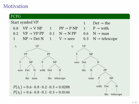
PCFGStart symbol VP0.8 VP→ V NP0.2 VP→ VP PP1 NP→ Det N

1 PP→ P NP0.1 N→ N PP1 V→ sees

1 Det→ the1 P→ with0.6 N→ man0.3 N→ telescope

t1 VP

PP

NP

N

telescope

Det

the

P

with

VP

NP

N

man

Det

the

V

sees

t2 VP

NP

N

PP

NP

N

telescope

Det

the

P

with

N

man

Det

the

V

sees

P(t1) = 0.6 ⋅ 0.8 ⋅ 0.2 ⋅ 0.3 = 0.0288P(t2) = 0.6 ⋅ 0.8 ⋅ 0.1 ⋅ 0.3 = 0.0144

5 / 30

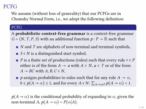
PCFGWe assume (without loss of generality) that our PCFGs are inChomsky Normal Form, i.e., we adopt the following de�nition:

PCFGA probabilistic context-free grammar is a context-free grammarG = ⟨N ,T ,P, S⟩ with an additional function p ∶ P → R such that

N and T are alphabets of non-terminal and terminal symbols,S ∈ N is a distinguished start symbol,P is a �nite set of productions (rules) such that every rule r ∈ Peither is of the form A → a with A ∈ N ,a ∈ T or of the formA→ BC with A,B,C ∈ N ,p assigns probabilities to rules such that for any rule A → α,0 ≤ p(A→ α) ≤ 1, and for every A ∈ N : ∑A→α∈P p(A→ α) = 1.

p(A→ α) is the conditional probability of expanding to α, given thenon-terminal A, p(A→ α) = P(α∣A).

6 / 30

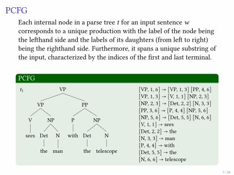
PCFGEach internal node in a parse tree t for an input sentence wcorresponds to a unique production with the label of the node beingthe le�hand side and the labels of its daughters (from le� to right)being the righthand side. Furthermore, it spans a unique substring ofthe input, characterized by the indices of the �rst and last terminal.

PCFGt1 VP

PP

NP

N

telescope

Det

the

P

with

VP

NP

N

man

Det

the

V

sees

[VP, 1, 6] → [VP, 1, 3] [PP, 4, 6][VP, 1, 3] → [V, 1, 1] [NP, 2, 3][NP, 2, 3] → [Det, 2, 2] [N, 3, 3][PP, 3, 6] → [P, 4, 4] [NP, 5, 6][NP, 5, 6] → [Det, 5, 5] [N, 6, 6][V, 1, 1] → sees[Det, 2, 2] → the[N, 3, 3] → man[P, 4, 4] → with[Det, 5, 5] → the[N, 6, 6] → telescope

7 / 30

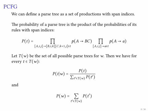
PCFGWe can de�ne a parse tree as a set of productions with span indices.

�e probability of a parse tree is the product of the probabilities of itsrules with span indices:

P(t) = ∏[A,i,j]→[B,i,k][C,k+1,j]∈t

p(A→ BC) ∏[A,i,j]→a∈t

p(A→ a)

Let T(w) be the set of all possible parse trees for w. �en we have forevery t ∈ T(w):

P(t∣w) = P(t)∑t′∈T(w) P(t′)

and

P(w) = ∑t′∈T(w)

P(t′)

8 / 30

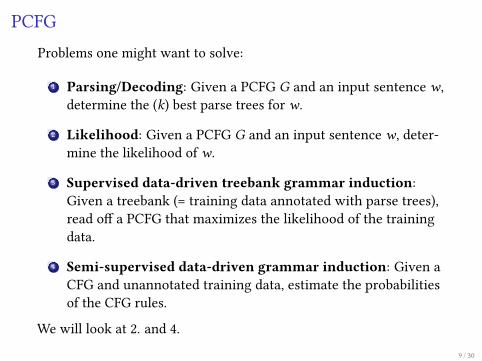
PCFGProblems one might want to solve:

1 Parsing/Decoding: Given a PCFG G and an input sentence w,determine the (k) best parse trees for w.

2 Likelihood: Given a PCFG G and an input sentence w, deter-mine the likelihood of w.

3 Supervised data-driven treebank grammar induction:Given a treebank (= training data annotated with parse trees),read o� a PCFG that maximizes the likelihood of the trainingdata.

4 Semi-supervised data-driven grammar induction: Given aCFG and unannotated training data, estimate the probabilitiesof the CFG rules.

We will look at 2. and 4.

9 / 30

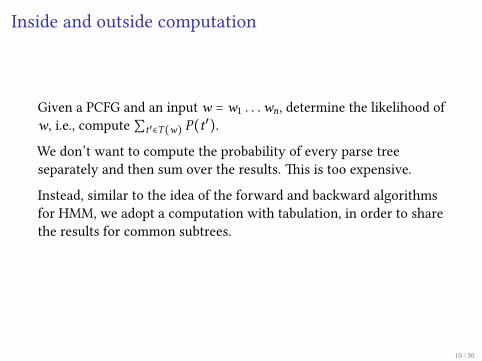
Inside and outside computation

Given a PCFG and an input w = w1 . . .wn, determine the likelihood ofw, i.e., compute ∑t′∈T(w) P(t′).We don’t want to compute the probability of every parse treeseparately and then sum over the results. �is is too expensive.

Instead, similar to the idea of the forward and backward algorithmsfor HMM, we adopt a computation with tabulation, in order to sharethe results for common subtrees.

10 / 30

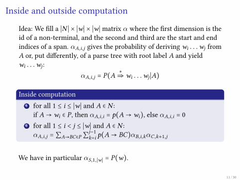
Inside and outside computation

Idea: We �ll a ∣N ∣ × ∣w∣ × ∣w∣ matrix α where the �rst dimension is theid of a non-terminal, and the second and third are the start and endindices of a span. αA,i,j gives the probability of deriving wi . . .wj fromA or, put di�erently, of a parse tree with root label A and yieldwi . . .wj :

αA,i,j = P(A ∗⇒ wi . . .wj ∣A)

Inside computation1 for all 1 ≤ i ≤ ∣w∣ and A ∈ N :

if A→ wi ∈ P , then αA,i,i = p(A→ wi), else αA,i,i = 02 for all 1 ≤ i < j ≤ ∣w∣ and A ∈ N :αA,i,j = ∑A→BC∈P ∑j−1

k=i p(A→ BC)αB,i,kαC,k+1,j

We have in particular αS,1,∣w∣ = P(w).

11 / 30

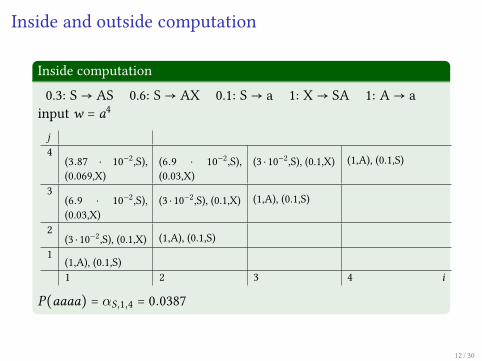
Inside and outside computation

Inside computation

0.3: S→ AS 0.6: S→ AX 0.1: S→ a 1: X→ SA 1: A→ ainput w = a4

j4

(3.87 ⋅ 10−2,S),(0.069,X)

(6.9 ⋅ 10−2,S),(0.03,X)

(3 ⋅ 10−2,S), (0.1,X) (1,A), (0.1,S)

3(6.9 ⋅ 10−2,S),(0.03,X)

(3 ⋅ 10−2,S), (0.1,X) (1,A), (0.1,S)

2(3 ⋅ 10−2,S), (0.1,X) (1,A), (0.1,S)

1(1,A), (0.1,S)1 2 3 4 i

P(aaaa) = αS,1,4 = 0.0387

12 / 30

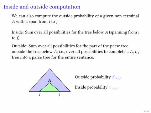
Inside and outside computationWe can also compute the outside probability of a given non-terminalA with a span from i to j.

Inside: Sum over all possibilities for the tree below A (spanning from ito j).

Outside: Sum over all possibilities for the part of the parse treeoutside the tree below A, i.e., over all possibilities to complete a A, i, jtree into a parse tree for the entire sentence.

A

i j

AOutside probability βA,i,j

Inside probability αA,i,j

13 / 30

Inside and outside computation

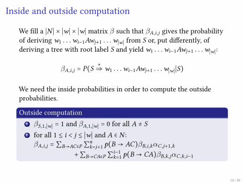
We �ll a ∣N ∣ × ∣w∣ × ∣w∣ matrix β such that βA,i,j gives the probabilityof deriving w1 . . .wi−1Awj+1 . . .w∣w∣ from S or, put di�erently, ofderiving a tree with root label S and yield w1 . . .wi−1Awj+1 . . .w∣w∣:

βA,i,j = P(S ∗⇒ w1 . . .wi−1Awj+1 . . .w∣w∣∣S)

We need the inside probabilities in order to compute the outsideprobabilities.

Outside computation1 βS,1,∣w∣ = 1 and βA,1,∣w∣ = 0 for all A ≠ S2 for all 1 ≤ i < j ≤ ∣w∣ and A ∈ N :βA,i,j = ∑B→AC∈P ∑n

k=j+1 p(B → AC)βB,i,kαC,j+1,k+∑B→CA∈P ∑i−1

k=1 p(B → CA)βB,k,jαC,k,i−1

14 / 30

Inside and outside computation

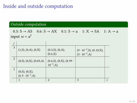
Outside computation

0.3: S→ AS 0.6: S→ AX 0.1: S→ a 1: X→ SA 1: A→ ainput w = a3

j3

(1,S), (0,A), (0,X) (0.3,S), (0,A),(0.6,X)

(9 ⋅ 10−2,S), (0.18,X),(3 ⋅ 10−2,A)

2(0,S), (0,X), (0.03,A) (0.6,S), (0,X), (8.99 ⋅

10−3,A)1

(0,S), (0,X),(6.9 ⋅ 10−2,A)1 2 3 i

15 / 30

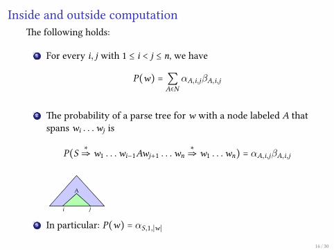
Inside and outside computation�e following holds:

1 For every i, j with 1 ≤ i < j ≤ n, we have

P(w) = ∑A∈N

αA,i,jβA,i,j

2 �e probability of a parse tree for w with a node labeled A thatspans wi . . .wj is

P(S ∗⇒ w1 . . .wi−1Awj+1 . . .wn∗⇒ w1 . . .wn) = αA,i,jβA,i,j

A

i j

A

3 In particular: P(w) = αS,1,∣w∣

16 / 30

Training

Supervised data-driven PCFG parsing: Given a treebank, read o� therules and estimate their probabilities based on the counts of the rules.

More challenging: Unsupervised parameter estimation: Given a CFGand unannotated training data, estimate the probabilities of the rules.

We use the EM algorithm, based on the inside and outsidecomputations from the previous slides.

17 / 30

Training

Underlying ideas, as in the HMM parameter estimation:

We estimate parameters iteratively: we start with some param-eters and use the estimated probabilities to derive be�er andbe�er parameters.

We use our current parameters to estimate (fractional) countsof possible parse trees and possible rules. In other words,the probability mass assigned to the training corpus gets dis-tributed among the possible parse trees.

�ese fractional counts are then used to compute the parame-ters of the next model.

18 / 30

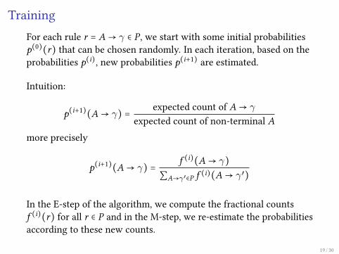
TrainingFor each rule r = A→ γ ∈ P , we start with some initial probabilitiesp(0)(r) that can be chosen randomly. In each iteration, based on theprobabilities p(i), new probabilities p(i+1) are estimated.

Intuition:

p(i+1)(A→ γ) = expected count of A→ γ

expected count of non-terminal Amore precisely

p(i+1)(A→ γ) = f (i)(A→ γ)∑A→γ′∈P f (i)(A→ γ′)

In the E-step of the algorithm, we compute the fractional countsf (i)(r) for all r ∈ P and in the M-step, we re-estimate the probabilitiesaccording to these new counts.

19 / 30

TrainingWe can think of this as follows:

Our training data are sentences w(1), . . . ,w(N).

In each iteration, based on the current probabilities, we create atreebank for training:

For each of the sentences, the treebank contains all possibleparse trees. But tree t does not occur once in the treebank,instead, it occurs P(t) times.

Consequently, when counting occurrences of rules in the tree-bank in order to estimate new probabilities, an occurrence ofsome rule r in a parse tree t does not add 1 to the count but itadds P(t).

�e resulting count for rule r , summing up the probabilities ofthe parse trees for every occurrence of r , is then the exptectedcount of r .

20 / 30

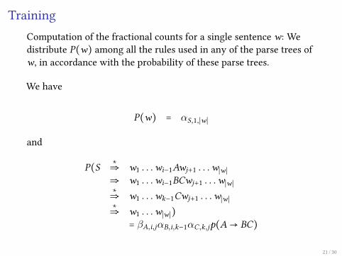
TrainingComputation of the fractional counts for a single sentence w: Wedistribute P(w) among all the rules used in any of the parse trees ofw, in accordance with the probability of these parse trees.

We have

P(w) = αS,1,∣w∣

and

P(S ∗⇒ w1 . . .wi−1Awj+1 . . .w∣w∣⇒ w1 . . .wi−1BCwj+1 . . .w∣w∣∗⇒ w1 . . .wk−1Cwj+1 . . .w∣w∣∗⇒ w1 . . .w∣w∣)

= βA,i,jαB,i,k−1αC,k,jp(A→ BC)

21 / 30

Training

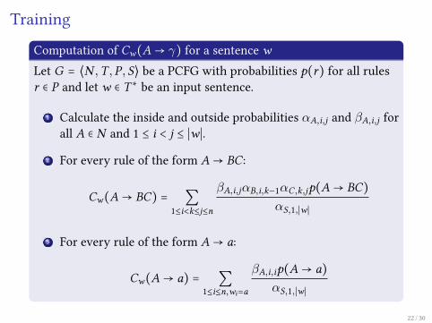
Computation of Cw(A→ γ) for a sentence wLet G = ⟨N ,T ,P, S⟩ be a PCFG with probabilities p(r) for all rulesr ∈ P and let w ∈ T∗ be an input sentence.

1 Calculate the inside and outside probabilities αA,i,j and βA,i,j forall A ∈ N and 1 ≤ i < j ≤ ∣w∣.

2 For every rule of the form A→ BC:

Cw(A→ BC) = ∑1≤i<k≤j≤n

βA,i,jαB,i,k−1αC,k,jp(A→ BC)αS,1,∣w∣

3 For every rule of the form A→ a:

Cw(A→ a) = ∑1≤i≤n,wi=a

βA,i,ip(A→ a)αS,1,∣w∣

22 / 30

Training

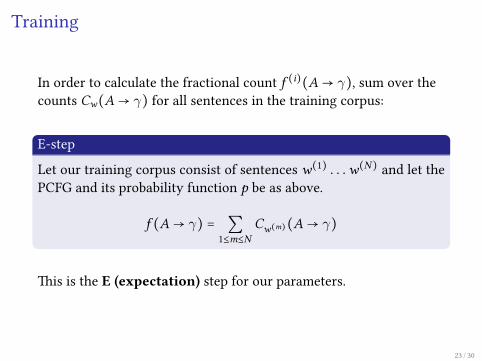
In order to calculate the fractional count f (i)(A→ γ), sum over thecounts Cw(A→ γ) for all sentences in the training corpus:

E-step

Let our training corpus consist of sentences w(1) . . .w(N) and let thePCFG and its probability function p be as above.

f (A→ γ) = ∑1≤m≤N

Cw(m)(A→ γ)

�is is the E (expectation) step for our parameters.

23 / 30

Training

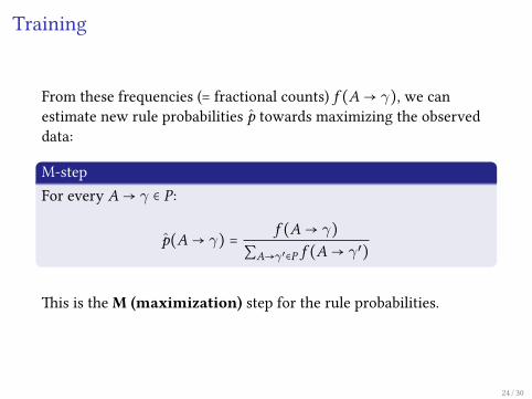
From these frequencies (= fractional counts) f (A→ γ), we canestimate new rule probabilities p towards maximizing the observeddata:

M-stepFor every A→ γ ∈ P :

p(A→ γ) = f (A→ γ)∑A→γ′∈P f (A→ γ′)

�is is theM (maximization) step for the rule probabilities.

24 / 30

Training

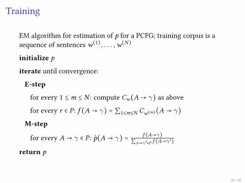
EM algorithm for estimation of p for a PCFG; training corpus is asequence of sentences w(1), . . . ,w(N)

initialize p

iterate until convergence:

E-step

for every 1 ≤ m ≤ N : compute Cw(A→ γ) as abovefor every r ∈ P : f (A→ γ) = ∑1≤m≤N Cw(m)(A→ γ)

M-step

for every A→ γ ∈ P : p(A→ γ) = f (A→γ)∑A→γ′∈P f (A→γ′)

return p

25 / 30

Treebank re�nement

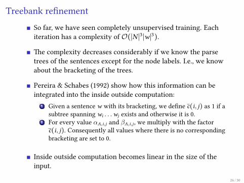
So far, we have seen completely unsupervised training. Eachiteration has a complexity of O(∣N ∣3∣w∣3).

�e complexity decreases considerably if we know the parsetrees of the sentences except for the node labels. I.e., we knowabout the bracketing of the trees.

Pereira & Schabes (1992) show how this information can beintegrated into the inside outside computation:

1 Given a sentence w with its bracketing, we de�ne c(i, j) as 1 if asubtree spanning wi . . .wj exists and otherwise it is 0.

2 For every value αA,i,j and βA,i,j , we multiply with the factorc(i, j). Consequently all values where there is no correspondingbracketing are set to 0.

Inside outside computation becomes linear in the size of theinput.

26 / 30

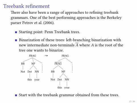
Treebank re�nement�ere also have been a range of approaches to re�ning treebankgrammars. One of the best performing approaches is the Berkeleyparser Petrov et al. (2006).

Starting point: Penn Treebank trees.

Binarization of these trees: le�-branching binarization withnew intermediate non-terminals A where A is the root of thetree one wants to binarize.

FRAG

.

.

NP

NN

year

Det

this

RB

Not

↝ FRAG

.

.

FRAG

NP

NN

year

Det

this

RB

Not

Start with the treebank grammar obtained from these trees.27 / 30

Treebank re�nementIteration for learning new labels and estimating new probabilities:

Given a current PCFG, repeat the following until no more successfulsplits can be found:

Split non-terminals:

Split every non-terminal A into 2 new symbols A1,A2(e.g, NP↝NP1, NP2),

replace every rule A → α with A1 → α and A2 → α, both withthe same probability as the original rule,

and for every occurrence of A in a righthand side of some B →γ, replace B → γ with two new rules, one with A1 instead of Aand another one with A2, dividing the probability of the originalrule between these two new rules. �is is done repeatedly untilall old non-terminals have been removed.

Furthermore, add some small amount of randomness to theprobabilities to break the symmetry.

28 / 30

Treebank re�nement

�en, probabilities are re-estimating using the inside-outsideEM algorithm with the spli�ed grammar, based on the correcttreebank bracketing and the coarser node labels in the tree-bank.

Each split that has contributed to increasing the probability ofthe training data is kept and the other splits are reversed.

Result:

POS tags get split, for instance VBZ is split into 11 di�erentPOS tags.Phrasal non-terminals get split as well, for example di�erentVP categories for in�nite VPs, passive VPs, intransitive VPs etc.�e best evaluation was obtained with a resulting grammarwith 1043 symbols, F1 score of 90.2% on the Penn treebank.

29 / 30

References

Booth, T. 1969. Probabilistic representation of formal languages. In Tenth annual ieeesymposium on switching and automata theory, .

Collins, Michael. �� �e inside-outside algorithm.www.cs.columbia.edu/∼mcollins/io.pdf.

Dempster, A. P., N. M. Laird & D. B. Rubin. 1977. Maximum likelihood fromincomplete data via the EM algorithm. Journal of the Royal Statistical Society 39(1).1–21.

Pereira, Fernando & Yves Schabes. 1992. Inside-outside reestimation from partiallybracketed corpora. In Proceedings of the 30th annual meeting of the association forcomputational linguistics, 128–135. Newark, Delaware, USA: Association forComputational Linguistics. doi:10.3115/981967.981984.http://www.aclweb.org/anthology/P92-1017.

Petrov, Slav, Leon Barre�, Romain �ibaux & Dan Klein. 2006. Learning Accurate,Compact, and Interpretable Tree Annotation. In Proceedings of the 21stinternational conference on computational linguistics and 44th annual meeting of theacl, 433–440. Sydney.

30 / 30