Machine Learning for Astronomy

Rob Fergus

Dept. of Computer Science,Courant Institute,

New York University

• High-level view of machine learning– Discuss generative & discriminative modeling of data– Not exhaustive survey– Try to illustrate important ML concepts

• Give examples of these models applied to problems in astronomy

• In particular, exoplanet detection algorithms

Overview

Generative vs Discriminative Modeling

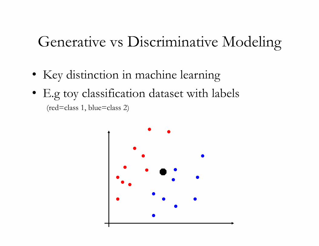
• Key distinction in machine learning• E.g toy classification dataset with labels

(red=class 1, blue=class 2)

Generative vs Discriminative Modeling

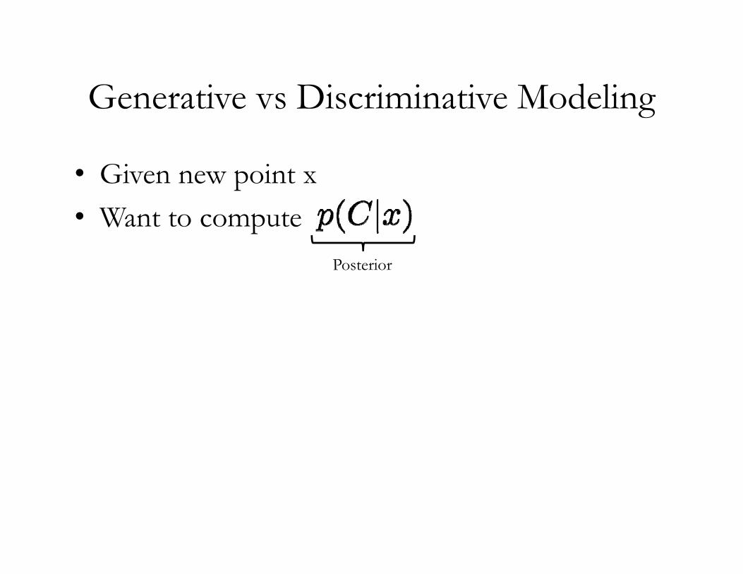
• Given new point x• Want to compute

• Alternatively:Posterior Likelihood Prior

Discriminativeapproaches

compute this

Generativeapproaches

compute this

Bayes rule

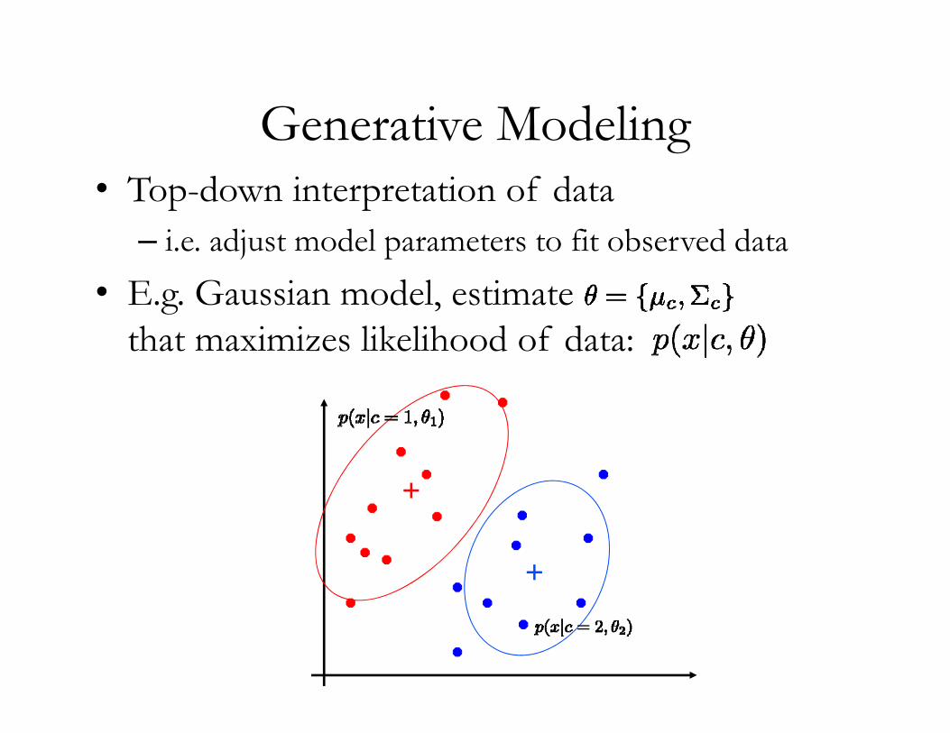
Generative Modeling• Top-down interpretation of data

– i.e. adjust model parameters to fit observed data• E.g. Gaussian model, estimate

that maximizes likelihood of data:

+

+

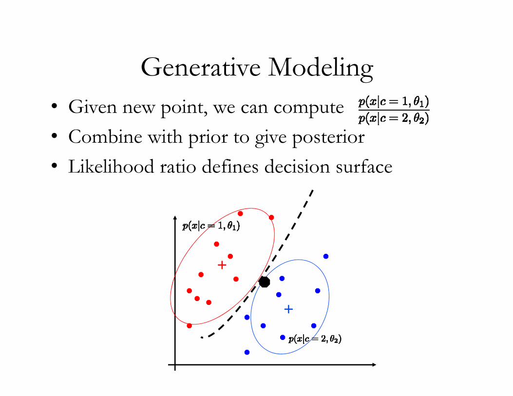
Generative Modeling• Given new point, we can compute • Combine with prior to give posterior• Likelihood ratio defines decision surface

+

+

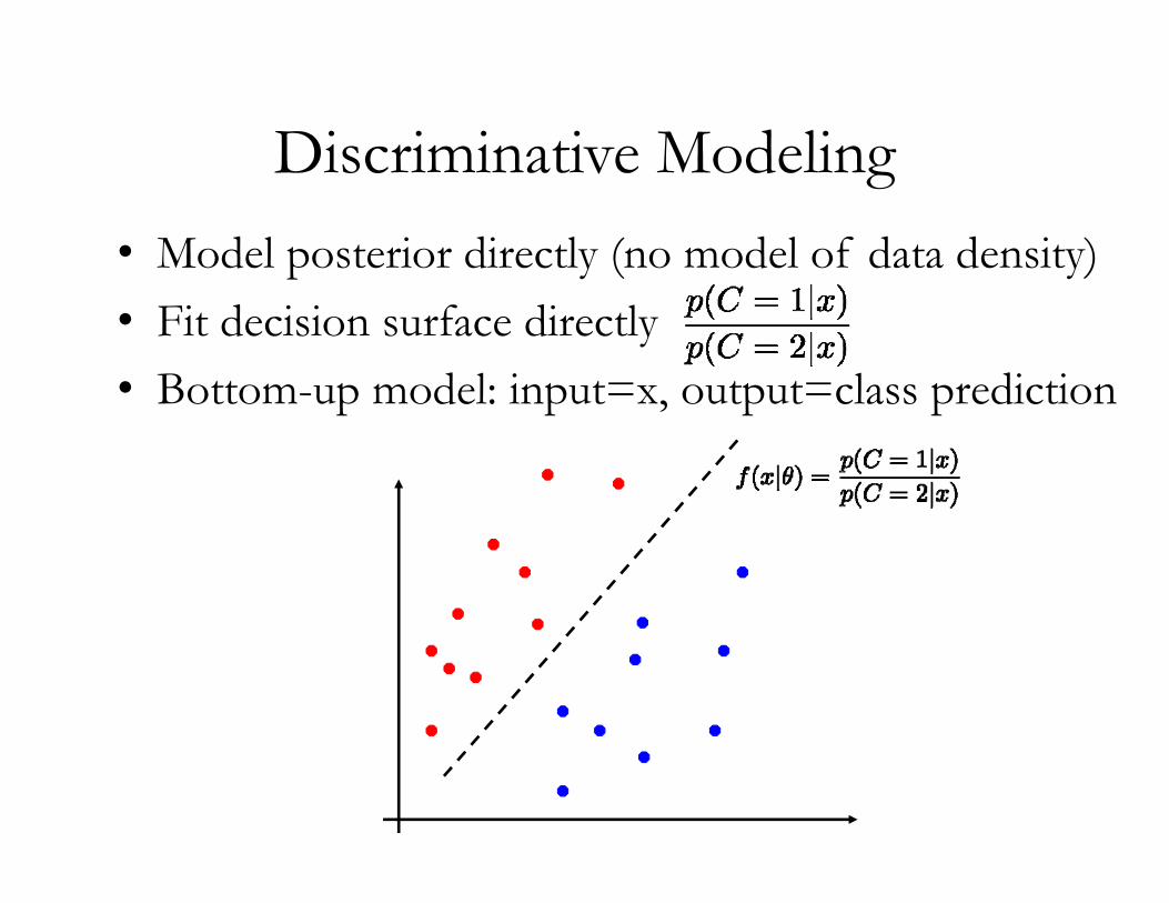
Discriminative Modeling• Model posterior directly (no model of data density)• Fit decision surface directly• Bottom-up model: input=x, output=class prediction

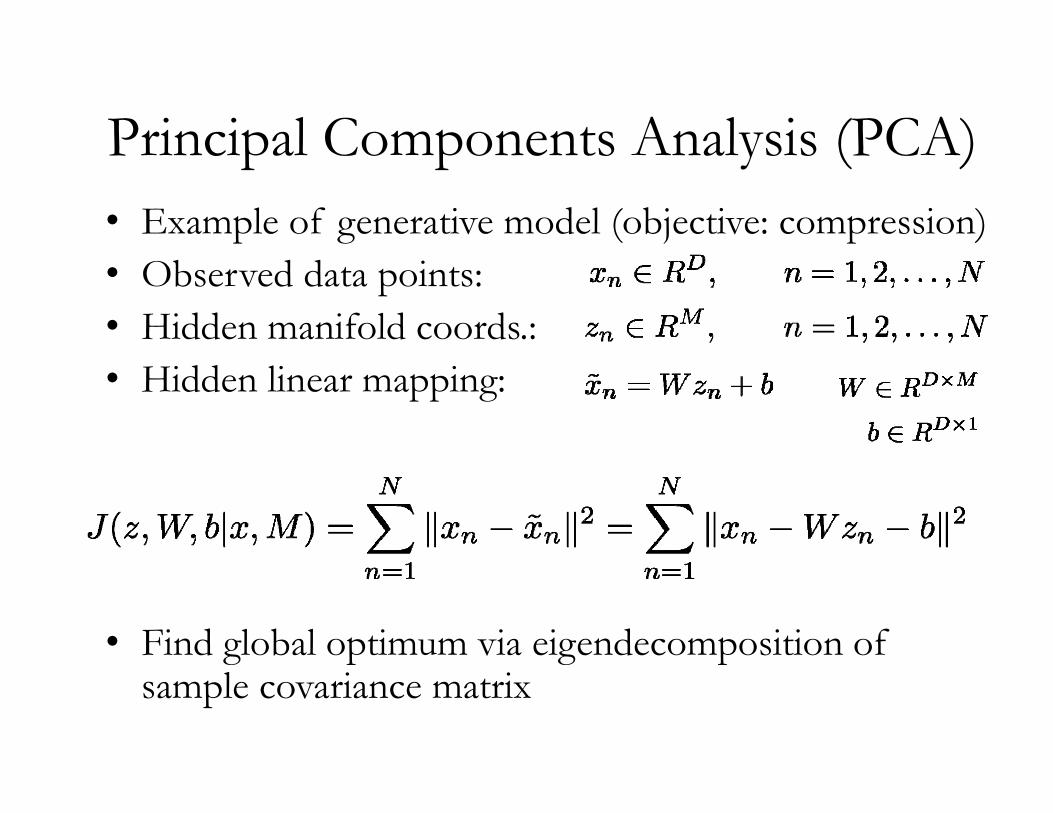
Principal Components Analysis (PCA)• Example of generative model (objective: compression)• Observed data points: • Hidden manifold coords.:• Hidden linear mapping:

• Find global optimum via eigendecomposition of sample covariance matrix

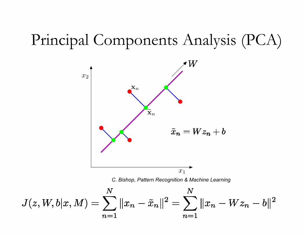
Principal Components Analysis (PCA)

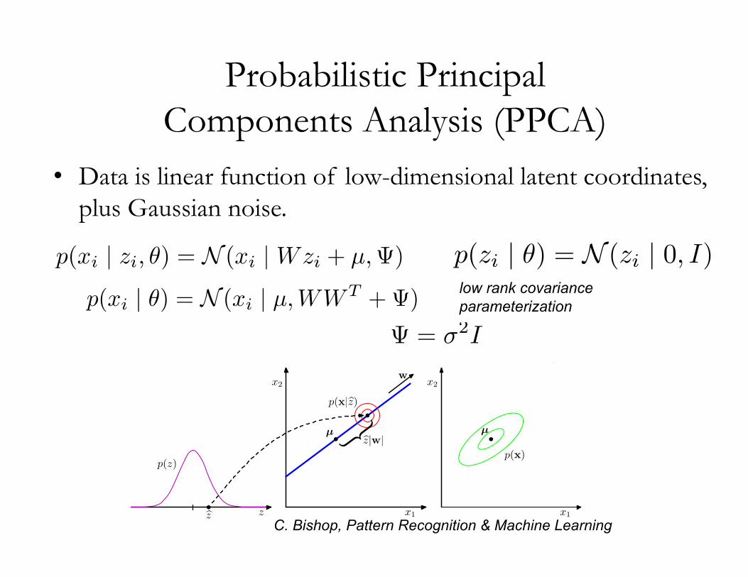
Probabilistic Principal Components Analysis (PPCA)

• Data is linear function of low-dimensional latent coordinates, plus Gaussian noise.

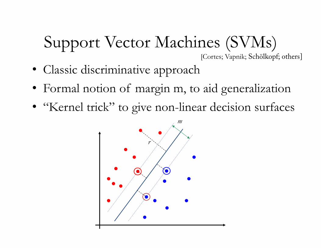
Support Vector Machines (SVMs)• Classic discriminative approach• Formal notion of margin m, to aid generalization• “Kernel trick” to give non-linear decision surfaces

r

m

[Cortes; Vapnik; Schölkopf; others]

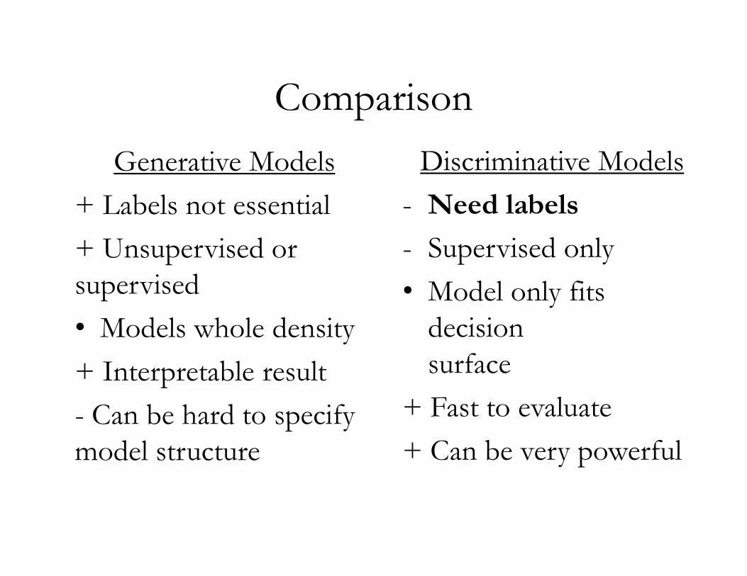
ComparisonGenerative Models

+ Labels not essential+ Unsupervised or supervised• Models whole density+ Interpretable result- Can be hard to specify model structure

Discriminative Models- Need labels

- Supervised only• Model only fits

decision surface

+ Fast to evaluate+ Can be very powerful

Detour

Deep Neural Networks for Natural Image Classification

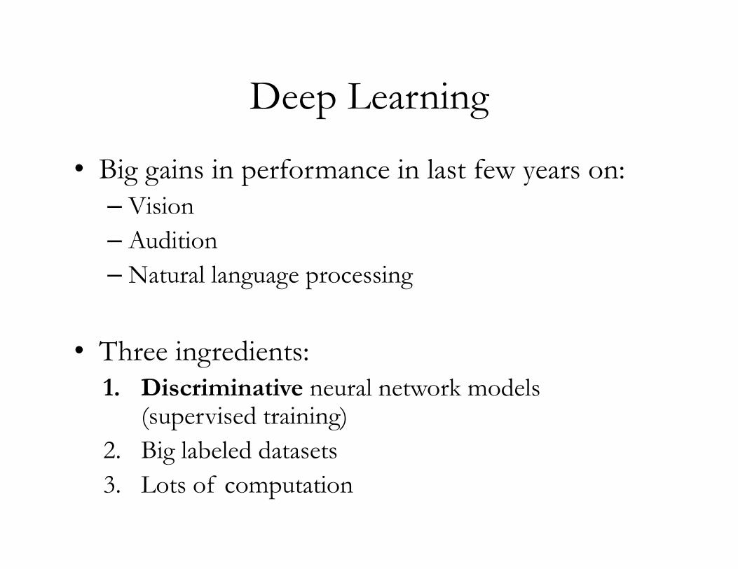
Deep Learning

• Big gains in performance in last few years on:– Vision– Audition– Natural language processing

• Three ingredients:1. Discriminative neural network models

(supervised training)2. Big labeled datasets3. Lots of computation

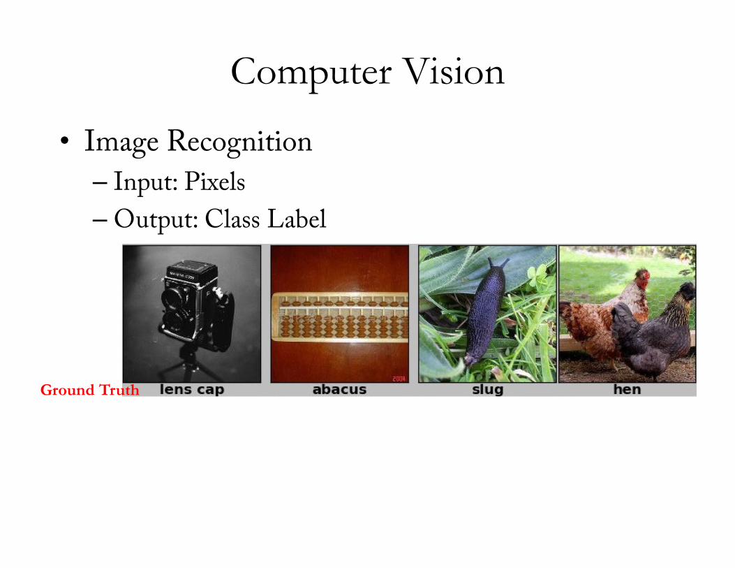
Computer Vision

[Krizhevsky et al. NIPS 2012]

• Image Recognition

– Input: Pixels

– Output: Class Label

Ground Truth

Model Predictions

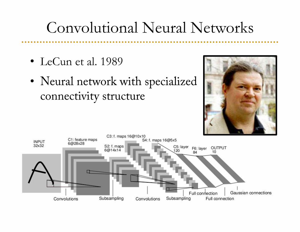
Convolutional Neural Networks

• LeCun et al. 1989

• Neural network with specialized connectivity structure

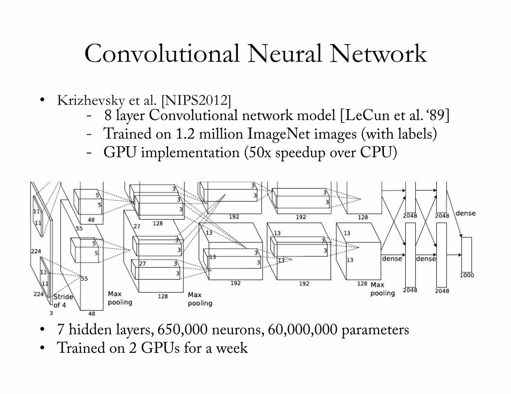
Convolutional Neural Network

• 7 hidden layers, 650,000 neurons, 60,000,000 parameters• Trained on 2 GPUs for a week

• Krizhevsky et al. [NIPS2012] - 8 layer Convolutional network model [LeCun et al. ‘89]- Trained on 1.2 million ImageNet images (with labels)- GPU implementation (50x speedup over CPU)

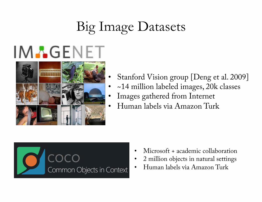
Big Image Datasets

[Deng et al. CVPR 2009]

• Stanford Vision group [Deng et al. 2009]• ~14 million labeled images, 20k classes• Images gathered from Internet

• Human labels via Amazon Turk

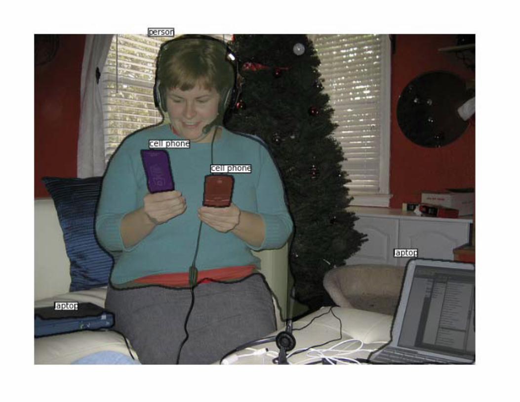
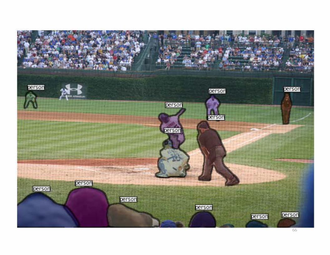
• Microsoft + academic collaboration• 2 million objects in natural settings

• Human labels via Amazon Turk

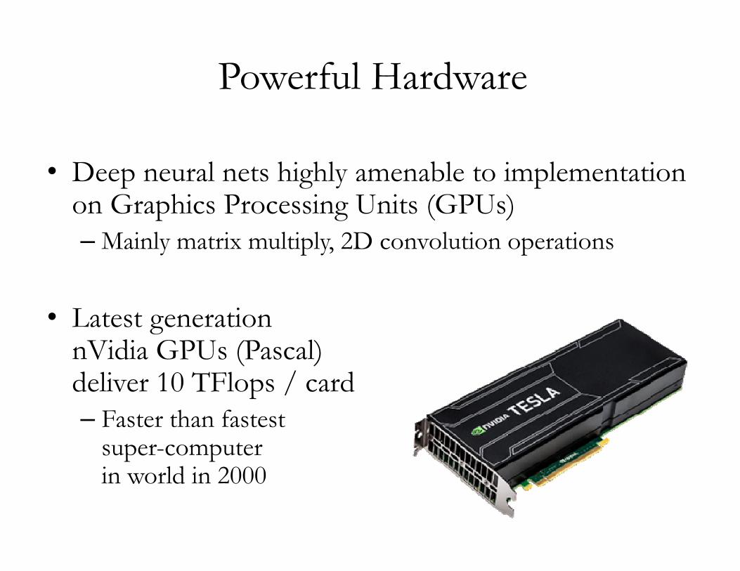
Powerful Hardware

• Deep neural nets highly amenable to implementation on Graphics Processing Units (GPUs)– Mainly matrix multiply, 2D convolution operations

• Latest generationnVidia GPUs (Pascal)deliver 10 TFlops / card– Faster than fastest

super-computerin world in 2000

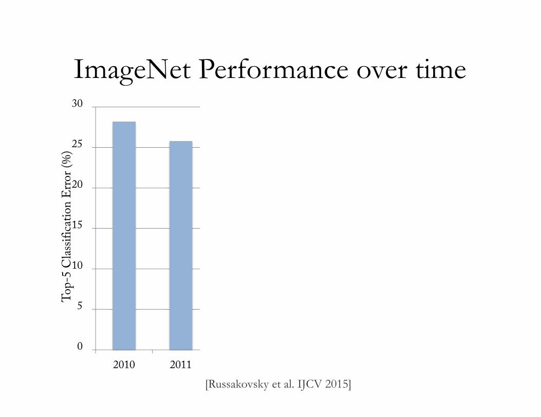
ImageNet Performance over time

0

5

10

15

20

25

30

2010 2011 2012 2013 2014 Human

Top

-5 C

lass

ific

atio

n E

rror

(%

)

2015

Convolutional

Neural Nets

[Russakovsky et al. IJCV 2015]

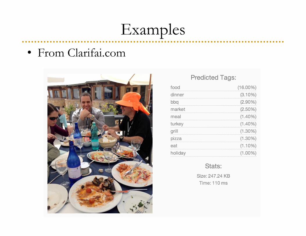
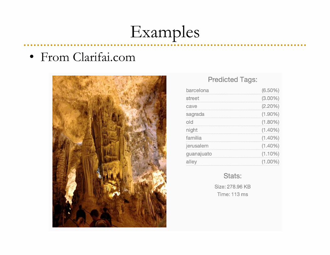
Examples• From Clarifai.com

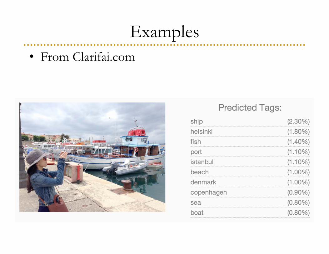
Examples• From Clarifai.com

Examples• From Clarifai.com

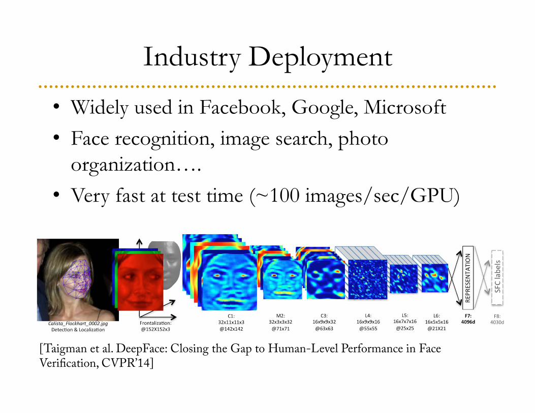
Industry Deployment

• Widely used in Facebook, Google, Microsoft• Face recognition, image search, photo

organization….• Very fast at test time (~100 images/sec/GPU)

[Taigman et al. DeepFace: Closing the Gap to Human-Level Performance in Face Verification, CVPR’14]

Success of DeepNets

• ConvNets work great for other types of data:– Medical imaging– Speech spectrograms– Particle physics traces

• Other types of deep neural nets (Recurrent Nets) work well for natural language

• But need lots and lots of labeled data!!

End of Detour

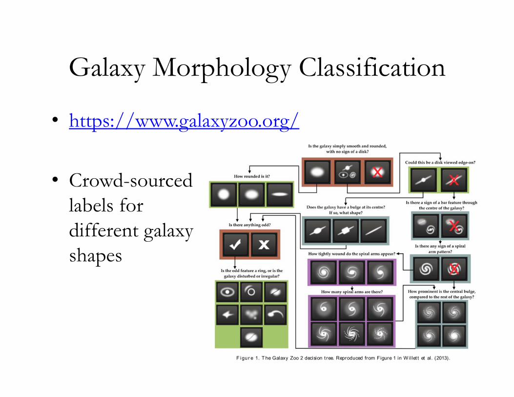
Galaxy Morphology Classification

• https://www.galaxyzoo.org/

• Crowd-sourcedlabels for different galaxyshapes

F igur e 1. T he Galaxy Zoo 2 decision t ree. Reproduced from Figure 1 in W illet t et al. (2013).

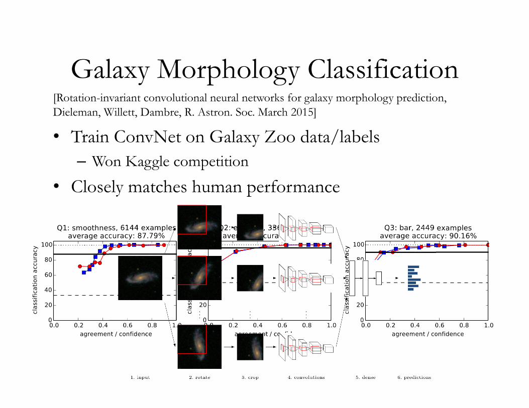
Galaxy Morphology Classification

• Train ConvNet on Galaxy Zoo data/labels– Won Kaggle competition

• Closely matches human performance

[Rotation-invariant convolutional neural networks for galaxy morphology prediction, Dieleman, Willett, Dambre, R. Astron. Soc. March 2015]

Direct Detection of Exoplanetsusing the S4 Algorithm[Spatio-Spectral Speckle Suppression]

Rob Fergus 1, David W. Hogg 2, Rebecca Oppenheimer 3, Doug Brenner 3, Laurent Pueyo 4

3 Dept. of AstrophysicsAmerican Museumof Natural History

2 Center for Cosmology & Particle Physics, Dept. of Physics,

New York University

1 Dept. of Computer Science,Courant Institute, New York University

4 Space TelescopeScience Institute

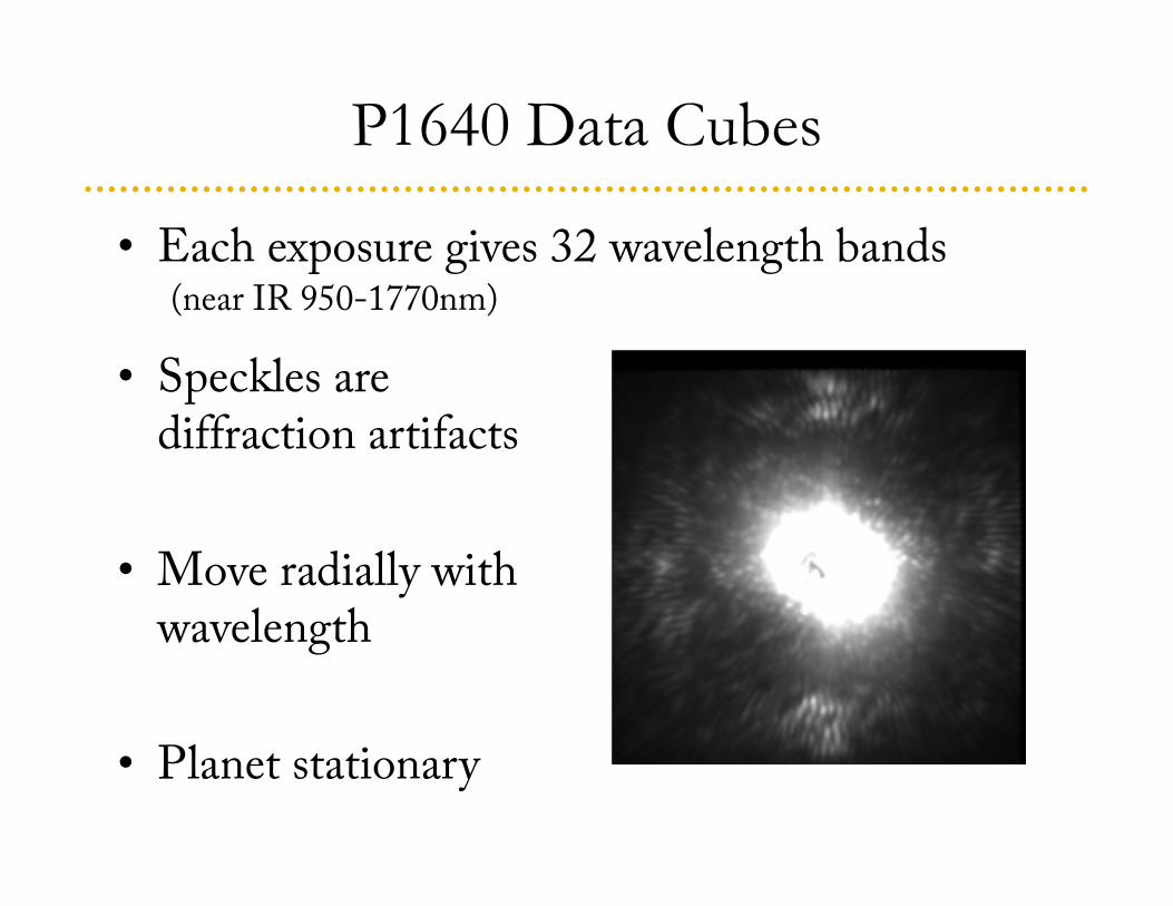
P1640 Data Cubes

• Each exposure gives 32 wavelength bands(near IR 950-1770nm)

• Speckles are diffraction artifacts

• Move radially with wavelength

• Planet stationary

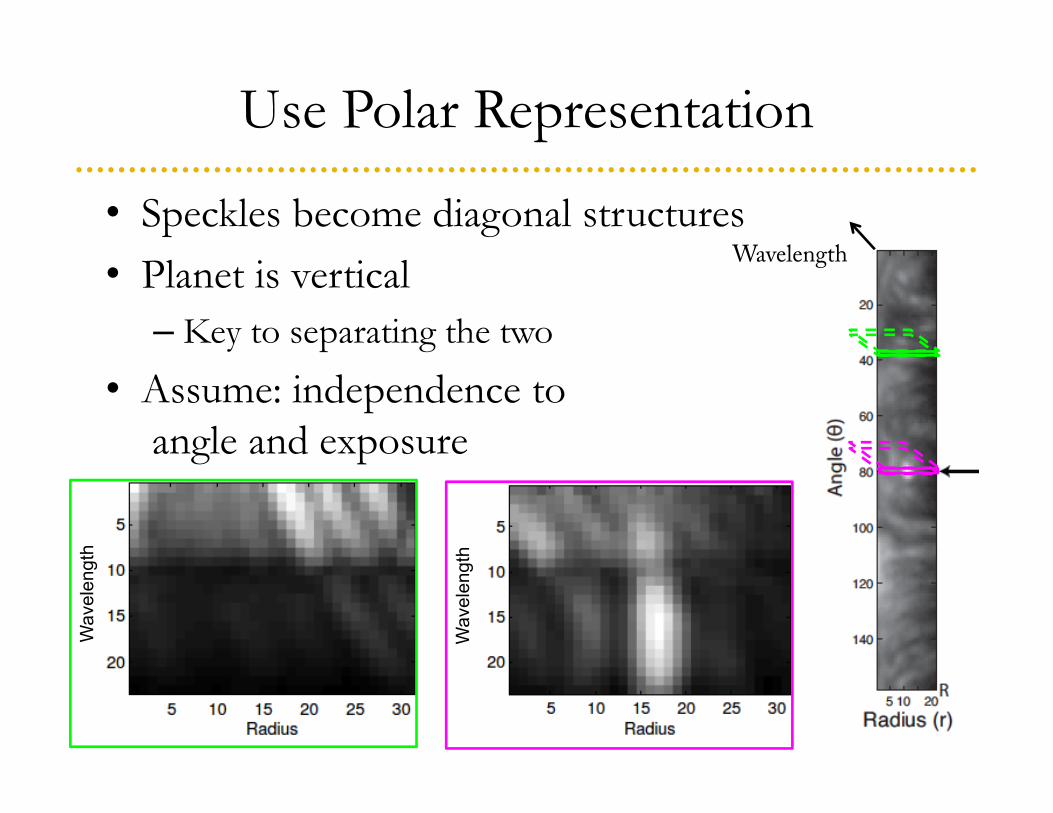
Use Polar Representation

• Speckles become diagonal structures• Planet is vertical

– Key to separating the two• Assume: independence to

angle and exposure W

avel

engt

h

Wav

elen

gth

Wavelength

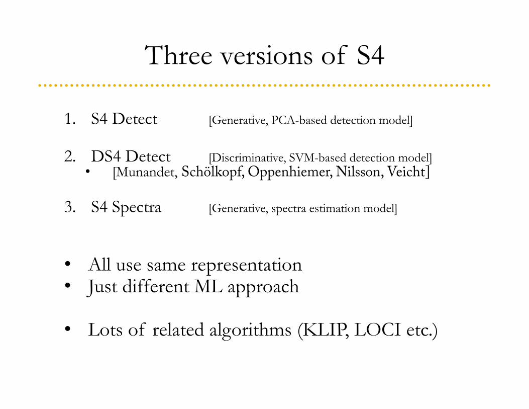
Three versions of S4

1. S4 Detect [Generative, PCA-based detection model]

2. DS4 Detect [Discriminative, SVM-based detection model]• [Munandet, Schölkopf, Oppenhiemer, Nilsson, Veicht]

3. S4 Spectra [Generative, spectra estimation model]

• All use same representation• Just different ML approach

• Lots of related algorithms (KLIP, LOCI etc.)

[Fergus et al., Astrophysical Journal, under review]

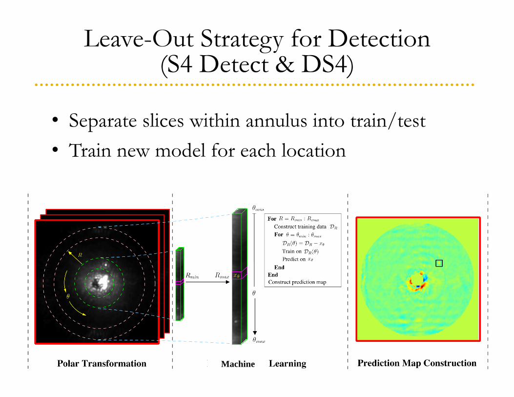
• Separate slices within annulus into train/test• Train new model for each location

Leave-Out Strategy for Detection (S4 Detect & DS4)

Machine

1. S4 Detect

[Fergus et al., Astrophysical Journal, under review]

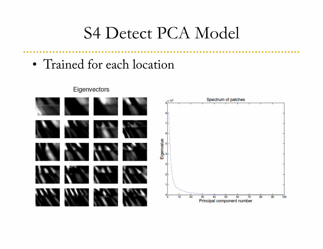
S4 Detect PCA Model

• Trained for each location

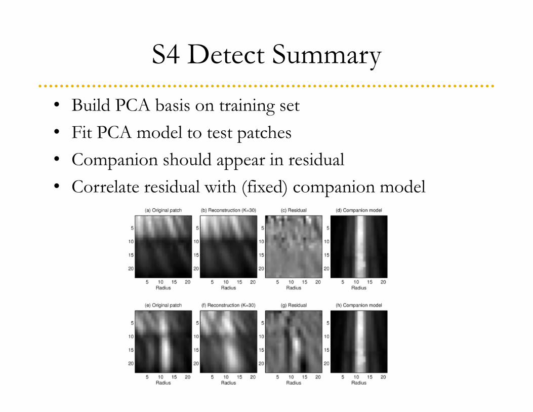
S4 Detect Summary • Build PCA basis on training set• Fit PCA model to test patches• Companion should appear in residual• Correlate residual with (fixed) companion model

2. DS4 Detect

[Fergus et al., Astrophysical Journal, under review]

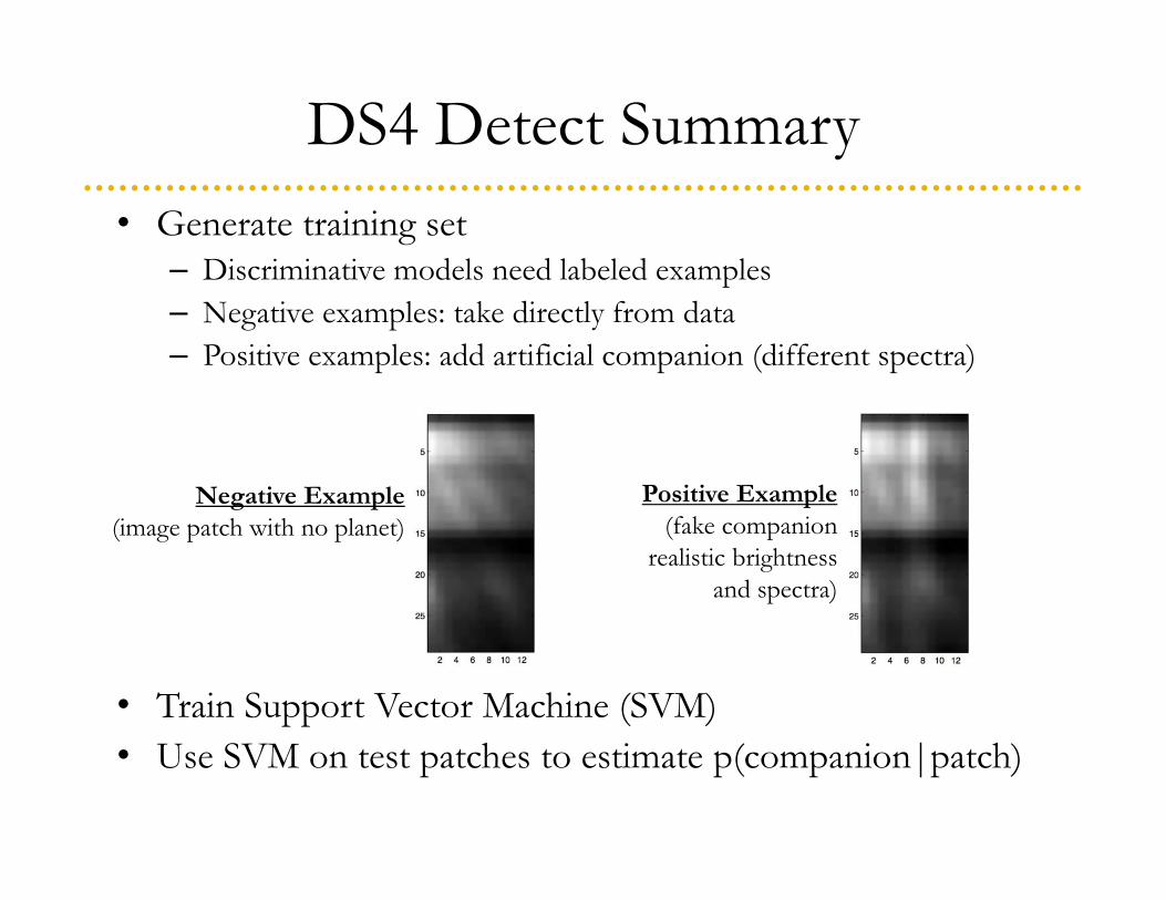
DS4 Detect Summary • Generate training set

– Discriminative models need labeled examples– Negative examples: take directly from data– Positive examples: add artificial companion (different spectra)

• Train Support Vector Machine (SVM) • Use SVM on test patches to estimate p(companion|patch)

Negative Example(image patch with no planet)

Positive Example(fake companion

realistic brightness and spectra)

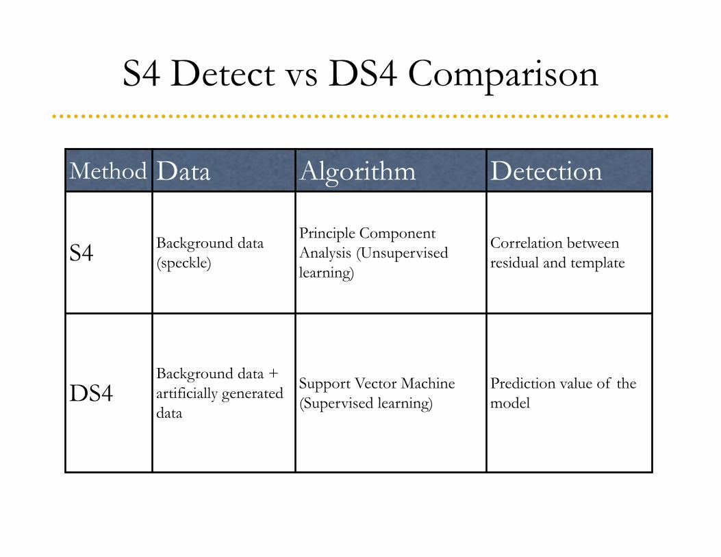
S4 Detect vs DS4 Comparison

Method Data Algorithm Detection

S4 Background data (speckle)

Principle Component Analysis (Unsupervised learning)

Correlation between residual and template

DS4Background data + artificially generated data

Support Vector Machine (Supervised learning)

Prediction value of the model

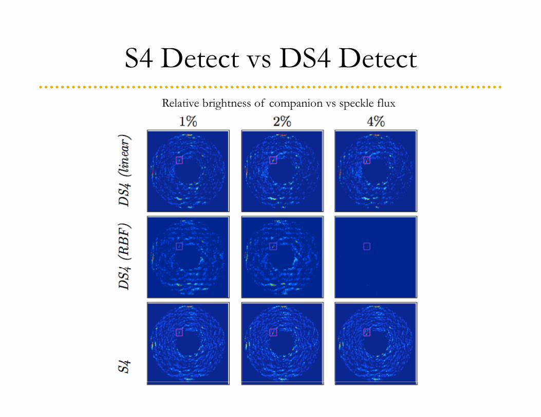
S4 Detect vs DS4 Detect Relative brightness of companion vs speckle flux

3. S4 Spectra

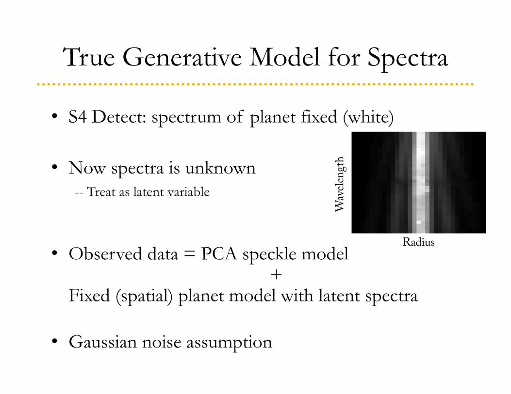
True Generative Model for Spectra

• S4 Detect: spectrum of planet fixed (white)

• Now spectra is unknown-- Treat as latent variable

• Observed data = PCA speckle model+

Fixed (spatial) planet model with latent spectra

• Gaussian noise assumption

Radius

Wav

elen

gth

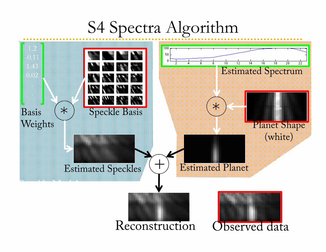
S4 Spectra Algorithm

Observed dataReconstruction

Estimated Speckles Estimated Planet

Speckle Basis

Estimated Spectrum

Planet Shape (white)

Radius

Wav

elen

gth

+

*Basis Weights

1.2-0.111.430.02

.

.

*

Speckle Model

PlanetModel

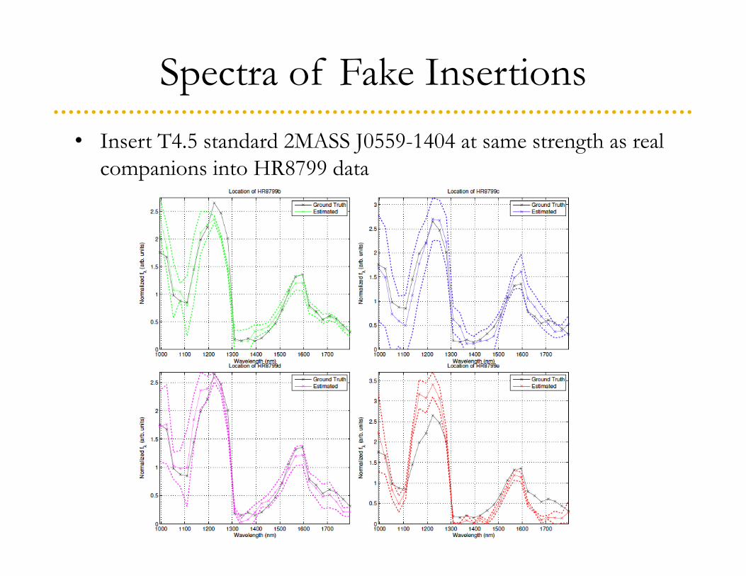
Spectra of Fake Insertions• Insert T4.5 standard 2MASS J0559-1404 at same strength as real

companions into HR8799 data

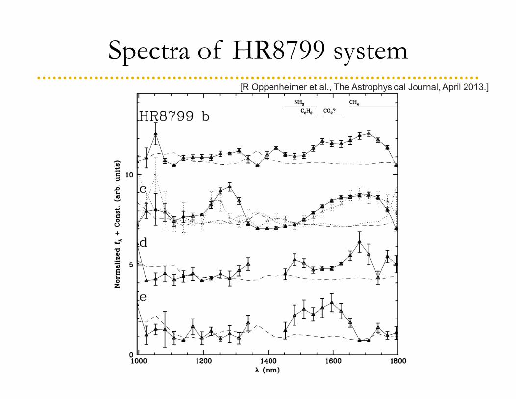
Spectra of HR8799 system[R Oppenheimer et al., The Astrophysical Journal, April 2013.]

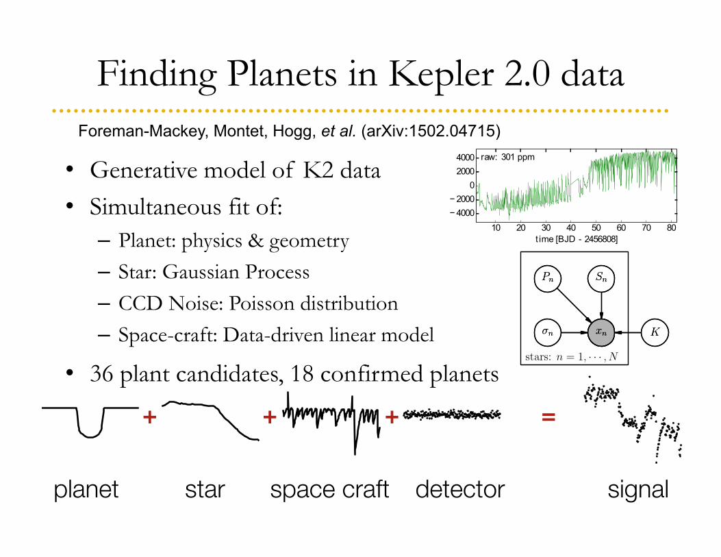
Finding Planets in Kepler 2.0 dataForeman-Mackey, Montet, Hogg, et al. (arXiv:1502.04715)

10 20 30 40 50 60 70 80t ime [BJD - 2456808]

− 4000− 2000

020004000 raw: 301 ppm

• Generative model of K2 data• Simultaneous fit of:

– Planet: physics & geometry– Star: Gaussian Process – CCD Noise: Poisson distribution– Space-craft: Data-driven linear model

• 36 plant candidates, 18 confirmed planets

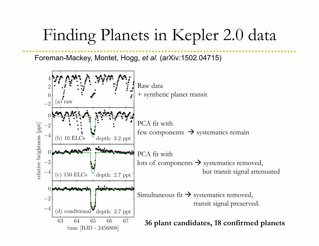
Finding Planets in Kepler 2.0 dataForeman-Mackey, Montet, Hogg, et al. (arXiv:1502.04715)

Raw data+ synthetic planet transit

PCA fit withfew components systematics remain

PCA fit withlots of components systematics removed,

but transit signal attenuated

Simultaneous fit systematics removed, transit signal preserved.

36 plant candidates, 18 confirmed planets

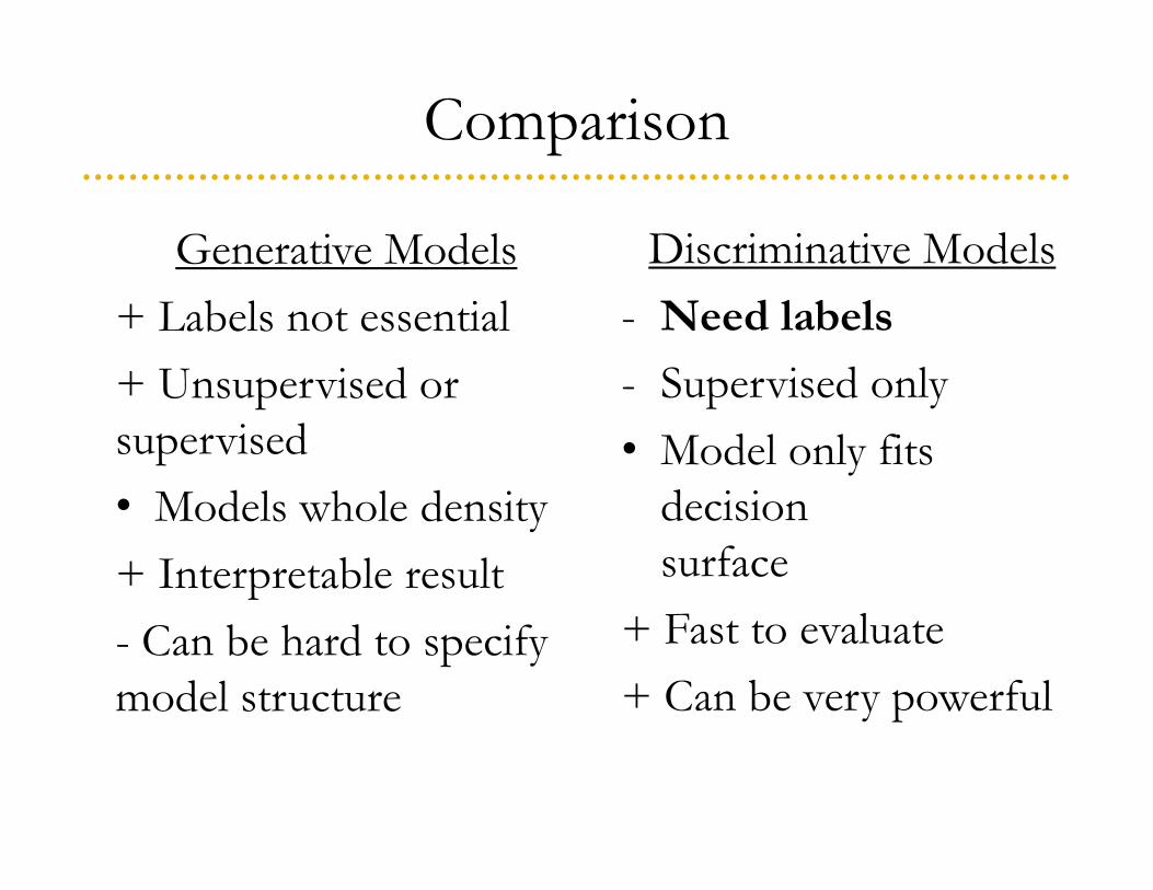
Comparison

Generative Models+ Labels not essential+ Unsupervised or supervised• Models whole density+ Interpretable result- Can be hard to specify model structure

Discriminative Models- Need labels

- Supervised only• Model only fits

decision surface

+ Fast to evaluate+ Can be very powerful

Final Thoughts

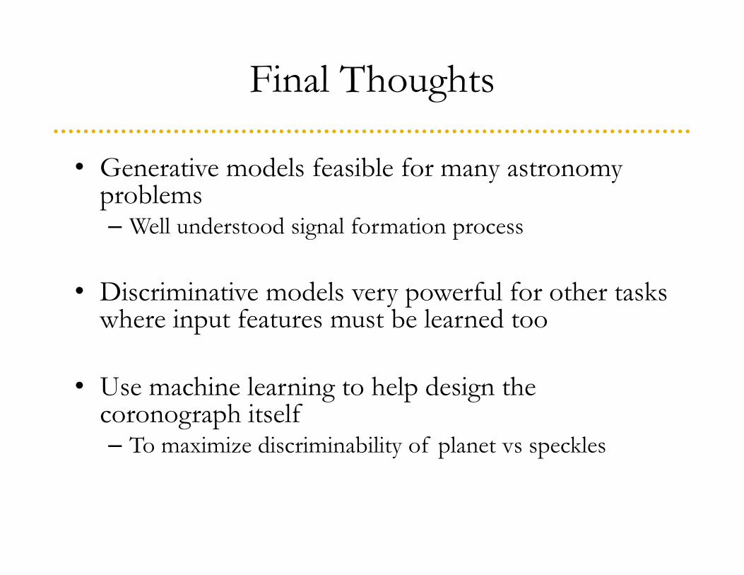
• Generative models feasible for many astronomy problems– Well understood signal formation process

• Discriminative models very powerful for other tasks where input features must be learned too

• Use machine learning to help design the coronograph itself– To maximize discriminability of planet vs speckles

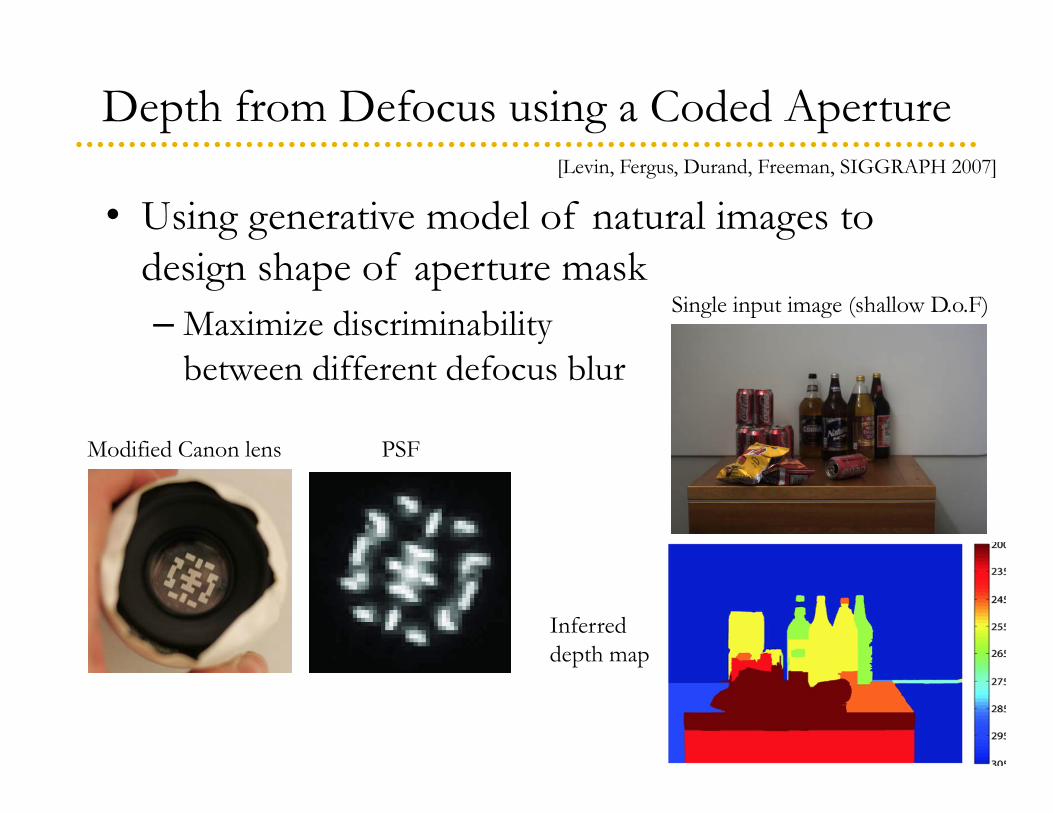
Depth from Defocus using a Coded Aperture

• Using generative model of natural images to design shape of aperture mask– Maximize discriminability

between different defocus blur

Modified Canon lens PSF

Single input image (shallow D.o.F)

Inferred depth map

[Levin, Fergus, Durand, Freeman, SIGGRAPH 2007]

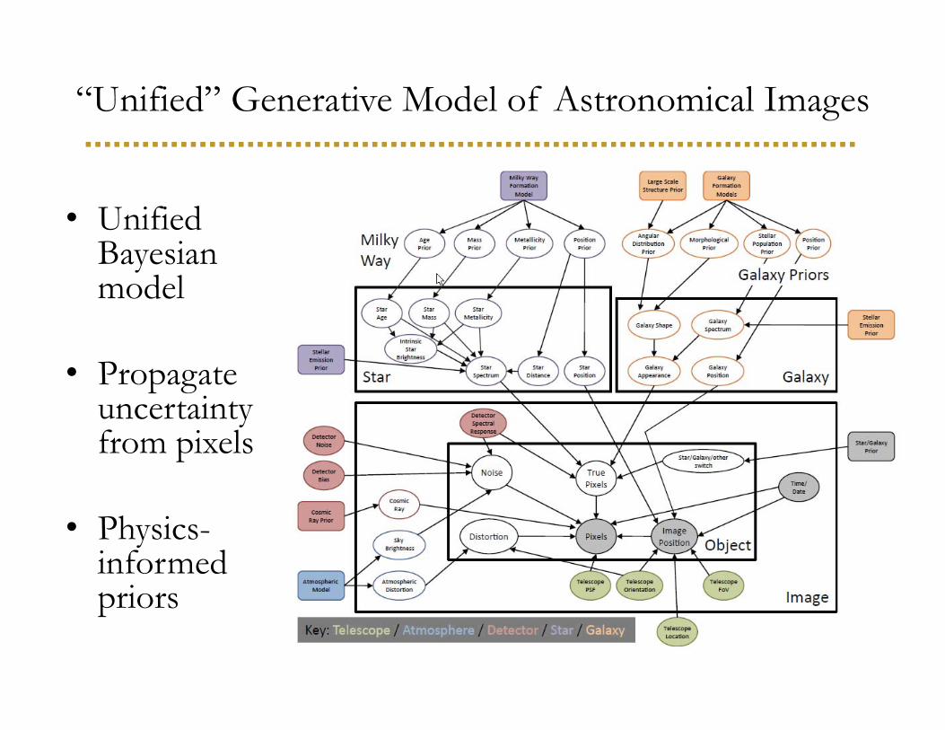
“Unified” Generative Model of Astronomical Images

• UnifiedBayesian model

• Propagateuncertaintyfrom pixels

• Physics-informedpriors

Hogg & Fergus, NSF #1124794 “CDI: A Unified Probabilistic Model of Astronomical Imaging”

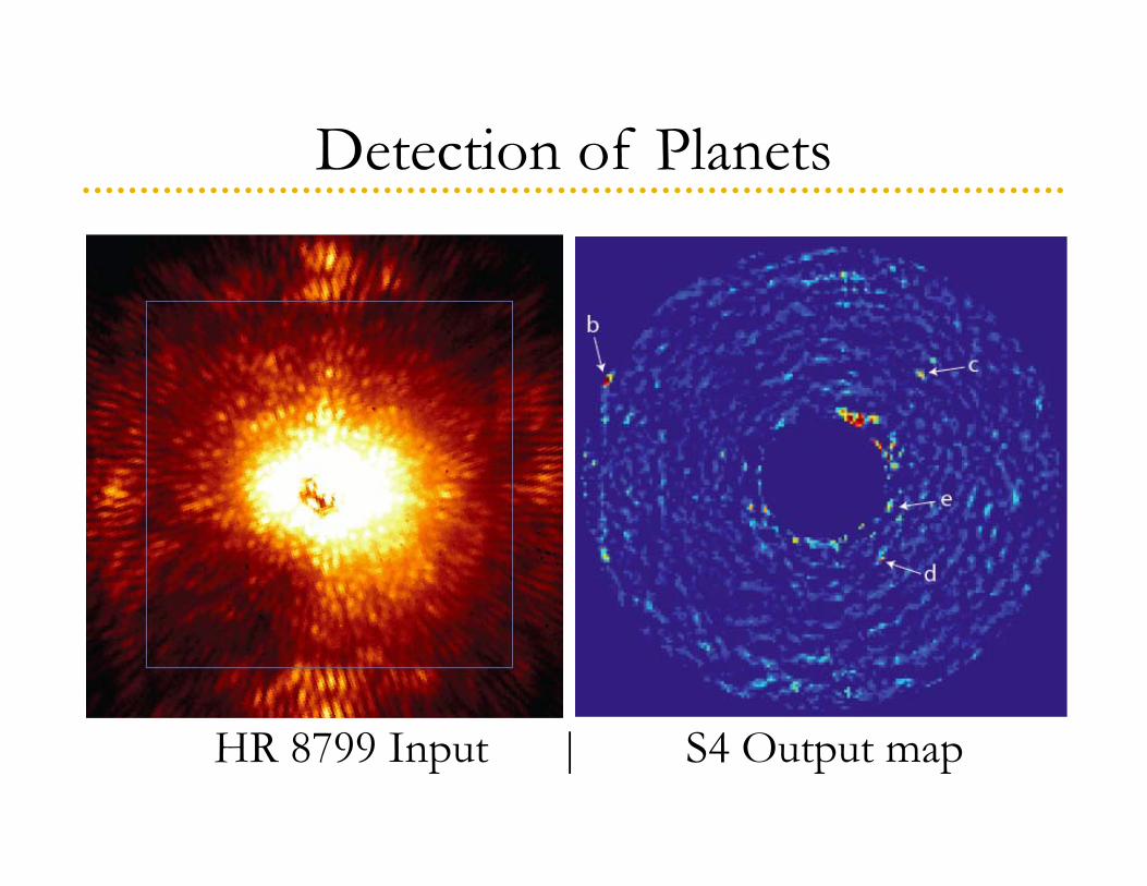
Detection of Planets

HR 8799 Input | S4 Output map

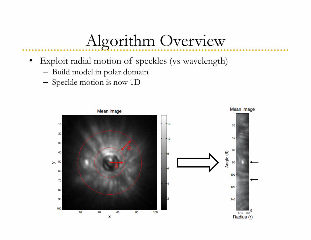
Algorithm Overview• Exploit radial motion of speckles (vs wavelength)

– Build model in polar domain– Speckle motion is now 1D

Joint Radius-Wavelength Model• Speckles are diagonal structures• Planet is vertical

– Key to separating the two• Assume: independence to

angle and exposure W

avel

engt

h

Wav

elen

gth

Wavelength

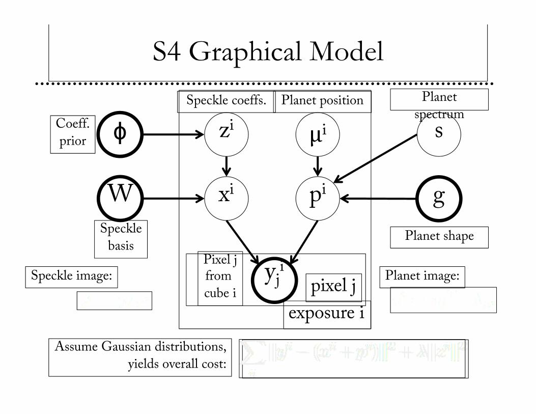
S4 Graphical Model

yji

pixel j

exposure i

xiW

zi

Speckle

basisPixel jfrom

cube i

Speckle coeffs.

s

pi

μi

g

Planet position

Planet shape

Planet

spectrum

ϕCoeff.

prior

Speckle image: Planet image:

Assume Gaussian distributions,

yields overall cost:

Approach

• Build statistical model of speckles– Physical model of optics too complex

• Few exposures of a given star (5-10)– Little data from which build model

• Need to exploit problem structure to yield more samples of speckles

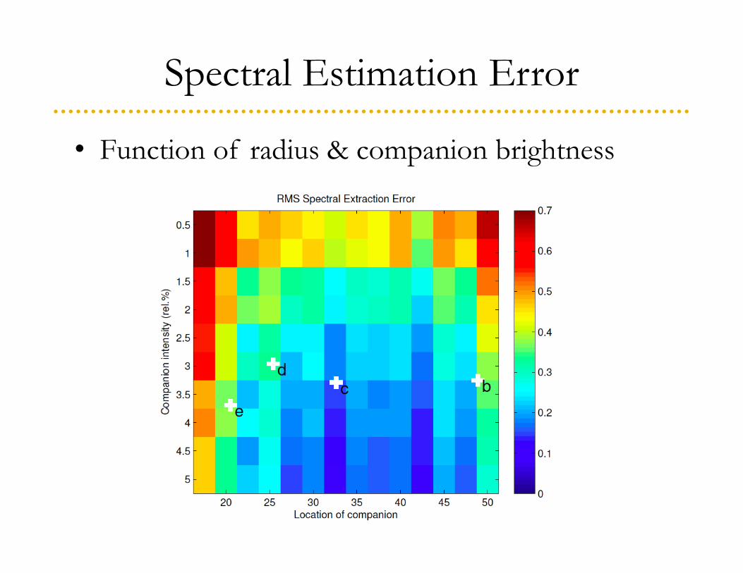
Spectral Estimation Error

• Function of radius & companion brightness

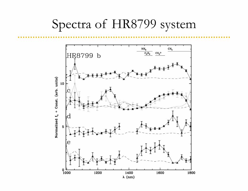
Spectra of HR8799 system

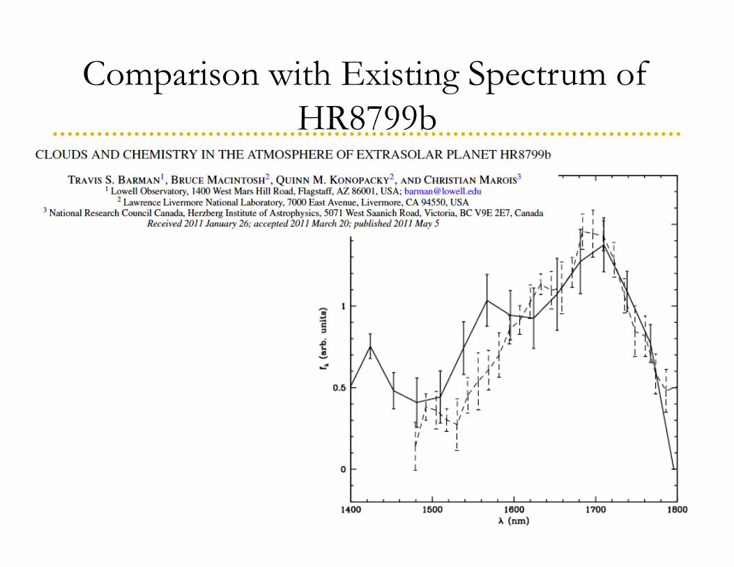
Comparison with Existing Spectrum of HR8799b

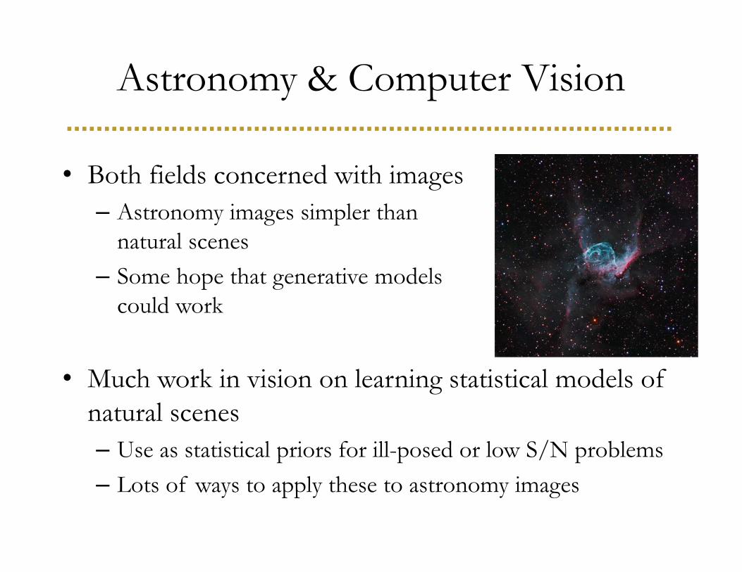
Astronomy & Computer Vision

• Both fields concerned with images– Astronomy images simpler than

natural scenes– Some hope that generative models

could work

• Much work in vision on learning statistical models of natural scenes– Use as statistical priors for ill-posed or low S/N problems– Lots of ways to apply these to astronomy images

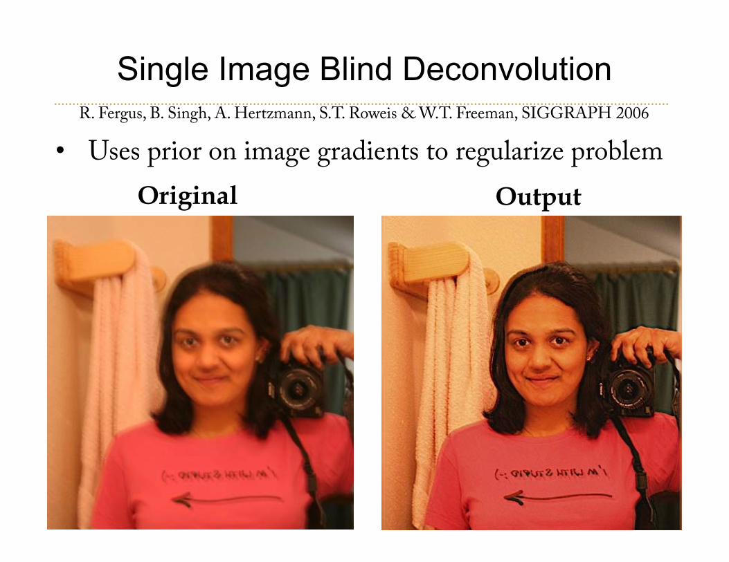
Single Image Blind Deconvolution

Original Output

R. Fergus, B. Singh, A. Hertzmann, S.T. Roweis & W.T. Freeman, SIGGRAPH 2006

• Uses prior on image gradients to regularize problem

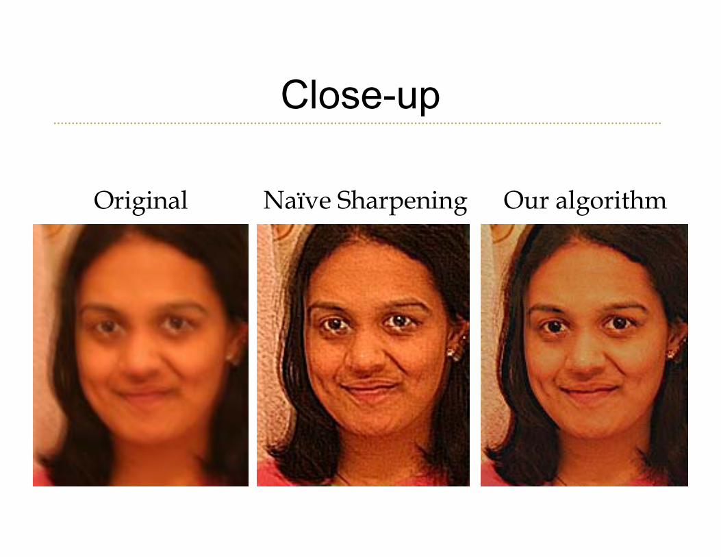
Close-up

Original Naïve Sharpening Our algorithm

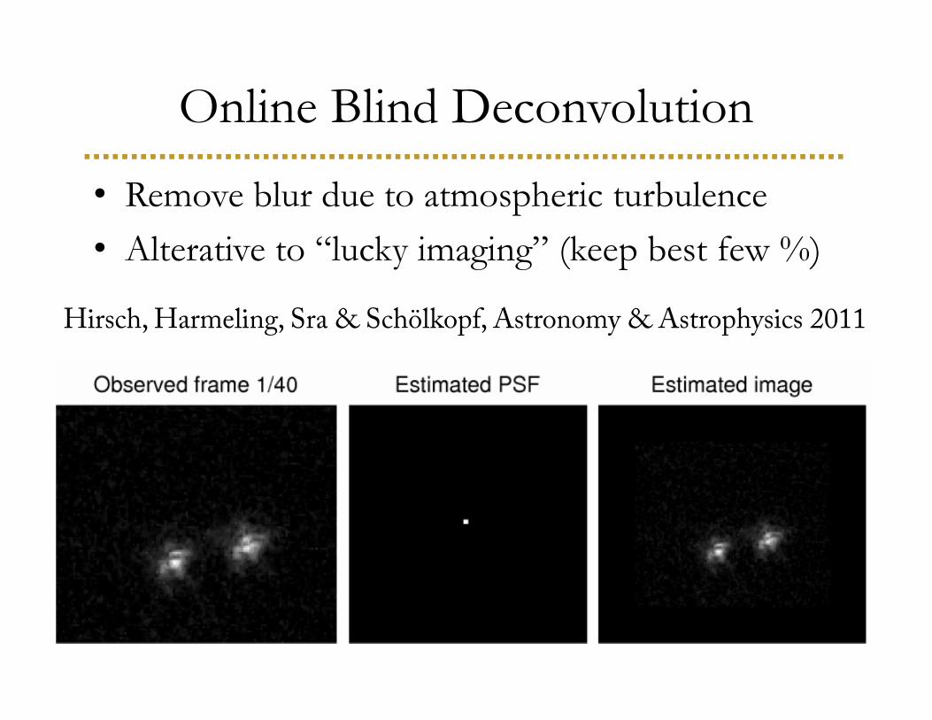
Online Blind Deconvolution

Hirsch, Harmeling, Sra & Schölkopf, Astronomy & Astrophysics 2011

• Remove blur due to atmospheric turbulence• Alterative to “lucky imaging” (keep best few %)

65

66

67

68

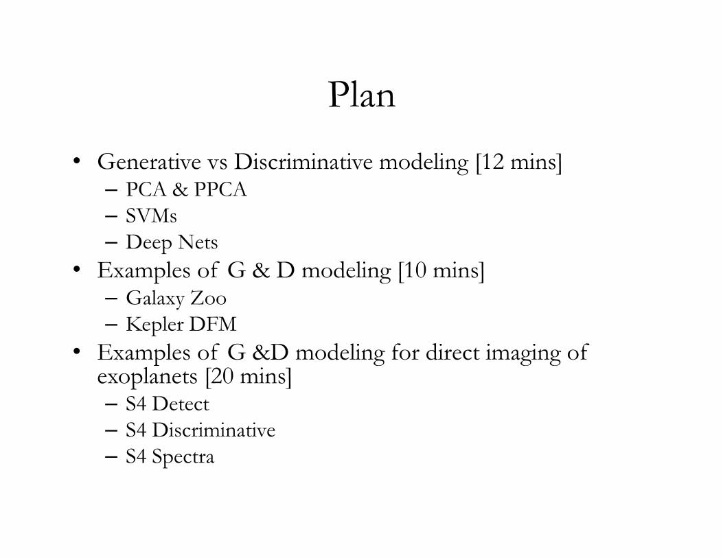
Plan• Generative vs Discriminative modeling [12 mins]

– PCA & PPCA– SVMs– Deep Nets

• Examples of G & D modeling [10 mins]– Galaxy Zoo– Kepler DFM

• Examples of G &D modeling for direct imaging of exoplanets [20 mins]– S4 Detect– S4 Discriminative– S4 Spectra

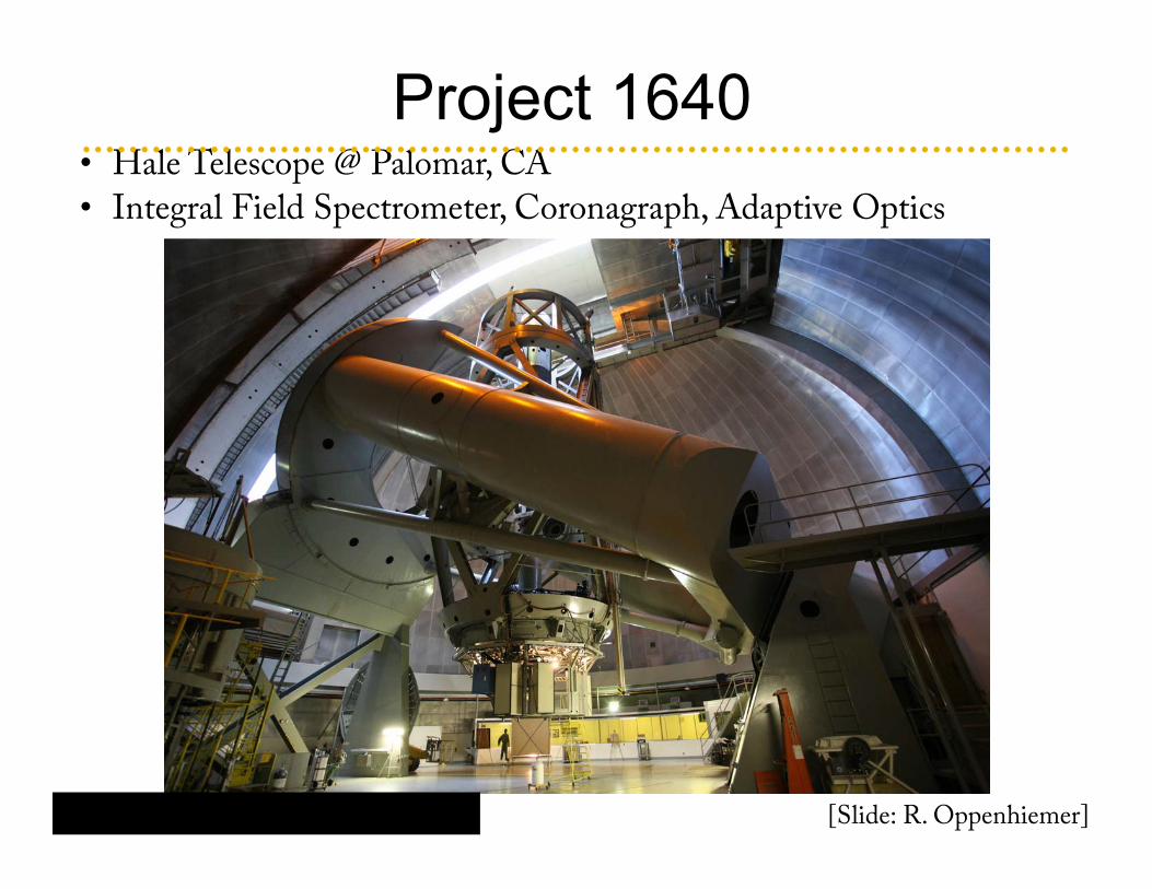
Project 1640

Hinkley et al. 2011c (PASP, 123, 74) [Slide: R. Oppenhiemer]

• Hale Telescope @ Palomar, CA

• Integral Field Spectrometer, Coronagraph, Adaptive Optics

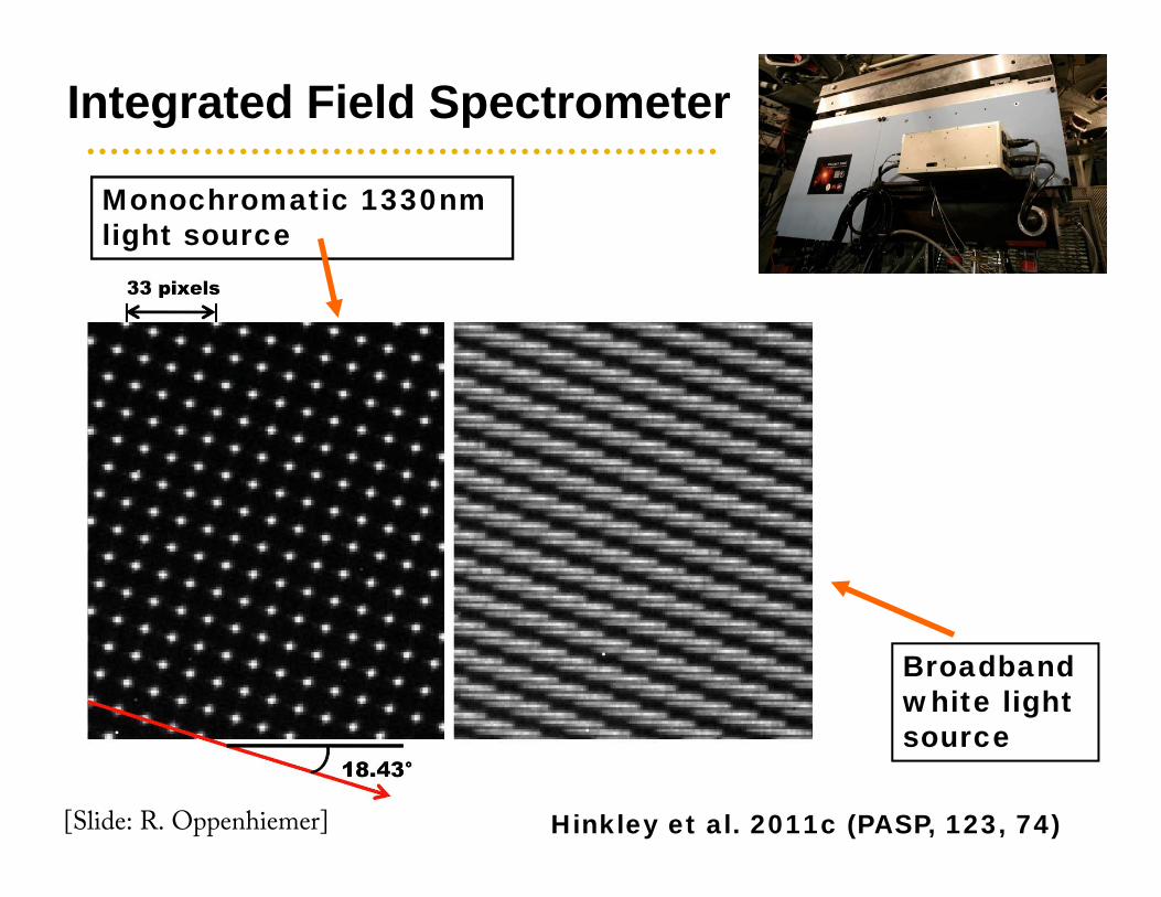
Integrated Field Spectrometer

Monochromatic 1330nm light source

Broadband white light source

Hinkley et al. 2011c (PASP, 123, 74)[Slide: R. Oppenhiemer]

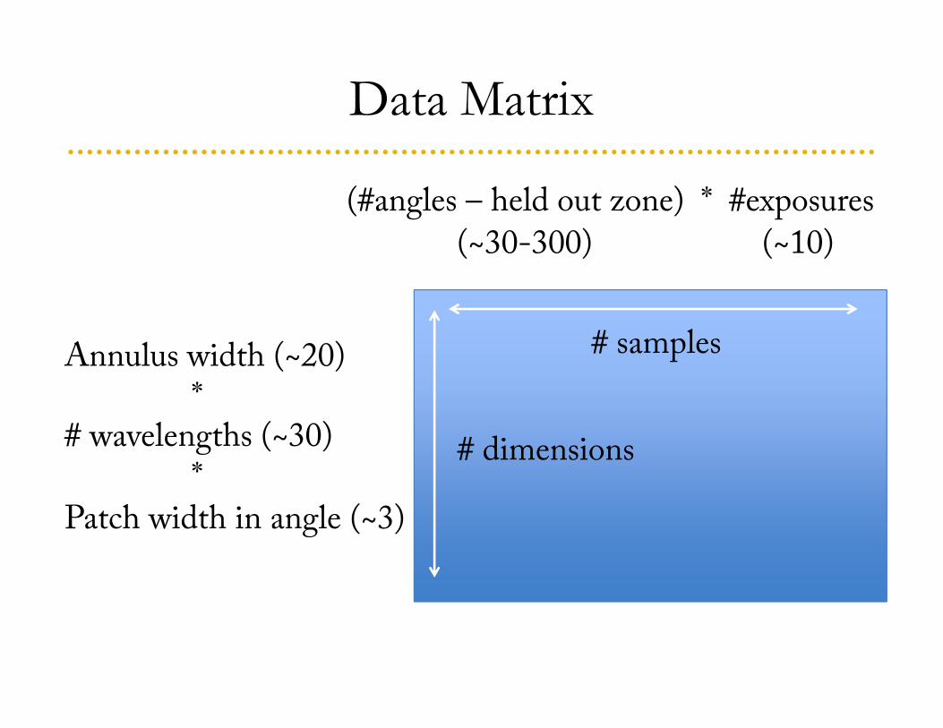
Data Matrix

Annulus width (~20) *

# wavelengths (~30) *

Patch width in angle (~3)

(#angles – held out zone) * #exposures

(~30-300) (~10)

# samples

# dimensions

Residual Error of PCA Model

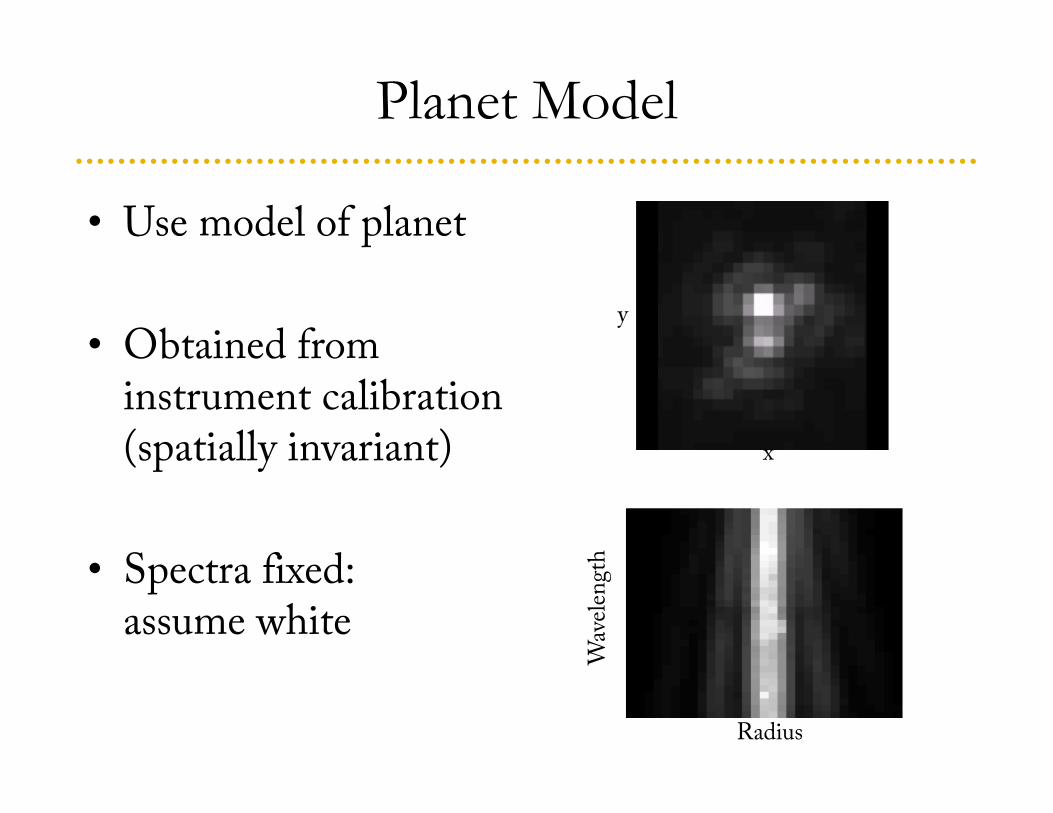
Planet Model

• Use model of planet

• Obtained from instrument calibration(spatially invariant)

• Spectra fixed:assume white

x

y

Radius

Wav

elen

gth

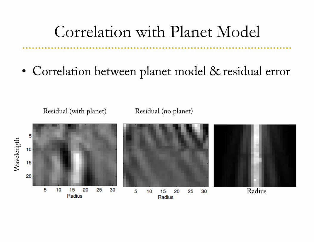
Correlation with Planet Model

• Correlation between planet model & residual error

Radius

Wav

elen

gth

Residual (with planet) Residual (no planet)

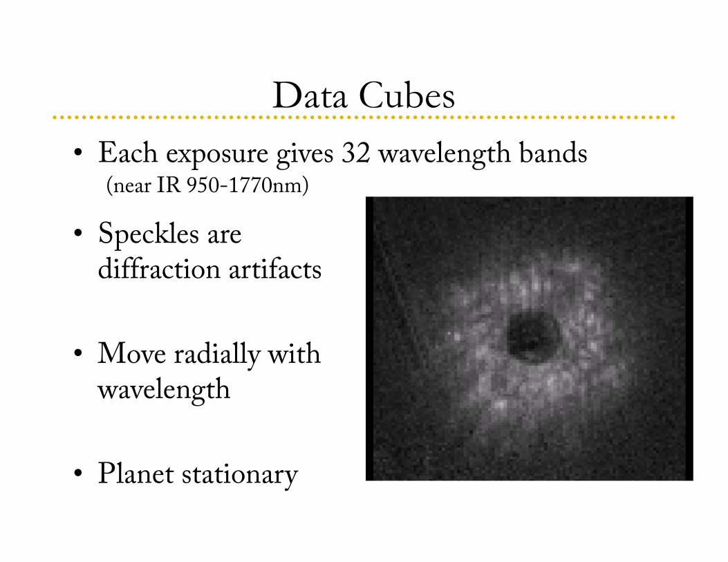
Data Cubes• Each exposure gives 32 wavelength bands

(near IR 950-1770nm)

• Speckles are diffraction artifacts

• Move radially with wavelength

• Planet stationary

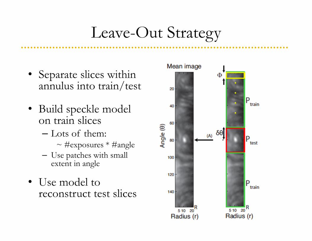
Leave-Out Strategy

• Separate slices withinannulus into train/test

• Build speckle model on train slices– Lots of them:

~ #exposures * #angle– Use patches with small

extent in angle

• Use model to reconstruct test slices

Evaluation

• 10 exposures of star HR8799 from June 2012

• Compare to leading astronomy algorithms:– LOCI (Local Combination Of Images)

Lafrenière et al. , The Astrophysical Journal, 660:770-780, May 2007

• Models speckles as linear combination of specklesfrom other wavelengths/exposures

– KLIP: Detection and Characterization of Exoplanets and Disks using Projections on Karhunen-Loeve Eigenimages, Remi Soummer et al., arXiv:1207.4197, July 2012

• PCA-based but does not exploit radius-wavelength structure

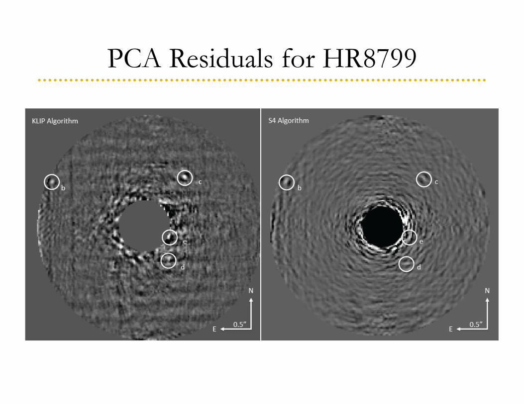
PCA Residuals for HR8799

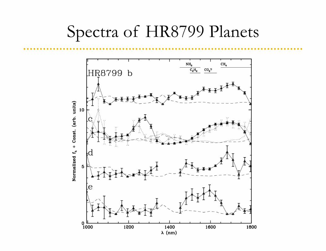
Spectra of HR8799 Planets