Embed Size (px)
Citation preview
University of Amsterdam
Faculty of Science
Program of Computational Science
Machine Learning Classifications for ThePrediction of Intraday Trading Signal
Wentao Yang
Supervisor: Prof. Dr. Drona Kandhai
Submitted in part fulfillment of the requirements for the degree ofMaster of Science in Computational Science of the University of Amsterdam , November 6,
2017

Abstract
This paper proposes and studies a series of Machine learning methods to make prediction for
intraday trading signal, by using different combinations of stock market technical indicators
as the feature set (the input) into the classier. The main purpose of this paper is to do
research on existing study on application of Machine Learning Classification Algorithms in
automatic quantitative trading, and further uses and combines multiple techniques into one
two-layers filter system to help the automatic trading algorithm in the system with better
financial market information analytical ability and more reliable trading decision making. The
techniques we investigate include famous Machine Learning classifiers such as Artificial Neural
Network, Random Forest, and we also apply re-sampling methods to reduce the imbalanced
problem in the dataset. In total, 1 Year pre-processed dataset from Japanese stock market
(Nikkei) is used to train and test the classification algorithms. As to the evaluation of different
algorithms, the confusion matrix is applied to calculate the evaluation metrics such as accuracy
and precision. Furthermore, due to the imbalanced class problem in the dataset, Kappa and
AUC are employed to measure and compare the performance of the filters based on different
combination of machine learning classification algorithms. Lastly the effect of filter (classier)
on the profitability of trading strategy is also examined.
The findings show that the profitability of momentum trading based strategy/algorithms can
be significantly improved with the help of machine learning applications. With the strong
power of machine learning algorithms in high-dimensional data analysis, the filter can improve
the ability of strategy in better analyzing the trend and relationship in the intraday market by
using the tremendous intraday market data, and improve trading decision making based on the
signal from the filter system.
i

ii

Acknowledgements
This master thesis marks the end of my master study at University of Amsterdam. The work
has at times been challenging, but it has also been very useful and rewarding for my future
career development at the same time. I would like to express my feelings to:
• My colleagues at Algorithmic Trading Group. Thanks to them, I got the opportunity
to do my master project in the firm and gain a lot experience of applying quantitative
techniques in financial algorithmic trading. I appreciate their supports and practical
suggestions regarding the trading strategy during my research.
• My Supervisor and researchers in the Computational Finance Group at UvA. I’d like to
say thanks to them for their kind understandings about my special situation at the last
stage of my study, and of course for their valuable inputs and suggestions during the
writing process.
• Finally, I’d like to say my love and thanks to my girlfriend. Your confidence and support
in me has been a constant in my life, in the meantime your love and patience has been
the foundations of this work.
iii

iv
Contents
Abstract i
Preface iii
1 Introduction 1
1.1 Relevant Studies on Machine learning in Finance . . . . . . . . . . . . . . . . . 2
1.2 Structure of Paper . . . . . . . . . . . . . . . . . . . . . . . . . . . . . . . . . . 4
2 Literature Study on Machine Learning 5
2.1 Overview . . . . . . . . . . . . . . . . . . . . . . . . . . . . . . . . . . . . . . . . 5
2.2 Machine Learning Algorithms . . . . . . . . . . . . . . . . . . . . . . . . . . . . 6
2.3 Supervised Learning Classification Algorithms . . . . . . . . . . . . . . . . . . . 7
2.3.1 Support Vector Machine Algorithm (SVM) . . . . . . . . . . . . . . . . . 7
2.3.2 Artificial Neural Network Algorithm (ANN) . . . . . . . . . . . . . . . . 8
2.3.3 Random Forest Algorithm (RF) . . . . . . . . . . . . . . . . . . . . . . . 10
2.3.4 Xgboost . . . . . . . . . . . . . . . . . . . . . . . . . . . . . . . . . . . . 11
2.3.5 Model Stacking: Combing Classifiers . . . . . . . . . . . . . . . . . . . . 12
v
vi CONTENTS
2.4 Evaluation metrics . . . . . . . . . . . . . . . . . . . . . . . . . . . . . . . . . . 13
2.4.1 Confusion matrix and accuracy . . . . . . . . . . . . . . . . . . . . . . . 13
2.4.2 Precision, Recall and F1-Score . . . . . . . . . . . . . . . . . . . . . . . . 15
2.4.3 Kappa . . . . . . . . . . . . . . . . . . . . . . . . . . . . . . . . . . . . . 16
2.4.4 ROC and AUC . . . . . . . . . . . . . . . . . . . . . . . . . . . . . . . . 17
2.4.5 Performance of Profitability of the model . . . . . . . . . . . . . . . . . . 17
2.5 Model Validation . . . . . . . . . . . . . . . . . . . . . . . . . . . . . . . . . . . 20
2.5.1 Holdout . . . . . . . . . . . . . . . . . . . . . . . . . . . . . . . . . . . . 20
2.5.2 K-fold Cross-Validation . . . . . . . . . . . . . . . . . . . . . . . . . . . . 21
2.6 Summary . . . . . . . . . . . . . . . . . . . . . . . . . . . . . . . . . . . . . . . 22
3 Project Design and Data Engineering 24
3.1 Project Description . . . . . . . . . . . . . . . . . . . . . . . . . . . . . . . . . . 24
3.2 Architecture of the Filter . . . . . . . . . . . . . . . . . . . . . . . . . . . . . . . 25
3.3 Trading Data Description and Engineering . . . . . . . . . . . . . . . . . . . . . 27
3.3.1 Data Description . . . . . . . . . . . . . . . . . . . . . . . . . . . . . . . 27
3.3.2 Data Pre-Processing . . . . . . . . . . . . . . . . . . . . . . . . . . . . . 30
3.3.3 Feature Engineering . . . . . . . . . . . . . . . . . . . . . . . . . . . . . 32
3.3.4 Feature Reduction . . . . . . . . . . . . . . . . . . . . . . . . . . . . . . 33
3.3.5 Imbalanced Data and Solutions . . . . . . . . . . . . . . . . . . . . . . . 37
3.4 Performance and Efficiency . . . . . . . . . . . . . . . . . . . . . . . . . . . . . . 39

4 Experiments and Outputs 41
4.1 Layer 1: Profit Margin Prediction . . . . . . . . . . . . . . . . . . . . . . . . . . 42
4.1.1 Imbalanced Data . . . . . . . . . . . . . . . . . . . . . . . . . . . . . . . 42
4.1.2 Balanced Data . . . . . . . . . . . . . . . . . . . . . . . . . . . . . . . . 46
4.2 Layer 2: Movement Direction Prediction . . . . . . . . . . . . . . . . . . . . . . 52
4.3 Performance of Combining Two Layers . . . . . . . . . . . . . . . . . . . . . . . 53
5 Conclusion 55
5.1 Summary of Thesis Achievements . . . . . . . . . . . . . . . . . . . . . . . . . . 56
5.2 Future Work . . . . . . . . . . . . . . . . . . . . . . . . . . . . . . . . . . . . . . 57
Bibliography 57
6 Appendix 63
vii

viii

List of Tables
2.1 Confusion Matrix: 2 Classes Problem . . . . . . . . . . . . . . . . . . . . . . . . 14
2.2 Confusion Matrix: Basic Trading Example . . . . . . . . . . . . . . . . . . . . . 16
4.1 Experiment Outputs (Test Set): Imbalanced Data with all features . . . . . . . 43
4.2 Experiment Outputs (Test Set): Imbalanced Data with PCA feature reduction . 44
4.3 Experiment Outputs (Test Set): Imbalanced Data with selected Feature . . . . . 45
4.4 Experiment Outputs (Test Set): balanced Data (ENN) with all feature . . . . . 47
4.5 Experiment Outputs (Test Set): balanced Data (SMOTE) with all feature . . . 47
4.6 Experiment Outputs (Test Set): balanced Data (SMOTEENN) with all feature . 47
4.7 Experiment Outputs (Test Set): balanced Data (ENN) with PCA feature reduction 48
4.8 Experiment Outputs (Test Set): balanced Data (SMOTE) with PCA feature
reduction . . . . . . . . . . . . . . . . . . . . . . . . . . . . . . . . . . . . . . . 49
4.9 Experiment Outputs (Test Set): balanced Data (SMOTEENN) with PCA fea-
ture reduction . . . . . . . . . . . . . . . . . . . . . . . . . . . . . . . . . . . . . 49
4.10 Experiment Outputs (Test Set): balanced Data (ENN) with selected feature . . 50
4.11 Experiment Outputs (Test Set): balanced Data (SMOTE) with selected feature 51
ix

4.12 Experiment Outputs (Test Set): balanced Data (SMOTEENN) with selected
feature . . . . . . . . . . . . . . . . . . . . . . . . . . . . . . . . . . . . . . . . . 51
4.13 Experiment Outputs (Test Set): Layer-2 . . . . . . . . . . . . . . . . . . . . . . 52
4.14 Experiment Outputs (Test Set): Combining Layer-1 and Layer-2 . . . . . . . . . 54
4.15 Profit Composition (10% of dataset with in total 18291 sample trades) . . . . . 54
6.1 Example Trade . . . . . . . . . . . . . . . . . . . . . . . . . . . . . . . . . . . . 63
6.2 Feature Table . . . . . . . . . . . . . . . . . . . . . . . . . . . . . . . . . . . . . 64
x
List of Figures
2.1 Unsupervised Learning: Clustering . . . . . . . . . . . . . . . . . . . . . . . . . 6
2.2 Example of Support Vector Machine (SVM) Classification . . . . . . . . . . . . 8
2.3 Structure of Artificial Neural Network . . . . . . . . . . . . . . . . . . . . . . . . 9
2.4 A Neural Network node . . . . . . . . . . . . . . . . . . . . . . . . . . . . . . . 10
2.5 Example of Random Forest . . . . . . . . . . . . . . . . . . . . . . . . . . . . . 11
2.6 Structure of Xgboost . . . . . . . . . . . . . . . . . . . . . . . . . . . . . . . . . 12
2.7 Diagram of Model Stacking . . . . . . . . . . . . . . . . . . . . . . . . . . . . . 13
2.8 ROC Curve . . . . . . . . . . . . . . . . . . . . . . . . . . . . . . . . . . . . . . 18
2.9 General Trading Structure/Process . . . . . . . . . . . . . . . . . . . . . . . . . 19
2.10 Holdout Validation . . . . . . . . . . . . . . . . . . . . . . . . . . . . . . . . . . 21
2.11 Process of 10-fold Cross Validation . . . . . . . . . . . . . . . . . . . . . . . . . 22
3.1 Diagram of The Trading System (Example) . . . . . . . . . . . . . . . . . . . . 27
3.2 Histogram of Features . . . . . . . . . . . . . . . . . . . . . . . . . . . . . . . . 28
3.3 Descriptive Statistics . . . . . . . . . . . . . . . . . . . . . . . . . . . . . . . . . 29
3.4 Histogram of Scaled Features . . . . . . . . . . . . . . . . . . . . . . . . . . . . 31
xi
3.5 Histogram of Target Variables . . . . . . . . . . . . . . . . . . . . . . . . . . . . 33
3.6 Histogram of New Feature: A20 . . . . . . . . . . . . . . . . . . . . . . . . . . . 34
3.7 Correlations Plot . . . . . . . . . . . . . . . . . . . . . . . . . . . . . . . . . . . 35
3.8 Principal Component Analysis (PCA) for Group 1(The Layer 1) Plot . . . . . . 36
3.9 Embedded Feature Selection . . . . . . . . . . . . . . . . . . . . . . . . . . . . . 36
3.10 Histogram of Target Variable-Size after over-/under-sampling. . . . . . . . . . . 38
3.11 Histogram with SMOTENN re-sampling method . . . . . . . . . . . . . . . . . . 39
4.1 Imbalanced Data (Test Set): Feature Importance Plot . . . . . . . . . . . . . . . 45
xii
Chapter 1
Introduction
Forecasting the financial securities especially the cash equity, has been widely studied by many
researchers and financial firms in the past decade. Although many results have been published in
books and papers, some of them are rarely applicable and repeatable in real financial problems
for some reasons. Nowadays, as the market has been shifted from traditional (manual) trading
to a more modern and automated electronic trading, recent research now put more and more
focus on the application of different quantitative methods in high-frequency trading (HFT)
data (by seconds/minutes, instead of day or week). However, there might be some difficulties
in dealing with HFT data, for example, extremely large quantities of trading data and relatively
long processing time by the model to compute a prediction comparing to the limited time for
determination a trader has.
When talking about the stock prediction, the first thing comes out is the important theory in
financial economics -Efficient Market Hypothesis (EMH) by Fama in the 1965[1], which states
that the current asset’s price reflects all known information, thus only new information can
lead to a move in the price. As we know, there are three common methods for the stock
market prediction that used by financial industry, namely the fundamental analysis, technical
analysis and quantitative analysis, where both employs relevant information to make movement
prediction although the analytical methods are different.
1
2 Chapter 1. Introduction
The fundamental analysis examines both macroeconomic and microeconomics factors, which in-
cludes elements such as the health of a country economy or global economy, quarterly/annually
company financial report, competitor performance and the corresponding market situation. By
doing fundamental research on these factors, an investor can obtain a general overview of the
company/industry and then determine a fair value (stock price) for the business. For example,
if the company (stock price) is undervalued according to the research result, then we can buy
the stock to make profit.
The idea of traditional technical analysis is to anticipate what other participants in the market
are thinking by using historical market data, mainly based on the stock price and trading
volume. With the help of mathematical/statistical model, we can use historical data to predict
future movements in the stock price, by identifying the trend of price movement and extracting
and inspecting the pattern visually from noisy data. Therefore, trading decision can be made
on the basis of the prediction.
1.1 Relevant Studies on Machine learning in Finance
In the past 10 years, trading gradually became a more and more complex which made the
market keep getting faster and the volumes of trading data keep escalating. Furthermore, the
market also became more volatile, as a result some huge and unexpected shifts may occur in
the market, such as what it could be found in 2007-2009 financial crisis. For old methods as
mentioned above, they have difficulty in processing large volume data and thus not be able to
make quick and correct predictions for those unexpected sudden shifts, but these two factors
are the most important things for high-frequency trading firms.
Recent developments in computing technology and data science has made traditional technical
analysis into a more quantitative approach. Techniques such as machine learning offer the
potential to improve short-term prediction for market movements or key variables, even during
volatile markets, because they can incorporate a much wider range of factors in their models,
1.1. Relevant Studies on Machine learning in Finance 3
and due to their high efficiency in computing. Prediction, as the most commonly used ap-
plication based on machine learning in financial area, there are many existing researches and
literature regarding this topic. Huang and Tsai [3] presents their hybrid-methods by combining
traditional technical analysis and artificial neural network for stock market prediction, where
the neural network classifier is mainly used for feature selection. Similarly, Wu et al.[4] also
use a radial basis function neural network model for stock index prediction, where the model
is optimized heuristically by artificial fish swarm algorithm. In 2013, Menconi and Gori[5]
uses support vector machine to balance recall and precision in stock market predictors, and by
using the selected indicators they make a profitable model with the help of technical analysis.
There are also researches about comparison of performance of different algorithms in stocking
trend prediction, for example Salim, compares between the performance of Probabilistic neural
network (PNN) and SVM and finds out that the PNN performs the best when only technical
indicators are used.
In addition to the prediction task, there are another two types of application based on machine
learning in financial trading, namely finding relationship/association and generating trading
strategies. For instance, Kapoor and Khurana [26] presents their idea about using Genetic
Algorithms in designing and building technical trading system. Wang[22] uses quantitative
methods to find the intraday inefficiency between the heating and natural gas markets.
However, it should be pointed out that none of researchers above claim that their prediction
model can work in real-time settings because their data source are mostly daily data instead
of high-frequency data. For those successful models or applications who can work in real-time
trading environment, there are also no incentive for the researchers or sponsoring firms to pub-
lish results. In fact, quantitative trading firms or researchers do not only use this quantitative
analysis for price prediction, but now also for the area of trading/hedging strategy development,
risk management and portfolio optimization. The example applications of quantitative method
can be algorithmic trading, statistical arbitrage and electrical market marking, where the main
purpose of using the quantitative methods is to replace the human element in trading with a
more technical and automatic way, which are commonly used in HFT firms.

4 Chapter 1. Introduction
1.2 Structure of Paper
The main goal of this research is to build a real-time filter system for trading algorithms that
used in Algorithmic Trading Group (ATG), the Netherlands, in order to improve the overall
performance of the strategy in term of profitability. To be precise, there are two layers in
the filter, where the first layer is to predict the profit margin of potential trade while at the
second layer we explore the predictability of market movement direction of the chosen stock
from previous layer, by employing the machine learning classification algorithms with different
set of technical market features. In this research, we use one-year data from Japanese cash
equity market with in total 23 intraday markets features, such as bid-ask spread, one-minute
trading volume and history volatility.
In the following, Chapter 2 will discuss a literature study of machine learning in general, such
as the introduction to the supervised machine learning algorithms that used in this research,
evaluation metrics for comparing the performance of different classifiers and lastly the model
validation. A description of project, framework of filter system, pre-data engineering and
resampling techniques will be involved in the Chapter 3, The Chapter 4 will present the results
of different classifiers with using different types of modified dataset in term of both statistical
performance, and the one with best performance is selected to further examine its impacts on
the profitability of trading strategy. Lastly, we will summarize and give suggestions for future
improvement.

Chapter 2
Literature Study on Machine Learning
2.1 Overview
Because of breakthroughs in both technology and computing algorithms, the trading industry
has shifted from a traditional manual trading to a more technology- and data-driven automated
trading. There are now many different quantitative techniques that can used to predict the
stock market movements, but as noted most of published studies don’t work in real-time setting
with using medium- or high-frequency data. The reason for the lack of published results in real-
time application can be simply be that there is little incentive to publish such (good) methods
in academic literature for either researchers or trading firms. The incentive for researchers to
instead sell them to a trading firm is much greater than publish their findings, monetarily.
Similarly, for those trading firms who build good model to predict the stock movement, they
have no incentive to share the model with other competitors neither. This is the goal of
this research, to explore the application of modern quantitative algorithms, namely Machine
Learning, in predicting the intraday stock movement.
In this chapter, the discussion mainly covers what machine learning is and how we can apply the
algorithm from machine learning to learn from data. In the Section 2.2 and 2.3, an overview of
popular algorithms from machine learning is given, such as Support Vector Machine (SVM) and
5
6 Chapter 2. Literature Study on Machine Learning
Random Forest (RF). Section 2.4 examines different methods for evaluating the performance
of different algorithms by using the confusion metrics. In the section 2.5, a review on model
validation method will be given.
2.2 Machine Learning Algorithms
As part of artificial intelligence, machine learning employs algorithms to explore the pattern
in data and make forecasts about future events. There are two types of Machine Learning
Algorithm, namely the unsupervised learning algorithms and supervised learning algorithms.
The key difference between supervised learning and unsupervised learning is that the output
variable (target) are provided for the supervised one in order to train the machine and desired
output, while in the unsupervised learning modelling it does not include target variable because
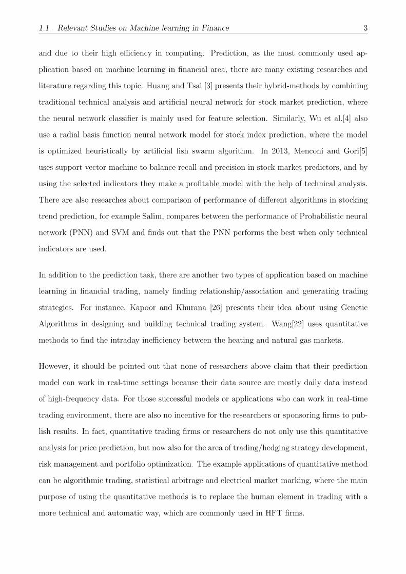
the main aim is to find the similarity among the groups. For instance, clustering is one example
of an unsupervised learning methods as showed in the two-dimensional demonstration below.
It can be seen that the data was clustered into 3 groups, but it can also be partitioned into 2
cluster in this case. In general, for clustering problems, the “right” number of cluster depends
on prior knowledge that used to determine the degree of similarity for the underlying problem.
Figure 2.1: Unsupervised Learning: Clustering
According to the problem characteristics and the data source available, we can choose between
2.3. Supervised Learning Classification Algorithms 7
supervised and unsupervised learning algorithms. In this research, since the target is known
which is the direction of intraday stock movement, namely go long or go short, the supervised
learning algorithm should be used. Furthermore, as the type of target attribute is discrete
instead of continuous, the classification algorithms is applied. Therefore, in the next section
we explore different classification learning algorithms from supervised techniques, since the
performance of different algorithms may differ due to the characteristics of underlying dataset.
2.3 Supervised Learning Classification Algorithms
Classification as one of the Machine Learning techniques, does analysis on a given dataset, then
takes each instance of the dataset, and lastly assigns the instance to a particular class where
the corresponding classification error will be the smallest. As similar to other machine learning
algorithms, the whole process of classification has two steps, at the step one the classification
model is trained based on the training dataset, and then in the next step the training model
is applied to test against the test dataset in order to measure the corresponding performance
and accuracy. The final goal pf classification is to assign class label for the dataset whose class
label is not known.
In the following, a short discussion regarding the classification algorithms that applied in this
research will be given.
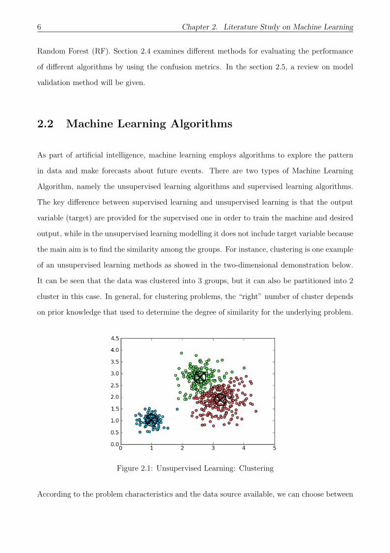
2.3.1 Support Vector Machine Algorithm (SVM)
Support Vector Machines (SVM) were first introduced to solve the pattern classification and
regression problems by Vapnik and his colleagues in 1995 [8]. Originally, a SVM classifier are
designed for two-class problem the binary object by looking the plane which can separate two
types of object optimally. However, it now can work in multiple classes problem by multiple
binary classifications between each pair of classes.
8 Chapter 2. Literature Study on Machine Learning
To be specific, the classifier mostly uses a linear function[8] of the feature to classify the ob-
servation. The margin nearby the linear separation area is computed, which should be as large
as possible. For higher dimensional space, a higher dimensional partition is done by non-linear
function which can be applied with the help of kernel in support vector machine function in
python, such as radial basis function (rbf) and polynomial (’poly’).
Figure 2.2: Example of Support Vector Machine (SVM) Classification
2.3.2 Artificial Neural Network Algorithm (ANN)
Artificial neural network (ANN) (also known as neural nets) is an interconnected network of
nodes, which is inspired from the mechanism of neuron in the brains. This artificial machine
learning methods is widely used in financial studies[10, 11], because its high performance in
learning pattern in complex dataset.
As showed in the graph below (Figure 2.3), an ANN usually consists of three layers, namely
input layer, hidden layers and output layer. The input layer consists of n (equal to the number
of feature) nodes where the nodes in the input are passive indicating they don’t modify the data
but just simply receive the value of data and copy the value to their multiple outputs. The next
part is the hidden layers, but the existence of hidden layer optional. Lastly, the main purpose
of output layer is for transforming the information from previous layers to certain outputs, i.e.,
in binary case 0 and 1. The nodes in hidden layers and output layers are active instead of being
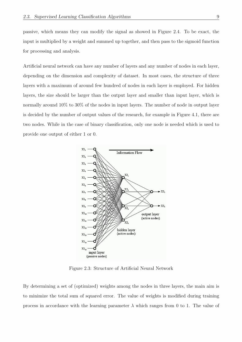
2.3. Supervised Learning Classification Algorithms 9
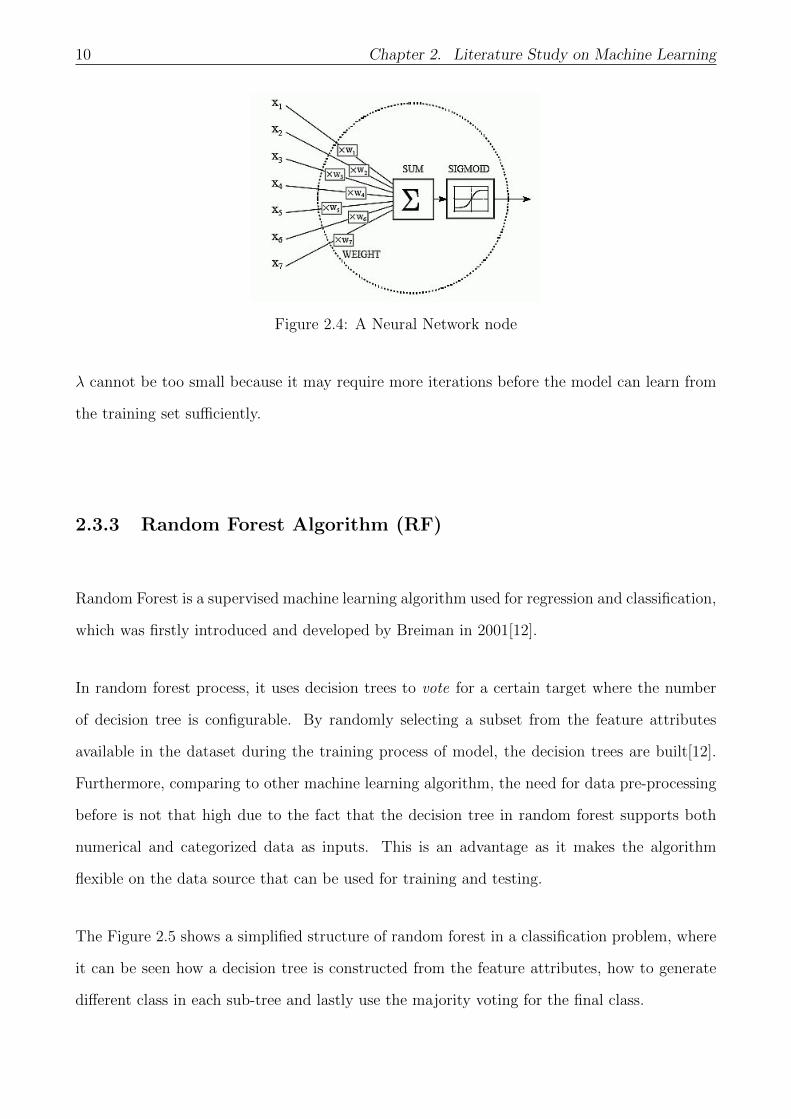
passive, which means they can modify the signal as showed in Figure 2.4. To be exact, the
input is multiplied by a weight and summed up together, and then pass to the sigmoid function
for processing and analysis.
Artificial neural network can have any number of layers and any number of nodes in each layer,
depending on the dimension and complexity of dataset. In most cases, the structure of three
layers with a maximum of around few hundred of nodes in each layer is employed. For hidden
layers, the size should be larger than the output layer and smaller than input layer, which is
normally around 10% to 30% of the nodes in input layers. The number of node in output layer
is decided by the number of output values of the research, for example in Figure 4.1, there are
two nodes. While in the case of binary classification, only one node is needed which is used to
provide one output of either 1 or 0.
Figure 2.3: Structure of Artificial Neural Network
By determining a set of (optimized) weights among the nodes in three layers, the main aim is
to minimize the total sum of squared error. The value of weights is modified during training
process in accordance with the learning parameter λ which ranges from 0 to 1. The value of
10 Chapter 2. Literature Study on Machine Learning
Figure 2.4: A Neural Network node
λ cannot be too small because it may require more iterations before the model can learn from
the training set sufficiently.
2.3.3 Random Forest Algorithm (RF)
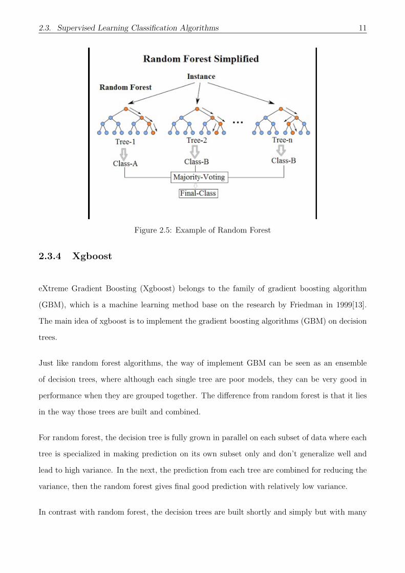
Random Forest is a supervised machine learning algorithm used for regression and classification,
which was firstly introduced and developed by Breiman in 2001[12].
In random forest process, it uses decision trees to vote for a certain target where the number
of decision tree is configurable. By randomly selecting a subset from the feature attributes
available in the dataset during the training process of model, the decision trees are built[12].
Furthermore, comparing to other machine learning algorithm, the need for data pre-processing
before is not that high due to the fact that the decision tree in random forest supports both
numerical and categorized data as inputs. This is an advantage as it makes the algorithm
flexible on the data source that can be used for training and testing.
The Figure 2.5 shows a simplified structure of random forest in a classification problem, where
it can be seen how a decision tree is constructed from the feature attributes, how to generate
different class in each sub-tree and lastly use the majority voting for the final class.
2.3. Supervised Learning Classification Algorithms 11
Figure 2.5: Example of Random Forest
2.3.4 Xgboost
eXtreme Gradient Boosting (Xgboost) belongs to the family of gradient boosting algorithm
(GBM), which is a machine learning method base on the research by Friedman in 1999[13].
The main idea of xgboost is to implement the gradient boosting algorithms (GBM) on decision
trees.
Just like random forest algorithms, the way of implement GBM can be seen as an ensemble
of decision trees, where although each single tree are poor models, they can be very good in
performance when they are grouped together. The difference from random forest is that it lies
in the way those trees are built and combined.
For random forest, the decision tree is fully grown in parallel on each subset of data where each
tree is specialized in making prediction on its own subset only and don’t generalize well and
lead to high variance. In the next, the prediction from each tree are combined for reducing the
variance, then the random forest gives final good prediction with relatively low variance.
In contrast with random forest, the decision trees are built shortly and simply but with many
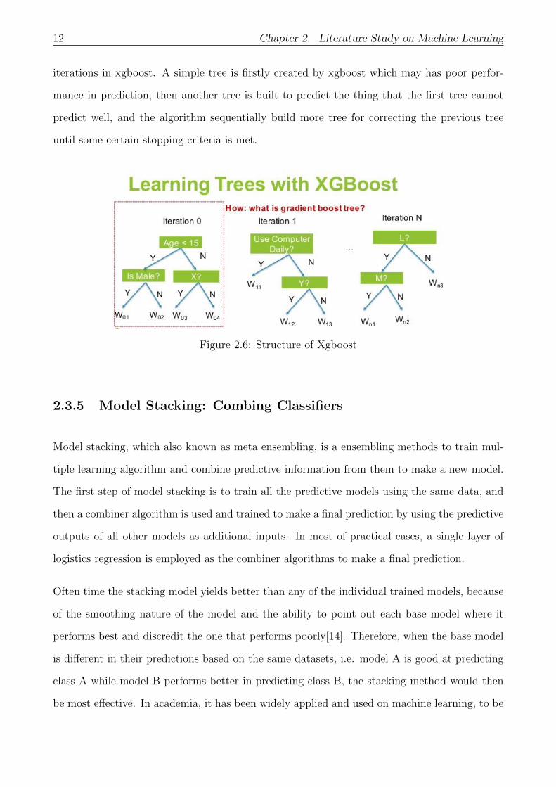
12 Chapter 2. Literature Study on Machine Learning
iterations in xgboost. A simple tree is firstly created by xgboost which may has poor perfor-
mance in prediction, then another tree is built to predict the thing that the first tree cannot
predict well, and the algorithm sequentially build more tree for correcting the previous tree
until some certain stopping criteria is met.
Figure 2.6: Structure of Xgboost
2.3.5 Model Stacking: Combing Classifiers
Model stacking, which also known as meta ensembling, is a ensembling methods to train mul-
tiple learning algorithm and combine predictive information from them to make a new model.
The first step of model stacking is to train all the predictive models using the same data, and
then a combiner algorithm is used and trained to make a final prediction by using the predictive
outputs of all other models as additional inputs. In most of practical cases, a single layer of
logistics regression is employed as the combiner algorithms to make a final prediction.
Often time the stacking model yields better than any of the individual trained models, because
of the smoothing nature of the model and the ability to point out each base model where it
performs best and discredit the one that performs poorly[14]. Therefore, when the base model
is different in their predictions based on the same datasets, i.e. model A is good at predicting
class A while model B performs better in predicting class B, the stacking method would then
be most effective. In academia, it has been widely applied and used on machine learning, to be
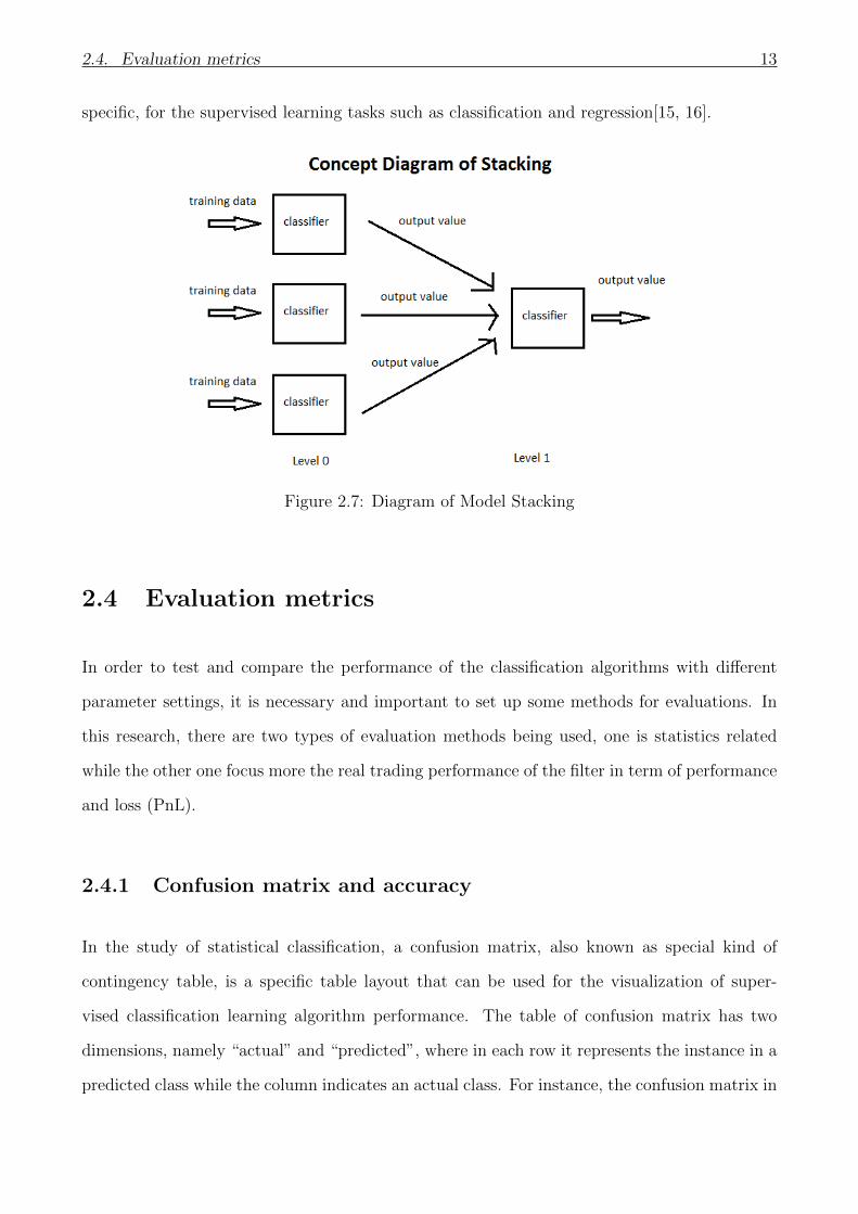
2.4. Evaluation metrics 13
specific, for the supervised learning tasks such as classification and regression[15, 16].
Figure 2.7: Diagram of Model Stacking
2.4 Evaluation metrics
In order to test and compare the performance of the classification algorithms with different
parameter settings, it is necessary and important to set up some methods for evaluations. In
this research, there are two types of evaluation methods being used, one is statistics related
while the other one focus more the real trading performance of the filter in term of performance
and loss (PnL).
2.4.1 Confusion matrix and accuracy
In the study of statistical classification, a confusion matrix, also known as special kind of
contingency table, is a specific table layout that can be used for the visualization of super-
vised classification learning algorithm performance. The table of confusion matrix has two
dimensions, namely “actual” and “predicted”, where in each row it represents the instance in a
predicted class while the column indicates an actual class. For instance, the confusion matrix in
14 Chapter 2. Literature Study on Machine Learning
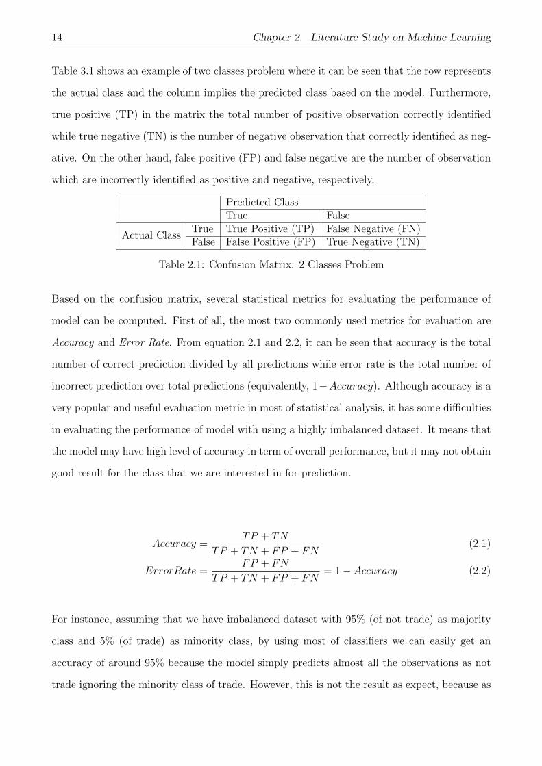
Table 3.1 shows an example of two classes problem where it can be seen that the row represents
the actual class and the column implies the predicted class based on the model. Furthermore,
true positive (TP) in the matrix the total number of positive observation correctly identified
while true negative (TN) is the number of negative observation that correctly identified as neg-
ative. On the other hand, false positive (FP) and false negative are the number of observation
which are incorrectly identified as positive and negative, respectively.
Predicted ClassTrue False
Actual ClassTrue True Positive (TP) False Negative (FN)False False Positive (FP) True Negative (TN)
Table 2.1: Confusion Matrix: 2 Classes Problem
Based on the confusion matrix, several statistical metrics for evaluating the performance of
model can be computed. First of all, the most two commonly used metrics for evaluation are
Accuracy and Error Rate. From equation 2.1 and 2.2, it can be seen that accuracy is the total
number of correct prediction divided by all predictions while error rate is the total number of
incorrect prediction over total predictions (equivalently, 1−Accuracy). Although accuracy is a
very popular and useful evaluation metric in most of statistical analysis, it has some difficulties
in evaluating the performance of model with using a highly imbalanced dataset. It means that
the model may have high level of accuracy in term of overall performance, but it may not obtain
good result for the class that we are interested in for prediction.
Accuracy =TP + TN
TP + TN + FP + FN(2.1)
ErrorRate =FP + FN
TP + TN + FP + FN= 1− Accuracy (2.2)
For instance, assuming that we have imbalanced dataset with 95% (of not trade) as majority
class and 5% (of trade) as minority class, by using most of classifiers we can easily get an
accuracy of around 95% because the model simply predicts almost all the observations as not
trade ignoring the minority class of trade. However, this is not the result as expect, because as

2.4. Evaluation metrics 15
a trading firm the main aim is to do as many trades as possible rather than doing nothing.
In order to measure the performance of model in dealing with the imbalanced dataset better,
another two types of metrics methods are used in this research. The first type is still statistics
related, which is the precision and recall, while the other one is the trading performance in
term of profit and loss (PnL) of the strategy with filter. A more detailed description regarding
these metrics will be given below.
2.4.2 Precision, Recall and F1-Score
In study of machine learning, it is known that precision and recall are both useful evaluation
metrics for measuring the performance of machine learning classifier, especially in processing
imbalanced dataset. Precision is the percentages of correct positive predictions over all positive
predictions (See Eq. 2.3), which is a measurement of how many positive predictions were true
positive observations. Recall is the fraction of all true positive prediction over all true positive
observations (See, Eq. 2.4), which is also known as True Positive Rate (TPR) or Sensitivity.
Recall gives a reflection of how good a model in predicting the positive case because it measures
how many actual positive observations are identified correctly. Similarly, there is also False
Positive Rate (FPR), which is proportion of all negative observation that are predicted wrongly
and gives an impression of how good a model in predicting the negative class (See, Eq. 2.5).
From the imbalanced example with 5% of trade observations as minority class (see Table 2.2),
both precision and recall reflect how good the model in identifying the minority class of trade,
so an ideal model for this case would have both high recall and high precision. In term of FPR,
the False Positive Rate should be as lower as possible since less wrong trades (False Positive)
are desired.
Lastly, with regards to the F1-Score, which is the harmonic mean of precision and recall in a
single measurement and ranges from 0 to 1. (See Eq. 2.6). It can be seen that the value of
F1-score is approximately the average of precision and recall when the two getting closed to
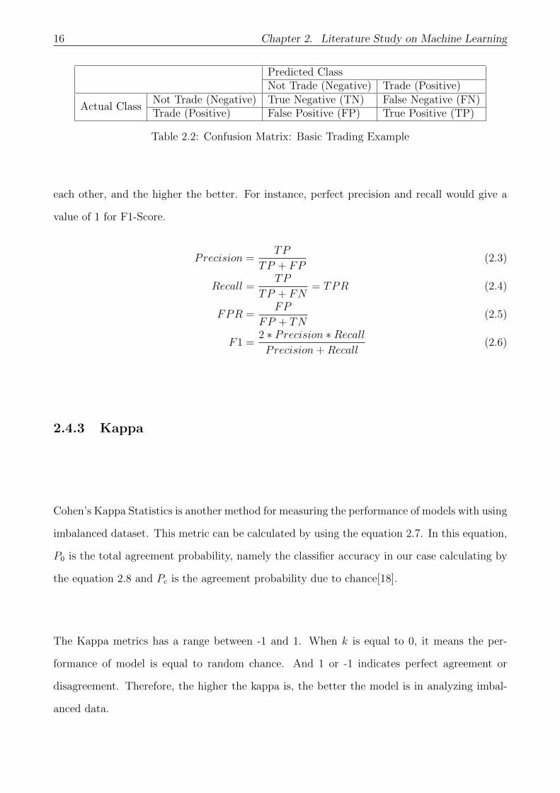
16 Chapter 2. Literature Study on Machine Learning
Predicted ClassNot Trade (Negative) Trade (Positive)
Actual ClassNot Trade (Negative) True Negative (TN) False Negative (FN)Trade (Positive) False Positive (FP) True Positive (TP)
Table 2.2: Confusion Matrix: Basic Trading Example
each other, and the higher the better. For instance, perfect precision and recall would give a
value of 1 for F1-Score.
Precision =TP
TP + FP(2.3)
Recall =TP
TP + FN= TPR (2.4)
FPR =FP
FP + TN(2.5)
F1 =2 ∗ Precision ∗RecallPrecision+Recall
(2.6)
2.4.3 Kappa
Cohen’s Kappa Statistics is another method for measuring the performance of models with using
imbalanced dataset. This metric can be calculated by using the equation 2.7. In this equation,
P0 is the total agreement probability, namely the classifier accuracy in our case calculating by
the equation 2.8 and Pc is the agreement probability due to chance[18].
The Kappa metrics has a range between -1 and 1. When k is equal to 0, it means the per-
formance of model is equal to random chance. And 1 or -1 indicates perfect agreement or
disagreement. Therefore, the higher the kappa is, the better the model is in analyzing imbal-
anced data.
2.4. Evaluation metrics 17
k =P0 − Pc
1− Pc
(2.7)
P0 =n∑
n=1
P (xnn) (2.8)
P1 =n∑
n=1
P (xn.)P (x.n) (2.9)
2.4.4 ROC and AUC
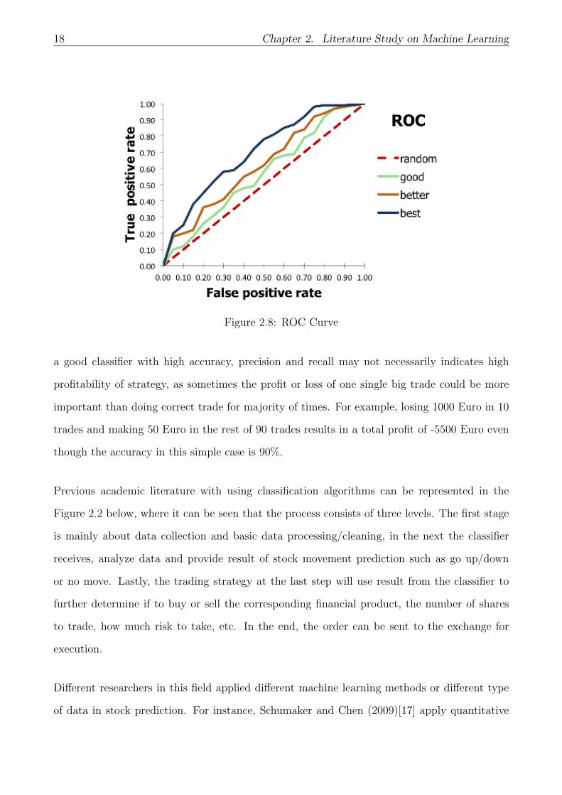
Receiver Operating Characteristic (ROC) curve is the third option for comparing the perfor-
mance of imbalanced data. The figure 2.2 below shows an example of ROC curve where the
x-axis is recall or false positive rate and the y-axis is the true positive rate.
As indicated in the plot, the best classifier is the one near the top left corner with small false
positive rate and large true positive rate. And the one on diagonal is purely random classifier.
The Area Under the ROC Curve (AUC) can be calculated by integrating the ROC curve, for
example, the top left one will have the largest AUC because the area under its curve is the
largest. And the random curve will have an area of 0.5. For those classifiers whose performance
is lower than the random one, their AUC will be lower than 0.5 as well. In most cases, AUC is
applied in binary classification problem for measuring the performance.
2.4.5 Performance of Profitability of the model
The reason for employing machine learning techniques in intraday trading is apparently simple
and direct, is to improve the overall profitability of trading strategies. Therefore, instead of
focusing on the statistical metric for evaluation, it is also necessary to check the effect of machine
learning application on the profitability of our algorithmic trading strategy, precisely to what
extent the filter of classifiers can improve the profitability.
Conducting the profitability analysis is necessary in this research, mainly due to the fact that
18 Chapter 2. Literature Study on Machine Learning
Figure 2.8: ROC Curve
a good classifier with high accuracy, precision and recall may not necessarily indicates high
profitability of strategy, as sometimes the profit or loss of one single big trade could be more
important than doing correct trade for majority of times. For example, losing 1000 Euro in 10
trades and making 50 Euro in the rest of 90 trades results in a total profit of -5500 Euro even
though the accuracy in this simple case is 90%.
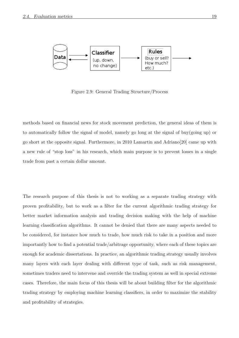
Previous academic literature with using classification algorithms can be represented in the
Figure 2.2 below, where it can be seen that the process consists of three levels. The first stage
is mainly about data collection and basic data processing/cleaning, in the next the classifier
receives, analyze data and provide result of stock movement prediction such as go up/down
or no move. Lastly, the trading strategy at the last step will use result from the classifier to
further determine if to buy or sell the corresponding financial product, the number of shares
to trade, how much risk to take, etc. In the end, the order can be sent to the exchange for
execution.
Different researchers in this field applied different machine learning methods or different type
of data in stock prediction. For instance, Schumaker and Chen (2009)[17] apply quantitative
2.4. Evaluation metrics 19
Figure 2.9: General Trading Structure/Process
methods based on financial news for stock movement prediction, the general ideas of them is
to automatically follow the signal of model, namely go long at the signal of buy(going up) or
go short at the opposite signal. Furthermore, in 2010 Lamartin and Adriano[20] came up with
a new rule of “stop loss” in his research, which main purpose is to prevent losses in a single
trade from past a certain dollar amount.
The research purpose of this thesis is not to working as a separate trading strategy with
proven profitability, but to work as a filter for the current algorithmic trading strategy for
better market information analysis and trading decision making with the help of machine
learning classification algorithms. It cannot be denied that there are many aspects needed to
be considered, for instance how much to trade, how much risk to take in a position and more
importantly how to find a potential trade/arbitrage opportunity, where each of these topics are
enough for academic dissertations. In practice, an algorithmic trading strategy usually involves
many layers with each layer dealing with different type of task, such as risk management,
sometimes traders need to intervene and override the trading system as well in special extreme
cases. Therefore, the main focus of this thesis will be about building filter for the algorithmic
trading strategy by employing machine learning classifiers, in order to maximize the stability
and profitability of strategies.

20 Chapter 2. Literature Study on Machine Learning
2.5 Model Validation
Model validation is a very important part of machine learning modelling. Once a model has
been trained and built on the training dataset and the corresponding model parameters have
been optimized, the next step is to evaluate the performance of model on an unseen subset
of dataset, namely the test set. It is not appropriate or even not right to use the training set
directly for performance evaluation because the model is biased toward the training set and
thus have a relatively good performance, such as high accuracy and precision. That’s why the
unseen subset (the test set) is applied for performance evaluation of trained model.
In the following subsections, two methods of model validation for measure the performance of
classifiers will be reviewed.
2.5.1 Holdout
The holdout method can be seen as the simplest method of model validation. In this method,
the dataset is randomly split into two sets, usually known as the training set and the test set,
respectively. The size of training set is arbitrary, but in most of cases the training set is larger
than the test set with the ratio ranging from 60%-40% to 90%-10% depending on the size of
whole dataset and the underlying problem. Firstly, the model is trained on the training set
only, and then the trained model is used to predict the target value using the data in the test
set. The main advantage of this simple method for cross validation is that it is efficient and
doesn’t take longer time to compute. However, there are also several problems associated with
this method, which is necessary to be considered.
First of all, as just mentioned the dataset is separated into two parts, this method obviously
reduces the amount of data available for training the model with many observations never being
used by the model. This problem can be mostly mitigated by applying random sub-sampling.
To be precise, the method is repeated for several times in this process with different subsets in
both the training set and the test set. For measuring the performance of model, the average of
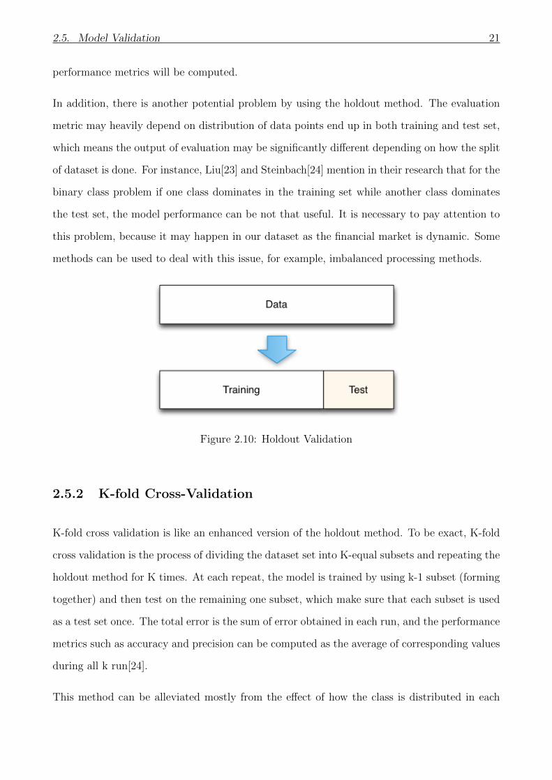
2.5. Model Validation 21
performance metrics will be computed.
In addition, there is another potential problem by using the holdout method. The evaluation
metric may heavily depend on distribution of data points end up in both training and test set,
which means the output of evaluation may be significantly different depending on how the split
of dataset is done. For instance, Liu[23] and Steinbach[24] mention in their research that for the
binary class problem if one class dominates in the training set while another class dominates
the test set, the model performance can be not that useful. It is necessary to pay attention to
this problem, because it may happen in our dataset as the financial market is dynamic. Some
methods can be used to deal with this issue, for example, imbalanced processing methods.
Figure 2.10: Holdout Validation
2.5.2 K-fold Cross-Validation
K-fold cross validation is like an enhanced version of the holdout method. To be exact, K-fold
cross validation is the process of dividing the dataset set into K-equal subsets and repeating the
holdout method for K times. At each repeat, the model is trained by using k-1 subset (forming
together) and then test on the remaining one subset, which make sure that each subset is used
as a test set once. The total error is the sum of error obtained in each run, and the performance
metrics such as accuracy and precision can be computed as the average of corresponding values
during all k run[24].
This method can be alleviated mostly from the effect of how the class is distributed in each
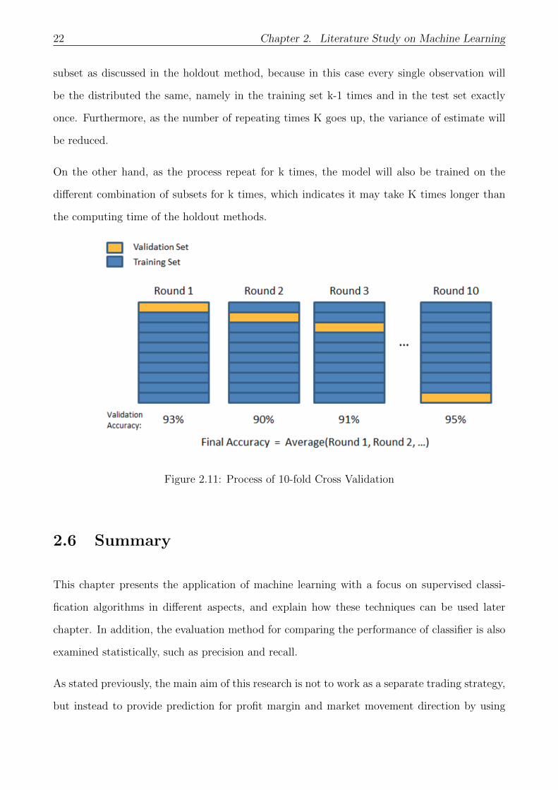
22 Chapter 2. Literature Study on Machine Learning
subset as discussed in the holdout method, because in this case every single observation will
be the distributed the same, namely in the training set k-1 times and in the test set exactly
once. Furthermore, as the number of repeating times K goes up, the variance of estimate will
be reduced.
On the other hand, as the process repeat for k times, the model will also be trained on the
different combination of subsets for k times, which indicates it may take K times longer than
the computing time of the holdout methods.
Figure 2.11: Process of 10-fold Cross Validation
2.6 Summary
This chapter presents the application of machine learning with a focus on supervised classi-
fication algorithms in different aspects, and explain how these techniques can be used later
chapter. In addition, the evaluation method for comparing the performance of classifier is also
examined statistically, such as precision and recall.
As stated previously, the main aim of this research is not to work as a separate trading strategy,
but instead to provide prediction for profit margin and market movement direction by using
2.6. Summary 23
machine learning algorithms, which can improve the ability of trading strategy of better market
information processing and trading decision making. As a result, the effect of classifiers (working
as filter) on the profitability of trading strategy will also be compared in term of Profit and
Loss (PnL).
Lastly, this chapter presents two approaches for model validation, namely the holdout meth-
ods and the k-fold cross validation by giving the description about how it works and their
corresponding advantages and disadvantages in model testing.

Chapter 3
Project Design and Data Engineering
3.1 Project Description
As mentioned previously, the main purpose of this project is to create an in-built filter inside
our trading system based on machine learning classifiers to enhance the overall profitability
of the algorithmic trading strategies that currently operating in ATG, in term of improving
intraday market information analysis and systematic trading decision making.
The architecture of this in-built filter plays a very important role in the system. Since the need
from trading strategies are different, the filter is therefore separated into two layers in order to
better meet the requirement from strategies and improve the efficiency of whole trading system,
where some of strategies use both two layers and some use the first layer only. However, for
the academic purpose, this paper focus on the two-layer architecture and thus use the strategy
in the need of two layers for testing and performance comparison. More details regarding the
architecture will be given in the following section 3.2.
With regards to the trading dataset, it is originally from the Japanese Exchange Market-Nikkei
with duration of 1 year from 11/2015 to 11/2016. The dataset has two types of data group
with in total of 1852154 observations where each observation is a single trade. The first group
of data contains around 20 intraday market features that can be used for classification of each
24

3.2. Architecture of the Filter 25
instance (trade), such as moving average in recent short period. In another group, there are
several trade execution related variables, like trade price and trading quantity, which is mainly
used to calculate the corresponding profit and loss (PnL) of one trade, and further determine
and compute the target variable for this research. However, for confidential reasons, it’s not
possible and not allowed to provide any information including definition regarding some of the
market features that used in this research project. In the section 3.3, more details about the
dataset and further data engineering will presented.
Lastly, in the section 3.4, there is a short discussion regarding the trade-off between performance
(i.e. accuracy) and efficiency (time/speed) of the algorithm[25], especially in the case of trading.
Typically, the more complicated the model is, the more time it takes to compute results, the
better results it can achieve. But in high or medium frequency trading (HFT), speed does play
a very important role which the less time the system spends on making decision, the higher
possibility for the strategy to seize the opportunity. If it takes too long, it will miss the chance
although the prediction or decision is correct. Hence, it is very importance to find a balance
between performance and efficiency.
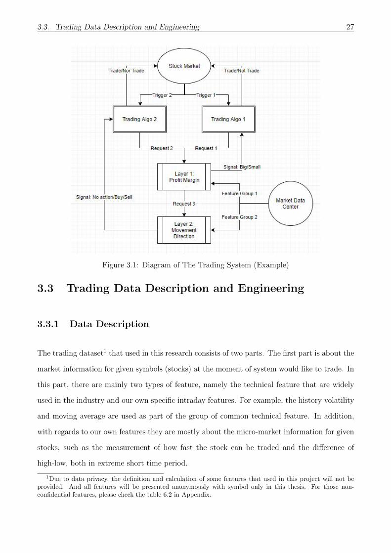
3.2 Architecture of the Filter
The filter consists of two layers, where both two layers can work either separately or together,
depending on the need of different automated trading strategies. The basic structure of trading
system with the filter and trading strategies can be seen in the picture below (Figure 3.1),
which illustrates how the whole system works.
To be precise, there are two trading algorithms in the system with different needs from the
filter system. For example, when something happens in the market and triggers the trading
algorithm 1 to do a trade, then this algorithm immediately sends the request 1 to the first layer
to ask for prediction regarding the profit margin of this potential trade based on current market
situation. After getting data from the data center and doing corresponding analysis, the layer

26 Chapter 3. Project Design and Data Engineering
1 generates a signal about the potential size, then send back the signal to the trading algorithm
1, and lastly the trading algorithm 2 will therefore determine whether trade or not at this
potential moment based on the signal. If the signal shows a big profit margin, the trading algo
1 will thus participate in this trade. In fact, the majority of trading algorithms that currently
running in the system only require information from the first layer, for the purpose of excluding
small trade with low level of potential profit margin.
However, the work structure is bit different for trading algorithms 2 because it requests more
information from the filter including both the profit margin and direction of market movement.
In this case, the layer 2 is employed to make forecast about market movement. To be specific,
as we can see in the plot, the layer 1 send a new request to the second layer with information
about the profit margin, then the layer 2 use the information from both the first layer and
the market data center to make corresponding prediction about movement direction. After
analysis is done, it sends back the signal, namely no action/buy/sell, to the trading algorithm
2. Again, based on the outcome of signal the trading algo 2 will determine if to do a trade
or not, and the direction of trade, short or long. For instance, if at the first layer the profit
margin is predicted as small, the layer 2 will directly send a signal of no action to the trading
algo 2 and thus no order will be sent out. On the other hand, if the profit margin is identified
as big, the layer 2 starts analysis and makes prediction regarding movement direction based on
the market situation. If the market is predicted as going down, the layer 2 sends out a signal
of sell to the trading algo 2, and as a result the algo 2 will send a buy order to the market.
As said previously, this diagram of trading system is not the full version because it doesn’t
include other parts, such as the risk management and post trade analysis. That is to say,
this filter with two layers is more or less working as an advisor for the trading algorithm,
which provides suggestions about the potential trade based on market information and gives
corresponding signal to the algorithms. Again, for the purpose of testing the performance of
two layers, a trading strategy similar to the trading algorithm 1 in the diagram is used in
following research.
3.3. Trading Data Description and Engineering 27
Figure 3.1: Diagram of The Trading System (Example)
3.3 Trading Data Description and Engineering
3.3.1 Data Description
The trading dataset1 that used in this research consists of two parts. The first part is about the
market information for given symbols (stocks) at the moment of system would like to trade. In
this part, there are mainly two types of feature, namely the technical feature that are widely
used in the industry and our own specific intraday features. For example, the history volatility
and moving average are used as part of the group of common technical feature. In addition,
with regards to our own features they are mostly about the micro-market information for given
stocks, such as the measurement of how fast the stock can be traded and the difference of
high-low, both in extreme short time period.
1Due to data privacy, the definition and calculation of some features that used in this project will not beprovided. And all features will be presented anonymously with symbol only in this thesis. For those non-confidential features, please check the table 6.2 in Appendix.
28 Chapter 3. Project Design and Data Engineering
The second part is trade execution data such as trading price including buy and sell price,
trading quantity and holding time, which is the output from the backtesting of trading strategy
that used for checking and comparing the performance of machine learning classifiers.
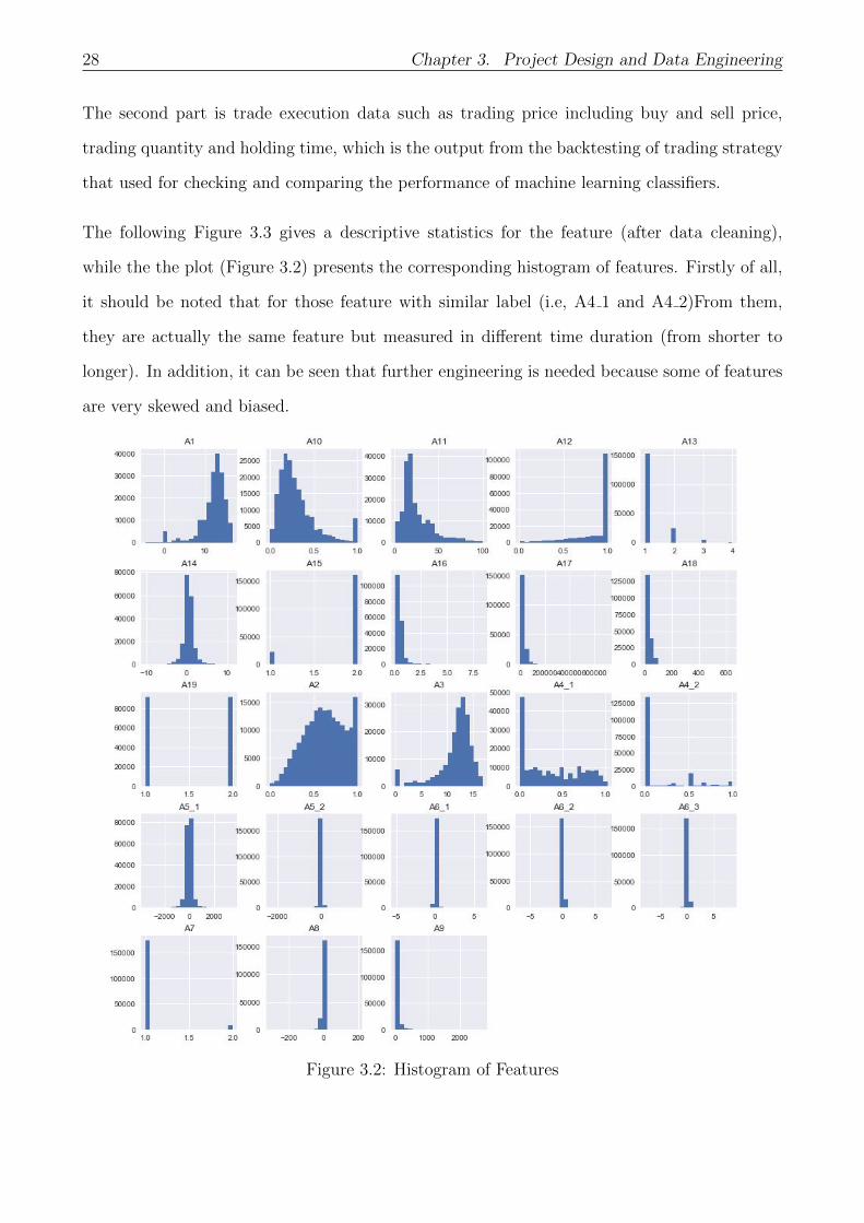
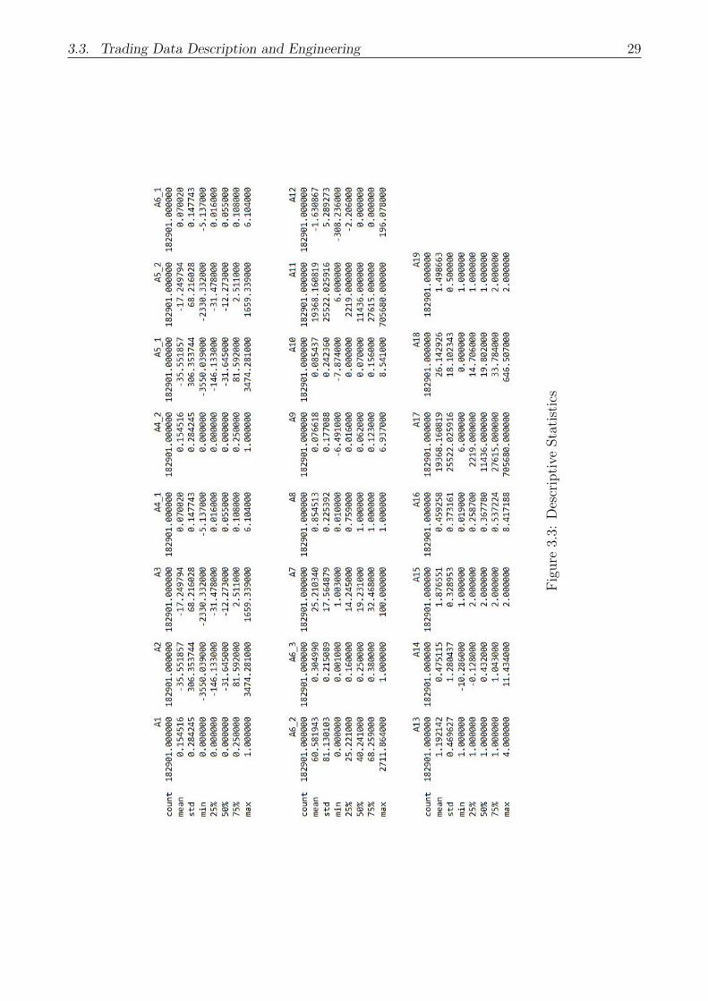
The following Figure 3.3 gives a descriptive statistics for the feature (after data cleaning),
while the the plot (Figure 3.2) presents the corresponding histogram of features. Firstly of all,
it should be noted that for those feature with similar label (i.e, A4 1 and A4 2)From them,
they are actually the same feature but measured in different time duration (from shorter to
longer). In addition, it can be seen that further engineering is needed because some of features
are very skewed and biased.
Figure 3.2: Histogram of Features
3.3. Trading Data Description and Engineering 29
Fig
ure
3.3:
Des
crip
tive
Sta
tist
ics
30 Chapter 3. Project Design and Data Engineering
3.3.2 Data Pre-Processing
Data pre-processing is a very important process before modelling, because it prepares the
data, make it ready for use in a machine learning model and thus make the model more
robust. Although recent development in technology has made the trading data more reliable
comparing to the past, pre-processing is still a necessary step before doing further statistical
analysis because it can guarantee the integrity of the machine learning model built. In general,
data-reprocessing has two main tasks, namely data cleaning and data transformation[27].
After data cleaning by removing invalid observations(values), the total number of observation in
the dataset decreases from 1852154 to 182901 as showed in the descriptive picture above. Then
the next step is data transformation, as it can be found that some of features have different
and relatively large scale.
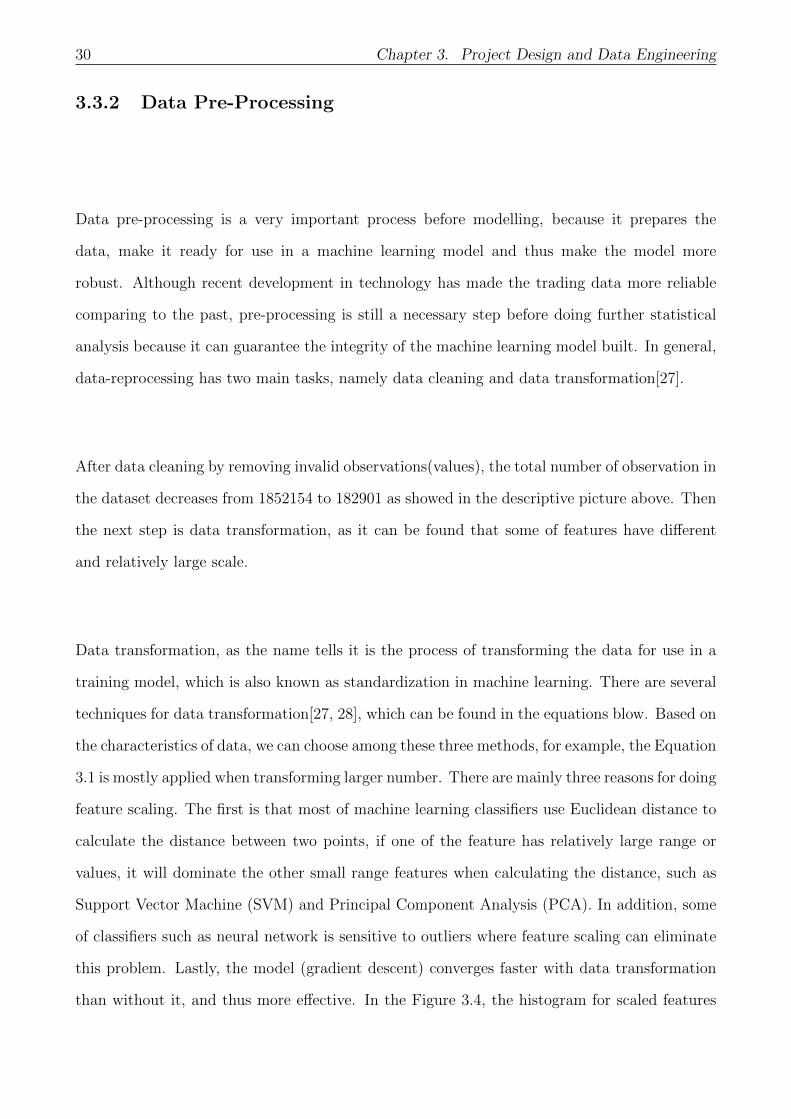
Data transformation, as the name tells it is the process of transforming the data for use in a
training model, which is also known as standardization in machine learning. There are several
techniques for data transformation[27, 28], which can be found in the equations blow. Based on
the characteristics of data, we can choose among these three methods, for example, the Equation
3.1 is mostly applied when transforming larger number. There are mainly three reasons for doing
feature scaling. The first is that most of machine learning classifiers use Euclidean distance to
calculate the distance between two points, if one of the feature has relatively large range or
values, it will dominate the other small range features when calculating the distance, such as
Support Vector Machine (SVM) and Principal Component Analysis (PCA). In addition, some
of classifiers such as neural network is sensitive to outliers where feature scaling can eliminate
this problem. Lastly, the model (gradient descent) converges faster with data transformation
than without it, and thus more effective. In the Figure 3.4, the histogram for scaled features
3.3. Trading Data Description and Engineering 31
can be found.
xscaled =x− µσ
(3.1)
xscaled = log(x) (3.2)
xscaled =x− xmin
xmax − xmin
(3.3)
Figure 3.4: Histogram of Scaled Features
32 Chapter 3. Project Design and Data Engineering
3.3.3 Feature Engineering
Target Variable
As stated previously in chapter 2, the supervised learning algorithm is used in this research
which indicates it is a must to define the target variable. The purpose of two layers in the filter
system is different where the first layer is used to forecast the profit margin of potential trade
in short term while the second layer is to determine the direction of short-term movement of
stock. Hence, we can define the target variable for two layers as follows.
When talking about the stock movement, traders are most interested in the big movement be-
cause big movements can possibly lead to high profit margin while small movements sometimes
cannot even cover the cost, i.e. transaction costs. Therefore, what the first layer is a binary
classifier, to predict the profit margin (size) of a potential trade that the strategy wants to do.
For the computation and measurement of the size, the basis point (BPS) is employed and 1
BPS is equal to 0.01%. The stock price difference in short time term is used and computed
to get percentage change in BPS. According to characteristics of the testing strategy and the
market rule of Nikkei, 30 BPS is defined as the threshold which means for those trades with
more than 30 BPS potential profit margin they are regarded as big trades, labeled as 1. And
for those small trades with profit margin smaller than 30 BPS, it is labeled as 0. Lastly, from
the backtesting results there is one interesting fact that around 80% percent of total profits
come from these big trades we selected, which accounts for 25% of the total number of trades.
This finding is sort of consistent with the famous Pareto principle (also known as 80/20 rule),
which states that for many events, roughly 80% of the effects come from 20% of the causes.
As to the direction of movement, it is then relatively easier. If the price goes down in short
time term we then define it as go short because this is the way to make profit. If it goes up,
then direction is go long. However, there is one need to be added, as we are only interested in
the big movements, so for those small trades that defined in the first layer, no action is taken.
Therefore, there are three classes for the target variable direction, namely go long (1), go short
3.3. Trading Data Description and Engineering 33
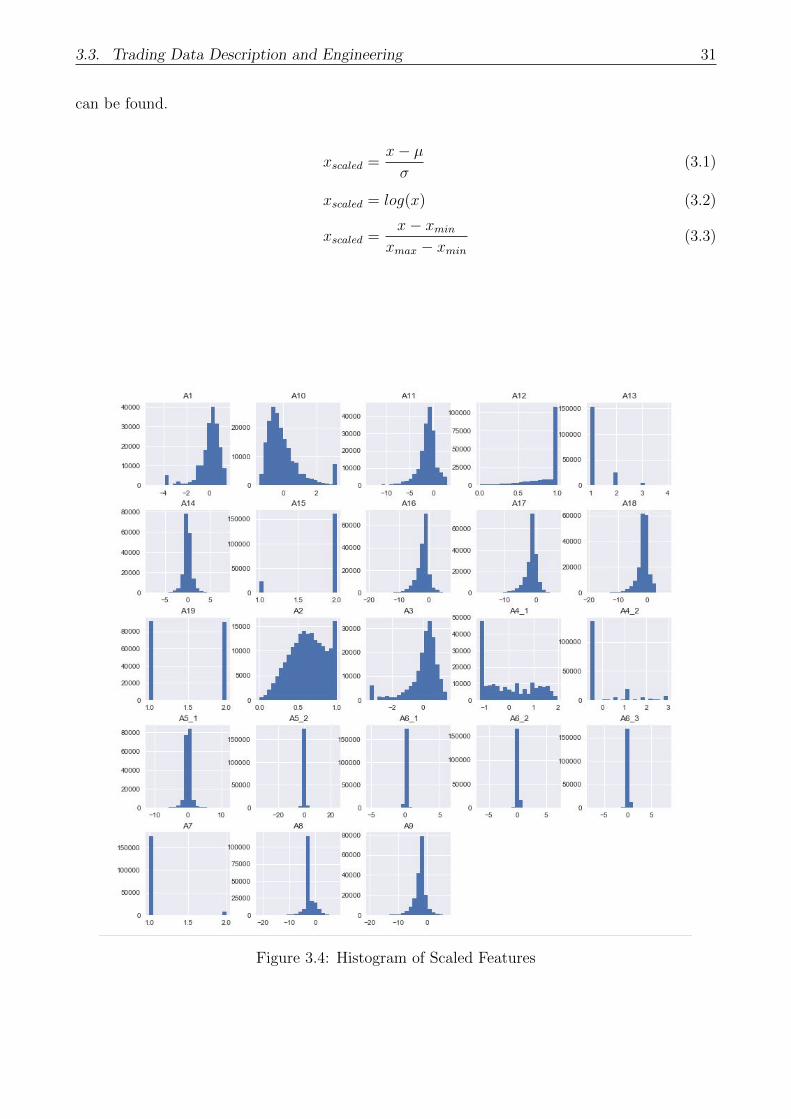
(2) and no action (0).
Figure 3.5: Histogram of Target Variables
New Attribute
Anything that happens in the market can possibly lead to a change in the stock price, so is
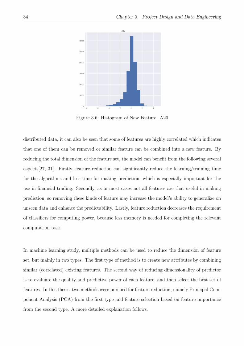
our trade. Therefore, a new feature (A20) is created and added to the input feature set which
measures the relative size of our potential order comparing to open orders in the order book.
For the corresponding histogram, please see Figure 3.6.
3.3.4 Feature Reduction
In this research, there are in total 24 features, but distributed in two groups with one features
in common. The group 1 is used for the first layer with in total of 19 features, while group 2
for the second layer has 6 features only. Therefore, for the first layer there is a potential need
for feature reduction. Since each feature adds another one more dimension to the search space
for the model, the higher the dimension the harder the problem to solve. In addition, from
the correlation plot based on the Spearman Rank Test[30] which is applied on non-normally
34 Chapter 3. Project Design and Data Engineering
Figure 3.6: Histogram of New Feature: A20
distributed data, it can also be seen that some of features are highly correlated which indicates
that one of them can be removed or similar feature can be combined into a new feature. By
reducing the total dimension of the feature set, the model can benefit from the following several
aspects[27, 31]. Firstly, feature reduction can significantly reduce the learning/training time
for the algorithms and less time for making prediction, which is especially important for the
use in financial trading. Secondly, as in most cases not all features are that useful in making
prediction, so removing these kinds of feature may increase the model’s ability to generalize on
unseen data and enhance the predictability. Lastly, feature reduction decreases the requirement
of classifiers for computing power, because less memory is needed for completing the relevant
computation task.
In machine learning study, multiple methods can be used to reduce the dimension of feature
set, but mainly in two types. The first type of method is to create new attributes by combining
similar (correlated) existing features. The second way of reducing dimensionality of predictor
is to evaluate the quality and predictive power of each feature, and then select the best set of
features. In this thesis, two methods were pursued for feature reduction, namely Principal Com-
ponent Analysis (PCA) from the first type and feature selection based on feature importance
from the second type. A more detailed explanation follows.
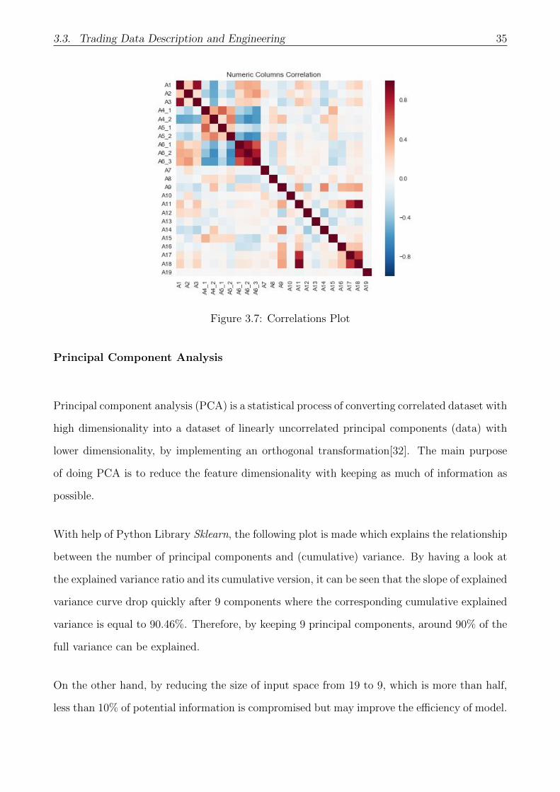
3.3. Trading Data Description and Engineering 35
Figure 3.7: Correlations Plot
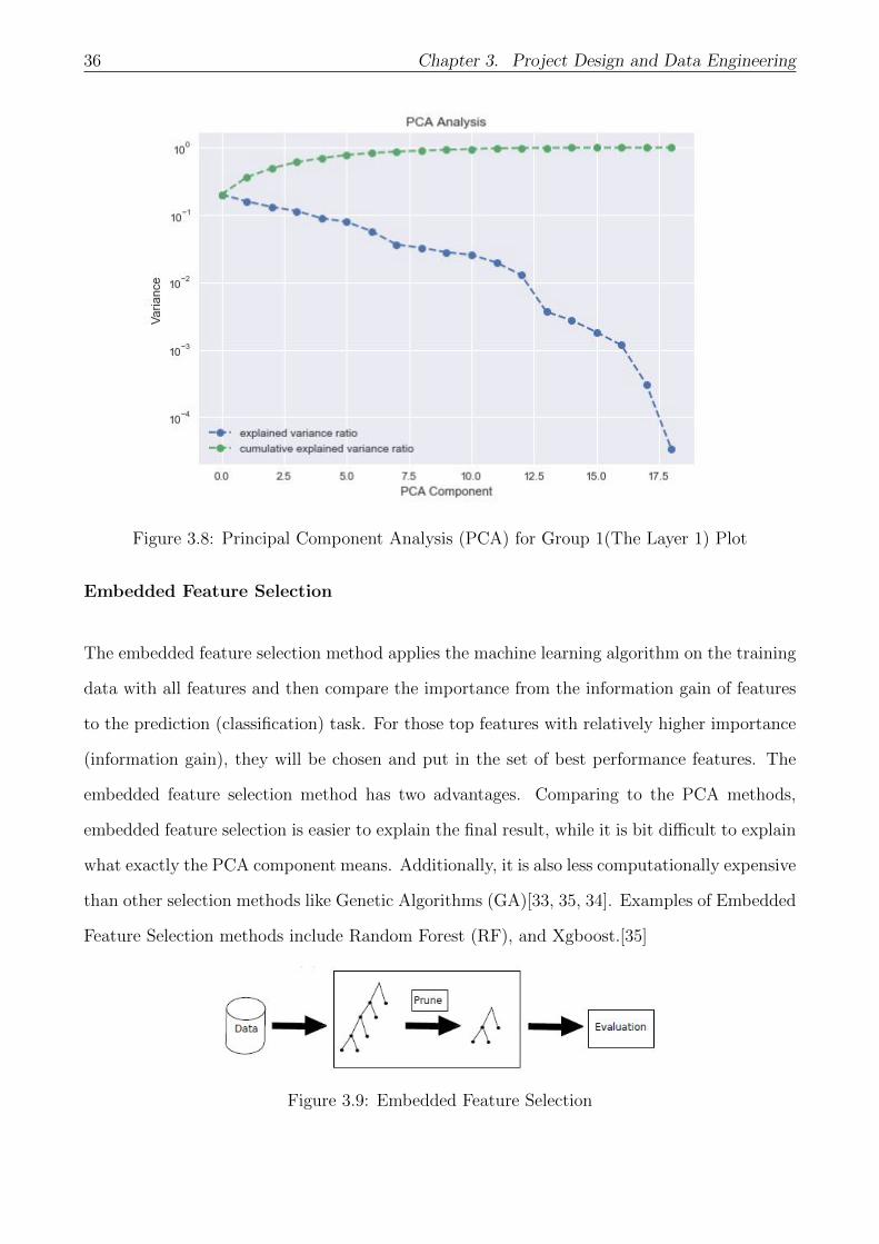
Principal Component Analysis
Principal component analysis (PCA) is a statistical process of converting correlated dataset with
high dimensionality into a dataset of linearly uncorrelated principal components (data) with
lower dimensionality, by implementing an orthogonal transformation[32]. The main purpose
of doing PCA is to reduce the feature dimensionality with keeping as much of information as
possible.
With help of Python Library Sklearn, the following plot is made which explains the relationship
between the number of principal components and (cumulative) variance. By having a look at
the explained variance ratio and its cumulative version, it can be seen that the slope of explained
variance curve drop quickly after 9 components where the corresponding cumulative explained
variance is equal to 90.46%. Therefore, by keeping 9 principal components, around 90% of the
full variance can be explained.
On the other hand, by reducing the size of input space from 19 to 9, which is more than half,
less than 10% of potential information is compromised but may improve the efficiency of model.
36 Chapter 3. Project Design and Data Engineering
Figure 3.8: Principal Component Analysis (PCA) for Group 1(The Layer 1) Plot
Embedded Feature Selection
The embedded feature selection method applies the machine learning algorithm on the training
data with all features and then compare the importance from the information gain of features
to the prediction (classification) task. For those top features with relatively higher importance
(information gain), they will be chosen and put in the set of best performance features. The
embedded feature selection method has two advantages. Comparing to the PCA methods,
embedded feature selection is easier to explain the final result, while it is bit difficult to explain
what exactly the PCA component means. Additionally, it is also less computationally expensive
than other selection methods like Genetic Algorithms (GA)[33, 35, 34]. Examples of Embedded
Feature Selection methods include Random Forest (RF), and Xgboost.[35]
Figure 3.9: Embedded Feature Selection

3.3. Trading Data Description and Engineering 37
3.3.5 Imbalanced Data and Solutions
As can be seen in the Figure 3.5, it is normal to have the class imbalance problem in trading
datasets with more observations of a certain class than the others, i.e. much more small trades
than big trades in term of the profit margin. In general, a machine learning classifier may
have a bias with regards to the majority class and thus identify the minority class wrongly by
training the classifier on imbalanced datasets. This is mainly because identifying the majority
class is in favor of improving accuracy, thus the classifier misclassifies the minority class as
the majority class more often[36]. In the case of dealing with highly imbalanced dataset (i.e
99% majority/ 1% minority), the classifier may obtain a very high accuracy by ignoring and
misclassifying the minority class. This would be a problem for the research if the minority class
is of particular interest.
As to stock trading, traders/trading algorithms are interested in the large movements with
high level of profit margin in which the big movements are mostly the minority class. In order
to improve the performance of identifying the minority class of big trades, certain procedures
need to be taken to deal with imbalanced problem in the training dataset. There are two
types of approaches that can be applied to overcome the issue of imbalance problem, namely
undersampling and oversampling, depending on the size of training set.
To be precise, when the size of dataset is not big, or the number of observation is not that
sufficient, the oversampling method is used to increase the observation of minority class by
using techniques such as random oversampling and Synthetic Minority Oversampling Technique
(SMOTE)[37]. On the contrary, undersampling method balance the ratio between the majority
class and the minority class in the dataset by removing the instance of the abundant class, which
is especially useful when quantity of data is sufficient. There are several techniques in removing
the sample in majority class, for example, Edited Nearest Neighbours Rule[38], neighbourhood
cleaning rule[39], one-sided selection method[40] and removing Tomeks links[41]. In addition,
there is also a hybrid approach that combines oversampling and undersampling together. For
instance, the SMOTEENN method is to perform oversampling using SMOTE and follow by
38 Chapter 3. Project Design and Data Engineering
under-sampling using the Edited Nearest Neighbours[42]. In both two approaches mentioned
above, by either removing the observation in the majority class or increasing the instance of
minority class, a new balanced dataset can be obtained for further training and modelling.
However, in this project, there is a preference for undersampling method over the oversampling
for several reasons. Firstly, the undersampling method is in favor because the size of training
set is sufficiently large for training the model. Secondly, since there is high requirement for
the efficiency of classifiers which will be discussed in the next session, the undersampling is
preferred since it reduces the size of training set by removing the abundant instance in the
majority class and thus saves training time.
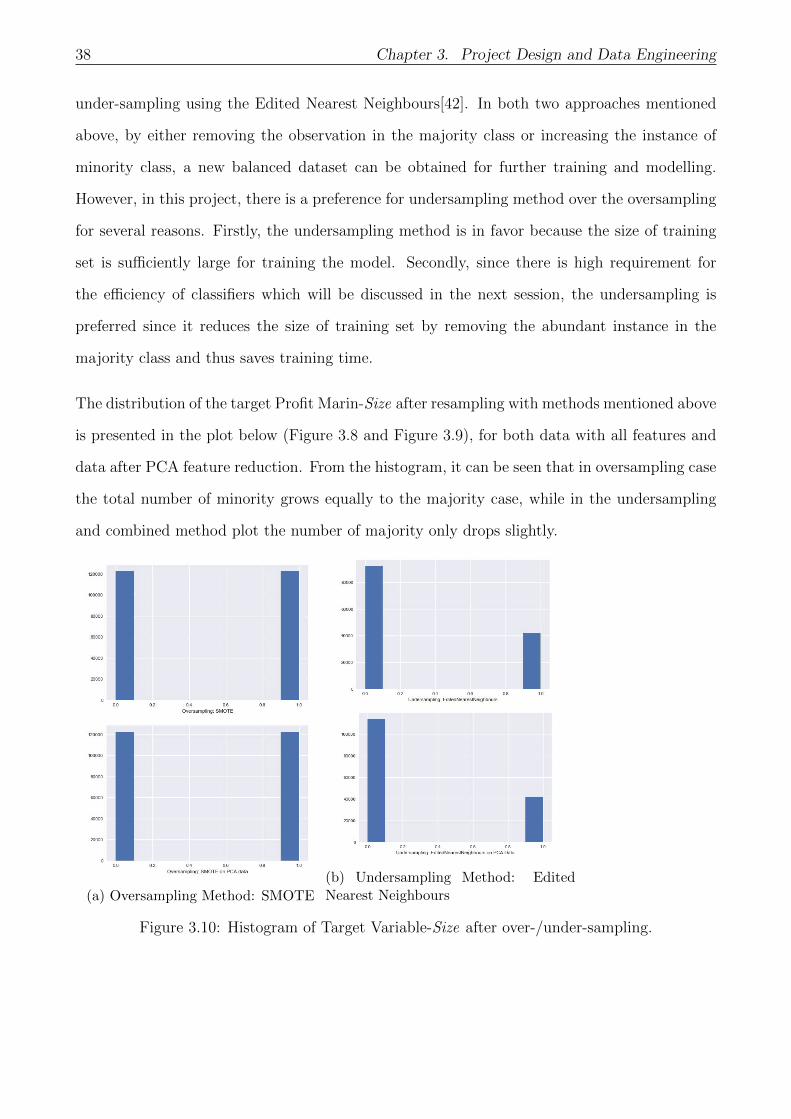
The distribution of the target Profit Marin-Size after resampling with methods mentioned above
is presented in the plot below (Figure 3.8 and Figure 3.9), for both data with all features and
data after PCA feature reduction. From the histogram, it can be seen that in oversampling case
the total number of minority grows equally to the majority case, while in the undersampling
and combined method plot the number of majority only drops slightly.
(a) Oversampling Method: SMOTE
(b) Undersampling Method: EditedNearest Neighbours
Figure 3.10: Histogram of Target Variable-Size after over-/under-sampling.
3.4. Performance and Efficiency 39
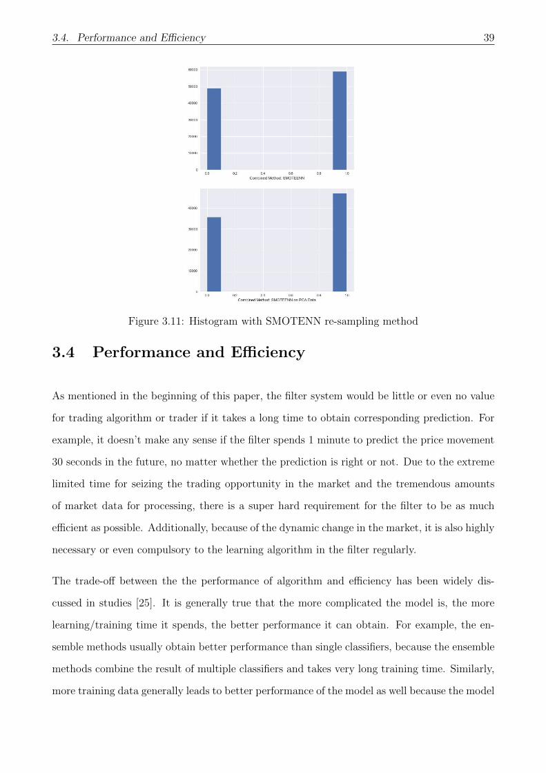
Figure 3.11: Histogram with SMOTENN re-sampling method
3.4 Performance and Efficiency
As mentioned in the beginning of this paper, the filter system would be little or even no value
for trading algorithm or trader if it takes a long time to obtain corresponding prediction. For
example, it doesn’t make any sense if the filter spends 1 minute to predict the price movement
30 seconds in the future, no matter whether the prediction is right or not. Due to the extreme
limited time for seizing the trading opportunity in the market and the tremendous amounts
of market data for processing, there is a super hard requirement for the filter to be as much
efficient as possible. Additionally, because of the dynamic change in the market, it is also highly
necessary or even compulsory to the learning algorithm in the filter regularly.
The trade-off between the the performance of algorithm and efficiency has been widely dis-
cussed in studies [25]. It is generally true that the more complicated the model is, the more
learning/training time it spends, the better performance it can obtain. For example, the en-
semble methods usually obtain better performance than single classifiers, because the ensemble
methods combine the result of multiple classifiers and takes very long training time. Similarly,
more training data generally leads to better performance of the model as well because the model

40 Chapter 3. Project Design and Data Engineering
have more data to learn the pattern or relationship inside the dataset. However, there is also a
point such that more data (those old data) cannot lead to a better performance of the model,
especially in the study of finance[43], because the predictability in the financial market may
disappear, and the market may constantly evolve.
Increasing the complexity of models does not necessarily improve performance, but on the other
hand negatively affect the efficiency of model. As a result, for this research, the most important
thing is to find a balance point between model efficiency and model performance, instead of
pursuing extreme high performance of the model.

Chapter 4
Experiments and Outputs
The chapter 2 gives a framework of how the machine learning techniques can be applied in
financial prediction (classification) problem, which mainly includes descriptions of different
classification algorithms in machine learning, performance evaluation by using statistical per-
formance metrics and profitability analysis, and lastly model validation/testing with help of the
holdout method and k-fold cross-validation. The first part chapter 3 presents an introduction
to the framework of filters and their connections with trading algorithms and other parts in the
trading system. The rest of chapter 3 mainly focuses on the data engineering process which
should be done before training the model including data cleaning and standardization, feature
engineering such as defining and calculating the target variable and creating new attributes,
feature reduction by using principal component analysis(PCA) & embedded feature selection
method and the imbalanced data processing.
In this chapter, the purpose is to present the experiment performance of the classification
filter on the test dataset with respect to different algorithms and different data engineering
methodologies. To make it clearer to understand the whole architecture of the filter system,
the outputs is presented in the following order. In the beginning, results correspond to the first
layer with purpose of identifying the size of potential profit margin will be given. Secondly, the
test performance of the layer-2 for predicting the direction of market movement will be showed.
41
42 Chapter 4. Experiments and Outputs
Lastly, as the main idea of this project is to connect two layers together to improve the overall
profitability of trading strategy, the experiment outcomes of combined system are of interest,
in term of statistical performance and the profitability.
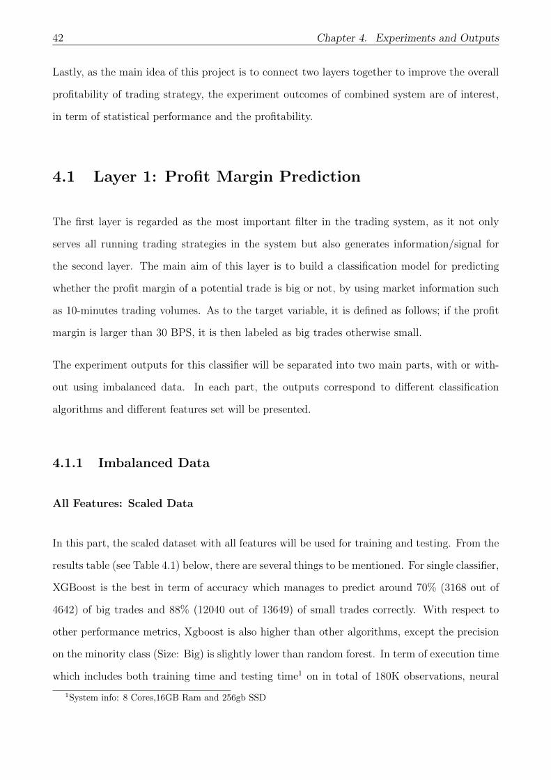
4.1 Layer 1: Profit Margin Prediction
The first layer is regarded as the most important filter in the trading system, as it not only
serves all running trading strategies in the system but also generates information/signal for
the second layer. The main aim of this layer is to build a classification model for predicting
whether the profit margin of a potential trade is big or not, by using market information such
as 10-minutes trading volumes. As to the target variable, it is defined as follows; if the profit
margin is larger than 30 BPS, it is then labeled as big trades otherwise small.
The experiment outputs for this classifier will be separated into two main parts, with or with-
out using imbalanced data. In each part, the outputs correspond to different classification
algorithms and different features set will be presented.
4.1.1 Imbalanced Data
All Features: Scaled Data
In this part, the scaled dataset with all features will be used for training and testing. From the
results table (see Table 4.1) below, there are several things to be mentioned. For single classifier,
XGBoost is the best in term of accuracy which manages to predict around 70% (3168 out of
4642) of big trades and 88% (12040 out of 13649) of small trades correctly. With respect to
other performance metrics, Xgboost is also higher than other algorithms, except the precision
on the minority class (Size: Big) is slightly lower than random forest. In term of execution time
which includes both training time and testing time1 on in total of 180K observations, neural
1System info: 8 Cores,16GB Ram and 256gb SSD
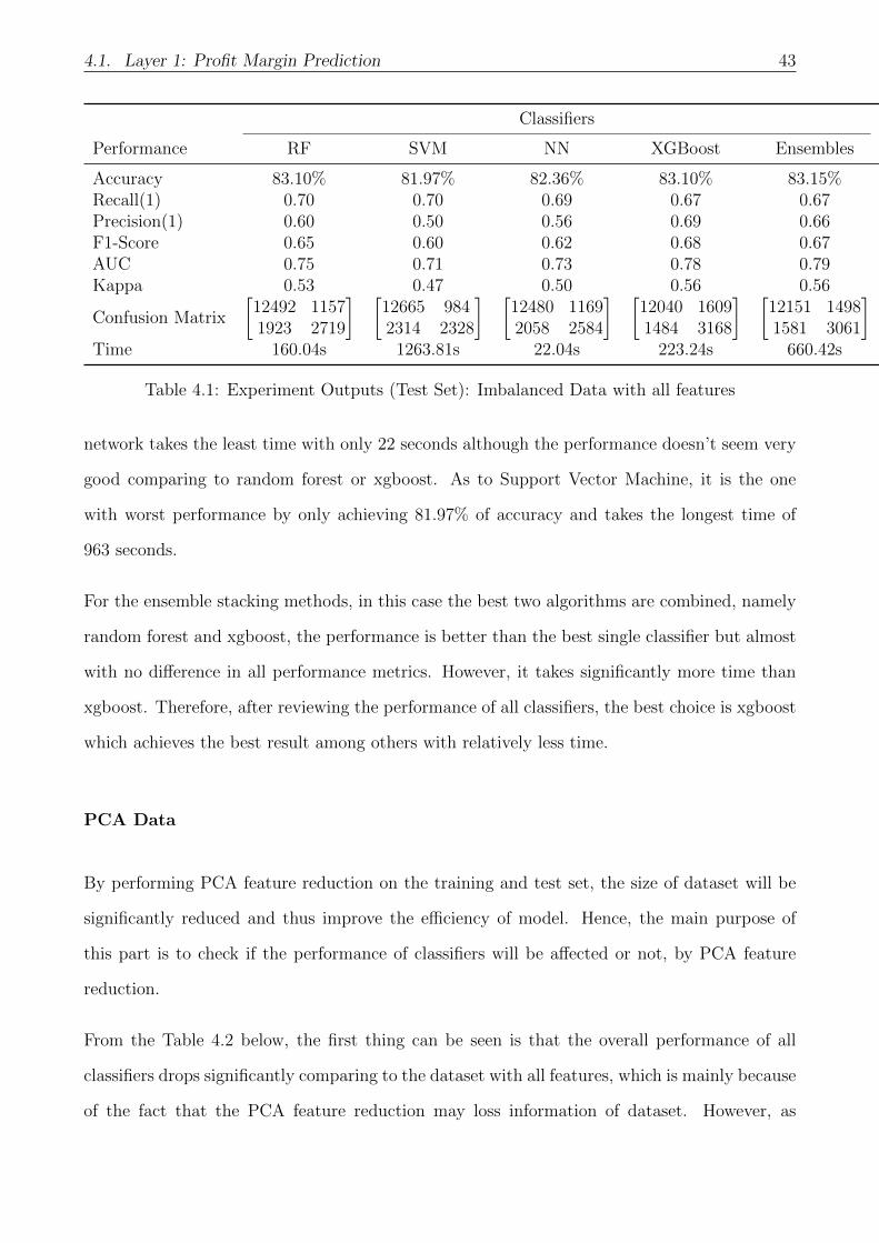
4.1. Layer 1: Profit Margin Prediction 43
Classifiers
Performance RF SVM NN XGBoost Ensembles
Accuracy 83.10% 81.97% 82.36% 83.10% 83.15%Recall(1) 0.70 0.70 0.69 0.67 0.67Precision(1) 0.60 0.50 0.56 0.69 0.66F1-Score 0.65 0.60 0.62 0.68 0.67AUC 0.75 0.71 0.73 0.78 0.79Kappa 0.53 0.47 0.50 0.56 0.56
Confusion Matrix
[12492 11571923 2719
] [12665 9842314 2328
] [12480 11692058 2584
] [12040 16091484 3168
] [12151 14981581 3061
]Time 160.04s 1263.81s 22.04s 223.24s 660.42s
Table 4.1: Experiment Outputs (Test Set): Imbalanced Data with all features
network takes the least time with only 22 seconds although the performance doesn’t seem very
good comparing to random forest or xgboost. As to Support Vector Machine, it is the one
with worst performance by only achieving 81.97% of accuracy and takes the longest time of
963 seconds.
For the ensemble stacking methods, in this case the best two algorithms are combined, namely
random forest and xgboost, the performance is better than the best single classifier but almost
with no difference in all performance metrics. However, it takes significantly more time than
xgboost. Therefore, after reviewing the performance of all classifiers, the best choice is xgboost
which achieves the best result among others with relatively less time.
PCA Data
By performing PCA feature reduction on the training and test set, the size of dataset will be
significantly reduced and thus improve the efficiency of model. Hence, the main purpose of
this part is to check if the performance of classifiers will be affected or not, by PCA feature
reduction.
From the Table 4.2 below, the first thing can be seen is that the overall performance of all
classifiers drops significantly comparing to the dataset with all features, which is mainly because
of the fact that the PCA feature reduction may loss information of dataset. However, as
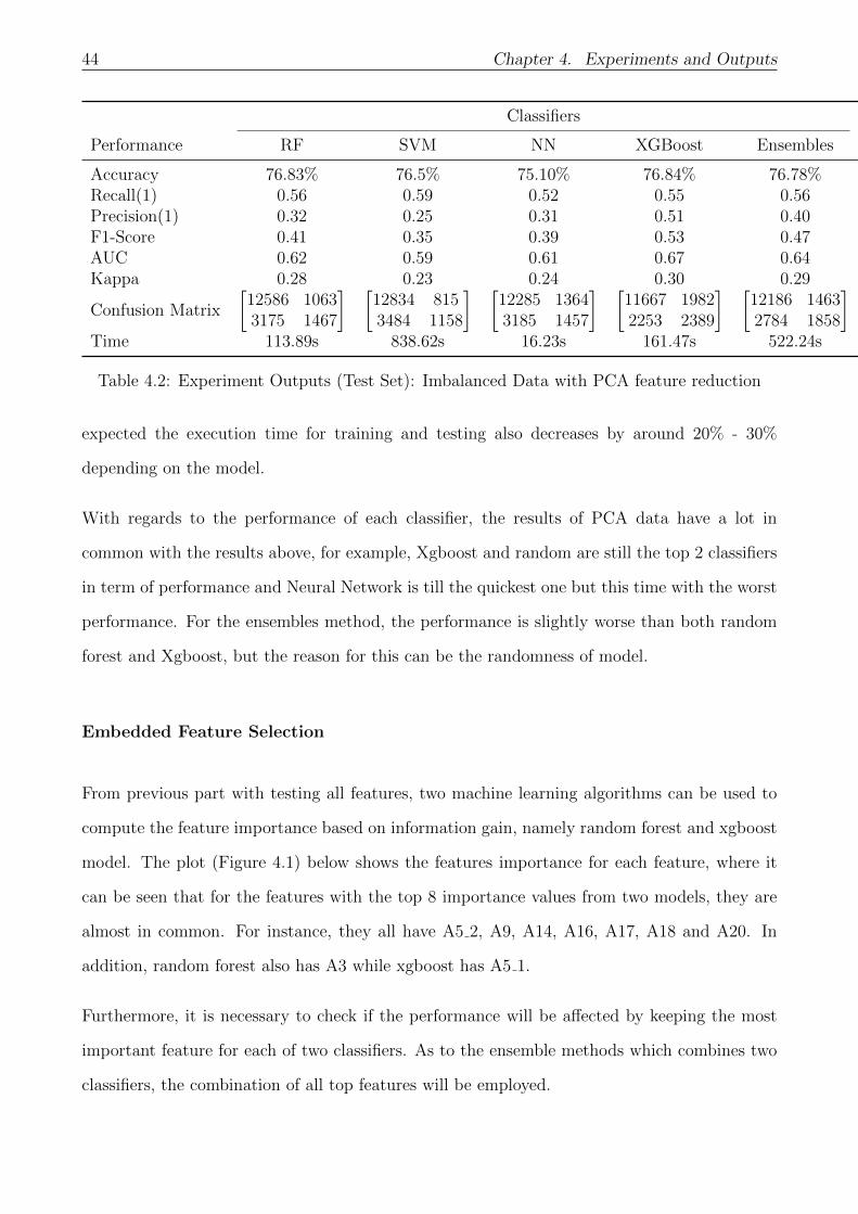
44 Chapter 4. Experiments and Outputs
Classifiers
Performance RF SVM NN XGBoost Ensembles
Accuracy 76.83% 76.5% 75.10% 76.84% 76.78%Recall(1) 0.56 0.59 0.52 0.55 0.56Precision(1) 0.32 0.25 0.31 0.51 0.40F1-Score 0.41 0.35 0.39 0.53 0.47AUC 0.62 0.59 0.61 0.67 0.64Kappa 0.28 0.23 0.24 0.30 0.29
Confusion Matrix
[12586 10633175 1467
] [12834 8153484 1158
] [12285 13643185 1457
] [11667 19822253 2389
] [12186 14632784 1858
]Time 113.89s 838.62s 16.23s 161.47s 522.24s
Table 4.2: Experiment Outputs (Test Set): Imbalanced Data with PCA feature reduction
expected the execution time for training and testing also decreases by around 20% - 30%
depending on the model.
With regards to the performance of each classifier, the results of PCA data have a lot in
common with the results above, for example, Xgboost and random are still the top 2 classifiers
in term of performance and Neural Network is till the quickest one but this time with the worst
performance. For the ensembles method, the performance is slightly worse than both random
forest and Xgboost, but the reason for this can be the randomness of model.
Embedded Feature Selection
From previous part with testing all features, two machine learning algorithms can be used to
compute the feature importance based on information gain, namely random forest and xgboost
model. The plot (Figure 4.1) below shows the features importance for each feature, where it
can be seen that for the features with the top 8 importance values from two models, they are
almost in common. For instance, they all have A5 2, A9, A14, A16, A17, A18 and A20. In
addition, random forest also has A3 while xgboost has A5 1.
Furthermore, it is necessary to check if the performance will be affected by keeping the most
important feature for each of two classifiers. As to the ensemble methods which combines two
classifiers, the combination of all top features will be employed.
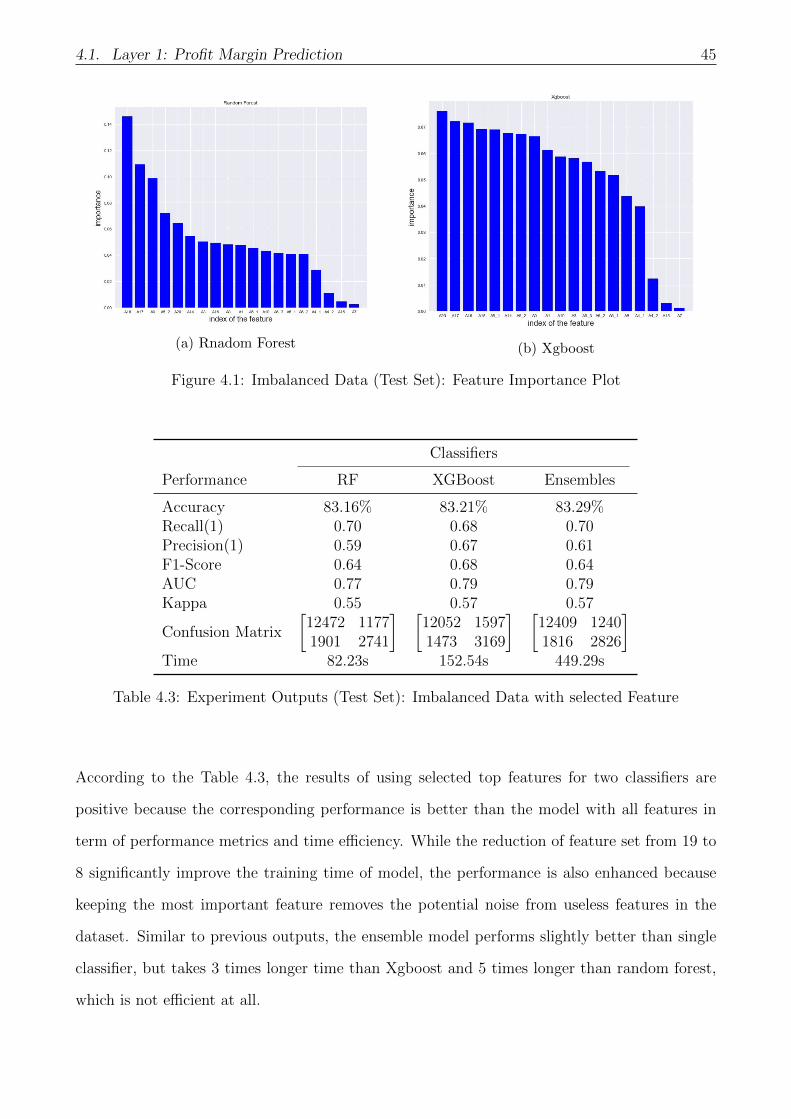
4.1. Layer 1: Profit Margin Prediction 45
(a) Rnadom Forest (b) Xgboost
Figure 4.1: Imbalanced Data (Test Set): Feature Importance Plot
Classifiers
Performance RF XGBoost Ensembles
Accuracy 83.16% 83.21% 83.29%Recall(1) 0.70 0.68 0.70Precision(1) 0.59 0.67 0.61F1-Score 0.64 0.68 0.64AUC 0.77 0.79 0.79Kappa 0.55 0.57 0.57
Confusion Matrix
[12472 11771901 2741
] [12052 15971473 3169
] [12409 12401816 2826
]Time 82.23s 152.54s 449.29s
Table 4.3: Experiment Outputs (Test Set): Imbalanced Data with selected Feature
According to the Table 4.3, the results of using selected top features for two classifiers are
positive because the corresponding performance is better than the model with all features in
term of performance metrics and time efficiency. While the reduction of feature set from 19 to
8 significantly improve the training time of model, the performance is also enhanced because
keeping the most important feature removes the potential noise from useless features in the
dataset. Similar to previous outputs, the ensemble model performs slightly better than single
classifier, but takes 3 times longer time than Xgboost and 5 times longer than random forest,
which is not efficient at all.

46 Chapter 4. Experiments and Outputs
4.1.2 Balanced Data
Since the original dataset has imbalanced problem where minority class only accounts for around
25%, it may have negative influence on the performance on the classifier as mentioned in section
3.3.5. Therefore, in this part, the performance of classifier will be tested, by training the model
on balanced data with three different re-sampling methods, namely oversampling-SMOTE,
undersampling-ENN and combined method-SMOTEENN.
All Features: Scaled Data
Similar to the part mentioned earlier, all features will be used for tested for the performance
of classifier. The only difference is that three types of balanced dataset is used for training the
classifier.
On the basis of tables below (Table 4.4, 4.5 and 4.6), it can be found that the undersampling
methods is the best among other two reassembling methods as the overall performance of all
classifiers in term of Accuracy, F1-Score, AUC and Kappa is better. While the edited nearest
neighbour method reduces the total number of small trades (see Figure 3.10) which helps
classifier mitigate the bias towards the majority class and thus improve the performance, the
other two methods increase the sample of minority class which negatively affects the output of
classifiers especially the combined methods. On the other hand, the increase in minority class
also raises the processing time of models, where in the worst case of SVM the total time is
almost 50 minutes.
In term of model performance, as usual XGBoost and random forest are still the top 2 comparing
to other three classifiers by taking performance metrics and time into considerations. However,
there is one thing should be pointed out that although the accuracy is around 1% lower than
the model without resampling (See Table 4.1), but the performance is better in term of AUC,
F1-Score or Kappa since there is imbalanced class problem in the dataset.
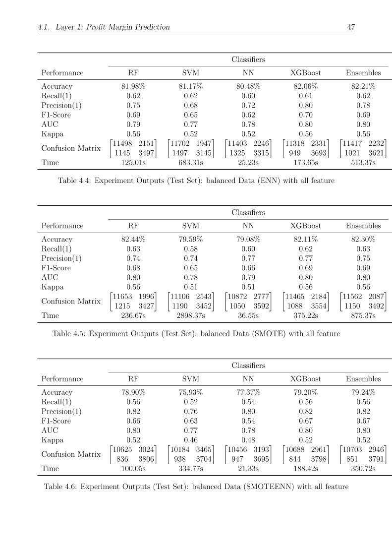
4.1. Layer 1: Profit Margin Prediction 47
Classifiers
Performance RF SVM NN XGBoost Ensembles
Accuracy 81.98% 81.17% 80.48% 82.06% 82.21%Recall(1) 0.62 0.62 0.60 0.61 0.62Precision(1) 0.75 0.68 0.72 0.80 0.78F1-Score 0.69 0.65 0.62 0.70 0.69AUC 0.79 0.77 0.78 0.80 0.80Kappa 0.56 0.52 0.52 0.56 0.56
Confusion Matrix
[11498 21511145 3497
] [11702 19471497 3145
] [11403 22461325 3315
] [11318 2331949 3693
] [11417 22321021 3621
]Time 125.01s 683.31s 25.23s 173.65s 513.37s
Table 4.4: Experiment Outputs (Test Set): balanced Data (ENN) with all feature
Classifiers
Performance RF SVM NN XGBoost Ensembles
Accuracy 82.44% 79.59% 79.08% 82.11% 82.30%Recall(1) 0.63 0.58 0.60 0.62 0.63Precision(1) 0.74 0.74 0.77 0.77 0.75F1-Score 0.68 0.65 0.66 0.69 0.69AUC 0.80 0.78 0.79 0.80 0.80Kappa 0.56 0.51 0.51 0.56 0.56
Confusion Matrix
[11653 19961215 3427
] [11106 25431190 3452
] [10872 27771050 3592
] [11465 21841088 3554
] [11562 20871150 3492
]Time 236.67s 2898.37s 36.55s 375.22s 875.37s
Table 4.5: Experiment Outputs (Test Set): balanced Data (SMOTE) with all feature
Classifiers
Performance RF SVM NN XGBoost Ensembles
Accuracy 78.90% 75.93% 77.37% 79.20% 79.24%Recall(1) 0.56 0.52 0.54 0.56 0.56Precision(1) 0.82 0.76 0.80 0.82 0.82F1-Score 0.66 0.63 0.54 0.67 0.67AUC 0.80 0.77 0.78 0.80 0.80Kappa 0.52 0.46 0.48 0.52 0.52
Confusion Matrix
[10625 3024836 3806
] [10184 3465938 3704
] [10456 3193947 3695
] [10688 2961844 3798
] [10703 2946851 3791
]Time 100.05s 334.77s 21.33s 188.42s 350.72s
Table 4.6: Experiment Outputs (Test Set): balanced Data (SMOTEENN) with all feature
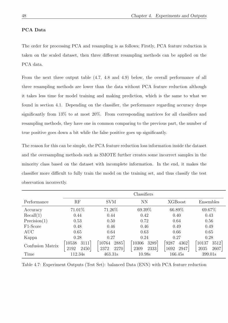
48 Chapter 4. Experiments and Outputs
PCA Data
The order for processing PCA and resampling is as follows; Firstly, PCA feature reduction is
taken on the scaled dataset, then three different resampling methods can be applied on the
PCA data.
From the next three output table (4.7, 4.8 and 4.9) below, the overall performance of all
three resampling methods are lower than the data without PCA feature reduction although
it takes less time for model training and making prediction, which is the same to what we
found in section 4.1. Depending on the classifier, the performance regarding accuracy drops
significantly from 13% to at most 20%. From corresponding matrices for all classifiers and
resampling methods, they have one in common comparing to the previous part, the number of
true positive goes down a bit while the false positive goes up significantly.
The reason for this can be simple, the PCA feature reduction loss information inside the dataset
and the oversampling methods such as SMOTE further creates some incorrect samples in the
minority class based on the dataset with incomplete information. In the end, it makes the
classifier more difficult to fully train the model on the training set, and thus classify the test
observation incorrectly.
Classifiers
Performance RF SVM NN XGBoost Ensembles
Accuracy 71.01% 71.26% 69.39% 66.89% 69.67%Recall(1) 0.44 0.44 0.42 0.40 0.43Precision(1) 0.53 0.50 0.72 0.64 0.56F1-Score 0.48 0.46 0.46 0.49 0.49AUC 0.65 0.64 0.63 0.66 0.65Kappa 0.28 0.27 0.24 0.27 0.28
Confusion Matrix
[10538 31112192 2450
] [10764 28852372 2270
] [10306 32892309 2333
] [9287 43621692 2947
] [10137 35122035 2607
]Time 112.34s 463.31s 10.98s 166.45s 399.01s
Table 4.7: Experiment Outputs (Test Set): balanced Data (ENN) with PCA feature reduction
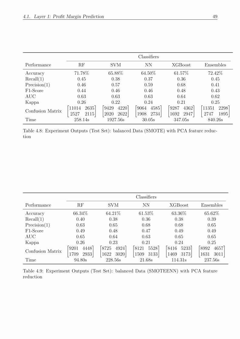
4.1. Layer 1: Profit Margin Prediction 49
Classifiers
Performance RF SVM NN XGBoost Ensembles
Accuracy 71.78% 65.88% 64.50% 61.57% 72.42%Recall(1) 0.45 0.38 0.37 0.36 0.45Precision(1) 0.46 0.57 0.59 0.68 0.41F1-Score 0.44 0.46 0.46 0.48 0.43AUC 0.63 0.63 0.63 0.64 0.62Kappa 0.26 0.22 0.24 0.21 0.25
Confusion Matrix
[11014 26352527 2115
] [9429 42202020 2622
] [9064 45851908 2734
] [9287 43621692 2947
] [11351 22982747 1895
]Time 258.14s 1927.56s 30.05s 347.05s 840.26s
Table 4.8: Experiment Outputs (Test Set): balanced Data (SMOTE) with PCA feature reduc-tion
Classifiers
Performance RF SVM NN XGBoost Ensembles
Accuracy 66.34% 64.21% 61.53% 63.36% 65.62%Recall(1) 0.40 0.38 0.36 0.38 0.39Precision(1) 0.63 0.65 0.68 0.68 0.65F1-Score 0.49 0.48 0.47 0.49 0.49AUC 0.65 0.64 0.63 0.65 0.65Kappa 0.26 0.23 0.21 0.24 0.25
Confusion Matrix
[9201 44481709 2933
] [8725 49241622 3020
] [8121 55281509 3133
] [8416 52331469 3173
] [8992 46571631 3011
]Time 94.80s 228.56s 21.68s 114.31s 237.56s
Table 4.9: Experiment Outputs (Test Set): balanced Data (SMOTEENN) with PCA featurereduction
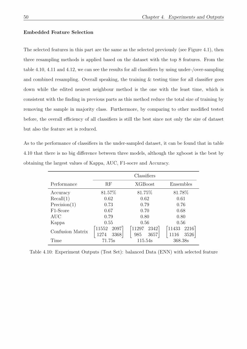
50 Chapter 4. Experiments and Outputs
Embedded Feature Selection
The selected features in this part are the same as the selected previously (see Figure 4.1), then
three resampling methods is applied based on the dataset with the top 8 features. From the
table 4.10, 4.11 and 4.12, we can see the results for all classifiers by using under-/over-sampling
and combined resampling. Overall speaking, the training & testing time for all classifier goes
down while the edited nearest neighbour method is the one with the least time, which is
consistent with the finding in previous parts as this method reduce the total size of training by
removing the sample in majority class. Furthermore, by comparing to other modified tested
before, the overall efficiency of all classifiers is still the best since not only the size of dataset
but also the feature set is reduced.
As to the performance of classifiers in the under-sampled dataset, it can be found that in table
4.10 that there is no big difference between three models, although the xgboost is the best by
obtaining the largest values of Kappa, AUC, F1-socre and Accuracy.
Classifiers
Performance RF XGBoost Ensembles
Accuracy 81.57% 81.75% 81.78%Recall(1) 0.62 0.62 0.61Precision(1) 0.73 0.79 0.76F1-Score 0.67 0.70 0.68AUC 0.79 0.80 0.80Kappa 0.55 0.56 0.56
Confusion Matrix
[11552 20971274 3368
] [11297 2342985 3657
] [11433 22161116 3526
]Time 71.75s 115.54s 368.38s
Table 4.10: Experiment Outputs (Test Set): balanced Data (ENN) with selected feature
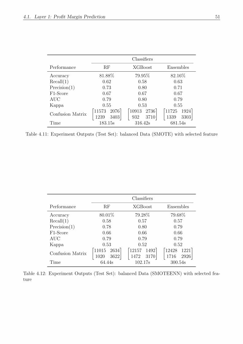
4.1. Layer 1: Profit Margin Prediction 51
Classifiers
Performance RF XGBoost Ensembles
Accuracy 81.88% 79.95% 82.16%Recall(1) 0.62 0.58 0.63Precision(1) 0.73 0.80 0.71F1-Score 0.67 0.67 0.67AUC 0.79 0.80 0.79Kappa 0.55 0.53 0.55
Confusion Matrix
[11573 20761239 3403
] [10913 2736932 3710
] [11725 19241339 3303
]Time 183.15s 316.42s 681.54s
Table 4.11: Experiment Outputs (Test Set): balanced Data (SMOTE) with selected feature
Classifiers
Performance RF XGBoost Ensembles
Accuracy 80.01% 79.28% 79.68%Recall(1) 0.58 0.57 0.57Precision(1) 0.78 0.80 0.79F1-Score 0.66 0.66 0.66AUC 0.79 0.79 0.79Kappa 0.53 0.52 0.52
Confusion Matrix
[11015 26341020 3622
] [12157 14921472 3170
] [12428 12211716 2926
]Time 64.44s 102.17s 300.54s
Table 4.12: Experiment Outputs (Test Set): balanced Data (SMOTEENN) with selected fea-ture
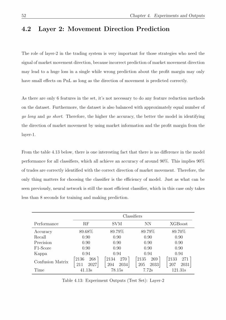
52 Chapter 4. Experiments and Outputs
4.2 Layer 2: Movement Direction Prediction
The role of layer-2 in the trading system is very important for those strategies who need the
signal of market movement direction, because incorrect prediction of market movement direction
may lead to a huge loss in a single while wrong prediction about the profit margin may only
have small effects on PnL as long as the direction of movement is predicted correctly.
As there are only 6 features in the set, it’s not necessary to do any feature reduction methods
on the dataset. Furthermore, the dataset is also balanced with approximately equal number of
go long and go short. Therefore, the higher the accuracy, the better the model in identifying
the direction of market movement by using market information and the profit margin from the
layer-1.
From the table 4.13 below, there is one interesting fact that there is no difference in the model
performance for all classifiers, which all achieve an accuracy of around 90%. This implies 90%
of trades are correctly identified with the correct direction of market movement. Therefore, the
only thing matters for choosing the classifier is the efficiency of model. Just as what can be
seen previously, neural network is still the most efficient classifier, which in this case only takes
less than 8 seconds for training and making prediction.
Classifiers
Performance RF SVM NN XGBoost
Accuracy 89.68% 89.79% 89.79% 89.70%Recall 0.90 0.90 0.90 0.90Precision 0.90 0.90 0.90 0.90F1-Score 0.90 0.90 0.90 0.90Kappa 0.94 0.94 0.94 0.94
Confusion Matrix
[2136 268211 2027
] [2134 270204 2034
] [2135 269205 2033
] [2133 271207 2031
]Time 41.13s 78.15s 7.72s 121.31s
Table 4.13: Experiment Outputs (Test Set): Layer-2

4.3. Performance of Combining Two Layers 53
4.3 Performance of Combining Two Layers
As mentioned in section 3.2 (also see Figure 3.1), the two layers work in the following order;
in the beginning the layer-1 receives the request from the strategy to make prediction on the
profit margin and then it send another request to the layer-2 for determining the movement
direction. If the profit margin is identified as small by the layer-1, the layer-2 will directly
send this signal back to the strategy and tell them to not participate in the trade. However,
if the margin is big, the layer-2 will immediately start processing to make prediction on the
movement direction by using current market information and then send back the signal of go
long or go short based on the prediction.
Based on the results, for the layer-1 Xgboost is the only selected classifier due to its high per-
formance, but two datasets are used for training the model, namely standardized dataset with
selected features (embedded feature selection) and undersampling dataset also with selected
feature. With respect to the second layer, neural network is chosen because of its high effi-
ciency. For the purpose of measuring overall performance of how the two layers work together,
both performance metrics and profitability analysis will be tested in this part.
The table 4.14 shows the output of two combinations of layers. In term of statistical performance
metrics such as Accuracy, Precision and F1-Score, it can be found that the combination of
Xgboost without using resampling and Neural Network performs better than the its competitor,
since in the first layer it predicts less incorrect small trades (true small → predicted big).
However, as to the profitability improvement in trading strategy, the one with using balanced
data gains 12% profit than another one, which is mainly due to the fact it predicts more correct
big trades ((true big → predicted big)) although more incorrect small trades are made.
By further checking the composition of Profit and Loss for each combination of layers, there is
an interesting fact should be mentioned that the second combination of filters did around 45%
more incorrect trades than the first combination, but it generates around 50% more profit from
doing these incorrect small trades. The reason can be that the layers is also good at predicting
the direction of movement even if the potential profit margin is small. However, it cannot be
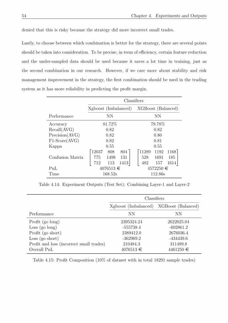
54 Chapter 4. Experiments and Outputs
denied that this is risky because the strategy did more incorrect small trades.
Lastly, to choose between which combination is better for the strategy, there are several points
should be taken into consideration. To be precise, in term of efficiency, certain feature reduction
and the under-sampled data should be used because it saves a lot time in training, just as
the second combination in our research. However, if we care more about stability and risk
management improvement in the strategy, the first combination should be used in the trading
system as it has more reliability in predicting the profit margin.
Classifiers
Xgboost (Imbalanced) XGBoost (Balanced)
Performance NN NN
Accuracy 81.72% 79.78%Recall(AVG) 0.82 0.82Precision(AVG) 0.82 0.80F1-Score(AVG) 0.82 0.81Kappa 0.55 0.55
Confusion Matrix
12037 808 804775 1498 131712 113 1413
11289 1192 1168528 1691 185482 157 1614
PnL 4076513 e 4572250 eTime 168.52s 112.86s
Table 4.14: Experiment Outputs (Test Set): Combining Layer-1 and Layer-2
Classifiers
Xgboost (Imbalanced) XGBoost (Balanced)
Performance NN NN
Profit (go long) 2395324.24 2622025.04Loss (go long) -555738.4 -602861.2Profit (go short) 2389412.0 2676036.4Loss (go short) -362969.2 -434439.6Profit and loss (incorrect small trades) 210484.3 311489.8Overall PnL 4076513 e 4461250 e
Table 4.15: Profit Composition (10% of dataset with in total 18291 sample trades)
Chapter 5
Conclusion
As the technology develops, trading is now becoming a more and more complex process where
the financial markets keep getting faster and the volumes of trading data keep escalating.
Machine Learning or data mining can provide the potential to give traders an edge by spotting
or predicting trends.
This paper explores the problem of predicting profit margin (of potential trade) and market
movement direction in the short term (less than one minute) in the future by apply ting machine
learning techniques, with the practical purpose of building filters to improve the stability and
profitability of algorithmic trading strategy in the system. Although this is a popular topic
in both trading industry and academia and a lot of effort has been put into research, limited
results/papers are available in the public as the intention for the company or research to publish
the results is extremely low given the high competition in the industry.
The chapter 2 mainly provides a general introduction to machine learning that used in this
research including some of supervised machine learning classification algorithms like random
forest and xgboost, performance evaluation metrics such as F1-Score, AUC and profitability
analysis and lastly the model validation. As discussed in this chapter, the main goal of this
research is not for designing a independent trading algorithm based on machine learning but
to build a decision filter for the trading strategies to help them in better analyzing market
55

56 Chapter 5. Conclusion
information and make trading decision with the help of strong power in machine learning.
The chapter 3 discusses two topics. The first topic is mainly about the framework of two filters
and its role and relationship with other components such as trading algorithm in the system.
The second topics talks about the data engineering methods in accordance with the problem
we have in the datasets, such as different scale of features, similar features and imbalanced
class. Some methods are applied to try to solve the issue in the dataset, for instance, the
PCA/Embedded feature reduction is utilized to reduce the useless feature while resampling
techniques such as SMOTE is applied to make the two classes more balanced.
5.1 Summary of Thesis Achievements
The chapter 4 reports the outputs of layer-1, layer-2 and combined layer system with using
different combinations of machine learning algorithms and modified datasets, in term of sta-
tistical performance metrics and profitability. In the end, two top combinations of layers are
chosen where one of them has better performance in statistical performance and the other one
is good at improving the profitability of trading algorithms and spend less in training and make
predictions.
To be more specific, for the combined filter with using xgboost classifier and Neural network
on scaled dataset with embedded feature reduction, the filter achieves an accuracy of 81.72%
and the same level of precision, recall and f1-score. In the first layer, approximately 70% of
big trades are correctly classified and around 90% of them are then predicted with the correct
direction in the second layers. For those miss-classified small trades, the direction can also
be mostly classified correctly by achieving a positive profit. For another combined with using
the same classifiers but on the under-sampled dataset with selected features, the statistical
performance is bit lower than the previous one with accuracy around 80%. However, in term
of PnL, this filter is better since more true big trades are predicted and executed and further
the extra classified small trades also generate extra profit to overall PnL. Lastly, with regard
5.2. Future Work 57
to the efficiency, it is found that the second combined filter spends 50% less time than the first
combined filter as the size of dataset is reduced by undersampling.
Both two filters are useful for trading algorithms, especially for momentum trading based
strategy, which help the strategy or trader better analyze significant market movements in one
direction on high volume with help of machine learning algorithms.
5.2 Future Work
There are several aspects in this research can be improved in future work. Firstly, the re-
sult/performance of this two-layer filter can be improved, especially in the first layer. As the
classifier has some difficulty in identifying the trades with profit margin nearby 30 BPS based
on current feature set, some trades are thus misclassified as small or big trades which has big
influence on the final PnL. The possible solution is to improve the quality of feature set, for
example, by adding some new useful features in identifying the profit margin.
Secondly, with respect to the efficiency, the xgboost classifier takes too much time in model
training and making prediction, comparing to neural network. Therefore, neural network or
enhanced version of neural network (deep neural network/deep learning) can be a good try to
improve the efficiency as long as there is enough good-quality feature set.
Lastly, although in this research the main purpose is not to build a independent trading strategy
based on machine learning, this can be future direction of research. By further incorporating
the risk management and market perception, an independent strategy can be developed with
help of machine learning.

Bibliography
[1] E. F. Fama. The behavior of stock-market prices. Journal of Business, 38(1), 1965
[2] Victor Lavrenko, Matt Schmill, Dawn Lawrie, Paul Ogilvie, David Jensen, and James Al-
lan.: Language models for financial news recommendation. In Proceedings of the ninth In-
ternational Conference on Information and Knowledge Management, pages 389396. ACM,
2000.
[3] Cheng-Lung Huang and Cheng-Yi Tsai.: A hybrid SOFM-SVR with a filter based feature
selection for stock market forecasting. Expert Systems with Applications, 36(2, Part 1):1529
1539, 2009.
[4] Wei Shen, Xiaopen Guo, Chao Wu, and Desheng Wu. Forecasting stock indices using radial
basis function neural networks optimized by artificial fish swarm algorithm. Knowledge-
Based Systems, 24(3):378385, 2011.
[5] Marco Lippi, Lorenzo Menconi, and Marco Gori. Balancing recall and precision in stock
market predictors using support vector machines. In Neural Nets and Surroundings, pages
5158. Springer, 2013.
[6] Yu, Lean, Huanhuan Chen, Shouyang Wang, and Kin Keung Lai.: Evolving Least Squares
Support Vector Machines for Stock Market Trend Mining. IEEE Transactions on Evolu-
tionary Computation. Vol 13. no 1. Feb (2009): 87-102.
[7] Lahmiri, Salim. A Comparison of PNN and SVM for Stock Market Trend Prediction us-
58
BIBLIOGRAPHY 59
ing Economic and Technical Information. International Journal of Computer Applications
(0975 8887). Vol 29, No 3 Sept (2011): 24-30
[8] Corrina Cortes and Vladimir Vapinik.: Support Vector Network ; 1995
[9] Vladimir Vapnik. The Nature of Statistical Learning Theory. Springer, 1995
[10] Anthony Brabazon and Michael ONeill. Biologically Inspired Algorithms for Financial
Modelling, volume 20. Springer Berlin, 2006
[11] Paul A Weller, Geoffrey C Friesen, and Lee M Dunham. Price trends and patterns in
technical analysis: A theoretical and empirical examination. Journal of Banking Finance,
33(6):10891100, 2009
[12] Breiman, L., Random Forests. Machine Learning, 45(1), pp.532, 2001
[13] Jerome H. Friedman, Greedy Function Approximation: A Gradient Boosting Machine,
1999
[14] Wolpert, D., Stacked Generalization, Neural Networks, 5(2), pp. 241-259., 1992
[15] Breiman, L., Stacked Regression, Machine Learning, , 24, 1996
[16] Ozay, M.; Yarman Vural, F. T. . A New Fuzzy Stacked Generalization Technique and
Analysis of its Performance., 2013
[17] Robert P Schumaker and Hsinchun Chen.: A quantitative stock prediction system based on
financial news. Information Processing Management, 45(5):571 583, 2009.
[18] Arie Ben-David.: About the relationship between ROC curves and Cohens kappa. Engineer-
ing Applications of Artificial Intelligence, 21(6):874882, 2008.
[19] Stephan Schulmeister.: Profitability of technical stock trading: Has it moved from daily to
intraday data? Review of Financial Economics, 18(4):190201, 2009.
60 BIBLIOGRAPHY
[20] LA Teixeira, ALI De Oliveira: A method for automatic stock trading combining techni-
cal analysis and nearest neighbor classification. Expert systems with applications, 2010 -
Elsevier
[21] Lamartine Almeida Teixeira and Adriano Lorena Inacio De Oliveira.: A method for auto-
matic stock trading combining technical analysis and nearest neighbor classification. Expert
Systems with Applications, 37(10):68856890, 2010.
[22] Tao Wang and Jian Yang. Nonlinearity and intraday efficiency tests on energy futures
markets. Energy Economics, 32(2):496503, 2010.
[23] Bing Liu.: Web Data Mining: Exploring Hyperlinks, Contents, and Usage Data. Springer
Verlag, 2011
[24] Michael Steinbach, Tan Pang-Ning and Vipin Kumar.: Introduction to Data Mining.
Addison-Wesley, 2005
[25] Mohamed Gaber, Arkady Zaslavsky, and Shonali Krishnaswamy.: A survey of classification
methods in data streams. in Data Streams: Models and Algorithms, pages 3959, 2007.
[26] V. Kapoor, A.P. Khurana, S. Der.: Genetic Algorithm: An Application to Technical Trad-
ing System Design. International Journal of Computer Applications (0975 8887) Volume
36 No.5, December 2011
[27] Dorian Pyle. Data Preparation for Data Mining, volume 1. Morgan Kaufmann Publishers,
Inc., 1999
[28] Ajoy K Palit and Dobrivoje Popovic.: Computational Intelligence in Time Series Fore-
casting: Theory and Engineering Applications (Advances in Industrial Control). Springer-
Verlag New York, Inc., Secaucus, NJ, 2005.
[29] Koch, R., The 80/20 Principle: The Secret of Achieving More with Less, London: Nicholas
Brealey Publishing, 2001
BIBLIOGRAPHY 61
[30] Zwillinger, D. and Kokoska, S. CRC Standard Probability and Statistics Tables and For-
mulae. Chapman Hall: New York. 2000
[31] Kyoung-jae Kim and Ingoo Han. Genetic algorithms approach to feature discretization
in artificial neural networks for the prediction of stock price index. Expert Systems with
Applications,19(2):125132, 2000.
[32] Smith Lindsay.:”A tutorial on Principal Components Analysis. University of Otago, De-
partment of Computer Science, 2002
[33] John H Holland. Genetic algorithms. Scientific American, 267(1):6672, 1992.
[34] Thomas Navin Lal, Olivier Chapelle, Jason Weston, and Andre Elisseeff. Embedded meth-
ods. In Feature Extraction, pages 137165. Springer, 2006
[35] Yvan Saeys, Inaki Inza, and Pedro Larranaga. A review of feature selection techniques in
bioinformatics. Bioinformatics, 23(19):25072517, 2007.
[36] Victoria Lopez, Alberto Fernandez, Jose G Moreno-Torres, and Francisco Herrera. Analysis
of preprocessing vs. cost-sensitive learning for imbalanced classification open problems on
intrinsic data characteristics. Expert Systems with Applications, 39(7):65856608, 2012.
[37] Nitesh V. Chawla, Kevin W. Bowyer, Lawrence O. Hall and W. Philip Kegelmeyer.
SMOTE: Synthetic Minority Over-sampling Technique. Journal of Artificial Intelligence
Research 16 (2002) 321357, 2002.
[38] D. Wilson, Asymptotic Properties of Nearest Neighbor Rules Using Edited Data. In IEEE
Transactions on Systems, Man, and Cybernetrics, vol. 2 (3), pp. 408-421, 1972.
[39] J. Laurikkala, Improving identification of difficult small classes by balancing class distri-
bution. Springer Berlin Heidelberg, 2001.
[40] M. Kubat, S. Matwin, Addressing the curse of imbalanced training sets: one-sided selection.
In ICML, vol. 97, pp. 179-186, 1997

62 BIBLIOGRAPHY
[41] I. Tomek, Two modifications of CNN, In Systems, Man, and Cybernetics. IEEE Transac-
tions on, vol. 6, pp 769-772, 2010
[42] G. Batista, R. C. Prati, M. C. Monard. A study of the behavior of several methods for
balancing machine learning training data. ACM Sigkdd Explorations Newsletter 6 (1),
20-29, 2004
[43] A. Timmermann.: Elusive return predictability. International Journal of Forecasting,
24(1):118, 2008.
[44] Barry Johnson.: Algorithmic Trading & DMA: An Introduction to direct access trading
strategies. 4Myeloma Press, 2010.

Chapter 6
Appendix
Trade-1 Trade-2initial side buy selltotalqty 67000 22700Avg. Price 371 5275end side sell buytotalqty 67000 22700Avg. Price 369.67 5246.67pnljpy -72000 639300pnleur -576 5114.4Percentage -0.00289 0.00534Basis Point -28.9 53.4Profti Margin 0-small 1-bigDirection 0-no action 2-sell
Table 6.1: Example Trade
63

64 Chapter 6. Appendix
Feature DefinitionA1 AnonymousA2 AnonymousA3 AnonymousA4 1 High-low difference in 5 minsA4 2 High-low difference in 10 minsA5 1 AnonymousA5 2 AnonymousA6 1 Moving Average in 5 minsA6 2 Moving Average in 10 minsA6 3 Moving Average in 30 minsA7 Binary: whether within 5 mins of market openA8 AnonymousA9 AnonymousA10 AnonymousA11 AnonymousA12 AnonymousA13 Measurement of Tick SizeA14 Recent VolatilityA15 AnonymousA16 History VolatilityA17 One minute Trading VolumeA18 SpreadA19 Anonymous
Table 6.2: Feature Table


![K-theory Classi cations for Symmetry-Protected …In his pioneering work [42], Kitaev classi es symmetry-protected topological phases of free fermions for some important symmetry groups,](https://img.pdfslide.us/doc/110x75/5f0542bb7e708231d41214d3/k-theory-classi-cations-for-symmetry-protected-in-his-pioneering-work-42-kitaev.jpg)


![Research Article Cryptanalytic Performance Appraisal of ...downloads.hindawi.com/journals/mpe/2014/429271.pdf · Lee et al. [ ] provide new classi cations of proxy sig-nature scheme,](https://img.pdfslide.us/doc/110x75/6027108a5a3b656d3f798bcd/research-article-cryptanalytic-performance-appraisal-of-lee-et-al-provide.jpg)