Embed Size (px)
Citation preview

Machine Learning: Chenhao TanUniversity of Colorado BoulderLECTURE 8
Slides adapted from Jordan Boyd-Graber, Justin Johnson, Andrej Karpathy, Chris Ketelsen, Fei-Fei Li, Mike Mozer, Michael Nielson
Machine Learning: Chenhao Tan | Boulder | 1 of 53

HW1 grades
• Most people did well!• We are extra lenient this time• Submit only your code in a zip file, with no folder structure
Machine Learning: Chenhao Tan | Boulder | 2 of 53

Final projects
• Team formation
Machine Learning: Chenhao Tan | Boulder | 3 of 53

Quiz 1
Which of the following statements is true? (Suppose that training data is large.)A. In training, K-nearest neighbors takes shorter time than neural networks.B. In training, K-nearest neighbors takes longer time than neural networks.C. In testing, K-nearest neighbors takes shorter time than neural networks.D. In testing, K-nearest neighbors takes longer time than neural networks.
Machine Learning: Chenhao Tan | Boulder | 4 of 53

Quiz 2
How many parameters are there in the following feed-forward neural networks(assuming no biases)?
x1
x2
. . .
x100
h1
. . .
h50
h1
. . .
h20
o1
. . .
o5
A. 100 * 50 + 50 * 20 + 20 * 5B. 100 * 50 + 50 + 50 * 20 + 20 + 20 * 5 + 5
Machine Learning: Chenhao Tan | Boulder | 5 of 53

Quiz 3
How many parameters are there in the following convolutional neural networks?(assuming no biases, convolution with 4 filters, max pooling, ReLu, and finally afully-connected layer)
input image (10*10)
4 filters 5*5, stride 1
4@6*6
Max pooling 2*2, stride 2
4@3*3 5*1
Machine Learning: Chenhao Tan | Boulder | 6 of 53

Quiz 3
How many ReLU operations are performed on the forward pass? (assuming nobiases, convolution with 4 filters, max pooling, ReLu, and finally a fully-connectedlayer)
input image (10*10)
4 filters 5*5, stride 1
4@6*6
Max pooling 2*2, stride 2
4@3*3 5*1
Machine Learning: Chenhao Tan | Boulder | 6 of 53

Overview
History lesson
Deep learning in practiceImprove stochastic gradient descentUnstable gradientsData preprocessingWeight InitializationModel Architecture
Machine Learning: Chenhao Tan | Boulder | 7 of 53

History lesson
Outline
History lesson
Deep learning in practiceImprove stochastic gradient descentUnstable gradientsData preprocessingWeight InitializationModel Architecture
Machine Learning: Chenhao Tan | Boulder | 8 of 53

History lesson
History lesson
• 1962: Rosenblatt, Principles of Neurodynamics: Perceptrons and the Theory ofBrain Mechanisms◦ First neuron-based learning algorithm◦ “Could learning anything that you could program”
• 1969: Minsky & Papert, Perceptron: An Introduction to ComputationalGeometry◦ First real complexity analysis◦ Showed, in principle, many things that perceptrons can’t learn to do◦ Shut down any interest in neural networks
Machine Learning: Chenhao Tan | Boulder | 9 of 53

History lesson
History lesson
• 1986: Rumelhart, Hinton & Williams, Back Propagation◦ Overcame many difficulties raised by Minsky et al.◦ Neural networks wildly popular again (for a while)
Machine Learning: Chenhao Tan | Boulder | 10 of 53

History lesson
History lesson
• 1999-2005◦ Shift to Bayesian Methods
• Best ideas from neural networks• Direct statistical computing
◦ Support Vector Machines• Nice mathematical properties• Kernel tricks
◦ A few people still playing with NNs• Bengio• Hinton• LeCun
Machine Learning: Chenhao Tan | Boulder | 11 of 53

History lesson
History lesson
• 2005-2010◦ Core group continues to make improvements◦ Various tricks to make NNs practical
• 2010-present◦ BOOM!
Machine Learning: Chenhao Tan | Boulder | 12 of 53

History lesson
AlexNet
Krizhevsky et al. [2012]
Machine Learning: Chenhao Tan | Boulder | 13 of 53

History lesson
History lesson
Question: Why? What made neural networks amazing again?• Massive datasets• Computing power• Algorithmic improvements
Machine Learning: Chenhao Tan | Boulder | 14 of 53

History lesson
History lesson
Machine learning has a short history, but seems cyclic.What is next?
Machine Learning: Chenhao Tan | Boulder | 15 of 53

Deep learning in practice
Outline
History lesson
Deep learning in practiceImprove stochastic gradient descentUnstable gradientsData preprocessingWeight InitializationModel Architecture
Machine Learning: Chenhao Tan | Boulder | 16 of 53

Deep learning in practice | Improve stochastic gradient descent
Outline
History lesson
Deep learning in practiceImprove stochastic gradient descentUnstable gradientsData preprocessingWeight InitializationModel Architecture
Machine Learning: Chenhao Tan | Boulder | 17 of 53

Deep learning in practice | Improve stochastic gradient descent
Gradient descent
Gradient descentwt+1 = wt − η∇f (wt)
Machine Learning: Chenhao Tan | Boulder | 18 of 53

Deep learning in practice | Improve stochastic gradient descent
AdaGrad
Not all features are created equal!
• Gradient descentwt+1 = wt − η∇f (wt)
• Adagrad [Duchi et al., 2011]
cache = cache + (∇f (wt))2
wt+1 = wt − η1
10−7 +√
cache∇f (wt)
Machine Learning: Chenhao Tan | Boulder | 19 of 53

Deep learning in practice | Improve stochastic gradient descent
AdaGrad
Not all features are created equal!• Gradient descent
wt+1 = wt − η∇f (wt)
• Adagrad [Duchi et al., 2011]
cache = cache + (∇f (wt))2
wt+1 = wt − η1
10−7 +√
cache∇f (wt)
Machine Learning: Chenhao Tan | Boulder | 19 of 53

Deep learning in practice | Improve stochastic gradient descent
AdaGrad
Not all features are created equal!• Gradient descent
wt+1 = wt − η∇f (wt)
• Adagrad [Duchi et al., 2011]
cache = cache + (∇f (wt))2
wt+1 = wt − η1
10−7 +√
cache∇f (wt)
Machine Learning: Chenhao Tan | Boulder | 19 of 53

Deep learning in practice | Improve stochastic gradient descent
Momentum
• Gradient descentwt+1 = wt − η∇f (wt)
Machine Learning: Chenhao Tan | Boulder | 20 of 53

Deep learning in practice | Improve stochastic gradient descent
Momentum
• Gradient descentwt+1 = wt − η∇f (wt)
Physical interpretation: Imagine a object is falling, but it does not accumulateany velocity. Let us fix that!
• Momentum
vt+1 = βvt −∇f (wt)
wt+1 = wt + ηvt+1
Machine Learning: Chenhao Tan | Boulder | 21 of 53
Deep learning in practice | Improve stochastic gradient descent
Momentum
• Gradient descentwt+1 = wt − η∇f (wt)
Physical interpretation: Imagine a object is falling, but it does not accumulateany velocity.
Let us fix that!• Momentum
vt+1 = βvt −∇f (wt)
wt+1 = wt + ηvt+1
Machine Learning: Chenhao Tan | Boulder | 21 of 53

Deep learning in practice | Improve stochastic gradient descent
Momentum
• Gradient descentwt+1 = wt − η∇f (wt)
Physical interpretation: Imagine a object is falling, but it does not accumulateany velocity. Let us fix that!
• Momentum
vt+1 = βvt −∇f (wt)
wt+1 = wt + ηvt+1
Machine Learning: Chenhao Tan | Boulder | 21 of 53

Deep learning in practice | Improve stochastic gradient descent
Momentum
http://cs231n.github.io/assets/nn3/opt2.gifImage credit: Alec Radford
Machine Learning: Chenhao Tan | Boulder | 22 of 53

Deep learning in practice | Improve stochastic gradient descent
More variations
• Adam [Kingma and Ba, 2014]• RMSProp
Machine Learning: Chenhao Tan | Boulder | 23 of 53

Deep learning in practice | Improve stochastic gradient descent
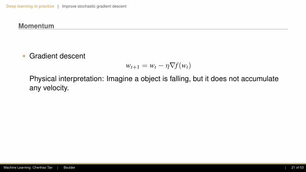
Dropout layer
"randomly set some neurons to zero in the forward pass" [Srivastava et al., 2014]
Machine Learning: Chenhao Tan | Boulder | 24 of 53
Deep learning in practice | Improve stochastic gradient descent
Dropout layer
Forces the network to have a redundantrepresentation
Machine Learning: Chenhao Tan | Boulder | 25 of 53

Deep learning in practice | Improve stochastic gradient descent
Dropout layer
Another interpretation: Dropout is training alarge ensemble of models
Machine Learning: Chenhao Tan | Boulder | 25 of 53

Deep learning in practice | Unstable gradients
Outline
History lesson
Deep learning in practiceImprove stochastic gradient descentUnstable gradientsData preprocessingWeight InitializationModel Architecture
Machine Learning: Chenhao Tan | Boulder | 26 of 53

Deep learning in practice | Unstable gradients
Unstable gradients
x h1 h2 . . . hL o
∂L
∂b1 = σ′(z1)× w2 × σ′(z2)× w3 . . . σ′(zL)∂L
∂aL
Machine Learning: Chenhao Tan | Boulder | 27 of 53

Deep learning in practice | Unstable gradients
Unstable gradients
x h1 h2 . . . hL o
∂L
∂b1 = σ′(z1)× w2 × σ′(z2)× w3 . . . σ′(zL)∂L
∂aL
Machine Learning: Chenhao Tan | Boulder | 27 of 53

Deep learning in practice | Unstable gradients
Unstable gradients
10 0 100.0
0.2
0.4
0.6
0.8
1.0sigmoidderivative
Machine Learning: Chenhao Tan | Boulder | 28 of 53
Deep learning in practice | Unstable gradients
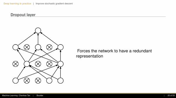
Vanishing gradients
If we use Gaussian initialization for weights, wj ∼ N (0, 1),
|wj| < 1
|wjσ′(zj)| <14
∂L
∂b1 decay to zero exponentially
Machine Learning: Chenhao Tan | Boulder | 29 of 53

Deep learning in practice | Unstable gradients
Vanishing gradients
ReLu
2 0 20.0
0.5
1.0
1.5
2.0ReLuderivative
Machine Learning: Chenhao Tan | Boulder | 30 of 53

Deep learning in practice | Unstable gradients
Exploding gradients
If wj = 100,|wjσ′(zj)| ≈ k > 1
Machine Learning: Chenhao Tan | Boulder | 31 of 53

Deep learning in practice | Data preprocessing
Outline
History lesson
Deep learning in practiceImprove stochastic gradient descentUnstable gradientsData preprocessingWeight InitializationModel Architecture
Machine Learning: Chenhao Tan | Boulder | 32 of 53

Deep learning in practice | Data preprocessing
Another subtle issue of activation function
If all inputs x are positive, thegradients on w are either all positiveor all negative.
Zero-center the inputs!
Machine Learning: Chenhao Tan | Boulder | 33 of 53

Deep learning in practice | Data preprocessing
Another subtle issue of activation function
If all inputs x are positive, thegradients on w are either all positiveor all negative.Zero-center the inputs!
Machine Learning: Chenhao Tan | Boulder | 33 of 53

Deep learning in practice | Data preprocessing
Data preprocessing
Original data
10 5 0 5 1010
5
0
5
10
Zero-centered data(X − X.mean(axis = 0))
10 5 0 5 1010
5
0
5
10
Normalized data(X/ = np.std(X, axis = 0))
10 5 0 5 1010
5
0
5
10
PCA, whitening
Machine Learning: Chenhao Tan | Boulder | 34 of 53

Deep learning in practice | Data preprocessing
Data preprocessing
Original data
10 5 0 5 1010
5
0
5
10
Zero-centered data(X − X.mean(axis = 0))
10 5 0 5 1010
5
0
5
10
Normalized data(X/ = np.std(X, axis = 0))
10 5 0 5 1010
5
0
5
10
PCA, whitening
Machine Learning: Chenhao Tan | Boulder | 34 of 53

Deep learning in practice | Data preprocessing
Data preprocessing
Original data
10 5 0 5 1010
5
0
5
10
Zero-centered data(X − X.mean(axis = 0))
10 5 0 5 1010
5
0
5
10
Normalized data(X/ = np.std(X, axis = 0))
10 5 0 5 1010
5
0
5
10
PCA, whitening
Machine Learning: Chenhao Tan | Boulder | 34 of 53

Deep learning in practice | Data preprocessing
Data preprocessing
Original data
10 5 0 5 1010
5
0
5
10
Zero-centered data(X − X.mean(axis = 0))
10 5 0 5 1010
5
0
5
10
Normalized data(X/ = np.std(X, axis = 0))
10 5 0 5 1010
5
0
5
10
PCA, whitening
Machine Learning: Chenhao Tan | Boulder | 34 of 53

Deep learning in practice | Data preprocessing
Batch normalization
Why only for the input data? [Ioffe and Szegedy, 2015]Consider a batch of activations at some layer. Make each dimension unit gaussian:
ak =ak − E[ak]√
Var[ak]
Machine Learning: Chenhao Tan | Boulder | 35 of 53

Deep learning in practice | Data preprocessing
Batch normalization
• Reduces internal covariant shift• Reduces the dependence of
gradients o the scale of theparameters or their initial values
• Allows higher learning rates and useof saturating nonlinearities
• Reduce the need for dropout (maybe)
Machine Learning: Chenhao Tan | Boulder | 36 of 53

Deep learning in practice | Data preprocessing
Batch normalization
During training, use batch mean andbatch variance; during testing useempirical mean and variance on trainingdata
Machine Learning: Chenhao Tan | Boulder | 36 of 53

Deep learning in practice | Data preprocessing
Batch normalization
Add batch normalization before nonlinear activation or after nonlinear activation?https://github.com/ducha-aiki/caffenet-benchmark/blob/master/batchnorm.md
Machine Learning: Chenhao Tan | Boulder | 37 of 53

Deep learning in practice | Weight Initialization
Outline
History lesson
Deep learning in practiceImprove stochastic gradient descentUnstable gradientsData preprocessingWeight InitializationModel Architecture
Machine Learning: Chenhao Tan | Boulder | 38 of 53

Deep learning in practice | Weight Initialization
Non-convexity
Machine Learning: Chenhao Tan | Boulder | 39 of 53

Deep learning in practice | Weight Initialization
Weight initialization
Old idea: W = 0, what happens?
There is no source of asymmetry. (Every neuron looks the same and leads to aslow start.)δL = ∇aLL � σ′(zL) # Compute δ’s on output layerFor ` = L, . . . , 1
∂L∂W` = δ`(al−1)T # Compute weight derivatives∂L
∂b`= δ` # Compute bias derivatives
δ`−1 =(W`)T
δ` � σ′(z`−1) # Back prop δ’s to previous layer
Machine Learning: Chenhao Tan | Boulder | 40 of 53

Deep learning in practice | Weight Initialization
Weight initialization
Old idea: W = 0, what happens?There is no source of asymmetry. (Every neuron looks the same and leads to aslow start.)
δL = ∇aLL � σ′(zL) # Compute δ’s on output layerFor ` = L, . . . , 1
∂L∂W` = δ`(al−1)T # Compute weight derivatives∂L
∂b`= δ` # Compute bias derivatives
δ`−1 =(W`)T
δ` � σ′(z`−1) # Back prop δ’s to previous layer
Machine Learning: Chenhao Tan | Boulder | 40 of 53

Deep learning in practice | Weight Initialization
Weight initialization
Old idea: W = 0, what happens?There is no source of asymmetry. (Every neuron looks the same and leads to aslow start.)δL = ∇aLL � σ′(zL) # Compute δ’s on output layerFor ` = L, . . . , 1
∂L∂W` = δ`(al−1)T # Compute weight derivatives∂L
∂b`= δ` # Compute bias derivatives
δ`−1 =(W`)T
δ` � σ′(z`−1) # Back prop δ’s to previous layer
Machine Learning: Chenhao Tan | Boulder | 40 of 53

Deep learning in practice | Weight Initialization
Weight initialization
First idea: small random numbers, W ∼ N (0, 0.01)
Machine Learning: Chenhao Tan | Boulder | 41 of 53

Deep learning in practice | Weight Initialization
Weight initialization
Var(z) = Var(∑
i
wixi)
= nVar(wi)Var(xi)
Machine Learning: Chenhao Tan | Boulder | 42 of 53

Deep learning in practice | Weight Initialization
Weight initialization
Xavier initialization [Glorot and Bengio, 2010]
W ∼ N (0,2
nin + nout)
Does not work for ReLU
Machine Learning: Chenhao Tan | Boulder | 43 of 53

Deep learning in practice | Weight Initialization
Weight initialization
Xavier initialization [Glorot and Bengio, 2010]
W ∼ N (0,2
nin + nout)
Does not work for ReLU
Machine Learning: Chenhao Tan | Boulder | 43 of 53
Deep learning in practice | Weight Initialization
Weight initialization
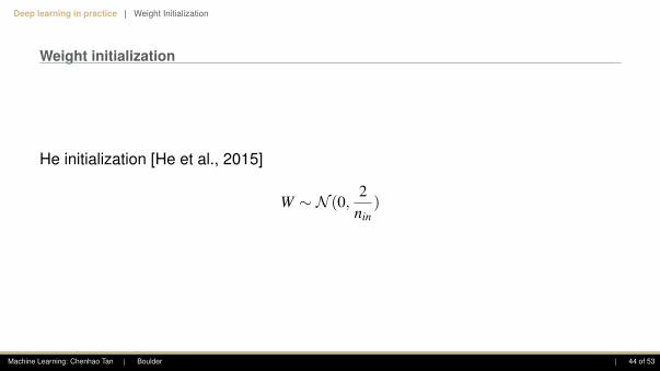
He initialization [He et al., 2015]
W ∼ N (0,2
nin)
Machine Learning: Chenhao Tan | Boulder | 44 of 53

Deep learning in practice | Weight Initialization
Weight initialization
This is an actively research area and next great idea may come from you!
Machine Learning: Chenhao Tan | Boulder | 45 of 53

Deep learning in practice | Model Architecture
Outline
History lesson
Deep learning in practiceImprove stochastic gradient descentUnstable gradientsData preprocessingWeight InitializationModel Architecture
Machine Learning: Chenhao Tan | Boulder | 46 of 53

Deep learning in practice | Model Architecture
ResNet
How to train a neural network with 100 layers? [He et al., 2016]
Machine Learning: Chenhao Tan | Boulder | 47 of 53

Deep learning in practice | Model Architecture
ResNet
Why is it hard to train a large number of layers?
Machine Learning: Chenhao Tan | Boulder | 48 of 53

Deep learning in practice | Model Architecture
ResNet
Simple solution:
Machine Learning: Chenhao Tan | Boulder | 49 of 53

Deep learning in practice | Model Architecture
ResNet
Machine Learning: Chenhao Tan | Boulder | 50 of 53

Deep learning in practice | Model Architecture
ResNet
Machine Learning: Chenhao Tan | Boulder | 51 of 53

Deep learning in practice | Model Architecture
References (1)
John Duchi, Elad Hazan, and Yoram Singer. Adaptive Subgradient Methods for Online Learning and StochasticOptimization. J. Mach. Learn. Res., 12:2121–2159, 2011. URLhttp://dl.acm.org/citation.cfm?id=1953048.2021068.
Xavier Glorot and Yoshua Bengio. Understanding the difficulty of training deep feedforward neural networks. InYee Whye Teh and Mike Titterington, editors, Proceedings of the Thirteenth International Conference onArtificial Intelligence and Statistics, volume 9 of Proceedings of Machine Learning Research, pages 249–256,Chia Laguna Resort, Sardinia, Italy, 13–15 May 2010. PMLR. URLhttp://proceedings.mlr.press/v9/glorot10a.html.
Kaiming He, Xiangyu Zhang, Shaoqing Ren, and Jian Sun. Delving deep into rectifiers: Surpassing human-levelperformance on imagenet classification. In The IEEE International Conference on Computer Vision (ICCV),December 2015.
Kaiming He, Xiangyu Zhang, Shaoqing Ren, and Jian Sun. Deep residual learning for image recognition. InProceedings of the IEEE Conference on Computer Vision and Pattern Recognition, 2016.
Sergey Ioffe and Christian Szegedy. Batch normalization: Accelerating deep network training by reducing internalcovariate shift. In Francis Bach and David Blei, editors, Proceedings of the 32nd International Conference onMachine Learning, volume 37 of Proceedings of Machine Learning Research, pages 448–456, Lille, France,07–09 Jul 2015. PMLR. URL http://proceedings.mlr.press/v37/ioffe15.html.
Machine Learning: Chenhao Tan | Boulder | 52 of 53

Deep learning in practice | Model Architecture
References (2)
Diederik P Kingma and Jimmy Ba. Adam: A Method for Stochastic Optimization. In Proceedings of ICLR, 2014.
Alex Krizhevsky, Ilya Sutskever, and Geoffrey E Hinton. ImageNet Classification with Deep Convolutional NeuralNetworks. In Proceedings of the 25th International Conference on Neural Information Processing Systems,2012.
Nitish Srivastava, Geoffrey Hinton, Alex Krizhevsky, Ilya Sutskever, and Ruslan Salakhutdinov. Dropout: A simpleway to prevent neural networks from overfitting. Journal of Machine Learning Research, 15:1929–1958, 2014.URL http://jmlr.org/papers/v15/srivastava14a.html.
Machine Learning: Chenhao Tan | Boulder | 53 of 53


![faculty.gordon.edufaculty.gordon.edu/hu/bi/...Videos/...Lecture05_Gen1_1_Questions.docx · Web view[5B] A.In the beginning was the word and the word was with God *B.In the beginning](https://img.pdfslide.us/doc/110x75/5cada79288c993220b8e0da0/-web-view5b-ain-the-beginning-was-the-word-and-the-word-was-with-god-bin.jpg)