MACHINE LEARNING-BASED OBJECT TRACKING · 2020-05-02 · APPENDIX 1 – MATLAB code for object tracking using HOG, PCA and SVM ... Implementation of the two techniques are done in

MACHINE LEARNING-BASEDOBJECT TRACKING

Rajasekhar NannapaneniSr Principal Engineer, Solutions ArchitectDell [email protected]

Knowledge Sharing Article © 2019 Dell Inc. or its subsidiaries.

2019 Dell Technologies Proven Professional Knowledge Sharing 2

Table of Contents

Abstract ...................................................................................................................................................... 3

A1.1 Introduction ....................................................................................................................................... 4

A1.2 Feature extraction techniques: .......................................................................................................... 4

A1.2.1 Histogram of Gradients ................................................................................................................... 5

A1.2.2 Principal Component Analysis ........................................................................................................ 5

A1.3 Classification techniques ................................................................................................................... 7

A1.3.1 Naïve Bayes ..................................................................................................................................... 7

A1.3.2 Support Vector Machine ................................................................................................................. 7

B2.1 Loading the video and division into frames ....................................................................................... 9

B2.2 Implementation of feature extraction - HOG .................................................................................. 11

B2.3 Implementation of feature reduction - PCA .................................................................................... 12

B2.4 Implementation of classification techniques SVM and Naïve Bayes ............................................... 13

B2.5 Measure to evaluate Object tracking .............................................................................................. 16

B2.6 Performance evaluation of the Classifiers ....................................................................................... 19

References................................................................................................................................................ 20

APPENDIX 1 – MATLAB code for object tracking using HOG, PCA and SVM ........................................... 21

APPENDIX 2– MATLAB code for object tracking using HOG, PCA and Naïve Bayes ................................ 25

Glossary

GMM Gaussian Mixture Models HOG Histogram of Oriented Gradients MCMC Markov Chain Monte Carlo MSE Mean Square Error PCA Principal Component Analysis RGB RED GREEN BLUE SVM Support Vector Machines

Disclaimer: The views, processes or methodologies published in this article are those of the author. They do

not necessarily reflect Dell Technologies’ views, processes or methodologies.


Abstract

Object tracking – a complex challenge in the domain of computer vision – tracks a specific object such as a

person, car or any other moving object in a video stream of underlying images.

Object tracking becomes useful in vehicle parking and security-based applications such as surveillance,

astronomy, and so on. Once an object is locked in a given image, the object tracking model is trained with

the features of that specific object, i.e. shape, color, size, presence, and position. This trained model can be

used to track this specific object in a stream of images.

The complexities involved in object tracking could be due to occlusions in the images, abrupt changes in

behavior of the object, i.e. speed, shape, motion of the camera, and such.

Several approaches exist today for tracking the object and in this article a new machine learning algorithm

is developed which aims to achieve higher accuracies for object tracking.


A1.1 Introduction

Object tracking is one of several applications leveraging the benefits of artificial intelligence (AI). In simple

terms, object tracking tracks an object of interest.

Examples include tracking a person via a video surveillance camera for security reasons, tracking an

unidentified flying object in the sky, tracking a planet or a comet in night sky from the captured frames of a

telescope, tracking a parked vehicle in a huge parking lot, etc.

Video captured from the cameras act as input to the object tracking system and various object tracking

methods exists. Deep learning (DL) is becoming popular in object tracking-based applications; however, it

requires significant processing power and may not be practical for simple or small-scale applications.

In this article, classical machine learning techniques such as PCA, HOG, SVM and Naïve Bayes are used to

perform object tracking which do not require compute to the extent that deep learning does and still

perform reasonably well for object tracking.

This article details two methods for object tracking – 1) HOG + PCA+ SVM 2) HOG + PCA + Naïve Bayes.

Part A of this article gives an overview of each of the feature extraction techniques such as HOG and PCA,

detailing the mechanism in which these techniques extract features from a given dataset.

Part B of this article provides design and implementation of object tracking for a benchmark dataset known

as dragon baby dataset. The test results were captured and a comparison of the two techniques is made

based on the performance of the algorithms.

Implementation of the two techniques are done in MATLAB and the code is mentioned in the APPENDIX.

A1.2 Feature extraction techniques

Various feature extraction techniques exist of which two – PCA and HOG – are used in this article that could

extract the relevant features and descriptions of the image frames in the video.

Though these two techniques are described as feature extractor’s, the actual description could be that the

HOG is a feature descriptor while PCA reduces the dimensionality of the features or, in other words, maps

the features to a different representation to facilitate classifier algorithm.


A1.2.1 Histogram of Gradients

A well-known approach in the field of computer vision, Histogram of Gradients (HOG) can provide feature

descriptions for any given image.

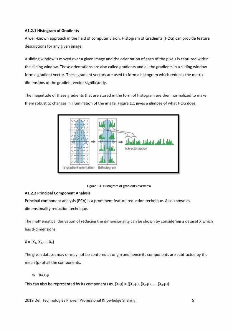
A sliding window is moved over a given image and the orientation of each of the pixels is captured within

the sliding window. These orientations are also called gradients and all the gradients in a sliding window

form a gradient vector. These gradient vectors are used to form a histogram which reduces the matrix

dimensions of the gradient vector significantly.

The magnitude of these gradients that are stored in the form of histogram are then normalized to make

them robust to changes in illumination of the image. Figure 1.1 gives a glimpse of what HOG does.

Figure 1.1: Histogram of gradients overview

A1.2.2 Principal Component Analysis

Principal component analysis (PCA) is a prominent feature reduction technique. Also known as

dimensionality reduction technique.

The mathematical derivation of reducing the dimensionality can be shown by considering a dataset X which

has d-dimensions.

X = {X1, X2, …. Xd}

The given dataset may or may not be centered at origin and hence its components are subtracted by the

mean (µ) of all the components.

X=X-µ

This can also be represented by its components as, (X-µ) = {(X1-µ), (X2-µ), …. (Xd-µ)}


The given dataset X has to be projected on to new dimensions e which in turn gives new coordinates,

X’ = (X-µ)Tej

X’ =

[ (𝑋 − µ)𝑒1

(𝑋 − µ)𝑒2

.

.(𝑋 − µ)𝑒𝑚]

=

[

(𝑋1 − 𝜇1)𝑒11 + (𝑋2 − 𝜇2)𝑒12 + . . . . . + (𝑋𝑑 − 𝜇𝑑)𝑒1𝑑

(𝑋1 − 𝜇1)𝑒21 + (𝑋2 − 𝜇2)𝑒22 + . . . . . + (𝑋𝑑 − 𝜇𝑑)𝑒2𝑑

.

.

.(𝑋1 − 𝜇1)𝑒𝑚1 + (𝑋2 − 𝜇2)𝑒𝑚2 + . . . . . + (𝑋𝑑 − 𝜇𝑑)𝑒𝑚𝑑]

The variance of the projection (V) = 1

𝑛 Σ [𝑋′ − 𝜇]2 =

1

𝑛 Σ [Σ (𝑋𝑒) − 𝜇]2

The constraints of e are of unit length and hence Lagrange multiplier (𝜆) is introduced,

V = 1

𝑛 Σ [Σ (𝑋𝑒)]2 − 𝜆 [(Σ 𝑒)2 − 1]

The eigen vectors are in the director of maximum variance and hence its essential to find the maximum.

𝜕𝑉

𝜕𝑒=

2

𝑛 Σ (Σ𝑥𝑒)𝑥 − 2𝜆𝑒 = 0

Σ 𝑒 = 𝜆 𝑒 ; where 𝜆 is the eigen value

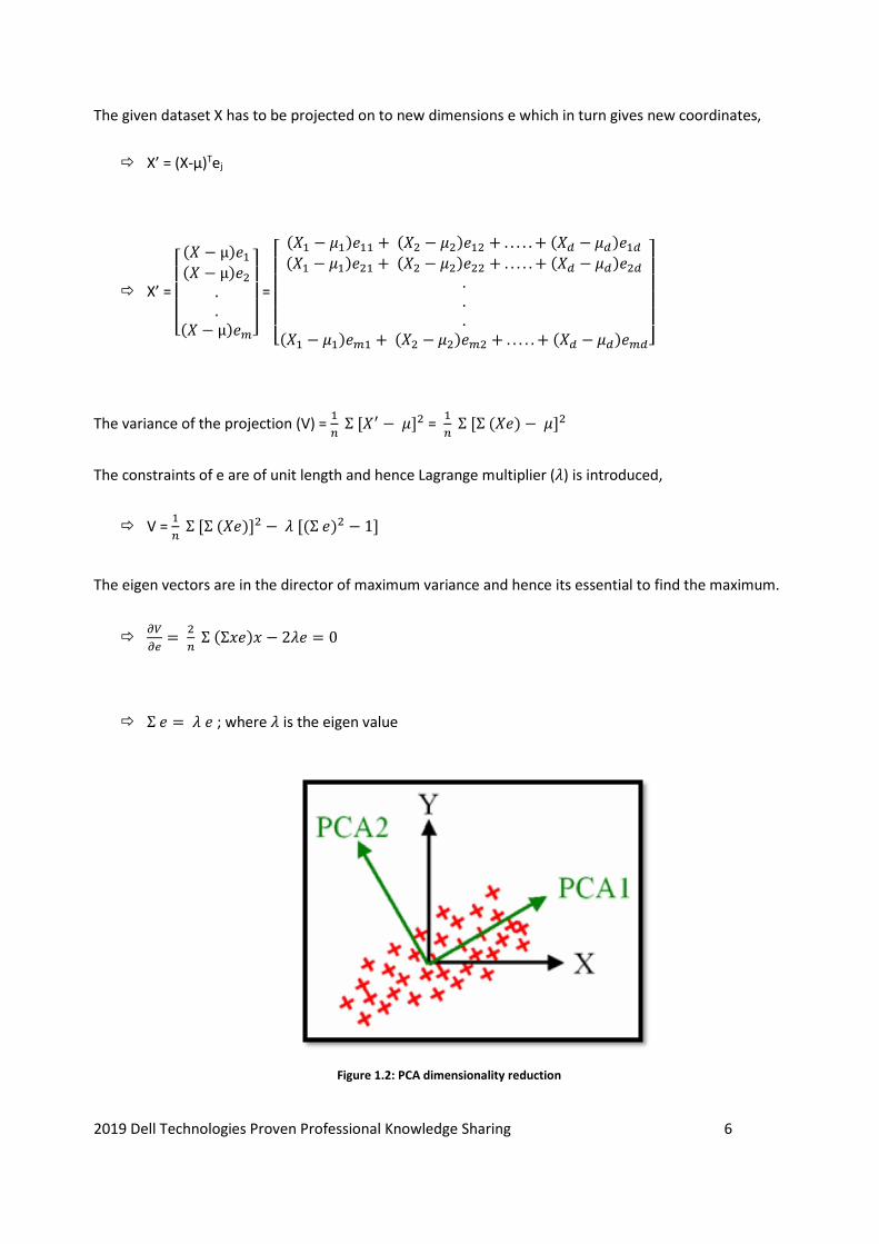
Figure 1.2: PCA dimensionality reduction


Principal components are nothing but the eigen vectors in the new dimension e. Hence for a given dataset

X, the principal components can be found by first projecting the vectors to a new dimension and then

finding the eigen vectors of the new dimensional data. The number of eigen vectors is equal to the number

of principal components as shown in Figure 1.2.

A1.3 Classification techniques

Several classification techniques exist of which two of the techniques – SVM and Naïve Bayes – are used in

this article that could classify the features extracted from the video frames.

SVM is generally more suitable in combination with HOG feature descriptor but in this article, we will also

use Naïve Bayes as a classification technique to compare the outcomes.

A1.3.1 Naïve Bayes

Naïve Bayes is one of the oldest classification techniques that uses Bayes theorem from probability theory

for performing classification.

According to Bayes theorem, 𝑃(𝐴/𝐵) = 𝑃(𝐴 ∩𝐵)

𝑃(𝐵) =

𝑃(𝐵/𝐴)∗𝑃(𝐴)

𝑃(𝐵) ; where P(B) = ∑𝑃(𝐵/𝐴) ∗ 𝑃(𝐴)

The Bayes theorem represents, Posterior = 𝐿𝑖𝑘𝑒𝑙𝑖ℎ𝑜𝑜𝑑∗𝑃𝑟𝑖𝑜𝑟

𝐸𝑣𝑖𝑑𝑒𝑛𝑐𝑒

If we consider 𝜔1 and 𝜔2 are two classes and x is a dependent vector then as per Bayes theorem,

𝑃(𝜔𝑖/𝑥) =𝑃(𝑥/𝜔𝑖)∗𝑃(𝜔𝑖)

𝑃(𝑥) ; where 𝑃(𝑥) = ∑𝑃(𝑥/𝜔𝑖) ∗ 𝑃(𝜔𝑖) and 𝜔𝑖 can be 𝜔1 or 𝜔2.

For a given x, if 𝑃(𝜔1/𝑥) > 𝑃(𝜔2/𝑥); then class 𝜔1 is decided else class 𝜔2 is decided. This case of 2 class

classification can be easily extended to multiple classes.

A1.3.2 Support Vector Machine

Support vector machines (SVM) is a classifier that is non-probabilistic in nature and the classification

happens through a hyperplane. The simplest form of SVM is a linear SVM whose hyperplane is linear and

the other could be the nonlinear SVM which uses a kernel trick to perform the classification.

Let’s consider a 2-class SVM classifier where the aim is to separate the data using a higher dimensional

hyperplane (𝜔. 𝑥 + 𝑏 = 0).


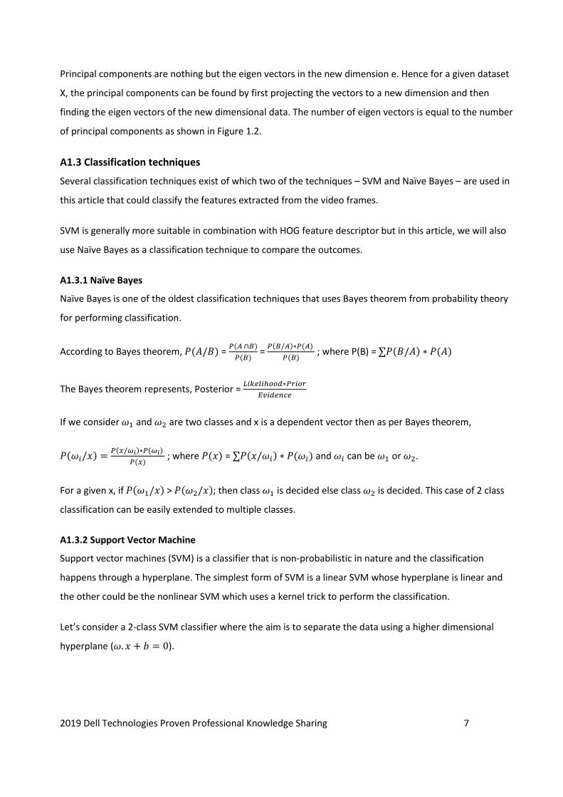
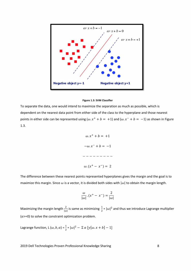
Figure 1.3: SVM Classifier

To separate the data, one would intend to maximize the separation as much as possible, which is

dependent on the nearest data point from either side of the class to the hyperplane and those nearest

points in either side can be represented using (𝜔. 𝑥+ + 𝑏 = +1) and (𝜔. 𝑥− + 𝑏 = −1) as shown in Figure

1.3.

𝜔. 𝑥+ + 𝑏 = +1

−𝜔. 𝑥− + 𝑏 = −1

− − − − − − − − −

𝜔. (𝑥+ − 𝑥−) = 2

The difference between these nearest points represented hyperplanes gives the margin and the goal is to

maximize this margin. Since 𝜔 is a vector, it is divided both sides with |𝜔| to obtain the margin length.

𝜔

|𝜔|. (𝑥+ − 𝑥−) =

2

|𝜔|

Maximizing the margin length 2

|𝜔| is same as minimizing

1

2∗ |𝜔|2 and thus we introduce Lagrange multiplier

(𝛼>=0) to solve the constraint optimization problem.

Lagrange function, L (𝜔, 𝑏, 𝛼) = 1

2∗ |𝜔|2 − Σ 𝛼 [𝑦[𝜔. 𝑥 + 𝑏] − 1]


Minimizing the Lagrange function L, 𝜕𝐿

𝜕𝑏= Σ 𝛼. 𝑦 = 0 and

𝜕𝐿

𝜕𝜔= Σ 𝛼. 𝑦. 𝑥 = 0

𝑦 = 𝑓(𝑥) = Σ 𝛼. 𝑦. 𝑥𝑇 . 𝑥 + 𝑏 , which is the decision boundary or the hyperplane that classifies the

data.

The term 𝑥𝑇 . 𝑥 indicates the dot product and means that it’s a projection of one vector over another which

means it is computing similarity of the data points:

1) If 𝑥𝑇 . 𝑥 are perpendicular, then dot product is 0.

2) If 𝑥𝑇 . 𝑥 are in same direction, it implies large +ve value indicating that they are on +ve side of the

hyperplane.

3) If 𝑥𝑇 . 𝑥 are in same direction, it implies large -ve value indicating that they are on -ve side of the

hyperplane.

This classification is based on the linearly separable data else one needs to use kernel trick to classify the

data which is a nonlinear SVM.

B2.1 Loading the video and division into frames

The video frame dataset called dragon baby dataset was taken with 20 video frames of which 10 video

frames are used as training dataset and 10 of the video frames are used as testing dataset.

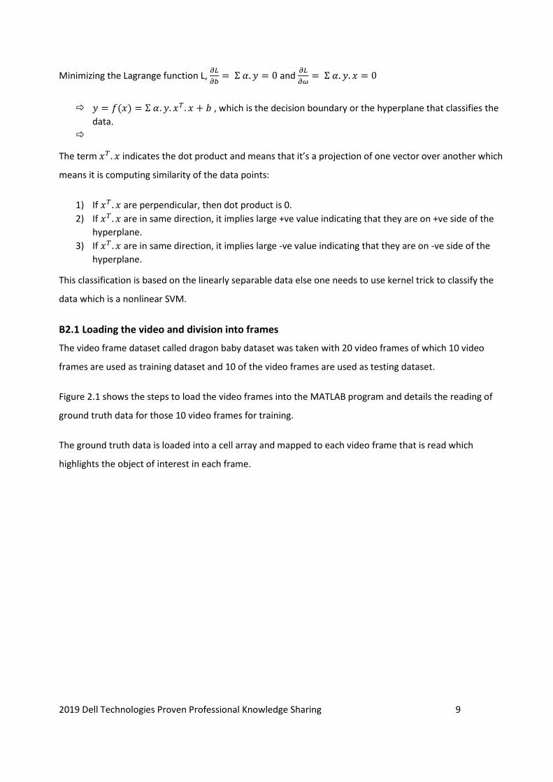
Figure 2.1 shows the steps to load the video frames into the MATLAB program and details the reading of

ground truth data for those 10 video frames for training.

The ground truth data is loaded into a cell array and mapped to each video frame that is read which

highlights the object of interest in each frame.


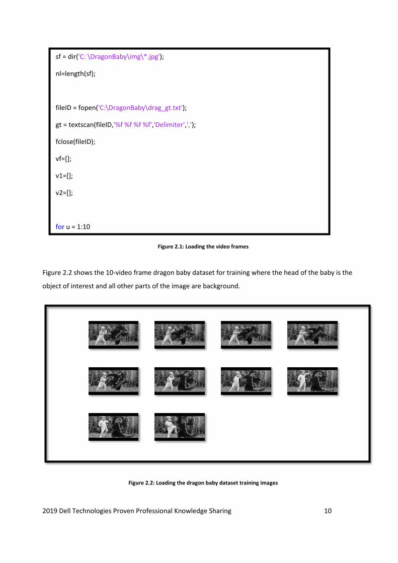
Figure 2.2 shows the 10-video frame dragon baby dataset for training where the head of the baby is the

object of interest and all other parts of the image are background.

sf = dir('C: \DragonBaby\img\*.jpg');

nl=length(sf);

fileID = fopen('C:\DragonBaby\drag_gt.txt');

gt = textscan(fileID,'%f %f %f %f','Delimiter',',');

fclose(fileID);

vf=[];

v1=[];

v2=[];

for u = 1:10

filename = strcat('C:\DragonBaby\img\',sf(u).name);

im= double(rgb2gray(imread(filename)));

x1=gt{1,1}(u);

y1=gt{1,2}(u);

w1=gt{1,3}(u);

h1=gt{1,4}(u);

face = imcrop(im,[x1,y1,w1,h1]);

end

Figure 2.1: Loading the video frames

Figure 2.2: Loading the dragon baby dataset training images


B2.2 Implementation of feature extraction - HOG

The MATLAB implementation of histogram of oriented gradients technique is mentioned in APPENDIX 1

and 2.

The training dataset consisting of 10-video frames is considered along with its corresponding ground truth

that highlights the baby’s head or in other words, the object of interest and any other part of the frame is

considered as background.

Each video frame image is cropped in according to the ground truth so that the features of the object of

interest can be extracted using histogram of oriented gradients technique. Similarly, the features of

background of the image is also extracted and labelled appropriately.

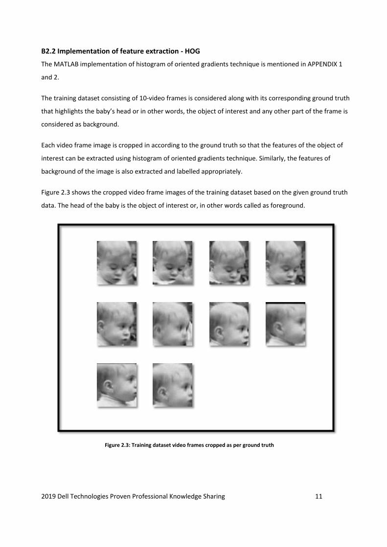
Figure 2.3 shows the cropped video frame images of the training dataset based on the given ground truth

data. The head of the baby is the object of interest or, in other words called as foreground.

Figure 2.3: Training dataset video frames cropped as per ground truth


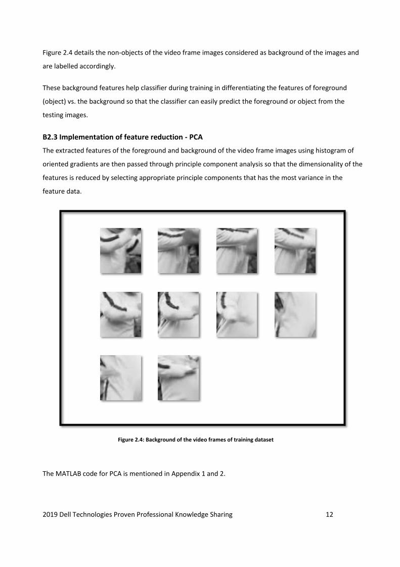
Figure 2.4 details the non-objects of the video frame images considered as background of the images and

are labelled accordingly.

These background features help classifier during training in differentiating the features of foreground

(object) vs. the background so that the classifier can easily predict the foreground or object from the

testing images.

B2.3 Implementation of feature reduction - PCA

The extracted features of the foreground and background of the video frame images using histogram of

oriented gradients are then passed through principle component analysis so that the dimensionality of the

features is reduced by selecting appropriate principle components that has the most variance in the

feature data.

The MATLAB code for PCA is mentioned in Appendix 1 and 2.

Figure 2.4: Background of the video frames of training dataset


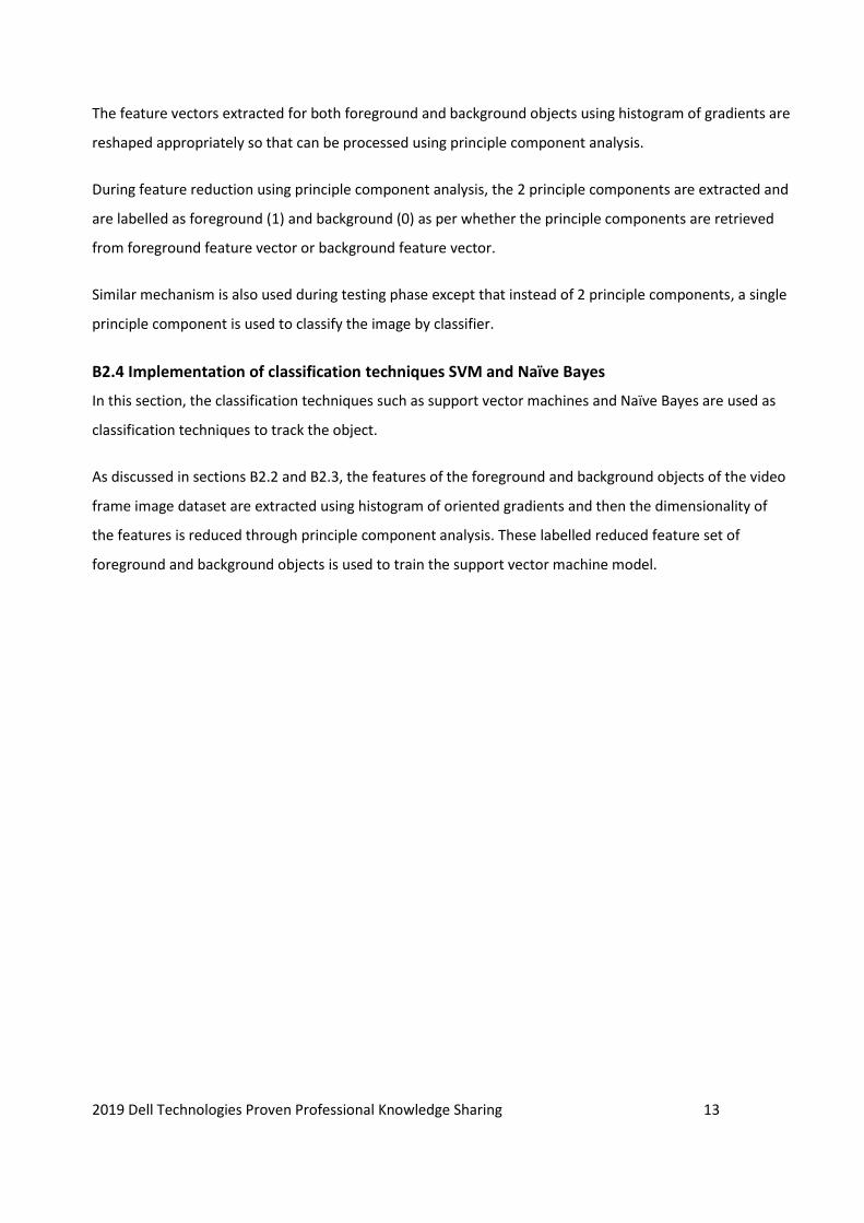
The feature vectors extracted for both foreground and background objects using histogram of gradients are

reshaped appropriately so that can be processed using principle component analysis.

During feature reduction using principle component analysis, the 2 principle components are extracted and

are labelled as foreground (1) and background (0) as per whether the principle components are retrieved

from foreground feature vector or background feature vector.

Similar mechanism is also used during testing phase except that instead of 2 principle components, a single

principle component is used to classify the image by classifier.

B2.4 Implementation of classification techniques SVM and Naïve Bayes

In this section, the classification techniques such as support vector machines and Naïve Bayes are used as

classification techniques to track the object.

As discussed in sections B2.2 and B2.3, the features of the foreground and background objects of the video

frame image dataset are extracted using histogram of oriented gradients and then the dimensionality of

the features is reduced through principle component analysis. These labelled reduced feature set of

foreground and background objects is used to train the support vector machine model.


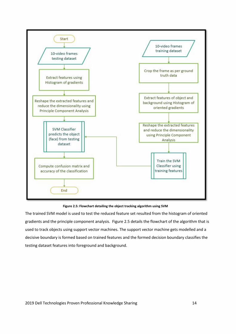
The trained SVM model is used to test the reduced feature set resulted from the histogram of oriented

gradients and the principle component analysis. Figure 2.5 details the flowchart of the algorithm that is

used to track objects using support vector machines. The support vector machine gets modelled and a

decisive boundary is formed based on trained features and the formed decision boundary classifies the

testing dataset features into foreground and background.

Figure 2.5: Flowchart detailing the object tracking algorithm using SVM


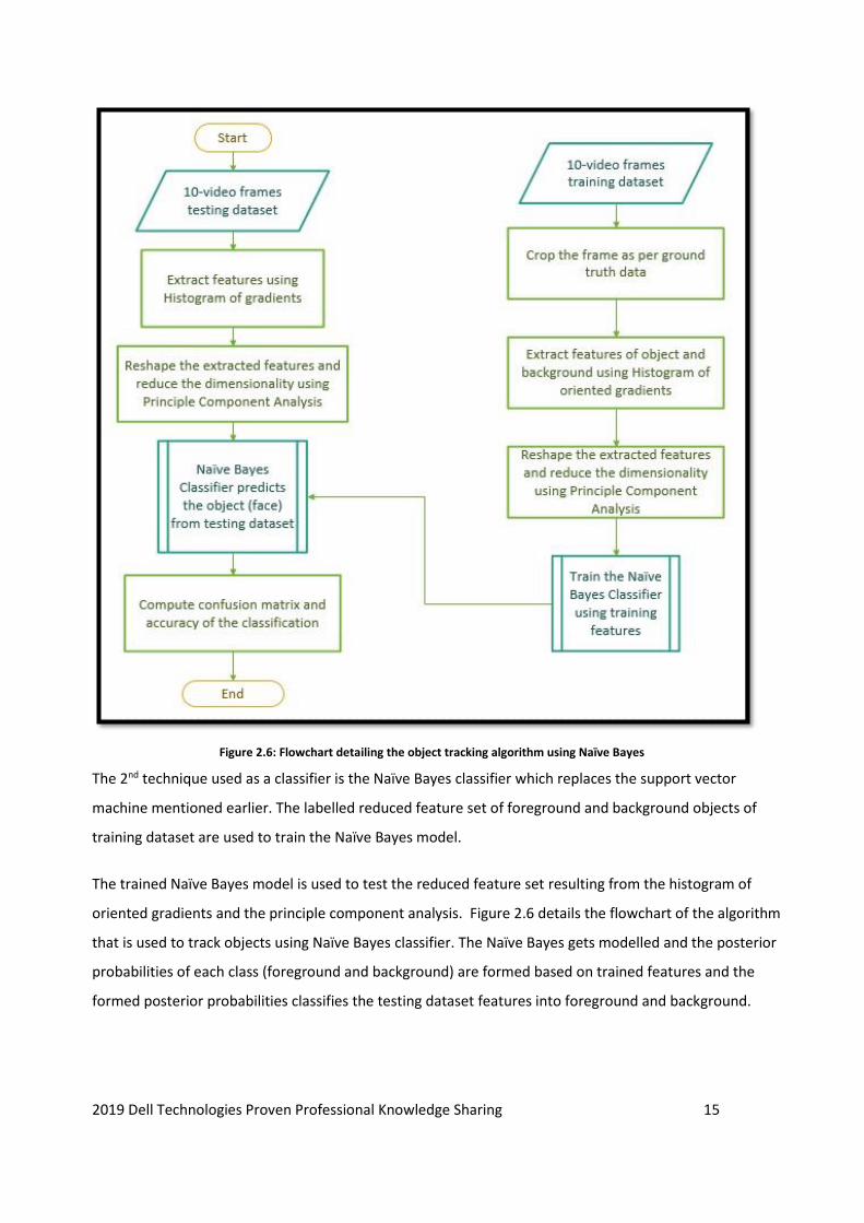
The 2nd technique used as a classifier is the Naïve Bayes classifier which replaces the support vector

machine mentioned earlier. The labelled reduced feature set of foreground and background objects of

training dataset are used to train the Naïve Bayes model.

The trained Naïve Bayes model is used to test the reduced feature set resulting from the histogram of

oriented gradients and the principle component analysis. Figure 2.6 details the flowchart of the algorithm

that is used to track objects using Naïve Bayes classifier. The Naïve Bayes gets modelled and the posterior

probabilities of each class (foreground and background) are formed based on trained features and the

formed posterior probabilities classifies the testing dataset features into foreground and background.

Figure 2.6: Flowchart detailing the object tracking algorithm using Naïve Bayes


The MATLAB code of SVM classification technique is mentioned in APPENDIX 1 and the MATLAB code of

Naïve Bayes classification technique is mentioned in APPENDIX 2.

B2.5 Measure to evaluate Object tracking

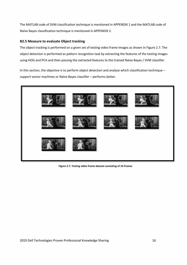
The object tracking is performed on a given set of testing video frame images as shown in Figure 2.7. The

object detection is performed as pattern recognition task by extracting the features of the testing images

using HOG and PCA and then passing the extracted features to the trained Naïve Bayes / SVM classifier.

In this section, the objective is to perform object detection and analyze which classification technique –

support vector machines or Naïve Bayes classifier – performs better.

Figure 2.7: Testing video frame dataset consisting of 10-frames


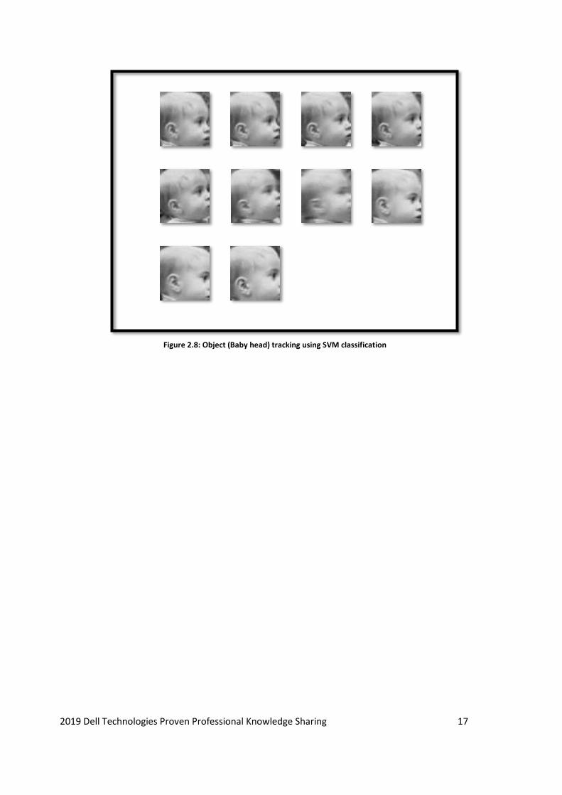
Figure 2.8: Object (Baby head) tracking using SVM classification


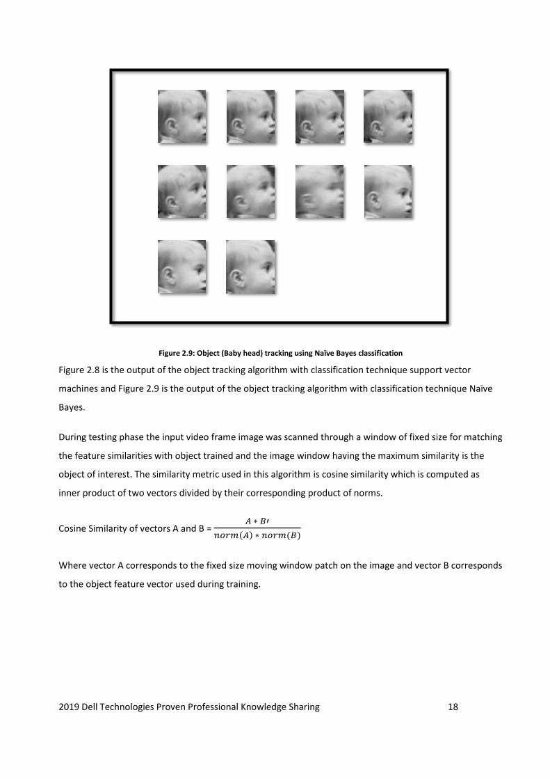
Figure 2.8 is the output of the object tracking algorithm with classification technique support vector

machines and Figure 2.9 is the output of the object tracking algorithm with classification technique Naïve

Bayes.

During testing phase the input video frame image was scanned through a window of fixed size for matching

the feature similarities with object trained and the image window having the maximum similarity is the

object of interest. The similarity metric used in this algorithm is cosine similarity which is computed as

inner product of two vectors divided by their corresponding product of norms.

Cosine Similarity of vectors A and B = 𝐴 ∗ 𝐵′

𝑛𝑜𝑟𝑚(𝐴) ∗ 𝑛𝑜𝑟𝑚(𝐵)

Where vector A corresponds to the fixed size moving window patch on the image and vector B corresponds

to the object feature vector used during training.

Figure 2.9: Object (Baby head) tracking using Naïve Bayes classification


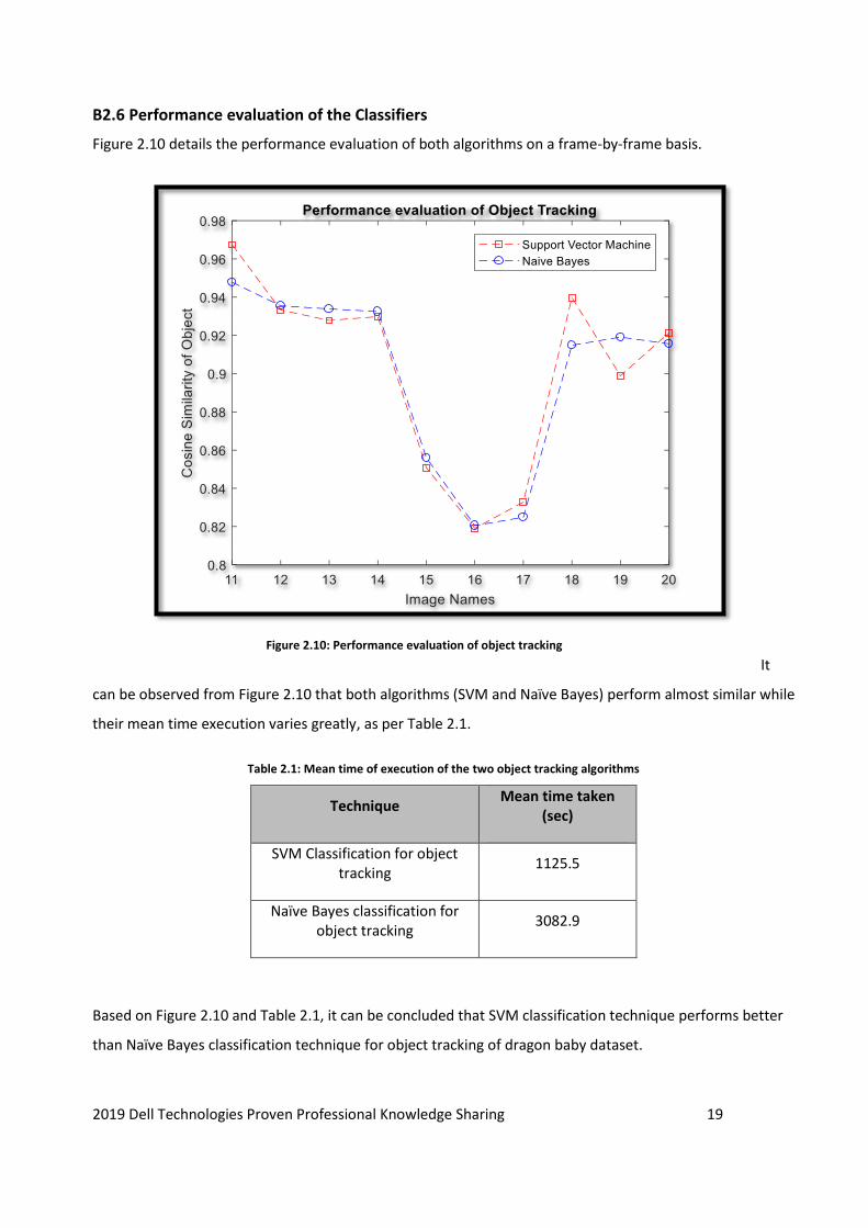
B2.6 Performance evaluation of the Classifiers

Figure 2.10 details the performance evaluation of both algorithms on a frame-by-frame basis.

It

can be observed from Figure 2.10 that both algorithms (SVM and Naïve Bayes) perform almost similar while

their mean time execution varies greatly, as per Table 2.1.

Table 2.1: Mean time of execution of the two object tracking algorithms

Technique Mean time taken

(sec)

SVM Classification for object tracking

1125.5

Naïve Bayes classification for object tracking

3082.9

Based on Figure 2.10 and Table 2.1, it can be concluded that SVM classification technique performs better

than Naïve Bayes classification technique for object tracking of dragon baby dataset.

Figure 2.10: Performance evaluation of object tracking


References

“[1] Christopher, M.B., 2016. PATTERN RECOGNITION AND MACHINE LEARNING. Springer-Verlag New

York.”

“[2] El Maroufy, H., Zyad, A. and Ziad, T., 2017. Bayesian Estimation of Multivariate Autoregressive Hidden

Markov Model with Application to Breast Cancer Biomarker Modeling. In Bayesian Inference. InTech.”

“[3] Geetha, M.P. and Subha, M.M., 2015. BREAST CANCER ANALYSIS IN MEDICAL MINING BASED ON

MARKOV CHAIN MONTE CARLO EXPECTATION MAXIMIZATION.”

“[4] Kowal, Marek & Filipczuk, Paweł & Obuchowicz, Andrzej & Korbicz, Józef. (2011). Computer-aided

diagnosis of breast cancer using Gaussian mixture cytological image segmentation. Journal of Medical

Informatics & Technologies. Vol. 17. 257-262.”

“[5] Martins, L.D.O., dos Santos, A.M., Silva, A.C. and Paiva, A.C., 2006, October. Classification of normal,

benign and malignant tissues using co-occurrence matrix and Bayesian neural network in mammographic

images. In Neural Networks, 2006. SBRN'06. Ninth Brazilian Symposium on (pp. 24-29). IEEE.”

“[6] Ogunsakin, R.E. and Siaka, L., 2017. Bayesian Inference on Malignant Breast Cancer in Nigeria: A

Diagnosis of MCMC Convergence. Asian Pacific Journal of Cancer Prevention, 18(10), pp.2709-2716.”

“[7] Scherrer, B., 2007. Gaussian mixture model classifiers. Lecture Notes, February.”

“[8] Sujith, & Jyothiprakash (2014). Pedestrian Detection-A Comparative Study Using HOG and COHOG.”


Appendix

Appendix 1 – MATLAB code for object tracking using HOG, PCA and SVM

clc;

clear;

close all;

tic;

sf = dir('C:\Users\dell\Documents\DragonBaby\DragonBaby\img\*.jpg');

nl=length(sf);

fileID = fopen('C:\Users\dell\Documents\DragonBaby\DragonBaby\drag_gt.txt');


fclose(fileID);

vf=[];

v1=[];

v2=[];

for u = 1:10

filename = strcat('C:\Users\dell\Documents\DragonBaby\DragonBaby\img\',sf(u).name);


x1=gt{1,1}(u);

y1=gt{1,2}(u);

w1=gt{1,3}(u);

h1=gt{1,4}(u);


[featureVector1,hogVisualization] = extractHOGFeatures(face);

bkgrd = imcrop(im,[160,140,w1,h1]);

[featureVector2,hogVisualization] = extractHOGFeatures(bkgrd);


[r,c]=size(featureVector1);

%v1=[v1;featureVector1];


fv1=reshape(featureVector1,[8,c/8]);


[Train_coeff1] = pca(fv1);


v1=[v1,Train_coeff1(:,1:2)];


vf=horzcat(v1,v2);

trainf=vf';

figure(1);

subplot (3,4,u);

imshow(uint8(im));

figure(2);

subplot (3,4,u);

imshow(uint8(face));

figure(3);

subplot (3,4,u);

imshow(uint8(bkgrd));

end


group=[1;1;0;0;1;1;0;0;1;1;0;0;1;1;0;0;1;1;0;0;1;1;0;0;1;1;0;0;1;1;0;0;1;1;0;0;1;1;0;0];

SVMModel = fitcsvm(trainf,group);

k=1;

for i1 = 11:20

filename = strcat('C:\Users\dell\Documents\DragonBaby\DragonBaby\img\',sf(i1).name);

im1= double(rgb2gray(imread(filename)));

[m n]=size(im1);

fv=0;

csf=0;

for i=20:m-h1

for j=100:n-(6*w1)

it=im1(i:i+h1,j:j+w1);

[featureVector3,hogVisualization] = extractHOGFeatures(it);

fv=fv+1;


[Test_coeff3] = pca(fv3);

tc=Test_coeff3(:,1:1);

tc=tc';

ans = predict(SVMModel,tc);

if ans==1

cs=((featureVector3*featureVector1')/(norm(featureVector3)*norm(featureVector1)))';

if cs > csf

csf=cs;

xf=j;

yf=i;

end


end

end

end

imf=imcrop(im1,[xf,yf,w1,h1]);

figure(4);

subplot(3,4,k);

imshow(uint8(im1));

figure(5);

subplot(3,4,k);

imshow(uint8(imf));

similarity(k)=csf;

k=k+1;

end

figure(6);

plot(1:10,similarity,'--b*');

xlabel ('Image Names');

ylabel ('Cosine Similarity with object (Face)');

title('Performance evaluation of Object tracking');

ti=toc


Appendix 2– MATLAB code for object tracking using HOG, PCA and Naïve Bayes

clc;

clear;

close all;

tic;

sf = dir('C:\Users\dell\Documents\DragonBaby\DragonBaby\img\*.jpg');

nl=length(sf);

fileID = fopen('C:\Users\dell\Documents\DragonBaby\DragonBaby\drag_gt.txt');


fclose(fileID);

vf=[];

v1=[];

v2=[];

for u = 1:10

filename = strcat('C:\Users\dell\Documents\DragonBaby\DragonBaby\img\',sf(u).name);


x1=gt{1,1}(u);

y1=gt{1,2}(u);

w1=gt{1,3}(u);

h1=gt{1,4}(u);


[featureVector1,hogVisualization] = extractHOGFeatures(face);

bkgrd = imcrop(im,[160,140,w1,h1]);

[featureVector2,hogVisualization] = extractHOGFeatures(bkgrd);


[r,c]=size(featureVector1);









vf=horzcat(v1,v2);

trainf=vf';

figure(1);

subplot (3,4,u);

imshow(uint8(im));

figure(2);

subplot (3,4,u);

imshow(uint8(face));

figure(3);

subplot (3,4,u);

imshow(uint8(bkgrd));


end

group=[1;1;0;0;1;1;0;0;1;1;0;0;1;1;0;0;1;1;0;0;1;1;0;0;1;1;0;0;1;1;0;0;1;1;0;0;1;1;0;0];

NB_Model = fitcnb(trainf,group);

k=1;

for i1 = 11:20

filename = strcat('C:\Users\dell\Documents\DragonBaby\DragonBaby\img\',sf(i1).name);

im1= double(rgb2gray(imread(filename)));

[m n]=size(im1);

fv=0;

csf=0;

for i=20:m-h1

for j=100:n-(6*w1)

it=im1(i:i+h1,j:j+w1);

[featureVector3,hogVisualization] = extractHOGFeatures(it);

fv=fv+1;


[Test_coeff3] = pca(fv3);

tc=Test_coeff3(:,1:1);

tc=tc';

ans = predict(NB_Model,tc);

if ans==1

cs=((featureVector3*featureVector1')/(norm(featureVector3)*norm(featureVector1)))';

if cs > csf

csf=cs;


xf=j;

yf=i;

end

end

end

end

imf=imcrop(im1,[xf,yf,w1,h1]);

figure(4);

subplot(3,4,k);

imshow(uint8(im1));

figure(5);

subplot(3,4,k);

imshow(uint8(imf));

similarity(k)=csf;

k=k+1;

end

figure(6);

plot(1:10,similarity,'--b*');

xlabel ('Image Names');

ylabel ('Cosine Similarity with object (Face)');

title('Performance evaluation of Object tracking');

ti=toc


Dell Technologies believes the information in this publication is accurate as of its publication date. The

information is subject to change without notice.

THE INFORMATION IN THIS PUBLICATION IS PROVIDED “AS IS.” DELL TECHNOLOGIES MAKES NO

RESPRESENTATIONS OR WARRANTIES OF ANY KIND WITH RESPECT TO THE INFORMATION IN THIS

PUBLICATION, AND SPECIFICALLY DISCLAIMS IMPLIED WARRANTIES OF MERCHANTABILITY OR FITNESS FOR

A PARTICULAR PURPOSE.

Use, copying and distribution of any Dell Technologies software described in this publication requires an

applicable software license.

Copyright © 2019 Dell Inc. or its subsidiaries. All Rights Reserved. Dell Technologies, Dell, EMC, Dell EMC

and other trademarks are trademarks of Dell Inc. or its subsidiaries. Other trademarks may be trademarks

of their respective owners.