Embed Size (px)
Citation preview

This thesis has been submitted in fulfilment of the requirements for a postgraduate degree
(e.g. PhD, MPhil, DClinPsychol) at the University of Edinburgh. Please note the following
terms and conditions of use:
This work is protected by copyright and other intellectual property rights, which are
retained by the thesis author, unless otherwise stated.
A copy can be downloaded for personal non-commercial research or study, without
prior permission or charge.
This thesis cannot be reproduced or quoted extensively from without first obtaining
permission in writing from the author.
The content must not be changed in any way or sold commercially in any format or
medium without the formal permission of the author.
When referring to this work, full bibliographic details including the author, title,
awarding institution and date of the thesis must be given.

Machine Learning and Privacy Preserving
Algorithms for Spatial and Temporal
Sensing
Abhirup Ghosh
TH
E
U N I V E RS
IT
Y
OF
ED I N B U
RG
H
Doctor of Philosophy
Laboratory for Foundations of Computer Science
School of Informatics
University of Edinburgh
2019

Abstract
Sensing physical and social environments are ubiquitous in modern mobile phones,
IoT devices, and infrastructure-based settings. Information engraved in such
data, especially the time and location attributes have unprecedented potential
to characterize individual and crowd behavior, natural and technological pro-
cesses. However, it is challenging to extract abstract knowledge from the data
due to its massive size, sequential structure, asynchronous operation, noisy char-
acteristics, privacy concerns, and real time analysis requirements. Therefore, the
primary goal of this thesis is to propose theoretically grounded and practically
useful algorithms to learn from location and time stamps in sensor data. The
proposed methods are inspired by tools from geometry, topology, and statistics.
They leverage structures in the temporal and spatial data by probabilistically
modeling noise, exploring topological structures embedded, and utilizing statisti-
cal structure to protect personal information and simultaneously learn aggregate
information. Proposed algorithms are geared towards streaming and distributed
operation for efficiency. The usefulness of the methods is argued using mathe-
matical analysis and empirical experiments on real and artificial datasets.
iii

Lay Summary
Modern personal devices continuously record the social and physical context
of their users. Time and location stamps associated with these sensing data are
often important for personalization and optimization across applications. How-
ever, it is challenging to learn high level abstract knowledge from the sensing
data mainly due to huge dataset size, noisy environment, and realtime analysis
requirement. Moreover, even anonymized data used with best of intentions can
leak sensitive information about data contributors. So, in this thesis, we discuss
novel mechanisms inspired by statistics and geometry to learn fundamental pat-
terns inscribed in the data while protecting the privacy of the individual users.
Following are the specific problems we address here.
Periodicity is fundamental and useful to characterize and forecast time series.
For example, our footsteps, heart beats, traffic surges, etc., have regular repeating
patterns. But, it is challenging to automatically detect the periodicity in real
world signals due to dynamic period and phase and therefore popular frequency
domain methods do not apply. Here, we propose an online algorithm that guesses
several periods and iteratively refines them as it observes the signal.
Timings of important events are often sensitive. For example, we don’t want
an adversary to know the exact check-in times, but the aggregate information is
required for service optimization. We propose techniques to introduce carefully
chosen noise such as perturb the event timings or introduce spurious events so that
no adversary can learn sensitive event timings with confidence, while aggregate
inferences, like event density is preserved.
Location is another fundamental attribute in the sensing data. Mobility traces
are important in many practical applications, for example, predicting future loca-
tion. We propose a general framework to apply standard machine learning tools
for location trajectories. The fundamental idea is that the way the objects move
around the obstacles in the domain constitutes the most important characteristics
of the mobility pattern.
Location is also sensitive, for example, check-in at a hospital. To protect
location privacy, we develop algorithms to protect exact location stamps while
ensuring that the aggregate inferences are useful. These mechanisms are well
beyond simple anonymization and are inspired by the strongest form of privacy.
v


Acknowledgements
First and foremost, I want to thank Rik, my primary supervisor. Our numer-
ous technical discussions have shaped all the works in this thesis and beyond. His
guidance, continuous encouragement, and support have taught me perseverance
and helped me to survive in the time of despair. His ability to make complex
arguments simple, find the core concepts with ease, and connect myriad ideas
had taught me essential skills of a researcher. I consider myself blessed to have
the chance to work with him. I also thank Mahesh, my second supervisor, for
showing me new directions regarding both specific research questions and setting
broad research agenda. From all the academics in the NetSys, especially, Rik,
Mahesh, and Paul, I learned the science and art of presentation.
I am fortunate to work with Christopher Lucas, Subramanian Ramamoorthy,
and Jie Gao. They all have contributed significantly to this thesis. I thank Chris
for his technical guidance in the work on periodicity, being my examiner in the
annual reviews, and continuously helping me to shape my research and career. I
thank Ram as his ideas helped us to structure our work on mobility analysis. I
am thankful to Jie for her support in all the privacy related works in this thesis.
Her vast experience, technical depth, and conceptual breadth essentially textured
these works. I am grateful to Paul Patras and Thomas Heinis for taking the time
to review my thesis and being the examiners in my defense.
I appreciate Jiaxin for our discussions regarding Chapter 3 and Chapter 5. I
feel lucky to work with brilliant colleagues and kind friends, Yota, Maria, and
Benedek. I specially thank Benedek for his contribution in the experiments re-
garding location prediction in Section 4.7. I thank Yota and Maria for numerous
technical discussions and continuous support in every way possible. I am also
thankful to Lauren for our discussions on privacy.
I am also grateful to have Rajkaran as a friend and a colleague. Our countless
technical and non-technical discussions helped me in research and life. I thank
Mah-Rukh for our discussions on network measurement. I also appreciate Manick,
Priyank, Saumay, Aprit, Rakesh, Prasun, and Sumit for their support to continue
life outside of research.
Last but not the least, without my family this thesis would not have been
possible. They continuously guided me to be a better human being and inspired
me to cross the hardest hurdles.
vii

I first appreciate my parents; Without them, I would not have come this far in
life. From the time I remember, they nurtured me to have all the qualities of life
that they could think of. Their patience, blessings, continuous encouragement,
and support had started weaving the very letters of this thesis long before I
started writing it. Their continuous struggle reminds me that life is much bigger
than a PhD and gave me the essential strength to overcome all the obstacles in
the way to this book.
Finally, I thank my loving wife, Maitri, for walking the whole journey with
me. A PhD is not a bed of roses neither it is full of nails. We walked the bloody
roads of desperation as well as the time of euphoria together. She deserves equal
credit for this thesis if not more. The hot meals that she prepared every single
day, sleepless nights that she spent to make my writing perfect or my presentation
flawless, responsibilities that she alone handled to run the family, vacations that
she organized take a necessary break from stressful life, countless prayers that
she made, sacrifices that she made with her life and career have all counted and
finally resulted in this book.
viii


To my loving family,
xi

Table of Contents
1 Introduction 1
1.1 Challenges in learning from sensor data . . . . . . . . . . . . . . . 2
1.2 Key topics in learning from sensor data . . . . . . . . . . . . . . . 3
1.2.1 Sensor data collection . . . . . . . . . . . . . . . . . . . . 4
1.2.2 Learning from location and time stamps . . . . . . . . . . 6
1.2.3 Preserving Privacy . . . . . . . . . . . . . . . . . . . . . . 8
1.3 Summary . . . . . . . . . . . . . . . . . . . . . . . . . . . . . . . 10
1.3.1 Learning From Temporal Streams . . . . . . . . . . . . . . 10
1.3.2 Learning From Spatial Data . . . . . . . . . . . . . . . . . 11
I Learning from Temporal Streams 15
2 Periodicity in Noisy Event Streams 17
2.1 Introduction . . . . . . . . . . . . . . . . . . . . . . . . . . . . . . 17
2.2 Related works . . . . . . . . . . . . . . . . . . . . . . . . . . . . . 20
2.3 Model and problem description . . . . . . . . . . . . . . . . . . . 21
2.4 Particle filter design . . . . . . . . . . . . . . . . . . . . . . . . . 24
2.4.1 Particle filters and importance sampling . . . . . . . . . . 24
2.4.2 Particle filter for discovering periodicity . . . . . . . . . . . 27
2.4.3 Practical optimizations for noisy environments . . . . . . . 30
2.5 Experimental evaluation . . . . . . . . . . . . . . . . . . . . . . . 31
2.5.1 Comparison algorithms . . . . . . . . . . . . . . . . . . . . 32
2.5.2 Sensitivity to noise and model parameters . . . . . . . . . 32
2.5.3 Experiments on real datasets . . . . . . . . . . . . . . . . 40
3 Private Sensing of Asynchronous Event Sequences 45
3.1 Introduction . . . . . . . . . . . . . . . . . . . . . . . . . . . . . . 45
xiii
3.2 Related Work . . . . . . . . . . . . . . . . . . . . . . . . . . . . . 48
3.3 Statistical Privacy and Challenges in Streaming Event Data . . . 50
3.3.1 Continuous Publication of Events . . . . . . . . . . . . . . 52
3.3.2 Pufferfish Privacy . . . . . . . . . . . . . . . . . . . . . . . 54
3.4 Model and problem statements . . . . . . . . . . . . . . . . . . . 55
3.4.1 Sensing Data Collection and Trust Relations . . . . . . . . 55
3.4.2 Utility: Range Queries . . . . . . . . . . . . . . . . . . . . 56
3.4.3 Adversary Model and Problem Statements . . . . . . . . . 56
3.5 Privacy mechanisms . . . . . . . . . . . . . . . . . . . . . . . . . 57
3.5.1 Problem 1: Protecting Event Times . . . . . . . . . . . . . 58
3.5.2 Problem 2: Protecting event existence in Poisson processes 59
3.5.3 Problem 3: Privacy of event order . . . . . . . . . . . . . . 61
3.6 Privacy service design and implementation . . . . . . . . . . . . . 61
3.6.1 System design as background Android service . . . . . . . 63
3.7 Experiments . . . . . . . . . . . . . . . . . . . . . . . . . . . . . . 63
3.7.1 Experimental Setup . . . . . . . . . . . . . . . . . . . . . . 64
3.7.2 Evaluating Event Time Privacy . . . . . . . . . . . . . . . 64
3.7.3 Evaluating Event Existance – Mechanism 2.1 . . . . . . . . 65
3.7.4 Comparison with existing methods. . . . . . . . . . . . . . 65
3.7.5 Time efficiency . . . . . . . . . . . . . . . . . . . . . . . . 65
3.8 Proofs of the Theorems . . . . . . . . . . . . . . . . . . . . . . . . 68
3.8.1 Proof of Theorem 1 . . . . . . . . . . . . . . . . . . . . . . 68
3.8.2 Proof of Theorem 2 . . . . . . . . . . . . . . . . . . . . . . 71
3.8.3 Proof of Theorem 4 . . . . . . . . . . . . . . . . . . . . . . 73
3.8.4 Proof of Theorem 5 . . . . . . . . . . . . . . . . . . . . . . 73
II Learning from Spatial Data 77
4 Topological Signatures For Fast Mobility Analysis 79
4.1 Introduction . . . . . . . . . . . . . . . . . . . . . . . . . . . . . . 80
4.2 Related work . . . . . . . . . . . . . . . . . . . . . . . . . . . . . 82
4.3 Theoretical background . . . . . . . . . . . . . . . . . . . . . . . . 83
4.3.1 Discrete differential 1-forms and co-chains . . . . . . . . . 85
4.4 Topological signatures . . . . . . . . . . . . . . . . . . . . . . . . 85
4.5 Algorithms . . . . . . . . . . . . . . . . . . . . . . . . . . . . . . . 87
xiv

4.5.1 Construction of planar graphs . . . . . . . . . . . . . . . . 87
4.5.2 Constructing signature forms . . . . . . . . . . . . . . . . 88
4.5.3 Computing topological signatures . . . . . . . . . . . . . . 89
4.5.4 Reconstructing traces from signatures . . . . . . . . . . . . 91
4.6 Applications and Optimizations . . . . . . . . . . . . . . . . . . . 92
4.6.1 Nearest neighbor search and Locality Sensitive Hashing . . 92
4.6.2 Predicting motion at large scales . . . . . . . . . . . . . . 93
4.6.3 Dimension reduction, correlation and domain analysis . . . 94
4.6.4 Adaptive resolution signatures . . . . . . . . . . . . . . . . 95
4.6.5 Composing signatures . . . . . . . . . . . . . . . . . . . . 96
4.6.6 Implementation in distributed and mobile setups . . . . . 96
4.7 Experiments . . . . . . . . . . . . . . . . . . . . . . . . . . . . . . 97
4.7.1 Experimental setup . . . . . . . . . . . . . . . . . . . . . . 97
4.7.2 Nearest neighbor search . . . . . . . . . . . . . . . . . . . 99
4.7.3 Clustering and estimating density . . . . . . . . . . . . . . 99
4.7.4 Motion prediction . . . . . . . . . . . . . . . . . . . . . . . 100
4.7.5 Signature source selection . . . . . . . . . . . . . . . . . . 102
4.7.6 Robustness to sparsity . . . . . . . . . . . . . . . . . . . . 104
5 Publishing Differentially Private Spatial Data From Distributed
Sensors 107
5.1 Introduction . . . . . . . . . . . . . . . . . . . . . . . . . . . . . . 107
5.2 Related Work . . . . . . . . . . . . . . . . . . . . . . . . . . . . . 110
5.3 Models and problem descriptions . . . . . . . . . . . . . . . . . . 111
5.3.1 System Model . . . . . . . . . . . . . . . . . . . . . . . . . 111
5.3.2 Trust Model . . . . . . . . . . . . . . . . . . . . . . . . . . 111
5.3.3 Distributed Event Model . . . . . . . . . . . . . . . . . . . 112
5.3.4 Privacy and Utility Models . . . . . . . . . . . . . . . . . . 112
5.4 Algorithms . . . . . . . . . . . . . . . . . . . . . . . . . . . . . . . 113
5.4.1 Location Privacy using Random Walks . . . . . . . . . . . 113
5.4.2 Poisson Process for Event Privacy . . . . . . . . . . . . . . 116
5.4.3 Extending Psum Method to Spatial Dimension . . . . . . . 119
5.5 Experiments . . . . . . . . . . . . . . . . . . . . . . . . . . . . . . 120
5.5.1 Experimental Setup . . . . . . . . . . . . . . . . . . . . . . 120
5.5.2 Evaluating Random walk based algorithm . . . . . . . . . 121
xv

5.5.3 Evaluating Poisson Process based algorithm . . . . . . . . 121
6 Conclusion and Future Directions 125
Bibliography 129
xvi
Chapter 1
Introduction
Modern mobile phones and IoT devices are equipped with a rich collection of
sensing modalities, for example, location, proximity, audio, temperature, humid-
ity, etc. Infrastructures like cellular towers, transport services track users for
service optimization. The recent popularity of the personal devices and sensing
infrastructures are generating a huge amount of raw sensing data in terms of user
activities, application usage, location, health, etc. In this thesis, we seek efficient
and accurate methods to learn high level abstract patterns from such sensor data
for applications across domains, such as smart cities, smart transport, traffic man-
agement, etc. Further, these sensing data contain sensitive personal attributes,
so we also aim to sanitize the data to protect user privacy while preserving utility
for aggregate learning.
Out of numerous applications of sensor data, the most interesting and useful
ones are the context-aware applications (Schilit et al., 1994). They adapt accord-
ing to the timings and locations of use, user’s social situation, user activities, etc.
Among other factors, location and time stamp are the most important and funda-
mental context indicators in the majority of the applications. Henceforth, in this
thesis we consider multiple ubiquitous and fundamental problems to concerning
these two attributes.
In general, sensors continuously sample the environment at regular or irreg-
ular intervals. Values between samples can be interpolated to approximate the
continuous signal or sensors can extract discrete events without considering con-
tinuity. Events can be real valued or binary denoting occurrence of interest. For
temporal streams, we consider discrete events without explicitly approximating
continuity between events. Whereas, spatial data is considered in both the fla-
1
2 Chapter 1. Introduction
vors, with continuity (e.g., piece-wise linear GPS trajectories) and discrete events
(e.g., check-in). All the chapters in this dissertation only consider location and
time attributes in the data and do not deal with the content of the events.
The collected sensor data, traditionally, are sent to servers for analysis. How-
ever, the communication is costly and sharing personal data with an unknown
server raises user privacy concerns. Fortunately for us, the sensors are tiny com-
puters with computing, storage, and communication capabilities and this opens
the opportunity to analyze the collected data in the sensors themselves. However,
the processing algorithms often pose intensive resource requirements beyond the
capacities of the battery operated sensors. Therefore, a viable middle-ground is
to process the raw data partially in the sensors and share the extracted knowl-
edge or features with the servers for further analysis and fusion. This architecture
constitutes the main theme across all the chapters presented in this thesis.
1.1 Challenges in learning from sensor data
This section describes the primary challenges to learn from sensor data and the
broad design choices for learning algorithms to overcome them.
Massive dataset size. Sensors generate huge datasets as they collect data
continuously and there are multiple sensing modalities. Therefore, it is costly to
store the raw data in the sensors or send them to servers; which makes the online
methods necessary over batch processing techniques. For applications requiring
aggregation over multiple sensors, in-device processing needs to be augmented
with distributed computing techniques.
Noisy data. Noise is the unstructured part of the data which do not follow
a particular pattern. Data from the real world are often noisy due to complex
generation mechanisms and intrinsic characteristics of the sensors. For exam-
ple, location trajectories have noisy GPS points due to inaccurate localization,
personal and group preferences, road conditions, etc. Traditional learning sys-
tems pre-process the data to remove certain noise (e.g., using high pass filters),
however, noise often constitute an essential part of the sensing data (e.g., chang-
ing periodicity in footsteps). Moreover, online processing constraint makes noise
removal difficult. Therefore, the analysis algorithms in this regime need to be
1.2. Key topics in learning from sensor data 3
robust to realistic noises.
Sequential structure. Due to continuous recording, sensor data often are se-
quential. Sequences are complex objects to process and well-studied standard
machine learning methods for point cloud data do not apply to sequences. There-
fore, simplifying assumptions (e.g., Markov assumption) and customized learning
tools (e.g., Long short-term memory neural network) are developed. In this the-
sis, we explore the possibility of embedding the sequences in a nice geometric
space so that all existing learning and mining tools apply for further analysis.
Asynchronous operation. In many applications, events are captured asyn-
chronously, i.e., at real-valued timestamps. Blurring the event timing to fit syn-
chronous rounds make data useless in time critical applications. Besides, deciding
the interval for synchronous rounds is difficult. Whereas sensor data captured in
synchronous rounds is studied across domains, asynchronous events are not well
understood.
Time and space efficiency. Sensors have limited resource in terms of storage,
computation, energy, and communication, therefore, to run analysis algorithms in
the sensors the methods need to be time and space efficient. Moreover, the context
evolves quickly, therefore it needs to be processed fast to have relevant results. A
powerful resort to address this challenge is to have approximate processing and
compromise accuracy for efficiency.
User privacy. User centric sensing data has unavoidable privacy concerns. For
example, a traffic management system may want to track cars to predict and
manage congestion, but the users of the cars shall have privacy concerns in sharing
their routes. Therefore, an interesting research direction is to learn aggregate
inference without sacrificing individual privacy (Dwork, 2006).
1.2 Key topics in learning from sensor data
This section describes interesting and fundamental research problems concerning
time and location context in sensor data. There are three main avenues – data
collection, learning from the collected data and preserving privacy of individual
users. Each topic encompasses multiple problems and below we review the most
intriguing ones.
4 Chapter 1. Introduction
1.2.1 Sensor data collection
The first step of learning is to collect data by sensing the environment. Depending
on the applications, there are multiple configurations. A sensor can capture
discrete events (e.g., user check-in) or sample from a continuous signal (e.g., user
locations). The inference can depend on a single sensor or on a distributed sensor
array. The collected signal can vary in dimensionality. The sensors can be static
or mobile with or without control over mobility. Moreover, it is infeasible to place
sensors at every location and sample continuously due to massive deployment cost,
high energy requirement, and huge resulting data size. Therefore, challenges are
to decide sensor locations, sampling frequency, and compressing the collected
data. Following problems discuss these challenges in more detail. However, none
of these problems are addressed in this thesis.
Deciding the sampling frequency. It is a common practice to use a fixed sam-
pling frequency for ease of sensor configuration and deterministic performance
in terms of both energy consumption and data size. The frequency value is
naturally derived in many settings, for example, wireless network nodes (e.g.,
WiFi, Bluetooth) can fix their duty cycles bounded by the wireless protocol.
Popular Nyquist Theorem asks to sample at least at twice the rate of the high-
est frequency component in the signal. It provides a conservative measure for
perfect reconstruction. More sophisticated methods reduce the rate using non-
uniform sampling (Venkataramani and Bresler, 2001). However, deciding the
frequency is nontrivial for sensors where the exact reconstruction of the signal
can be avoided (Candes, 2006). Therefore, an interesting research question is to
determine the sampling frequency such that the resulting data size is small and
yet contains adequate information to be useful in further analysis.
Compressing collected data. We can compress the data while it is being
collected (online), or after it is collected (offline). Data compression is well studied
in multiple fields and usually has two major variations – reducing dimensionality
and reducing the number of data points.
The compressive sensing framework proposes to compress the data to a low
dimensional representation with the possibility of approximate reconstruction. It
has been successfully used across fields for sensing traffic congestion (Zhu et al.,
2013), monitoring environmental signals (Yan et al., 2012a), etc. Apart from that,
a large body of literature is available for reducing dimension using PCA, SVD,
1.2. Key topics in learning from sensor data 5
factor analysis, etc., and selecting a subset of dimensions. Topological methods
are also studied to find and preserve persistent features in the data (Katsikouli
et al., 2014). There has been also research on smoothing signals (Hershberger
and Snoeyink, 1994b), which essentially compress the data.
Coresets (Bachem et al., 2017; Frahling and Sohler, 2008) reduce the data-set
size by keeping a subset of the data points. The constructions are application
specific and offer theoretically guaranteed accuracy on the targeted applications.
Clustering is useful for summarization where the data points are grouped and
representative samples from clusters are retained in the summary (Kleindessner
et al., 2019). Submodular optimization is also relevant to summarize data by
finding maximally dissimilar data points (Mitrovic et al., 2018).
Placing spatially distributed sensors. Spatially distributed sensors can be
placed at static locations, attached to controlled mobile objects, or crowd-sourced.
They have different opportunities and challenges, for example, static sensors are
often accurately calibrated, but have installation and maintenance cost, whereas
crowd-sourced data is imprecise, but is cost-effective.
Many practical signals such as cellular signal strength, temperature, crowd
density have correlated values at spatially nearby places. To place static sen-
sors, most frameworks use this structure. They first model the spatial correlation
among n possible sensor locations, then select a subset of k locations that maxi-
mize an objective, such as, uncertainty among sensor locations, coverage, the mu-
tual information between directly observed and unobserved locations, etc. This
is a variant of the well known NP hard maximum set cover problem and many
approximation methods are proposed using submodular maximization (Mirza-
soleiman et al., 2016; Krause et al., 2008), active learning, etc. However, these
theoretical frameworks assume simplistic models for the spatial correlation, thus
are less optimal in practice.
Motion planning for controlled vehicles is also studied in the literature (Kolyaie
and Yaghooti, 2011). Another setup is to attach sensors to buses and trains (Elmokashfi
et al., 2017). An interesting research question is how to select the buses and trains
to minimize the number of sensors attached. Moreover, the routes may change
frequently due to roadblocks, environmental phenomena, and sensors may fail;
thus, a related question is how to make the selection of routes robust.
In the crowd-sourced setting, user agents collect and report sensing data. The
sampling decision can be made by the user or a server knowing the location of the
6 Chapter 1. Introduction
user. In this configuration, along with the obvious objective of maximizing data
quality, one has to consider that no individual user should be asked to collect
data many times. This setting depends on predicting the agents’ motion (explore
vs exploit trade-off), mitigating the low quality sensing from commodity devices,
possible attrition, and privacy concerns.
1.2.2 Learning from location and time stamps
Depending on the applications, inferences are learned from sensor data in various
settings, streaming vs offline; at individual sensors vs aggregated over multiple
sensors, etc. In the following, we describe multiple fundamental problems regard-
ing learning from sensor data.
Similarity measure. Similarity measures between data points are at the heart
of all machine learning and data mining methods.
Multiple methods exist to compute the distance between time series by com-
paring the signal values at corresponding time steps, using the coefficients in
frequency domains, etc. Categorical sequences are popularly compared using
edit distances.
Distances between curves are popularly computed using Hausdorff, Frechet
, and Dynamic Time Wrapping. For discrete curves, these distances measure
the maximum distance between matched data points. To match the data points
(e.g., each point in one curve to the nearest point in the other), these methods
need computation time quadratic in the number of data points. Although there
are several variations of these measures, they still have super linear compute
time complexity (Chambers et al., 2010). Moreover, the Hausdorff and Frechet
distances do not form normed spaces and DTW is not even a metric. Therefore,
these distances are not suitable for existing Euclidean learning methods. More
distances like area between curves (Chambers and Wang, 2013) are also studied.
We survey related works in Chapter 4.
Kernel methods are popular in machine learning for measuring distances in
point clouds, and recently they are being explored for sequential data (Kiraly
and Oberhauser, 2019). Customized locality sensitive hashing schemes are also
designed for mobility traces (Astefanoaei et al., 2018).
Another way to find similarity is to first map sequential data to a geomet-
rically “nice” space, then do further analysis using the embeddings. Using this

1.2. Key topics in learning from sensor data 7
philosophy, Chapter 4 maps mobility traces as fixed dimensional Euclidean vec-
tors preserving their topological properties. Further, we analyze mobility traces
using the vector representations. This speeds up trajectory comparison as it uses
Euclidean distances, and enables all Euclidean learning tools.
Modeling a sequence. A generative model for sequential data is useful for
characterizing and forecasting. Point process models are well studied in statistics
for modeling discrete event streams, for example, Poisson point process models
uniformly random occurrences of events, Hawkes process (Parmar et al., 2017)
suits self-exciting events, etc. We have used Poisson Process to model the point
events in Chapter 2 and 3.
Periodic process is pervasive in event streams, however, periodicity analysis in
noisy streams is not well understood, especially when the periodicity and phase
change over time. Realistic signals often have these characteristics, for example,
delays between heart beats and foot-steps accumulate over time and that changes
the phase of the signal. Chapter 2 proposes a periodicity detection algorithm for
binary event streams with such noise. The proposed algorithm also handles false
positive events in the stream.
Markov models (Murphy, 2012) are popular for modeling latent states from
observations in a time series. These methods are extensively studied to better
understand, control, and forecast various signals (Jurafsky and Martin, 2014;
Rabiner and Juang, 1986; Xiao et al., 2017; Jia et al., 2017; Goldberg, 2017;
Hallac et al., 2017). These models are appropriate for random walks where the
next state depends only on the current one, however in many practical cases, the
future value depends on longer history (e.g., mobility). Neural networks based
models have recently become popular to model sequential data (Wu et al., 2017),
however, they are tuned to specific tasks and not suitable for general mining
and learning. We address this problem in Chapter 4 by encoding longer location
history using fixed dimensional topological signatures.
Although, several data driven methods for mobility modeling are proposed
in the literature (Barbosa et al., 2018; Rezaei et al., 2018), there is a lack of a
comprehensive reliable model. Therefore, the problems of predicting travel time,
estimating popular paths, generating synthetic trajectories are hard and need
further study.
Learning applications. Here, we briefly describe the major learning applica-
8 Chapter 1. Introduction
tions for sensor data.
Mining statistics from categorical streams is well studied. Many interest-
ing randomized methods are proposed to estimate moments, find heavy hitters,
etc (Leskovec et al., 2014). However, all the methods in this genre either assume
events in synchronous rounds or do not depend on timing. In this dissertation, we
are concerned about events with associated timings generated in an asynchronous
setting.
Clustering is a fundamental operation in machine learning. This is relevant
to many applications, for example, grouping similar trajectories for ride sharing.
Clustering time series and trajectories have been studied in the literature using
different techniques (Buchin et al., 2011; Pokorny et al., 2016). We address this
problem using topological signatures in Chapter 4.
Classification, grouping objects according to their labels, is ubiquitous, for
example, classifying modes of transportation, user activities, etc. Several regres-
sion techniques like ARIMA (Liu et al., 2016), Gaussian Process Regression (Ha-
jiGhassemi and Deisenroth, 2014), etc., have also been studied to predict future
values in a time series.
1.2.3 Preserving Privacy
Privacy is a natural concern in user centric sensing because nontrivial sensitive
inferences are possible from location and time contexts. In the literature, there are
two fundamental approaches to preserve privacy – anonymization and statistical
privacy.
Anonymization. Anonymization is a common practice to make a dataset pri-
vate by taking out the obvious user identifiers or replacing them with random
values. However, it is shown to be possible to re-identify individuals considering
auxiliary knowledge from other publicly available datasets. For example, a user
can be characterized by time independent frequent visit locations (Pan et al.,
2013), and with the knowledge of home and work locations, individuals can be
re-identified. Moreover, (De Montjoye et al., 2013) showed that four spatiotem-
poral points are enough to uniquely identify 95% of individuals. They further
showed that even with reduced resolution in spatial and temporal dimension pri-
vacy improves a little.
Popular k-anonymity provides privacy by making the sensitive record in-
1.2. Key topics in learning from sensor data 9
distinguishable with k − 1 other records and has been successful for relational
databases (Sweeney, 2002). Although this is used for location privacy (Gra-
maglia et al., 2017; Gramaglia and Fiore, 2015), fundamentally it is not suitable
for spatial and temporal data, because these types of data are real valued and
need large perturbation. Again, k-anonymity protects against re-identification
with probability 1/k, but does not essentially protect the sensitive information.
For example, suppose an adversary is interested to know whether a user u visited
the hospital at a certain time. Then, knowing that one of k trajectories going to
the hospital belongs to u is vulnerable.
Publishing anonymized event timings can leak user identity or sensitive infor-
mation about an individual, for example, knowing that a user opens a medicine
website regularly may reveal the sensitive medical state, exact timing of a call
or message can reveal delicate dependence on sensitive incidents. The topic of
anonymization is not investigated in this dissertation.
Statistical privacy. A stronger privacy guarantee is achievable using statistical
privacy frameworks, such as differential privacy (Dwork et al., 2009). This is
now considered as the gold standard for privacy preservation to answer aggregate
queries. It probabilistically perturbs query results to blur the participation of any
individual in the dataset. For this purpose, a differential privacy mechanism adds
noise proportional to the worst case change in the query result in the absence of
any individual in the dataset. It protects any individual against the strongest
adversary who knows all sensitive information for all the participants except for
the one participant he is interested in.
Differential privacy is extended to support continuous queries in streaming
settings (Chan et al., 2011) and to accommodate data generation process into
the framework using Pufferfish privacy (Kifer and Machanavajjhala, 2014a). In
Chapter 3, we use the Pufferfish privacy framework to publish event timings and
answer temporal range queries. There we protect the exact timings of events and
their occurrence.
Privacy concerns for location tracking are omnipresent, however, location
based systems need to know the user’s location to produce useful results. Users
may not trust the service providers or possible third party agents involved in
the process (e.g., advertisements). A considerable amount of research has been
done to protect the exact location of the users and yet enable the location based
systems to return useful results (Andres et al., 2013). We study the problem
10 Chapter 1. Introduction
of protecting privacy of location data in a distributed sensor network setting in
Chapter 5 using the differential privacy framework.
Protecting privacy of trajectories is hard because users have unique mobil-
ity (Barbosa et al., 2018). (Xu et al., 2017) demonstrated that even without
any prior knowledge, individual users’ trajectories can be reconstructed from ag-
gregated data like the number of people served by a cellular tower at specific
timestamps. There have been multiple studies using k-anonymity (Gramaglia
and Fiore, 2015), plausible deniability (Bindschaedler and Shokri, 2016), etc. for
providing trajectory privacy. But, all these methods need much noise because
of their spatiotemporal uniquness, continuity of a trajectory, and correlation be-
tween trajectories; So, further in-depth study in this topic is required to reduce
the amount of noise needed and thus preserve better utility.
1.3 Summary
This section summarizes the major contributions of this thesis. It has two parts
discussing analysis and privacy aspects of temporal and spatial data.
1.3.1 Learning From Temporal Streams
In this part, we focus on sequences of discrete events at real valued timestamps.
These events are produced by sensors, for example, gait, heart beat, check-in,
usage of apps in a phone, etc. Depending on the application concerned, these
events can naturally be discrete, like check-ins, or extracted from the real valued
signals using suitably chosen peaks. Patterns in the timestamped events are
essential to learn for personalization and service optimization. However, these
events contain sensitive personal attributes, and thus raise privacy concerns in
such data collection. This thesis addresses the following specific problems in this
regime.
Tracking periodicity in noisy event streams. (Ghosh et al., 2017) Detecting
periodicity in noisy streams is challenging – especially when periodicity and phase
drift over time and the stream has false positive events. These characteristics are
common in many real datasets such as footsteps, heartbeats, daily habits, periodic
surges in traffic, etc.
Chapter 2 proposes a generalized formal framework for periodicity and a novel
1.3. Summary 11
probabilistic model for periodic events in both idealized and realistic noisy sce-
narios. To estimate the periodicity, a particle filter-based algorithm is proposed.
The algorithm initially guesses a few periodicity values and iteratively refine them
based on real events. Experiments on simulated and real datasets show that the
method outperforms existing methods in both accuracy and efficiency.
Private sensing of asynchronous event sequences. (Ding et al., 2019) Densely
deployed sensors provide opportunities for large scale monitoring of home, work-
place and public domains. Such data are shared with service providers and pos-
sibly with third parties (Chen et al., 2017; Ganti et al., 2008) – for research,
environmental monitoring and other purposes. In the process of sharing and use
of IoT data, sensitive private information such as activities of an individual can
leak. Existing privacy mechanisms only consider events captured in synchronous
rounds and require high sampling rate to support dense events. As a result, these
methods introduce a large amount of noise globally.
Chapter 3 develops two mechanisms for protecting privacy of event timings.
The first algorithm publishes event timings by perturbing them using Laplace
distribution to hide exact event timings from an adversary. Further, to hide the
occurrence of an event, the second algorithm augments the event stream with fake
events in such a way that no adversary can be sure (e.g., with high probability)
if an observed event is real. The standard deviation of the Laplace distribution
and the rate of fake events are adjusted according to the privacy parameter and
real event rate. Both of these methods achieve ε-Pufferfish privacy and preserve
better utility for range queries than existing algorithms. In this chapter, we also
discuss design choices to implement a sanitization service on the mobile phone
such that all sensing applications in the phone can sanitize their data.
1.3.2 Learning From Spatial Data
Spatially distributed sensors collect data with location attributes, for example,
user check-ins at points of interests, trajectories of vehicles, etc. Location track-
ing applications localize individual users using positioning systems, like GPS, call
records, WiFi associations, etc. Applications range from learning individual mo-
bility (e.g., predicting future location) to aggregate behavior (e.g., finding popular
paths).
However, location data is among the most sensitive attributes being collected
12 Chapter 1. Introduction
with the possibility of social, economic, and physical inference and vulnerability.
For example, one can infer a user’s non-trivial medical condition from his regular
visit to a certain part of the hospital. Despite its importance, until recently,
location privacy did not tract the attention of research or industry due to the
difficulty of tracking an individual’s movements. But, recent technological growth
with mobile phones, IoT devices, and GPS equipped vehicles made location data
abundant, and therefore location privacy is of paramount importance.
Mobility mining using topological analysis. (Ghosh et al., 2018) Chapter 4
develops an efficient framework to analyze spatial trajectories. The analysis is
from the perspective of the obstacles in the domain and it uses differential topol-
ogy to map the trajectories to Euclidean vectors, called topological signatures.
In a domain with k obstacles, the signatures have k dimensions; Each dimension
characterizes how the trajectory navigates the corresponding obstacle.
Topological signatures provably preserve homotopy properties of the trajecto-
ries and support similarity measures between arbitrary trajectories. They enable
Euclidean mining and learning methods to complex trajectories, e.g., nearest
neighbor search using locality sensitive hashing, clustering, regression, density
estimation, etc. Standard regressors using signatures can predict direction at
large scale (e.g., 500m) more accurately and efficiently than even complex neural
network based models on raw location data. Extensive experiments on GPS taxi
trajectories demonstrate that the signatures are useful for analyzing real datasets.
Publishing Differentially Private spatial data from distributed sen-
sors. (Ghosh et al., 2019) Events captured by spatially distributed sensors are
often subject to aggregate query over multiple sensors. For example, a range
query on a check-in dataset measures crowd density. However, such an aggregate
query needs an aggregator service. Users may not trust the aggregator, or the
communication medium connecting the sensors to the aggregator, therefore, the
sensors should sanitize the data before it reaches the untrusted entity. Existing
mechanisms either assume centralized operation, add noise after aggregation or
add too much noise to support distributed operation.
In Chapter 5, we propose multiple differentially private algorithms to pub-
lish event locations and support real-time analysis using range queries. Proposed
methods are based on fake event augmentation and perturbation of event origins
using a random walk in the sensor network. These mechanisms achieve (ε, δ)

1.3. Summary 13
differential privacy and preserve better utility for spatial range queries than com-
peting methods.


Part I
Learning from Temporal Streams
15

Chapter 2
Periodicity in Noisy Event Streams
In this chapter, we describe a model of periodic events that covers both ideal-
ized and realistic scenarios characterized by multiple kinds of noise. The model
incorporates false-positive events and the possibility that the underlying period
and phase of the events change over time. We then describe a particle filter that
can efficiently and accurately estimate the parameters of the process generating
periodic events intermingled with independent noise events. The system has a
small memory footprint, and, unlike alternative methods, its computational com-
plexity is constant in the number of events that have been observed. As a result,
it can be applied in low-resource settings that require real-time performance over
long periods of time. In experiments on real and simulated data we find that it
outperforms existing methods in accuracy and can track changes in periodicity
and other characteristics in dynamic event streams.
2.1 Introduction
Here, we will study discrete event streams that exhibit approximate periodicity.
These sequences contain noise events interleaved with the periodic events, to-
gether with variations in the times that events are observed, and variations in
the period itself.
The presence of noise events, or false positives, is common in sensor data and
other data streams that are subject to inaccuracies and calibration issues. An
example is shown in Figure 2.1, where we use the output of an accelerometer on
a phone to detect footsteps as a person walks. The steps are indicated by large
spikes in acceleration, but for any threshold that reliably detects actual steps,
17
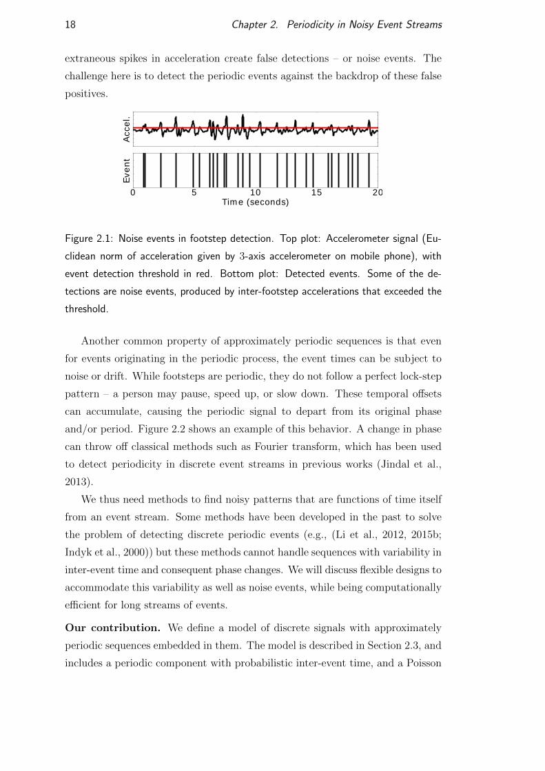
18 Chapter 2. Periodicity in Noisy Event Streams
extraneous spikes in acceleration create false detections – or noise events. The
challenge here is to detect the periodic events against the backdrop of these false
positives.
Figure 2.1: Noise events in footstep detection. Top plot: Accelerometer signal (Eu-
clidean norm of acceleration given by 3-axis accelerometer on mobile phone), with
event detection threshold in red. Bottom plot: Detected events. Some of the de-
tections are noise events, produced by inter-footstep accelerations that exceeded the
threshold.
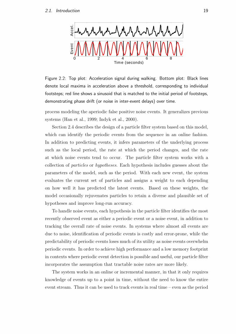
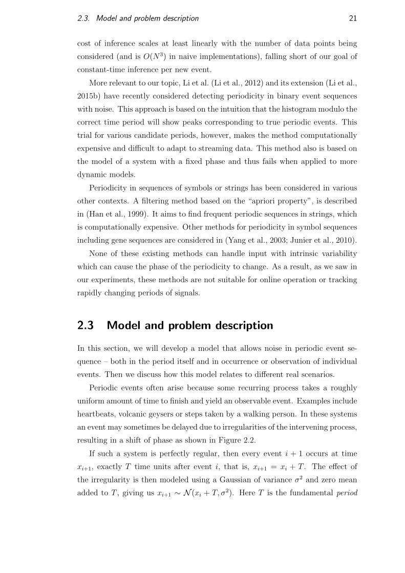
Another common property of approximately periodic sequences is that even
for events originating in the periodic process, the event times can be subject to
noise or drift. While footsteps are periodic, they do not follow a perfect lock-step
pattern – a person may pause, speed up, or slow down. These temporal offsets
can accumulate, causing the periodic signal to depart from its original phase
and/or period. Figure 2.2 shows an example of this behavior. A change in phase
can throw off classical methods such as Fourier transform, which has been used
to detect periodicity in discrete event streams in previous works (Jindal et al.,
2013).
We thus need methods to find noisy patterns that are functions of time itself
from an event stream. Some methods have been developed in the past to solve
the problem of detecting discrete periodic events (e.g., (Li et al., 2012, 2015b;
Indyk et al., 2000)) but these methods cannot handle sequences with variability in
inter-event time and consequent phase changes. We will discuss flexible designs to
accommodate this variability as well as noise events, while being computationally
efficient for long streams of events.
Our contribution. We define a model of discrete signals with approximately
periodic sequences embedded in them. The model is described in Section 2.3, and
includes a periodic component with probabilistic inter-event time, and a Poisson
2.1. Introduction 19
Figure 2.2: Top plot: Acceleration signal during walking. Bottom plot: Black lines
denote local maxima in acceleration above a threshold, corresponding to individual
footsteps; red line shows a sinusoid that is matched to the initial period of footsteps,
demonstrating phase drift (or noise in inter-event delays) over time.
process modeling the aperiodic false positive noise events. It generalizes previous
systems (Han et al., 1999; Indyk et al., 2000).
Section 2.4 describes the design of a particle filter system based on this model,
which can identify the periodic events from the sequence in an online fashion.
In addition to predicting events, it infers parameters of the underlying process
such as the local period, the rate at which the period changes, and the rate
at which noise events tend to occur. The particle filter system works with a
collection of particles or hypotheses. Each hypothesis includes guesses about the
parameters of the model, such as the period. With each new event, the system
evaluates the current set of particles and assigns a weight to each depending
on how well it has predicted the latest events. Based on these weights, the
model occasionally rejuvenates particles to retain a diverse and plausible set of
hypotheses and improve long-run accuracy.
To handle noise events, each hypothesis in the particle filter identifies the most
recently observed event as either a periodic event or a noise event, in addition to
tracking the overall rate of noise events. In systems where almost all events are
due to noise, identification of periodic events is costly and error-prone, while the
predictability of periodic events loses much of its utility as noise events overwhelm
periodic events. In order to achieve high performance and a low memory footprint
in contexts where periodic event detection is possible and useful, our particle filter
incorporates the assumption that tractable noise rates are more likely.
The system works in an online or incremental manner, in that it only requires
knowledge of events up to a point in time, without the need to know the entire
event stream. Thus it can be used to track events in real time – even as the period
20 Chapter 2. Periodicity in Noisy Event Streams
changes. We show it can operate accurately with relatively few particles and thus
can be used at a low computational cost to analyze large volumes of data in a
single pass. The particle filter processes events as they occur, and incurs no cost
for the quiet periods between them. Thus the cost of the method depends only
on the number of events, and is independent of the total duration of the event
sequence or the sampling rate.
Experiments in Section 2.5 show that the system can accurately estimate the
period of an event-generating process on both synthetic and real-world data. Ex-
isting methods are not designed to handle shifts in phase (Figure 2.2) and noise,
as a result, they perform relatively poorly in these cases. Each hypothesis in-
cludes expectations about when future periodic events will occur, so the system
can be used to predict upcoming events. Our experiments show that these pre-
dictions are accurate and robust to noise and changing periods. Moreover, the
experiments show that our system works well with sparse data, converging to
accurate estimates after observing only a few events.
2.2 Related works
Time series analysis has traditionally considered real-valued functions. Fourier
transform is a natural tool for detecting periodic patterns in real-valued signals,
and has also been applied to detect periodicity in binary event streams (Jindal
et al., 2013). However, as observed in (Li et al., 2012), it does not perform well
in data with noise, missing signals and other errors. It also does not lend itself to
online inference, which is one of our main desiderata. Further, Fourier transform
aims to fit a global phase and periodicity to the data. In our model, where
phase can drift, the signal can easily go out of phase with the basic sine wave
(Figure 2.2).
A sketch based approach in (Indyk et al., 2000) uses random linear projec-
tion over windows of time series data to compress them for easier comparison.
This makes comparison between windows easier, but does not easily extend to
detecting periodic events at arbitrarily large scales. More recently, Gaussian pro-
cesses with periodic and Fourier kernels have been used to detect such periodic
patterns (Ghassemi and Diesenroth, 2014; Osborne et al., 2008). These meth-
ods can detect periodic relationships in real-valued signals, but it is unclear how
they might be extended to accommodate point events or online inference; the
2.3. Model and problem description 21
cost of inference scales at least linearly with the number of data points being
considered (and is O(N3) in naive implementations), falling short of our goal of
constant-time inference per new event.
More relevant to our topic, Li et al. (Li et al., 2012) and its extension (Li et al.,
2015b) have recently considered detecting periodicity in binary event sequences
with noise. This approach is based on the intuition that the histogram modulo the
correct time period will show peaks corresponding to true periodic events. This
trial for various candidate periods, however, makes the method computationally
expensive and difficult to adapt to streaming data. This method also is based on
the model of a system with a fixed phase and thus fails when applied to more
dynamic models.
Periodicity in sequences of symbols or strings has been considered in various
other contexts. A filtering method based on the “apriori property”, is described
in (Han et al., 1999). It aims to find frequent periodic sequences in strings, which
is computationally expensive. Other methods for periodicity in symbol sequences
including gene sequences are considered in (Yang et al., 2003; Junier et al., 2010).
None of these existing methods can handle input with intrinsic variability
which can cause the phase of the periodicity to change. As a result, as we saw in
our experiments, these methods are not suitable for online operation or tracking
rapidly changing periods of signals.
2.3 Model and problem description
In this section, we will develop a model that allows noise in periodic event se-
quence – both in the period itself and in occurrence or observation of individual
events. Then we discuss how this model relates to different real scenarios.
Periodic events often arise because some recurring process takes a roughly
uniform amount of time to finish and yield an observable event. Examples include
heartbeats, volcanic geysers or steps taken by a walking person. In these systems
an event may sometimes be delayed due to irregularities of the intervening process,
resulting in a shift of phase as shown in Figure 2.2.
If such a system is perfectly regular, then every event i + 1 occurs at time
xi+1, exactly T time units after event i, that is, xi+1 = xi + T . The effect of
the irregularity is then modeled using a Gaussian of variance σ2 and zero mean
added to T , giving us xi+1 ∼ N (xi + T, σ2). Here T is the fundamental period
22 Chapter 2. Periodicity in Noisy Event Streams
or inter-event interval parameter, while σ can be seen as the “noisiness” of the
period over time.
Other than the intrinsic irregularity of the process, the data can reflect noise
events. Noise events may either come from the observation mechanism affecting
both record of true events as we have seen in Figure 2.1, or it may represent a
different or spurious source of events.
We model this noise sequence as a Poisson process, i.e., a sequence of events
z1, z2, ... where zi+1 = zi + δ, and δ follows an exponential distribution with rate
parameter λ; a higher lambda implies a greater rate, or shorter expected durations
between false positive events.
Thus in our model, the overall sequence y = y1, y2, . . . can be partitioned into
two subsequences1:
• A sequence x of periodic events, where xi+1 ∼ N (xi + T, σ2).
• A sequence z of noise events given by zi+1 = zi + δ, where δ follows an
exponential distribution with an expectation of (λ)−1, for a rate parameter
λ > 0.
Problem statement. Given a sequence of event times y1:n = y1, . . . , yn, we
wish to infer the period T , which is the fundamental parameter that describes
the behavior of the system. We would also like to know the parameters σ and λ
that determine the extent and nature of the noise in the system.
As an additional feature, we want the algorithm to be online, meaning that
it processes the sequence one item at a time, updating its estimates with each
input without requiring that the system store or process the full event history.
The ideal algorithm will make inferences with O(1) time and memory complexity
after each event, and can thus remain responsive even after processing arbitrarily
large numbers of events.
Generality of the model and local fit with input. This model incorporates
quite general scenarios. It does not make any assumption about there being a set
of “true” signal events to detect as opposed to observational noise. It assumes that
all events may be generated by the same underlying process, and aims to detect
the presence of a periodic subsequence. The Gaussian distribution of inter-event
1A subsequence of a sequence is a subset of the events, not necessarily contiguous, in thesame order as in the original sequence.
2.3. Model and problem description 23
time represents a sum of unknown variables that may cause the local variations
in the period.
As shown in Figure 2.1, the threshold for an “event” determines the noise rate.
It is possible to set a high threshold to ensure very few noise events, at the risk
of missing some fraction of periodic events. However, lower thresholds are more
desirable – they may include more noise, but will not miss the periodic events.
Our model is designed with this setup in mind – that periodic event information
is preserved, even at the cost of more noise events. The parameter λ as part of
the hypothesis learns this noise rate. Poisson processes are commonly used for
such models, as they only assume that the noise occurs at a certain uniform rate
in any temporal locality.
Note that the system operates in terms of a set of evolving hypothesis and
can adapt to changing model parameters online as the system behavior changes.
Thus, it is not required that the model fits the global data over long periods
of time, only that it fits the system approximately, over any short period of
time. Experiments show that in fact this model successfully adapts to periodic
events and tracks them closely with changes in the system. Its performance
remains consistent when the noise and inter-event variability are generated using
distributions other than the ones assumed in the model.
Discussion and variations of the model. There are various common sce-
narios where periodic events are generated by processes that are special cases or
variations on the model above. The simplest is what we will call strict periodicity,
where successive events are separated by an exact time interval T , such as clock
ticks, or events tied to clock-like sequences. Formally, xi = φ + iT , if all events
are due to a strictly periodic process. We get this behavior in our model above
by setting σ = λ = 0.
Strict periodicities are easy to capture, by simply observing the interval be-
tween successive events. A variant of this is partial periodicity, where a strict
periodic function is mixed with noise. This was considered in (Han et al., 1999).
Certain sequences like heartbeats or volcanic geysers satisfy λ = 0;σ > 0 –
they are not tied to a clock, but depend on a build up in the intervening process
that can have some variability, and change in phase or even dynamic change in
the period itself.
There are systems where noise in the periodicity exists, that is σ > 0, but
phase does not not change. Example would be daily activities of a person –

24 Chapter 2. Periodicity in Noisy Event Streams
such as checking the news in the morning – which may not have a strict inter-
event time, but still around a particular time in the morning. These can be
modeled by adding observational noise to strict periodicity: xi ∼ N (φ+ iT, σ2).
The variation in inter-event time does not affect the phase φ here. This type of
sequences have been addressed in a recent work (Li et al., 2012). The approach
there is to consider the histogram of events modulo a number W , which produces
a pronounced peak at the correct value of W = T . We discuss this and other
related methods in Section 4.2.
2.4 Particle filter design
In this section, we describe a particle filter based system to detect periodicity in
noisy and approximately periodic event sequences. The next subsection briefly
summarizes particle filters, which form the foundation of our approach, and lists
our notations. Following this, we describe the details of our design to adapt
particle filters to the current problem.
2.4.1 Particle filters and importance sampling
Particle filters, or sequential Monte Carlo methods, are a popular family of on-
line methods for making inferences about latent variables in noisy environments.
They have been applied to diverse problems, including locating and tracking ob-
jects using sensor data (e.g., (Stewart and McCarty, 1992)), machine vision (e.g.,
(Nummiaro et al., 2003)), and natural language processing (e.g., (Canini et al.,
2009)).
The essential idea is that each particle is a point sample in the space of pos-
sibilities of all the parameters in question. We interchangeably use the term
hypothesis to mean that each particle is one of our guesses of the true configura-
tion of the system.
Our goal is to determine the period T of an approximately periodic sequence.
In probabilistic terms, we want to obtain a posterior distribution over possible
values of Tn: the period after the nth event, given a vector of observed event
timestamps y1:n = {y1, ..., yn} up to that point. The period is not the only
salient feature of the event-generating process, so we will use hn to denote the
ensemble of features, which includes the period, variance σ2, rate of noise events
2.4. Particle filter design 25
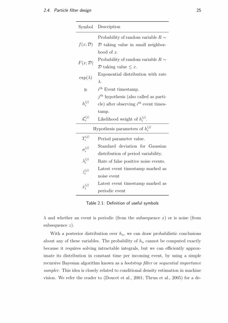
Symbol Description
f(x;D)
Probability of random variable R ∼D taking value in small neighbor-
hood of x.
F (x;D)Probability of random variable R ∼D taking value ≤ x.
exp(λ)Exponential distribution with rate
λ.
yi ith Event timestamp.
h(j)i
jth hypothesis (also called as parti-
cle) after observing ith event times-
tamp.
L(j)i Likelihood weight of h
(j)i .
Hypothesis parameters of h(j)i
T(j)i Period parameter value.
σ(j)i
Standard deviation for Gaussian
distribution of period variability.
λ(j)i Rate of false positive noise events.
z(j)i
Latest event timestamp marked as
noise event
x(j)i
Latest event timestamp marked as
periodic event
Table 2.1: Definition of useful symbols
λ and whether an event is periodic (from the subsequence x) or is noise (from
subsequence z).
With a posterior distribution over hn, we can draw probabilistic conclusions
about any of these variables. The probability of hn cannot be computed exactly
because it requires solving intractable integrals, but we can efficiently approx-
imate its distribution in constant time per incoming event, by using a simple
recursive Bayesian algorithm known as a bootstrap filter or sequential importance
sampler. This idea is closely related to conditional density estimation in machine
vision. We refer the reader to (Doucet et al., 2001; Thrun et al., 2005) for a de-
26 Chapter 2. Periodicity in Noisy Event Streams
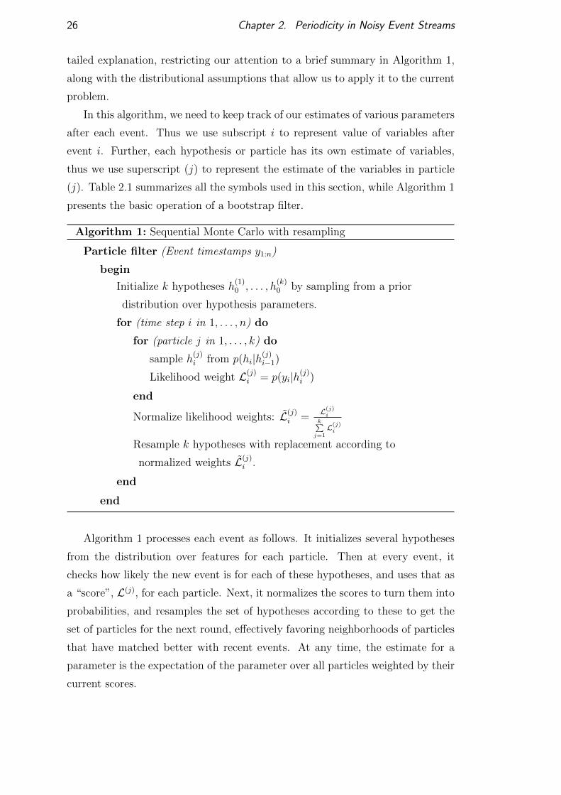
tailed explanation, restricting our attention to a brief summary in Algorithm 1,
along with the distributional assumptions that allow us to apply it to the current
problem.
In this algorithm, we need to keep track of our estimates of various parameters
after each event. Thus we use subscript i to represent value of variables after
event i. Further, each hypothesis or particle has its own estimate of variables,
thus we use superscript (j) to represent the estimate of the variables in particle
(j). Table 2.1 summarizes all the symbols used in this section, while Algorithm 1
presents the basic operation of a bootstrap filter.
Algorithm 1: Sequential Monte Carlo with resampling
Particle filter (Event timestamps y1:n)
begin
Initialize k hypotheses h(1)0 , . . . , h
(k)0 by sampling from a prior
distribution over hypothesis parameters.
for (time step i in 1, . . . , n) do
for (particle j in 1, . . . , k) do
sample h(j)i from p(hi|h(j)
i−1)
Likelihood weight L(j)i = p(yi|h(j)
i )
end
Normalize likelihood weights: L(j)i =
L(j)i
k∑j=1L(j)i
Resample k hypotheses with replacement according to
normalized weights L(j)i .
end
end
Algorithm 1 processes each event as follows. It initializes several hypotheses
from the distribution over features for each particle. Then at every event, it
checks how likely the new event is for each of these hypotheses, and uses that as
a “score”, L(j), for each particle. Next, it normalizes the scores to turn them into
probabilities, and resamples the set of hypotheses according to these to get the
set of particles for the next round, effectively favoring neighborhoods of particles
that have matched better with recent events. At any time, the estimate for a
parameter is the expectation of the parameter over all particles weighted by their
current scores.

2.4. Particle filter design 27
2.4.2 Particle filter for discovering periodicity
A hypothesis hn contains the estimated characteristics of the periodic signal after
n events. The periodic characteristics are specified using the period Tn, and stan-
dard deviation σn for Gaussian distribution of period variability. Our hypothesis
hn also includes the last periodic event xn in the sequence. We have included
the rate of background noise events λn, and the timestamp of the last event that
was attributed to noise, zn in our definition of hn. We will use i to index event
timestamp, yi, where 1 ≤ i ≤ n.
Under this model, each event yi originates from either the periodic signal
or false positive noise. We introduce ri ∈ {0, 1} to track event provenance,
where ri = 1 represents the case where the ith event comes from the periodic
process. This auxiliary variable facilitates efficient inference: using ri, we ob-
tain a closed-form solution for the density of periodic events conditional on the
last periodic event, and noise density conditional on the last event. Calculat-
ing P (ri|y1:i, h0:i−1, r1:i−1) exactly is expensive, as the number of states involved
increases exponentially as we observe more events, but we can augment our sam-
pling procedure to reflect the posterior distribution of ri. For simplicity we omit
(j) superscripts where they are clear from context.
The bootstrap particle filter algorithm requires us to specify three probability
distributions:
• A prior over hypotheses for initialization of h(j)0 .
• A likelihood function adjusting the weight of a hypothesis given observed
events.
• A distribution defining how hypotheses change between events.
We specify the distributions as follows:
Priors. For each hypothesis h(j) we sample the initial period T(j)0 and noise
event rate λ(j)0 from exponential distributions, and sample the standard deviation
σ(j)0 uniformly from the interval [0, T
(j)0 ]. At the initialization stage, we know
nothing about the periodicity value or noise event rate other than that they are
positive, thus we use exponential distribution as a maximum entropy guess for
the distribution. Both x(j)0 and z
(j)0 are assumed to start at zero.
Likelihood weighting. Given a hypothesis hi, the likelihood of event i occurring
28 Chapter 2. Periodicity in Noisy Event Streams
at time yi is equal to L =∑
ri∈0,1 p(yi, ri|hi). The periodic signal’s contribution
to this sum is Lper = p(yi, ri = 1|hi), and is the product of two terms:
• Density function from the previous periodic event, assuming that xi−1 is
known. Since the time of a periodic event is subject to additive Gaussian
noise, we represent this density as
p(yi|h(j)i ) = N (T
(j)i + x
(j)i−1, σ
(j)i ). (2.1)
• A term based on the observation that ri = 0 if and only if there are zero
noise events in the time between zi−1 and yi, inclusive. If a Poisson process
generates noise events, then that probability is e−λi(yi−zi−1).
The false positive noise’s contribution to the total likelihood is Lbg = p(yi, ri =
0|hi). Here, we have a product of two terms:
• An exponential distribution, with its origin at zi and a rate equal to the
noise rate.
• The cumulative probability that no periodic event occurred between xi−1
and yi. We approximate this probability by the complementary cumulative
density of periodic events between yi and xi−1 by evaluating the comple-
mentary cumulative density function for the distribution in Equation 2.1.
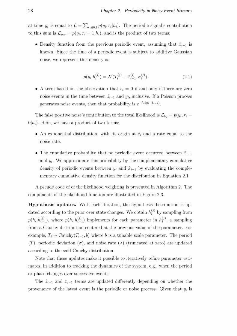
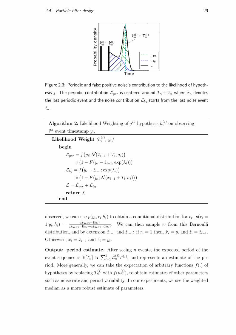
A pseudo code of of the likelihood weighting is presented in Algorithm 2. The
components of the likelihood function are illustrated in Figure 2.3.
Hypothesis updates. With each iteration, the hypothesis distribution is up-
dated according to the prior over state changes. We obtain h(j)i by sampling from
p(hi|h(j)i−1), where p(hi|h(j)
i−1) implements for each parameter in h(j)i , a sampling
from a Cauchy distribution centered at the previous value of the parameter. For
example, Ti ∼ Cauchy(Ti−1, b) where b is a tunable scale parameter. The period
(T ), periodic deviation (σ), and noise rate (λ) (truncated at zero) are updated
according to the said Cauchy distribution.
Note that these updates make it possible to iteratively refine parameter esti-
mates, in addition to tracking the dynamics of the system, e.g., when the period
or phase changes over successive events.
The zi−1 and xi−1 terms are updated differently depending on whether the
provenance of the latest event is the periodic or noise process. Given that yi is
2.4. Particle filter design 29
Figure 2.3: Periodic and false positive noise’s contribution to the likelihood of hypoth-
esis j. The periodic contribution Lper is centered around Tn + xn where xn denotes
the last periodic event and the noise contribution Lbg starts from the last noise event
zn.
Algorithm 2: Likelihood Weighting of jth hypothesis h(j)i on observing
ith event timestamp yi.
Likelihood Weight (h(j)i , yi)
begin
Lper = f(yi;N (xi−1 + Ti, σi)
)×(1− F
(yi − zi−1; exp(λi)))
Lbg = f(yi − zi−1; exp(λi)
)×(1− F
(yi;N (xi−1 + Ti, σi)
))L = Lper + Lbgreturn L
end
observed, we can use p(yi, ri|hi) to obtain a conditional distribution for ri: p(ri =
1|yi, hi) = p(yi,ri=1|hi)p(yi,ri=1|hi)+p(yi,ri=0|hi) . We can then sample ri from this Bernoulli
distribution, and by extension xi−1 and zi−1: if ri = 1 then, xi = yi and zi = zi−1.
Otherwise, xi = xi−1 and zi = yi.
Output: period estimate. After seeing n events, the expected period of the
event sequence is E[Tn] ≈∑k
i=1 L(j)n T (j), and represents an estimate of the pe-
riod. More generally, we can take the expectation of arbitrary functions f(.) of
hypotheses by replacing T(j)n with f(h
(j)n ), to obtain estimates of other parameters
such as noise rate and period variability. In our experiments, we use the weighted
median as a more robust estimate of parameters.
30 Chapter 2. Periodicity in Noisy Event Streams
2.4.3 Practical optimizations for noisy environments
The algorithm presented in the previous section can detect the period of a noisy
sequence of events, but can require a large number of hypotheses to do so reliably;
the particle filter needs a considerable number of hypotheses to ensure that several
occupy high-probability regions of the parameter space. If we use a small number
of hypotheses, then the particle filter will occasionally provide poor or high-
variance estimates, especially when the period or dynamics are extreme or a
priori unlikely. In this section, we present a modification our basic algorithm
that preserves accuracy while using fewer hypotheses.
A pragmatic observation from an end-user’s point of view is that if the number
of noise events in a sequence is much greater than the number of periodic events,
then the period value of the signal is not useful for predicting future events, and
periodic event detection may become infeasible. Motivated by this observation,
we can modify the likelihood weighting strategy for the previous algorithm to
capture the assumption that we are facing an estimation problem for which there
exists a useful solution. In so doing, we improve our ability to obtain useful
solutions if they exist, and incur negligible costs if they do not.
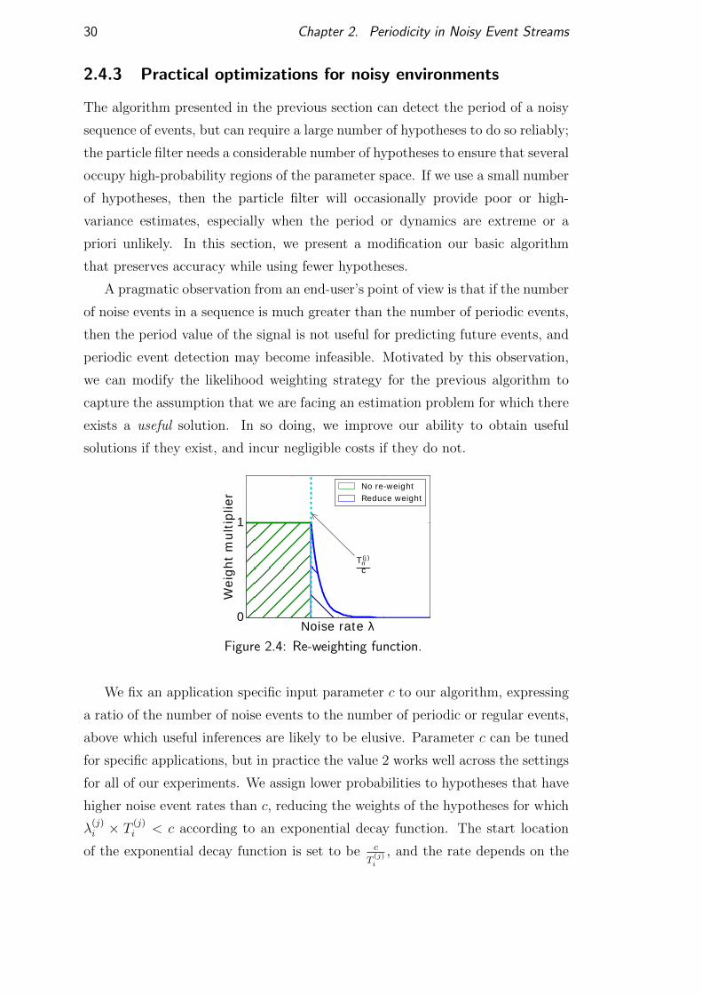
Figure 2.4: Re-weighting function.
We fix an application specific input parameter c to our algorithm, expressing
a ratio of the number of noise events to the number of periodic or regular events,
above which useful inferences are likely to be elusive. Parameter c can be tuned
for specific applications, but in practice the value 2 works well across the settings
for all of our experiments. We assign lower probabilities to hypotheses that have
higher noise event rates than c, reducing the weights of the hypotheses for which
λ(j)i × T
(j)i < c according to an exponential decay function. The start location
of the exponential decay function is set to be c
T(j)i
, and the rate depends on the

2.5. Experimental evaluation 31
importance of the assumption of limiting noise rate. We multiply the likelihood
of a hypothesis derived as described in the previous section by a value drawn
from a function as represented in Figure 2.4. With this strategy, we ensure low
weights for the hypotheses which have large periods and high noise event rates
that would lead to poor predictive accuracy.
2.5 Experimental evaluation
We tested the performance of our particle filter and compared it with existing
ideas on real human gait data and human pulse data. We also created several
sets of artificial data with different values of intrinsic variability, noise event rate,
and period to precisely characterize the detection accuracy. Overall, we found
that:
• In presence of noise events and phase drifts the particle filter method out-
performs other techniques in accuracy.
• With higher noise event rates and phase drift, only the particle filter pro-
duces reasonably accurate and reliable results.
• The particle filter method can operate with a reasonable and constant num-
ber of about 256 particles to give good results.
• The particle filter runs more efficiently than competing methods, and thus
is suitable for operation in an online environment to produce increasingly
accurate results.
• On data with rapidly changing periodicity, the method can track the period
closely. We show this by applying the technique to human step data to
determine changing gait rate.
• The method applied to real data such as human pulse and gait data accu-
rately detects periodicity.
The following subsections first describe the competing techniques for period-
icity detection, and then the detailed experimental results.
32 Chapter 2. Periodicity in Noisy Event Streams
2.5.1 Comparison algorithms
The following popular methods for detecting periodicity are compared with the
particle filter algorithm.
Fourier Transform: The frequency with highest spectral energy in Fast
Fourier Transform algorithm is a reasonable candidate for the true frequency of
the system. This technique has been used in the past as a practical method for
detecting periodicity (Jindal et al., 2013).
Autocorrelation: The cross-correlation of the input signal with the signal
itself with different amounts of offsets, thus building the autocorrelogram can
be used to find period of a signal. The delay of the signal where the cross-
correlation value reaches its maximum value can then be treated as the period of
the signal (Vlachos et al., 2005). A linear search on period values is required to
find this maximum.
Segmentation based algorithm: The method described in (Li et al., 2012)
detects periodicity in face of approximate periodicity and noise, as described in
Section 2.3. This algorithm operates by checking all possible periods by com-
puting the histogram of events modulo the period, and looking for a “peak” in
this histogram. This checking of all possible periods makes it inefficient on large
datasets.
2.5.2 Sensitivity to noise and model parameters
To gain understanding of the basic operation of the system in noisy environments
with variability in period and presence of noise events requires data with precisely
known values of these parameters. We thus simulated artificial data based on the
models described in Section 2.3.
2.5.2.1 Generation of synthetic data
With fixed values for parameters: period T , deviation of periodic events σ, and
noise event rate λ, we generated two separate sequences: the periodic events and
the noise events, and merged them in sorted order.
Periodic event sequence (x). The first periodic event x0 is set to 0. Each
subsequent periodic event i is designated to occur at time xi given by xi =
xi−1 + δper. The distance between two consecutive periodic events, δper is drawn
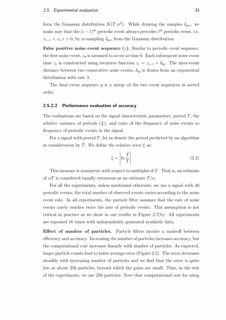
2.5. Experimental evaluation 33
form the Gaussian distribution N (T, σ2). While drawing the samples δper, we
make sure that the (i− 1)th periodic event always precedes ith periodic event, i.e.
xi−1 < xi, i > 0, by re-sampling δper from the Gaussian distribution.
False positive noise event sequence (z). Similar to periodic event sequence,
the first noise event, z0 is assumed to occur at time 0. Each subsequent noise event
time zi is constructed using recursive function zi = zi−1 + δbg. The inter-event
distance between two consecutive noise events, δbg is drawn from an exponential
distribution with rate λ.
The final event sequence y is a merge of the two event sequences in sorted
order.
2.5.2.2 Performance evaluation of accuracy
The evaluations are based on the signal characteristic parameters: period T , the
relative variance of periods ( σT
), and ratio of the frequency of noise events to
frequency of periodic events in the signal.
For a signal with period T , let us denote the period predicted by an algorithm
in consideration by T . We define the relative error ξ as:
ξ =
∣∣∣∣∣ln TT∣∣∣∣∣ (2.2)
This measure is symmetric with respect to multiples of T . That is, an estimate
of αT is considered equally erroneous as an estimate T/α.
For all the experiments, unless mentioned otherwise, we use a signal with 40
periodic events; the total number of observed events varies according to the noise
event rate. In all experiments, the particle filter assumes that the rate of noise
events rarely reaches twice the rate of periodic events. This assumption is not
critical in practice as we show in our results in Figure 2.7(b). All experiments
are repeated 16 times with independently generated synthetic data.
Effect of number of particles. Particle filters involve a tradeoff between
efficiency and accuracy. Increasing the number of particles increases accuracy, but
the computational cost increases linearly with number of particles. As expected,
larger particle counts lead to lower average error (Figure 2.5). The error decreases
steadily with increasing number of particles and we find that the error is quite
low at about 256 particles, beyond which the gains are small. Thus, in the rest
of the experiments, we use 256 particles. Note that computational cost for using
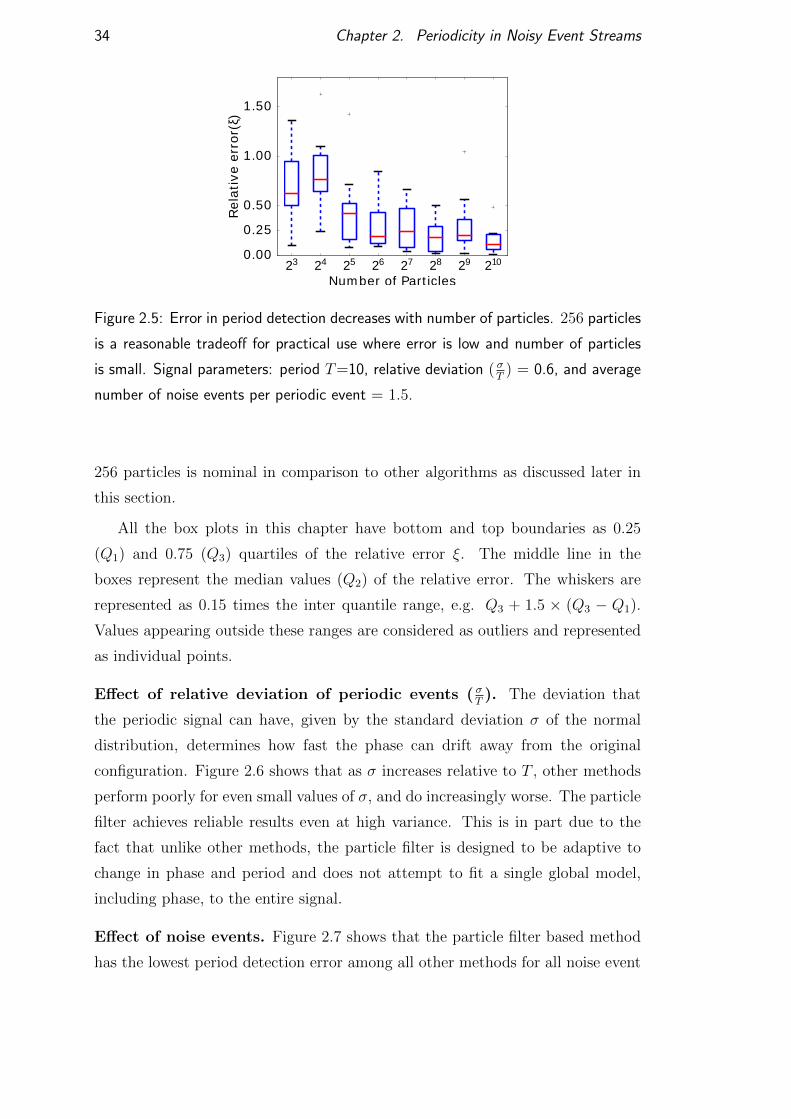
34 Chapter 2. Periodicity in Noisy Event Streams
Figure 2.5: Error in period detection decreases with number of particles. 256 particles
is a reasonable tradeoff for practical use where error is low and number of particles
is small. Signal parameters: period T=10, relative deviation ( σT
) = 0.6, and average
number of noise events per periodic event = 1.5.
256 particles is nominal in comparison to other algorithms as discussed later in
this section.
All the box plots in this chapter have bottom and top boundaries as 0.25
(Q1) and 0.75 (Q3) quartiles of the relative error ξ. The middle line in the
boxes represent the median values (Q2) of the relative error. The whiskers are
represented as 0.15 times the inter quantile range, e.g. Q3 + 1.5 × (Q3 − Q1).
Values appearing outside these ranges are considered as outliers and represented
as individual points.
Effect of relative deviation of periodic events ( σT). The deviation that
the periodic signal can have, given by the standard deviation σ of the normal
distribution, determines how fast the phase can drift away from the original
configuration. Figure 2.6 shows that as σ increases relative to T , other methods
perform poorly for even small values of σ, and do increasingly worse. The particle
filter achieves reliable results even at high variance. This is in part due to the
fact that unlike other methods, the particle filter is designed to be adaptive to
change in phase and period and does not attempt to fit a single global model,
including phase, to the entire signal.
Effect of noise events. Figure 2.7 shows that the particle filter based method
has the lowest period detection error among all other methods for all noise event
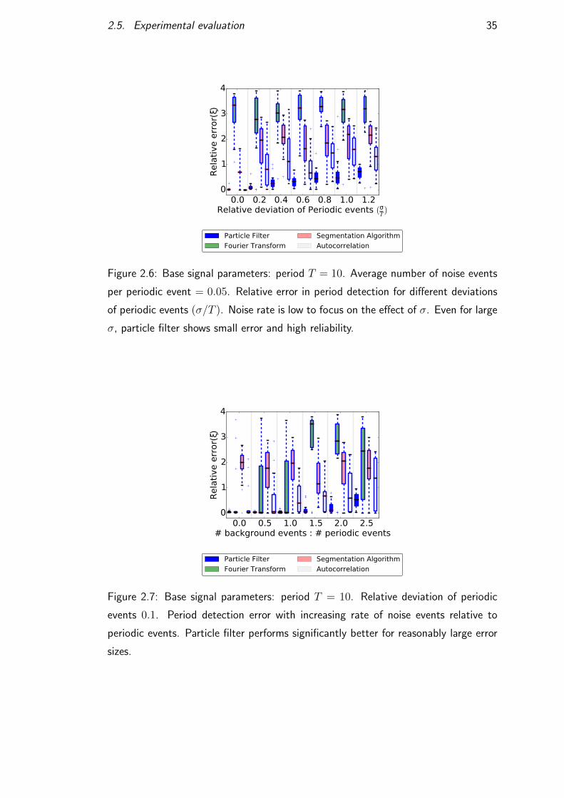
2.5. Experimental evaluation 35
Figure 2.6: Base signal parameters: period T = 10. Average number of noise events
per periodic event = 0.05. Relative error in period detection for different deviations
of periodic events (σ/T ). Noise rate is low to focus on the effect of σ. Even for large
σ, particle filter shows small error and high reliability.
Figure 2.7: Base signal parameters: period T = 10. Relative deviation of periodic
events 0.1. Period detection error with increasing rate of noise events relative to
periodic events. Particle filter performs significantly better for reasonably large error
sizes.
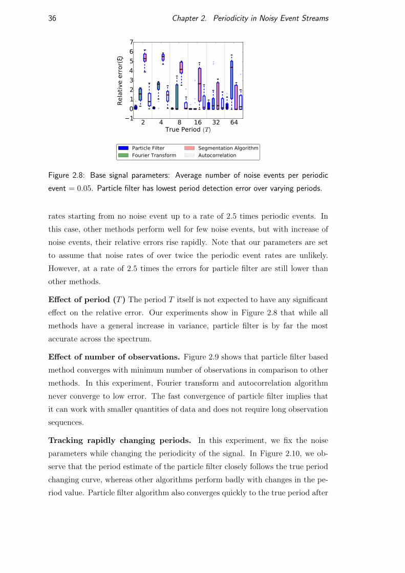
36 Chapter 2. Periodicity in Noisy Event Streams
Figure 2.8: Base signal parameters: Average number of noise events per periodic
event = 0.05. Particle filter has lowest period detection error over varying periods.
rates starting from no noise event up to a rate of 2.5 times periodic events. In
this case, other methods perform well for few noise events, but with increase of
noise events, their relative errors rise rapidly. Note that our parameters are set
to assume that noise rates of over twice the periodic event rates are unlikely.
However, at a rate of 2.5 times the errors for particle filter are still lower than
other methods.
Effect of period (T ) The period T itself is not expected to have any significant
effect on the relative error. Our experiments show in Figure 2.8 that while all
methods have a general increase in variance, particle filter is by far the most
accurate across the spectrum.
Effect of number of observations. Figure 2.9 shows that particle filter based
method converges with minimum number of observations in comparison to other
methods. In this experiment, Fourier transform and autocorrelation algorithm
never converge to low error. The fast convergence of particle filter implies that
it can work with smaller quantities of data and does not require long observation
sequences.
Tracking rapidly changing periods. In this experiment, we fix the noise
parameters while changing the periodicity of the signal. In Figure 2.10, we ob-
serve that the period estimate of the particle filter closely follows the true period
changing curve, whereas other algorithms perform badly with changes in the pe-
riod value. Particle filter algorithm also converges quickly to the true period after
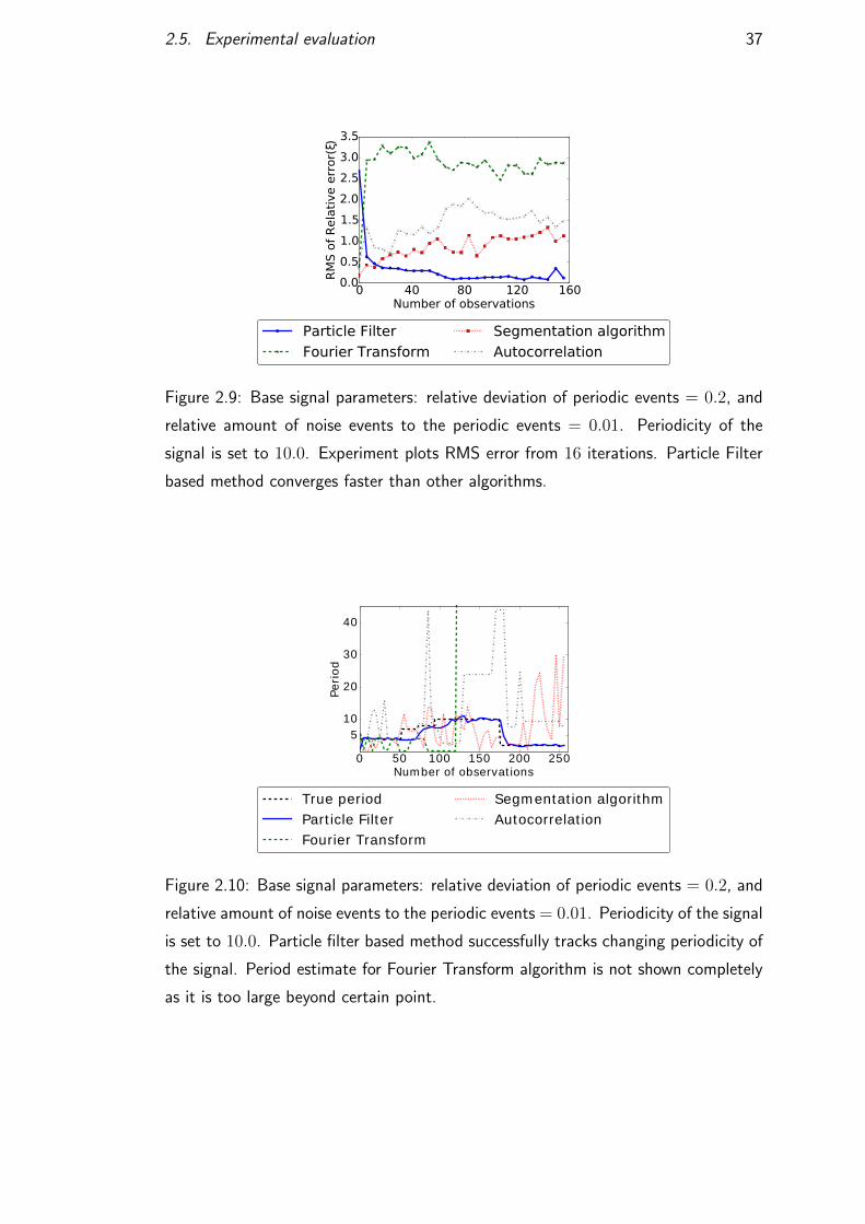
2.5. Experimental evaluation 37
Figure 2.9: Base signal parameters: relative deviation of periodic events = 0.2, and
relative amount of noise events to the periodic events = 0.01. Periodicity of the
signal is set to 10.0. Experiment plots RMS error from 16 iterations. Particle Filter
based method converges faster than other algorithms.
Figure 2.10: Base signal parameters: relative deviation of periodic events = 0.2, and
relative amount of noise events to the periodic events = 0.01. Periodicity of the signal
is set to 10.0. Particle filter based method successfully tracks changing periodicity of
the signal. Period estimate for Fourier Transform algorithm is not shown completely
as it is too large beyond certain point.
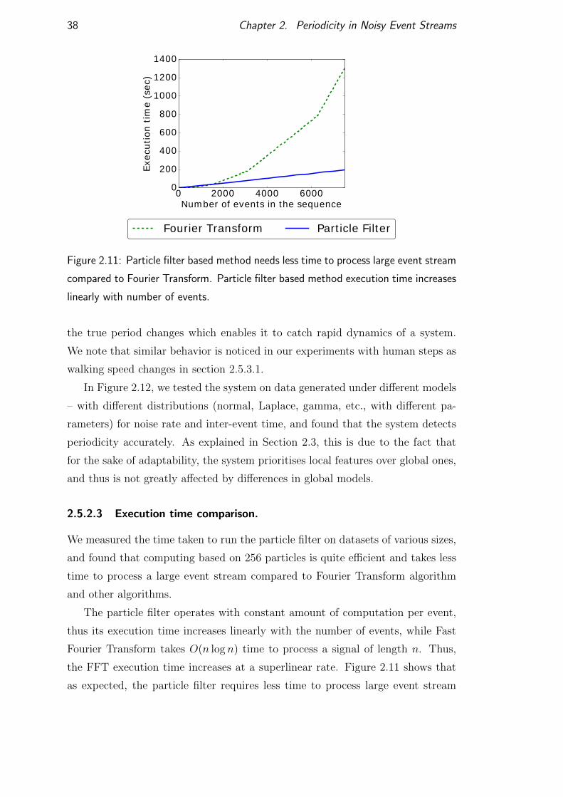
38 Chapter 2. Periodicity in Noisy Event Streams
Figure 2.11: Particle filter based method needs less time to process large event stream
compared to Fourier Transform. Particle filter based method execution time increases
linearly with number of events.
the true period changes which enables it to catch rapid dynamics of a system.
We note that similar behavior is noticed in our experiments with human steps as
walking speed changes in section 2.5.3.1.
In Figure 2.12, we tested the system on data generated under different models
– with different distributions (normal, Laplace, gamma, etc., with different pa-
rameters) for noise rate and inter-event time, and found that the system detects
periodicity accurately. As explained in Section 2.3, this is due to the fact that
for the sake of adaptability, the system prioritises local features over global ones,
and thus is not greatly affected by differences in global models.
2.5.2.3 Execution time comparison.
We measured the time taken to run the particle filter on datasets of various sizes,
and found that computing based on 256 particles is quite efficient and takes less
time to process a large event stream compared to Fourier Transform algorithm
and other algorithms.
The particle filter operates with constant amount of computation per event,
thus its execution time increases linearly with the number of events, while Fast
Fourier Transform takes O(n log n) time to process a signal of length n. Thus,
the FFT execution time increases at a superlinear rate. Figure 2.11 shows that
as expected, the particle filter requires less time to process large event stream
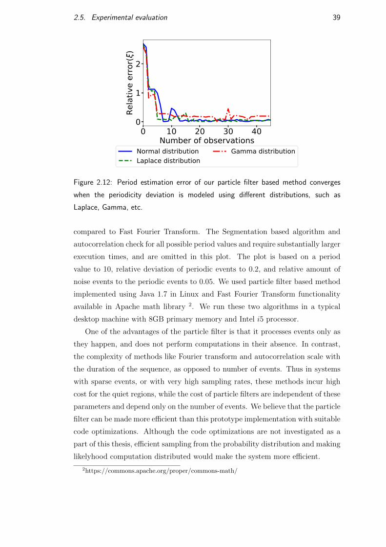
2.5. Experimental evaluation 39
0 10 20 30 40Number of observations
0
1
2
Rela
tive
erro
r()
Normal distributionLaplace distribution
Gamma distribution
Figure 2.12: Period estimation error of our particle filter based method converges
when the periodicity deviation is modeled using different distributions, such as
Laplace, Gamma, etc.
compared to Fast Fourier Transform. The Segmentation based algorithm and
autocorrelation check for all possible period values and require substantially larger
execution times, and are omitted in this plot. The plot is based on a period
value to 10, relative deviation of periodic events to 0.2, and relative amount of
noise events to the periodic events to 0.05. We used particle filter based method
implemented using Java 1.7 in Linux and Fast Fourier Transform functionality
available in Apache math library 2. We run these two algorithms in a typical
desktop machine with 8GB primary memory and Intel i5 processor.
One of the advantages of the particle filter is that it processes events only as
they happen, and does not perform computations in their absence. In contrast,
the complexity of methods like Fourier transform and autocorrelation scale with
the duration of the sequence, as opposed to number of events. Thus in systems
with sparse events, or with very high sampling rates, these methods incur high
cost for the quiet regions, while the cost of particle filters are independent of these
parameters and depend only on the number of events. We believe that the particle
filter can be made more efficient than this prototype implementation with suitable
code optimizations. Although the code optimizations are not investigated as a
part of this thesis, efficient sampling from the probability distribution and making
likelyhood computation distributed would make the system more efficient.
2https://commons.apache.org/proper/commons-math/
40 Chapter 2. Periodicity in Noisy Event Streams
2.5.3 Experiments on real datasets
We found that the particle filter can closely track changing periodicity in human
gait data in comparison to other algorithms and accurately predict next human
pulse event with low error.
2.5.3.1 Periodicity in human step data
We compared the performance of the particle filter based algorithm with other al-
gorithms described in subsection 2.5.1 for tracking changing periodicity in human
steps. We collected accelerometer signals using mobile phones while users walk
at their own pace, varying their walking speed between walking segments. An
accelerometer measures acceleration of a user giving a three dimensional signal
Sx, Sy, and Sz. The Euclidean norm represents the magnitude of the signal at
time t: St =√
(Sxt )2 + (Syt )2 + (Szt )2, followed by smoothing using a Gaussian
filter and normalizing around its mean. All peaks in the normalized signal above
a predefined threshold are considered as discrete step events. Taking different
values for threshold results in different rates of noise events as we have seen in
Figure 2.1. We calculated the ground truth of step periodicity as the average time
taken per step over a segment. A segment is the time duration when the user
conciously maintains his walking speed almost a constant. The data is annotated
by the user himself while walking. He presses a button in the app at the time of
changing walking speed; thus, the segments can be identified later. The ratio of
the duration of a segment and the number of steps in that segment denotes the
ground truth walking speed.
Tracking a single walking trace. Figure 2.13 shows that the estimated period
from the particle filter closely tracks the changing curve of ground truth step
periodicity as it changes between segments. Here we used the threshold as the
half of the standard deviation of the smoothed magnitude signal to detect step
events. Figure 2.14 shows that due to its local adaptive nature, the particle filter
has the lowest periodicity estimation error among all algorithms. Figure 2.15
shows the CDF of error over twelve traces collected from six different people.
The particle filter method is robust to different choices of thresholds for ex-
tracting step events from the accelerometer signal. This is shown in Figure 2.16
for different choices of threshold.
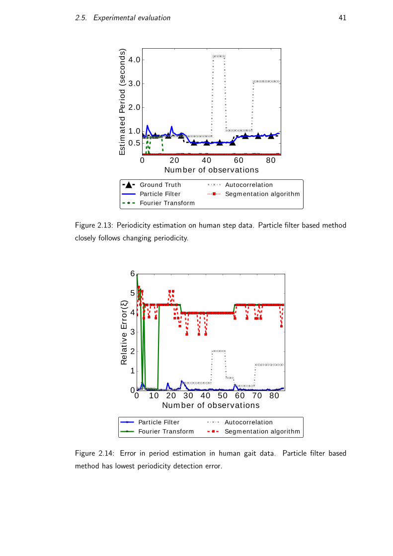
2.5. Experimental evaluation 41
Figure 2.13: Periodicity estimation on human step data. Particle filter based method
closely follows changing periodicity.
Figure 2.14: Error in period estimation in human gait data. Particle filter based
method has lowest periodicity detection error.
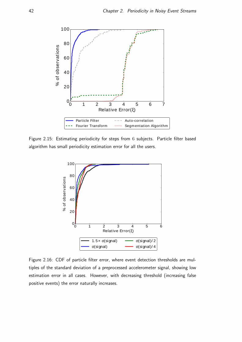
42 Chapter 2. Periodicity in Noisy Event Streams
Figure 2.15: Estimating periodicity for steps from 6 subjects. Particle filter based
algorithm has small periodicity estimation error for all the users.
Figure 2.16: CDF of particle filter error, where event detection thresholds are mul-
tiples of the standard deviation of a preprocessed accelerometer signal, showing low
estimation error in all cases. However, with decreasing threshold (increasing false
positive events) the error naturally increases.
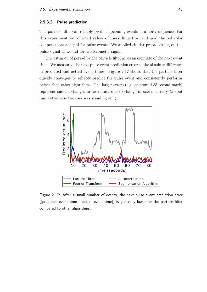
2.5. Experimental evaluation 43
2.5.3.2 Pulse prediction.
The particle filter can reliably predict upcoming events in a noisy sequence. For
this experiment we collected videos of users’ fingertips, and used the red color
component as a signal for pulse events. We applied similar preprocessing on the
pulse signal as we did for accelerometer signal.
The estimate of period by the particle filter gives an estimate of the next event
time. We measured the next pulse event prediction error as the absolute difference
in predicted and actual event times. Figure 2.17 shows that the particle filter
quickly converges to reliably predict the pulse event and consistently performs
better than other algorithms. The larger errors (e.g. at around 55 second mark)
represent sudden changes in heart rate due to change in user’s activity (a spot
jump otherwise the user was standing still).
Figure 2.17: After a small number of events, the next pulse event prediction error
(|predicted event time − actual event time|) is generally lower for the particle filter
compared to other algorithms.

Chapter 3
Private Sensing of Asynchronous
Event Sequences
In this chapter, we provide a rigorous study of the privacy of event timestamps,
which are particularly sensitive attributes. Our privacy approach is specially
tailored to discrete point events with varying rates and asynchronous operation,
which is shown to be more effective than existing synchronous methods. We
propose new privacy mechanisms, including temporal perturbation and inclusion
of fake events. These methods provide provable guarantees against the adversary
deducing time of events, identifying events with timing correlation attacks and
inferring temporal ordering of events. We describe the implementation of data
privatization as a system service on Android. Experiments on public datasets
and locally collected data show that the privacy mechanisms are found to protect
utility by preserving the overall distribution of events.
3.1 Introduction
Densely deployed sensors and IoT devices provide opportunities for large scale
monitoring of home, workplace and public domains (Chen et al., 2017; Ganti
et al., 2008). In the process of sharing and use of IoT data, protection of sensi-
tive information related to activities of an individual has become an important
research topic. In this paper, we consider the privacy issue in publishing times-
tamps of sensing events.
Consider sensors or mobile phones detecting specific events and activities of
users and later reporting these behavior statistics to a service provider for usage
45
46 Chapter 3. Private Sensing of Asynchronous Event Sequences
analysis. Timestamp information can imply correlation, association and causality
between events, and thus are sensitive attributes. An adversary who has access to
details of certain external events can cross-query the datasets and associate users
with external events. For example, timing information of online activities and
web browsing can be used to perform timing correlation attacks to deduce visits
to sensitive web sites. Precise timing information are known to even compromise
cryptographic protocols (Wong et al., 2009). In the following we discuss some
domains where privacy of timestamp is critical.
Mobile phone data. Activity timing information from a mobile phone can
paint very accurate pictures of someone’s habits. Recent advances in activity
and context recognition exacerbate the sensitivity of this information (Gonzalez
et al., 2009; Song et al., 2010).
Social information. The reach of sensing data goes beyond individuals and
reveals information about social contacts and social life. Persons frequently found
at the same location at the same times are likely to be socially connected, which
is also a concern in crowd-sensing approaches (Miao et al., 2015). Analogously,
individuals frequently using the same chatting app at the same time are likely to
be friends.
Timing information in networks and web. Data from network routers as
well as website access logs are frequently used for analytics. Suppose an adversary
has knowledge that a web site (or service) X was accessed at exact times t1, t2
and t3, and now gains information that a user u triggered a browser session (or
relevant application) shortly before each time. The adversary can then associate
u with X. Such timing attacks are known even to compromise the anonymity of
mixing networks like Tor (Levine et al., 2004).
Motivated by these considerations, we specifically study the privacy of event
timestamps. A full solution of privacy of multi-attribute sensor data will require a
multitude of considerations and various application dependent attributes that are
beyond the scope of any single project. However, in many analytic applications,
such as packet arrivals or connection requests at routers, or visitor check ins at
venues, unlabelled point event sequences are themselves a subject of study, which
is the focus of this paper.
To protect private information from unknown users and inadvertent leakage,
statistical privacy mechanisms (Dwork et al., 2006; Kifer and Machanavajjhala,
3.1. Introduction 47
2014a) have been designed. The core idea of these methods is to perturb infor-
mation before sharing it, so that precise facts about individuals in the database
cannot be inferred, yet the aggregate result or statistical pattern is well approxi-
mated.
An example of timing information leakage and the action of our mechanism
is shown in Figure 3.1. Figure 3.1(a) is the Fourier transform of the sequence
events of a user opening the weather app on the phone. The data is taken
from the LiveLab dataset (Shepard et al., 2011). Figure 3.1(a) shows a clear
energy peak at 24 hours, which reveals the user’s habit of checking the app at the
same time. Applying the sanitization methods described in this paper, we get
the Fourier transform in 3.1(b), where the periodic behaviour has vanished, and
therefore the precise time of checking the weather app is no longer so predictable.
An overview of our techniques and contributions follow.
Our Contributions. Statistical privacy is a non trivial concept. The most pop-
ular statistical privacy technique is Differential Privacy (Dwork and Roth, 2014;
Dwork et al., 2006). The idea is to prevent inference of a particular data item
being present in the dataset. We describe in Section 3.3 why this approach and
existing differential privacy based algorithms operating in synchronous rounds are
unsuitable for publishing events over long duration of time – they add too much
noise which reduces data utility. In distributed sensor databases, asynchronous
operation is particularly desirable, since synchronization is non-trivial to main-
tain, and the frequency requirements can vary by system. Our approach, thus,
is to use the Pufferfish setup which can quantify privacy in the asynchronous
setting.
The overall model of operation and the adversarial knowledge is considered
in Section 3.4. Here we describe three fundamental problems we wish to solve.
1. Obscuring event times so that they cannot be inferred to a precision greater
than ∆.
2. Obscuring the presence of events so that an adversary cannot be sure
whether some event occurred within a particular interval of size ∆.
3. Obscuring event times so that relative order of events that take place within
a short time of each other cannot be inferred.
The statistical mechanisms that solve these problems are intuitive. For prob-
48 Chapter 3. Private Sensing of Asynchronous Event Sequences
lems 1 and 3, we present a perturbation of the event time by a real number chosen
uniformly from [−k∆/2, k∆/2], which suffices to achieve Pufferfish privacy. For
Problem 2, we show that adding fake events with a suitable rate achieves privacy,
while the error in a range query can be shown to be bounded. These mechanisms
are easy to implement for temporal data in a continual release scenario – when
one reports the cumulative event count continuously. In statistical privacy, a
major challenge always is to ensure that the privacy of the mechanism can be
quantified in a formal sense. All our solutions admit provable privacy guarantees,
which are deduced along with the mechanisms in Section 3.5.
Along with privacy guarantee, our main concern is preserving the utility of
data. Our methods introduce only small perturbations, so that the data retains
its statistical properties. In experiments (Section 3.7), we measure this quality
using range queries over time intervals and demonstrate that the perturbation
caused by our privacy mechanisms do not substantially change the utility in
range queries. Figure 3.2 shows an example for the same weather app usage
data (Shepard et al., 2011) for multiple people. Figure 3.2(a) shows that after
sanitization, the estimation of the periodicity has large errors, which means that
the habits of users are not revealed. Meanwhile, Figure 3.2(b) shows that the
density of events in given ranges does not change substantially, which means the
utility is well preserved.
Section 3.6 describes implementation of a data sanitization service for mobile
phones, along with the design considerations for such a service. A discussion of the
various implications of Pufferfish privacy, distributed operations, and publishing
latency are presented in Section 3.6.
3.2 Related Work
Releasing continual counts for temporal event streams with differential privacy
guarantees have been studied in (Chan et al., 2011; Dwork et al., 2015, 2010; Xiao
et al., 2011). More data-dependent works on continual aggregate statistics release
of stream data can be found in (Chen et al., 2017; Kellaris et al., 2014). All these
works assume a suitable sampling frequency for obtaining the event stream in
the first place. As we argued in the Section 3.4, these methods fail where event
density varies.
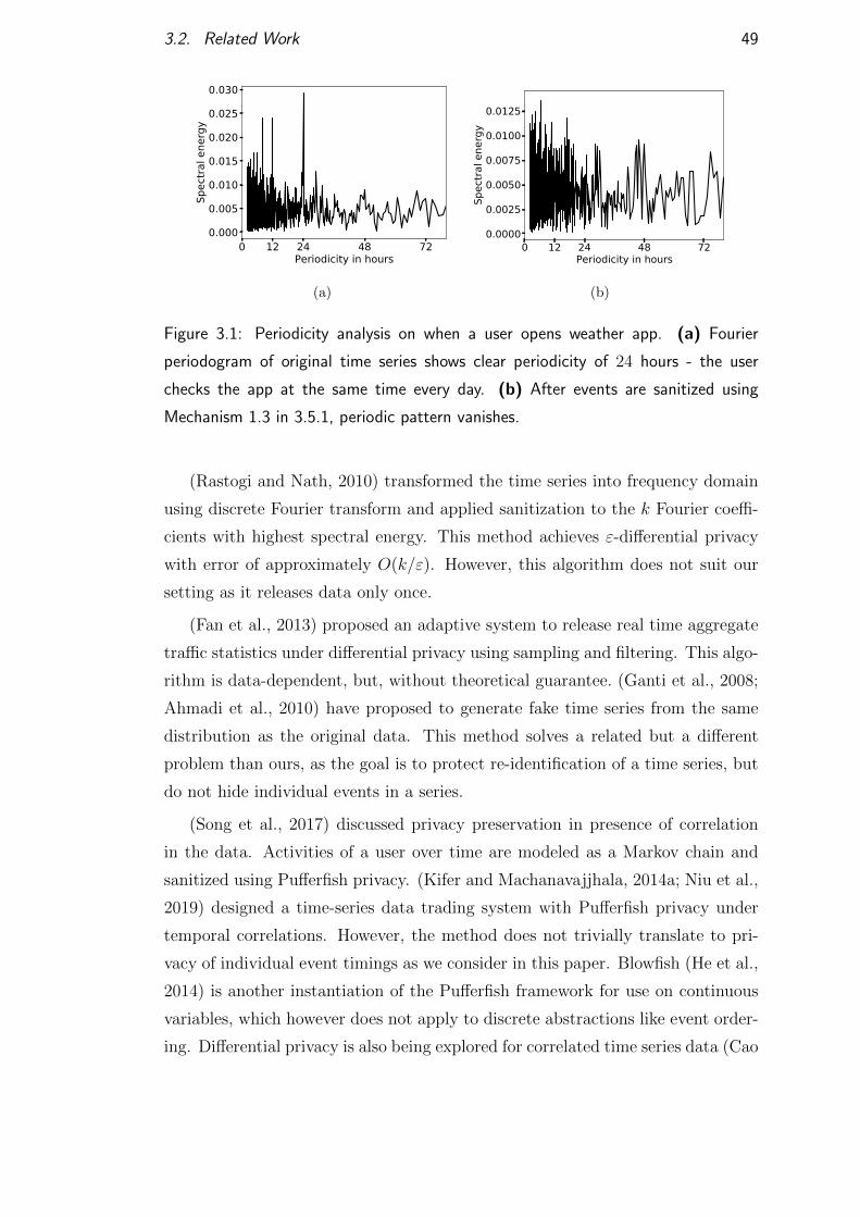
3.2. Related Work 49
0 12 24 48 72Periodicity in hours
0.000
0.005
0.010
0.015
0.020
0.025
0.030
Spec
tral e
nerg
y
0 12 24 48 72Periodicity in hours
0.0000
0.0025
0.0050
0.0075
0.0100
0.0125
Spec
tral e
nerg
y
(a) (b)
Figure 3.1: Periodicity analysis on when a user opens weather app. (a) Fourier
periodogram of original time series shows clear periodicity of 24 hours - the user
checks the app at the same time every day. (b) After events are sanitized using
Mechanism 1.3 in 3.5.1, periodic pattern vanishes.
(Rastogi and Nath, 2010) transformed the time series into frequency domain
using discrete Fourier transform and applied sanitization to the k Fourier coeffi-
cients with highest spectral energy. This method achieves ε-differential privacy
with error of approximately O(k/ε). However, this algorithm does not suit our
setting as it releases data only once.
(Fan et al., 2013) proposed an adaptive system to release real time aggregate
traffic statistics under differential privacy using sampling and filtering. This algo-
rithm is data-dependent, but, without theoretical guarantee. (Ganti et al., 2008;
Ahmadi et al., 2010) have proposed to generate fake time series from the same
distribution as the original data. This method solves a related but a different
problem than ours, as the goal is to protect re-identification of a time series, but
do not hide individual events in a series.
(Song et al., 2017) discussed privacy preservation in presence of correlation
in the data. Activities of a user over time are modeled as a Markov chain and
sanitized using Pufferfish privacy. (Kifer and Machanavajjhala, 2014a; Niu et al.,
2019) designed a time-series data trading system with Pufferfish privacy under
temporal correlations. However, the method does not trivially translate to pri-
vacy of individual event timings as we consider in this paper. Blowfish (He et al.,
2014) is another instantiation of the Pufferfish framework for use on continuous
variables, which however does not apply to discrete abstractions like event order-
ing. Differential privacy is also being explored for correlated time series data (Cao
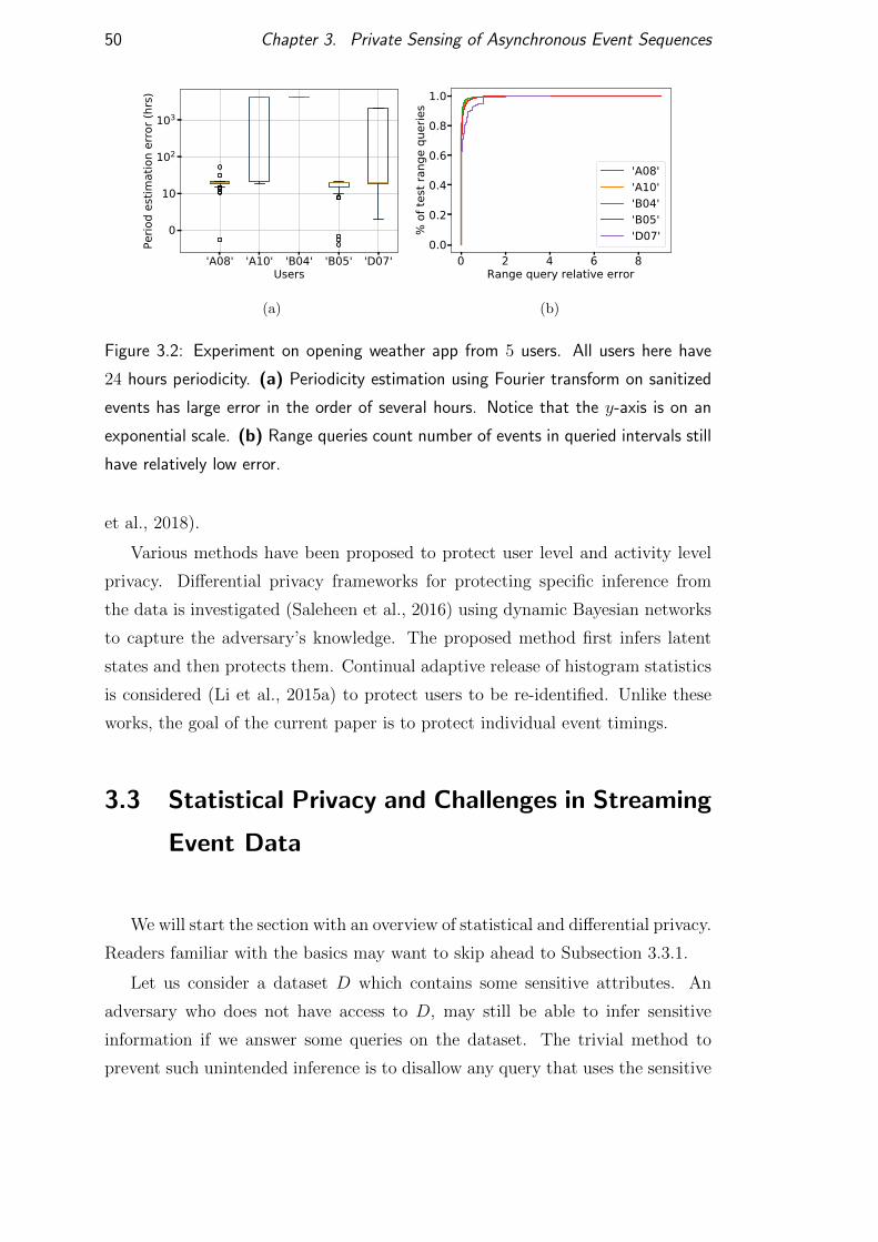
50 Chapter 3. Private Sensing of Asynchronous Event Sequences
'A08' 'A10' 'B04' 'B05' 'D07'Users
0
10
102
103
Perio
d es
timat
ion
erro
r (hr
s)
0 2 4 6 8Range query relative error
0.0
0.2
0.4
0.6
0.8
1.0
% o
f tes
t ran
ge q
uerie
s
'A08''A10''B04''B05''D07'
(a) (b)
Figure 3.2: Experiment on opening weather app from 5 users. All users here have
24 hours periodicity. (a) Periodicity estimation using Fourier transform on sanitized
events has large error in the order of several hours. Notice that the y-axis is on an
exponential scale. (b) Range queries count number of events in queried intervals still
have relatively low error.
et al., 2018).
Various methods have been proposed to protect user level and activity level
privacy. Differential privacy frameworks for protecting specific inference from
the data is investigated (Saleheen et al., 2016) using dynamic Bayesian networks
to capture the adversary’s knowledge. The proposed method first infers latent
states and then protects them. Continual adaptive release of histogram statistics
is considered (Li et al., 2015a) to protect users to be re-identified. Unlike these
works, the goal of the current paper is to protect individual event timings.
3.3 Statistical Privacy and Challenges in Streaming
Event Data
We will start the section with an overview of statistical and differential privacy.
Readers familiar with the basics may want to skip ahead to Subsection 3.3.1.
Let us consider a dataset D which contains some sensitive attributes. An
adversary who does not have access to D, may still be able to infer sensitive
information if we answer some queries on the dataset. The trivial method to
prevent such unintended inference is to disallow any query that uses the sensitive
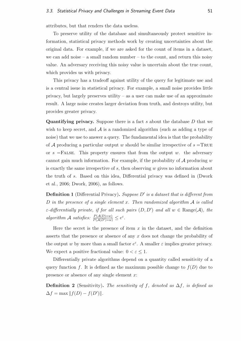
3.3. Statistical Privacy and Challenges in Streaming Event Data 51
attributes, but that renders the data useless.
To preserve utility of the database and simultaneously protect sensitive in-
formation, statistical privacy methods work by creating uncertainties about the
original data. For example, if we are asked for the count of items in a dataset,
we can add noise – a small random number – to the count, and return this noisy
value. An adversary receiving this noisy value is uncertain about the true count,
which provides us with privacy.
This privacy has a tradeoff against utility of the query for legitimate use and
is a central issue in statistical privacy. For example, a small noise provides little
privacy, but largely preserves utility – as a user can make use of an approximate
result. A large noise creates larger deviation from truth, and destroys utility, but
provides greater privacy.
Quantifying privacy. Suppose there is a fact s about the database D that we
wish to keep secret, and A is a randomized algorithm (such as adding a type of
noise) that we use to answer a query. The fundamental idea is that the probability
of A producing a particular output w should be similar irrespective of s =True
or s =False. This property ensures that from the output w. the adversary
cannot gain much information. For example, if the probability of A producing w
is exactly the same irrespective of s, then observing w gives no information about
the truth of s. Based on this idea, Differential privacy was defined in (Dwork
et al., 2006; Dwork, 2006), as follows.
Definition 1 (Differential Privacy). Suppose D′ is a dataset that is different from
D in the presence of a single element x. Then randomized algorithm A is called
ε-differentially private, if for all such pairs (D,D′) and all w ∈ Range(A), the
algorithm A satisfies: P (A(D)=w)P (A(D′)=w)
≤ eε.
Here the secret is the presence of item x in the dataset, and the definition
asserts that the presence or absence of any x does not change the probability of
the output w by more than a small factor eε. A smaller ε implies greater privacy.
We expect a positive fractional value: 0 < ε ≤ 1.
Differentially private algorithms depend on a quantity called sensitivity of a
query function f . It is defined as the maximum possible change to f(D) due to
presence or absence of any single element x:
Definition 2 (Sensitivity). The sensitivity of f , denoted as ∆f , is defined as
∆f = max ‖f(D)− f(D′)‖.
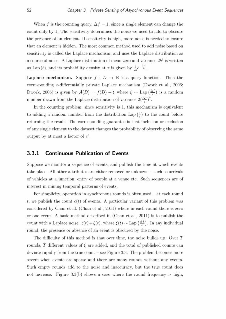
52 Chapter 3. Private Sensing of Asynchronous Event Sequences
When f is the counting query, ∆f = 1, since a single element can change the
count only by 1. The sensitivity determines the noise we need to add to obscure
the presence of an element. If sensitivity is high, more noise is needed to ensure
that an element is hidden. The most common method used to add noise based on
sensitivity is called the Laplace mechanism, and uses the Laplace distribution as
a source of noise. A Laplace distribution of mean zero and variance 2b2 is written
as Lap (b), and its probability density at x is given by 12be−|x|b .
Laplace mechanism. Suppose f : D → R is a query function. Then the
corresponding ε-differentially private Laplace mechanism (Dwork et al., 2006;
Dwork, 2006) is given by A(D) = f(D) + ξ where ξ ∼ Lap(
∆fε
)is a random
number drawn from the Laplace distribution of variance 2(∆fε
)2.
In the counting problem, since sensitivity is 1, this mechanism is equivalent
to adding a random number from the distribution Lap(
1ε
)to the count before
returning the result. The corresponding guarantee is that inclusion or exclusion
of any single element to the dataset changes the probability of observing the same
output by at most a factor of eε.
3.3.1 Continuous Publication of Events
Suppose we monitor a sequence of events, and publish the time at which events
take place. All other attributes are either removed or unknown – such as arrivals
of vehicles at a junction, entry of people at a venue etc. Such sequences are of
interest in mining temporal patterns of events.
For simplicity, operation in synchronous rounds is often used – at each round
t, we publish the count c(t) of events. A particular variant of this problem was
considered by Chan et al. (Chan et al., 2011) where in each round there is zero
or one event. A basic method described in (Chan et al., 2011) is to publish the
count with a Laplace noise: c(t) + ξ(t), where ξ(t) ∼ Lap(
∆fε
). In any individual
round, the presence or absence of an event is obscured by the noise.
The difficulty of this method is that over time, the noise builds up. Over T
rounds, T different values of ξ are added, and the total of published counts can
deviate rapidly from the true count – see Figure 3.3. The problem becomes more
severe when events are sparse and there are many rounds without any events.
Such empty rounds add to the noise and inaccuracy, but the true count does
not increase. Figure 3.3(b) shows a case where the round frequency is high,
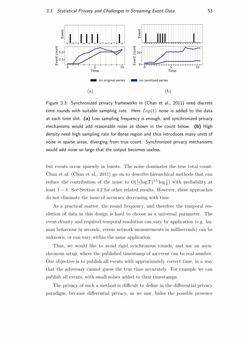
3.3. Statistical Privacy and Challenges in Streaming Event Data 53
Even
t0 5 10
Time
2.5
5.0Ev
ent c
ount
Even
t
0 5 10Time
0
20
Even
t cou
nt
on original series on sanitized series
(a) (b)
Figure 3.3: Synchronized privacy frameworks in (Chan et al., 2011) need discrete
time rounds with suitable sampling rate. Here Lap(1) noise is added to the data
at each time slot. (a) Low sampling frequency is enough, and synchronized privacy
mechanisms would add reasonable noise as shown in the count below. (b) High
density need high sampling rate for dense region and thus introduces many units of
noise in sparse areas, diverging from true count. Synchronized privacy mechanisms
would add noise so large that the output becomes useless.
but events occur sparsely in bursts. The noise dominates the true total count.
Chan et al. (Chan et al., 2011) go on to describe hierarchical methods that can
reduce the contribution of the noise to O(1ε(log T )1.5 log 1
δ) with probability at
least 1− δ. See Section 4.2 for other related results. However, these approaches
do not eliminate the issue of accuracy decreasing with time.
As a practical matter, the round frequency, and therefore the temporal res-
olution of data in this design is hard to choose as a universal parameter. The
event density and required temporal resolution can vary by application (e.g. hu-
man behaviour in seconds, versus network measurements in milliseconds) can be
unknown, or can vary within the same application.
Thus, we would like to avoid rigid synchronous rounds, and use an asyn-
chronous setup, where the published timestamp of an event can be real number.
Our objective is to publish all events with approximately correct time, in a way
that the adversary cannot guess the true time accurately. For example we can
publish all events, with small noises added to their timestamps.
The privacy of such a method is difficult to define in the differential privacy
paradigm, because differential privacy, as we saw, hides the possible presence
54 Chapter 3. Private Sensing of Asynchronous Event Sequences
of an item, not its value. We will resume this discussion in Section 3.4; in the
following subsection, let us introduce Pufferfish privacy, which is a more versatile
framework.
3.3.2 Pufferfish Privacy
The Pufferfish Privacy framework (Kifer and Machanavajjhala, 2014b) allows us
to define any set of facts to be regarded as secret, and protect them probabilisti-
cally. To define the Pufferfish privacy, we first introduce the following sets.
• The set of secrets S to be protected within dataset X ,
• How the secrets shall be protected against each other: by specifying dis-
criminative pairs Q of secrets,
• And the prior knowledge of the adversary, written as a set Θ of prior dis-
tributions, essentially representing how the data is generated.
A discriminative pair can be written as (si, sj) ∈ Q, where si and sj are elements
of S, and represents two facts that we do not want the adversary to be able to
distinguish.
A randomized mechanism M satisfies ε-Pufferfish privacy if for si, sj ∈ S,
(si, sj) ∈ Q, θ ∈ Θ and w ∈ Range(M) the following holds:
e−ε ≤ P (M(X ) = w|si, θ)P (M(X ) = w|sj, θ)
≤ eε (3.1)
assuming P (si|θ) 6= 0 and P (sj|θ) 6= 0. Similar to differential privacy, a smaller
ε implies greater privacy.
The definition is in the Bayesian philosophy. It implies that the truth of si
versus sj does not make a significant difference to the probability of observing
any particular output w. Therefore, when w is in fact observed, the adversary
does not gain any significant certainty whether si or sj is true, compared to what
he already knew based on prior knowledge θ. As we will see in the next section,
the generic nature of secrets and discriminative pairs lets us define privacy for
properties like event ordering and event times.
The interpretation of the prior Θ is that it represents the underlying distribu-
tions generating the data, for example, the vehicle density at a crossing at night,
morning or rush hour, or the distribution of certain events being performed on a
3.4. Model and problem statements 55
mobile phone. Pufferfish allows this distribution to be known to the adversary,
but not true times of actual events.
3.4 Model and problem statements
We want to publish timestamps of events recorded by sensors. We are interested
in publishing data continuously, but not in real time. Events can be assumed to
be published in batches, for example, once in an hour or a day, and taken together
form a stream lasting over long time spans.
The sensors send their data to an aggregator service such as a cloud server,
which then publishes the data. Depending on whether the sensors trust the cloud
server or not, there can be different approaches to publishing.
Labelled and unlabelled event sets. Labelled events are those that carry
IDs or other attributes that can potentially identify events uniquely. Unlabelled
events are those that carry no such attributes or carry the same attributes mak-
ing them indistinguishable. Unlabeled events can occur in various time series
datasets, such as vehicles arriving at a crossing, anonymized access logs of a web
site, etc. Privacy implications of event sets can vary by their label status. Since
we are interested in the timestamp attribute of events, our event sets can be
regarded as unlabeled unless mentioned otherwise.
3.4.1 Sensing Data Collection and Trust Relations
If the devices (or their owners) trust the aggregator and the communication chan-
nel, they can transmit all data to the aggregator, who then sanitizes (privatizes)
and publishes it at suitable time.
If the channel or the aggregator is not trusted, then the devices must take
care of sanitization by themselves. In differential privacy terms, this is called
local privacy (Kasiviswanathan et al., 2011).
All algorithms in this paper can be applied locally, where a device detecting
events can apply sanitization before transmission to the aggregator. This ap-
proach has the advantage that the data transmitted is guaranteed to be private,
since data sanitized by suitable statistical methods are known to be immune to
post processing (Dwork and Roth, 2014). Once the data has been modified by
the mechanism, they carry the privacy guarantee irrespective of how the data is
56 Chapter 3. Private Sensing of Asynchronous Event Sequences
used. This is particularly useful in sensor data that may be shared with various
public and private organisations.
3.4.2 Utility: Range Queries
To ensure that the sanitized data is useful, we measure its utility in terms of
accuracy of range queries. Given a time interval T , the range query asks for the
number of events recorded inside T . The motivation for using range queries as
test of utility is that it is akin to preserving the large scale probability distribution
that generates the data. If the count of events in different ranges is preserved, it
implies that the statistical properties of data are preserved.
3.4.3 Adversary Model and Problem Statements
We assume that the adversary can observe the published events. Note that the
adversary may or may not be able to compromise the communication channel or
aggregator – this is not relevant for us, since we aim to create algorithms with
local privacy. We do, however, assume that the adversary cannot compromise
the distributed devices themselves to observe events as they happen.
As is standard in security and privacy, we assume that the privacy algorithms
and parameters are known to the adversary. However, the random choices – such
as the random numbers generated during an execution are not known.
Under these capabilities of the adversary, we consider the following types
of data protection. More details will be presented in Section 3.5 along with
algorithms.
Problem 1: Protecting the time of a published event. In this problem, we
publish events along with timestamps. However, we do not wish the adversary
to know the true time of the event. Now, in most cases, the adversary does not
need to know the precise number – narrowing the time down to a small interval
of the true time suffices. For example, for human activities like checking into a
venue, accuracy within a few minutes of the true time can be considered accurate
enough.
Thus for an event e at time t, we want to prevent an adversary from gaining
accuracy to within an interval of size ∆ around the true time.
Problem 2: Protecting existence of an event. Suppose we have a sequence

3.5. Privacy mechanisms 57
of unlabeled events, such as arrival of cars at a crossing, or a person’s access to
a website. Such events are known to follow Poisson process models.
Definition 3 (Homogeneous Poisson Process). A homogeneous Poisson process
with intensity λ is one where the number of events X in any unit interval follows
a Poisson distribution:
P (X = K) = e−λ · λK
K!.
The expected value of X is λ. The definition extends naturally to larger
intervals: the number of events in an interval B follows a Poisson distribution of
intensity |B| · λ.
In general, events may not have a uniform rate at all times. Such variable
rates are described by non-homogeneous Poisson processes:
Definition 4 (Non-homogeneous Poisson Process). In a non-homogeneous Pois-
son process defined over an interval A with intensity function λ : A → R≥0, the
number of events X(B) in any subinterval B of the domain follows a Poisson
distribution:
P (X(B) = K) = e−Λ(B) · Λ(B)K
K!,
where Λ(B) =∫Bλ(t) dt is called the mean rate in B.
By using a function λ(t) that may vary in time, the Poisson process can be
used to generate almost any desired distribution of events.
Let us suppose that the adversary suspects the presence of an event inside a
small time interval of size ∆, and wishes to verify that such an event did in fact
take place. Our objective is to prevent such an inference in a statistical privacy
sense.
Problem 3: Protecting Event ordering. Relative ordering of events can
reveal sensitive information. For example, if A leaves a restaurant shortly after
B enters, that reveals that A and B are likely to have met. Thus, in this problem,
we wish to protect the relative ordering of two events that take place within an
interval of size ∆.
3.5 Privacy mechanisms
In this section, we discuss how to achieve statistical privacy of event ei with
respect to any choice of time interval I of size ∆. In some cases the detailed
technical proofs are replaced by their sketches in the interest of space.
58 Chapter 3. Private Sensing of Asynchronous Event Sequences
3.5.1 Problem 1: Protecting Event Times
First we consider that the adversary has the knowledge of a temporal domain
of W , bounded and large, within which an event ei of interest is known to have
taken place.
Let ti be the time of event ei. Assume that ti follows a uniform distribution
over W . This constitutes the prior knowledge θ about the data known to the
adversary. This assumption is for simplicity of analysis – we will discuss later
how the mechanisms work with more general distributions.
The secret we wish to protect here is s : ti ∈ I. The discriminative pair is
(s,¬s). The objective is to obtain ε-Pufferfish privacy for (s,¬s) – thus making
the adversary uncertain between the two possibilities. Note that we are not trying
to obfuscate presence of the event, only its time.
To warm up, let us discuss a trivial mechanism:
Mechanism 1.1: Given an event ei with true time ti, the mechanism outputs
M(ei) = ξ, where ξ is selected uniformly at random in the interval W .
It is easy to argue privacy for this method. Suppose that in a particular run of
the algorithm, M(ei) = w. In this case, P (M(ei)) = w is independent of the truth
of si, therefore, P(M(ei) = w|si, θ
)= P
(M(ei) = w|¬si, θ
), and the mechanism
satisfies 0-Pufferfish privacy. Essentially implying that it adds nothing to the
knowledge of the adversary.
The mechanism is unsatisfactory in the sense of utility. It is in fact completely
independent of the actual value ti – it samples a time from W , which is known,
so it does not add anything to the knowledge of legitimate users either. When
W is large, the perturbation to the event time is large, resulting in poor utility.
Next we consider a mechanism with better utility. Here, we provide the main
results and sketches of the proofs. The detailed proofs are in Section 3.8.
Mechanism 1.2: M outputs M(ei) = ti+ξ, where ξ is selected from the uniform
distribution over [−k∆/2, k∆/2].
This method is more useful since it restricts M(ti) to a smaller interval around
ti. It can be be shown to have ε-Pufferfish privacy for a suitable choice of k.
Theorem 1. Mechanism 1.2 satisfies ε-Pufferfish privacy for k =|W |eε∆
.
The sketch of the proof is that we compute the probability of the output M(ei)
being in [ti − k∆/2, ti + k∆/2], under the respective conditions of si being true
3.5. Privacy mechanisms 59
and ¬si being true. Their ratio can be shown to be bounded by eε, which gives
ε-Pufferfish privacy.
3.5.1.1 Priors of Laplace distribution
Now we relax the requirement for the bounded window W . The adversary’s prior
hypothesis is that the timestamp ti of event ei follows a Laplace distribution
centered at µ, where |µ− ti| ≤ k∆.
Mechanism 1.3: M(ei) = ti + ξ, where ξ ∼ Lap(k∆ε
). That is, a Laplace noise
similar to differential privacy is added.
Theorem 2. A perturbation with Lap(k∆ε
)guarantees ε-Pufferfish privacy.
The proof follows from the definition of Laplace distributions that if the mean
of two Lappace distributions with same variance are separated by distance x,
then at any point their probability densities differ at most by eε. The details is
in Section 3.8.
3.5.2 Problem 2: Protecting event existence in Poisson pro-
cesses
For this problem, we consider Poisson processes with event rate λ in a unit in-
terval. The events are assumed to be unlabeled. Remember that the adversary
wishes to confirm the existence of some event in the interval I of size ∆, where
the adversary has some reason to suspect the presence of an event in I. For
example, this interval may be based on the adversary’s knowledge of external
related events. The adversary also knows the Poisson rate λ.
Let us write ∆ = c/λ. In a Poisson process, the expected interval between
events is 1/λ. If c >> 1 and therefore ∆ >> 1/λ, then there is likely to be
multiple events in I, and presence of an event is not informative for the adversary.
However, when for c ≤ 1 – when the adversary has fairly accurate information
of the event’s possible time, and other events are unlikely in the interval, a small
∆ can isolate the event – it gives the adversary reasonable confidence that any
event in the interval is the one of interest.
In the Pufferfish model, the secret can be defined as s := (∃i : ti ∈ I) –
representing the fact that some event ei has occurred in the small neighborhood
I of size ∆. The discriminative pair is (s,¬s), where ¬s means that no event has

60 Chapter 3. Private Sensing of Asynchronous Event Sequences
taken place in I. For this problem, we describe a mechanism using fake events.
The main intuition is that if we add many fake events to the sequence, then any
interval I is likely to consider events, and thus the presence of events in I does
not give much information to the adversary.
Mechanism 2.1: Introduce a fake event sequence with unit time event rate
Λ = λc
ln eε
(eε−1), and publish both true and fake event times.
The greater rate of this Poisson process ensures that it is likely that one or
more events will be present in the interval, and thus the adversary cannot be
certain of the presence of a true event.
Theorem 3. Fake event rate Λ = λc
ln eε
(eε−1)provides ε-Pufferfish privacy for
existence of events.
Proof. Let η be the situation that an event is seen in I in the stream after adding
fake Poisson events. When s is not true, there is no fake event generated by the
Poisson process. We have P (η | ¬s, θ) = 1 − e−Λ∆. When s is true, η is always
true, thus P (η | s, θ) = 1. When Λ = λc
ln eε
(eε−1), we have P (η|s,θ)
P (η|¬s,θ) ≤ eε.
In this setting, a range query on an interval [x, y] can be answered as follows.
If the total number of events (real and fake) in [x, y] is I, then a range query on
[x, y] is estimated as A(x, y) = n−Λ · (y− x). That is, from the total number of
events in the interval, we subtract the expected number of fake events, to get an
unbiased estimate. The following theorem shows that the error in range counting
introduced by this approach is not large.
Theorem 4. If Λ = λc
ln eε
(eε−1), we get an estimation of the count of real events in
a interval with length L with error bounded by O(√
ΛL log 1β
), with probability
1− β.
This mechanism has the nice property that if each device j applies the mech-
anism with respect to its local Poisson rate λj, then the aggregate global event
stream has the same privacy guarantee with respect to the global Poisson event
rate. This result follows from the Superposition Theorem (Kingman, 1992; Grim-
mett and Stirzaker, 2001) – that the union of Poisson processes is still a Poisson
process.
3.6. Privacy service design and implementation 61
3.5.3 Problem 3: Privacy of event order
Suppose the adversary knows a window W , and knows that events ea and eb
occurred within a short time difference ∆ of each other. The adversary wants to
know if ea occurred before eb or not. So, the secret is sa<b : ta < tb.
Mechanism 3.1: Apply the uniform mechanism (same as in 1.2): M(ei) = ti+ξ,
where ξ is chosen uniformly from [−k∆/2, k∆/2].
Theorem 5. k ≥ 3+eε
eε−1gives ε-Pufferfish privacy with respect to event ordering.
The sketch of the proof considers two cases depending on whether the sanitized
events preserve the order. In each case, it looks at both possibilities of the
secret. To compute probabilities of the form P (M(ta) < M(tb)|sa<b, θ) we need
to consider three regions where the events can be perturbed to, namely [ta −k∆2, tb − k∆
2], [tb − k∆
2, ta + k∆
2], and [ta + k∆
2, tb − k∆
2]. Considering the fact that
the event ordering can only change based on in which region the sanitized events
are placed, we can get the theorem.
This implies that a simple mechanism provides a guarantee against inference of
precise ordering of nearby events. Note that events that are far separated in time
are not covered under this model, since any modified assignment of timestamps
that modifies the ordering of distant events will effectively randomize the the data
completely, destroying all utility.
In Subsections 3.5.1 and 3.5.3 we have used a uniform distribution for simplic-
ity of demonstration. The mechanisms can be easily adapted and implemented
for non-uniform distributions, albeit with a more complex analysis.
3.6 Privacy service design and implementation
To achieve private publishing of data, we designed and implemented a service in
Android. The service accepts raw data from an application, and returns sanitized
data. The same service can of course also be run on a central server to sanitize
data from multiple events. The following discussion applies to both cases. An
application may choose one of the mechanisms described in Section 3.5 to apply
to its data. Along with each event time, it passes the parameters for privacy as
arguments.
The privacy arguments and return values are shown in Table 3.1. We have
presented versions where privacy constraint ε is passed as argument, while the

62 Chapter 3. Private Sensing of Asynchronous Event Sequences
Table 3.1: Callable mechanisms, their arguments and return values in sanitization
service.
Mechanism Arguments Returns
Mechanism 1.2 (ti,∆,W, ε, . . . ) (M(ti), k, . . . )
Mechanism 1.3 (ti,∆, k, ε, . . . ) (M(ti), k, . . . )
Mechanism 2.1 (ti, λ, c, ε, . . . ) (List(ti,Λ, . . . ))
Mechanism 3.1 (ti,∆,W, ε, . . . ) (M(ti), k, . . . )
derived quantity k or Λ are returned along with sanitized values. It is possible
to have versions where the roles of these parameters are switched. In case of
mechanism 2.1, the return value consists of a list of event times instead of a
single time, since this mechanism generates fake events.
The service operates in batch mode, which is more efficient when sanitizing
large number of events. The ellipsis represents that the application can optionally
pass event id or other attributes. The service includes these attributes as is in the
returned set. This feature is useful in research where it is of interest to observe
the sanitized timestamp of an input event. In case of mechanism 3.1, the fake
events carry empty attributes. In case of real usage, it is the responsibility of the
application to remove these attributes before or after the call to the service, or
to set a flag remove labels = True.
Time of event publication. Beyond getting data sanitized by the service, the
application needs to take care in when the timestamp of an event is published,
since in temporal privacy, the time of publication may reveal information about
the true event time. In case of mechanisms 1.2 and 3.1, we recommend publishing
event time stamps after the time window W . In case of mechanism 2.1, events
can be published as soon as real time has passed the timestamp of the event.

3.7. Experiments 63
....Sensing AppPrivacy Config
editorSensing App
Sanitizing Algorithm
Sanitization ServiceStorage Interface
StorageSensing Interface Config Interface
Figure 3.4: System design for sanitization module. The service exposes APIs for san-
itizing events, configuring privacy parameters, and storing configuration parameters.
The design is flexible to have the components be part of a single process or from
different processes.
3.6.1 System design as background Android service
Our implemented service uses Java Apache math library1 for sampling and ran-
domization. The other aspects of the service are shown in Figure 3.4.
Sensing apps. Each app may have different privacy configuration and they can
register and unregister the settings as default.
Privacy configuration editor. Users can view and edit the privacy settings
for various apps.
Persistent storage. The privacy configuration for different apps are stored in
a secure file system.
The sanitization service offers separate interfaces to the sensing apps, privacy
configuration viewer and editor, and storage module. Below are the details of
the interface functions. This is of a proof of concept implementation, and can be
modified as appropriate in different circumstances.
3.7 Experiments
This section describes experiments showing that the privacy preserving mecha-
nisms preserve utility for practical purposes. Highlights of the results are the
following.
1http://commons.apache.org/proper/commons-math/

64 Chapter 3. Private Sensing of Asynchronous Event Sequences
• Sanitized event timings support accurate range queries.
• The proposed methods preserve utility better than competing methods in
terms of range queries.
• Privacy preserving mechanisms work in real event streams of check-ins,
app-usages, and phone unlock events.
3.7.1 Experimental Setup
Datasets. Our experiments use three real world event timing dataset. (i) The
check-in dataset2 consists of 12, 372 check-ins at Akihabara station, Tokyo by
Foursquare users. (ii) Events occur in the app-usage dataset (Shepard et al.,
2011) when a user opens one of his 10 most frequent apps, e.g., SMS, mail,
Facebook, etc. (iii) Event occurs when a user unlocks the phone. Whereas, the
first two datasets contain data for about an year, the last dataset has data of
a week. Further, the last two datasets have data for a single user and the first
dataset include data from 1k users.
Measuring utility. Utility of the sanitized data is measured using range queries.
Each experiment uses 5000 random query ranges and repeated 10 times. If the
range count in the original event stream is n and in the sanitized event stream is
n, then the relative error is ξ = |n−n|n
The relative error is symmetric with respect
to addition, i.e., estimating n+ ∆ and n−∆ incur same error.
3.7.2 Evaluating Event Time Privacy
Figure 3.5(a) and (b) show the distribution of events in the check-in dataset
overlaid in a single day for actual stream and the sanitized stream respectively
using Mechanism 1.3. Visually, the sanitization preserves the critical features in
the distribution, e.g., the peak.
Mechanism 1.2 is evaluatede in Figure 3.5 by varying ε and the error is small
for small values of ε. Figure 3.7(a,b,c) and (d,e,f) evaluate Mechanism 1.3 and
show natural privacy-utility tradeoff by varying ∆ and ε respectively – with in-
creasing ∆ and decreasing ε, privacy increases and the error increases.
2https://www.kaggle.com/chetanism/foursquare-nyc-and-tokyo-checkin-dataset
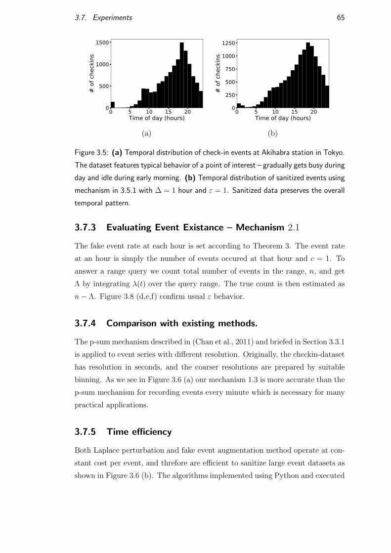
3.7. Experiments 65
0 5 10 15 20Time of day (hours)
0
500
1000
1500
# of
che
ckin
s
0 5 10 15 20Time of day (hours)
0
250
500
750
1000
1250
# of
che
ckin
s
(a) (b)
Figure 3.5: (a) Temporal distribution of check-in events at Akihabra station in Tokyo.
The dataset features typical behavior of a point of interest – gradually gets busy during
day and idle during early morning. (b) Temporal distribution of sanitized events using
mechanism in 3.5.1 with ∆ = 1 hour and ε = 1. Sanitized data preserves the overall
temporal pattern.
3.7.3 Evaluating Event Existance – Mechanism 2.1
The fake event rate at each hour is set according to Theorem 3. The event rate
at an hour is simply the number of events occured at that hour and c = 1. To
answer a range query we count total number of events in the range, n, and get
Λ by integrating λ(t) over the query range. The true count is then estimated as
n− Λ. Figure 3.8 (d,e,f) confirm usual ε behavior.
3.7.4 Comparison with existing methods.
The p-sum mechanism described in (Chan et al., 2011) and briefed in Section 3.3.1
is applied to event series with different resolution. Originally, the checkin-dataset
has resolution in seconds, and the coarser resolutions are prepared by suitable
binning. As we see in Figure 3.6 (a) our mechanism 1.3 is more accurate than the
p-sum mechanism for recording events every minute which is necessary for many
practical applications.
3.7.5 Time efficiency
Both Laplace perturbation and fake event augmentation method operate at con-
stant cost per event, and threfore are efficient to sanitize large event datasets as
shown in Figure 3.6 (b). The algorithms implemented using Python and executed
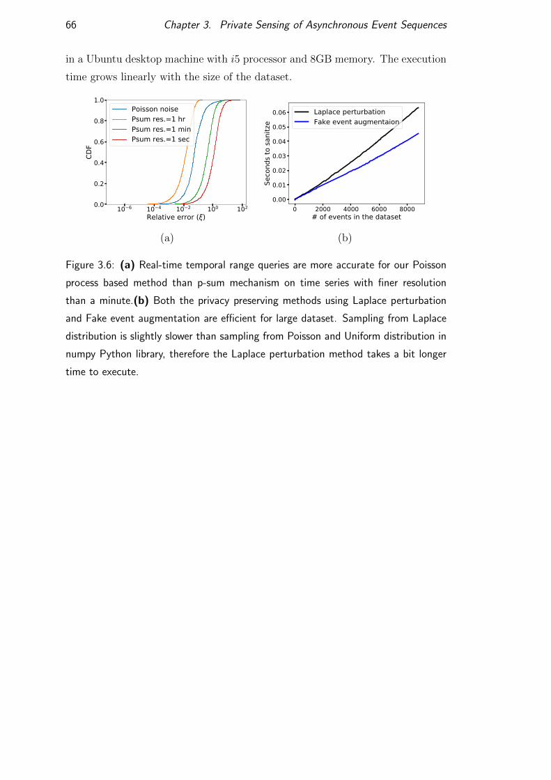
66 Chapter 3. Private Sensing of Asynchronous Event Sequences
in a Ubuntu desktop machine with i5 processor and 8GB memory. The execution
time grows linearly with the size of the dataset.
10 6 10 4 10 2 100 102
Relative error ( )0.0
0.2
0.4
0.6
0.8
1.0CD
F
Poisson noisePsum res.=1 hrPsum res.=1 minPsum res.=1 sec
0 2000 4000 6000 8000# of events in the dataset
0.00
0.01
0.02
0.03
0.04
0.05
0.06
Seco
nds t
o sa
nitz
e
Laplace perturbationFake event augmentaion
(a) (b)
Figure 3.6: (a) Real-time temporal range queries are more accurate for our Poisson
process based method than p-sum mechanism on time series with finer resolution
than a minute.(b) Both the privacy preserving methods using Laplace perturbation
and Fake event augmentation are efficient for large dataset. Sampling from Laplace
distribution is slightly slower than sampling from Poisson and Uniform distribution in
numpy Python library, therefore the Laplace perturbation method takes a bit longer
time to execute.
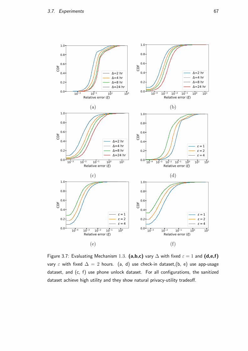
3.7. Experiments 67
10 3 10 1 101 103
Relative error ( )0.0
0.2
0.4
0.6
0.8
1.0
CDF
=2 hr=4 hr=8 hr=24 hr
10 4 10 3 10 2 10 1 100 101
Relative error ( )0.0
0.2
0.4
0.6
0.8
1.0
CDF
=2 hr=4 hr=8 hr=24 hr
(a) (b)
10 3 10 2 10 1 100 101
Relative error ( )0.0
0.2
0.4
0.6
0.8
1.0
CDF
=2 hr=4 hr=8 hr=24 hr
10 4 10 3 10 2 10 1 100 101 102
Relative error ( )0.0
0.2
0.4
0.6
0.8
1.0
CDF
= 1= 2= 4
(c) (d)
10 4 10 3 10 2 10 1 100
Relative error ( )0.0
0.2
0.4
0.6
0.8
1.0
CDF
= 1= 2= 4
10 3 10 2 10 1 100 101
Relative error ( )0.0
0.2
0.4
0.6
0.8
1.0
CDF
= 1= 2= 4
(e) (f)
Figure 3.7: Evaluating Mechanism 1.3. (a,b,c) vary ∆ with fixed ε = 1 and (d,e,f)
vary ε with fixed ∆ = 2 hours. (a, d) use check-in dataset,(b, e) use app-usage
dataset, and (c, f) use phone unlock dataset. For all configurations, the sanitized
dataset achieve high utility and they show natural privacy-utility tradeoff.
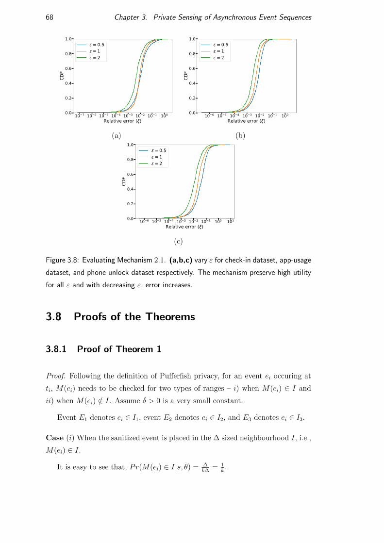
68 Chapter 3. Private Sensing of Asynchronous Event Sequences
10 7 10 6 10 5 10 4 10 3 10 2 10 1 100
Relative error ( )0.0
0.2
0.4
0.6
0.8
1.0
CDF
= 0.5= 1= 2
10 6 10 5 10 4 10 3 10 2 10 1 100
Relative error ( )0.0
0.2
0.4
0.6
0.8
1.0
CDF
= 0.5= 1= 2
(a) (b)
10 6 10 5 10 4 10 3 10 2 10 1 100 101
Relative error ( )0.0
0.2
0.4
0.6
0.8
1.0
CDF
= 0.5= 1= 2
(c)
Figure 3.8: Evaluating Mechanism 2.1. (a,b,c) vary ε for check-in dataset, app-usage
dataset, and phone unlock dataset respectively. The mechanism preserve high utility
for all ε and with decreasing ε, error increases.
3.8 Proofs of the Theorems
3.8.1 Proof of Theorem 1
Proof. Following the definition of Pufferfish privacy, for an event ei occuring at
ti, M(ei) needs to be checked for two types of ranges – i) when M(ei) ∈ I and
ii) when M(ei) /∈ I. Assume δ > 0 is a very small constant.
Event E1 denotes ei ∈ I1, event E2 denotes ei ∈ I2, and E3 denotes ei ∈ I3.
Case (i) When the sanitized event is placed in the ∆ sized neighbourhood I, i.e.,
M(ei) ∈ I.
It is easy to see that, Pr(M(ei) ∈ I|s, θ) = ∆k∆
= 1k.
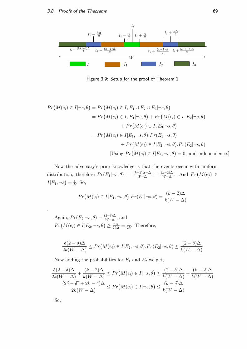
3.8. Proofs of the Theorems 69
Figure 3.9: Setup for the proof of Theorem 1
Pr(M(ei) ∈ I|¬s, θ
)= Pr
(M(ei) ∈ I, E1 ∪ E2 ∪ E3|¬s, θ
)= Pr
(M(ei) ∈ I, E1|¬s, θ
)+ Pr
(M(ei) ∈ I, E2|¬s, θ
)+ Pr
(M(ei) ∈ I, E3|¬s, θ
)= Pr
(M(ei) ∈ I|E1,¬s, θ
).P r(E1|¬s, θ)
+ Pr(M(ei) ∈ I|E2,¬s, θ
).P r(E2|¬s, θ)
[Using Pr(M(ei) ∈ I|E3,¬s, θ
)= 0, and independence.]
Now the adversary’s prior knowledge is that the events occur with uniform
distribution, therefore Pr(E1|¬s, θ) = (k−1)∆−∆W−∆
= (k−2)∆W−∆
. And Pr(M(ej) ∈
I|E1,¬s)
= 1k. So,
Pr(M(ei) ∈ I|E1,¬s, θ
).P r(E1|¬s, θ) =
(k − 2)∆
k(W −∆)
.
Again, Pr(E2|¬s, θ) = (2−δ)∆W−∆
, and
Pr(M(ei) ∈ I|E2,¬s, θ
)≥ δ∆
2k∆= δ
2k. Therefore,
δ(2− δ)∆2k(W −∆)
≤ Pr(M(ei) ∈ I|E2,¬s, θ
).P r(E2|¬s, θ) ≤
(2− δ)∆k(W −∆)
Now adding the probabilities for E1 and E2 we get,
δ(2− δ)∆2k(W −∆)
+(k − 2)∆
k(W −∆)≤ Pr
(M(ei) ∈ I|¬s, θ
)≤ (2− δ)∆k(W −∆)
+(k − 2)∆
k(W −∆)
(2δ − δ2 + 2k − 4)∆
2k(W −∆)≤ Pr
(M(ei) ∈ I|¬s, θ
)≤ (k − δ)∆k(W −∆)
So,

70 Chapter 3. Private Sensing of Asynchronous Event Sequences
(W −∆)
(k − δ)∆≤
Pr(M(ei) ∈ I|s, θ
)Pr(M(ei) ∈ I|¬s, θ
) ≤ 2(W −∆)
(2δ − δ2 + 2k − 4)∆(3.2)
Case (ii) When the sanitized event is placed in the ∆ sized neighbourhood N ,
i.e., M(ei) /∈ I.
It is easy to see that, Pr(M(ei) /∈ I|s, θ) = k−1k
. Again, similar to the above
case,
Pr(M(ei) /∈ I|¬s, θ
)= Pr
(M(ei) ∈ I, E1 ∪ E2|¬s, θ
)+ Pr
(M(ei) /∈ I, E3|¬s, θ
)Now, Pr(E1 ∪ E2|¬s, θ) = ∆(k−δ)
W−∆.
Again, k−1k≤ Pr
(M(ei) /∈ I, E1 ∪ E2|¬s, θ
)≤ k−δ
k, therefore,
(k − 1)(k − δ)k(W −∆)
≤ Pr(M(ei) /∈ I, E1 ∪ E2|¬s, θ
)≤ (k − δ)2∆
k(W −∆)
It is easy to see that, Pr(M(ei) ∈ I|E3,¬s, θ
)= 1. Now, Pr(E3|¬s) =
W−(k+1−δ)∆W−∆
. Therefore, Pr(M(ei) ∈ I, E3, |¬s, θ
)= W−(k+1−δ)∆
W−∆. Hence, we get
the following,
(k − 1)(k − δ)k(W −∆)
+W − (k + 1− δ)∆
W −∆≤ Pr
(M(ei) /∈ I|¬s, θ
)≤ (k − δ)2∆
k(W −∆)
Or,(k − 1)(k − δ) +Wk − k∆(k + 1− δ)
k(W −∆)
≤ Pr(M(ei) /∈ I|¬s, θ
)≤ Wk + δ2∆− k∆(1 + δ)
k(W −∆)
Combining the results for E1 ∪ E2 and E3, we get,
(W −∆)
(k − 1)(Wk + δ2∆− k∆(1 + δ))≤
Pr(M(ei) /∈ I|s, θ
)Pr(M(ei) /∈ I|¬s, θ
) ≤(W −∆)
(k − 1)[(k − 1)(k − δ) +Wk − k∆(k + 1− δ)](3.3)
Combining the lower bound of Equation 3.2 and Equation 3.3 we get.

3.8. Proofs of the Theorems 71
min
((W −∆)
(k − δ)∆,
(W −∆)
(k − 1)(Wk + δ2∆− k∆(1 + δ))
)≤
Pr(M(ei) = w|s, θ
)Pr(M(ei) = w|¬s, θ
) ≤max
(2(W −∆)
(2δ − δ2 + 2k − 4)∆,
(W −∆)
(k − 1)[(k − 1)(k − δ) +Wk − k∆(k + 1− δ)]
)Or,
∆
2Wk2≤
Pr(M(ei) = w|s, θ
)Pr(M(ei) = w|¬s, θ
) ≤ 2W
k∆when W ≥ 2∆
Or, eε ≥ 2W
k∆and e−ε ≤ ∆
2Wk2[from Pufferfish privacy defination.]
Or, k ≥ 2W
eε∆
3.8.2 Proof of Theorem 2
Proof. Similar to the above proof, for an event ei occuring at ti, M(ei) needs to
be checked for two types of ranges – i) when M(ei) ∈ I and ii) when M(ei) /∈ I.
Case (i) When the sanitized event is placed in the ∆ sized neighbourhood I, i.e.,
M(ei) ∈ I.
∆∫0
Lap(x; 0, b)dx ≤ Pr(M(ei) ∈ I|s, θ) ≤∆/2∫
−∆/2
Lap(x; 0, b)dx
Or, −1
2
[e−x/b
]∆
0
≤ Pr(M(ei) ∈ I|s, θ) ≤ 2.
∆/2∫0
Lap(x; 0, b)dx
Or,1
2[1− e−∆/b] ≤ Pr(M(ei) ∈ I|s, θ) ≤
[e−x/b
]∆/2
0
Or,1
2[1− e−∆/b] ≤ Pr(M(ei) ∈ I|s, θ) ≤ (1− e−∆/(2b)) (3.4)
Now, for the secret ¬s, when event ei does not occur in I,
K∆∫k∆−∆
Lap(x; 0, b)dx ≤ Pr(M(ei) ∈ I|¬s, θ) ≤∆∫
0
Lap(x; 0, b)dx
Or,e−k∆/b
2(e∆/b − 1) ≤ Pr(M(ei) ∈ I|¬s, θ) ≤
1
2(1− e−∆/b) (3.5)
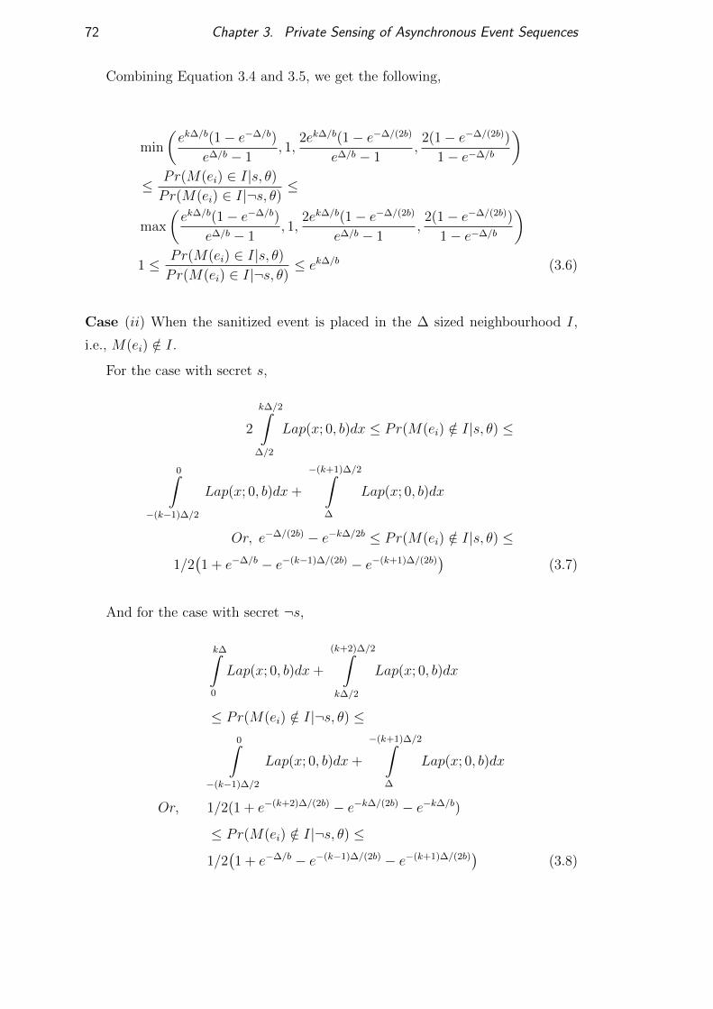
72 Chapter 3. Private Sensing of Asynchronous Event Sequences
Combining Equation 3.4 and 3.5, we get the following,
min
(ek∆/b(1− e−∆/b)
e∆/b − 1, 1,
2ek∆/b(1− e−∆/(2b)
e∆/b − 1,2(1− e−∆/(2b))
1− e−∆/b
)≤ Pr(M(ei) ∈ I|s, θ)Pr(M(ei) ∈ I|¬s, θ)
≤
max
(ek∆/b(1− e−∆/b)
e∆/b − 1, 1,
2ek∆/b(1− e−∆/(2b)
e∆/b − 1,2(1− e−∆/(2b))
1− e−∆/b
)1 ≤ Pr(M(ei) ∈ I|s, θ)
Pr(M(ei) ∈ I|¬s, θ)≤ ek∆/b (3.6)
Case (ii) When the sanitized event is placed in the ∆ sized neighbourhood I,
i.e., M(ei) /∈ I.
For the case with secret s,
2
k∆/2∫∆/2
Lap(x; 0, b)dx ≤ Pr(M(ei) /∈ I|s, θ) ≤
0∫−(k−1)∆/2
Lap(x; 0, b)dx+
−(k+1)∆/2∫∆
Lap(x; 0, b)dx
Or, e−∆/(2b) − e−k∆/2b ≤ Pr(M(ei) /∈ I|s, θ) ≤
1/2(1 + e−∆/b − e−(k−1)∆/(2b) − e−(k+1)∆/(2b)
)(3.7)
And for the case with secret ¬s,
k∆∫0
Lap(x; 0, b)dx+
(k+2)∆/2∫k∆/2
Lap(x; 0, b)dx
≤ Pr(M(ei) /∈ I|¬s, θ) ≤0∫
−(k−1)∆/2
Lap(x; 0, b)dx+
−(k+1)∆/2∫∆
Lap(x; 0, b)dx
Or, 1/2(1 + e−(k+2)∆/(2b) − e−k∆/(2b) − e−k∆/b)
≤ Pr(M(ei) /∈ I|¬s, θ) ≤
1/2(1 + e−∆/b − e−(k−1)∆/(2b) − e−(k+1)∆/(2b)
)(3.8)

3.8. Proofs of the Theorems 73
Now the ratio of Equation 3.7 and 3.8 is bounded by the following.
e−∆/(2b) − e−k∆/2b
1/2(1 + e−∆/b − e−(k−1)∆/(2b) − e−(k+1)∆/(2b)
)≤ Pr(M(ei) /∈ I|s, θ)Pr(M(ei) /∈ I|¬s, θ)
≤ 1
Or, e−k∆/b ≤ Pr(M(ei) /∈ I|s, θ)Pr(M(ei) /∈ I|¬s, θ)
≤ 1 (3.9)
Finally we combine Equation 3.6 and 3.9 and get the following.
e−k∆/b ≤ Pr(M(ei) = w|s, θ)Pr(M(ei) = w|¬s, θ)
≤ e(k−1)∆/b
From the Pufferfish privacy definition,
e−ε ≤ e−k∆/b ≤ Pr(M(ei) = w|s, θ)Pr(M(ei) = w|¬s, θ)
≤ e(k−1)∆/b ≤ eε
Which gives the bound b ≥ k∆ε
.
3.8.3 Proof of Theorem 4
To proof the theorem we need the following lemma first.
Lemma 1. Goldreich (2017) If a random variable Y follows a Poisson distribu-
tion with mean ΛY , P (|Y − ΛY | ≥ α) ≤ 2 exp(− α2
2(ΛY +α)
).
Proof. Given a interval [x, y] with length L, denote the count of real events as
n∗. A(x, y) − n∗ = n − n∗ − Λ · (y − x). Notice that n − n∗ is the count of fake
events, following the Poisson with mean Λ · (y − x). Applying the Lemma 1, for
any β, we set α ≥ log 2β
+√
log2 2β
+ 2Λ log 2β, and we have
P
(|A(x, y)− n∗| ≤ log
2
β+
√log2 2
β+ 2Λ log
2
β
)≥ 1− β.
Rearranging, we get the theorem.
3.8.4 Proof of Theorem 5
Proof. For simplicity of calculation let us assume ∆ = 1 (we can scale everything
to make this happen). Form the figure, |I2| = (k − 1). For two events ea and eb

74 Chapter 3. Private Sensing of Asynchronous Event Sequences
Figure 3.10: Setup for the proof of Theorem 5
occuring at time ta, tb, the situation E denotes that the fact that M(ea) ≤M(eb),
and ¬E denotes the complement of this situation. Therefore,
Pr(E|s, θ) ≤Pr(M(ea) ∈ I1) + Pr(M(ta) ∈ I3)
+ Pr(M(ea) ≤M(tb),M(ea) ∈ I2,M(eb) ∈ I2)
Or, ≤2
k+
(k − 1)2
k2
(k − 1) + 1
2(k − 1)
≤2
k+k − 1
2k
≤k + 3
2k(3.10)
For the lower bound we have ta and tb almost coencide, which makes the
R3 ≈ k,
Pr(E|s, θ) ≥k + 1
2k(3.11)
Now, combining Equation 3.11 and equation 3.10, we have the following.
k + 1
2k≤ Pr(E|s, θ) ≤ k + 3
2k(3.12)
Again for the secret ¬s, we have the following.
(k − 1)2
k2
k − 1 + 1
2(k − 1)≤Pr(E|¬s, θ) ≤ k + 1
2k
Or,k − 1
2k≤Pr(E|¬s, θ) ≤ k + 1
2k(3.13)
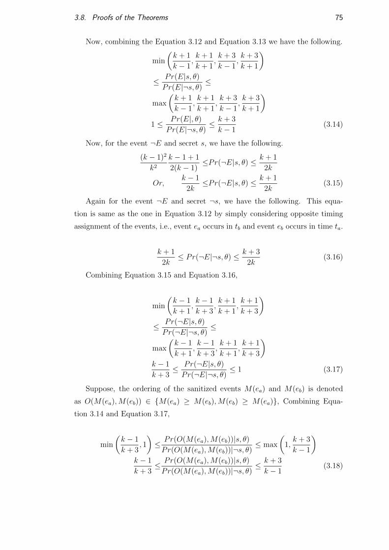
3.8. Proofs of the Theorems 75
Now, combining the Equation 3.12 and Equation 3.13 we have the following.
min
(k + 1
k − 1,k + 1
k + 1,k + 3
k − 1,k + 3
k + 1
)≤ Pr(E|s, θ)Pr(E|¬s, θ)
≤
max
(k + 1
k − 1,k + 1
k + 1,k + 3
k − 1,k + 3
k + 1
)1 ≤ Pr(E|, θ)
Pr(E|¬s, θ)≤ k + 3
k − 1(3.14)
Now, for the event ¬E and secret s, we have the following.
(k − 1)2
k2
k − 1 + 1
2(k − 1)≤Pr(¬E|s, θ) ≤ k + 1
2k
Or,k − 1
2k≤Pr(¬E|s, θ) ≤ k + 1
2k(3.15)
Again for the event ¬E and secret ¬s, we have the following. This equa-
tion is same as the one in Equation 3.12 by simply considering opposite timing
assignment of the events, i.e., event ea occurs in tb and event eb occurs in time ta.
k + 1
2k≤ Pr(¬E|¬s, θ) ≤ k + 3
2k(3.16)
Combining Equation 3.15 and Equation 3.16,
min
(k − 1
k + 1,k − 1
k + 3,k + 1
k + 1,k + 1
k + 3
)≤ Pr(¬E|s, θ)Pr(¬E|¬s, θ)
≤
max
(k − 1
k + 1,k − 1
k + 3,k + 1
k + 1,k + 1
k + 3
)k − 1
k + 3≤ Pr(¬E|s, θ)Pr(¬E|¬s, θ)
≤ 1 (3.17)
Suppose, the ordering of the sanitized events M(ea) and M(eb) is denoted
as O(M(ea),M(eb)) ∈ {M(ea) ≥ M(eb),M(eb) ≥ M(ea)}, Combining Equa-
tion 3.14 and Equation 3.17,
min
(k − 1
k + 3, 1
)≤ Pr(O(M(ea),M(eb))|s, θ)Pr(O(M(ea),M(eb))|¬s, θ)
≤ max
(1,k + 3
k − 1
)k − 1
k + 3≤ Pr(O(M(ea),M(eb))|s, θ)Pr(O(M(ea),M(eb))|¬s, θ)
≤ k + 3
k − 1(3.18)

76 Chapter 3. Private Sensing of Asynchronous Event Sequences
For ε-Pufferfish privacy we have k+3k−1≤ eε, which gives k ≥ 3+eε
eε−1.

Part II
Learning from Spatial Data
77


Chapter 4
Topological Signatures For Fast
Mobility Analysis
Analytic methods can be difficult to build and costly to train for mobility data.
We show that information about the topology of the space and how mobile objects
navigate the obstacles can be used to extract insights about mobility at larger
distance scales. The main contribution of this chapter is a topological signature
that maps each trajectory to a relatively low dimensional Euclidean space, so
that now they are amenable to standard analytic techniques. Data mining tasks:
nearest neighbor search with locality sensitive hashing, clustering, regression, etc.,
work more efficiently in this signature space. We define the problem of mobility
prediction at different distance scales, and show that with the signatures simple
k nearest neighbor based regression perform accurate prediction. Experiments
on multiple real datasets show that the framework using topological signatures
is accurate on all tasks, and substantially more efficient than machine learning
applied to raw data. Theoretical results show that the signatures contain enough
topological information to reconstruct non-self-intersecting trajectories upto ho-
motopy type. The construction of signatures is based on a differential form that
can be generated in a distributed setting using local communication, and a sig-
nature can be locally and inexpensively updated and communicated by a mobile
agent.
79
80 Chapter 4. Topological Signatures For Fast Mobility Analysis
4.1 Introduction
Location traces are computationally challenging to process. Distances between
trajectories like Frechet and Hausdorff distances (Alt and Godau, 1995) do not
form a normed space, Dynamic time warping distance (Sakoe and Chiba, 1978)
does not even form a metric (Driemel and Silvestri, 2017). As a result, typical
computational methods are difficult to apply. Specialized techniques have been
developed for location traces. Theoretical approaches such as locality sensitive
hashing have to be tailored to trajectories for faster near neighbor search (Indyk,
2002; Driemel and Silvestri, 2017; Astefanoaei et al., 2018); computation of me-
dians (Buchin et al., 2013), popular paths (Katsikouli et al., 2018) etc have also
been considered.
Analysis and prediction of motion have been developed with Markov mod-
els (Xue et al., 2013; Ziebart et al., 2008; Liu et al., 1998) that assume motion
to depend only on the current “state” of an agent and not on longer history.
However, recent experimental results show that the memoryless assumption of
Markov models does not hold in real location data, since agents do not execute a
random walk, but move with the purpose to reach a destination (Srivatsa et al.,
2013). Specialized neural network based models (Wu et al., 2017; Lv et al., 2018)
with the power to encode longer history are shown in practice to be effective for
next road segment prediction, although they do not provide rigorous models for
other general tasks, e.g., search and comparison of trajectories. We instead seek
a framework for interpretable encoding of large scale properties of trajectories,
that is compatible with a range of analytic methods.
The motion of objects is determined by the major obstacles in the plane,
which defines the geometry and topology of the space. However, considerations of
topology raise complex issues, and traditional quantities like Frechet distance are
prohibitively expensive to compute in domains with obstacles (Chambers et al.,
2010). Geometric algorithms thus usually assume motion in a simple plane, or of
same topological type.
In past work, Hodge theory and relative homology from algebraic topology
have been used for the purpose of topological classification (Yin et al., 2015;
Pokorny et al., 2016). However, these approaches are only applicable to specific
start and end points of trajectories, and yield only discrete classifications by
homotopy type, which is not general enough for use in further analysis. They are
4.1. Introduction 81
also expensive to compute. We intend to overcome these obstacles by using more
flexible topological constructs.
Our contributions. This chapter shows that topological information can en-
hance mobility analysis by meaningfully encoding large scale patterns of move-
ment, and demonstrates how the relevant information can be represented com-
pactly.
The geometry and topology of the space of mobility itself can be discretized
as a graph, where regions of zero or little activity are treated as obstacles or holes,
and the remaining space is triangulated based on a suitable set of vertices.
Let us define a discrete differential form ξ : E → R as a function that assigns
values to directed edges. For any directed edge ab, the function ξ satisfies ξ(ab) =
−ξ(ba), that is, the values on an edge and its reverse are negations of each other
(See Section 4.3). Further, the values on the edges sum to zero around any face
of the graph, except possibly the obstacles. For each obstacle i, we define a
differential form ξi such that around obstacle i, ξi on the edges sum to 1, and
thus preserves topological information with respect to this obstacle.
For any mobility trace A, the differential form values along its directed edges
are added to obtain ξi(A). For a trajectory that goes around an obstacle i, ξi(A) =
1. In a space with k obstacles, the general differential form ξ = {ξ1, ξ2, . . . ξk} is
a vector of length k.
The significant property here is that a signature element ξi(A) can have a real
numbered value when A is not a perfect loop. The signature ξ(A) ∈ Rk is a point
in k dimensional space. Thus, beyond simple topological equality, the signatures
can represent topological similarity. The mapping to a normed space enables
standard analytic techniques like clustering, regression, density estimation, etc.
We discuss the basic construction in Section 4.4 and the detailed technique in
Section 4.5.
Summations over differential forms preserve only large scale properties, and
are insensitive to noise that does not change topological type of a trajectory.
As a result, the signatures are invariant to localization errors and GPS noise.
They are compact compared to real trajectory data, and can be easily exchanged
between mobile nodes to perform mobility comparison among nearby nodes. It
is efficient to compute and to update incrementally as an object moves in the
plane. Comparison between trajectories is now reduced to comparison of points
in a low dimensional space. The signature of a simple trajectory contains sufficient
82 Chapter 4. Topological Signatures For Fast Mobility Analysis
information to provably reconstruct it upto homotopy equivalence.
The knowledge of global topological behaviors of trajectories can be used to
make predictions at larger scale beyond the next road segment. For this purpose,
we define a notion of prediction at an arbitrary scale r. Motion prediction on
larger scale can be useful in many applcations, e.g., to predict tourists visiting var-
ious attractions in a city. Simple k nearest neighbor regression on the signatures
performs comparably to expensive and opaque neural network based methods,
which suggests that the topological features are essential to understanding and
prediction of motion.
Data mining techniques of locality sensitive hashing, dimension reduction,
etc run efficiently and accurately on the signatures (Section 4.6). Experiments
(Section 4.7) show that the dimensionality of the signatures can be reduced by
selecting only a few obstacles from the domain, and this further increases the
efficiency of the system. Based on how the trajectories traverse the domains, the
obstacles themselves can be characterized by how they influence mobility.
Section 4.2 discusses some related works and how the new approach compares
with them.
Before we move on with technical details, let us summarize our approach into
the following steps: 1. Find obstacle as sparse regions of the plane 2. construct a
differential 1-form for each obstacle. 3. As a mobile agent moves, use these forms
to track how it circumnavigates each obstacle and get a point in Euclidean space,
where each dimension represents behavior with respect to one obstacle. 4. Apply
efficient analytic techniques treating trajectories as points in Euclidean space.
4.2 Related work
Hodge decomposition of a randomly generated vector field has been used in (Yin
et al., 2015) to classify paths into homotopy types. This approach relies on
a numerical process, and only applies to trajectories with same start and end
points. This problem is avoided to an extent in (Pokorny et al., 2016), which
uses relative homology, and marks certain regions of the space where start and
end points lie, but other trajectories do not pass. Thus these approaches do not
apply to general trajectory datasets of the type we have considered here. Both
these methods are also computationally expensive.
In other works, topological characterization has been used to measure dis-
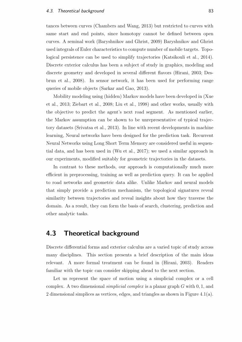
4.3. Theoretical background 83
tances between curves (Chambers and Wang, 2013) but restricted to curves with
same start and end points, since homotopy cannot be defined between open
curves. A seminal work (Baryshnikov and Ghrist, 2009) Baryshnikov and Ghrist
used integrals of Euler characteristics to compute number of mobile targets. Topo-
logical persistence can be used to simplify trajectories (Katsikouli et al., 2014).
Discrete exterior calculus has been a subject of study in graphics, modeling and
discrete geometry and developed in several different flavors (Hirani, 2003; Des-
brun et al., 2008). In sensor network, it has been used for performing range
queries of mobile objects (Sarkar and Gao, 2013).
Mobility modeling using (hidden) Markov models have been developed in (Xue
et al., 2013; Ziebart et al., 2008; Liu et al., 1998) and other works, usually with
the objective to predict the agent’s next road segment. As mentioned earlier,
the Markov assumption can be shown to be unrepresentative of typical trajec-
tory datasets (Srivatsa et al., 2013). In line with recent developments in machine
learning, Neural networks have been designed for the prediction task. Recurrent
Neural Networks using Long Short Term Memory are considered useful in sequen-
tial data, and has been used in (Wu et al., 2017); we used a similar approach in
our experiments, modified suitably for geometric trajectories in the datasets.
In contrast to these methods, our approach is computationally much more
efficient in preprocessing, training as well as prediction query. It can be applied
to road networks and geometric data alike. Unlike Markov and neural models
that simply provide a prediction mechanism, the topological signatures reveal
similarity between trajectories and reveal insights about how they traverse the
domain. As a result, they can form the basis of search, clustering, prediction and
other analytic tasks.
4.3 Theoretical background
Discrete differential forms and exterior calculus are a varied topic of study across
many disciplines. This section presents a brief description of the main ideas
relevant. A more formal treatment can be found in (Hirani, 2003). Readers
familiar with the topic can consider skipping ahead to the next section.
Let us represent the space of motion using a simplicial complex or a cell
complex. A two dimensional simplicial complex is a planar graph G with 0, 1, and
2 dimensional simplices as vertices, edges, and triangles as shown in Figure 4.1(a).
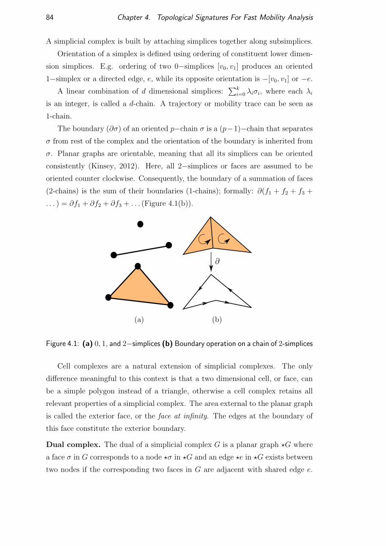
84 Chapter 4. Topological Signatures For Fast Mobility Analysis
A simplicial complex is built by attaching simplices together along subsimplices.
Orientation of a simplex is defined using ordering of constituent lower dimen-
sion simplices. E.g. ordering of two 0−simplices [v0, v1] produces an oriented
1−simplex or a directed edge, e, while its opposite orientation is −[v0, v1] or −e.A linear combination of d dimensional simplices:
∑ki=0 λiσi, where each λi
is an integer, is called a d-chain. A trajectory or mobility trace can be seen as
1-chain.
The boundary (∂σ) of an oriented p−chain σ is a (p−1)−chain that separates
σ from rest of the complex and the orientation of the boundary is inherited from
σ. Planar graphs are orientable, meaning that all its simplices can be oriented
consistently (Kinsey, 2012). Here, all 2−simplices or faces are assumed to be
oriented counter clockwise. Consequently, the boundary of a summation of faces
(2-chains) is the sum of their boundaries (1-chains); formally: ∂(f1 + f2 + f3 +
. . . ) = ∂f1 + ∂f2 + ∂f3 + . . . (Figure 4.1(b)).
(a) (b)
Figure 4.1: (a) 0, 1, and 2−simplices (b) Boundary operation on a chain of 2-simplices
Cell complexes are a natural extension of simplicial complexes. The only
difference meaningful to this context is that a two dimensional cell, or face, can
be a simple polygon instead of a triangle, otherwise a cell complex retains all
relevant properties of a simplicial complex. The area external to the planar graph
is called the exterior face, or the face at infinity. The edges at the boundary of
this face constitute the exterior boundary.
Dual complex. The dual of a simplicial complex G is a planar graph ?G where
a face σ in G corresponds to a node ?σ in ?G and an edge ?e in ?G exists between
two nodes if the corresponding two faces in G are adjacent with shared edge e.

4.4. Topological signatures 85
An example is shown in Figure 4.2(a).
4.3.1 Discrete differential 1-forms and co-chains
Differential forms are defined as functions over the directed cells of the cell com-
plex. Specifically, 1-forms are values for the edge set E of a graph as ω : E → R.
The values are associated with directed edges, so that ω(ab) = −ω(ba). Given a
discrete trace written as e1 + e2 + e3 . . . , the integral of the form over it is now
computed as sum of ω over the directed edges: ω(e1) + ω(e2) + ω(e3) . . . .
The function ω thus defines a co-chain in C1(G;R) that maps 1-chains to real
values. The entire construct translates to a dual with a dual function ?ω defined
simply as ?ω(?e) = ω(e). Thus ?ω, yields a differential form ω, which will be
useful in the following section.
Sources and sinks. Suppose X(v) is the set of edges of the type (v, ◦) – that
is, all edges incident on v, with orientation selected as pointing outward from v.
Then we can compute the net outflow from v as h(v) =∑e∈X(v)
ω(e). Depending
on this value, v can be a:
• Source: net outflow h(v) > 0.
• Internal or regular node: net outflow h(v) = 0.
• Sink: net outflow h(v) < 0.
Observe the effect on the dual system. For a primal face f with dual vertex
?f , we have :∑
?e∈X(?f)
?ω(?e) = ω(∂f).
4.4 Topological signatures
The goal is to utilize differential forms to characterize the behavior of the traces
with respect to obstacles in the domain. We assume that the obstacles such as
buildings and lakes reside in the larger faces of the graph and the mobile objects
move along the nodes and edges of the graph. The question of what constitutes
important obstacles in a domain will be taken up later, for now assume that some
faces are given to us to be treated as obstacles.
Dual sources. Each obstacle is a source of a dual vector field ?ξ. More specifi-
cally, given a face f with an obstacle, the corresponding dual node ?f is the only
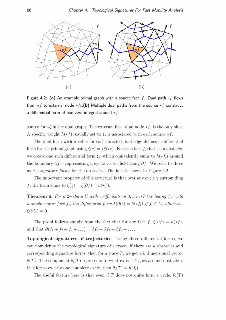
86 Chapter 4. Topological Signatures For Fast Mobility Analysis
(a) (b)
Figure 4.2: (a) An example primal graph with a source face f . Dual path ?ρ flows
from ?f to external node ?f0.(b) Multiple dual paths from the source ?f construct
a differential form of non-zero integral around ?f .
source for ?ξ in the dual graph. The external face, dual node ?f0 is the only sink.
A specific weight h(?f), usually set to 1, is associated with each source ?f .
The dual form with a value for each directed dual edge defines a differential
form for the primal graph using ξ(e) = ?ξ(?e). For each face fi that is an obstacle,
we create one such differential form ξi, which equivalently sums to h(?fi) around
the boundary ∂f – representing a cyclic vector field along ∂f . We refer to these
as the signature forms for the obstacles. The idea is shown in Figure 4.2.
The important property of this structure is that over any cycle γ surrounding
f , the form sums to ξ(γ) = ξ(∂f) = h(?f).
Theorem 6. For a 2−chain U with coefficients in 0, 1 in G (excluding f0) with
a single source face fi, the differential form ξ(∂U) = h(?fi) if fi ∈ U , otherwise
ξ(∂U) = 0.
The proof follows simply from the fact that for any face f , ξ(∂f) = h(?f),
and that ∂(f1 + f2 + f3 + . . . ) = ∂f1 + ∂f2 + ∂f3 + . . . .
Topological signatures of trajectories. Using these differential forms, we
can now define the topological signature of a trace. If there are k obstacles and
corresponding signature forms, then for a trace T , we get a k dimensional vector
θ(T ). The component θi(T ) represents to what extent T goes around obstacle i.
If it forms exactly one complete cycle, then θi(T ) = h(fi).
The useful feature here is that even if T does not quite form a cycle, θi(T )

4.5. Algorithms 87
still reveals valuable information. If the value of θi(T ) is higher, it implies that t
goes farther around the obstacle. This construction is more general than simple
winding numbers, since the differential forms construction can assign arbitrary
weights to individual edges, and can be made sensitive to specific mobile agents.
From a computational point of view, it works directly on a discrete structure,
with or without knowledge of locations. The symmetric nature of directed edges
nullifies the effect of noisy GPS localization.
The signature θ : T → Rk maps trajectories in set T to a k dimensional
space.
4.5 Algorithms
This section describes how the mathematical construct of discrete topological
signatures can be realized, including in a distributed environment.
4.5.1 Construction of planar graphs
The algorithms work on any planar graph on the mobility domain. Following are
a few possible strategies varied by availability of mobility data and infrastructure.
Graphs from data. In many scenarios, road map data is available and directly
yields a graph, where road intersections are vertices and road segments are edges.
Alternatively, a simple model – a grid or a triangulation of randomly deployed
point sets (vertices) may serve as the planar graph. In (Pokorny et al., 2016)
a triangulation of the locations from the dataset itself is used as the discrete
domain. A mobile trace is then converted to a sequence of edges in this graph.
This can be done by simply mapping locations to nearby vertices. With sufficient
data, it is also possible to construct a roadmap itself as is done in openstreetmap
and other projects (Cao and Krumm, 2009).
Discrete sensor domains. In sensor networks and robotics, trajectories may
be recorded by sensors. Such a trajectory may not have any localization at all,
and is represented simply as a sequence of sensors that have detected the mobile
object. For localized and unlocalized wireless sensor networks, there is a large
body of research in topology control, localization and planar graph extraction,
relying on the locality of wireless transmission. Depending on the network, such
a technique can compute planar graph of the nodes (Sarkar et al., 2009; Funke
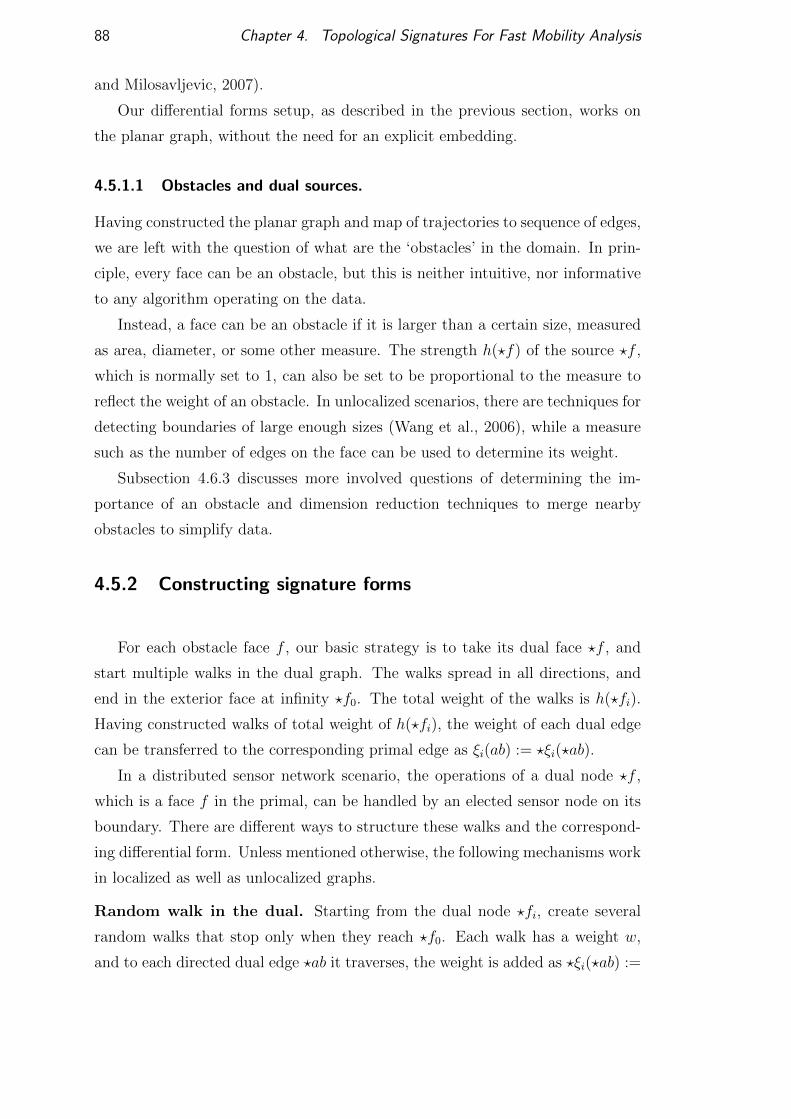
88 Chapter 4. Topological Signatures For Fast Mobility Analysis
and Milosavljevic, 2007).
Our differential forms setup, as described in the previous section, works on
the planar graph, without the need for an explicit embedding.
4.5.1.1 Obstacles and dual sources.
Having constructed the planar graph and map of trajectories to sequence of edges,
we are left with the question of what are the ‘obstacles’ in the domain. In prin-
ciple, every face can be an obstacle, but this is neither intuitive, nor informative
to any algorithm operating on the data.
Instead, a face can be an obstacle if it is larger than a certain size, measured
as area, diameter, or some other measure. The strength h(?f) of the source ?f ,
which is normally set to 1, can also be set to be proportional to the measure to
reflect the weight of an obstacle. In unlocalized scenarios, there are techniques for
detecting boundaries of large enough sizes (Wang et al., 2006), while a measure
such as the number of edges on the face can be used to determine its weight.
Subsection 4.6.3 discusses more involved questions of determining the im-
portance of an obstacle and dimension reduction techniques to merge nearby
obstacles to simplify data.
4.5.2 Constructing signature forms
For each obstacle face f , our basic strategy is to take its dual face ?f , and
start multiple walks in the dual graph. The walks spread in all directions, and
end in the exterior face at infinity ?f0. The total weight of the walks is h(?fi).
Having constructed walks of total weight of h(?fi), the weight of each dual edge
can be transferred to the corresponding primal edge as ξi(ab) := ?ξi(?ab).
In a distributed sensor network scenario, the operations of a dual node ?f ,
which is a face f in the primal, can be handled by an elected sensor node on its
boundary. There are different ways to structure these walks and the correspond-
ing differential form. Unless mentioned otherwise, the following mechanisms work
in localized as well as unlocalized graphs.
Random walk in the dual. Starting from the dual node ?fi, create several
random walks that stop only when they reach ?f0. Each walk has a weight w,
and to each directed dual edge ?ab it traverses, the weight is added as ?ξi(?ab) :=
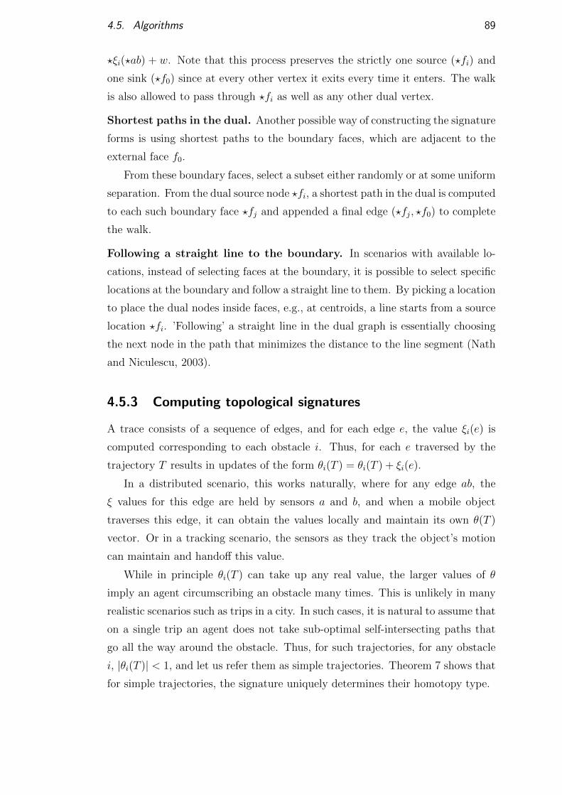
4.5. Algorithms 89
?ξi(?ab) + w. Note that this process preserves the strictly one source (?fi) and
one sink (?f0) since at every other vertex it exits every time it enters. The walk
is also allowed to pass through ?fi as well as any other dual vertex.
Shortest paths in the dual. Another possible way of constructing the signature
forms is using shortest paths to the boundary faces, which are adjacent to the
external face f0.
From these boundary faces, select a subset either randomly or at some uniform
separation. From the dual source node ?fi, a shortest path in the dual is computed
to each such boundary face ?fj and appended a final edge (?fj, ?f0) to complete
the walk.
Following a straight line to the boundary. In scenarios with available lo-
cations, instead of selecting faces at the boundary, it is possible to select specific
locations at the boundary and follow a straight line to them. By picking a location
to place the dual nodes inside faces, e.g., at centroids, a line starts from a source
location ?fi. ’Following’ a straight line in the dual graph is essentially choosing
the next node in the path that minimizes the distance to the line segment (Nath
and Niculescu, 2003).
4.5.3 Computing topological signatures
A trace consists of a sequence of edges, and for each edge e, the value ξi(e) is
computed corresponding to each obstacle i. Thus, for each e traversed by the
trajectory T results in updates of the form θi(T ) = θi(T ) + ξi(e).
In a distributed scenario, this works naturally, where for any edge ab, the
ξ values for this edge are held by sensors a and b, and when a mobile object
traverses this edge, it can obtain the values locally and maintain its own θ(T )
vector. Or in a tracking scenario, the sensors as they track the object’s motion
can maintain and handoff this value.
While in principle θi(T ) can take up any real value, the larger values of θ
imply an agent circumscribing an obstacle many times. This is unlikely in many
realistic scenarios such as trips in a city. In such cases, it is natural to assume that
on a single trip an agent does not take sub-optimal self-intersecting paths that
go all the way around the obstacle. Thus, for such trajectories, for any obstacle
i, |θi(T )| < 1, and let us refer them as simple trajectories. Theorem 7 shows that
for simple trajectories, the signature uniquely determines their homotopy type.
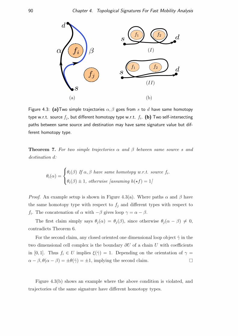
90 Chapter 4. Topological Signatures For Fast Mobility Analysis
(a) (b)
Figure 4.3: (a)Two simple trajectories α, β goes from s to d have same homotopy
type w.r.t. source fj, but different homotopy type w.r.t. fi. (b) Two self-intersecting
paths between same source and destination may have same signature value but dif-
ferent homotopy type.
Theorem 7. For two simple trajectories α and β between same source s and
destination d:
θi(α) =
θi(β) If α, β have same homotopy w.r.t. source fi.
θi(β)± 1, otherwise [assuming h(?f) = 1]
Proof. An example setup is shown in Figure 4.3(a). Where paths α and β have
the same homotopy type with respect to fj and different types with respect to
fi. The concatenation of α with −β gives loop γ = α− β.
The first claim simply says θj(α) = θj(β), since otherwise θj(α − β) 6= 0,
contradicts Theorem 6.
For the second claim, any closed oriented one dimensional loop object γ in the
two dimensional cell complex is the boundary ∂U of a chain U with coefficients
in [0, 1]. Thus fi ∈ U implies ξ(γ) = 1. Depending on the orientation of γ =
α− β, θ(α− β) = ±θ(γ) = ±1, implying the second claim.
Figure 4.3(b) shows an example where the above condition is violated, and
trajectories of the same signature have different homotopy types.
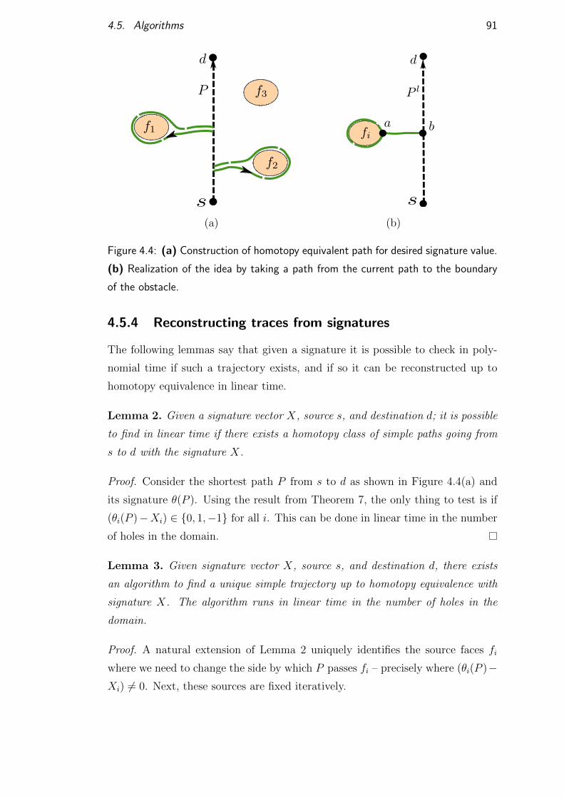
4.5. Algorithms 91
(a) (b)
Figure 4.4: (a) Construction of homotopy equivalent path for desired signature value.
(b) Realization of the idea by taking a path from the current path to the boundary
of the obstacle.
4.5.4 Reconstructing traces from signatures
The following lemmas say that given a signature it is possible to check in poly-
nomial time if such a trajectory exists, and if so it can be reconstructed up to
homotopy equivalence in linear time.
Lemma 2. Given a signature vector X, source s, and destination d; it is possible
to find in linear time if there exists a homotopy class of simple paths going from
s to d with the signature X.
Proof. Consider the shortest path P from s to d as shown in Figure 4.4(a) and
its signature θ(P ). Using the result from Theorem 7, the only thing to test is if
(θi(P )−Xi) ∈ {0, 1,−1} for all i. This can be done in linear time in the number
of holes in the domain.
Lemma 3. Given signature vector X, source s, and destination d, there exists
an algorithm to find a unique simple trajectory up to homotopy equivalence with
signature X. The algorithm runs in linear time in the number of holes in the
domain.
Proof. A natural extension of Lemma 2 uniquely identifies the source faces fi
where we need to change the side by which P passes fi – precisely where (θi(P )−Xi) 6= 0. Next, these sources are fixed iteratively.
92 Chapter 4. Topological Signatures For Fast Mobility Analysis
Initialize this process by setting the path P as the shortest path from s to
d. Suppose at iteration l, the path is P l and the next obstacle to fix is fi.
Consider an arbitrary node b ∈ P l, and another arbitrary node a ∈ ∂fi as shown
in Figure 4.4(b). Now P l+1 is the concatenation of the following path segments:
s to b, b to a, a to a (along ∂fi), a to b, and finally b to d. So, the path P l+1 has
now right homotopy type w.r.t. fi.
This construction essentially determines the homotopy type from the signa-
ture. Given that, we can now compute a short path in that class using well known
algorithms in computational geometry (Hershberger and Snoeyink, 1994a).
4.6 Applications and Optimizations
Here we discuss how the topological signatures can be designed and implemented
for better applied analytics.
4.6.1 Nearest neighbor search and Locality Sensitive Hashing
A fundamental question in data analysis is the search for nearest neighbor, or k
nearest neighbors, which forms the basis of several classification and clustering
techniques and queries on noisy data. In case of trajectories, searching for near-
est neighbors is expensive due to the fundamental cost of comparing two long
trajectories (Alt and Godau, 1995).
Locality sensitive hashing (LSH) is used in data mining to accelerate the search
for nearest neighbors. However, defining LSH for trajectories is a non trivial
problem, as is constructing computationally efficient hash functions (Driemel and
Silvestri, 2017). We want to instead use representations of trajectories as points
in the Euclidean space, where good LSH techniques are known.
A standard LSH scheme (Datar et al., 2004) uses a hash function h constructed
as follows. Select a random straight line in Rk. Then project each data point
linearly onto the line. Partition the line into segments of length w for some given
w, and treat each segment as a “bucket”. Nearby data points are likely to hash
into the same bucket, while far apart points are likely to hash to different ones.
Given a query point q, we can perform the same projection and hashing, and then
search for its nearest neighbor in the bucket containing q. Expensive methods (Alt
and Godau, 1995) can be used for this search since the pruned candidate set
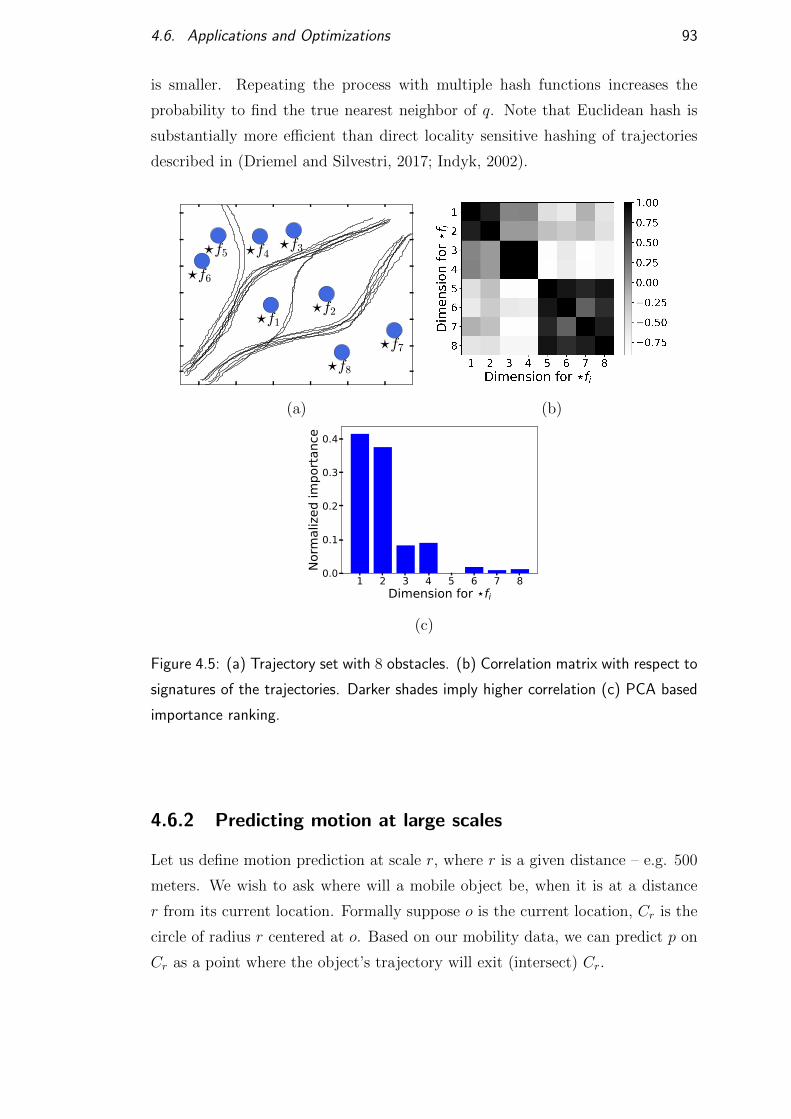
4.6. Applications and Optimizations 93
is smaller. Repeating the process with multiple hash functions increases the
probability to find the true nearest neighbor of q. Note that Euclidean hash is
substantially more efficient than direct locality sensitive hashing of trajectories
described in (Driemel and Silvestri, 2017; Indyk, 2002).
f1
f2
f3f4f5
f6
f7
f8
(a) (b)
1 2 3 4 5 6 7 8Dimension for fi
0.0
0.1
0.2
0.3
0.4
Norm
alize
d im
porta
nce
(c)
Figure 4.5: (a) Trajectory set with 8 obstacles. (b) Correlation matrix with respect to
signatures of the trajectories. Darker shades imply higher correlation (c) PCA based
importance ranking.
4.6.2 Predicting motion at large scales
Let us define motion prediction at scale r, where r is a given distance – e.g. 500
meters. We wish to ask where will a mobile object be, when it is at a distance
r from its current location. Formally suppose o is the current location, Cr is the
circle of radius r centered at o. Based on our mobility data, we can predict p on
Cr as a point where the object’s trajectory will exit (intersect) Cr.
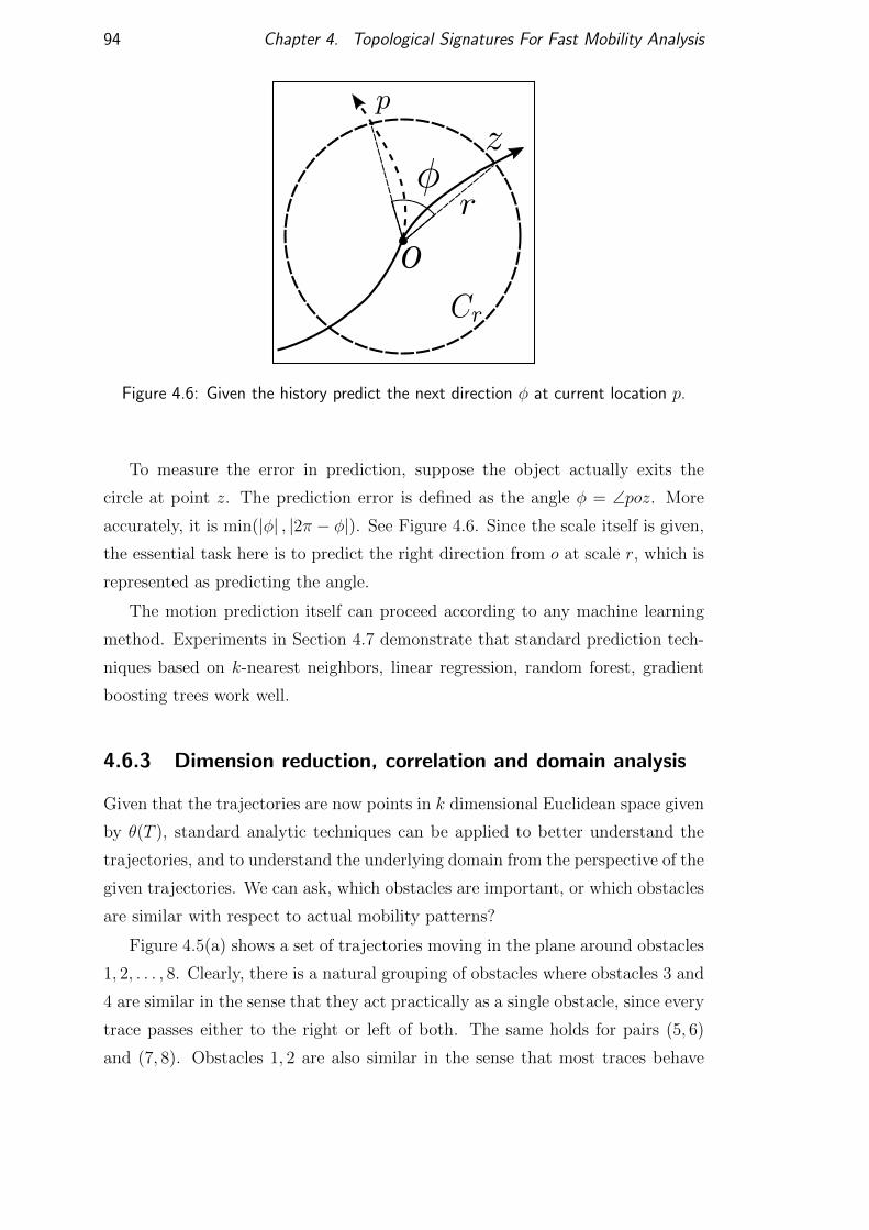
94 Chapter 4. Topological Signatures For Fast Mobility Analysis
Figure 4.6: Given the history predict the next direction φ at current location p.
To measure the error in prediction, suppose the object actually exits the
circle at point z. The prediction error is defined as the angle φ = ∠poz. More
accurately, it is min(|φ| , |2π − φ|). See Figure 4.6. Since the scale itself is given,
the essential task here is to predict the right direction from o at scale r, which is
represented as predicting the angle.
The motion prediction itself can proceed according to any machine learning
method. Experiments in Section 4.7 demonstrate that standard prediction tech-
niques based on k-nearest neighbors, linear regression, random forest, gradient
boosting trees work well.
4.6.3 Dimension reduction, correlation and domain analysis
Given that the trajectories are now points in k dimensional Euclidean space given
by θ(T ), standard analytic techniques can be applied to better understand the
trajectories, and to understand the underlying domain from the perspective of the
given trajectories. We can ask, which obstacles are important, or which obstacles
are similar with respect to actual mobility patterns?
Figure 4.5(a) shows a set of trajectories moving in the plane around obstacles
1, 2, . . . , 8. Clearly, there is a natural grouping of obstacles where obstacles 3 and
4 are similar in the sense that they act practically as a single obstacle, since every
trace passes either to the right or left of both. The same holds for pairs (5, 6)
and (7, 8). Obstacles 1, 2 are also similar in the sense that most traces behave

4.6. Applications and Optimizations 95
similarly with respect to both, with only a few passing between them.
These intuitive results can be obtained from standard analytic and visual-
ization methods. Figure 4.5(b) shows the correlation matrix of θ, where darker
shades indicate higher correlation. The correlation lets us have a more abstract
view of the domain, where related nearby holes can be viewed as one.
Techniques like Principal Component Analysis can be applied to the Euclidean
data to determine which dimensions record larger variance – implying larger vari-
ability in how traces traverse the obstacles. We apply this idea to get the intuitive
result in Figure 4.5(c) that obstacles 1 and 2 are clearly more significant than
others as they split a large body of motions.
Greedy filtration of obstacles. A different strategy which is found effective
in experiments, is to greedily select obstacles (dual sources) that maximize the
accuracy for the task at hand.
For example, for nearest neighbor search, this accuracy can be defined as the
fraction of times that the true Frechet nearest neighbor is contained among the
m nearest neighbors. The greedy strategy will iteratively select the obstacle that
maximizes the total accuracy over all pairs, until it has selected some k obstacles.
For scenarios with large number of obstacle, similar strategies can be implemented
for distributed cluster computation (Mirzasoleiman et al., 2016). The benefit of
this heavy computation is that the signatures become more compact and assuming
the dataset is representative of typical motion, future computations of signatures,
nearest neighbors, predictions etc will be more efficient.
4.6.4 Adaptive resolution signatures
It is natural to ask for representations that give greater weight to recent infor-
mation and less weight to history, for example, for short term prediction. The
signatures can be seamlessly adapted to achieve this using weighted averaging.
Where for each edge traversed by the trajectory, we modify the update rule to
be θi(T ) = β.θi(T ) + (1 − β)ξi(e) for a constant β : 0 < β < 1 that determines
the weight of history in the signature.
In the example in Figure 4.7(a) at point o, the adaptively weighted signature
finds the set γ to be currently more relevant to the query α.
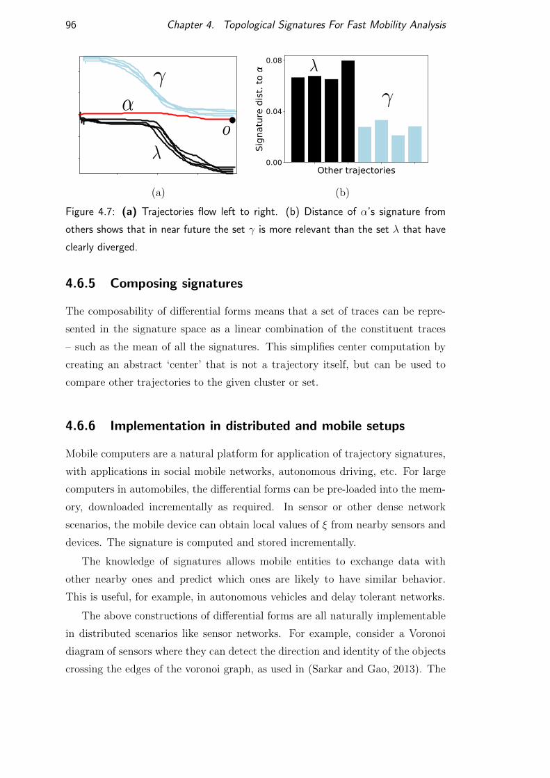
96 Chapter 4. Topological Signatures For Fast Mobility Analysis
Other trajectories0.00
0.04
0.08
Sig
natu
re d
ist.
to
(a) (b)
Figure 4.7: (a) Trajectories flow left to right. (b) Distance of α’s signature from
others shows that in near future the set γ is more relevant than the set λ that have
clearly diverged.
4.6.5 Composing signatures
The composability of differential forms means that a set of traces can be repre-
sented in the signature space as a linear combination of the constituent traces
– such as the mean of all the signatures. This simplifies center computation by
creating an abstract ‘center’ that is not a trajectory itself, but can be used to
compare other trajectories to the given cluster or set.
4.6.6 Implementation in distributed and mobile setups
Mobile computers are a natural platform for application of trajectory signatures,
with applications in social mobile networks, autonomous driving, etc. For large
computers in automobiles, the differential forms can be pre-loaded into the mem-
ory, downloaded incrementally as required. In sensor or other dense network
scenarios, the mobile device can obtain local values of ξ from nearby sensors and
devices. The signature is computed and stored incrementally.
The knowledge of signatures allows mobile entities to exchange data with
other nearby ones and predict which ones are likely to have similar behavior.
This is useful, for example, in autonomous vehicles and delay tolerant networks.
The above constructions of differential forms are all naturally implementable
in distributed scenarios like sensor networks. For example, consider a Voronoi
diagram of sensors where they can detect the direction and identity of the objects
crossing the edges of the voronoi graph, as used in (Sarkar and Gao, 2013). The
4.7. Experiments 97
sensors maintain the weights on the edges giving the differential forms and as
an object moves between cells, its signature is handed off (similar to hand-off in
cellular network) to the successive sensor. An alternative approach could be for
the sensors to record and store the edge crossings of mobile objects, and compute
the signature on demand by summing along the handoff path.
4.7 Experiments
In this section, we show experimental evidence that the topological signatures
simplify the representation of trajectories and also perform well in clustering,
prediction, and other tasks. The main observations are:
• Nearest neighbor of a query trajectory according to Frechet distance can
be found efficiently using fast Locality Sensitive Hashing and pruning on
topological signatures.
• Motion prediction of trajectories is accurate and efficient. It achieves similar
accuracy as Long Short Term Memory neural networks (henceforth LSTM),
but provides much faster training and query time. Prediction results are
verified using two real mobility datasets.
• Greedy source selection reduces dimension to get compact signatures, with
minimal loss in quality of analytic results.
• Popular paths or paths with the most number of trajectories in a given
region can be estimated by kernel density estimation on signatures.
• Topological signature based method is robust to sparse, noisy trajectories;
it can predict future direction of mobile objects accurately in trajectories
with many missing data points.
4.7.1 Experimental setup
Datasets. We use two publicly available datasets: Rome Taxi dataset (Bracciale
et al., 2014) and Porto Dataset1. While the former has trajectories of 320 taxis
1https://www.kaggle.com/c/pkdd-15-predict-taxi-service-trajectory-i
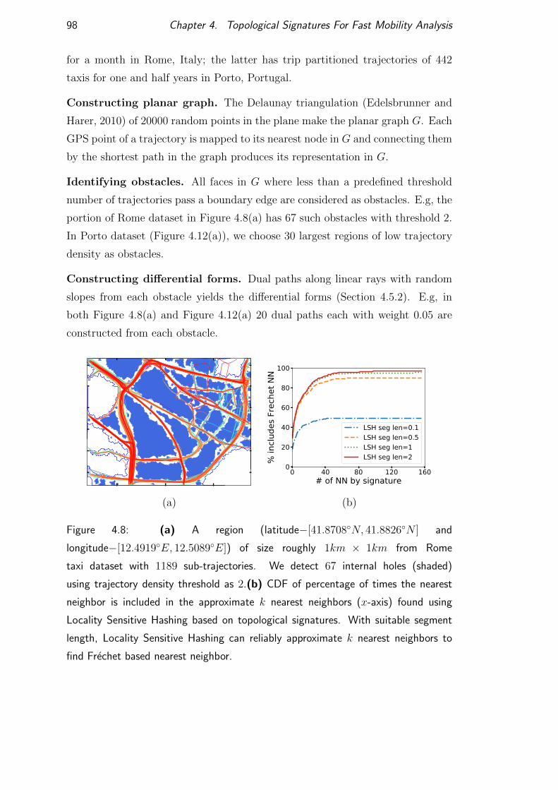
98 Chapter 4. Topological Signatures For Fast Mobility Analysis
for a month in Rome, Italy; the latter has trip partitioned trajectories of 442
taxis for one and half years in Porto, Portugal.
Constructing planar graph. The Delaunay triangulation (Edelsbrunner and
Harer, 2010) of 20000 random points in the plane make the planar graph G. Each
GPS point of a trajectory is mapped to its nearest node in G and connecting them
by the shortest path in the graph produces its representation in G.
Identifying obstacles. All faces in G where less than a predefined threshold
number of trajectories pass a boundary edge are considered as obstacles. E.g, the
portion of Rome dataset in Figure 4.8(a) has 67 such obstacles with threshold 2.
In Porto dataset (Figure 4.12(a)), we choose 30 largest regions of low trajectory
density as obstacles.
Constructing differential forms. Dual paths along linear rays with random
slopes from each obstacle yields the differential forms (Section 4.5.2). E.g, in
both Figure 4.8(a) and Figure 4.12(a) 20 dual paths each with weight 0.05 are
constructed from each obstacle.
0 40 80 120 160# of NN by signature
0
20
40
60
80
100
% in
clude
s Fre
chet
NN
LSH seg len=0.1LSH seg len=0.5LSH seg len=1LSH seg len=2
(a) (b)
Figure 4.8: (a) A region (latitude−[41.8708◦N, 41.8826◦N ] and
longitude−[12.4919◦E, 12.5089◦E]) of size roughly 1km × 1km from Rome
taxi dataset with 1189 sub-trajectories. We detect 67 internal holes (shaded)
using trajectory density threshold as 2.(b) CDF of percentage of times the nearest
neighbor is included in the approximate k nearest neighbors (x-axis) found using
Locality Sensitive Hashing based on topological signatures. With suitable segment
length, Locality Sensitive Hashing can reliably approximate k nearest neighbors to
find Frechet based nearest neighbor.
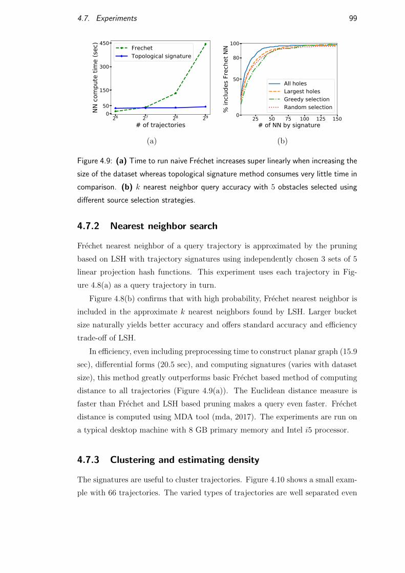
4.7. Experiments 99
26 27 28 29
# of trajectories0
50
150
300
450
NN c
ompu
te ti
me
(sec
)
FrechetTopological signature
25 50 75 100 125 150# of NN by signature
0
50
80
100
% in
clude
s Fre
chet
NN
All holesLargest holesGreedy selectionRandom selection
(a) (b)
Figure 4.9: (a) Time to run naive Frechet increases super linearly when increasing the
size of the dataset whereas topological signature method consumes very little time in
comparison. (b) k nearest neighbor query accuracy with 5 obstacles selected using
different source selection strategies.
4.7.2 Nearest neighbor search
Frechet nearest neighbor of a query trajectory is approximated by the pruning
based on LSH with trajectory signatures using independently chosen 3 sets of 5
linear projection hash functions. This experiment uses each trajectory in Fig-
ure 4.8(a) as a query trajectory in turn.
Figure 4.8(b) confirms that with high probability, Frechet nearest neighbor is
included in the approximate k nearest neighbors found by LSH. Larger bucket
size naturally yields better accuracy and offers standard accuracy and efficiency
trade-off of LSH.
In efficiency, even including preprocessing time to construct planar graph (15.9
sec), differential forms (20.5 sec), and computing signatures (varies with dataset
size), this method greatly outperforms basic Frechet based method of computing
distance to all trajectories (Figure 4.9(a)). The Euclidean distance measure is
faster than Frechet and LSH based pruning makes a query even faster. Frechet
distance is computed using MDA tool (mda, 2017). The experiments are run on
a typical desktop machine with 8 GB primary memory and Intel i5 processor.
4.7.3 Clustering and estimating density
The signatures are useful to cluster trajectories. Figure 4.10 shows a small exam-
ple with 66 trajectories. The varied types of trajectories are well separated even
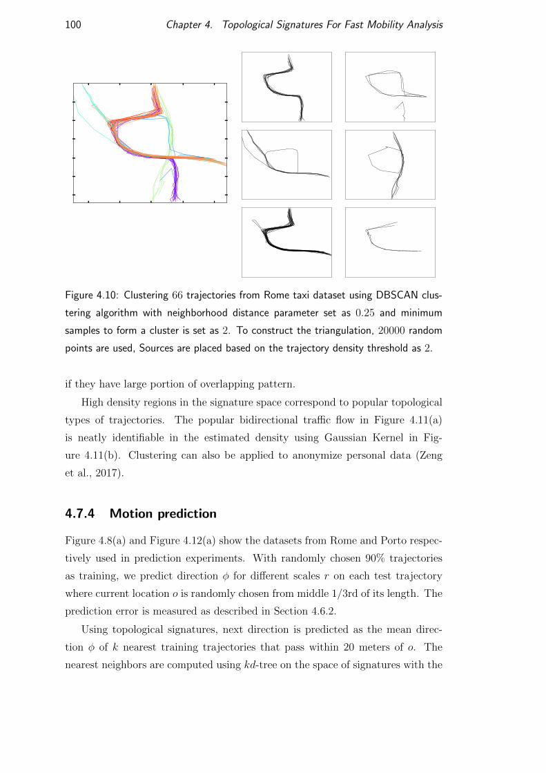
100 Chapter 4. Topological Signatures For Fast Mobility Analysis
Figure 4.10: Clustering 66 trajectories from Rome taxi dataset using DBSCAN clus-
tering algorithm with neighborhood distance parameter set as 0.25 and minimum
samples to form a cluster is set as 2. To construct the triangulation, 20000 random
points are used, Sources are placed based on the trajectory density threshold as 2.
if they have large portion of overlapping pattern.
High density regions in the signature space correspond to popular topological
types of trajectories. The popular bidirectional traffic flow in Figure 4.11(a)
is neatly identifiable in the estimated density using Gaussian Kernel in Fig-
ure 4.11(b). Clustering can also be applied to anonymize personal data (Zeng
et al., 2017).
4.7.4 Motion prediction
Figure 4.8(a) and Figure 4.12(a) show the datasets from Rome and Porto respec-
tively used in prediction experiments. With randomly chosen 90% trajectories
as training, we predict direction φ for different scales r on each test trajectory
where current location o is randomly chosen from middle 1/3rd of its length. The
prediction error is measured as described in Section 4.6.2.
Using topological signatures, next direction is predicted as the mean direc-
tion φ of k nearest training trajectories that pass within 20 meters of o. The
nearest neighbors are computed using kd-tree on the space of signatures with the
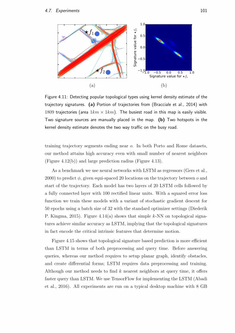
4.7. Experiments 101
f1
f2 1.0 0.5 0.0 0.5 1.0Signature value for f1
1.0
0.5
0.0
0.5
1.0
Sig
natu
re v
alu
e f
or
f 2
(a) (b)
Figure 4.11: Detecting popular topological types using kernel density estimate of the
trajectory signatures. (a) Portion of trajectories from (Bracciale et al., 2014) with
1809 trajectories (area 1km × 1km). The busiest road in this map is easily visible.
Two signature sources are manually placed in the map. (b) Two hotspots in the
kernel density estimate denotes the two way traffic on the busy road.
training trajectory segments ending near o. In both Porto and Rome datasets,
our method attains high accuracy even with small number of nearest neighbors
(Figure 4.12(b)) and large prediction radius (Figure 4.13).
As a benchmark we use neural networks with LSTM as regressors (Gers et al.,
2000) to predict φ, given equi-spaced 20 locations on the trajectory between o and
start of the trajectory. Each model has two layers of 20 LSTM cells followed by
a fully connected layer with 100 rectified linear units. With a squared error loss
function we train these models with a variant of stochastic gradient descent for
50 epochs using a batch size of 32 with the standard optimizer settings (Diederik
P. Kingma, 2015). Figure 4.14(a) shows that simple k-NN on topological signa-
tures achieve similar accuracy as LSTM, implying that the topological signatures
in fact encode the critical intrinsic features that determine motion.
Figure 4.15 shows that topological signature based prediction is more efficient
than LSTM in terms of both preprocessing and query time. Before answering
queries, whereas our method requires to setup planar graph, identify obstacles,
and create differential forms; LSTM requires data preprocessing and training.
Although our method needs to find k nearest neighbors at query time, it offers
faster query than LSTM. We use TensorFlow for implementing the LSTM (Abadi
et al., 2016). All experiments are run on a typical desktop machine with 8 GB
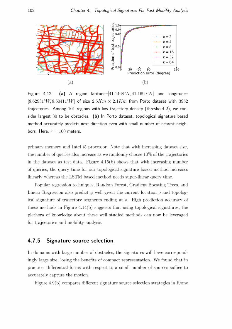
102 Chapter 4. Topological Signatures For Fast Mobility Analysis
0 30 60 90 180Prediction error (degree)
0.0
0.5
0.80.91.0
Frac
tion
of te
st tr
ajec
torie
s
k = 2k = 4k = 8k = 16k = 32k = 64
(a) (b)
Figure 4.12: (a) A region latitude–[41.1468◦N, 41.1699◦N ] and longitude–
[8.62931◦W, 8.60411◦W ] of size 2.5Km × 2.1Km from Porto dataset with 3952
trajectories. Among 101 regions with low trajectory density (threshold 2), we con-
sider largest 30 to be obstacles. (b) In Porto dataset, topological signature based
method accurately predicts next direction even with small number of nearest neigh-
bors. Here, r = 100 meters.
primary memory and Intel i5 processor. Note that with increasing dataset size,
the number of queries also increase as we randomly choose 10% of the trajectories
in the dataset as test data. Figure 4.15(b) shows that with increasing number
of queries, the query time for our topological signature based method increases
linearly whereas the LSTM based method needs super-linear query time.
Popular regression techniques, Random Forest, Gradient Boosting Trees, and
Linear Regression also predict φ well given the current location o and topolog-
ical signature of trajectory segments ending at o. High prediction accuracy of
these methods in Figure 4.14(b) suggests that using topological signatures, the
plethora of knowledge about these well studied methods can now be leveraged
for trajectories and mobility analysis.
4.7.5 Signature source selection
In domains with large number of obstacles, the signatures will have correspond-
ingly large size, losing the benefits of compact representation. We found that in
practice, differential forms with respect to a small number of sources suffice to
accurately capture the motion.
Figure 4.9(b) compares different signature source selection strategies in Rome
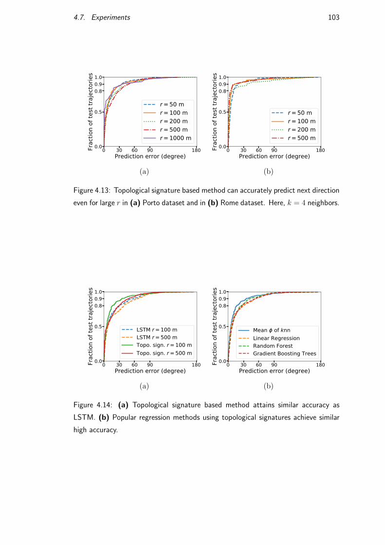
4.7. Experiments 103
0 30 60 90 180Prediction error (degree)
0.0
0.5
0.80.91.0
Frac
tion
of te
st tr
ajec
torie
s
r = 50 mr = 100 mr = 200 mr = 500 mr = 1000 m
0 30 60 90 180Prediction error (degree)
0.0
0.5
0.80.91.0
Frac
tion
of te
st tr
ajec
torie
s
r = 50 mr = 100 mr = 200 mr = 500 m
(a) (b)
Figure 4.13: Topological signature based method can accurately predict next direction
even for large r in (a) Porto dataset and in (b) Rome dataset. Here, k = 4 neighbors.
0 30 60 90 180Prediction error (degree)
0.0
0.5
0.80.91.0
Frac
tion
of te
st tr
ajec
torie
s
LSTM r = 100 mLSTM r = 500 mTopo. sign. r = 100 mTopo. sign. r = 500 m
0 30 60 90 180Prediction error (degree)
0.0
0.5
0.80.91.0
Frac
tion
of te
st tr
ajec
torie
s
Mean of knnLinear RegressionRandom ForestGradient Boosting Trees
(a) (b)
Figure 4.14: (a) Topological signature based method attains similar accuracy as
LSTM. (b) Popular regression methods using topological signatures achieve similar
high accuracy.
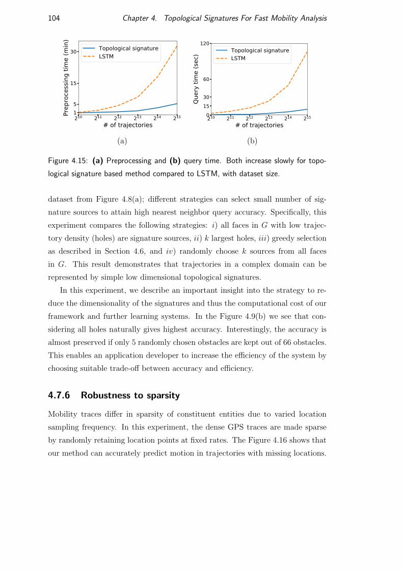
104 Chapter 4. Topological Signatures For Fast Mobility Analysis
210 211 212 213 214 215
# of trajectories15
15
30
Prep
roce
ssin
g tim
e (m
in)
Topological signatureLSTM
210 211 212 213 214 215
# of trajectories0
1530
60
120
Quer
y tim
e (s
ec) Topological signature
LSTM
(a) (b)
Figure 4.15: (a) Preprocessing and (b) query time. Both increase slowly for topo-
logical signature based method compared to LSTM, with dataset size.
dataset from Figure 4.8(a); different strategies can select small number of sig-
nature sources to attain high nearest neighbor query accuracy. Specifically, this
experiment compares the following strategies: i) all faces in G with low trajec-
tory density (holes) are signature sources, ii) k largest holes, iii) greedy selection
as described in Section 4.6, and iv) randomly choose k sources from all faces
in G. This result demonstrates that trajectories in a complex domain can be
represented by simple low dimensional topological signatures.
In this experiment, we describe an important insight into the strategy to re-
duce the dimensionality of the signatures and thus the computational cost of our
framework and further learning systems. In the Figure 4.9(b) we see that con-
sidering all holes naturally gives highest accuracy. Interestingly, the accuracy is
almost preserved if only 5 randomly chosen obstacles are kept out of 66 obstacles.
This enables an application developer to increase the efficiency of the system by
choosing suitable trade-off between accuracy and efficiency.
4.7.6 Robustness to sparsity
Mobility traces differ in sparsity of constituent entities due to varied location
sampling frequency. In this experiment, the dense GPS traces are made sparse
by randomly retaining location points at fixed rates. The Figure 4.16 shows that
our method can accurately predict motion in trajectories with missing locations.

4.7. Experiments 105
0 30 60 90 180Prediction error (degree)
0.0
0.5
0.80.91.0
Frac
tion
of te
st tr
ajec
torie
s
probretain = 0.3probretain = 0.5probretain = 0.7probretain = 1.0
Figure 4.16: Predicting locations with sparse trajectories: Each location point is re-
tained with certain probability in each trajectory. Our method achieves high prediction
accuracy even with sparse trajectory.

Chapter 5
Publishing Differentially Private
Spatial Data From Distributed
Sensors
This chapter focuses on publishing sanitized location stamps of independent
events recorded by spatially distributed sensors. We design differential privacy
mechanisms for two scenarios, to protect accurate locations of the events and
their occurrences. Proposed mechanisms are based on location displacement and
inclusion of fake events. They are designed to maintain a balance between privacy
and utility for spatial range queries. Our algorithms allow distributed operation
and maintains utility for any number of queries.
Previously in Chapter 3 we discussed how to protect event timings in a time
series. Here, we do not consider the temporal attributes in the events and describe
how to protect privacy for their spatial attributes. All these mechanisms can be
augmented with the algorithms in Chapter 3 to attain privacy for spatiotemporal
range queries.
5.1 Introduction
Here, we are concerned about the data collected by distributed sensors. Examples
of such data include location snapshots of a population, events detected by traffic
sensors, occupancy and motion sensing information etc. After the collection,
events are delivered to the aggregator services, where they are subject to queries
and analysis by users of the service. In the process, implicit sensitive information
107
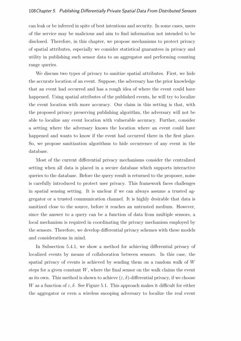
108Chapter 5. Publishing Differentially Private Spatial Data From Distributed Sensors
can leak or be inferred in spite of best intentions and security. In some cases, users
of the service may be malicious and aim to find information not intended to be
disclosed. Therefore, in this chapter, we propose mechanisms to protect privacy
of spatial attributes, especially we consider statistical guarantees in privacy and
utility in publishing such sensor data to an aggregator and performing counting
range queries.
We discuss two types of privacy to sanitize spatial attributes. First, we hide
the accurate location of an event. Suppose, the adversary has the prior knowledge
that an event had occurred and has a rough idea of where the event could have
happened. Using spatial attributes of the published events, he will try to localize
the event location with more accuracy. Our claim in this setting is that, with
the proposed privacy preserving publishing algorithm, the adversary will not be
able to localize any event location with vulnerable accuracy. Further, consider
a setting where the adversary knows the location where an event could have
happened and wants to know if the event had occurred there in the first place.
So, we propose sanitization algorithms to hide occurrence of any event in the
database.
Most of the current differential privacy mechanisms consider the centralized
setting when all data is placed in a secure database which supports interactive
queries to the database. Before the query result is returned to the proposer, noise
is carefully introduced to protect user privacy. This framework faces challenges
in spatial sensing setting. It is unclear if we can always assume a trusted ag-
gregator or a trusted communication channel. It is highly desirable that data is
sanitized close to the source, before it reaches an untrusted medium. However,
since the answer to a query can be a function of data from multiple sensors, a
local mechanism is required in coordinating the privacy mechanism employed by
the sensors. Therefore, we develop differential privacy schemes with these models
and considerations in mind.
In Subsection 5.4.1, we show a method for achieving differential privacy of
localized events by means of collaboration between sensors. In this case, the
spatial privacy of events is achieved by sending them on a random walk of W
steps for a given constant W , where the final sensor on the walk claims the event
as its own. This method is shown to achieve (ε, δ)-differential privacy, if we choose
W as a function of ε, δ. See Figure 5.1. This approach makes it difficult for either
the aggregator or even a wireless snooping adversary to localize the real event
5.1. Introduction 109
s
s′
Figure 5.1: To avoid the aggregator/collector knowing the location of the sensor
generating the event, the source s uses a random walk to send the message to a node
s′ who delivers to the aggregator instead. The nodes in the network might also report
fake events as shown in gray arrows.
source. From system perspective, this mechanism protects against untrusted
aggregator but needs the inter-sensor communication channel to be trusted.
When the inter-sensor communication is also vulnerable then it is difficult
to apply the above random walk mechanism. Here, we develop a mechanism
involving a stream of spurious, or fake events introduced from a Poisson process
with a rate λ dependent on the privacy requirement. This mechanism is an
extension of the fake event augmentation mechanism discussed in Chapter 3 in
2D spatial dimension. This approach is proved to provide differential privacy
of counting range queries for λ = O(
1ε2
log 1δ
), while providing accurate results.
One nice property is that the intensity magnitude λ of the added noise is only
relevant to the privacy guarantee and the absolute error in data utility, and is
independent of the real event distribution.
In Section 5.5, we experimentally compare the utility of our algorithms against
the local privacy mechanism proposed in (Chan et al., 2011). Although the
method was developed for 1D temporal sequences, we extend it to 2D spatial
range queries for our purposes in Subsection 5.4.3. However, this mechanism is
not suitable for publishing data. We use a real world dataset of geo-located tweets
in and around London. Experiments show that our approaches provide accurate
results for range queries in all cases.
In the following, we first discuss the existing research results in Section 5.2,
background material and models in Section 5.3 before moving on to the algo-
rithms.
110Chapter 5. Publishing Differentially Private Spatial Data From Distributed Sensors
5.2 Related Work
Differential privacy was first proposed in (Dwork et al., 2006), where user data
are collected by a trusted aggregator and Laplace noise are added before the
aggregator releases the data to achieve differential privacy. After that, there has
been a plethora of works on releasing different types of data under differential
privacy.
(Andres et al., 2013) introduced geo-indistinguishibility, a generalized version
of differential privacy for location information, where using planar Laplace noise,
any two locations within a given distance produce observations with similar dis-
tributions. Differentially private data aggregation in crowd sensing system is
analyzed in (Jin et al., 2016; Yang et al., 2018).
Spatial decomposition under differential privacy. (Cormode et al., 2012)
proposed a geometric budget strategy, adding noise with geometric distribution
at each level of quad-tree for private spatial range queries. If h is the height of
the tree (leaves are on level 0), then Lap(εi) noise is added to the true count
of each quad-cell on level i, where εi = 2(h−i)/3 3√2−12(h+1)/3−1
. The upper bound for
the variance of a range query is 2h+7/ε2. (Qardaji et al., 2013) analyzed query
errors on uniform grids, which consists of two sources of errors. One is the error
is introduced by adding random noise from Laplace distribution, and the other
from the assumption that the data points are distributed uniformly in a cell.
If there are N points and the domain is partitioned into a m × m uniform
grid, the error, determined by standard deviation, is√
2rm/ε+√rN/mc0, where
r is the ratio of the area of the query over the whole domain, c0 is constant.
To minimize the error, m = O(√Nε) is suggested. They further proposed an
adaptive grids methods to adjust the size of the grids considering the density of
data. Further works on uniform grids can also be found in (Wang et al., 2018).
Local differential privacy. Most works under differential privacy are in the
setting of central model, where a trusted aggregator is present. In the notion of
local differential privacy, first proposed by (Kasiviswanathan et al., 2011), data
sources sanitize their own data with differential privacy mechanism before sharing
with the aggregator. It is widely adopted, for example in (Erlingsson et al., 2014;
Bittau et al., 2017). However, the partial sum mechanism does not suit our
purpose of data publishing as the amount of noise is decided based on the query.

5.3. Models and problem descriptions 111
5.3 Models and problem descriptions
5.3.1 System Model
The typical entities in a distributed sensing scenario are:
• Sensors : A sensor detects events generated in the physical environment.
This detection could be through wireless connectivity, from visual sensing,
or other sensing modalities. We assume that the sensors detecting the events
are connected by suitable communication technology.
• Aggregators : an aggregator is a service provider who collects data from the
sensors and responds to an aggregation query, such as a range counting
query – report the number of events that happened within a geographical
domain.
• Query makers : A user can issue queries to the aggregator to infer knowledge
about the event counts and patterns.
In a typical setup, data from sensors are sent to the aggregator. The query
maker then queries the aggregator to obtain information. The data that the
sensors transmit can be raw data, or aggregated ones. Depending on the trust-
worthiness of the aggregator or communication channels, the sensors may need
to sanitize data before transmission.
5.3.2 Trust Model
Depending on the applications, there could be different levels of trust between
the entities:
• Trusted aggregator. The most trusted scenario, where the aggregators and
all communications upto them are trusted and secure. This is closest to
the common differential privacy model, where only the query maker is un-
trusted, and the aggregator can perform centralized computations on col-
lected data. We do not design algorithms for this setting in this chapter,
but we compare with solutions of this setting in the evaluation section.
• Trusted sensors. In this model, the sensors trust each other, but not the
aggregator or the communication channel to the aggregator. As a result,

112Chapter 5. Publishing Differentially Private Spatial Data From Distributed Sensors
query results sent to the aggregator must be sanitized. However, the sensors
are allowed to perform in-network computations and apply sanitization to
partial results. Section 5.4.1 discusses a privacy mechanism suitable for this
setting.
In this setting, we assume that the sensors are aware of other nearby sensors
in the system, can send encrypted messages to each other, and a routing
mechanism for inter-sensor communication is present.
• Untrusted sensors. Where the sensors, or communication between them, are
not trusted. Any data going out of a sensor must be sanitized. Section 5.4.2
addresses privacy concerns in this setting.
5.3.3 Distributed Event Model
We consider a bounded domain with a set S of stationary check points or sensors
that monitor and collect events. For any event e, we write L(e) for the location
of the event. Depending on the setup, the location may be an arbitrary location
in the plane (e.g. location of an accident), or they may be location of the sensor
s that detected the event, if finer localization is not required. Our algorithm in
Section 5.4.2 is designed for the former setup, and the algorithm in Section 5.4.1
considers the later.
The location attributes of the events can be modeled as a point process, a
special case of which is when the events are independent, i.e., the Poisson process.
More generally, the events may not have a uniform rate at all locations. This is
captured by a non-homogeneous Poisson process.
We skip the definitions of variety of Poisson processes here as they are dis-
cussed in Chapter 3. A sequence of random events at a sensor follows a Poisson
distribution with only temporal attribute. The location of events in any subset
of the geographical domain follows a Poisson distribution in 2D, while in the
spatiotemporal events will follow a Poisson distribution in 3D.
5.3.4 Privacy and Utility Models
To elaborate the challenges of this problem, consider existing solutions for pro-
tecting data privacy. First, any cryptography based solutions that encrypt the
message content cannot help with protecting the location of the events directly.
5.4. Algorithms 113
For example, an adversary can know the location of an event by snooping the
vulnerable communication medium. Second, we may consider limiting the loca-
tion resolution of the reports. However, it is difficult to decide the resolution and
shape of discretization and this introduces inaccuracy in the analysis. Therefore,
we rigorously define the protection on spatial attributes in terms of differential
privacy, which requires revision and adaptation of the differential privacy defini-
tions.
We measure the utility of the data using counting range queries because they
are fundamental in many machine learning and data mining algorithms. This
chapter considers axis aligned rectangular range queries as defined below.
Definition 5 (Range query Q(R)). Given a rectangular range R = [x1, x2] ×[y1, y2], report the number of events in the range: |{e : L(e) ∈ R|.
We have discussed the background of differential privacy in Chapter 3 and
therefore skip it here. Both the mechanisms proposed in the following sections
publish the event location stamps.
5.4 Algorithms
5.4.1 Location Privacy using Random Walks
Here, we obfuscate the accurate location of an event by attributing the event to
a different sensor location than the one that recorded it. We get this spurious
location via a random walk on the sensor network.
Let D be a collection of datasets of events. The spatial data publication
process of events is a function, g : D → (R× R)N, that takes a dataset of events
as input and outputs their sanitized locations.
Definition 6 (Spatial neighboring datasets). Let D,D′ ∈ D, L = g(D), L′ =
g(D′). D,D′ are spatial neighboring datasets, if all pairs of locations in L and L′
are the same, except one pair ` ∈ L and `′ ∈ L′, that ` 6= `′ and ||` − `′||1 ≤ ∆
for a suitable privacy parameter ∆ > 0.
We assume that the location of an event is known to the nearby sensor detect-
ing the event. For simplicity, let us consider sensors on a grid. In a real network,
such grids can be simulated as a virtual grid, where each virtual node is managed
by the sensor whose sensing range covers the location of the virtual node.
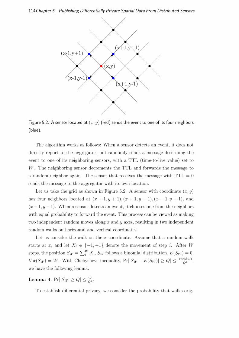
114Chapter 5. Publishing Differentially Private Spatial Data From Distributed Sensors
(x,y)
(x+1,y+1)
(x+1,y-1)
(x-1,y+1)
(x-1,y-1)
Figure 5.2: A sensor located at (x, y) (red) sends the event to one of its four neighbors
(blue).
The algorithm works as follows: When a sensor detects an event, it does not
directly report to the aggregator, but randomly sends a message describing the
event to one of its neighboring sensors, with a TTL (time-to-live value) set to
W . The neighboring sensor decrements the TTL and forwards the message to
a random neighbor again. The sensor that receives the message with TTL = 0
sends the message to the aggregator with its own location.
Let us take the grid as shown in Figure 5.2. A sensor with coordinate (x, y)
has four neighbors located at (x + 1, y + 1), (x + 1, y − 1), (x − 1, y + 1), and
(x− 1, y− 1). When a sensor detects an event, it chooses one from the neighbors
with equal probability to forward the event. This process can be viewed as making
two independent random moves along x and y axes, resulting in two independent
random walks on horizontal and vertical coordinates.
Let us consider the walk on the x coordinate. Assume that a random walk
starts at x, and let Xi ∈ {−1,+1} denote the movement of step i. After W
steps, the position SW =∑W
1 Xi, SW follows a binomial distribution, E(SW ) = 0,
Var(SW ) = W . With Chebyshevs inequality, Pr[|SW − E(SW )| ≥ Q] ≤ Var(SW )Q2 ,
we have the following lemma.
Lemma 4. Pr[|SW | ≥ Q] ≤ WQ2 .
To establish differential privacy, we consider the probability that walks orig-
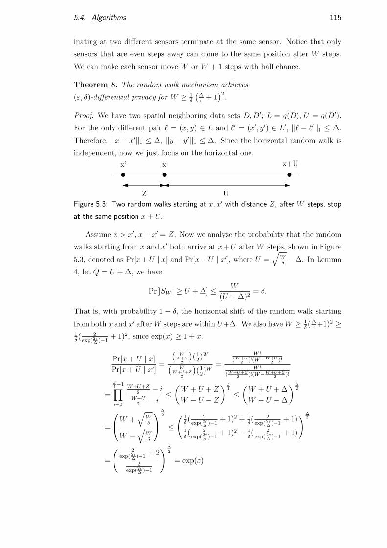
5.4. Algorithms 115
inating at two different sensors terminate at the same sensor. Notice that only
sensors that are even steps away can come to the same position after W steps.
We can make each sensor move W or W + 1 steps with half chance.
Theorem 8. The random walk mechanism achieves
(ε, δ)-differential privacy for W ≥ 1δ
(∆ε
+ 1)2
.
Proof. We have two spatial neighboring data sets D,D′; L = g(D), L′ = g(D′).
For the only different pair ` = (x, y) ∈ L and `′ = (x′, y′) ∈ L′, ||` − `′||1 ≤ ∆.
Therefore, ||x − x′||1 ≤ ∆, ||y − y′||1 ≤ ∆. Since the horizontal random walk is
independent, now we just focus on the horizontal one.
xx’ x+U
Z U
Figure 5.3: Two random walks starting at x, x′ with distance Z, after W steps, stop
at the same position x+ U .
Assume x > x′, x− x′ = Z. Now we analyze the probability that the random
walks starting from x and x′ both arrive at x+U after W steps, shown in Figure
5.3, denoted as Pr[x+U | x] and Pr[x+U | x′], where U =√
Wδ−∆. In Lemma
4, let Q = U + ∆, we have
Pr[|SW | ≥ U + ∆] ≤ W
(U + ∆)2= δ.
That is, with probability 1− δ, the horizontal shift of the random walk starting
from both x and x′ after W steps are within U+∆. We also have W ≥ 1δ(∆ε
+1)2 ≥1δ( 2
exp( 2ε∆
)−1+ 1)2, since exp(x) ≥ 1 + x.
Pr[x+ U | x]
Pr[x+ U | x′]=
(W
W+U2
)(1
2)W(
WW+U+Z
2
)(1
2)W
=
W !(W+U
2)!(W−W+U
2)!
W !(W+U+Z
2)!(W−W+U+Z
2)!
=
Z2−1∏i=0
W+U+Z2− i
W−U2− i
≤(W + U + Z
W − U − Z
)Z2
≤(W + U + ∆
W − U −∆
)∆2
=
W +√
Wδ
W −√
Wδ
∆2
≤
( 1δ( 2
exp( 2ε∆
)−1+ 1)2 + 1
δ( 2
exp( 2ε∆
)−1+ 1)
1δ( 2
exp( 2ε∆
)−1+ 1)2 − 1
δ( 2
exp( 2ε∆
)−1+ 1)
)∆2
=
( 2exp( 2ε
∆)−1
+ 2
2exp( 2ε
∆)−1
)∆2
= exp(ε)

116Chapter 5. Publishing Differentially Private Spatial Data From Distributed Sensors
Therefore, the random walk mechanism in one dimension achieves (ε, δ)-
differential privacy. Since the random walk on horizontal and vertical directions
are independent, we conclude that the random walk on two dimension grids also
achieves (ε, δ)-differential privacy.
The following lemma shows that the displacement to an event’s location due
to the random walk is bounded, and therefore, the spatial perturbation process
does not significantly change the event distribution.
Lemma 5. When achieving (ε, δ)-differential privacy, with probability 1−δ, after
W steps, the Euclidean distance between the sensor reporting to the message and
the original sensor detecting the event is at most√
2δ
(∆ε
+ 1).
Proof. In the proof of theorem 8, for the random walk on one dimension, if
W ≥ 1δ
(∆ε
+ 1)2
, we have |SW | satisfies,
|SW | ≤√W
δ≤ 1
δ
(∆
ε+ 1
).
Therefore, the euclidean distance for the random walk in two dimension is at
most√
2δ
(∆ε
+ 1).
The random walk mechanism, in addition to perturbing the events to a suit-
able distribution, has additional privacy properties. In Scenarios where an adver-
sary can sense transmissions from sensors, such random walks generated by many
sensors can help to obscure the source of events, particularly when mixed with ac-
tivities of fake events described in the next section. Such mixing methods are used
in the TOR network and known to effectively obscure message sources(Piotrowska
et al., 2017).
The results for homogeneous temporal and spatial Poisson processes in this
section can be applied to non-homogeneous Poisson processes by changing the
sensitivity according to the intensity function, and operating according to the
local intensity value.
5.4.2 Poisson Process for Event Privacy
For the setting where the sensors can not trust each other, the above method
do not apply. Here, we model the real event sequence by a non-homogeneous
5.4. Algorithms 117
Poisson process with spatial intensity function λ(Σ), where Σ are the parameters
for space. This model closely relate to the privacy preserving method presented
in Section 3.5.2. Events there follow a non-homogeneous Poisson process with a
one dimensional intensity function.
To protect the occurrence of a single event using differential privacy, the fol-
lowing algorithm, AD(R), is designed. Here, D is the input dataset and R ⊆ R2
denotes the domain range. Augment D with N ′ fake events uniformly distributed
over the domain where N ′ follows a Poisson distribution with intensity function
λ(Σ). Then given a range R, the algorithm AD(R) outputs the total number of
events (real and fake) inside the range, R.
We first prove that the above algorithm satisfies differential privacy.
Theorem 9. AD(R) is (ε, δ)-differentially private, when Λ = O(
1ε2
log 1δ
), where
Λ denotes the integrated intensity over the range, R, i.e., Λ =∫Rλ(s)ds.
Proof. For simplicity of the proof, let’s consider one dimensional data along real
line R. Note that the below argument hold for two dimensional space as the Pois-
son process is trivially extended to two dimension considering a two dimensional
intensity function.
Consider two neighboring datasets D and D′ (one dimensional data). Without
loss of generality, assume that D has one additional event at τ . Now, any query
range not containing τ have the same probability for all the outputs given the
input datasets D and D′.
Now, consider a query interval, I, containing τ . To have the same outputs
given input D and D′, AD′ need to introduce one more fake event than AD.
Therefore,
Pr[AD(I) = N ]
Pr[AD′(I) = N ]=
exp(−Λ (Λ)N
′
N ′!
)exp
(−Λ (Λ)N′+1
(N ′+1)!
) =Λ
N ′ + 1,
where N ′ is the number of fake events introduced by AD.
Let’s partition the range of the values of N ′, into two parts N1 and N2.
Let, N1 = {x ∈ N| |Λ− x| ≤ Λ(1 − e−ε) + 1} and N2 = {x ∈ N| |Λ− x| >Λ(1− e−ε) + 1}.
Let α = Λ(1− e−ε) + 1. For N ′ ∈ N2, using Lemma 1 we have,
118Chapter 5. Publishing Differentially Private Spatial Data From Distributed Sensors
Pr[|N ′ − Λ| ≥ α] ≤ 2 exp
(− α2
2(Λ + α)
)=2 exp
(− (Λ(1− e−ε) + 1)2
2(Λ(2− e−ε) + 1)
)≤ 2 exp
(−Λ(1− e−ε)2
2(2− e−ε)
)≤ δ,
where Λ =2(2−e−ε) log 2
δ
(1−e−ε)2 , which is O( 1ε2
log 1δ) when ε is small.
For N ′ ∈ N1, we have
Pr[AD(I) = N ]
Pr[A′D(I) = N ]=
Λ
N ′ + 1≤ Λ
Λe−ε − 1 + 1= eε.
Therefore, combining above equations we have,
Pr[AD(I) = N ] = Pr[N ′ ∈ R1] + Pr[N ′ ∈ R2]
≤ eε Pr[AD′(I) = N ] + δ
Publishing data. The above sanitization algorithm AD(R) can be considered
for publishing data; If one considers query for all possible intervals it is equivalent
to publishing the events. Practically, each sensor can publish the union of the
real and fake events and the published data would preserve differential privacy
as argued above.
Answering Range Queries. Now, we design an algorithm, Q(AD(R)), to
accurately answer range queries based on the results published by AD(R). As in
the most security and privacy settings where the algorithms and their parameters
are all public except the specific random choices the algorithms make, consider
ε, δ, and the event intensity λ are known.
Counting query on a spatial range R = [x1, x2] × [y1, y2] is estimated as
AD(R) − Λ, where Λ =∫ x2
x1
∫ y2
y1λ(s)ds. Let’s denote AD(R) as n for simplic-
ity.
Let’s denote the count of real events inside the range R in the dataset D as n∗.
Now, n∗− n gives an unbiased estimator for n∗, by the well known superposition
theorem. We present the main statement below.
Theorem 10. Superposition Theorem (Kingman, 1992; Grimmett and
Stirzaker, 2001). The superposition of independent Poisson point processes
N1, N2, · · · , Nm with mean rates Λ1,Λ2, · · · ,Λm respectively is a Poisson point
process with mean rate of Λ =∑m
i=1 Λi.
5.4. Algorithms 119
Now we analyze the utility of our algorithm.
Lemma 6. The algorithm QS, for a probability 0 ≤ β ≤ 1, gives the following
range query error
Pr
[|QS(A(R))− n∗| ≤ log
2
β+
√log2 2
β+ 2Λ log
2
β
]≥ 1− β.
Proof. Notice that QS(A(R)) is n − Λ. The count of fake events, n − n∗, fol-
lows the Poisson distribution with mean Λ. Therefore, applying α ≥ log 2β
+√log2 2
β+ 2Λ log 2
βin Lemma 1, we have 2 exp
(− α2
2(Λ+α)
)≤ β. Therefore,
Pr
[|n− Λ− n∗| ≥ log
2
β+
√log2 2
β+ 2Λ log
2
β
]≤ β.
Rearranging we get the lemma.
Theorem 11. If Λ = O(
1ε2
log 1δ
), QD(A(R)) estimates the counts of real events
with error O(√
1ε2
log 1δ
log 1β
), with probability 1− β.
Replacing the value of Λ in the above Lemma gives the theorem.
Extension to spatiotemporal data. Poisson process is trivially extended to
spatiotemporal dimension by using suitable intensity function in three dimen-
sions. The spatiotemporal sanitization mechanism can generate fake events to
obfuscate both the accurate location and timing. This method is suitable for
realtime data analysis.
5.4.3 Extending Psum Method to Spatial Dimension
Here, we extend the results from (Chan et al., 2011) designed for temporal queries
to spatial dimension and we compare its accuracy with our algorithms in the
experiments.
Let’s assume that the sensors are positioned on a√m×√m unit square grid.
An event occurring at location (x, y) is recorded by the sensor nearest to (x, y); for
multiple nearest sensors we choose one arbitrarily. Suppose, S(x, y) ∈ N denotes
the number of events recorded by the sensor at grid location (x, y).
To protect the presence of a single event in the dataset, differential privacy
considers neighboring dataset S and S ′ that have event count differing by 1 at
one sensor.

120Chapter 5. Publishing Differentially Private Spatial Data From Distributed Sensors
Similar to the binary mechanism in (Chan et al., 2011), a quadtree (Samet,
1988) can be constructed over S and any range query can be answered by adding
the canonical ranges of the query range; Let’s call these sums as partial sums.
Thus, a change in a cell S(x, y) affects at most dlog2me queries.
The randomized mechanism A adds Laplace noise with b = logm/ε to each
partial sum. We now analyze the privacy and utility of this mechanism.
Theorem 12 (Differential privacy). The above mechanism preserves ε-
differential privacy.
Proof. It is easy to see that for a single query, the above mechanism preservesε
logm-differential privacy. As there can be at most dlogme queries affected by this
change, sequential composition of the differential privacy gives the theorem.
Before analyzing the utility of the method, we need the following lemma
Theorem 13 (Utility). For a spatiotemporal range query, the error of the above
mechanism is O(
log1.52 m
εlog 1
β
)with probability 1− β.
Proof. Corresponding to noises at partial sums, a query accumulates total noise
from dlog2me Laplace distributions each with bi = logm/ε. This gives the theo-
rem.
5.5 Experiments
This section describes experiments showing that the privacy preserving mecha-
nisms for the proposed algorithms. Highlights of the results are
• Proposed methods are more accurate for range queries than existing con-
tinual release methods for same privacy guarantees.
• Privacy preserving mechanisms work in real datasets of geo-located tweets.
5.5.1 Experimental Setup
Dataset. We use a publicly available dataset of 9, 267 Geo-located tweets from
London, UK1.
Evaluating utility using range queries. Range queries are fundamental to
mining and learning methods and thus used here as the measure of utility of the
1http://followthehashtag.com/datasets/170000-uk-geolocated-tweets-free-twitter-dataset/
5.5. Experiments 121
sanitized data. Each experiment uses 5000 uniformly chosen query ranges and
the experiments are repeated 10 times to capture confidence in the result. If the
count of events in a query range with n events is estimated as n, then the error in
estimation is ξ = |n−n|n
. The relative error is symmetric with respect to addition,
i.e., estimating n+ ∆ and n−∆ incur same error.
5.5.2 Evaluating Random walk based algorithm
This subsection evaluates the mechanisms proposed in Section 5.4.1 for publishing
spatial events.
Accuracy for spatial range queries. Figure 5.4(a), (b), and (c) show how
relative error changes for spatial range queries on the spatial data publish model.
The range queries are accurate for reasonable privacy, i.e., with large ∆ and small
ε and δ values.
5.5.3 Evaluating Poisson Process based algorithm
This section describes experiments corresponding to methods proposed in Sec-
tion 5.4.2.
In this setting, the the space is divided into cubic grid cells indexed by (x, y)
with spatial resolution as 50 meters. Each event is mapped to its nearest grid
point and the intensity of the fake events at each cell is determined using Theo-
rem 9. The events are sanitized using the mechanism described in Section 5.4.2.
Relative error, ξ increases with increasing privacy as shown in Figure 5.5(a) and
(b) by varying ε and δ.
Spatial privacy for synchronous model. This section evaluates range queries
in synchronous setting described in 5.4.3. The space-time is divided into a gird,
with the spatial resolution being 50 meters. A quadtree is built on this grid and
a query is answered by aggregating counts of the partial canonical ranges.
Compare utility of methods. In Figure 5.6, we notice that the spatial partial
sum method achieves lowest error for range queries compared to privacy preserv-
ing mechanism with Poisson process method and naive Laplace perturbation.
The naive Laplace perturbation algorithm first computes the accurate answer to
the range query and then adds Lap(m)/ε noise in a domain with√m×√m grid.
Also note that neither the naive Laplace mechanism nor the partial sum method
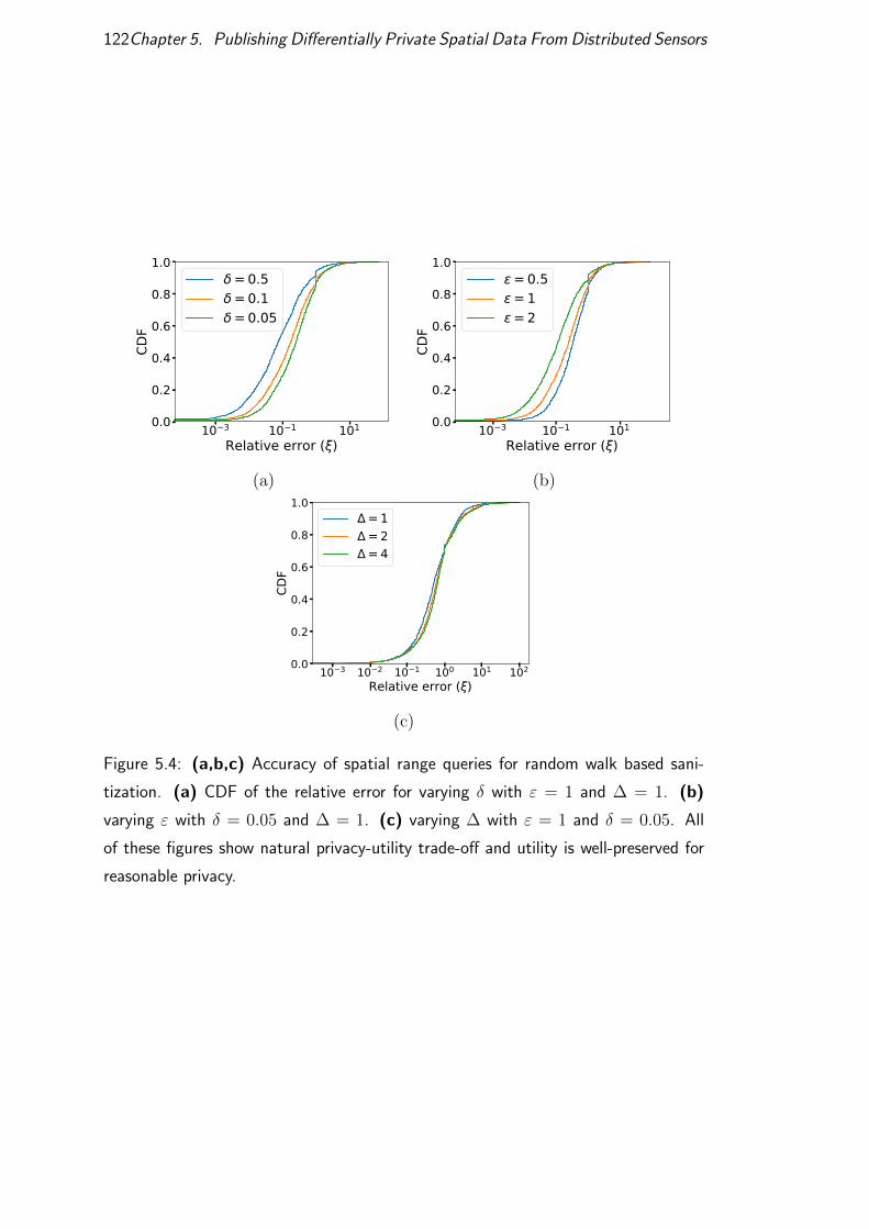
122Chapter 5. Publishing Differentially Private Spatial Data From Distributed Sensors
10 3 10 1 101
Relative error ( )0.0
0.2
0.4
0.6
0.8
1.0
CDF
= 0.5= 0.1= 0.05
10 3 10 1 101
Relative error ( )0.0
0.2
0.4
0.6
0.8
1.0
CDF
= 0.5= 1= 2
(a) (b)
10 3 10 2 10 1 100 101 102
Relative error ( )0.0
0.2
0.4
0.6
0.8
1.0
CDF
= 1= 2= 4
(c)
Figure 5.4: (a,b,c) Accuracy of spatial range queries for random walk based sani-
tization. (a) CDF of the relative error for varying δ with ε = 1 and ∆ = 1. (b)
varying ε with δ = 0.05 and ∆ = 1. (c) varying ∆ with ε = 1 and δ = 0.05. All
of these figures show natural privacy-utility trade-off and utility is well-preserved for
reasonable privacy.
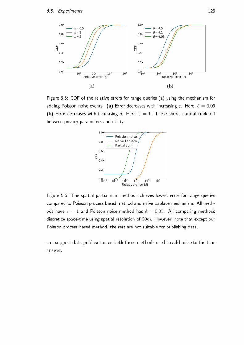
5.5. Experiments 123
101 102 103 104
Relative error ( )0.0
0.2
0.4
0.6
0.8
1.0
CDF
= 0.5= 1= 2
100 101 102 103
Relative error ( )0.0
0.2
0.4
0.6
0.8
1.0
CDF
= 0.5= 0.1= 0.05
(a) (b)
Figure 5.5: CDF of the relative errors for range queries (a) using the mechanism for
adding Poisson noise events. (a) Error decreases with increasing ε. Here, δ = 0.05
(b) Error decreases with increasing δ. Here, ε = 1. These shows natural trade-off
between privacy parameters and utility.
10 5 10 3 10 1 101 103 105
Relative error ( )0.0
0.2
0.4
0.6
0.8
1.0
CDF
Poission noiseNaive LaplacePartial sum
Figure 5.6: The spatial partial sum method achieves lowest error for range queries
compared to Poisson process based method and naive Laplace mechanism. All meth-
ods have ε = 1 and Poisson noise method has δ = 0.05. All comparing methods
discretize space-time using spatial resolution of 50m. However, note that except our
Poisson process based method, the rest are not suitable for publishing data.
can support data publication as both these methods need to add noise to the true
answer.

Chapter 6
Conclusion and Future Directions
Sensing using IoT devices and mobile phones have proliferated in pervasive areas
of modern day living (Gubbi et al., 2013). Fundamental learning techniques such
as the ones proposed in this dissertation will be of interest for years to come.
In this dissertation, we present multiple learning algorithms for spatiotemporal
sensing data. The algorithms are efficient with online and distributed computa-
tion. They preserve individual privacy and learn aggregate knowledge from the
data. This chapter presents the concluding remarks and brief ideas on related
open research areas.
Learning periodicity from noisy streams. We have demonstrated the use of
a sequential Monte Carlo method to detect and track the periodicity in discrete
event streams. Unlike other methods, this technique does not rely on the under-
lying process sticking to a constant phase. As a result, it adapts to noise and
changes in the period very quickly. Experiments show this method to be more
accurate and efficient than existing methods for detecting periodicity in noisy
event streams.
Our basic approach is quite general and can be adapted to detect and char-
acterize more complex temporal patterns. Doing so will require a more flexible
class of event-generating functions, which we expect will be a fruitful area for
future research.
Many applications require inference from an aggregate signal contributed by
multiple periodic signals. Examples include forecasting demand for an item (e.g.,
shampoo) at a super market. Many users buy shampoos at regular intervals,
although their phases and intervals are dynamic. It is interesting and as well as
challenging to analyze the interweaving pattern in the data. Frequency analysis
125
126 Chapter 6. Conclusion and Future Directions
techniques are not applicable due to dynamic phases and periodicity in each sig-
nal; Markov models become complicated for high dimensional data. It is possible
to treat the signal as a univariate signal of demands and apply regression tech-
niques, but that misses the structure provided by the periodicity in individual
user’s buying patterns.
Chapter 2 empirically shows that the algorithm works in real and artificial
data, but a rigorous mathematical analysis would be required to characterize
the algorithm, for example, lower bound of the number of events required for
convergence, the number of particles needed for robust operation, etc.
Private Sensing of Asynchronous Event Sequences. In Chapter 3, we
proposed multiple privacy preserving mechanisms for protecting individual event
timings and hiding the occurrence of an event. The proposed framework uses con-
temporary Pufferfish definition of privacy – a generalization of differential privacy
– and supports asynchronous event timings. The mechanisms add considerably
less noise than the existing algorithms to achieve the same privacy guarantee.
We also proposed a system design to implement the framework in mobile phones.
Multivariate event streams that carry interrelations are harder to sanitize as they
may contain a complex relation between attributes, and this remains to be inves-
tigated in future works.
Topological Signatures For Fast Mobility Analysis. In Chapter 4, We pre-
sented a topological framework to represent a trajectory as a point in a Euclidean
space, enabling natural applications of well established machine learning and min-
ing techniques. The topological construct preserves relevant qualitative features
in trajectories while ignoring the extraneous details and noise. The framework
can be set up using fast distributed algorithms and used in an online manner
by mobile entities. The framework is quite general and flexible, and it allows
application specific choice of obstacles and domains.
The proposed framework uses the obstacles and designs a method to infer
obstacles from trajectory data (no or less mobility correspond to obstacles), how-
ever, further study is needed to characterize the obstacles in a domain. This
would provide insight to causality behind mobility (Cobb et al., 2017).
Many applications like driver-less cars need to consider dynamic obstacles
(other vehicles and pedestrians on road). Our framework does not trivially extend
to dynamic obstacles and needs further work.
127
Time is an essential attribute in mobility traces for many applications. How-
ever, it is nontrivial to extend our framework to the temporal dimension because
of the uni-direction property of time (Ghrist and Krishnan, 2017). Therefore, it
needs further study to analyze spatiotemporal trajectories using topology.
Publishing Differentially Private Spatial Data From Distributed Sen-
sors. In Chapter 5, we proposed a differentially private sensing framework for
spatial data publication. The proposed framework supports distributed operation
and has good privacy and utility guarantees for independent events. However,
in many applications, spatial events are correlated, for example, occupancy re-
lates to mobility and locations in a trajectory, etc. Due to the correlation in the
data, traditional differential privacy frameworks do not apply and therefore, need
further investigation.
Moreover, the algorithms in this chapter apply to axis aligned rectangular
queries where sensors are arranged on a grid. Further study is required to support
more realistic general graph topology and general shaped ranges.

Bibliography
(2017). Mdanalysis 0.16.2. http://www.mdanalysis.org/.
Abadi, M., Barham, P., Chen, J., Chen, Z., Davis, A., Dean, J., Devin, M.,
Ghemawat, S., Irving, G., Isard, M., et al. (2016). Tensorflow: A system for
large-scale machine learning. In OSDI, volume 16, pages 265–283.
Ahmadi, H., Pham, N. T., Ganti, R. K., Abdelzaher, T. F., Nath, S., and Han,
J. (2010). Privacy-aware regression modeling of participatory sensing data. In
SenSys.
Alt, H. and Godau, M. (1995). Computing the frechet distance between two
polygonal curves. International Journal of Computational Geometry & Appli-
cations, 5(01n02):75–91.
Andres, M. E., Bordenabe, N. E., Chatzikokolakis, K., and Palamidessi, C.
(2013). Geo-indistinguishability: Differential privacy for location-based sys-
tems. In Proceedings of the 2013 ACM SIGSAC Conference on Computer &
Communications Security, CCS ’13, pages 901–914. ACM.
Astefanoaei, M., Cesaretti, P., Katsikouli, P., Goswami, M., and Sarkar, R.
(2018). Multi-resolution sketches and locality sensitive hashing for fast tra-
jectory processing. In 26th ACM SIGSPATIAL International Conference on
Advances in Geographic Information Systems (ACM SIGSPATIAL).
Bachem, O., Lucic, M., and Krause, A. (2017). Scalable and distributed clustering
via lightweight coresets. arXiv preprint arXiv:1702.08248.
Bao, L. and Intille, S. S. (2004). Activity recognition from user-annotated accel-
eration data. In International conference on pervasive computing, pages 1–17.
Springer.
129
130 Bibliography
Barbosa, H., Barthelemy, M., Ghoshal, G., James, C. R., Lenormand, M., Louail,
T., Menezes, R., Ramasco, J. J., Simini, F., and Tomasini, M. (2018). Human
mobility: Models and applications. Physics Reports, 734:1–74.
Barth, J., Klucken, J., Kugler, P., Kammerer, T., Steidl, R., Winkler, J., Horneg-
ger, J., and Eskofier, B. (2011). Biometric and mobile gait analysis for early
diagnosis and therapy monitoring in parkinson’s disease. In Engineering in
Medicine and Biology Society, EMBC, 2011 Annual International Conference
of the IEEE, pages 868–871. IEEE.
Baryshnikov, Y. and Ghrist, R. (2009). Target enumeration via euler character-
istic integrals. SIAM Journal on Applied Mathematics, 70(3):825–844.
Benson, T., Akella, A., and Maltz, D. A. (2010). Network traffic characteristics of
data centers in the wild. In Proceedings of the 10th ACM SIGCOMM conference
on Internet measurement, pages 267–280. ACM.
Bindschaedler, V. and Shokri, R. (2016). Synthesizing plausible privacy-
preserving location traces. In 2016 IEEE Symposium on Security and Privacy
(SP), pages 546–563. IEEE.
Bittau, A., Erlingsson, U., Maniatis, P., Mironov, I., Raghunathan, A., Lie, D.,
Rudominer, M., Kode, U., Tinnes, J., and Seefeld, B. (2017). Prochlo: Strong
privacy for analytics in the crowd. In Proceedings of the 26th Symposium on
Operating Systems Principles, pages 441–459. ACM.
Bracciale, L., Bonola, M., Loreti, P., Bianchi, G., Amici, R., and Rabuffi, A.
(2014). Crawdad data set roma/taxi (v. 2014-07-17). July.
Buchin, K., Buchin, M., Gudmundsson, J., Loffler, M., and Luo, J. (2011). De-
tecting commuting patterns by clustering subtrajectories. International Jour-
nal of Computational Geometry & Applications, 21(03):253–282.
Buchin, K., Buchin, M., Van Kreveld, M., Loffler, M., Silveira, R. I., Wenk, C.,
and Wiratma, L. (2013). Median trajectories. Algorithmica, 66(3):595–614.
Candes, E. (2006). Compressive sampling.
Canini, K. R., Shi, L., and Griffiths, T. L. (2009). Online inference of topics with
latent dirichlet allocation. In International conference on artificial intelligence
and statistics, pages 65–72.
Bibliography 131
Cao, L. and Krumm, J. (2009). From gps traces to a routable road map. In Pro-
ceedings of the 17th ACM SIGSPATIAL international conference on advances
in geographic information systems, pages 3–12. ACM.
Cao, Y., Yoshikawa, M., Xiao, Y., and Xiong, L. (2018). Quantifying differ-
ential privacy in continuous data release under temporal correlations. IEEE
Transactions on Knowledge and Data Engineering.
Chambers, E. W., De Verdiere, E. C., Erickson, J., Lazard, S., Lazarus, F., and
Thite, S. (2010). Homotopic frechet distance between curves or, walking your
dog in the woods in polynomial time. Computational Geometry, 43(3):295–311.
Chambers, E. W. and Wang, Y. (2013). Measuring similarity between curves
on 2-manifolds via homotopy area. In Proceedings of the twenty-ninth annual
symposium on Computational geometry, pages 425–434. ACM.
Chan, T.-H. H., Shi, E., and Song, D. (2011). Private and continual release of
statistics. ACM Trans. Inf. Syst. Secur., 14(3):26:1–26:24.
Chen, Y., Machanavajjhala, A., Hay, M., and Miklau, G. (2017). Pegasus: Data-
adaptive differentially private stream processing. In Proceedings of the 2017
ACM SIGSAC Conference on Computer and Communications Security, pages
1375–1388. ACM.
Cheng, C.-M., Kung, H., and Tan, K.-S. (2002). Use of spectral analysis in
defense against dos attacks. In Global Telecommunications Conference, 2002.
GLOBECOM’02. IEEE, volume 3, pages 2143–2148. IEEE.
Cobb, A. D., Markham, A., and Roberts, S. J. (2017). Learning from li-
ons: inferring the utility of agents from their trajectories. arXiv preprint
arXiv:1709.02357.
Cormode, G., Procopiuc, C., Srivastava, D., Shen, E., and Yu, T. (2012). Dif-
ferentially private spatial decompositions. In Data engineering (ICDE), 2012
IEEE 28th international conference on, pages 20–31. IEEE.
Datar, M., Immorlica, N., Indyk, P., and Mirrokni, V. S. (2004). Locality-sensitive
hashing scheme based on p-stable distributions. In Proceedings of the twentieth
annual symposium on Computational geometry, pages 253–262. ACM.
132 Bibliography
De Montjoye, Y.-A., Hidalgo, C. A., Verleysen, M., and Blondel, V. D. (2013).
Unique in the crowd: The privacy bounds of human mobility. Scientific reports,
3:1376.
Desbrun, M., Kanso, E., and Tong, Y. (2008). Discrete differential forms for com-
putational modeling. In Discrete differential geometry, pages 287–324. Springer.
Diederik P. Kingma, J. B. (2015). Adam: A method for stochastic optimization.
In Proceedings of the 3rd International Conference on Learning Representations
(ICLR), ICLR ’15.
Ding, J., Gao, J., and Xiong, H. (2015). Understanding and modelling informa-
tion dissemination patterns in vehicle-to-vehicle networks. In Proceedings of
the 23rd SIGSPATIAL International Conference on Advances in Geographic
Information Systems, page 41. ACM.
Ding, J., Ghosh, A., Sarkar, R., and Gao, J. (2019). Private sensing of asyn-
chronous event sequences. In Under Review at Sensys 2019.
Doucet, A., Freitas, N. d., and Gordon, N., editors (2001). Sequential Monte
Carlo Methods in Practice. Springer, New York.
Driemel, A. and Silvestri, F. (2017). Locality-Sensitive Hashing of Curves. In
33rd International Symposium on Computational Geometry (SoCG 2017), vol-
ume 77, pages 37:1–37:16.
Dwork, C. (2006). Differential privacy. In Proceedings of the 33rd Interna-
tional Conference on Automata, Languages and Programming - Volume Part
II, ICALP’06, pages 1–12. Springer-Verlag.
Dwork, C., McSherry, F., Nissim, K., and Smith, A. (2006). Calibrating noise
to sensitivity in private data analysis. In Theory of cryptography conference,
pages 265–284. Springer.
Dwork, C., Naor, M., Pitassi, T., and Rothblum, G. N. (2010). Differential
privacy under continual observation. In Proceedings of the forty-second ACM
symposium on Theory of computing, pages 715–724. ACM.
Dwork, C., Naor, M., Reingold, O., and Rothblum, G. N. (2015). Pure differential
privacy for rectangle queries via private partitions. In International Conference
Bibliography 133
on the Theory and Application of Cryptology and Information Security, pages
735–751. Springer.
Dwork, C., Naor, M., Reingold, O., Rothblum, G. N., and Vadhan, S. (2009). On
the complexity of differentially private data release: Efficient algorithms and
hardness results. In Proceedings of the Forty-first Annual ACM Symposium on
Theory of Computing, STOC ’09, pages 381–390, New York, NY, USA. ACM.
Dwork, C. and Roth, A. (2014). The algorithmic foundations of differential pri-
vacy. Found. Trends Theor. Comput. Sci., 9(3–4):211–407.
Easley, D. and Kleinberg, J. (2010). Networks, crowds, and markets: Reasoning
about a highly connected world. Cambridge University Press.
Edelsbrunner, H. and Harer, J. (2010). Computational topology: an introduction.
American Mathematical Soc.
Elmokashfi, A., Zhou, D., and Baltrunas, D. (2017). Adding the next nine: An
investigation of mobile broadband networks availability. In Proceedings of the
23rd Annual International Conference on Mobile Computing and Networking,
pages 88–100. ACM.
Erlingsson, U., Pihur, V., and Korolova, A. (2014). Rappor: Randomized aggre-
gatable privacy-preserving ordinal response. In Proceedings of the 2014 ACM
SIGSAC conference on computer and communications security, pages 1054–
1067. ACM.
Fan, L., Xiong, L., and Sunderam, V. (2013). Differentially private multi-
dimensional time series release for traffic monitoring. In IFIP Annual Con-
ference on Data and Applications Security and Privacy, pages 33–48. Springer.
Frahling, G. and Sohler, C. (2008). A fast k-means implementation using coresets.
International Journal of Computational Geometry & Applications, 18(06):605–
625.
Funke, S. and Milosavljevic, N. (2007). Network sketching or: How much ge-
ometry hides in connectivity?–part ii. In Proceedings of the eighteenth annual
ACM-SIAM symposium on Discrete algorithms, pages 958–967. Society for In-
dustrial and Applied Mathematics.
134 Bibliography
Ganti, R. K., Pham, N., Tsai, Y.-E., and Abdelzaher, T. F. (2008). Poolview:
stream privacy for grassroots participatory sensing. In Proceedings of the 6th
ACM conference on Embedded network sensor systems, pages 281–294. acm.
Gers, F. A., Schmidhuber, J., and Cummins, F. A. (2000). Learning to forget:
Continual prediction with lstm. Neural Computation, 12:2451–2471.
Ghassemi, N. H. and Diesenroth, M. (2014). Analytic long term forecasting with
periodic gaussian processes. In AISTATS, pages 303–311.
Ghosh, A., Ding, J., Sarkar, R., and Gao, J. (2019). Differentially private sensing
of distributed spatial data. In Working for submission.
Ghosh, A., Lucas, C., and Sarkar, R. (2017). Finding periodic discrete events in
noisy streams. In Proceedings of the 2017 ACM on Conference on Information
and Knowledge Management, pages 627–636. ACM.
Ghosh, A., Rozemberczki, B., Ramamoorthy, S., and Sarkar, R. (2018). Topo-
logical signatures for fast mobility analysis. In Proceedings of the 26th ACM
SIGSPATIAL International Conference on Advances in Geographic Informa-
tion Systems, pages 159–168. ACM.
Ghrist, R. and Krishnan, S. (2017). Positive alexander duality for pursuit and
evasion.
Goldberg, Y. (2017). Neural network methods for natural language processing.
Synthesis Lectures on Human Language Technologies, 10(1):1–309.
Goldreich, O. (2017). Introduction to property testing. Cambridge University
Press.
Gonzalez, M. C., Hidalgo, C. A., and Barabasi, A.-L. (2009). Understanding
individual human mobility patterns. Nature, 458(7235):238–238.
Gramaglia, M. and Fiore, M. (2015). Hiding mobile traffic fingerprints with
glove. In Proceedings of the 11th ACM Conference on Emerging Networking
Experiments and Technologies, page 26. ACM.
Gramaglia, M., Fiore, M., Tarable, A., and Banchs, A. (2017). Preserving mobile
subscriber privacy in open datasets of spatiotemporal trajectories. In IEEE
Bibliography 135
INFOCOM 2017-IEEE Conference on Computer Communications, pages 1–9.
IEEE.
Grimmett, G. and Stirzaker, D. (2001). Probability and random processes. Oxford
university press.
Gubbi, J., Buyya, R., Marusic, S., and Palaniswami, M. (2013). Internet of
things (iot): A vision, architectural elements, and future directions. Future
Generation Comp. Syst., 29:1645–1660.
HajiGhassemi, N. and Deisenroth, M. (2014). Analytic long-term forecasting
with periodic gaussian processes. In Artificial Intelligence and Statistics, pages
303–311.
Hallac, D., Vare, S., Boyd, S., and Leskovec, J. (2017). Toeplitz inverse
covariance-based clustering of multivariate time series data. In Proceedings
of the 23rd ACM SIGKDD International Conference on Knowledge Discovery
and Data Mining, pages 215–223. ACM.
Han, J., Dong, G., and Yin, Y. (1999). Efficient mining of partial periodic pat-
terns in time series database. In Data Engineering, 1999. Proceedings., 15th
International Conference on, pages 106–115. IEEE.
He, X., Machanavajjhala, A., and Ding, B. (2014). Blowfish privacy: tuning
privacy-utility trade-offs using policies. In SIGMOD Conference.
Hershberger, J. and Snoeyink, J. (1994a). Computing minimum length paths of
a given homotopy class. Computational geometry, 4(2):63–97.
Hershberger, J. and Snoeyink, J. (1994b). An o(n log n) implementation of the
douglas-peucker algorithm for line simplification. In Symposium on Computa-
tional Geometry.
Hirani, A. N. (2003). Discrete exterior calculus. PhD thesis, California Institute
of Technology.
Indyk, P. (2002). Approximate nearest neighbor algorithms for frechet distance
via product metrics. In Proceedings of the eighteenth annual symposium on
Computational geometry, pages 102–106. ACM.
136 Bibliography
Indyk, P., Koudas, N., and Muthukrishnan, S. (2000). Identifying representative
trends in massive time series data sets using sketches. In VLDB, pages 363–372.
Jain, M. and Dovrolis, C. (2002). End-to-end available bandwidth: Measurement
methodology, dynamics, and relation with TCP throughput, volume 32. ACM.
Jia, X., Khandelwal, A., Nayak, G., Gerber, J., Carlson, K., West, P., and Ku-
mar, V. (2017). Incremental dual-memory lstm in land cover prediction. In
Proceedings of the 23rd ACM SIGKDD International Conference on Knowledge
Discovery and Data Mining, pages 867–876. ACM.
Jin, H., Su, L., Xiao, H., and Nahrstedt, K. (2016). Inception: Incentivizing
privacy-preserving data aggregation for mobile crowd sensing systems. In Pro-
ceedings of the 17th ACM International Symposium on Mobile Ad Hoc Net-
working and Computing, pages 341–350. ACM.
Jindal, T., Giridhar, P., Tang, L.-A., Li, J., and Han, J. (2013). Spatiotempo-
ral periodical pattern mining in traffic data. In Proceedings of the 2nd ACM
SIGKDD International Workshop on Urban Computing, page 11. ACM.
Junier, I., Herisson, J., and Kepes, F. (2010). Periodic pattern detection in sparse
boolean sequences. Algorithms for Molecular Biology, 5(1):1.
Jurafsky, D. and Martin, J. H. (2014). Speech and language processing, volume 3.
Pearson London.
Kasiviswanathan, S. P., Lee, H. K., Nissim, K., Raskhodnikova, S., and Smith, A.
(2011). What can we learn privately? SIAM Journal on Computing, 40(3):793–
826.
Katsikouli, P., Astefanoaei, M., and Sarkar, R. (2018). Distributed mining of
popular paths in road networks. In DCOSS 2018-International Conference on
Distributed Computing in Sensor Systems, pages 1–8. IEEE.
Katsikouli, P., Sarkar, R., and Gao, J. (2014). Persistence based online signal and
trajectory simplification for mobile devices. In Proceedings of the 22nd ACM
SIGSPATIAL International Conference on Advances in Geographic Informa-
tion Systems, pages 371–380. ACM.
Bibliography 137
Kellaris, G., Papadopoulos, S., Xiao, X., and Papadias, D. (2014). Differen-
tially private event sequences over infinite streams. Proceedings of the VLDB
Endowment, 7(12):1155–1166.
Kifer, D. and Machanavajjhala, A. (2014a). Pufferfish: A framework for mathe-
matical privacy definitions. ACM Transactions on Database Systems (TODS),
39(1):3.
Kifer, D. and Machanavajjhala, A. (2014b). Pufferfish: A framework for mathe-
matical privacy definitions. ACM Trans. Database Syst., 39(1):3:1–3:36.
Kingman, J. F. C. (1992). Poisson processes, volume 3. Clarendon Press.
Kinsey, L. C. (2012). Topology of surfaces. Springer Science & Business Media.
Kiraly, F. J. and Oberhauser, H. (2019). Kernels for sequentially ordered data.
Journal of Machine Learning Research.
Kleindessner, M., Awasthi, P., and Morgenstern, J. (2019). Fair k-center cluster-
ing for data summarization. arXiv preprint arXiv:1901.08628.
Klucken, J., Barth, J., Kugler, P., Schlachetzki, J., Henze, T., Marxreiter, F.,
Kohl, Z., Steidl, R., Hornegger, J., Eskofier, B., et al. (2013). Unbiased and
mobile gait analysis detects motor impairment in parkinson’s disease. PloS
one, 8(2):e56956.
Kolyaie, S. and Yaghooti, M. (2011). Evaluation of geostatistical analysis ca-
pability in wireless signal propagation modeling. In Proc. 11th International
Conference on GeoComputation.
Krause, A., Singh, A., and Guestrin, C. (2008). Near-optimal sensor placements in
gaussian processes: Theory, efficient algorithms and empirical studies. Journal
of Machine Learning Research, 9(Feb):235–284.
Krishnamurthy, B., Malandrino, D., and Wills, C. E. (2007). Measuring privacy
loss and the impact of privacy protection in web browsing. In Proceedings of
the 3rd symposium on Usable privacy and security, pages 52–63. ACM.
Leskovec, J., Rajaraman, A., and Ullman, J. D. (2014). Mining of massive
datasets. Cambridge university press.
138 Bibliography
Levine, B. N., Reiter, M. K., Wang, C., and Wright, M. (2004). Timing at-
tacks in low-latency mix systems. In International Conference on Financial
Cryptography, pages 251–265. Springer.
Li, H., Xiong, L., Jiang, X., and Liu, J. (2015a). Differentially private histogram
publication for dynamic datasets: an adaptive sampling approach. Proceedings
of the ACM International Conference on Information and Knowledge Manage-
ment., 2015:1001–1010.
Li, Z., Wang, J., and Han, J. (2012). Mining event periodicity from incomplete
observations. In Proceedings of the 18th ACM SIGKDD international confer-
ence on Knowledge discovery and data mining, pages 444–452. ACM.
Li, Z., Wang, J., and Han, J. (2015b). eperiodicity: Mining event periodicity
from incomplete observations. IEEE Transactions on Knowledge and Data
Engineering, 27(5):1219–1232.
Liu, C., Hoi, S. C., Zhao, P., and Sun, J. (2016). Online arima algorithms for
time series prediction. In Thirtieth AAAI conference on artificial intelligence.
Liu, T., Bahl, P., and Chlamtac, I. (1998). Mobility modeling, location tracking,
and trajectory prediction in wireless atm networks. IEEE Journal on selected
areas in communications, 16(6):922–936.
Lv, J., Li, Q., Sun, Q., and Wang, X. (2018). T-conv: A convolutional neural
network for multi-scale taxi trajectory prediction. In Big Data and Smart
Computing (BigComp), 2018 IEEE International Conference on, pages 82–89.
IEEE.
Miao, C., Jiang, W., Su, L., Li, Y., Guo, S., Qin, Z., Xiao, H., Gao, J., and Ren,
K. (2015). Cloud-enabled privacy-preserving truth discovery in crowd sensing
systems. In SenSys.
Mirzasoleiman, B., Karbasi, A., Sarkar, R., and Krause, A. (2016). Dis-
tributed submodular maximization. The Journal of Machine Learning Re-
search, 17(1):8330–8373.
Mitrovic, M., Kazemi, E., Zadimoghaddam, M., and Karbasi, A. (2018). Data
summarization at scale: A two-stage submodular approach. arXiv preprint
arXiv:1806.02815.
Bibliography 139
Murphy, K. P. (2012). Machine learning: a probabilistic perspective. MIT press.
Nath, B. and Niculescu, D. (2003). Routing on a curve. ACM SIGCOMM Com-
puter Communication Review, 33(1):155–160.
Niu, C., Zheng, Z., Tang, S., Gao, X., and Wu, F. (2019). Making big money
from small sensors: Trading time-series data under pufferfish privacy. In IEEE
INFOCOM 2019-IEEE Conference on Computer Communications, pages 568–
576. IEEE.
Nummiaro, K., Koller-Meier, E., and Van Gool, L. (2003). An adaptive color-
based particle filter. Image and vision computing, 21(1):99–110.
Osborne, M. A., Roberts, S. J., Rogers, A., Ramchurn, S. D., and Jennings, N. R.
(2008). Towards real-time information processing of sensor network data using
computationally efficient multi-output gaussian processes. In Proceedings of
the 7th international conference on Information processing in sensor networks,
pages 109–120. IEEE Computer Society.
Pan, W., Ghoshal, G., Krumme, C., Cebrian, M., and Pentland, A. (2013). Urban
characteristics attributable to density-driven tie formation. Nature communi-
cations, 4:1961.
Papadopoulos, E. P., Diamantaris, M., Papadopoulos, P., Petsas, T., Ioannidis,
S., and Markatos, E. P. (2017). The long-standing privacy debate: Mobile
websites vs mobile apps. In Proceedings of the 26th International Conference on
World Wide Web, pages 153–162. International World Wide Web Conferences
Steering Committee.
Parmar, K., Bushi, S., Bhattacharya, S., and Kumar, S. (2017). Forecasting ad-
impressions on online retail websites using non-homogeneous hawkes processes.
In Proceedings of the 2017 ACM on Conference on Information and Knowledge
Management, pages 1089–1098. ACM.
Piotrowska, A. M., Hayes, J., Elahi, T., Meiser, S., and Danezis, G. (2017). The
loopix anonymity system. In 26th USENIX Security Symposium, USENIX
Security, pages 16–18.
140 Bibliography
Pokorny, F. T., Goldberg, K., and Kragic, D. (2016). Topological trajectory clus-
tering with relative persistent homology. In Robotics and Automation (ICRA),
2016 IEEE International Conference on, pages 16–23. IEEE.
Qardaji, W., Yang, W., and Li, N. (2013). Differentially private grids for geospa-
tial data. In Data Engineering (ICDE), 2013 IEEE 29th International Confer-
ence on, pages 757–768. IEEE.
Rabiner, L. R. and Juang, B.-H. (1986). An introduction to hidden markov
models. IEEE ASSP Magazine, 3:4–16.
Rastogi, V. and Nath, S. (2010). Differentially private aggregation of distributed
time-series with transformation and encryption. In Proceedings of the 2010
ACM SIGMOD International Conference on Management of data, pages 735–
746. ACM.
Rezaei, A., Gao, J., Phillips, J. M., and Toth, C. D. (2018). Improved bounds on
information dissemination by manhattan random waypoint model. In Proceed-
ings of the 26th ACM SIGSPATIAL International Conference on Advances in
Geographic Information Systems, pages 139–148. ACM.
Sakoe, H. and Chiba, S. (1978). Dynamic programming algorithm optimization
for spoken word recognition. Acoustics, Speech and Signal Processing, IEEE
Transactions on, 26(1):43–49.
Saleheen, N., Chakraborty, S., Ali, N., Rahman, M. M., Hossain, S. M., Bari, R.,
Buder, E. H., Srivastava, M. B., and Kumar, S. (2016). msieve: differential
behavioral privacy in time series of mobile sensor data. Proceedings of the ACM
International Conference on Ubiquitous Computing (UbiComp), 2016:706–717.
Samet, H. (1988). An overview of quadtrees, octrees, and related hierarchical
data structures. In Theoretical Foundations of Computer Graphics and CAD,
pages 51–68. Springer.
Sarkar, R. and Gao, J. (2013). Differential forms for target tracking and aggre-
gate queries in distributed networks. IEEE/ACM Transactions on Networking
(TON), 21(4):1159–1172.
Bibliography 141
Sarkar, R., Yin, X., Gao, J., Luo, F., and Gu, X. D. (2009). Greedy routing
with guaranteed delivery using ricci flows. In Information Processing in Sen-
sor Networks, 2009. IPSN 2009. International Conference on, pages 121–132.
IEEE.
Schilit, B. N., Adams, N., Want, R., et al. (1994). Context-aware computing
applications. Xerox Corporation, Palo Alto Research Center.
Shepard, C., Rahmati, A., Tossell, C., Zhong, L., and Kortum, P. (2011). Live-
lab: measuring wireless networks and smartphone users in the field. ACM
SIGMETRICS Performance Evaluation Review, 38(3):15–20.
Song, C., Qu, Z., Blumm, N., and Barabasi, A.-L. (2010). Limits of predictability
in human mobility. Science, 327(5968):1018–1021.
Song, S., Wang, Y., and Chaudhuri, K. (2017). Pufferfish privacy mechanisms
for correlated data. In Proceedings of the 2017 ACM International Conference
on Management of Data, pages 1291–1306. ACM.
Srivatsa, M., Ganti, R., Wang, J., and Kolar, V. (2013). Map matching: Facts and
myths. In Proceedings of the 21st ACM SIGSPATIAL International Conference
on Advances in Geographic Information Systems, pages 484–487. ACM.
Stewart, L. and McCarty, P. (1992). Use of bayesian belief networks to fuse
continuous and discrete information for target recognition, tracking, and situa-
tion assessment. In Signal Processing, Sensor Fusion, and Target Recognition,
volume 1699, pages 177–186. International Society for Optics and Photonics.
Sweeney, L. (2002). k-anonymity: A model for protecting privacy. International
Journal of Uncertainty, Fuzziness and Knowledge-Based Systems, 10:557–570.
Tang, J., Korolova, A., Bai, X., Wang, X., and Wang, X. (2017). Privacy loss in
apple’s implementation of differential privacy on macos 10.12. arXiv preprint
arXiv:1709.02753.
Thrun, S., Burgard, W., and Fox, D. (2005). Probabilistic robotics. MIT press.
Venkataramani, R. and Bresler, Y. (2001). Optimal sub-nyquist nonuniform sam-
pling and reconstruction for multiband signals. IEEE Trans. Signal Processing,
49:2301–2313.
142 Bibliography
Vlachos, M., Philip, S. Y., and Castelli, V. (2005). On periodicity detection and
structural periodic similarity. In SDM, volume 5, pages 449–460. SIAM.
Wang, J., Zhu, R., Liu, S., and Cai, Z. (2018). Node location privacy protec-
tion based on differentially private grids in industrial wireless sensor networks.
Sensors, 18(2):410.
Wang, Y., Gao, J., and Mitchell, J. S. (2006). Boundary recognition in sensor net-
works by topological methods. In Proceedings of the 12th annual international
conference on Mobile computing and networking, pages 122–133. ACm.
Wong, R. C.-W., Fu, A. W.-C., Wang, K., and Pei, J. (2009). Anonymization-
based attacks in privacy-preserving data publishing. ACM Transactions on
Database Systems (TODS), 34(2):8.
Wu, H., Chen, Z., Sun, W., Zheng, B., and Wang, W. (2017). Modeling trajec-
tories with recurrent neural networks. IJCAI.
Xiao, H., Gao, J., Vu, L., and Turaga, D. S. (2017). Learning temporal state
of diabetes patients via combining behavioral and demographic data. In Pro-
ceedings of the 23rd ACM SIGKDD International Conference on Knowledge
Discovery and Data Mining, pages 2081–2089. ACM.
Xiao, X., Wang, G., and Gehrke, J. (2011). Differential privacy via wavelet trans-
forms. IEEE Transactions on knowledge and data engineering, 23(8):1200–
1214.
Xu, F., Tu, Z., Li, Y., Zhang, P., Fu, X., and Jin, D. (2017). Trajectory recov-
ery from ash: User privacy is not preserved in aggregated mobility data. In
Proceedings of the 26th International Conference on World Wide Web, pages
1241–1250. International World Wide Web Conferences Steering Committee.
Xue, A. Y., Zhang, R., Zheng, Y., Xie, X., Huang, J., and Xu, Z. (2013). Des-
tination prediction by sub-trajectory synthesis and privacy protection against
such prediction. In Data Engineering (ICDE), 2013 IEEE 29th International
Conference on, pages 254–265. IEEE.
Yan, S., Wu, C., Dai, W. P., Ghanem, M., and Guo, Y. (2012a). Environmental
monitoring via compressive sensing. In SensorKDD ’12.
Bibliography 143
Yan, T., Chu, D., Ganesan, D., Kansal, A., and Liu, J. (2012b). Fast app
launching for mobile devices using predictive user context. In Proceedings of
the 10th international conference on Mobile systems, applications, and services,
pages 113–126. ACM.
Yang, J., Wang, W., and Yu, P. S. (2003). Mining asynchronous periodic patterns
in time series data. IEEE Transactions on Knowledge and Data Engineering,
15(3):613–628.
Yang, L., Zhang, M., He, S., Li, M., and Zhang, J. (2018). Crowd-empowered
privacy-preserving data aggregation for mobile crowdsensing. In Proceedings of
the Eighteenth ACM International Symposium on Mobile Ad Hoc Networking
and Computing, pages 151–160. ACM.
Yin, X., Ni, C.-C., Ding, J., Han, W., Zhou, D., Gao, J., and Gu, X. D. (2015).
Decentralized human trajectories tracking using hodge decomposition in sensor
networks. In Proceedings of the 23rd SIGSPATIAL International Conference
on Advances in Geographic Information Systems, page 54. ACM.
Zeng, J., Telang, G., Johnson, M. P., Sarkar, R., Gao, J., Arkin, E. M., and
Mitchell, J. S. (2017). Mobile r-gather: Distributed and geographic clustering
for location anonymity. In Proceedings of the 18th ACM International Sympo-
sium on Mobile Ad Hoc Networking and Computing. ACM.
Zhang, Z.-K., Cho, M. C. Y., Wang, C.-W., Hsu, C.-W., Chen, C.-K., and Shieh,
S. (2014). Iot security: ongoing challenges and research opportunities. In 2014
IEEE 7th international conference on service-oriented computing and applica-
tions, pages 230–234. IEEE.
Zhao, H., Garcia-Palacios, E., Wei, J., and Xi, Y. (2009). Accurate available
bandwidth estimation in ieee 802.11-based ad hoc networks. Computer Com-
munications, 32(6):1050–1057.
Zheng, Y. (2015). Trajectory data mining: an overview. ACM Transactions on
Intelligent Systems and Technology (TIST), 6(3):29.
Zhu, Y., Li, Z., Zhu, H., Li, M., and Zhang, Q. (2013). A compressive sensing
approach to urban traffic estimation with probe vehicles. IEEE Transactions
on Mobile Computing, 12(11):2289–2302.

144 Bibliography
Ziebart, B. D., Maas, A. L., Bagnell, J. A., and Dey, A. K. (2008). Maximum
entropy inverse reinforcement learning. In AAAI, volume 8, pages 1433–1438.
Chicago, IL, USA.


![SecureML: A System for Scalable Privacy-Preserving Machine ...web.eecs.umich.edu/~mosharaf/Readings/SecureML.pdf · preserving machine learning via MPC [37], [36], [21]. In this model,](https://img.pdfslide.us/doc/110x75/5f0287b17e708231d404b862/secureml-a-system-for-scalable-privacy-preserving-machine-webeecsumichedumosharafreadings.jpg)