Machine Learning AlgorithmsMachine Learning AlgorithmsMachine Learning AlgorithmsMachine Learning Algorithms

CBB 231 / COMPSCI 261

and the BioMaLL libraryand the BioMaLL libraryand the BioMaLL libraryand the BioMaLL library

B. MajorosB. Majoros

Bioinformatics Machine Bioinformatics Machine Learning LibraryLearning Library

Part I

Overview

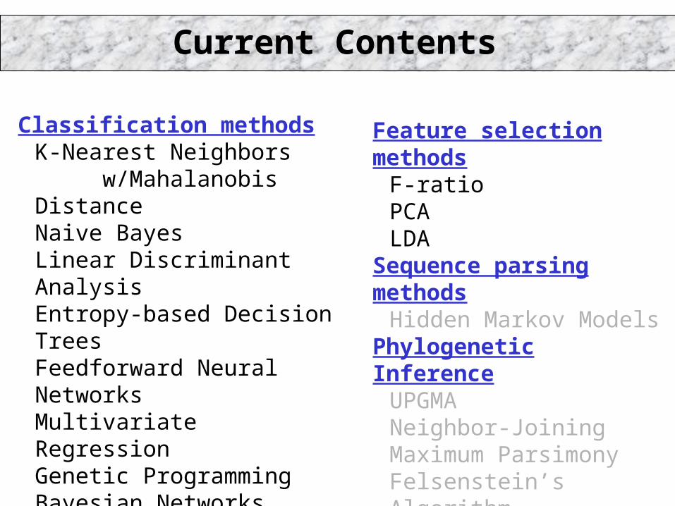
Classification methodsK-Nearest Neighbors

w/Mahalanobis DistanceNaive BayesLinear Discriminant AnalysisEntropy-based Decision TreesFeedforward Neural NetworksMultivariate RegressionGenetic ProgrammingBayesian NetworksLogistic Regression Simulated Annealing

Feature selection methodsF-ratioPCALDA

Sequence parsing methodsHidden Markov Models

Phylogenetic InferenceUPGMANeighbor-JoiningMaximum ParsimonyFelsenstein’s Algorithm

(grey = coming soon)

Current Contents

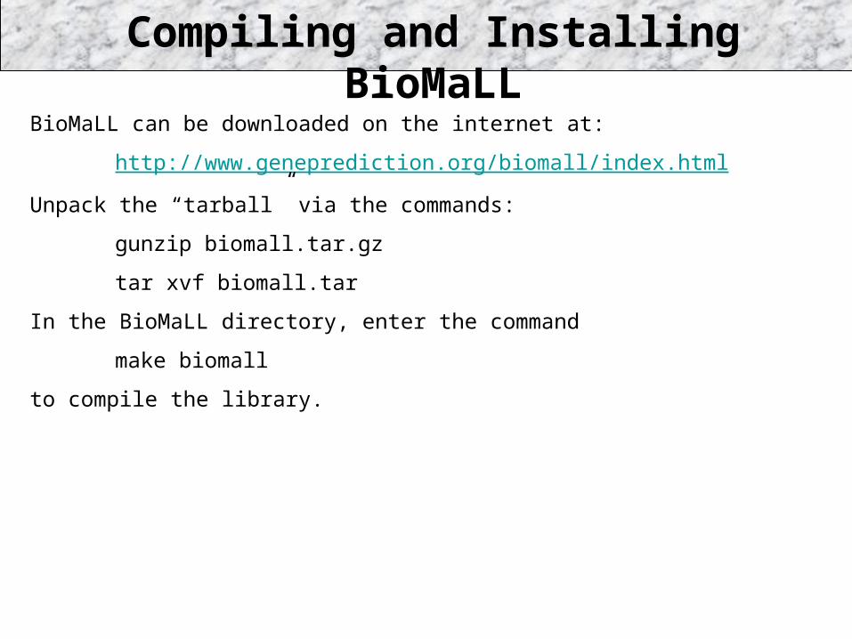
Compiling and Installing BioMaLL

BioMaLL can be downloaded on the internet at:

http://www.geneprediction.org/biomall/index.html

Unpack the “tarball” via the commands:

gunzip biomall.tar.gz

tar xvf biomall.tar

In the BioMaLL directory, enter the command

make biomall

to compile the library.

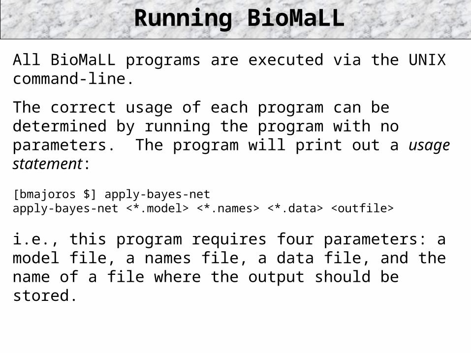
Running BioMaLL

All BioMaLL programs are executed via the UNIX command-line.

The correct usage of each program can be determined by running the program with no parameters. The program will print out a usage statement:

[bmajoros $] apply-bayes-netapply-bayes-net <*.model> <*.names> <*.data> <outfile>

i.e., this program requires four parameters: a model file, a names file, a data file, and the name of a file where the output should be stored.

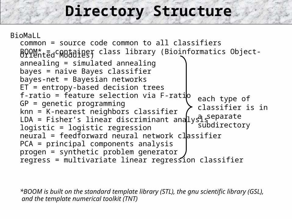
Directory Structure

BioMaLLcommon = source code common to all classifiersBOOM* = container class library (Bioinformatics Object-Oriented Modules)annealing = simulated annealingbayes = naive Bayes classifierbayes-net = Bayesian networksET = entropy-based decision treesf-ratio = feature selection via F-ratioGP = genetic programmingknn = K-nearest neighbors classifierLDA = Fisher’s linear discriminant analysislogistic = logistic regressionneural = feedforward neural network classifierPCA = principal components analysisprogen = synthetic problem generatorregress = multivariate linear regression classifier

*BOOM is built on the standard template library (STL), the gnu scientific library (GSL), and the template numerical toolkit (TNT)

each type of classifier is in a separate subdirectory

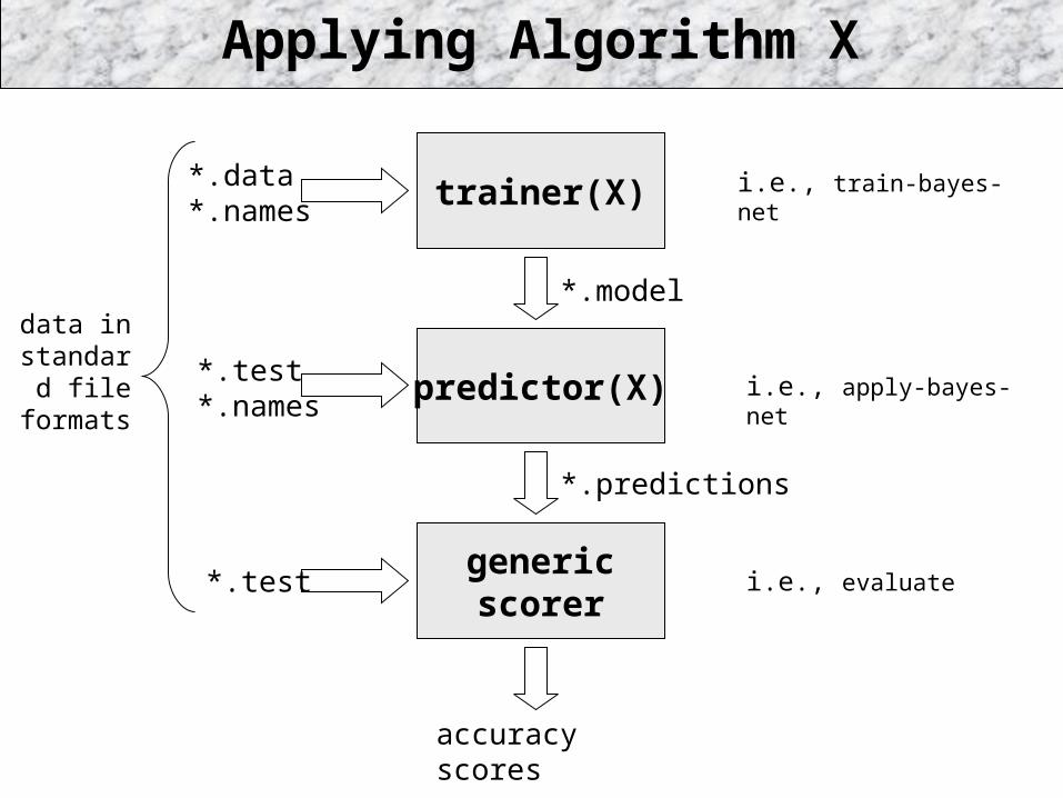
*.data *.names trainer(X)

predictor(X)

genericscorer

Applying Algorithm X

*.test *.names

*.test

*.model

*.predictions

accuracy scores

data in standard

file formats

i.e., train-bayes-net

i.e., apply-bayes-net

i.e., evaluate

File Formats

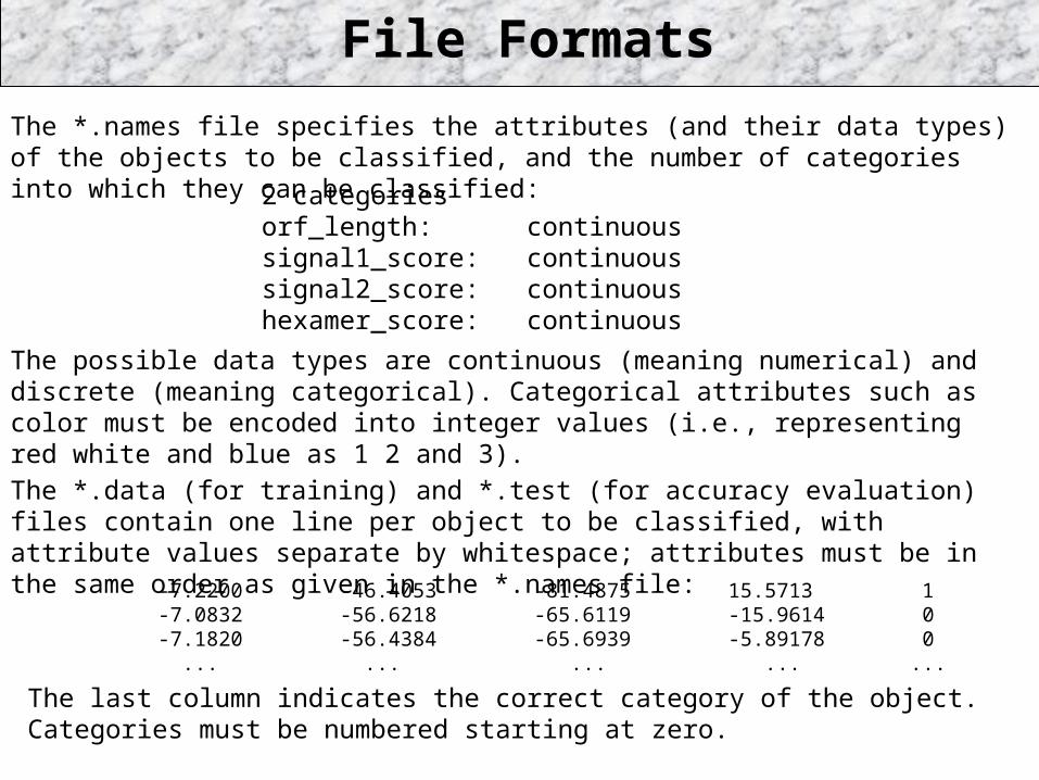
The *.names file specifies the attributes (and their data types) of the objects to be classified, and the number of categories into which they can be classified:

The *.data (for training) and *.test (for accuracy evaluation) files contain one line per object to be classified, with attribute values separate by whitespace; attributes must be in the same order as given in the *.names file:

2 categoriesorf_length: continuoussignal1_score: continuoussignal2_score: continuoushexamer_score: continuous

The possible data types are continuous (meaning numerical) and discrete (meaning categorical). Categorical attributes such as color must be encoded into integer values (i.e., representing red white and blue as 1 2 and 3).

-7.2200 -46.4053 -81.4875 15.5713 1-7.0832 -56.6218 -65.6119 -15.9614 0-7.1820 -56.4384 -65.6939 -5.89178 0 ... ... ... ... ...

The last column indicates the correct category of the object. Categories must be numbered starting at zero.

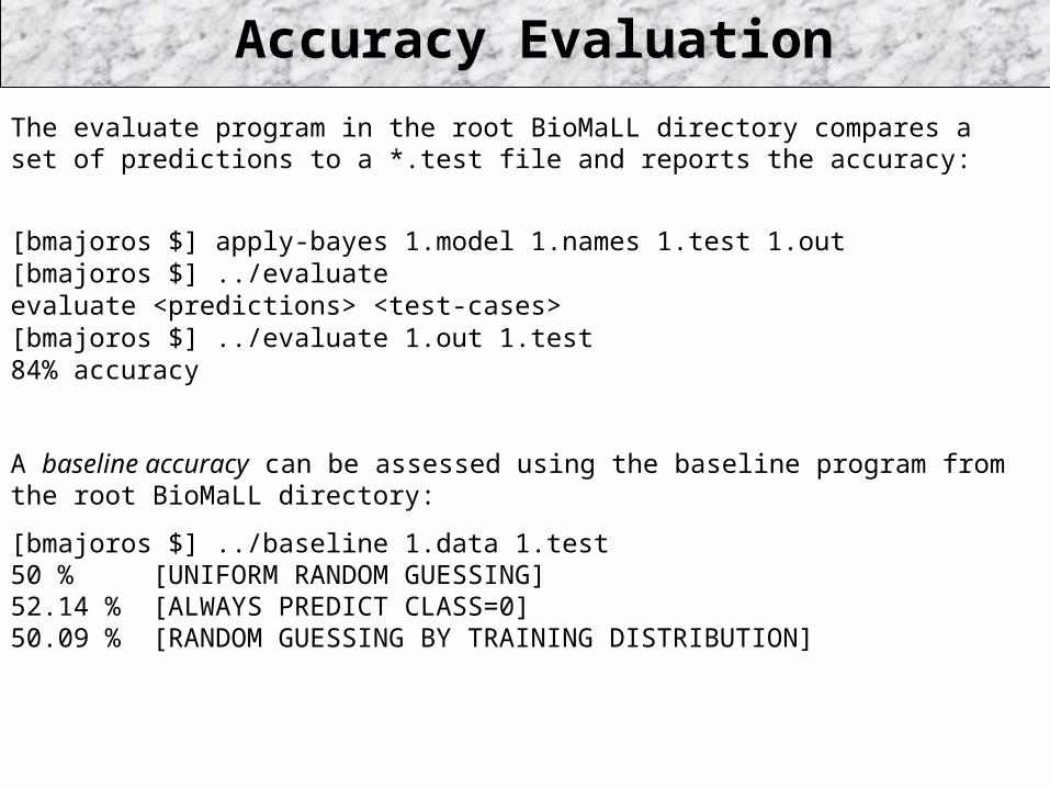
Accuracy Evaluation

The evaluate program in the root BioMaLL directory compares a set of predictions to a *.test file and reports the accuracy:

[bmajoros $] apply-bayes 1.model 1.names 1.test 1.out[bmajoros $] ../evaluateevaluate <predictions> <test-cases>[bmajoros $] ../evaluate 1.out 1.test84% accuracy

A baseline accuracy can be assessed using the baseline program from the root BioMaLL directory:

[bmajoros $] ../baseline 1.data 1.test50 % [UNIFORM RANDOM GUESSING]52.14 % [ALWAYS PREDICT CLASS=0]50.09 % [RANDOM GUESSING BY TRAINING DISTRIBUTION]

Part II

Algorithm Descriptions and Examples

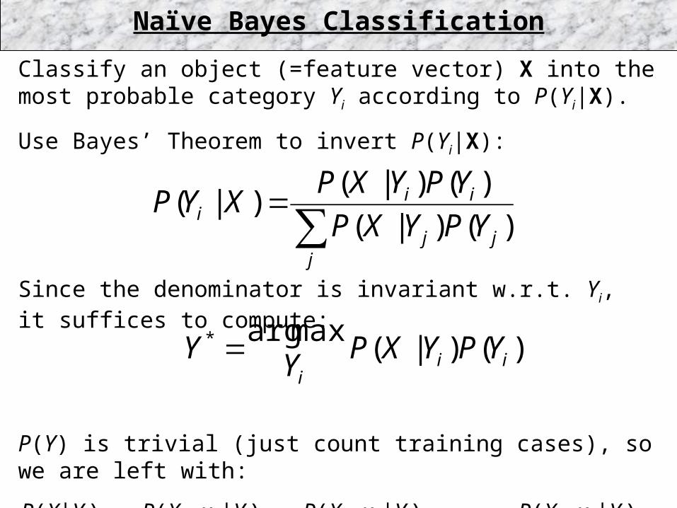
Since the denominator is invariant w.r.t. Yi, it suffices to compute:

P(Y) is trivial (just count training cases), so we are left with:

P(X|Yi) ≈ P(X1=x1|Yi) · P(X2=x2|Yi) · … · P(Xn=xn|Yi),

assuming conditional independence (the “naive Bayes” assumption).

Classify an object (=feature vector) X into the most probable category Yi according to P(Yi|X).

Use Bayes’ Theorem to invert P(Yi|X):

Naïve Bayes Classification

∑=

jjj

iii YPYXP

YPYXPXYP

)()|(

)()|()|(

)()|(maxarg*

iii

YPYXPY

Y =

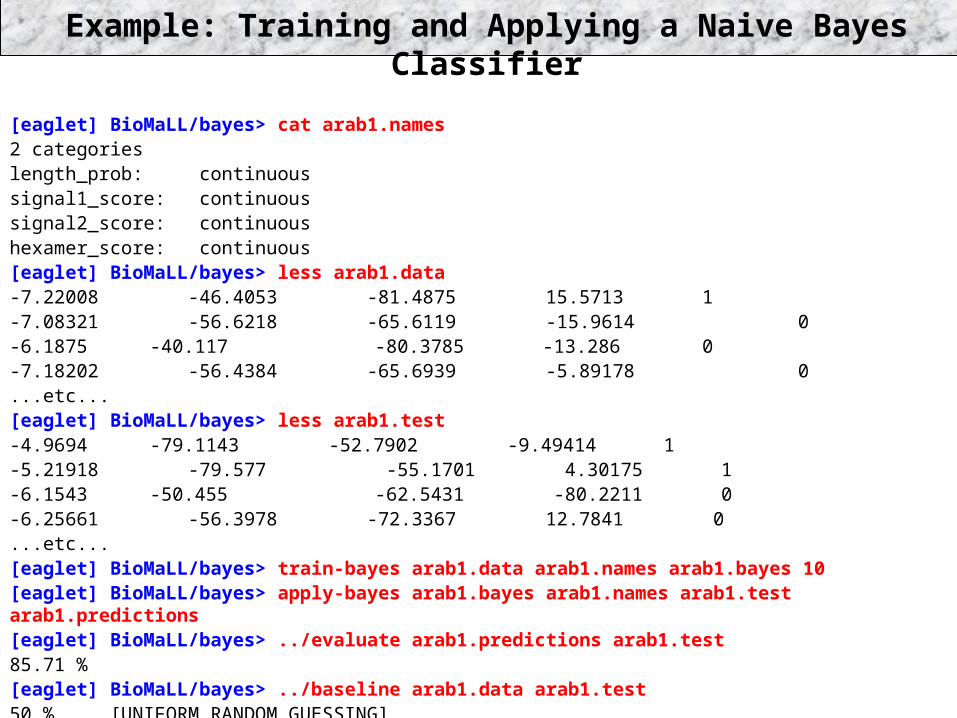
Example: Training and Applying a Naive Bayes Classifier

[eaglet] BioMaLL/bayes> cat arab1.names2 categorieslength_prob: continuoussignal1_score: continuoussignal2_score: continuoushexamer_score: continuous[eaglet] BioMaLL/bayes> less arab1.data-7.22008 -46.4053 -81.4875 15.5713 1-7.08321 -56.6218 -65.6119 -15.9614 0-6.1875 -40.117 -80.3785 -13.286 0-7.18202 -56.4384 -65.6939 -5.89178 0...etc...[eaglet] BioMaLL/bayes> less arab1.test-4.9694 -79.1143 -52.7902 -9.49414 1-5.21918 -79.577 -55.1701 4.30175 1-6.1543 -50.455 -62.5431 -80.2211 0-6.25661 -56.3978 -72.3367 12.7841 0...etc...[eaglet] BioMaLL/bayes> train-bayes arab1.data arab1.names arab1.bayes 10[eaglet] BioMaLL/bayes> apply-bayes arab1.bayes arab1.names arab1.test arab1.predictions[eaglet] BioMaLL/bayes> ../evaluate arab1.predictions arab1.test85.71 %[eaglet] BioMaLL/bayes> ../baseline arab1.data arab1.test50 % [UNIFORM RANDOM GUESSING]47.85 % [ALWAYS PREDICT CLASS=1]49.98 % [RANDOM GUESSING BY TRAINING DISTRIBUTION]

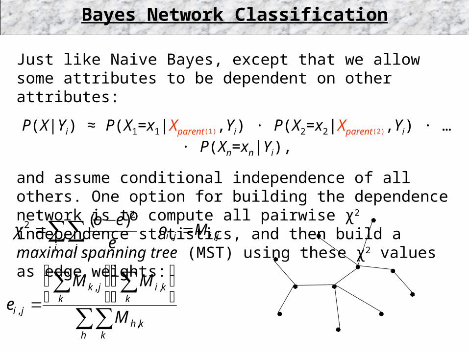
Just like Naive Bayes, except that we allow some attributes to be dependent on other attributes:

P(X|Yi) ≈ P(X1=x1|Xparent(1),Yi) · P(X2=x2|Xparent(2),Yi) · … · P(Xn=xn|Yi),

and assume conditional independence of all others. One option for building the dependence network is to compute all pairwise χ2 independence statistics, and then build a maximal spanning tree (MST) using these χ2 values as edge weights:

Bayes Network Classification

∑∑ −=

i j e

eo 22 )(

χ jiji Mo ,, =

∑∑∑∑ ⎟

⎠

⎞⎜⎝

⎛⎟⎠

⎞⎜⎝

⎛

=

h kkh

kki

kjk

ji M

MM

e,

,,

,

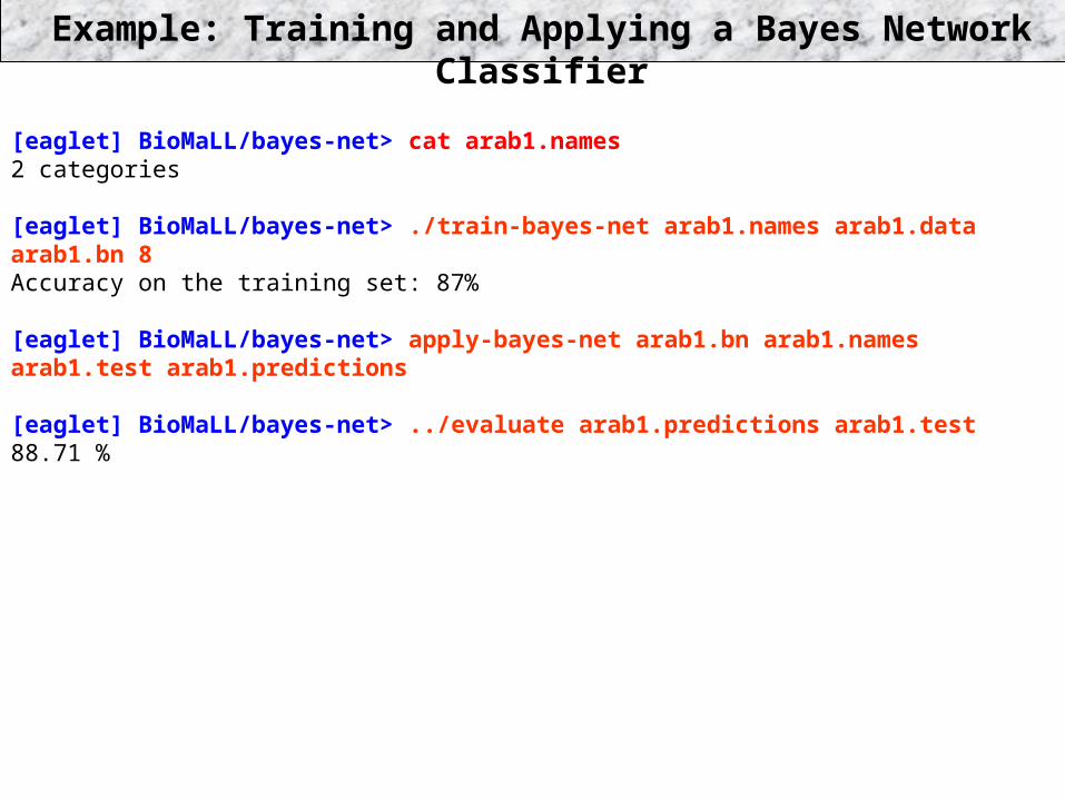
Example: Training and Applying a Bayes Network Classifier

[eaglet] BioMaLL/bayes-net> cat arab1.names2 categories

[eaglet] BioMaLL/bayes-net> ./train-bayes-net arab1.names arab1.data arab1.bn 8 Accuracy on the training set: 87%

[eaglet] BioMaLL/bayes-net> apply-bayes-net arab1.bn arab1.names arab1.test arab1.predictions

[eaglet] BioMaLL/bayes-net> ../evaluate arab1.predictions arab1.test88.71 %

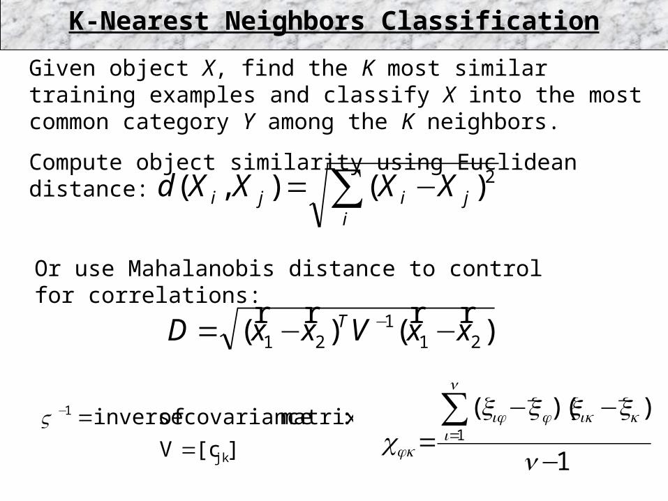
Given object X, find the K most similar training examples and classify X into the most common category Y among the K neighbors.

Compute object similarity using Euclidean distance:

∑ −=i

jiji XXXXd 2)(),(

Or use Mahalanobis distance to control for correlations:

K-Nearest Neighbors Classification

)()( 211

21 xxVxxD T rrrr −−= −

][cV

:matrix covariance of inverse

jk

1

==−V

1

))((1

−

−−=∑=

n

xxxxc

n

ikikjij

jk

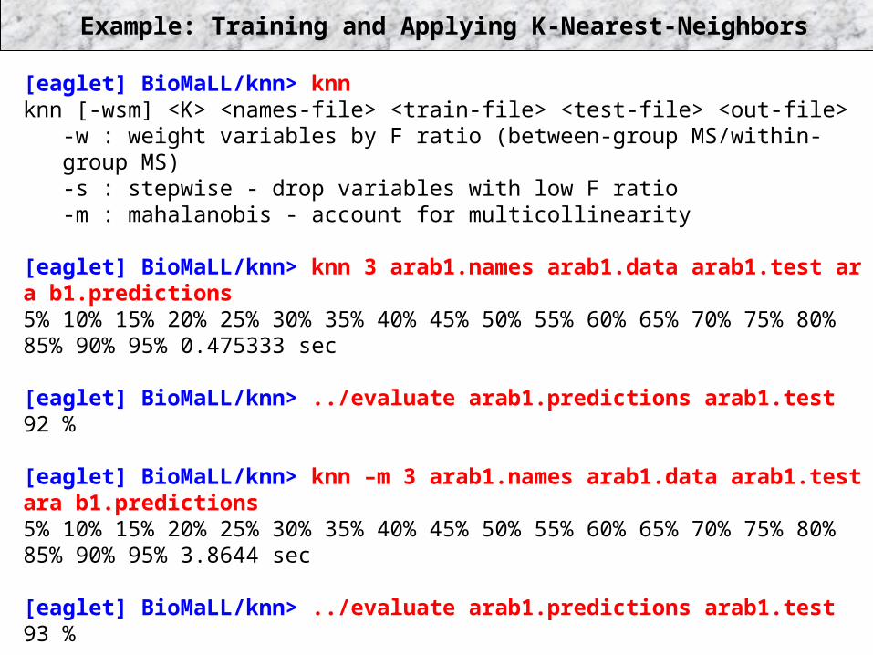
Example: Training and Applying K-Nearest-Neighbors

[eaglet] BioMaLL/knn> knnknn [-wsm] <K> <names-file> <train-file> <test-file> <out-file> -w : weight variables by F ratio (between-group MS/within- group MS) -s : stepwise - drop variables with low F ratio -m : mahalanobis - account for multicollinearity

[eaglet] BioMaLL/knn> knn 3 arab1.names arab1.data arab1.test ar a b1.predictions5% 10% 15% 20% 25% 30% 35% 40% 45% 50% 55% 60% 65% 70% 75% 80% 85% 90% 95% 0.475333 sec

[eaglet] BioMaLL/knn> ../evaluate arab1.predictions arab1.test92 %

[eaglet] BioMaLL/knn> knn –m 3 arab1.names arab1.data arab1.test ara b1.predictions5% 10% 15% 20% 25% 30% 35% 40% 45% 50% 55% 60% 65% 70% 75% 80% 85% 90% 95% 3.8644 sec

[eaglet] BioMaLL/knn> ../evaluate arab1.predictions arab1.test93 %

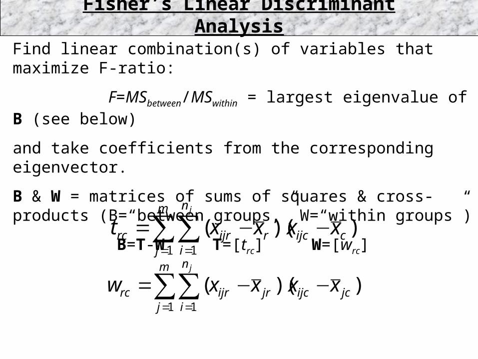
Find linear combination(s) of variables that maximize F-ratio:

F=MSbetween/MSwithin = largest eigenvalue of B (see below)

and take coefficients from the corresponding eigenvector.

B & W = matrices of sums of squares & cross-products (B=“between groups,” W=“within groups”)

B=T-W T=[trc] W=[wrc]

Apply significant eigenvectors as linear combinations, collect into a vector, and use nearest-centroid to classify test case.

Fisher’s Linear Discriminant Analysis

∑∑= =

−−=m

j

n

icijcrijrrc

j

xxxxt1 1

))((

∑∑= =

−−=m

j

n

ijcijcjrijrrc

j

xxxxw1 1

))((

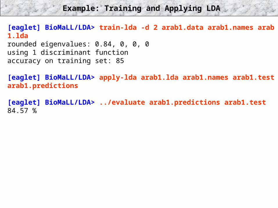
Example: Training and Applying LDA

[eaglet] BioMaLL/LDA> train-lda -d 2 arab1.data arab1.names arab 1.ldarounded eigenvalues: 0.84, 0, 0, 0using 1 discriminant functionaccuracy on training set: 85

[eaglet] BioMaLL/LDA> apply-lda arab1.lda arab1.names arab1.test arab1.predictions

[eaglet] BioMaLL/LDA> ../evaluate arab1.predictions arab1.test84.57 %

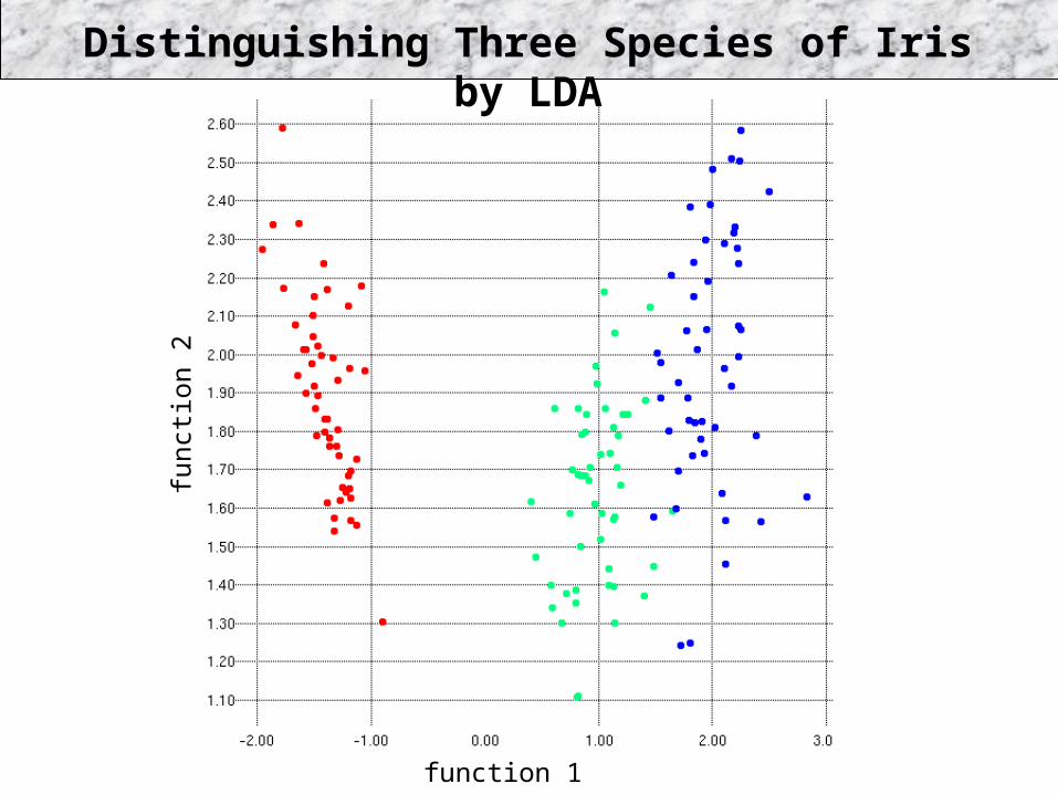
Distinguishing Three Species of Iris by LDA

function 1

func

tion

2

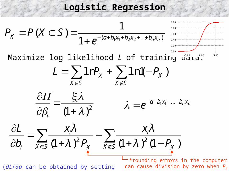
Logistic Regression

)...( 22111

1)(

nn xbxbxbaX eSXPP ++++−+

=∈=

∑∑∉∈

−+=SX

XSX

X PPL )1ln(ln

Maximize log-likelihood L of training data:

2)1( λλ

+=

∂∂ i

i

xbP

nn xbxbae −−−−= ...11λ

∑∑∉∈ −+

−+

=∂∂

SX X

i

SX X

i

i P

x

P

x

b

L

)1()1()1( 22 λ

λ

λ

λ

(∂L/∂a can be obtained by setting xi=1)*rounding errors in the computer can cause division by zero when PX approaches 0 or 1

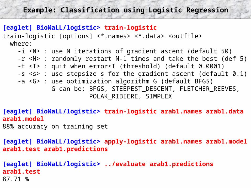
Example: Classification using Logistic Regression

[eaglet] BioMaLL/logistic> train-logistictrain-logistic [options] <*.names> <*.data> <outfile> where: -i <N> : use N iterations of gradient ascent (default 50) -r <N> : randomly restart N-1 times and take the best (def 5) -t <T> : quit when error<T (threshold) (default 0.0001) -s <s> : use stepsize s for the gradient ascent (default 0.1) -a <G> : use optimization algorithm G (default BFGS) G can be: BFGS, STEEPEST_DESCENT, FLETCHER_REEVES, POLAK_RIBIERE, SIMPLEX

[eaglet] BioMaLL/logistic> train-logistic arab1.names arab1.data arab1.model88% accuracy on training set

[eaglet] BioMaLL/logistic> apply-logistic arab1.names arab1.model arab1.test arab1.predictions

[eaglet] BioMaLL/logistic> ../evaluate arab1.predictions arab1.test87.71 %

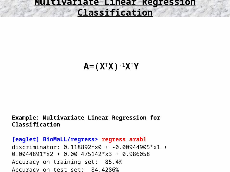
Multivariate Linear Regression Classification

A=(XTX)-1XTY

Example: Multivariate Linear Regression for Classification

[eaglet] BioMaLL/regress> regress arab1discriminator: 0.118892*x0 + -0.00944905*x1 + 0.0044891*x2 + 0.00 475142*x3 + 0.986058Accuracy on training set: 85.4%Accuracy on test set: 84.4286%

Feathered?

Volant?

Category=ratite Carnivorous?

Category=raptor

Endothermic?

Objects to be classified

Viviparous?

… ...

YES

YES

YES YES

YES

NO

NO

NO

NO

NO

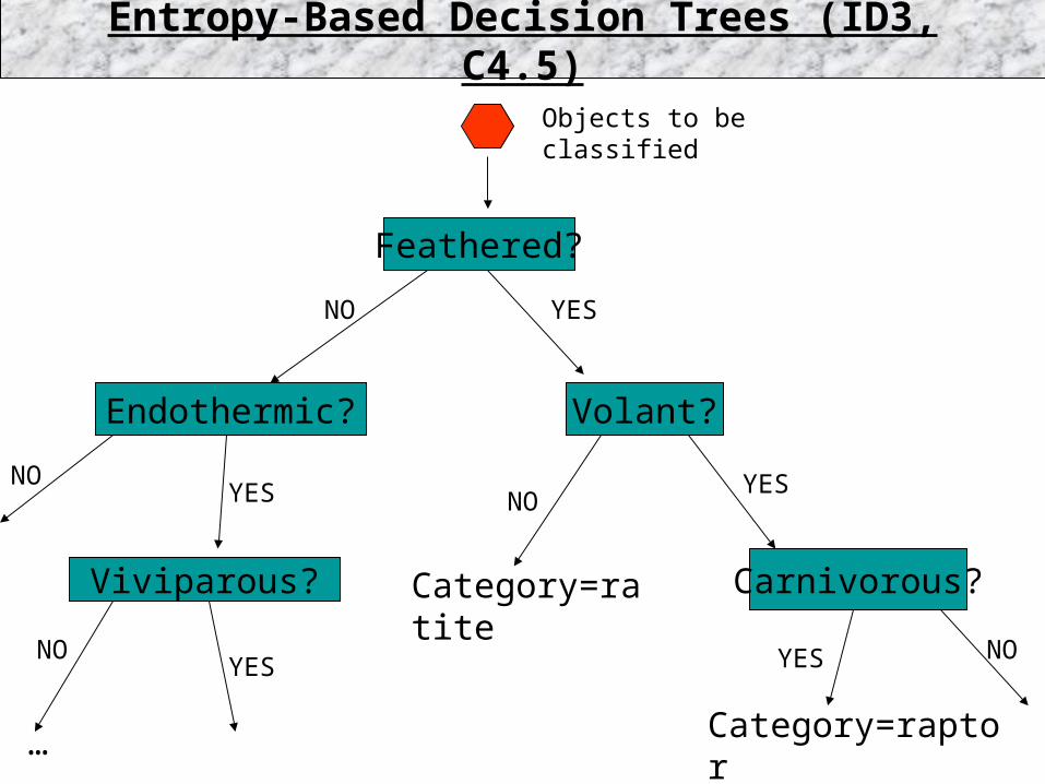
Entropy-Based Decision Trees (ID3, C4.5)

Predicate #k

truefalse

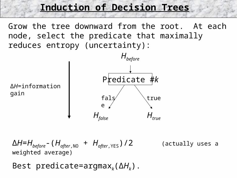
Grow the tree downward from the root. At each node, select the predicate that maximally reduces entropy (uncertainty):

Hbefore

Hfalse Htrue

ΔH=Hbefore-(Hafter,NO + Hafter,YES)/2 (actually uses a weighted average)

Best predicate=argmaxk(ΔHk).

Can also use gain ratio, but I found no difference in performance.

Induction of Decision Trees

ΔH=information gain

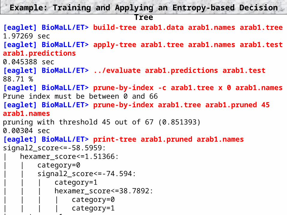
Example: Training and Applying an Entropy-based Decision Tree[eaglet] BioMaLL/ET> build-tree arab1.data arab1.names arab1.tree1.97269 sec[eaglet] BioMaLL/ET> apply-tree arab1.tree arab1.names arab1.test arab1.predictions0.045388 sec[eaglet] BioMaLL/ET> ../evaluate arab1.predictions arab1.test88.71 %[eaglet] BioMaLL/ET> prune-by-index -c arab1.tree x 0 arab1.namesPrune index must be between 0 and 66[eaglet] BioMaLL/ET> prune-by-index arab1.tree arab1.pruned 45 arab1.namespruning with threshold 45 out of 67 (0.851393)0.00304 sec[eaglet] BioMaLL/ET> print-tree arab1.pruned arab1.namessignal2_score<=-58.5959:| hexamer_score<=1.51366:| | category=0| | signal2_score<=-74.594:| | | category=1| | | hexamer_score<=38.7892:| | | | category=0| | | | category=1| category=1

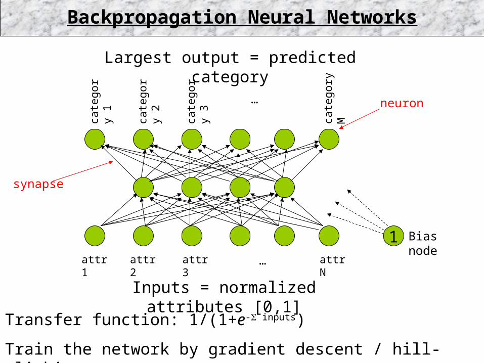
Transfer function: 1/(1+e- inputs)

Train the network by gradient descent / hill-climbing.

1 Bias node

attr 1 attr 2 attr 3 … attr N

Inputs = normalized attributes [0,1]

cate

gory

1

cate

gory

2

cate

gory

3

cate

gory

M

…

Largest output = predicted category

Backpropagation Neural Networks

neuron

synapse

jkkkkjk

k

k

k

kjk

ooootw

in

in

o

o

E

w

E)1()( −−−=

∂∂

∂∂

∂∂

=∂∂

jkjk w

Ew

∂∂

−=Δ η

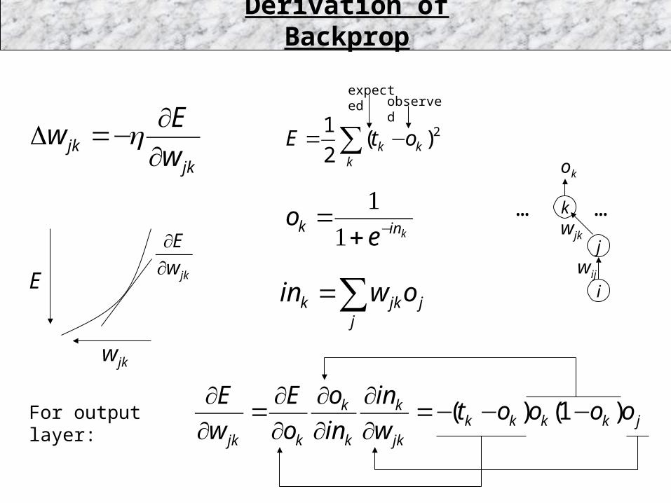
Derivation of Backprop

For output layer:

k

j

i

……kink e

o −+=

11

jj

jkk owin ∑=

wjk

∑ −=k

kk otE 2)(2

1

jkw

E

∂∂

E

wjk

wij

ok

expectedobserved

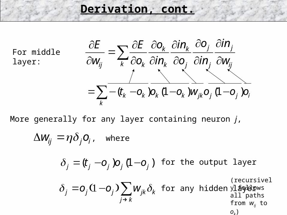
Derivation, cont.

ijij ow ηδ=Δ

More generally for any layer containing neuron j,

)1()( jjjjj ooot −−=δ

kkj

jkjjj woo δδ ∑→

−= )1( for any hidden layer

for the output layer

, where

∑ ∂∂

∂∂

∂∂

∂∂

∂∂

=∂∂

k ij

j

j

j

j

k

k

k

kij w

in

in

o

o

in

in

o

o

E

w

E

∑ −−−−=k

ijjjkkkkk ooowooot )1()1()(

For middle layer:

(recursively follows all paths from wij to ok)

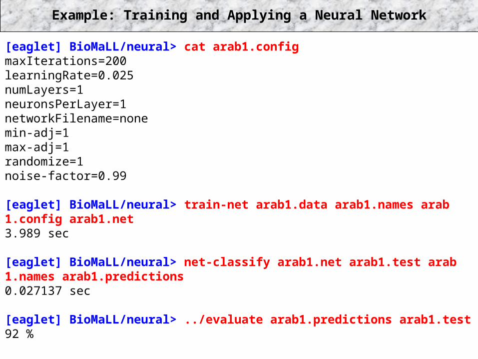
Example: Training and Applying a Neural Network

[eaglet] BioMaLL/neural> cat arab1.configmaxIterations=200learningRate=0.025numLayers=1neuronsPerLayer=1networkFilename=nonemin-adj=1max-adj=1randomize=1noise-factor=0.99

[eaglet] BioMaLL/neural> train-net arab1.data arab1.names arab 1.config arab1.net3.989 sec

[eaglet] BioMaLL/neural> net-classify arab1.net arab1.test arab 1.names arab1.predictions0.027137 sec

[eaglet] BioMaLL/neural> ../evaluate arab1.predictions arab1.test92 %

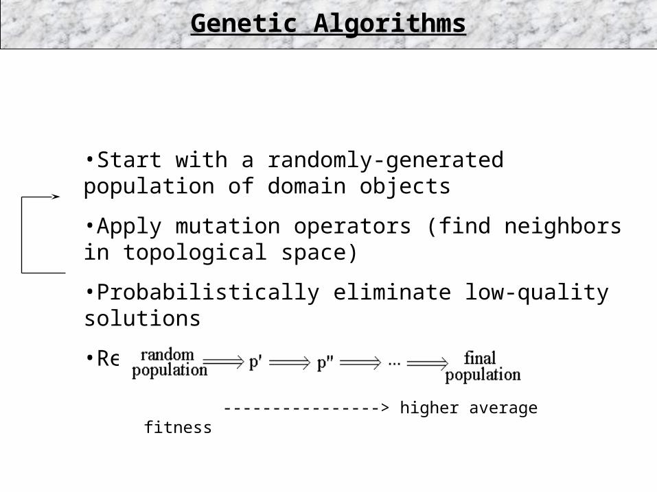
•Start with a randomly-generated population of domain objects

•Apply mutation operators (find neighbors in topological space)

•Probabilistically eliminate low-quality solutions

•Repeat until convergence

----------------> higher average fitness

Genetic Algorithms

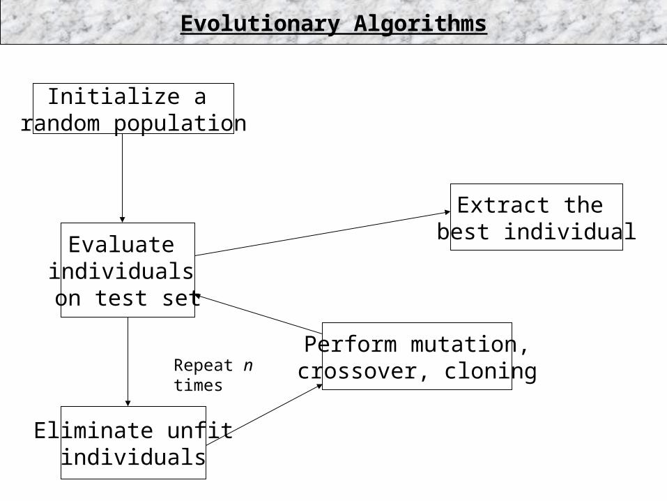
Initialize a random population

Evaluate individuals on test set

Eliminate unfitindividuals

Perform mutation,crossover, cloning

Evolutionary Algorithms

Extract the best individual

Repeat n times

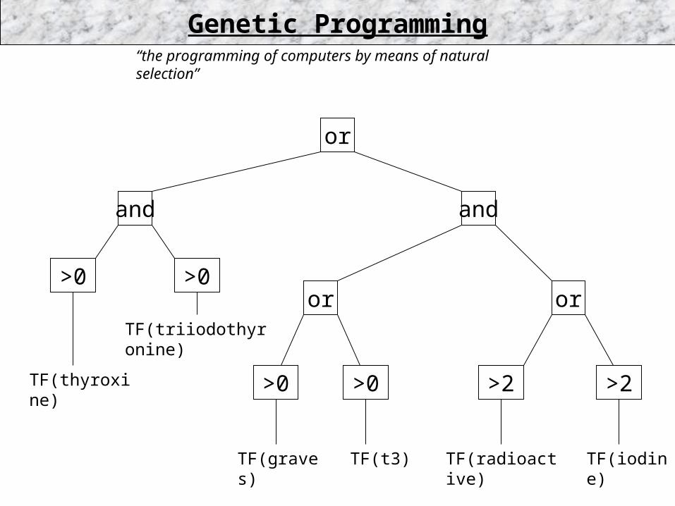
“the programming of computers by means of natural selection”

or

andand

or or

TF(iodine)

TF(triiodothyronine)

TF(radioactive)

TF(thyroxine)

TF(graves) TF(t3)

>2>0 >2>0

>0>0

Genetic Programming

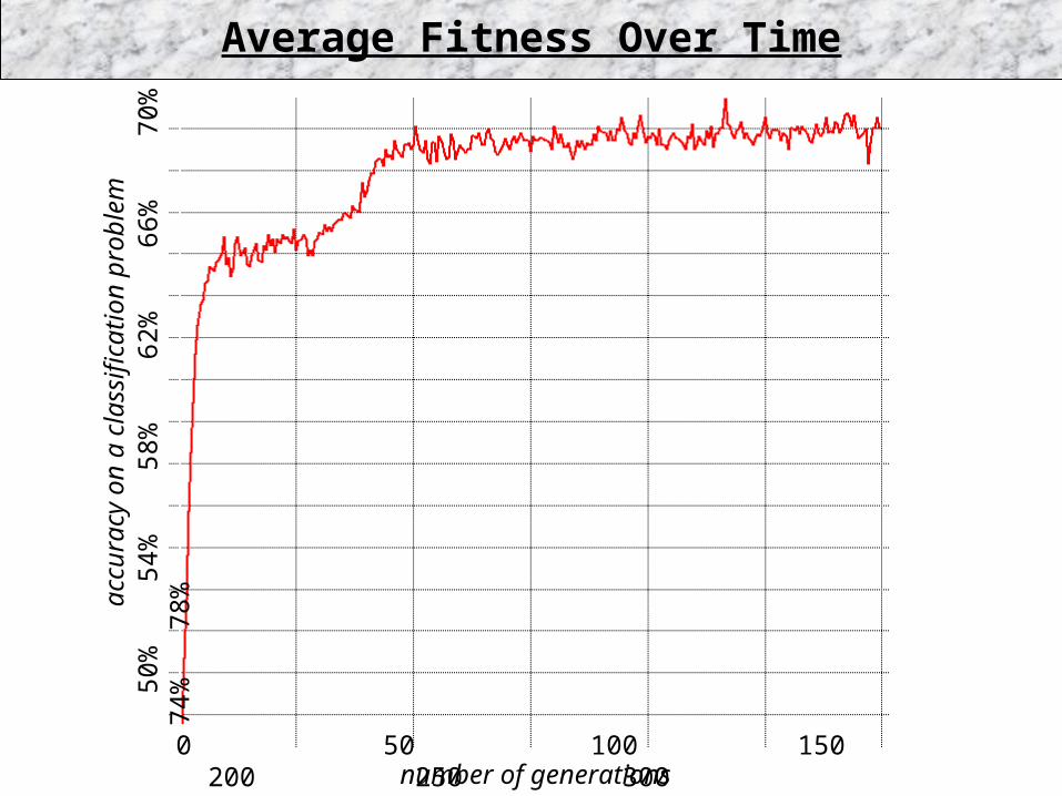
Average Fitness Over Time

0 50 100 150 200 250 300number of generations

accu

racy

on

a cl

assi

fica

tion

pro

blem

50%

54%

58%

62%

66%

70%

74%

7

8%

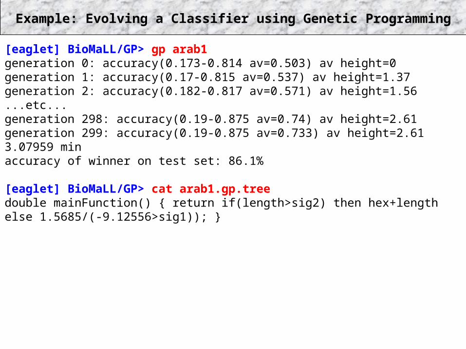
Example: Evolving a Classifier using Genetic Programming

[eaglet] BioMaLL/GP> gp arab1generation 0: accuracy(0.173-0.814 av=0.503) av height=0generation 1: accuracy(0.17-0.815 av=0.537) av height=1.37generation 2: accuracy(0.182-0.817 av=0.571) av height=1.56...etc...generation 298: accuracy(0.19-0.875 av=0.74) av height=2.61generation 299: accuracy(0.19-0.875 av=0.733) av height=2.613.07959 minaccuracy of winner on test set: 86.1%

[eaglet] BioMaLL/GP> cat arab1.gp.treedouble mainFunction() { return if(length>sig2) then hex+length else 1.5685/(-9.12556>sig1)); }

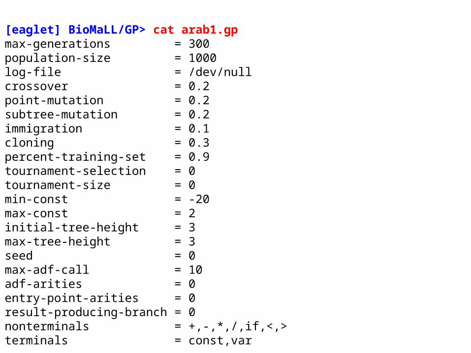
[eaglet] BioMaLL/GP> cat arab1.gpmax-generations = 300population-size = 1000log-file = /dev/nullcrossover = 0.2point-mutation = 0.2subtree-mutation = 0.2immigration = 0.1cloning = 0.3percent-training-set = 0.9tournament-selection = 0tournament-size = 0min-const = -20max-const = 2initial-tree-height = 3max-tree-height = 3seed = 0max-adf-call = 10adf-arities = 0entry-point-arities = 0result-producing-branch = 0nonterminals = +,-,*,/,if,<,>terminals = const,var

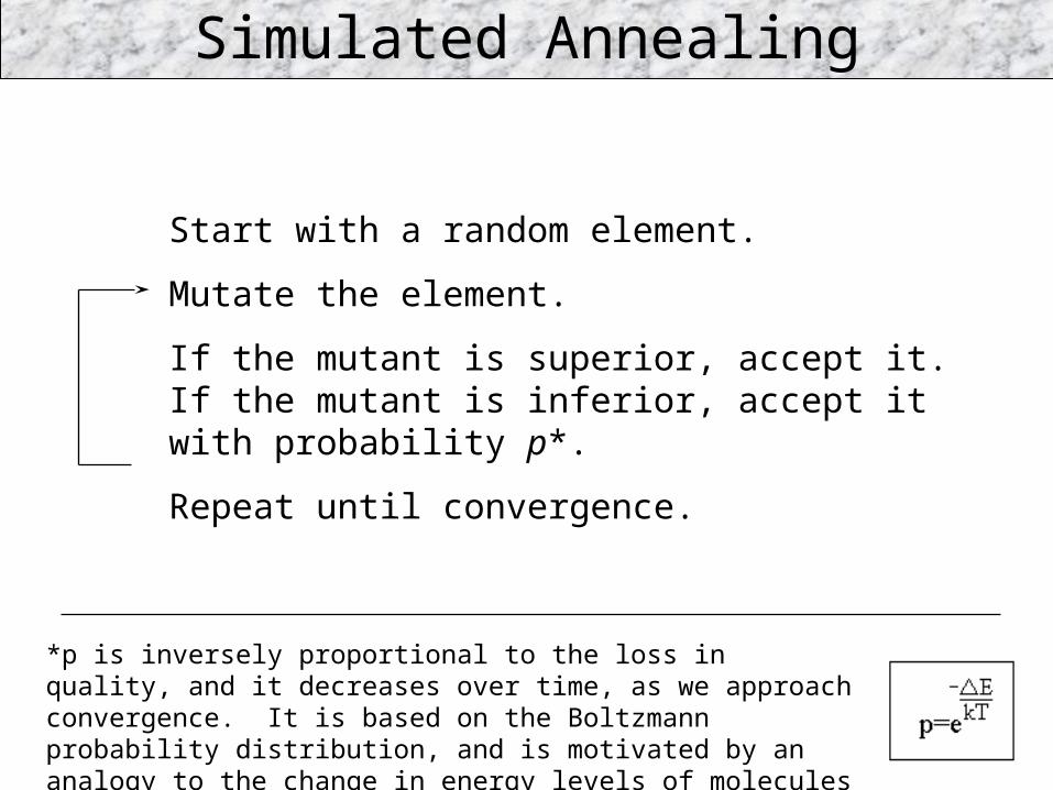
Simulated Annealing

Start with a random element.

Mutate the element.

If the mutant is superior, accept it. If the mutant is inferior, accept it with probability p*.

Repeat until convergence.

*p is inversely proportional to the loss in quality, and it decreases over time, as we approach convergence. It is based on the Boltzmann probability distribution, and is motivated by an analogy to the change in energy levels of molecules as the temperature is slowly decreased (i.e., time elapses).

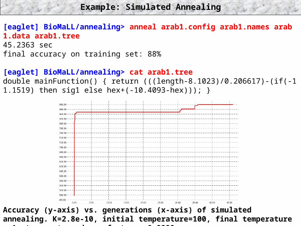
Example: Simulated Annealing

[eaglet] BioMaLL/annealing> anneal arab1.config arab1.names arab 1.data arab1.tree45.2363 secfinal accuracy on training set: 88%

[eaglet] BioMaLL/annealing> cat arab1.treedouble mainFunction() { return (((length-8.1023)/0.206617)-(if(-1 1.1519) then sig1 else hex+(-10.4093-hex))); }

Accuracy (y-axis) vs. generations (x-axis) of simulated annealing. K=2.8e-10, initial temperature=100, final temperature = 1, temperature decay factor = 0.9999.

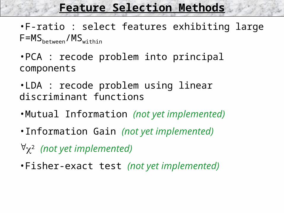
•F-ratio : select features exhibiting large F=MSbetween/MSwithin

•PCA : recode problem into principal components

•LDA : recode problem using linear discriminant functions

•Mutual Information (not yet implemented)

•Information Gain (not yet implemented)

2 (not yet implemented)

•Fisher-exact test (not yet implemented)

Feature Selection Methods

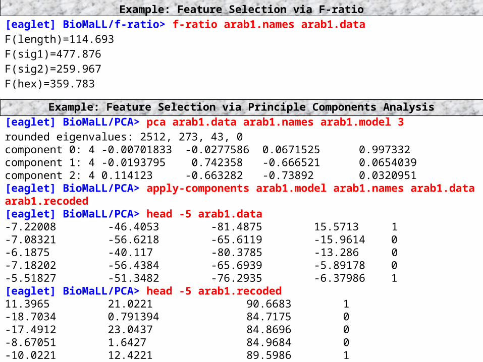
Example: Feature Selection via F-ratio[eaglet] BioMaLL/f-ratio> f-ratio arab1.names arab1.dataF(length)=114.693F(sig1)=477.876F(sig2)=259.967F(hex)=359.783

Example: Feature Selection via Principle Components Analysis[eaglet] BioMaLL/PCA> pca arab1.data arab1.names arab1.model 3rounded eigenvalues: 2512, 273, 43, 0component 0: 4 -0.00701833 -0.0277586 0.0671525 0.997332component 1: 4 -0.0193795 0.742358 -0.666521 0.0654039component 2: 4 0.114123 -0.663282 -0.73892 0.0320951[eaglet] BioMaLL/PCA> apply-components arab1.model arab1.names arab1.data arab1.recoded[eaglet] BioMaLL/PCA> head -5 arab1.data-7.22008 -46.4053 -81.4875 15.5713 1-7.08321 -56.6218 -65.6119 -15.9614 0-6.1875 -40.117 -80.3785 -13.286 0-7.18202 -56.4384 -65.6939 -5.89178 0-5.51827 -51.3482 -76.2935 -6.37986 1[eaglet] BioMaLL/PCA> head -5 arab1.recoded11.3965 21.0221 90.6683 1-18.7034 0.791394 84.7175 0-17.4912 23.0437 84.8696 0-8.67051 1.6427 84.9684 0-10.0221 12.4221 89.5986 1

Part III

Sample Data Sets

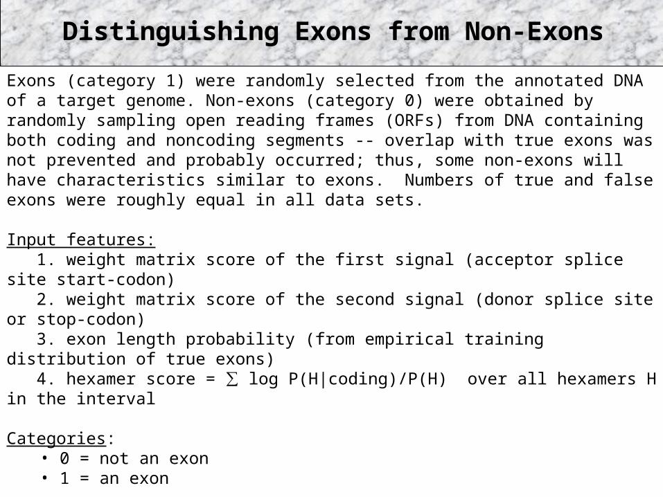
Distinguishing Exons from Non-Exons

Exons (category 1) were randomly selected from the annotated DNA of a target genome. Non-exons (category 0) were obtained by randomly sampling open reading frames (ORFs) from DNA containing both coding and noncoding segments -- overlap with true exons was not prevented and probably occurred; thus, some non-exons will have characteristics similar to exons. Numbers of true and false exons were roughly equal in all data sets.

Input features: 1. weight matrix score of the first signal (acceptor splice site start-codon) 2. weight matrix score of the second signal (donor splice site or stop-codon) 3. exon length probability (from empirical training distribution of true exons) 4. hexamer score = ∑ log P(H|coding)/P(H) over all hexamers H in the interval

Categories:• 0 = not an exon• 1 = an exon

Data sets:arab1 = arabidopsis thalianahuman1 = homo sapiensaspergillus1 = aspergillus fumigatus