Machine Learning Algorithms for Graph-Based ...research.cgu.edu/mathematics-clinic/wp-content/uploads/sites/21/... · Machine Learning Algorithms for Graph-Based ... 2.3 Support Vector

Final Report for

Los Alamos National Laboratory

Machine Learning Algorithms for Graph-BasedRepresentations of Fracture Networks

Fall 2016 – Spring 2017

Team Members

Adrian CantuZhengyang (Michael) GuoPriscilla KellySean MatzManuel Valera (Project Manager)

Advisor

Allon Percus

Liaisons

Jeffrey HymanGowri SrinivasanHari Viswanathan

Abstract

Microstructural information, such as fracture size, geometry, aperture, and ma-terial properties, plays a key role in modeling the dominant physics for flowpropagation through fractured rock. Discrete fracture network (DFN) compu-tational suites, such as DFNWORKS, have recently been developed to simulateflow and transport in such media. These methods allow for particle tracking, re-vealing a small backbone of fractures through which most transport occurs, andtherefore providing a significant reduction in the effective size of the fracturenetwork. However, the simulations needed for particle tracking are computa-tionally intensive, and may not be scalable to large systems.

In this Mathematics Clinic project, conducted at Claremont Graduate Uni-versity under the sponsorship of Los Alamos National Laboratory, we introducea machine learning approach to characterizing transport in DFNs. We considera graph representation where nodes signify fractures and edges denote their in-tersections. Using supervised learning techniques that train on particle-trackingbackbone paths found by DFNWORKS, we predict whether or not fractures con-duct significant flow, based primarily on node centrality features in the graph.Our methods run in negligible time compared to particle-tracking simulations.We find that our predicted backbone can reduce the network to approximately20% of its original size, while still generating breakthrough curves in close agree-ment with those of the full network. Finally, we present a modeling frameworkfor the dynamic problem of fracture propagation, ultimately intended to providerapid predictions of when and where material failure occurs.

Contents

Abstract 3

1 Introduction 71.1 Sponsor . . . . . . . . . . . . . . . . . . . . . . . . . . . . . . . . . . . . 71.2 Background . . . . . . . . . . . . . . . . . . . . . . . . . . . . . . . . . 71.3 Project Goals . . . . . . . . . . . . . . . . . . . . . . . . . . . . . . . . . 9

2 Classification Methods 152.1 Node Features . . . . . . . . . . . . . . . . . . . . . . . . . . . . . . . . 162.2 Random Forest . . . . . . . . . . . . . . . . . . . . . . . . . . . . . . . 222.3 Support Vector Machines . . . . . . . . . . . . . . . . . . . . . . . . . 242.4 Two-Stage Method . . . . . . . . . . . . . . . . . . . . . . . . . . . . . 272.5 Dynamic Graph . . . . . . . . . . . . . . . . . . . . . . . . . . . . . . . 28

3 Results 313.1 Performance Measures . . . . . . . . . . . . . . . . . . . . . . . . . . . 313.2 Random Forest . . . . . . . . . . . . . . . . . . . . . . . . . . . . . . . 323.3 Support Vector Machine . . . . . . . . . . . . . . . . . . . . . . . . . . 353.4 Validation . . . . . . . . . . . . . . . . . . . . . . . . . . . . . . . . . . 373.5 Two-Stage Method . . . . . . . . . . . . . . . . . . . . . . . . . . . . . 403.6 Dynamic Graph . . . . . . . . . . . . . . . . . . . . . . . . . . . . . . . 40

4 Conclusions 43

A Code Description 45A.1 Dependencies . . . . . . . . . . . . . . . . . . . . . . . . . . . . . . . . 45A.2 Quick start . . . . . . . . . . . . . . . . . . . . . . . . . . . . . . . . . . 45A.3 Files . . . . . . . . . . . . . . . . . . . . . . . . . . . . . . . . . . . . . . 46A.4 Folders . . . . . . . . . . . . . . . . . . . . . . . . . . . . . . . . . . . . 47

Bibliography 49

Chapter 1

Introduction

1.1 Sponsor

Our CGU Math Clinic team has been working under the sponsorship of LosAlamos National Laboratory (LANL), a United States Department of Energy na-tional laboratory located in Los Alamos, New Mexico. LANL was established in1943 to develop nuclear weapons during World War II. A current effort at LANLinvolves developing a method of modeling fractures which can exist in shale gasreserves and after nuclear underground explosions. In order to make the pro-cess more computationally efficient, they aim to develop machine learning al-gorithms to characterize primary flow subnetworks within fractured subsurfacematerials, and to model the development and propagation of fractures underload.

1.2 Background

Discrete fracture networks (DFN) have been a topic of interest since 1990 whenresearchers began applying network theory to fracture networks [1]. High valueapplications, such as water quality monitoring [2], accessing natural gas [3, 4],and the monitoring of gas emissions [5] have motivated the development ofhigh-fidelity models which could be used to predict flow.

Large rock structures contain connected networks of fractures that conductfluid. The DFN models a fracture network as a random set of intersecting frac-ture planes, whose statistical properties match those of the original material.These statistical properties can include a multitude of hydrological and geomet-ric quantities associated with each plane. Computational suites such as DFN-WORKS [6], developed at LANL, use these properties to simulate flow and trans-

8 Introduction

port through the fracture. Such simulations allow more accurate prediction offluid mechanics than is typically possible using continuum models [7, 8]. Onthe other hand, a subsurface fracture network can typically contain millions offractures, with thousands of volume elements needed to describe each fracture.Resolving flow in such a structure is an enormous computational undertaking.

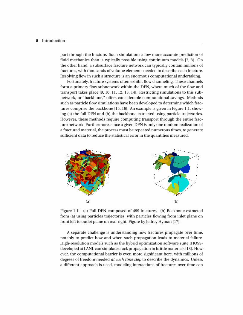
Fortunately, fracture systems often exhibit flow channeling. These channelsform a primary flow subnetwork within the DFN, where much of the flow andtransport takes place [9, 10, 11, 12, 13, 14]. Restricting simulations to this sub-network, or “backbone,” offers considerable computational savings. Methodssuch as particle flow simulations have been developed to determine which frac-tures comprise the backbone [15, 16]. An example is given in Figure 1.1, show-ing (a) the full DFN and (b) the backbone extracted using particle trajectories.However, these methods require computing transport through the entire frac-ture network. Furthermore, since a given DFN is only one random realization ofa fractured material, the process must be repeated numerous times, to generatesufficient data to reduce the statistical error in the quantities measured.

(a) (b)

Figure 1.1: (a) Full DFN composed of 499 fractures. (b) Backbone extractedfrom (a) using particles trajectories, with particles flowing from inlet plane onfront left to outlet plane on rear right. Figure by Jeffrey Hyman [17].

A separate challenge is understanding how fractures propagate over time,notably to predict how and when such propagation leads to material failure.High-resolution models such as the hybrid optimization software suite (HOSS)developed at LANL can simulate crack propagation in brittle materials [18]. How-ever, the computational barrier is even more significant here, with millions ofdegrees of freedom needed at each time step to describe the dynamics. Unlessa different approach is used, modeling interactions of fractures over time can

Project Goals 9

quickly become intractable.

1.3 Project Goals

It has been observed that flow through sparse fracture networks is governedmore by the network topology, namely which fractures connect to which others,than by the hydrological details of the fractures [19]. This raises the question ofwhether it is possible to identify the backbone of the network purely from topo-logical characteristics. Doing so would solve the computational bottleneck ofhaving to simulate flow and transport explicitly. The difficulty is determiningexactly how to combine topological properties for this purpose.

In recent years, there has been increased interest in the use of machine learn-ing in the geosciences. A range of different regression and classification methodshave been applied to a model of landslide susceptibility, demonstrating theirpredictive value [20]. Community detection methods have been used in frac-tured rock samples to identify regions expected to have high flow conductiv-ity [21]. Clustering analysis has been used in subsurface systems to constructmore accurate flow inversion algorithms [22]. The main goal of the 2016–17CGU Math Clinic project is to use machine learning techniques to reduce DFNsto subnetworks that carry most of the network’s flow. By treating topologicalproperties as features that describe fractures in the network, we develop fastclassification methods that learn to characterize the backbone in the featurespace.

Python code for all of our classification methods is available on our projectGitHub site. The code is organized into jupyter notebooks, which are describedin Appendix A.

1.3.1 Graph representation

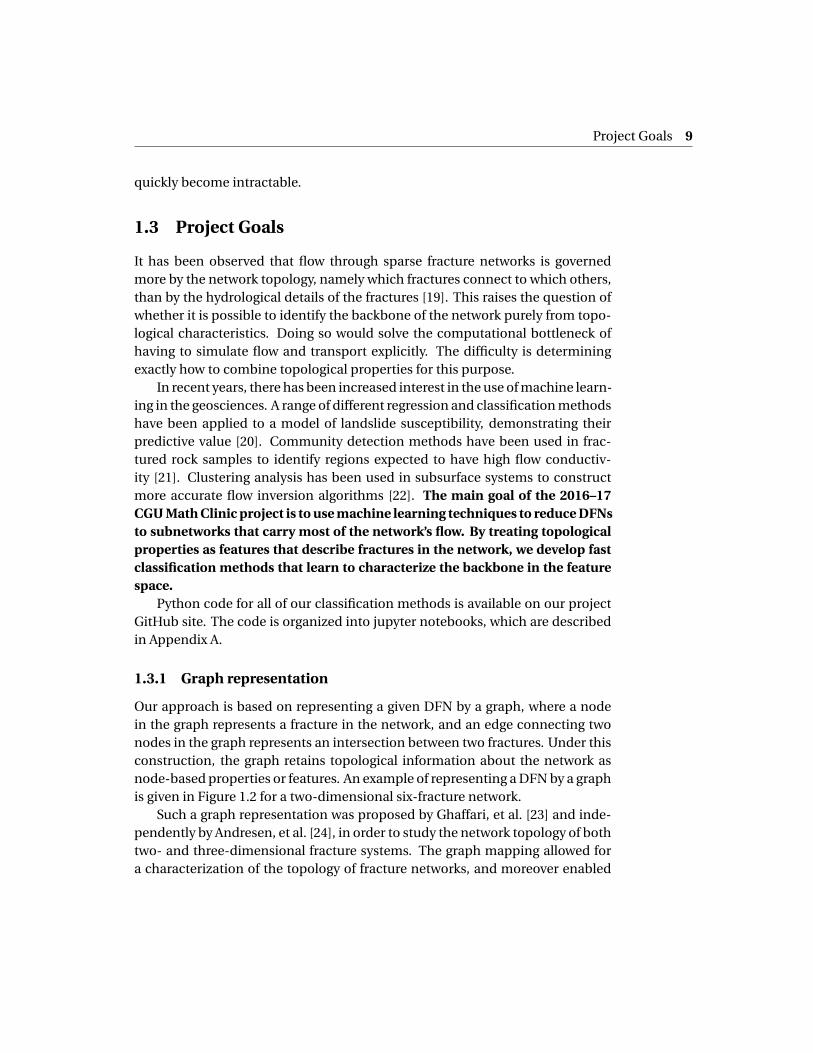
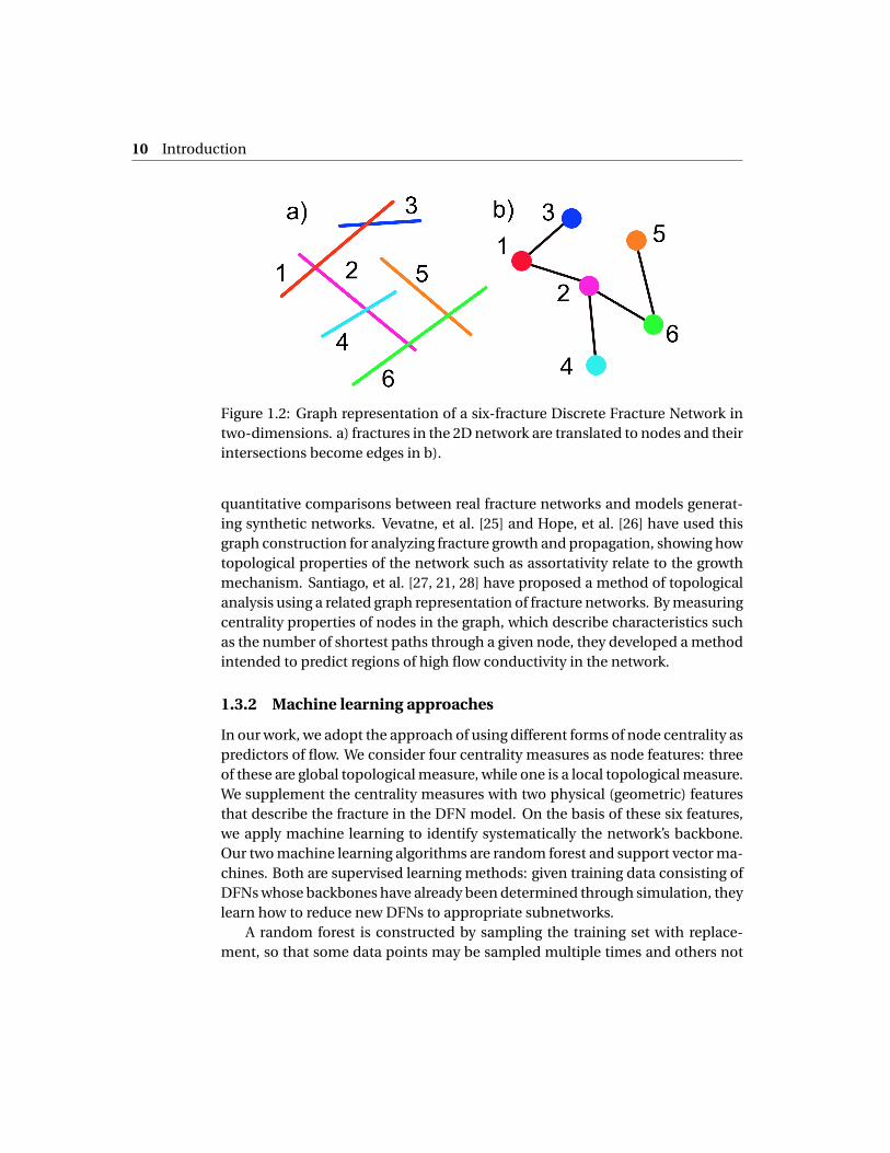
Our approach is based on representing a given DFN by a graph, where a nodein the graph represents a fracture in the network, and an edge connecting twonodes in the graph represents an intersection between two fractures. Under thisconstruction, the graph retains topological information about the network asnode-based properties or features. An example of representing a DFN by a graphis given in Figure 1.2 for a two-dimensional six-fracture network.

Such a graph representation was proposed by Ghaffari, et al. [23] and inde-pendently by Andresen, et al. [24], in order to study the network topology of bothtwo- and three-dimensional fracture systems. The graph mapping allowed fora characterization of the topology of fracture networks, and moreover enabled

10 Introduction

Figure 1.2: Graph representation of a six-fracture Discrete Fracture Network intwo-dimensions. a) fractures in the 2D network are translated to nodes and theirintersections become edges in b).

quantitative comparisons between real fracture networks and models generat-ing synthetic networks. Vevatne, et al. [25] and Hope, et al. [26] have used thisgraph construction for analyzing fracture growth and propagation, showing howtopological properties of the network such as assortativity relate to the growthmechanism. Santiago, et al. [27, 21, 28] have proposed a method of topologicalanalysis using a related graph representation of fracture networks. By measuringcentrality properties of nodes in the graph, which describe characteristics suchas the number of shortest paths through a given node, they developed a methodintended to predict regions of high flow conductivity in the network.

1.3.2 Machine learning approaches

In our work, we adopt the approach of using different forms of node centrality aspredictors of flow. We consider four centrality measures as node features: threeof these are global topological measure, while one is a local topological measure.We supplement the centrality measures with two physical (geometric) featuresthat describe the fracture in the DFN model. On the basis of these six features,we apply machine learning to identify systematically the network’s backbone.Our two machine learning algorithms are random forest and support vector ma-chines. Both are supervised learning methods: given training data consisting ofDFNs whose backbones have already been determined through simulation, theylearn how to reduce new DFNs to appropriate subnetworks.

A random forest is constructed by sampling the training set with replace-ment, so that some data points may be sampled multiple times and others not

Project Goals 11

at all. Those data points that are sampled are used to generate a decision tree,which outputs a classification based on feature values. Those data points thatare not sampled are run through the tree to determine its quality. The proce-dure is repeated so as to generate a large collection of trees. A test data pointis then classified by having each decision tree “vote” on its class. This leads notonly to a predicted classification, but also to a measure of certainty (the fractionof trees that voted for it) as well as to an estimate of the importance of each fea-ture [29, 30, 31, 32, 33, 34, 35]. That final estimate is particularly useful when thefeatures consist of quantities that measure different aspects of node centrality.

Support vector machines (SVM) separate high-dimensional data points intotwo classes by finding an appropriate hyperplane. Based on the generalizedportrait algorithm [36] and subsequent developments in statistical learning the-ory [37], the current version of SVM [38] uses kernel methods [39] to generalizelinear classifiers to nonlinear ones. SVMs have been shown to perform well inapplications with highly correlated feature variables, in part because one canchoose kernels or separator boundaries that are most appropriate to the featurespace describing the data [40, 34].

One challenge in the DFN data is the imbalance between the size of the back-bone (“positive”) and non-backbone (“negative”) class. In data from simula-tions, only about 7% of fractures are part of the backbone, reflecting the substan-tial network reduction afforded by the primary flow subnetwork. But this posescomplications in validating our predictions. Simply trying to maximize the over-all rate of correct classification could result in labeling much of the backbone asnon-backbone (false negative), in which case the flow properties of the reducednetwork would not match those of the original. We therefore consider both pre-cision (ratio of true positives to all positives) and recall (ratio of true positivesto true positive plus false negatives). There is a trade-off between these two,controlled by how strict the classifier is in labeling a sample as positive. Whileour primary objective is recall, so as to minimize false negatives that can ob-struct flow, we are also concerned with exploring the precision/recall space. Wetherefore use a grid search method that identifies classifier parameters criticalto precision and recall. By modifying these parameters, we evaluate how far weare able to reduce the network without significantly affecting flow.

It is important to note that our objective is flow-maintaining network re-duction, which is not identical to predicting the backbones determined fromparticle-based simulation. While we use these backbones as training data forour classifiers, the main validation of our results comes through considering thebreakthrough curve (BTC). This curve shows the distribution of simulated par-ticles passing through the network from source plane to target plane in a giveninterval of time. We would like the BTC for our reduced networks to match that

12 Introduction

of the full network in a number of respects, including peak breakthrough time,and the nature of the tail of the distribution. While the particle backbone is im-portant for identifying where mass transports through the network, it is only oneof many valid network reductions from the perspective of characterizing flow.

We find that, under different parameter choices for random forest and SVM,we are able to reduce DFNs on average to between 39% and 2.5% of their orig-inal number of fractures. The two extremes correspond to recall values of 96%and 20%. Reductions to as little as 21% (with recall of 75%) provide good BTCmatches, with Kolmogorov-Smirnov statistic values of 0.26 or less. We also as-sess the importance of the different features used to characterize the data, find-ing that they cluster into three natural groups. The global topological quantitiesare the most significant ones, followed by the one local topological quantity weuse. The physical quantities are the least significant ones, though still necessaryfor the performance of the classifier. A manuscript describing our work and theresults above has been submitted for publication [17].

We consider a further classification approach that, based on initial tests,not only provides significant network reduction but also comes closer to re-constructing the particle backbone itself. This is a two-stage method, whichfirst forms an initial classification of nodes next to the source and to the sink,and then attempts to propagate labels from nodes identified as backbone. Themethod was originally motivated by the observation that straightforward appli-cations of random forest and SVM, as described above, can result in backbonesthat do not connect to both the source and sink. Clearly, such disconnectedstructures are not usable as a flow subnetwork. In reality, the problem only oc-curs at parameter choices giving very low recall. But even there, the two-stagemethod almost always gives a connected backbone. At parameter choices giv-ing high recall, the two-stage method appears to provide outstanding reduction,yielding a subnetwork with only 17% of the original number of fractures whilemaintaining 90% recall. This method merits further study and development.

1.3.3 Dynamic problem

Finally, we investigate the dynamic problem of modeling fracture growth, andof predicting material failure using machine learning techniques. A number ofrecent studies have considered modeling crack propagation using a set of rulesthat act directly on the graph representing the fracture network [25, 26, 18, 41,42]. To understand this process, consider a fracture with multiple intersections,modeled as a node in a graph with multiple neighbors. Fracture networks havebeen found to exhibit strong negative correlations in the degree of neighboringnodes; there is a tendency for nodes of high degree (many neighbors) to con-

Project Goals 13

nect to nodes of low degree (few neighbors) and vice versa. Such networks arecalled disassortative. The strong correlations lend credence to the idea that newfractures depend heavily on the existing network, and that the growth process issimilar to a preferential growth mechanism, where new nodes are more likely tocouple to existing nodes of high degree. Note that node degree may or may notbe the best metric to utilize for preferential growth; for example, Vevatne et al.[25] use the lengths of existing fractures as the growth metric. We present a pre-liminary study of fracture growth using a basic random graph model, and sug-gest improvements to this model. We also discuss promising methods for rapidprediction of material failure, using classification based on topological and geo-metric features.

Chapter 2

Classification Methods

Given a set of features and class assignment for some observations, supervisedlearning algorithms try to “learn” the underlying function that maps features toclasses. Those observations are the training set. The learned function can thenbe used to classify new observations. In our study, we use as observations thenodes (fractures) from 80 graphs as a training set. We then test the functionusing nodes from 20 graphs as a test set.

One challenge we face is a significant imbalance in the number of observa-tions in each class. For the 80 graphs in the training set, only about 7 percentof nodes are part of the backbone class. A classification algorithm could simplyassign all nodes to the non-backbone class, and still achieve an overall classifi-cation accuracy of 93 percent. Since our aim is to find a meaningful backbone,careful attention must be given to identifying the parameters of our algorithmsthat maximize the recall, or fraction of backbone nodes in the training set thatare correctly predicted.

In this chapter, we describe the features that we use to describe nodes, andour machine learning methods based on random forests and support vector ma-chines. Both are general-purpose supervised learning methods that are suitableboth geometric as well as non-geometric features. Furthermore, while both ofthese algorithms are highly tunable, they rarely require very extensive parametertuning. We discuss our process for parameter selection, and how we use this toinvestigate the tradeoff between network reduction and accuracy of flow proper-ties. Both algorithms are implemented using the scikit-learn machine learningpackage in python, with the functions RandomForestClassifier and SVC.

16 Classification Methods

2.1 Node Features

It may seem that the most natural way to identify a flow subnetwork is to con-sider all possible source-to-sink paths, and to predict which of those are partof the backbone. This approach, however, is impractical due to the exponen-tial proliferation of possible paths. Instead, we consider individual nodes, andinvestigate features describing these nodes that we expect to be insightful in pre-dicting the backbone.

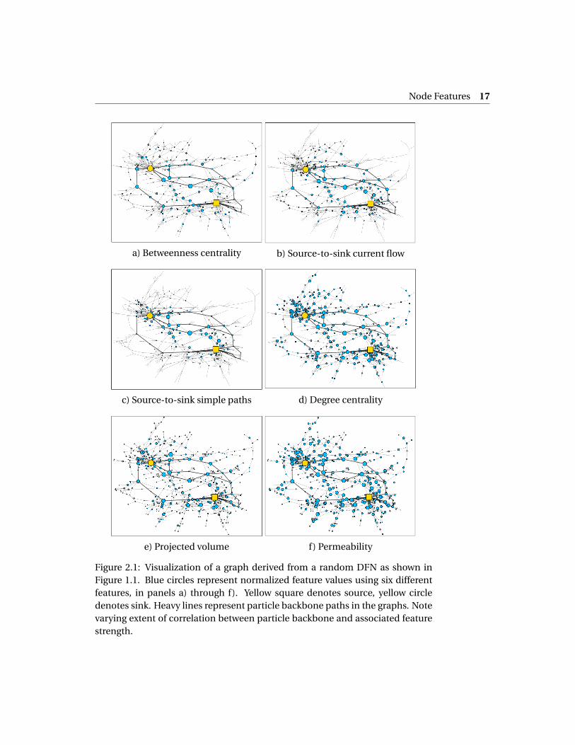
Recent studies suggest that graph-theoretic quantities associated with nodecentrality can help describe crucial topological characteristics of the network [24,25] and identify regions important in conducting flow [21, 28]. Such quantitiescan be divided into two categories: global topological measures, which describea node’s place within a graph structure, and local topological measures, whichdescribe a node’s immediate neighborhood. We expect that both of these canplay a role in predicting the flow properties of a fracture in a network. We there-fore consider features from both categories, calculated using the NETWORKXgraph software package [43]. We also supplement these with a third category offeatures, representing physical properties of the fractures. Figure 2.1 illustratesthe six different features that we choose to describe nodes on a graph represent-ing the DFN shown earlier in Figure 1.1. It shows how feature values relate to thegraph structure and to the particle backbone.

Code for generating the features described below is found on the GitHub sitein the jupyter notebook generate_features.ipynb (see Appendix A).

2.1.1 Global topological features

• The betweenness centrality [44, 45] of a node (Figure 2.1a) reflects the ex-tent to which that node can control communication on a network. Con-sider a geodesic path (path with fewest possible edges) connecting a nodeu and a node v on a graph. In general, there may be more than one suchpath: let σuv denote the number of them. Furthermore, let σuv (i ) denotethe number of such paths that pass through node i . We then define, fornode i ,

Betweenness centrality = 1

(N −1)(N −2)

N∑u,v=1u 6=i 6=v

σuv (i )

σuv, (2.1)

where the leading factor normalizes the quantity so that it can be com-pared across graphs of different size N . Nodes with high betweenness cen-trality might well be expected to have a large influence on transport across

Node Features 17

a) Betweenness centrality b) Source-to-sink current flow

c) Source-to-sink simple paths d) Degree centrality

e) Projected volume f) Permeability

Figure 2.1: Visualization of a graph derived from a random DFN as shown inFigure 1.1. Blue circles represent normalized feature values using six differentfeatures, in panels a) through f). Yellow square denotes source, yellow circledenotes sink. Heavy lines represent particle backbone paths in the graphs. Notevarying extent of correlation between particle backbone and associated featurestrength.


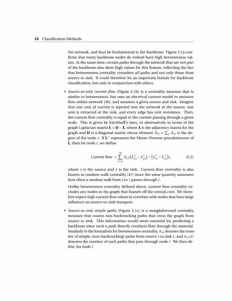
the network, and thus be fundamental to the backbone. Figure 2.1a con-firms that many backbone nodes do indeed have high betweenness val-ues. At the same time, certain paths through the network that are not partof the backbone also show high values for this feature, reflecting the factthat betweenness centrality considers all paths and not only those fromsource to sink. It could therefore be an important feature for backboneclassification, but only in conjunction with others.

• Source-to-sink current flow (Figure 2.1b) is a centrality measure that issimilar to betweenness, but uses an electrical current model to measureflow within network [46], and assumes a given source and sink. Imaginethat one unit of current is injected into the network at the source, oneunit is extracted at the sink, and every edge has unit resistance. Then,the current flow centrality is equal to the current passing through a givennode. This is given by Kirchhoff’s laws, or alternatively in terms of thegraph Laplacian matrix L = D−A, where A is the adjacency matrix for thegraph and D is a diagonal matrix whose element Di i = ∑

j Ai j is the de-gree of the node i . If L+ represents the Moore-Penrose pseudoinverse ofL, then for node i , we define

Current flow =N∑

j=1Ai j |

(L+

i s −L+j s

)− (L+

i t −L+j t

)|, (2.2)

where s is the source and t is the sink. Current-flow centrality is alsoknown as random-walk centrality [47] since the same quantity measureshow often a random walk from s to t passes through i .

Unlike betweenness centrality defined above, current-flow centrality ex-cludes any nodes in the graph that branch off the central core. We there-fore expect high current flow values to correlate with nodes that have largeinfluence on source-to-sink transport.

• Source-to-sink simple paths (Figure 2.1c) is a straightforward centralitymeasure that counts non-backtracking paths that cross the graph fromsource to sink. This information would seem essential for predicting abackbone since such a path directly conducts flow through the material.Similarly to the formalism for betweenness centrality,πst denotes the num-ber of simple (non-backtracking) paths from source s to sink t , and πst (i )denotes the number of such paths that pass through node i . We then de-fine, for node i

Node Features 19

Simple paths = πst (i )

πst, (2.3)

where normalization by πst allows to compare values of simple path cen-trality across different graphs. Since the complexity of path enumerationcan scale exponentially in the size of the graph, we limit our search topaths with 15 nodes or less. This restriction has physical justification, asdirect paths tend to be more common in backbones. While these pathlengths can vary considerably, we find empirically that if we increase theupper bound on path length beyond 15, the effect on the simple path val-ues is negligible.

Figure 2.1c illustrates that nodes with high source-to-sink simple path cen-trality are more likely to lie on backbone paths than are nodes with highbetweenness centrality in Figure 2.1a. However, simple path centralityalso fails to identify one isolated backbone path that is disjoint from theothers. We expect it to serve an important role in backbone classification,though again, only in conjunction with other features.

2.1.2 Local topological feature

• Degree centrality (Figure 2.1d) is a normalized measure of the number ofedges touching a node. For node i ,

Degree centrality = 1

N −1

N∑j=1

Ai j . (2.4)

Nodes with high degree centrality tend to be concentrated in the core ofthe network. Conversely, nodes with low degree centrality are often in theperiphery or on branches that cannot possibly conduct significant flow.Furthermore, since the degree centrality of a fracture is the number ofother fractures that intersect with it, degree centrality is closely related tofracture volume.

2.1.3 Physical features

We supplement the four topological features with two features describing phys-ical and geometric properties of fractures.

• Projected volume (Figure 2.1e) measures the component of a fracture’s vol-ume that is oriented along the direction of flow from inlet to outlet plane.


Fracture planes have different orientations in the DFN, and those that areoriented parallel to the main flow direction are more likely to conduct sig-nificant flow than those that are oriented perpendicular the normal flowdirection. We therefore consider the projection of the volume onto theaxis of flow. Let fracture i have volume Vi and orientation vector Oi (unitvector normal to the fracture plane). Taking the flow to be oriented alongthe x-axis, the projected volume is expressed in terms of the projection ofOi onto the y z-plane:

Projected volume =Vi

√(Oi )2

y + (Oi )2z . (2.5)

Figure 2.1e shows similarities between this feature and degree centrality,but also some fractures where one feature correlates more closely with thebackbone than the other.

• Permeability (Figure 2.1f) measures how easily a porous medium allowsflow. Given the aperture size bi of fracture i , the permeability is expressedas

Permeability = b2i

12(2.6)

The permeability of a fracture, which is nonlinearly related to its volume,is a further measure of its transport capacity. As illustrated in Figure 2.1, itdisplays similarities to both degree centrality and projected volume, withbackbone fractures almost systematically having high permeability values(but the converse holding less consistently).

2.1.4 Correlation of feature values

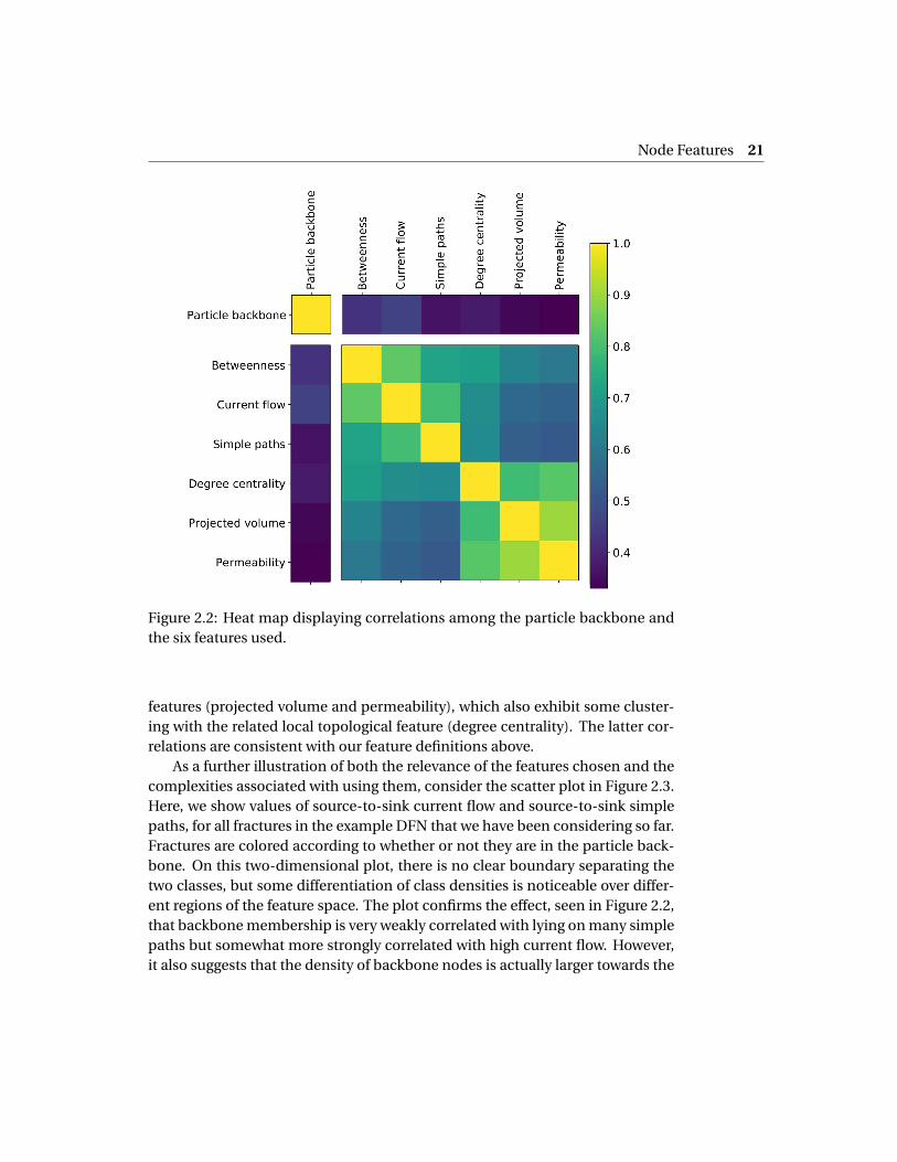
As is seen in Figure 2.1, the feature values vary widely from one node to anotherin ways that we aim to manipulate in order to predict backbone paths. Figure2.2 shows correlation coefficients for pairs that include the particle backboneand the six features that we have chosen. The fact that there are non-negligiblecorrelations between the backbone and these features suggests that they are rel-evant ones for classification, although clearly no single feature is sufficient initself. We also notice from the correlation coefficients that features tend to clus-ter naturally into the three categories above. The first three features, which arethe global topological ones (betweenness, current flow, and simple paths), havesignificant mutual correlations among then. The same is true for the physical

Node Features 21

Figure 2.2: Heat map displaying correlations among the particle backbone andthe six features used.

features (projected volume and permeability), which also exhibit some cluster-ing with the related local topological feature (degree centrality). The latter cor-relations are consistent with our feature definitions above.

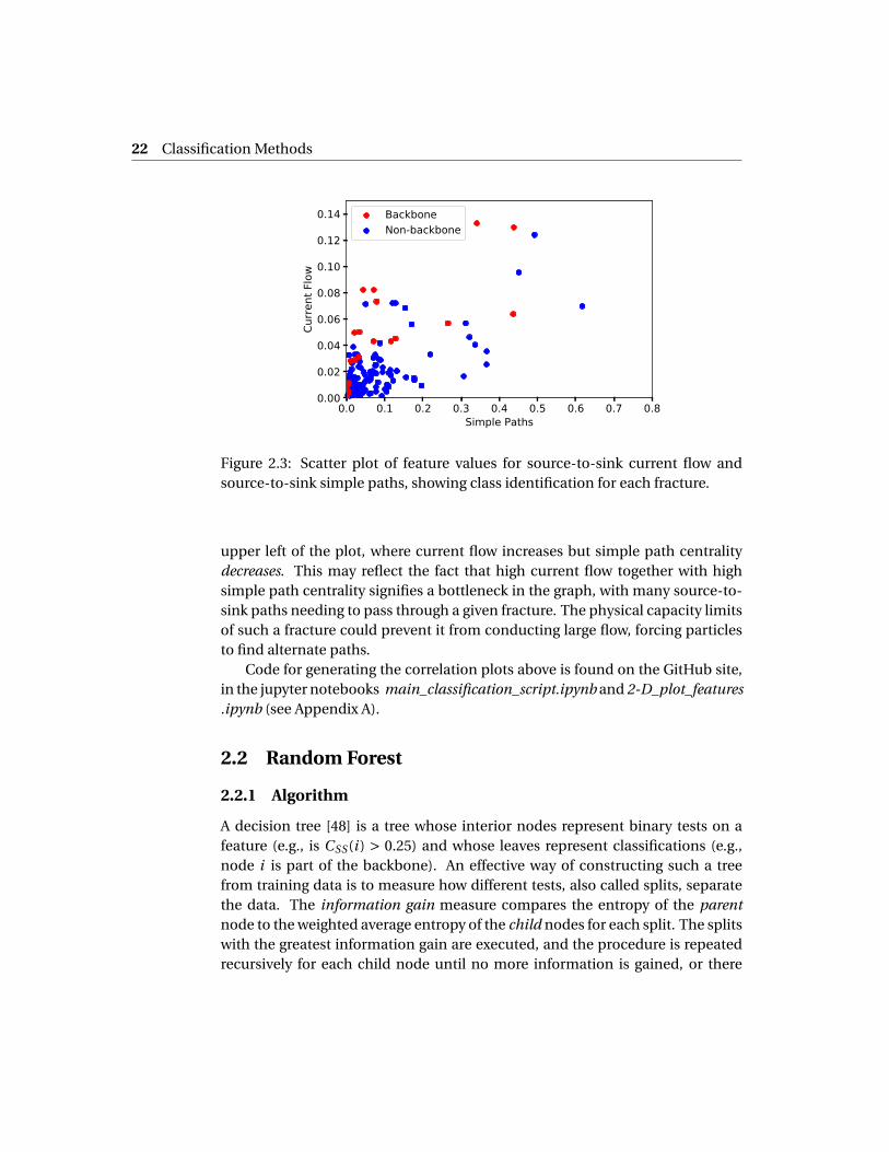
As a further illustration of both the relevance of the features chosen and thecomplexities associated with using them, consider the scatter plot in Figure 2.3.Here, we show values of source-to-sink current flow and source-to-sink simplepaths, for all fractures in the example DFN that we have been considering so far.Fractures are colored according to whether or not they are in the particle back-bone. On this two-dimensional plot, there is no clear boundary separating thetwo classes, but some differentiation of class densities is noticeable over differ-ent regions of the feature space. The plot confirms the effect, seen in Figure 2.2,that backbone membership is very weakly correlated with lying on many simplepaths but somewhat more strongly correlated with high current flow. However,it also suggests that the density of backbone nodes is actually larger towards the


0.0 0.1 0.2 0.3 0.4 0.5 0.6 0.7 0.8Simple Paths

0.00

0.02

0.04

0.06

0.08

0.10

0.12

0.14

Curre

nt F

low

BackboneNon-backbone

Figure 2.3: Scatter plot of feature values for source-to-sink current flow andsource-to-sink simple paths, showing class identification for each fracture.

upper left of the plot, where current flow increases but simple path centralitydecreases. This may reflect the fact that high current flow together with highsimple path centrality signifies a bottleneck in the graph, with many source-to-sink paths needing to pass through a given fracture. The physical capacity limitsof such a fracture could prevent it from conducting large flow, forcing particlesto find alternate paths.

Code for generating the correlation plots above is found on the GitHub site,in the jupyter notebooks main_classification_script.ipynb and 2-D_plot_features.ipynb (see Appendix A).

2.2 Random Forest

2.2.1 Algorithm

A decision tree [48] is a tree whose interior nodes represent binary tests on afeature (e.g., is CSS(i ) > 0.25) and whose leaves represent classifications (e.g.,node i is part of the backbone). An effective way of constructing such a treefrom training data is to measure how different tests, also called splits, separatethe data. The information gain measure compares the entropy of the parentnode to the weighted average entropy of the child nodes for each split. The splitswith the greatest information gain are executed, and the procedure is repeatedrecursively for each child node until no more information is gained, or there

Random Forest 23

are no more possible splits. A limitation of decision trees is that the topologyis completely dependent on the training set, Variations in the training data canproduce substantially different trees.

The random forest method [49, 50] addresses this problem by constructing acollection of trees using subsamples of the training data. These subsamples aregenerated with replacement (bootstrapping), so that some data points are sam-pled more than once and some not at all. The sampled “in-bag” data points areused to generate a decision tree. The “out-of-bag” observations (the ones notsampled) are then run through the tree to estimate its quality [29]. This proce-dure is repeated to generate a large number (hundreds or thousands) of randomtrees. To classify a test data point, each tree “votes” for a result. This provides notonly a predicted classification, determined by majority rule, but also a measureof certainty, determined by the fraction of votes in favor. The use of bootstrap-ping effectively augments the data, allowing random forest to perform well usingfewer features than other methods.

Additionally, random forest provides an estimate of how important each in-dividual feature is for the class assignment. This is calculated by permuting thefeature’s values, generating new trees, and measuring the “out-of-bag” classifi-cation errors on the new trees. If the feature is important for classification, thesepermutations will generate many errors. If the feature is not important, they willhardly affect the performance of the trees.

Code for running the random forest algorithm is found on the GitHub site inthe jupyter notebook main_classification_script.ipynb (see Appendix A).

2.2.2 Parameter Selection

In order to identify the parameters of random forest that affect our results mostsignificantly, we use a grid search cross-validation method, implemented withthe GridSearchCV function in scikit-learn. This method optimizes a classifier byexhaustive search within a given range of parameter values, recursively build-ing and testing models. Given the class imbalance in our problem, we set theparameter ranges to aim for high recall. We find the greatest sensitivity to a pa-rameter that sets the minimal number of samples in a leaf node. This parameterforces the algorithm to reject any candidate split that would result in a childnode having fewer than a fixed number of observations. Adjusting that numbercan prevent overfitting, which in the context of unbalanced classes could causepractically none of the feature space to be assigned to the minority class.

Another important parameter choice involves class weights. When randomforest classifies a new observation, and the observation ends up in a leaf nodewith training observations from more than one class, that particular tree will


output a fractional vote for a class according to the number of training obser-vations of that class in the leaf. One often sets all training observations to haveequal weights. However, by instead assigning training observations a weight thatis inversely proportional to class frequency, so that votes from the minority classcount more, we can effectively move the decision boundary in favor of a back-bone classification.

Additional code for random forest parameter selection is found on the Git-Hub site in the jupyter notebook model_selection.ipynb (see Appendix A).

2.3 Support Vector Machines

2.3.1 Algorithm

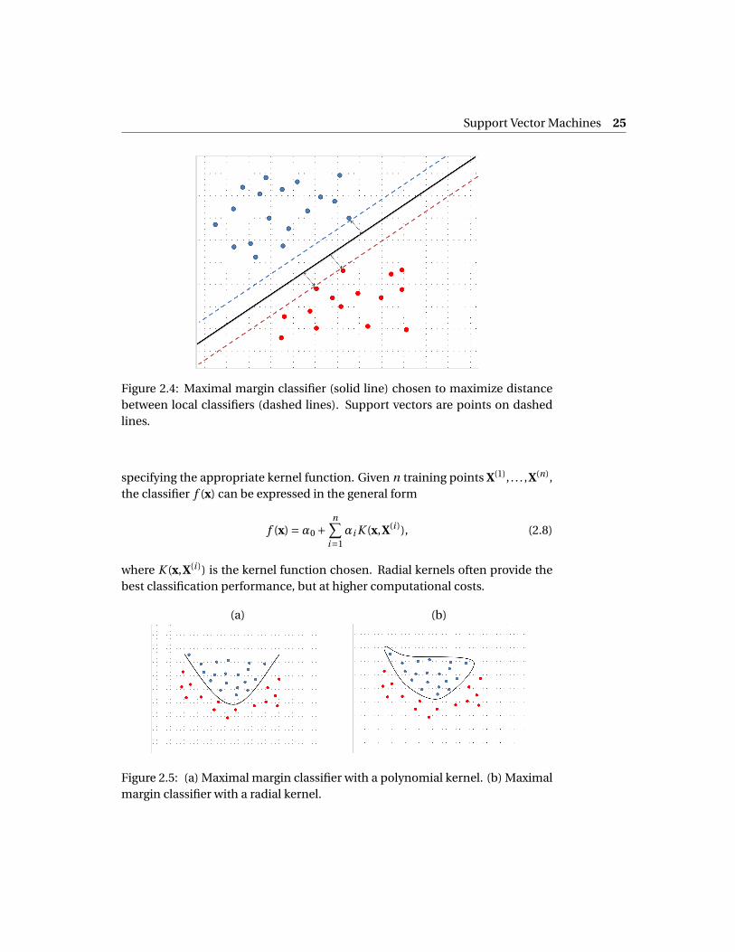
Support vector machines (SVM) use a maximal margin classifier to perform bi-nary classification. Given training data described by p features, the methodidentifies boundary limits for each class in the p-dimensional feature space.These boundary limits, which are (p −1)-dimensional hyperplanes, are knownas local classifiers, and the distance between the local classifiers is called themargin. SVM attempts to maximize this margin, making the data as separableas possible, and defines the classifier as a hyperplane in the middle that sepa-rates the data into two groups. The data points on the boundaries are called sup-port vectors, since they “support” the limits and define the shape of the maximalmargin classifier. An example for two features (p = 2) is shown in Figure 2.4.

Once SVM has generated a maximal margin classifier from training data, oneuses this to predict the class of test data points. For example, given p features,the classifier for a linear kernel can be written as:

f (x) =β0 +p∑

j=1β j x j , (2.7)

where x is a vector whose j th component x j represents the value of the testpoint’s j th feature, and the parameters β j are derived from the training data.The point is assigned to one class if f (x) < 0, and to the other if f (x) > 0. Inthe p = 2 example of Figure 2.4, any test point lying on the left of the solid linewould be assigned to the blue class and any test point lying on the right wouldbe assigned to the red class.

SVM falls into the category of kernel methods, a theoretically powerful andcomputationally efficient means of generalizing linear classifiers to nonlinearones. For instance, on a two-dimensional surface, instead of a straight line wecan choose a polynomial curve (Figure 2.5a) or a radial loop (Figure 2.5b), by

Support Vector Machines 25

Figure 2.4: Maximal margin classifier (solid line) chosen to maximize distancebetween local classifiers (dashed lines). Support vectors are points on dashedlines.

specifying the appropriate kernel function. Given n training points X(1), . . . ,X(n),the classifier f (x) can be expressed in the general form

f (x) =α0 +n∑

i=1αi K (x,X(i )), (2.8)

where K (x,X(i )) is the kernel function chosen. Radial kernels often provide thebest classification performance, but at higher computational costs.

(a) (b)

Figure 2.5: (a) Maximal margin classifier with a polynomial kernel. (b) Maximalmargin classifier with a radial kernel.


There are a number of practical considerations in feature selection for SVM.First of all, we follow the usual practice of standardizing the data set as a prepro-cessing step. This involves rescaling each feature so that values have mean zeroand variance one, thereby eliminating distortions that could bias the classifier infavor of a given feature. Second of all, it is rarely a disadvantage to increase thenumber of features used by SVM, even if those additional features are relativelyunimportant to the class assignment. The maximal margin classifier changesvery little if noisy features are added to the data, making SVM less prone to over-fitting than many other methods. We therefore enhance our feature space forSVM in the following way. For each of the six features discussed in Section 2.1,we rank the values within a given graph: the lowest value within the graph hasrank 1, and so on. Rankings for tied values are arbitrary. We then consider theraw and ranked values as separate features, doubling the size of the feature spacefor both training and prediction.

Code for running the SVM algorithm is found on the GitHub site in the jupyternotebook main_classification_script.ipynb (see Appendix A).

2.3.2 Parameter Selection

The most important parameter affecting the performance of SVM is the toler-ance, known as C . In order to avoid overfitting, SVM often uses a “soft” mar-gin rather than a hard one, allowing misclassification among the training data.When C is set to be large, tolerance is low: C →∞ is the limiting case of the hardmargin described above, where local classifiers strictly bound data points fromone class. When C is small, tolerance is high: a training point from one classmay be found on either side of the local classifier.

As in the case of random forest, we use grid search cross-validation to iden-tify and optimize crucial parameters such as tolerance. Due to the class imbal-ance in the problem, it is necessary to adjust the weights associated with theclasses. Rather than setting the same tolerance value, C , for both classes, we as-sign a weight to the tolerance for each class. This allows the local classifier tomore strictly bound the (minority) backbone nodes rather than the (majority)non-backbone nodes. In this way, we can prevent the classifier from overfittingthe majority class while simultaneously preventing it from missing points in theminority class. Using different weights allows us to construct classifiers that aremore likely or less likely to assign a node to the backbone class.

Additional code for SVM parameter selection is found on the GitHub site inthe jupyter notebook model_selection.ipynb (see Appendix A).

Two-Stage Method 27

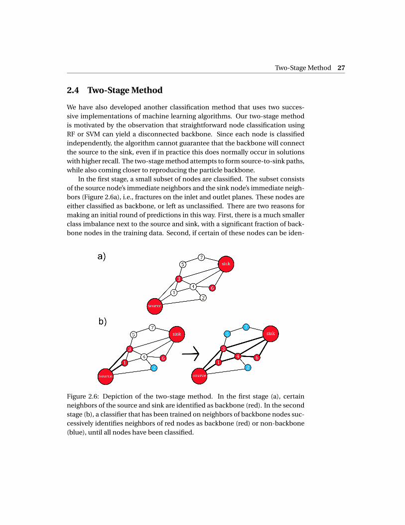
2.4 Two-Stage Method

We have also developed another classification method that uses two succes-sive implementations of machine learning algorithms. Our two-stage methodis motivated by the observation that straightforward node classification usingRF or SVM can yield a disconnected backbone. Since each node is classifiedindependently, the algorithm cannot guarantee that the backbone will connectthe source to the sink, even if in practice this does normally occur in solutionswith higher recall. The two-stage method attempts to form source-to-sink paths,while also coming closer to reproducing the particle backbone.

In the first stage, a small subset of nodes are classified. The subset consistsof the source node’s immediate neighbors and the sink node’s immediate neigh-bors (Figure 2.6a), i.e., fractures on the inlet and outlet planes. These nodes areeither classified as backbone, or left as unclassified. There are two reasons formaking an initial round of predictions in this way. First, there is a much smallerclass imbalance next to the source and sink, with a significant fraction of back-bone nodes in the training data. Second, if certain of these nodes can be iden-

Figure 2.6: Depiction of the two-stage method. In the first stage (a), certainneighbors of the source and sink are identified as backbone (red). In the secondstage (b), a classifier that has been trained on neighbors of backbone nodes suc-cessively identifies neighbors of red nodes as backbone (red) or non-backbone(blue), until all nodes have been classified.


tified as positive (backbone) with high accuracy, then it may be easier to obtainaccurate predictions of how flow propagates further through the network.

The second stage addresses precisely the flow propagation problem, but usesa different classifier that is trained explicitly on neighbors of backbone nodes.The algorithm starts from the nodes identified as backbone in the first stage, andconsiders their neighbors, classifying them as backbone or non-backbone (Fig-ure 2.6b, left). It then successively repeats this process on neighbors of nodes al-ready classified as backbone, thereby generating backbone paths, until all nodeshave been classified (Figure 2.6b, right). This almost always results in a con-nected source-to-sink backbone. If it does not, a connected backbone can beenforced by requiring that at each step, at least one previously unclassified neigh-bor is classified as backbone. Physically, this is similar to forcing flow to continuepropagating from backbone nodes.

In order to lower the rate of false positives, the algorithm uses an enhancedspace of ranked features. For the first stage, this consists of precisely the six rawand six ranked features used for the SVM implementation in Section 2.3. For thesecond stage, however, in addition to these twelve, the algorithm also considerranked feature values where the ranking is determined only among neighborsof a given node. By doing so, it attempts to mimic the flow options availableto particles at a given fracture, incorporating the simultaneous use of local andglobal information to predict how flow propagates.

For both the first and second stages, either RF or SVM may be used. Thesame method does not necessarily need to be used in both stages: different com-binations may be tried. Our implementation uses RF in both stages, and the firststage employs the identical algorithm to that of section 2.2. However, the use ofthe two-stage method results in considerably improved precision and recall, asdiscussed below in section 3.5.

Code for running the two-stage algorithm is found on the GitHub site in thejupyter notebook two_stage.ipynb (see Appendix A).

2.5 Dynamic Graph

We briefly considered the separate problem of fracture growth and propagation,for predicting failure in brittle materials. The nature of the classification prob-lem here is quite different from the static problem of backbone identificationthat was our primary focus.

The first challenge is simply to develop a set of basic rules that model frac-ture growth and material failure, understood as the moment when a failure planedevelops in the network. We use a straightforward dynamic graph model, moti-

Dynamic Graph 29

vated by random geometric graphs, and similar in some respects to the recentlyproposed random neighborhood graph model [42]. We start with a collectionof nodes placed uniformly at random in a unit square. These nodes represent“seeds” that subsequently grow into fractures. Initially, no edges exist. As the dy-namic graph evolves, edges are added, representing the increasing intersectionof planes due to fracture growth. Eventually, a connected path of edges spansthe graph from one boundary to the opposite boundary, representing a failureplane. The time it takes for this plane to appear is called failure time, and themethod used to attach edges in the graphs are a set of basic rules that emulatestress applied in the material, to make the fractures grow and coalesce. Differentsets of rules have been applied in the literature [51, 25, 26].

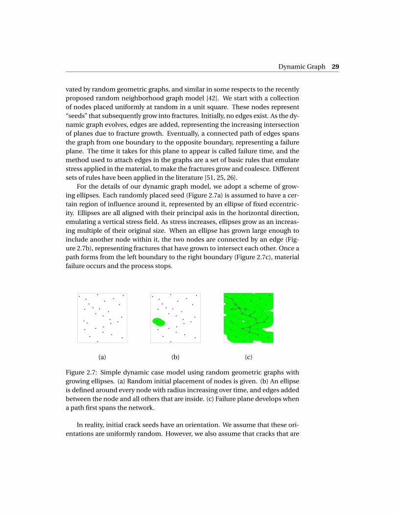
For the details of our dynamic graph model, we adopt a scheme of grow-ing ellipses. Each randomly placed seed (Figure 2.7a) is assumed to have a cer-tain region of influence around it, represented by an ellipse of fixed eccentric-ity. Ellipses are all aligned with their principal axis in the horizontal direction,emulating a vertical stress field. As stress increases, ellipses grow as an increas-ing multiple of their original size. When an ellipse has grown large enough toinclude another node within it, the two nodes are connected by an edge (Fig-ure 2.7b), representing fractures that have grown to intersect each other. Once apath forms from the left boundary to the right boundary (Figure 2.7c), materialfailure occurs and the process stops.

(a) (b) (c)

Figure 2.7: Simple dynamic case model using random geometric graphs withgrowing ellipses. (a) Random initial placement of nodes is given. (b) An ellipseis defined around every node with radius increasing over time, and edges addedbetween the node and all others that are inside. (c) Failure plane develops whena path first spans the network.

In reality, initial crack seeds have an orientation. We assume that these ori-entations are uniformly random. However, we also assume that cracks that are


perpendicular to the stress field will propagate the fastest, whereas cracks thatare parallel to the stress field will not propagate at all. Therefore, we take a seed’soriginal ellipse size to be proportional to the projection of the orientation vector(orthogonal to the crack) onto the stress axis.

Code for the dynamic graph simulation is found on the GitHub site in thejupyter notebook dynamic_graph.ipynb (see Appendix A).

The larger challenge is prediction and classification. While running this codeis computationally trivial, running more realistic crack propagation simulationscan exhaust computational resources. The intention is therefore to use our ran-dom model and related ones to form a testbed for predicting failure paths, usingmachine learning. Ideally, we want to identify fractures that lie on the failurepath without having to run the simulation, and purely from features associatedwith the fracture topology and geometry. Identifying the failure path has similar-ities to identifying a flow backbone, but the relevant features are hardly straight-forward. There is no clear definition of node centrality in the initial graph, be-cause initially there are no edges. The distance from a node to its nearest neigh-bor may be a predictor for classification. More likely, however, one needs toconsider distances to the kth neighbor, with k > 1, in order to capture the globalinformation needed to predict failure.

Chapter 3

Results

We used a collection of 100 graphs, 80 of which were chosen as training data,and 20 of which were chosen as test data. We illustrate certain results, includingbreakthrough curves, on the DFN shown in Figure 1.1. Other results are basedon the entire test set, which consists of a total of 9238 fractures, 651 of which(7.0%) are in the particle backbone and 8587 of which (93%) are not. The totalcomputation time to train both RF and SVM was on the order of a minute, negli-gible compared to the time to extract the particle backbone needed for training.Once trained, the classifier ran on each test graph in seconds.

3.1 Performance Measures

We define a positive classification of a node as being an assignment to the back-bone class, and a negative classification as being an assignment to the non-backbone class. True positives (TP) and true negatives (TN) represent nodeswhose backbone or non-backbone assignment matches that of the labeled train-ing data. False positives (FP) and false negatives (FN) represent nodes whosebackbone or non-backbone assignment is opposite that of the labeled trainingdata. Therefore, one straightforward measure of success is the TP rate. Precisionand recall represent two kinds of TP rates:

Precision = T P

T P +F P(3.1)

Recall = T P

T P +F N(3.2)

Notice that precision is the number of true positives over the total numberthat we classify as positive, whereas recall is the number of true positives over

32 Results

the total number of actual positives. These values give an understanding of howreliable (precision) and complete (recall) our results are.

Note, however, that even though we train our classifier according to the par-ticle backbone, our objective is not necessarily a perfect recovery of that struc-ture. We aim to identify fractures that are a small subset of the full network, butnevertheless conduct significant flow and provide good agreement with the fullnetwork’s breakthrough curve. Many, but not all, of the fractures in the parti-cle backbone are essential for this purpose. Thus, high recall is needed, thoughnot necessarily perfect recall. Precision is less essential: false positives will in-crease the size of our remaining network, but even low precision could allow fora significant reduction in the number of fractures. While we hope to reduce thenetwork while still maintaining flow properties, we also wish to study the trade-off between these two goals.

3.2 Random Forest

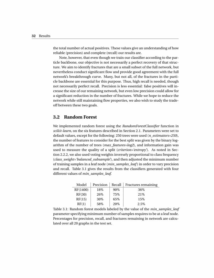
We implemented random forest using the RandomForestClassifier function inscikit-learn, on the six features described in Section 2.1. Parameters were set todefault values, except for the following: 250 trees were used (n_estimators=250),the number of features to consider for the best split was given by the binary log-arithm of the number of trees (max_features=log2), and information gain wasused to measure the quality of a split (criterion=‘entropy’). As noted in Sec-tion 2.2.2, we also used voting weights inversely proportional to class frequency(class_weight=‘balanced_subsample’), and then adjusted the minimum numberof training samples in a leaf node (min_samples_leaf ) in order to vary precisionand recall. Table 3.1 gives the results from the classifiers generated with fourdifferent values of min_samples_leaf.

Model Precision Recall Fractures remainingRF(1400) 18% 90% 36%

RF(30) 26% 75% 21%RF(15) 30% 65% 15%RF(1) 58% 20% 2.5%

Table 3.1: Random forest models labeled by the value of the min_samples_leafparameter specifying minimum number of samples requires to be at a leaf node.Percentages for precision, recall, and fractures remaining in network are calcu-lated over all 20 graphs in the test set.

Random Forest 33

Curre

nt fl

ow

Sim

ple

path

s

Betw

eenn

ess

Degr

ee c

entr

Perm

eabi

lity

Proj

vol

ume0.0

0.1

0.2

0.3

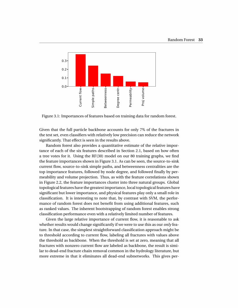
Figure 3.1: Importances of features based on training data for random forest.

Given that the full particle backbone accounts for only 7% of the fractures inthe test set, even classifiers with relatively low precision can reduce the networksignificantly. That effect is seen in the results above.

Random forest also provides a quantitative estimate of the relative impor-tance of each of the six features described in Section 2.1, based on how oftena tree votes for it. Using the RF(30) model on our 80 training graphs, we findthe feature importances shown in Figure 3.1. As can be seen, the source-to-sinkcurrent flow, source-to-sink simple paths, and betweenness centralities are thetop importance features, followed by node degree, and followed finally by per-meability and volume projection. Thus, as with the feature correlations shownin Figure 2.2, the feature importances cluster into three natural groups. Globaltopological features have the greatest importance, local topological features havesignificant but lower importance, and physical features play only a small role inclassification. It is interesting to note that, by contrast with SVM, the perfor-mance of random forest does not benefit from using additional features, suchas ranked values. The inherent bootstrapping of random forest enables strongclassification performance even with a relatively limited number of features.

Given the large relative importance of current flow, it is reasonable to askwhether results would change significantly if we were to use this as our only fea-ture. In that case, the simplest straightforward classification approach might beto threshold according to current flow, labeling all fractures with values abovethe threshold as backbone. When the threshold is set at zero, meaning that allfractures with nonzero current flow are labeled as backbone, the result is simi-lar to dead-end fracture chain removal common in the hydrology literature, butmore extreme in that it eliminates all dead-end subnetworks. This gives per-

34 Results

fect (100%) recall, since all fractures in the particle backbone necessarily havenonzero current flow, and 15% precision, reducing the network to 50% of itsoriginal size. However, difficulties occur when increasing the threshold. Whilethe precision and recall results (discussed below and in Figure 3.2) are in somecases competitive with RF, the backbone itself stops being a connected struc-ture and loses its physical relevance. By contrast, with the exception of the low-recall case of RF(1), our multiple-feature classification methods always maintaina connected backbone in spite of the fact that they classify fractures rather thanpaths.

Just as one can vary the current-flow threshold to produce different preci-sion/recall outcomes, one can adjust a given classifier. Note that this is not thesame as generating different classifiers from the training data, as we do in Ta-ble 3.1. Instead, we take a trained classifier, and modify it to give more or fewerpositive assignments. By default, random forest assigns a node to the class re-ceiving at least 50% of the (weighted) tree votes. Changing this threshold willchange the number of positive assignments. A low voting threshold will result inhigh recall (few false negatives) but low precision (many false positives). A highthreshold will result in low recall (many false negatives) but high precision (fewfalse positives). In this way, by varying an adjustable parameter we can travelalong a precision/recall curve that has perfect recall as one extreme, and perfectprecision as the other.

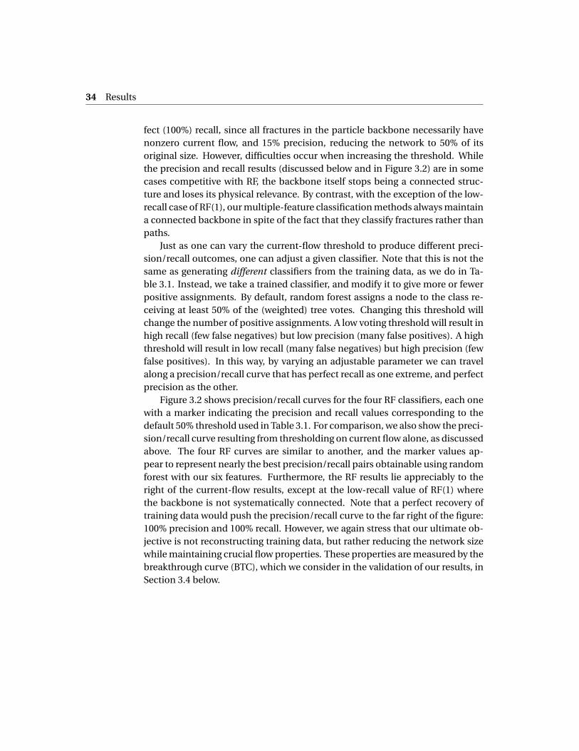
Figure 3.2 shows precision/recall curves for the four RF classifiers, each onewith a marker indicating the precision and recall values corresponding to thedefault 50% threshold used in Table 3.1. For comparison, we also show the preci-sion/recall curve resulting from thresholding on current flow alone, as discussedabove. The four RF curves are similar to another, and the marker values ap-pear to represent nearly the best precision/recall pairs obtainable using randomforest with our six features. Furthermore, the RF results lie appreciably to theright of the current-flow results, except at the low-recall value of RF(1) wherethe backbone is not systematically connected. Note that a perfect recovery oftraining data would push the precision/recall curve to the far right of the figure:100% precision and 100% recall. However, we again stress that our ultimate ob-jective is not reconstructing training data, but rather reducing the network sizewhile maintaining crucial flow properties. These properties are measured by thebreakthrough curve (BTC), which we consider in the validation of our results, inSection 3.4 below.

Support Vector Machine 35

0.0 0.2 0.4 0.6 0.8 1.0Precision

0.0

0.2

0.4

0.6

0.8

1.0Re

call

RF(1400)RF(30)RF(15)RF(1)Current flow

Figure 3.2: Precision/recall curve for the four different random forest classifiersin Table 3.1. Markers indicate default 50% classification threshold for the re-spective model. For comparison, precision/recall curve is also shown based onthresholding on current flow alone.

3.3 Support Vector Machine

We implemented SVM using the SVC function in scikit-learn, on twelve featuresmade of up the six raw features described in Section 2.1 as well as their rankedcounterparts. Parameters were set to their default values, which include a radialkernel, except for those noted in Section 2.3.2. We chose an overall tolerance ofC = 0.01, weighted by additional coefficients (class_weight) for each class thatwe adjusted in order to vary precision and recall. This yields a pair of tolerancesfor the backbone and non-backbone classes. Table 3.2 gives the results from theclassifiers generated with four different pairs of tolerances.

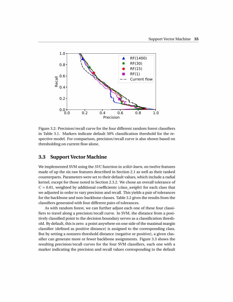
As with random forest, we can further adjust each one of these four classi-fiers to travel along a precision/recall curve. In SVM, the distance from a posi-tively classified point to the decision boundary serves as a classification thresh-old. By default, this is zero: a point anywhere on one side of the maximal marginclassifier (defined as positive distance) is assigned to the corresponding class.But by setting a nonzero threshold distance (negative or positive), a given clas-sifier can generate more or fewer backbone assignments. Figure 3.3 shows theresulting precision/recall curves for the four SVM classifiers, each one with amarker indicating the precision and recall values corresponding to the default

36 Results

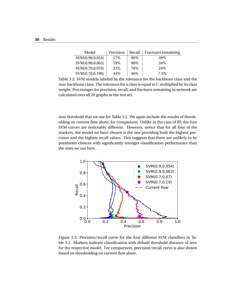
Model Precision Recall Fractures remainingSVM(0.90,0.054) 17% 96% 39%SVM(0.90,0.063) 19% 90% 34%SVM(0.70,0.070) 23% 78% 24%SVM(0.70,0.190) 44% 46% 7.3%

Table 3.2: SVM models labeled by the tolerance for the backbone class and thenon-backbone class. The tolerance for a class is equal to C multiplied by its classweight. Percentages for precision, recall, and fractures remaining in network arecalculated over all 20 graphs in the test set.

zero threshold that we use for Table 3.2. We again include the results of thresh-olding on current flow alone, for comparison. Unlike in the case of RF, the fourSVM curves are noticeably different. However, notice that for all four of themarkers, the model we have chosen is the one providing both the highest pre-cision and the highest recall values. This suggests that there are unlikely to beparameter choices with significantly stronger classification performance thanthe ones we use here.

0.0 0.2 0.4 0.6 0.8 1.0Precision

0.0

0.2

0.4

0.6

0.8

1.0

Reca

ll

SVM(0.9,0.054)SVM(0.9,0.063)SVM(0.7,0.07)SVM(0.7,0.19)Current flow

Figure 3.3: Precision/recall curve for the four different SVM classifiers in Ta-ble 3.2. Markers indicate classification with default threshold distance of zerofor the respective model. For comparison, precision/recall curve is also shownbased on thresholding on current flow alone.

Validation 37

3.4 Validation

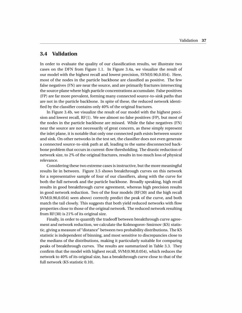
In order to evaluate the quality of our classification results, we illustrate twocases on the DFN from Figure 1.1. In Figure 3.4a, we visualize the result ofour model with the highest recall and lowest precision, SVM(0.90,0.054). Here,most of the nodes in the particle backbone are classified as positive. The fewfalse negatives (FN) are near the source, and are primarily fractures intersectingthe source plane where high particle concentrations accumulate. False positives(FP) are far more prevalent, forming many connected source-to-sink paths thatare not in the particle backbone. In spite of these, the reduced network identi-fied by the classifier contains only 40% of the original fractures.

In Figure 3.4b, we visualize the result of our model with the highest preci-sion and lowest recall, RF(1). We see almost no false positives (FP), but most ofthe nodes in the particle backbone are missed. While the false negatives (FN)near the source are not necessarily of great concern, as these simply representthe inlet plane, it is notable that only one connected path exists between sourceand sink. On other networks in the test set, the classifier does not even generatea connected source-to-sink path at all, leading to the same disconnected back-bone problem that occurs in current-flow thresholding. The drastic reduction ofnetwork size, to 2% of the original fractures, results in too much loss of physicalrelevance.

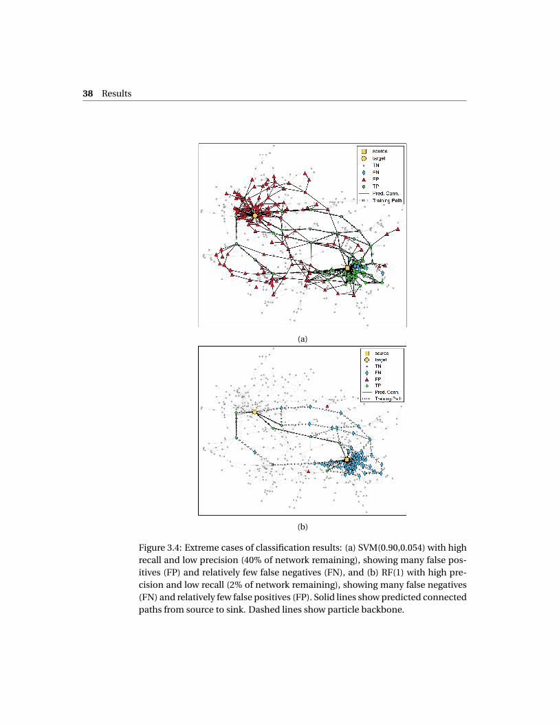
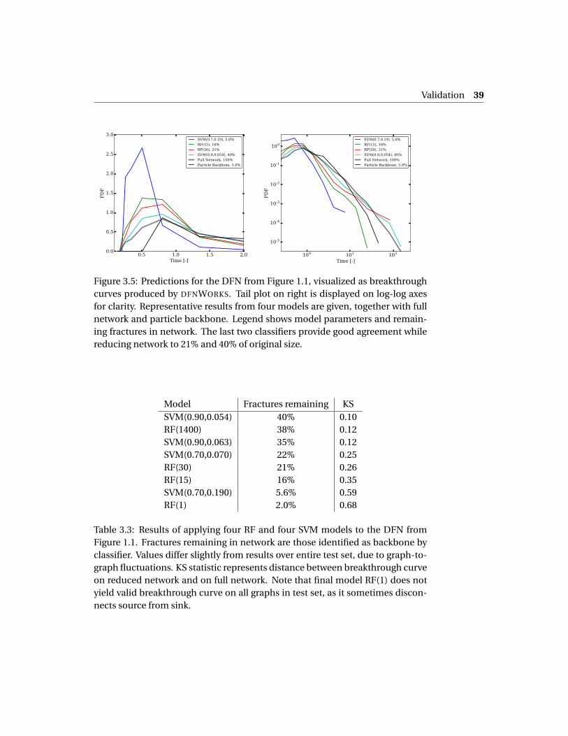
Considering these two extreme cases is instructive, but the more meaningfulresults lie in between. Figure 3.5 shows breakthrough curves on this networkfor a representative sample of four of our classifiers, along with the curve forboth the full network and the particle backbone. Broadly speaking, high recallresults in good breakthrough curve agreement, whereas high precision resultsin good network reduction. Two of the four models (RF(30) and the high recallSVM(0.90,0.054) seen above) correctly predict the peak of the curve, and bothmatch the tail closely. This suggests that both yield reduced networks with flowproperties close to those of the original network. The reduced network resultingfrom RF(30) is 21% of its original size.

Finally, in order to quantify the tradeoff between breakthrough curve agree-ment and network reduction, we calculate the Kolmogorov-Smirnov (KS) statis-tic, giving a measure of “distance” between two probability distributions. The KSstatistic is independent of binning, and most sensitive to discrepancies close tothe medians of the distributions, making it particularly suitable for comparingpeaks of breakthrough curves. The results are summarized in Table 3.3. Theyconfirm that the model with highest recall, SVM(0.90,0.054), which reduces thenetwork to 40% of its original size, has a breakthrough curve close to that of thefull network (KS statistic 0.10).

38 Results

(a)

(b)

Figure 3.4: Extreme cases of classification results: (a) SVM(0.90,0.054) with highrecall and low precision (40% of network remaining), showing many false pos-itives (FP) and relatively few false negatives (FN), and (b) RF(1) with high pre-cision and low recall (2% of network remaining), showing many false negatives(FN) and relatively few false positives (FP). Solid lines show predicted connectedpaths from source to sink. Dashed lines show particle backbone.

Validation 39

0.5 1.0 1.5 2.0Time [-]

0.0

0.5

1.0

1.5

2.0

2.5

3.0

PD

F

SVM(0.7,0.19), 5.6%

RF(15), 16%

RF(30), 21%

SVM(0.9,0.054), 40%

Full Network, 100%

Particle Backbone, 5.6%

100 101 102

Time [-]

10-5

10-4

10-3

10-2

10-1

100

PD

F

SVM(0.7,0.19), 5.6%

RF(15), 16%

RF(30), 21%

SVM(0.9,0.054), 40%

Full Network, 100%

Particle Backbone, 5.6%

Figure 3.5: Predictions for the DFN from Figure 1.1, visualized as breakthroughcurves produced by DFNWORKS. Tail plot on right is displayed on log-log axesfor clarity. Representative results from four models are given, together with fullnetwork and particle backbone. Legend shows model parameters and remain-ing fractures in network. The last two classifiers provide good agreement whilereducing network to 21% and 40% of original size.

Model Fractures remaining KSSVM(0.90,0.054) 40% 0.10RF(1400) 38% 0.12SVM(0.90,0.063) 35% 0.12SVM(0.70,0.070) 22% 0.25RF(30) 21% 0.26RF(15) 16% 0.35SVM(0.70,0.190) 5.6% 0.59RF(1) 2.0% 0.68

Table 3.3: Results of applying four RF and four SVM models to the DFN fromFigure 1.1. Fractures remaining in network are those identified as backbone byclassifier. Values differ slightly from results over entire test set, due to graph-to-graph fluctuations. KS statistic represents distance between breakthrough curveon reduced network and on full network. Note that final model RF(1) does notyield valid breakthrough curve on all graphs in test set, as it sometimes discon-nects source from sink.

40 Results

3.5 Two-Stage Method

Results from the two-stage method are still preliminary. We have not includedthese as part of our validation, and save a more complete study of the methodfor future work. In our preliminary tests, we implemented the algorithm usingrandom forest for both stages, although one could also use SVM for either stage.

For the first stage, we used the identical RF parameters as in Section 3.2,but with 500 trees (n_estimators=500). For the second stage, class imbalance ispractically not an issue, since we are classifying neighbors of backbone nodes.Here, we again used 500 trees (n_estimators=500), and set all other parametersto their default values.

Table 3.4 gives the results from the two-stage classifiers generated with twodifferent values of min_samples_leaf in the first stage, to control precision andrecall. We note that the method is able to achieve, simultaneously, high recalland sufficient precision for significant graph reduction. Our preliminary resultssuggest that this algorithm may provide a large improvement over the results inSections 3.2 and 3.3. Research is ongoing, and fully exploring the potential ofthe two-stage method remains an open challenge.

Model Precision Recall Fractures remainingTwo-Stage(1400) 37% 90% 17%

Two-Stage(1) 45% 82% 13%

Table 3.4: Two-Stage method using random forest in both stages, labeled by thevalue of min_samples_leaf used in the first stage. Percentages for precision, re-call, and fractures remaining in network are calculated over all 20 graphs in thetest set.

3.6 Dynamic Graph

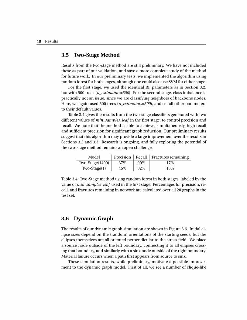
The results of our dynamic graph simulation are shown in Figure 3.6. Initial el-lipse sizes depend on the (random) orientations of the starting seeds, but theellipses themselves are all oriented perpendicular to the stress field. We placea source node outside of the left boundary, connecting it to all ellipses cross-ing that boundary, and similarly with a sink node outside of the right boundary.Material failure occurs when a path first appears from source to sink.

These simulation results, while preliminary, motivate a possible improve-ment to the dynamic graph model. First of all, we see a number of clique-like

Dynamic Graph 41

(a) (b)

Figure 3.6: Results of dynamic graph simulation using growing ellipses. Majoraxes are oriented horizontally and are twice the length of minor axes. (a) Initialellipses are placed randomly, and are of different sizes, depending on randomorientations of associated crack seed. (b) Source node on left connects to all el-lipses crossing left boundary; sink node on right connects to all ellipses crossingright boundary. Failure plane develops when path is created from source to sink.

structures in Figure 3.6b, with edge crossings and highly connected subgraphs.Fracture networks with this topology are unlikely to have straightforward phys-ical interpretations. Second of all, the graph has very few terminal nodes, un-like the structure that we see in, for instance, the DFN from Figure 1.1. In or-der to solve these problems while better modeling the underlying physics ofcrack propagation, one might modify the dynamic graph model in the follow-ing way [52]. Make all edges directed, always oriented from the larger ellipseto the smaller ellipse. The direction of the edge therefore encodes the dynam-ics of which fracture propagates into which other fracture. Furthermore, sincea fracture usually only grows in two direction, limit the number of outgoing di-rected edges from a node to at most two. If two edges already start from a givenfracture, no further directed edges can come out from it, although new directededges can come into it.

Continuing the dynamic graph modeling and implementing a classificationapproach to predicting the failure path remain to be explored as future prob-lems.

Chapter 4

Conclusions

Simulating flow through fractured media is a major computational challenge.The use of discrete fracture networks (DFNs) allows flow to be modeled by par-ticle tracking. Furthermore, one can realize significant computational savingsby identifying a primary flow subnetwork within a DFN, and restricting simula-tion to that backbone subnetwork. However, identifying the backbone by meansof particle simulations is itself too computationally intensive to be practical forlarge networks.

In this clinic project, we have presented a novel approach to finding a back-bone subnetwork that does not require resolving flow in the network, and thattakes minimal computational time. The method involves representing a DFNwith an underlying graph whose nodes represent fractures, and applying ma-chine learning techniques to rapidly predict which nodes are part of the back-bone. We have used two supervised learning techniques: random forest andsupport vector machines. Once these algorithms have been trained on flow datafrom particle simulations, they successfully reduce new DFNs to subnetworksthat preserve crucial flow properties. Our algorithms use topological featuresassociated with nodes on the graph, as well as a small number of physical fea-tures describing a fracture’s properties. We consider each node as a point in themulti-dimensional feature space, and classify it according to whether or not itbelongs to the backbone.

By varying the parameters of our classifiers, we are able to obtain a widerange of precision and recall values. These yield backbones whose sizes rangefrom 40% down to 2% of the original network. For reductions as small as 21%of the original size, the resulting breakthrough curve (BTC) displays good agree-ment with that of the original network. We therefore obtain subnetworks thatare significantly smaller than the full network, useful for flow simulations, and

44 Conclusions

generated in seconds. By comparison, the computation time needed to extractthe particle backbone is on the order of hours.

In addition to the classification results, the random forest method gives aset of relative importances for the features used. These importances are deter-mined by permuting the values of a given feature and observing the effect thishas on classification performance. We have found that features based on globaltopological properties of the underlying graph were significantly more impor-tant than those based on geometry or physical properties of the fractures. Thisreinforces previous observations that network connectivity is more fundamentalto determining flow than are geometric or hydraulic properties [19]. Quantita-tively, the most important of our global topological features is source-to-sinkcurrent flow, which measures how much of a unit of current injected at thesource (representing the inlet plane of the DFN) passes through a given nodeof the graph.

Some evidence suggests that if one could in fact generate backbone pathsrather than backbone nodes, results would improve further. We have developeda two-stage classification method that initially labels fractures at the inlet andoutlet planes, and then successively attempts to propagate fractures labeled asbackbone through the network, thereby forming source-to-sink paths. The ob-jective of this method is to generate subnetworks that are far closer to the parti-cle backbone itself, with the training data used not merely to guide the classifiertoward useful network reductions, but rather in the more conventional machinelearning setting of providing ground truth to be reproduced. Our preliminaryresults suggest that such a method may considerably boost precision and re-call simultaneously, generating subnetworks whose BTC closely matches the fullnetwork but whose size is not much larger than the particle backbone.

Finally, we have performed a preliminary study of the problem of predict-ing fracture propagation under a dynamic graph model. We implemented thisusing a basic random geometric graph with growing ellipses. As these ellipsesgrow and increasingly overlap with each other, edges get added to the graph.Once a path is generated through the graph, from a source node to a sink node,material failure is considered to have occurred. We hope that reduced models ofthis kind can help motivate classification methods that predict the failure pathpurely from initial geometry, without the need for simulations. This challengeremains open.

Appendix A

Code Description

All code developed for the 2016–17 Clinic has been placed on the project Git-Hub site. The code is written in Python, and is primarily organized into jupyternotebooks.

The following information is reproduced from the readme file for the coderepository on GitHub.

A.1 Dependencies

Math clinic scripts require:

• Python 2.7

• networkx 1.11

• numpy 1.12.1

• scikit-learn 0.18.1

• matplotlib 2.0.0

All tests were performed using those versions, but older or newer version ofthe packages might still work.

A.2 Quick start

1. Put the files backbone.txt, connectivity.dat, source.txt, target.txt and vol-ume.txt in transfer/x{i}/ with a different value of {i} for each network.

46 Code Description

2. Put the file permeability.dat in perms/x{i}/ with a different value of {i} foreach network.

3. Put the file {i}vol_proj.txt in vol_proj/ with a different value of {i} for eachnetwork.

4. Run generate_features.ipynb. Make sure to run the last cell twice, chang-ing the value of "norm_rank", once for the raw features, and once for theranked features.

5. Run main_classification_script.ipynb. Make sure to adjust the training/testingproportion in part 2, and the output folder and model in part 10.

A.3 Files

A.3.1 main_classification_script.ipynb

Script that loads all features, trains models on them and produces the confusionmatrices and figures.

A.3.2 clinic_functions.py

Function to read and use the features.

A.3.3 generate_features.ipynb

Script to generate all features from the networks files.

A.3.4 PR_plots.ipynb

Generates the precision recall curves.

A.3.5 dynamic_graph.ipynb

Some code aimed to address the dynamic case.

A.3.6 model_selection.ipynb

Contains several model selection tests.

Folders 47

A.3.7 two_stage.ipynb

Two stage method that uses machine learning on nodes for the first stage andon edges for the second.

A.3.8 2-D_plot_features.ipynb

Generates a 2D plot of features from all graphs

A.3.9 3-D_plot_features.ipynb

Generates a 3D plot of features from all graphs

A.4 Folders

A.4.1 features/

All features for the two_core, current_flow_core and full_graph

A.4.2 norm_rank_features

All ranked features normalized by the number of nodes in its corresponding net-work.

A.4.3 final_results/

Results for all selected models.

A.4.4 transfer/

Raw data on the 100 networks.

A.4.5 figures/

Compendium of all figures done by model selection tests.

A.4.6 graphpositions/

Pickel objects that store the positions of nodes for consistent visualization.

A.4.7 perms/

Raw permeabilities. Needed to compute some features.

48 Code Description

A.4.8 vol_proj/

Volume projection data.

A.4.9 corr_plots/

Correlation plots for BB-NB sets

A.4.10 archive/

Folder that contains old code. For archival purposes.

Bibliography

[1] M. C. Cacas, E. Ledoux, G. de Marsily, B. Tillie, A. Barbreau, E. Durand,B. Feuga, and P. Peaudecerf, “Modeling fracture flow with a stochasticdiscrete fracture network: calibration and validation: 1. the flow model,”Water Resources Research, vol. 26, no. 3, pp. 479–489, 1990. [Online].Available: http://dx.doi.org/10.1029/WR026i003p00479

[2] National Research Council, Rock fractures and fluid flow: contemporaryunderstanding and applications, U. C. on Fracture Characterization andF. Flow, Eds. National Academy Press, 1996.

[3] S. Karra, N. Makedonska, H. Viswanathan, S. Painter, and J. Hyman, “Effectof advective flow in fractures and matrix diffusion on natural gas produc-tion,” Water Resources Research, vol. 51, pp. 1–12, 2014.

[4] J. Hyman, J. Jiménez-Martínez, H. Viswanathan, J. Carey, M. Porter,E. Rougier, S. Karra, Q. Kang, L. Frash, L. Chen, Z. Lei, D. O’Malley, andN. Makedonska, “Understanding hydraulic fracturing: a multi-scale prob-lem,” Phil. Trans. R. Soc. A, vol. 374, no. 2078, p. 20150426, 2016.

[5] C. Jenkins, A. Chadwick, and S. D. Hovorka, “The state of the art in moni-toring and verification—ten years on,” Int. J. Greenh. Gas. Con., vol. 40, pp.312–349, 2015.

[6] J. D. Hyman, S. Karra, N. Makedonska, C. W. Gable, S. L. Painter, andH. S. Viswanathan, “dfnWorks: A discrete fracture network frameworkfor modeling subsurface flow and transport,” Computers and Geosciences,vol. 84, pp. 10–19, 2015. [Online]. Available: http://dx.doi.org/10.1016/j.cageo.2015.08.001

[7] S. Painter and V. Cvetkovic, “Upscaling discrete fracture network simula-tions: An alternative to continuum transport models,” Water Resour. Res.,vol. 41, p. W02002, 2005.

50 Bibliography

[8] S. Painter, V. Cvetkovic, and J.-O. Selroos, “Power-law velocity distributionsin fracture networks: Numerical evidence and implications for tracer trans-port,” Geophys. Res. Lett., vol. 29, no. 14, 2002.

[9] H. Abelin, I. Neretnieks, S. Tunbrant, and L. Moreno, Final report of the mi-gration in a single fracture: experimental results and evaluation. SwedishNuclear Fuel and Waste Management Company, 1985.

[10] H. Abelin, L. Birgersson, L. Moreno, H. Widén, T. Ågren, and I. Neretnieks,“A large-scale flow and tracer experiment in granite: 2. results and interpre-tation,” Water Resour. Res., vol. 27, no. 12, pp. 3119–3135, 1991.

[11] A. Rasmuson and I. Neretnieks, “Radionuclide transport in fast channels incrystalline rock,” Water Resour. Res., vol. 22, no. 8, pp. 1247–1256, 1986.

[12] J.-R. de Dreuzy, Y. Méheust, and G. Pichot, “Influence of fracture scale het-erogeneity on the flow properties of three-dimensional discrete fracturenetworks,” J. Geophys. Res.-Sol. Ea., vol. 117, no. B11, 2012.

[13] A. Frampton and V. Cvetkovic, “Numerical and analytical modeling of ad-vective travel times in realistic three-dimensional fracture networks,” WaterResour. Res., vol. 47, no. 2, 2011.

[14] J. D. Hyman, S. L. Painter, H. Viswanathan, N. Makedonska, and S. Karra,“Influence of injection mode on transport properties in kilometer-scalethree-dimensional discrete fracture networks,” Water Resour. Res., vol. 51,no. 9, pp. 7289–7308, 2015.

[15] G. Aldrich, J. Hyman, S. Karra, C. Gable, N. Makedonska, H. Viswanathan,J. Woodring, and B. Hamann, “Analysis and visualization of discrete frac-ture networks using a flow topology graph,” IEEE T. Vis. Comput. Gr., 2016.

[16] J. Maillot, P. Davy, R. Le Goc, C. Darcel, and J.-R. De Dreuzy, “Connectiv-ity, permeability, and channeling in randomly distributed and kinemati-cally defined discrete fracture network models,” Water Resources Research,vol. 52, no. 11, pp. 8526–8545, 2016.

[17] M. Valera, Z. Guo, P. Kelly, S. Matz, A. Cantu, A. G. Percus, J. D. Hyman,G. Srinivasan, and H. S. Viswanathan, “Machine learning for graph-basedrepresentations of three-dimensional discrete fracture networks,” 2017,submitted.

Bibliography 51

[18] E. Rougier, E. E. Knight, S. T. Broome, A. J. Sussman, and A. Munjiza, “Vali-dation of a three-dimensional finite-discrete element method using experi-mental results of the split Hopkinson pressure bar test,” International Jour-nal of Rock Mechanics and Mining Sciences, vol. 70, pp. 101–108, 2014.

[19] J. D. Hyman, G. Aldrich, H. Viswanathan, N. Makedonska, and S. Karra,“Fracture size and transmissivity correlations: Implications for trans-port simulations in sparse three-dimensional discrete fracture networksfollowing a truncated power law distribution of fracture size,” WaterResources Research, vol. 52, no. 8, pp. 6472–6489, 2016. [Online]. Available:http://dx.doi.org/10.1002/2016WR018806

[20] J. N. Goetz, A. Brenning, H. Petschko, and P. Leopold, “Evaluating machinelearning and statistical prediction techniques for landslide susceptibilitymodeling,” Computers and Geosciences, vol. 81, pp. 1–11, August 2015.

[21] E. Santiago, J. X. Velasco-Hernández, and M. Romero-Salcedo, “Amethodology for the characterization of flow conductivity through theidentification of communities in samples of fractured rocks,” ExpertSystems With Applications, vol. 41, no. 3, pp. 811–820, 2014. [Online].Available: http://dx.doi.org/10.1016/j.eswa.2013.08.011

[22] M. K. Mudunuru, S. Karra, N. Makedonska, and T. Chen, “Joint geophysi-cal and flow inversion to characterize fracture networks in subsurface sys-tems,” arXiv e-prints, no. 1606.04464, Jun. 2016.

[23] H. O. Ghaffari, M. H. B. Nasseri, and R. P. Young, “Fluid flow complexity infracture networks: analysis with graph theory and LBM,” arXiv e-prints, no.1107.4918, Jul. 2011.

[24] C. A. Andresen, A. Hansen, R. Le Goc, P. Davy, and S. M. Hope,“Topology of fracture networks,” Frontiers in Physics, vol. 1, no. August,pp. 1–5, 2013. [Online]. Available: http://www.frontiersin.org/Journal/10.3389/fphy.2013.00007/full

[25] J. N. Vevatne, E. Rimstad, S. M. Hope, R. Korsnes, and A. Hansen, “Fracturenetworks in sea ice,” Frontiers in Physics, vol. 2, pp. 1–8, April 2014.

[26] S. M. Hope, P. Davy, J. Maillot, R. Le Goc, and A. Hansen, “Topologicalimpact of constrained fracture growth,” Frontiers in Physics, vol. 3, no.September, pp. 1–10, 2015. [Online]. Available: http://journal.frontiersin.org/article/10.3389/fphy.2015.00075

52 Bibliography

[27] E. Santiago, M. Romero-Salcedo, J. X. Velasco-Hernández, L. G. Velasquillo,and J. A. Hernández, “An integrated strategy for analyzing flow conductivityof fractures in a naturally fractured reservoir using a complex networkmetric,” in Advances in Computational Intelligence: 11th MexicanInternational Conference on Artificial Intelligence, MICAI 2012, San LuisPotosí, Mexico, October 27 – November 4, 2012. Revised Selected Papers,Part II, I. Batyrshin and M. G. Mendoza, Eds. Berlin, Heidelberg:Springer, 2013, pp. 350–361. [Online]. Available: http://dx.doi.org/10.1007/978-3-642-37798-3_31

[28] E. Santiago, J. X. Velasco-Hernandez, and M. Romero-Salcedo, “A descrip-tive study of fracture networks in rocks using complex network metrics,”Computers and Geosciences, vol. 88, pp. 97–114, 2016.

[29] A. Liaw and M. Wiener, “Classification and regression by randomForest,” Rnews, vol. 2, no. 3, pp. 18–22, 2002.

[30] T. Hastie, R. Tibshirani, and J. Friedman, The Elements of Statistical Learn-ing (2nd edition). Springer, 2008.

[31] P. Guerts, D. Ernst, and L. Wehenkel, “Extremely randomized trees,” Ma-chine Learning, vol. 63, pp. 3–42, 2006.

[32] A. Prinzie and D. Van den Poel, “Random forests for multiclass classifica-tion: random multinomial logit,” Expert Systems with Applications, vol. 34,no. 3, pp. 1721–1732, 2008.

[33] T. Dietterich, “An experimental comparison of three methods for construct-ing ensembles of decision trees: bagging, boosting, and randomization,”Machine Learning, pp. 139–157, 2000.

[34] G. James, D. Witten, T. Hastie, and R. Tibshirani, An Introduction to Statis-tical Learning. Springer, 2013.

[35] T. K. Ho, “A data complexity analysis of comparative advantages of decisionforest constructors,” Pattern Analysis and Applications, pp. 102–112, 2002.

[36] V. Vapnik and A. Lerner, “Pattern recognition using generalized portraitmethod,” Automation and Remote Control, vol. 24, pp. 774–780, 1963.

[37] V. Vapnik and A. Y. Chervonenkis, “Theory of pattern recognition: statisticalproblems of learning [in russian],” 1974.

Bibliography 53

[38] C. Cortes and V. Vapnik, “Support-vector networks,” Machine Learning,vol. 20, no. 3, pp. 273–297, 1995.

[39] B. E. Boser, I. M. Guyon, and V. N. Vapnik, “A training algorithm for optimalmargin classifiers,” Proceedings of the fifth annual workshop on Computa-tional learning theory COLT’92, p. 144, 1992.

[40] A. Ben-Hur, D. Horn, H. Siegelmann, and V. Vapnik, “Support vector clus-tering,” Journal of Machine Learning Research, vol. 2, pp. 125–137, 2001.

[41] LDRD-DR, “Dynamic graph representation of fracture propagation pro-cesses: basic principle,” October 13, 2016, presentation slides.

[42] E. Estrada and M. Sheerin, “Random neighborhood graphs as models offracture networks on rocks: structural and dynamical analysis,” arXiv e-prints, no. 1607.06678, 2017.

[43] A. A. Hagberg, D. A. Schult, and P. Swart, “Exploring network structure, dy-namics, and function using networkx,” in Proceedings of the 7th Python inScience Conferences (SciPy 2008), vol. 2008, 2008, pp. 11–16.

[44] J. Anthonisse, “The rush in a directed graph,” Stichting MathematischCentrum. Mathematische Besliskunde, no. BN 9/71, pp. 1–10, jan 1971.[Online]. Available: https://www.narcis.nl/publication/RecordID/oai:cwi.nl:9791

[45] L. C. Freeman, “A set of measures of centrality based on betweenness,” So-ciometry, vol. 40, no. 1, pp. 35–41, 1977.

[46] U. Brandes and D. Fleischer, “Centrality measures based on current flow,”Proc. 22nd Symp. Theoretical Aspects of Computer Science, vol. 3404, pp.533–544, 2005.

[47] M. Newman, “A measure of betweenness centrality based on randomwalks,” Social Networks, pp. 39–54, 2005.

[48] S. Russell, Artificial intelligence : a modern approach. Upper Saddle River,NJ: Prentice Hall, 2010.

[49] T. K. Ho, “Random decision forests,” Proceedings of the 3rd InternationalConference on Document Analysis and Recognition, vol. 14-16, pp. 278–282,August 1995.

54 Bibliography

[50] ——, “The random subspace method for constructing decision forests,”IEEE Transactions on Pattern Analysis and Machine Intelligence, vol. 20,no. 8, pp. 832–844, 1998.

[51] G. Aldrich, J. D. Hyman, S. Karra, C. W. Gable, N. Makedonska,H. Viswanathan, J. Woodring, and B. Hamann, “Analysis and visualizationof discrete fracture networks using a flow topology graph,” IEEE Transac-tions on Visualization and Computer Graphics, vol. 22, no. X, pp. 1–15, 2016.

[52] D. O’Malley, personal communication, 2017.

Documents

Machine Learning Algorithms for Graph-Based ...research.cgu.edu/mathematics-clinic/wp-content/uploads/sites/21/... · Machine Learning Algorithms for Graph-Based ... 2.3 Support Vector