Machine Condition Monitoring and Fault Diagnostics · Vibration Meters † Data Collectors ... diagnostics is div ided into sections that focus on different forcing functions, spec

25Machine Condition

Monitoring andFault Diagnostics

Chris K. MechefskeQueen’s University

25.1 Introduction ....................................................................... 25-2

25.2 Machinery Failure ............................................................. 25-2Causes of Failure † Types of Failure † Frequency

of Failure

25.3 Basic Maintenance Strategies ............................................ 25-4Run-to-Failure (Breakdown) Maintenance † Scheduled

(Preventative) Maintenance † Condition-Based

(Predictive, Proactive, Reliability Centered,

On-Condition) Maintenance

25.4 Factors which Influence Maintenance Strategy .............. 25-7

25.5 Machine Condition Monitoring ...................................... 25-8Periodic Monitoring † Continuous Monitoring

25.6 Transducer Selection ......................................................... 25-10Noncontact Displacement Transducers † Velocity

Transducers † Acceleration Transducers

25.7 Transducer Location .......................................................... 25-14

25.8 Recording and Analysis Instrumentation ........................ 25-14Vibration Meters † Data Collectors † Frequency-

Domain Analyzers † Time-Domain Instruments †

Tracking Analyzers

25.9 Display Formats and Analysis Tools ................................ 25-16Time Domain † Frequency Domain † ModalDomain †

Quefrency Domain

25.10 Fault Detection .................................................................. 25-21Standards † Acceptance Limits † Frequency-Domain

Limits

25.11 Fault Diagnostics ............................................................... 25-25Forcing Functions † Specific Machine Components †

Specific Machine Types † Advanced Fault Diagnostic

Techniques

Summary

The focus of this chapter is on the definition and description of machine condition monitoring and fault diagnosis.Included are the reasons and justification behind the adoption of any of the techniques presented. The motivationbehind the decision making in regard to various applications is both financial and technical. Both of these aspectsare discussed, with the emphasis being on the technical side. The chapter defines machinery failure (causes, types,and frequency), and describes basic maintenance strategies and the factors that should be considered when deciding

25-1

which to apply in a given situation. Topics considered in detail include transducer selection and mounting location,recording and analysis instrumentation, and display formats and analysis tools (specifically, time domain,frequency domain, modal domain, and quefrency domain-based strategies). The discussion of fault detection isbased primarily on standards and acceptance limits in the time and frequency domains. The discussion of faultdiagnostics is divided into sections that focus on different forcing functions, specific machine components, specificmachine types, and advanced diagnostic techniques. Further considerations on this topic are found in Chapter 26and Chapter 27.

25.1 Introduction

Approximately half of all operating costs in most processing and manufacturing operations can be

attributed to maintenance. This is ample motivation for studying any activity that can potentially lower

these costs. Machine condition monitoring and fault diagnostics is one of these activities. Machine

condition monitoring and fault diagnostics can be defined as the field of technical activity in which

selected physical parameters, associated with machinery operation, are observed for the purpose of

determining machinery integrity. Once the integrity of a machine has been estimated, this information

can be used for many different purposes. Loading and maintenance activities are the two main tasks that

link directly to the information provided. The ultimate goal in regard to maintenance activities is to

schedule only what is needed at a time, which results in optimum use of resources. Having said this, it

should also be noted that condition monitoring and fault diagnostic practices are also applied to improve

end product quality control and as such can also be considered as process monitoring tools.

This definition implies that, while machine condition monitoring and fault diagnostics is being

treated as the focus of this chapter, it must also be considered in the broader context of plant

operations. With this in mind, this chapter will begin with a description of what is meant by

machinery failure and a brief overview of different maintenance strategies and the various tasks

associated with each. A short description of different vibration sensors, their modes of operation,

selection criteria, and placement for the purposes of measuring accurate vibration signals will then

follow. Data collection and display formats will be discussed with the specific focus being on standards

common in condition monitoring and fault diagnostics. Machine fault detection and diagnostic

practices will make up the remainder of the chapter. The progression of information provided will be

from general to specific. The hope is that this will allow a broad range of individuals to make effective

use of the information provided.

25.2 Machinery Failure

Most machinery is required to operate within a relatively close set of limits. These limits, or operating

conditions, are designed to allow for safe operation of the equipment and to ensure equipment or system

design specifications are not exceeded. They are usually set to optimize product quality and throughput

(load) without overstressing the equipment. Generally speaking, this means that the equipment will

operate within a particular range of operating speeds. This definition includes both steady-state

operation (constant speed) and variable speed machines, which may move within a broader range

of operation but still have fixed limits based on design constraints. Occasionally, machinery is required

to operate outside these limits for short times (during start-up, shutdown, and planned overloads).

The main reason for employing machine condition monitoring and fault diagnostics is to generate

accurate, quantitative information on the present condition of the machinery. This enables more

confident and realistic expectations regarding machine performance. Having at hand this type of reliable

information allows for the following questions to be answered with confidence:

* Will a machine stand a required overload?* Should equipment be removed from service for maintenance now or later?

Vibration and Shock Handbook25-2

* What maintenance activities (if any) are required?* What is the expected time to failure?* What is the expected failure mode?

Machinery failure can be defined as the inability of a machine to perform its required function. Failure

is always machinery specific. For example, the bearings in a conveyor belt support pulley may be severely

damaged or worn, but as long as the bearings are not seized, it has not failed. Other machinery may not

tolerate these operating conditions. A computer disk drive may have only a very slight amount of wear or

misalignment resulting in noisy operation, which constitutes a failure.

There are also other considerations that may dictate that a machine no longer performs adequately.

Economic considerations may result in a machine being classified as obsolete and it may then be

scheduled for replacement before it has “worn out.” Safety considerations may also require the

replacement of parts in order to ensure the risk of failure is minimized.

25.2.1 Causes of Failure

When we disregard the gradual wear on machinery as a cause of failure, there are still many specific

causes of failure. These are perhaps as numerous as the different types of machines. There are, however,

some generic categories that can be listed. Deficiencies in the original design, material or processing,

improper assembly, inappropriate maintenance, and excessive operational demands may all cause

premature failure.

25.2.2 Types of Failure

As with the causes of failure, there are many different types of failure. Here, these types will be subdivided

into only two categories. Catastrophic failures are sudden and complete. Incipient failures are partial and

usually gradual. In all but a few instances, there is some advanced warning as to the onset of failure; that

is, the vast majority of failures pass through a distinct incipient phase. The goal of machine condition

monitoring and fault diagnostics is to detect this onset, diagnose the condition, and trend its progression

over time. The time until ultimate failure can then hopefully be better estimated, and this will allow plans

to be made to avoid undue catastrophic repercussions. This, of course, excludes failures caused by

unforeseen and uncontrollable outside forces.

25.2.3 Frequency of Failure

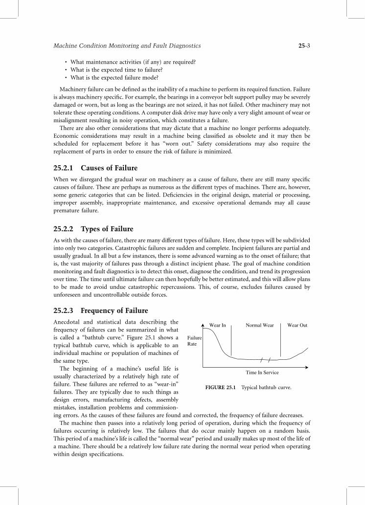
Anecdotal and statistical data describing the

frequency of failures can be summarized in what

is called a “bathtub curve.” Figure 25.1 shows a

typical bathtub curve, which is applicable to an

individual machine or population of machines of

the same type.

The beginning of a machine’s useful life is

usually characterized by a relatively high rate of

failure. These failures are referred to as “wear-in”

failures. They are typically due to such things as

design errors, manufacturing defects, assembly

mistakes, installation problems and commission-

ing errors. As the causes of these failures are found and corrected, the frequency of failure decreases.

The machine then passes into a relatively long period of operation, during which the frequency of

failures occurring is relatively low. The failures that do occur mainly happen on a random basis.

This period of a machine’s life is called the “normal wear” period and usually makes up most of the life of

a machine. There should be a relatively low failure rate during the normal wear period when operating

within design specifications.

FailureRate

Time In Service

Wear In Normal Wear Wear Out

FIGURE 25.1 Typical bathtub curve.

Machine Condition Monitoring and Fault Diagnostics 25-3

As a machine gradually reaches the end of its designed life, the frequency of failures again increases.

These failures are called “wearout” failures. This gradually increasing failure rate at the expected end of a

machine’s useful life is primarily due to metal fatigue, wear mechanisms between moving parts,

corrosion, and obsolescence. The slope of the wearout part of the bathtub curve is machine-dependent.

The rate at which the frequency of failures increases is largely dependent on the design of the machine and

its operational history. If the machine design is such that the operational life ends abruptly, the machine

is underdesigned to meet the load expected, or the machine has endured a severe operational life

(experienced numerous overloads), the slope of the curve in the wearout section will increase sharply

with time. If the machinery is overdesigned or experiences a relatively light loading history, the slope of

this part of the bathtub curve will increase only gradually with time.

25.3 Basic Maintenance Strategies

Maintenance strategies can be divided into three main types: (1) run-to-failure, (2) scheduled, and (3)

condition-based maintenance. Each of these different strategies has distinct advantages and

disadvantages, which will be described below. Specific situations within any large facility may require

the application of a different strategy. Therefore, no one strategy should be considered as always superior

or inferior to another.

25.3.1 Run-to-Failure (Breakdown) Maintenance

Run-to-failure, or breakdown maintenance, is a strategy where maintenance, in the form of repair work

or replacement, is only performed when machinery has failed. In general, run-to-failure maintenance is

appropriate when the following situations exist:

* The equipment is redundant.* Low cost spares are available.* The process is interruptible or there is stockpiled product.* All known failure modes are safe.* There is a known long mean time to failure (MTTF) or a long mean time between failure (MTBF).* There is a low cost associated with secondary damage.* Quick repair or replacement is possible.

An example of the application of run-to-failure maintenance can be found when one considers the

standard household light bulb. This device satisfies all the requirements above and therefore the most

cost-effective maintenance strategy is to replace burnt out light bulbs as needed.

* Generally (outside of start-up and shutdown) machinery is required to operate at constant

speed and load.* Machinery failure is defined based on performance, operating condition, and system

specifications.* Machinery failure can be defined as the inability of a machine to perform its required

function.* Causes of machinery failure can be generally defined as being due to deficiencies in the

original design, material or processing, improper assembly, inappropriate maintenance, or

excessive operation demands.* The frequency of failure for an individual machine or a population of similar machines can

be summarized using a “bathtub curve.”


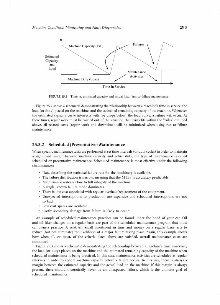
Figure 25.2 shows a schematic demonstrating the relationship between a machine’s time in service, the

load (or duty) placed on the machine, and the estimated remaining capacity of the machine. Whenever

the estimated capacity curve intersects with (or drops below) the load curve, a failure will occur. At

these times, repair work must be carried out. If the situation that exists fits within the “rules” outlined

above, all related costs (repair work and downtime) will be minimized when using run-to-failure

maintenance.

25.3.2 Scheduled (Preventative) Maintenance

When specific maintenance tasks are performed at set time intervals (or duty cycles) in order to maintain

a significant margin between machine capacity and actual duty, the type of maintenance is called

scheduled or preventative maintenance. Scheduled maintenance is most effective under the following

circumstances:

* Data describing the statistical failure rate for the machinery is available.* The failure distribution is narrow, meaning that the MTBF is accurately predictable.* Maintenance restores close to full integrity of the machine.* A single, known failure mode dominates.* There is low cost associated with regular overhaul/replacement of the equipment.* Unexpected interruptions to production are expensive and scheduled interruptions are not

so bad.* Low cost spares are available.* Costly secondary damage from failure is likely to occur.

An example of scheduled maintenance practices can be found under the hood of your car. Oil

and oil filter changes on a regular basis are part of the scheduled maintenance program that most

car owners practice. A relatively small investment in time and money on a regular basis acts to

reduce (but not eliminate) the likelihood of a major failure taking place. Again, this example shows

how when all, or most, of the criteria listed above are satisfied, overall maintenance costs are

minimized.

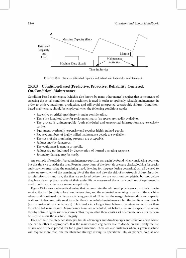
Figure 25.3 shows a schematic demonstrating the relationship between a machine’s time in-service,

the load (or duty) placed on the machine and the estimated remaining capacity of the machine when

scheduled maintenance is being practiced. In this case, maintenance activities are scheduled at regular

intervals in order to restore machine capacity before a failure occurs. In this way, there is always a

margin between the estimated capacity and the actual load on the machine. If this margin is always

present, there should theoretically never be an unexpected failure, which is the ultimate goal of

scheduled maintenance.

Machine Duty (Load)

EstimatedCapacity

andLoad

Time In Service

Machine Capacity (Est.) Failures

MaintenanceActivities

FIGURE 25.2 Time vs. estimated capacity and actual load (run-to-failure maintenance).


25.3.3 Condition-Based (Predictive, Proactive, Reliability Centered,On-Condition) Maintenance

Condition-based maintenance (which is also known by many other names) requires that some means of

assessing the actual condition of the machinery is used in order to optimally schedule maintenance, in

order to achieve maximum production, and still avoid unexpected catastrophic failures. Condition-

based maintenance should be employed when the following conditions apply:

* Expensive or critical machinery is under consideration.* There is a long lead-time for replacement parts (no spares are readily available).* The process is uninterruptible (both scheduled and unexpected interruptions are excessively

costly).* Equipment overhaul is expensive and requires highly trained people.* Reduced numbers of highly skilled maintenance people are available.* The costs of the monitoring program are acceptable.* Failures may be dangerous.* The equipment is remote or mobile.* Failures are not indicated by degeneration of normal operating response.* Secondary damage may be costly.

An example of condition-based maintenance practices can again be found when considering your car,

but this time we consider the tires. Regular inspections of the tires (air pressure checks, looking for cracks

and scratches, measuring the remaining tread, listening for slippage during cornering) can all be used to

make an assessment of the remaining life of the tires and also the risk of catastrophic failure. In order

to minimize costs and risk, the tires are replaced before they are worn out completely, but not before

they have given up the majority of their useful life. A measure of the actual condition of equipment is

used to utilize maintenance resources optimally.

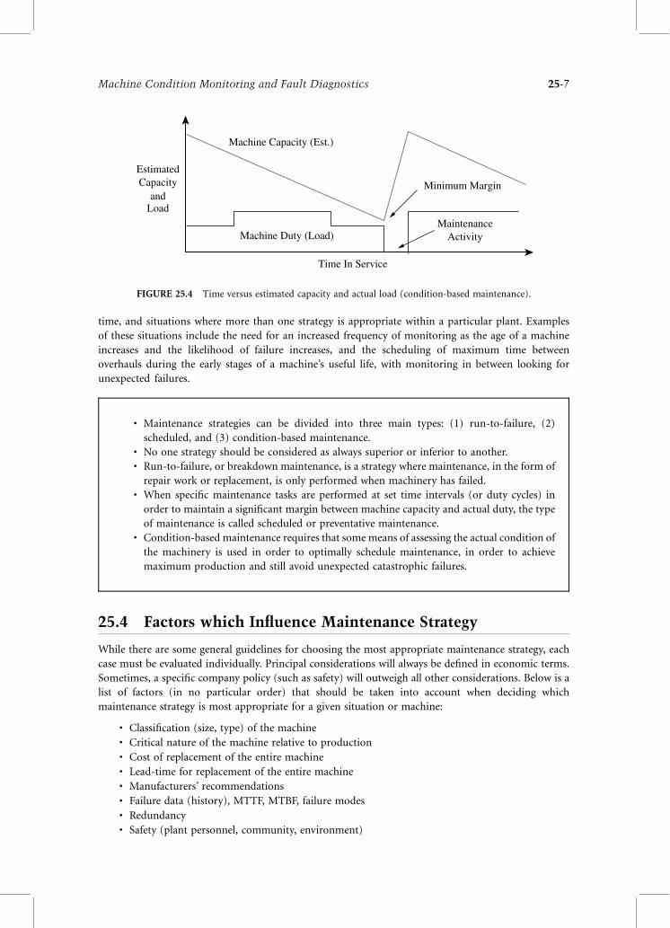
Figure 25.4 shows a schematic drawing that demonstrates the relationship between a machine’s time in

service, the load (or duty) placed on the machine, and the estimated remaining capacity of the machine

when condition-based maintenance is being practiced. Note that the margin between duty and capacity

is allowed to become quite small (smaller than in scheduled maintenance), but the two lines never touch

(as in run-to-failure maintenance). This results in a longer time between maintenance activities than

for scheduled maintenance. Maintenance tasks are scheduled just before a failure is expected to occur,

thereby optimizing the use of resources. This requires that there exists a set of accurate measures that can

be used to assess the machine integrity.

Each of these maintenance strategies has its advantages and disadvantages and situations exist where

one or the other is appropriate. It is the maintenance engineer’s role to decide on and justify the use

of any one of these procedures for a given machine. There are also instances where a given machine

will require more than one maintenance strategy during its operational life, or perhaps even at one

Machine Duty (Load)

EstimatedCapacity

andLoad

Time In Service

Machine Capacity (Est.)

MaintenanceActivities

Margin

FIGURE 25.3 Time vs. estimated capacity and actual load (scheduled maintenance).


time, and situations where more than one strategy is appropriate within a particular plant. Examples

of these situations include the need for an increased frequency of monitoring as the age of a machine

increases and the likelihood of failure increases, and the scheduling of maximum time between

overhauls during the early stages of a machine’s useful life, with monitoring in between looking for

unexpected failures.

25.4 Factors which Influence Maintenance Strategy

While there are some general guidelines for choosing the most appropriate maintenance strategy, each

case must be evaluated individually. Principal considerations will always be defined in economic terms.

Sometimes, a specific company policy (such as safety) will outweigh all other considerations. Below is a

list of factors (in no particular order) that should be taken into account when deciding which

maintenance strategy is most appropriate for a given situation or machine:

* Classification (size, type) of the machine* Critical nature of the machine relative to production* Cost of replacement of the entire machine* Lead-time for replacement of the entire machine* Manufacturers’ recommendations* Failure data (history), MTTF, MTBF, failure modes* Redundancy* Safety (plant personnel, community, environment)

Machine Duty (Load)

EstimatedCapacity

andLoad

Time In Service

Machine Capacity (Est.)

MaintenanceActivity

Minimum Margin

FIGURE 25.4 Time versus estimated capacity and actual load (condition-based maintenance).

* Maintenance strategies can be divided into three main types: (1) run-to-failure, (2)

scheduled, and (3) condition-based maintenance.* No one strategy should be considered as always superior or inferior to another.* Run-to-failure, or breakdown maintenance, is a strategy where maintenance, in the form of

repair work or replacement, is only performed when machinery has failed.* When specific maintenance tasks are performed at set time intervals (or duty cycles) in

order to maintain a significant margin between machine capacity and actual duty, the type

of maintenance is called scheduled or preventative maintenance.* Condition-based maintenance requires that some means of assessing the actual condition of

the machinery is used in order to optimally schedule maintenance, in order to achieve

maximum production and still avoid unexpected catastrophic failures.


* Cost and availability of spare parts* Personnel costs, administrative costs, monitoring equipment costs* Running costs for a monitoring program (if used)

25.5 Machine Condition Monitoring

With the understanding that condition-based maintenance may not be appropriate in all situations, let us

say that some preliminary analysis has been carried out and a decision made to apply machine condition

monitoring and fault diagnostics in a selected part of a plant or on a specific machine. The following is a

list of potential advantages that should be realized:

* Increased machine availability and reliability* Improved operating efficiency* Improved risk management (less downtime)* Reduced maintenance costs (better planning)* Reduced spare parts inventories* Improved safety* Improved knowledge of the machine condition (safe short-term overloading of machine possible)* Extended operational life of the machine* Improved customer relations (less planned/unplanned downtime)* Elimination of chronic failures (root cause analysis and redesign)* Reduction of postoverhaul failures due to improperly performed maintenance or reassembly

There are, of course, also some disadvantages that must be weighed in the decision to use machine

condition monitoring and fault diagnostics. These disadvantages are listed below:

* Monitoring equipment costs (usually significant).* Operational costs (running the program).* Skilled personnel needed.* Strong management commitment needed.* A significant run-in time to collect machine histories and trends is usually needed.* Reduced costs are usually harder to sell to management as benefits when compared with increased

profits.

The ultimate goal of machine condition monitoring and fault diagnostics is to get useful information

on the condition of equipment to the people who need it in a timely manner. The people who need this

information include operators, maintenance engineers and technicians, managers, vendors, and

suppliers. These groups will need different information at different times. The task of the person or

group in charge of condition monitoring and diagnostics must ensure that useful data is collected, that

data is changed into information in a form required by and useful to others, and that the information is

provided to the people who need it when they need it. Further general reading can be found in these

references: Mitchell (1981), Lyon (1987), Mobley (1990), Rao (1996), and Moubray (1997).

The focus of this chapter will be on vibration-based data, but there are several different types of data

that can be useful for assessing machine condition and these should not be ignored. These include

physical parameters related to lubrication analysis (oil/grease quality, contamination), wear particle

monitoring and analysis, force, sound, temperature, output (machine performance), product quality,

odor, and visual inspections. All of these factors may contribute to a complete picture of machine

integrity. The types of information that can be gleaned from the data include existing condition, trends,

expected time to failure at a given load, type of fault existing or developing, and the type of fault that

caused failure.

The specific tasks which must be carried out to complete a successful machine condition

monitoring and fault diagnostics program include detection, diagnosis, prognosis, postmortem, and


prescription. Detection requires data gathering, comparison to standards, comparison to limits set

in-plant for specific equipment, and trending over time. Diagnosis involves recognizing the types of

fault developing (different fault types may be more or less serious and require different action) and

determining the severity of given faults once detected and diagnosed. Prognosis, which is a

very challenging task, involves estimating (forecasting) the expected time to failure, trending the

condition of the equipment being monitored, and planning the appropriate maintenance timing.

Postmortem is the investigation of root-cause failure analysis, and usually involves some research-type

investigation in the laboratory and/or in the field, as well as modeling of the system. Prescription is

an activity that is dictated by the information collected and may be applied at any stage of the

condition monitoring and diagnostic work. It may involve recommendations for altering the

operating conditions, altering the monitoring strategy (frequency, type), or redesigning the process

or equipment.

The tasks listed above have relatively crisp definitions, but there is still considerable room for

adjustment within any condition monitoring and diagnostic program. There are always questions,

concerning such things as how much data to collect and how much time to spend on data analysis,

that need to be considered before the final program is put in place. As mentioned above, things such as

equipment class, size, importance within the process, replacement cost, availability, and safety need

to be carefully considered. Different pieces of equipment or processes may require different monitoring

strategies.

25.5.1 Periodic Monitoring

Periodic monitoring involves intermittent data gathering and analysis with portable, removable

monitoring equipment. On occasion, permanent monitoring hardware may be used for this type of

monitoring strategy, but data is only collected at specific times. This type of monitoring is usually applied

to noncritical equipment where failure modes are well known (historically dependable equipment).

Trending of condition and severity level checks are the main focus, with problems triggering more

rigorous investigations.

25.5.2 Continuous Monitoring

Constant or very frequent data collection and analysis is referred to as continuous monitoring.

Permanently installed monitoring systems are typically used, with samples and analysis of data done

automatically. This type of monitoring is carried out on critical equipment (expensive to replace,

with downtime and lost production also being expensive). Changes in condition trigger more detailed

investigation or possibly an automatic shutdown of the equipment.

* Potential advantages of machine condition monitoring include increased machine

availability and reliability, improved efficiency, reduced costs, extended operational life,

and improved safety.* Some of the disadvantages of condition monitoring include monitoring equipment costs,

operational costs, and training costs.* The ultimate goal of machine condition monitoring and fault diagnostics is to get

useful information on the condition of equipment to the people who need it, in a timely

manner.* The specific tasks which must be carried out to complete a successful machine condition

monitoring and fault diagnostics program include detection, diagnosis, prognosis,

postmortem, and prescription.


25.6 Transducer Selection

A transducer is a device that senses a physical

quantity (vibration in this case, but it can also be

temperature, pressure, etc.) and converts it into an

electrical output signal, which is proportional to

the measured variable (see Chapter 15). As such,

the transducer is a vital link in the measurement

chain. Accurate analysis results depend on an

accurate electrical reproduction of the measured

parameters. If information is missed or distorted

during measurement, it cannot be recovered later.

Hence, the selection, placement, and proper use of

the correct transducer are important steps in the

implementation of a condition monitoring and

fault diagnostics program.

Considerable research and development work has gone into the design, testing, and calibration of

sensors (transducers) for a wide range of applications. The transducer must be:

* Correct for the task* Properly mounted* In good working order (properly calibrated)* Fully understood in terms of operational characteristics

Transducers usually require amplification and conversion electronics to produce a useful output

signal. These circuits may be located within the sealed sensor unit or in a separate box. There are

advantages and disadvantages to both of these configurations but they will not be detailed here.

Traditional vibration sensors fall into three main classes:

* Noncontact displacement transducers (also known as proximity probes or eddy current probes)* Velocity transducers (electro-mechanical, piezoelectric)* Accelerometers (piezoelectric)

Force and frequency considerations dictate the type of measurements and applications that are best

suited for each transducer. Recently, laser-based noncontact velocity/displacement transducers have

become more commonplace. These are still relatively expensive because of their extreme sensitivity, and

hence are still predominantly used in the laboratory setting.

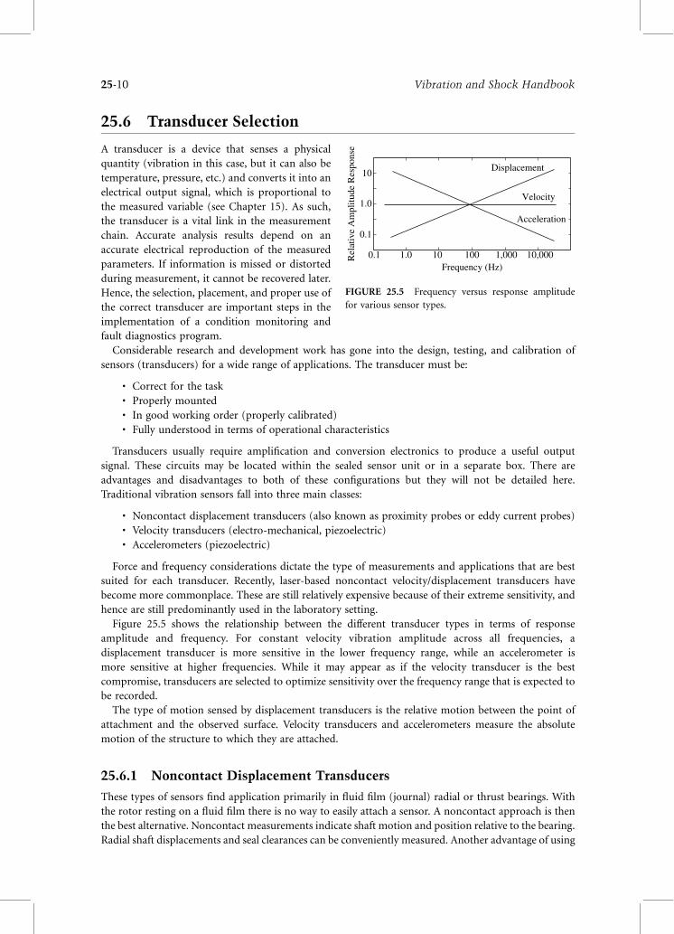
Figure 25.5 shows the relationship between the different transducer types in terms of response

amplitude and frequency. For constant velocity vibration amplitude across all frequencies, a

displacement transducer is more sensitive in the lower frequency range, while an accelerometer is

more sensitive at higher frequencies. While it may appear as if the velocity transducer is the best

compromise, transducers are selected to optimize sensitivity over the frequency range that is expected to

be recorded.

The type of motion sensed by displacement transducers is the relative motion between the point of

attachment and the observed surface. Velocity transducers and accelerometers measure the absolute

motion of the structure to which they are attached.

25.6.1 Noncontact Displacement Transducers

These types of sensors find application primarily in fluid film (journal) radial or thrust bearings. With

the rotor resting on a fluid film there is no way to easily attach a sensor. A noncontact approach is then

the best alternative. Noncontact measurements indicate shaft motion and position relative to the bearing.

Radial shaft displacements and seal clearances can be conveniently measured. Another advantage of using

0.1 1.0 10 100 1,000 10,000

0.1

1.0

10

Rel

ativ

eA

mpl

itude

Res

pons

e

Frequency (Hz)

Velocity

Displacement

Acceleration

FIGURE 25.5 Frequency versus response amplitude

for various sensor types.


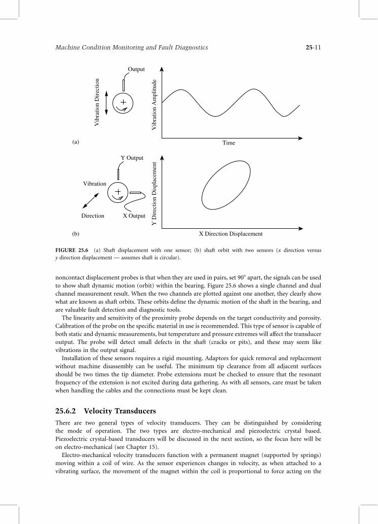
noncontact displacement probes is that when they are used in pairs, set 908 apart, the signals can be used

to show shaft dynamic motion (orbit) within the bearing. Figure 25.6 shows a single channel and dual

channel measurement result. When the two channels are plotted against one another, they clearly show

what are known as shaft orbits. These orbits define the dynamic motion of the shaft in the bearing, and

are valuable fault detection and diagnostic tools.

The linearity and sensitivity of the proximity probe depends on the target conductivity and porosity.

Calibration of the probe on the specific material in use is recommended. This type of sensor is capable of

both static and dynamic measurements, but temperature and pressure extremes will affect the transducer

output. The probe will detect small defects in the shaft (cracks or pits), and these may seem like

vibrations in the output signal.

Installation of these sensors requires a rigid mounting. Adaptors for quick removal and replacement

without machine disassembly can be useful. The minimum tip clearance from all adjacent surfaces

should be two times the tip diameter. Probe extensions must be checked to ensure that the resonant

frequency of the extension is not excited during data gathering. As with all sensors, care must be taken

when handling the cables and the connections must be kept clean.

25.6.2 Velocity Transducers

There are two general types of velocity transducers. They can be distinguished by considering

the mode of operation. The two types are electro-mechanical and piezoelectric crystal based.

Piezoelectric crystal-based transducers will be discussed in the next section, so the focus here will be

on electro-mechanical (see Chapter 15).

Electro-mechanical velocity transducers function with a permanent magnet (supported by springs)

moving within a coil of wire. As the sensor experiences changes in velocity, as when attached to a

vibrating surface, the movement of the magnet within the coil is proportional to force acting on the

(a)

(b)

Vib

ratio

nD

irec

tion

Time

Vib

ratio

nA

mpl

itude

Output

X Direction Displacement

Vibration

YD

irec

tion

Dis

plac

emen

t

Direction

Y Output

X Output

FIGURE 25.6 (a) Shaft displacement with one sensor; (b) shaft orbit with two sensors (x direction versus

y direction displacement — assumes shaft is circular).


sensor. The current in the coil, induced by the

moving magnet, is proportional to velocity, which

in turn is proportional to the force. This type of

device is known as “self-generating” and produces

a low impedance signal; therefore, no additional

signal conditioning is generally needed.

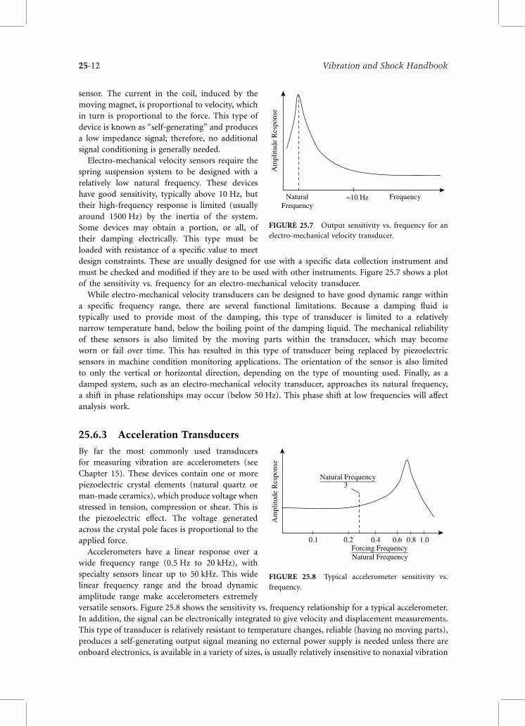
Electro-mechanical velocity sensors require the

spring suspension system to be designed with a

relatively low natural frequency. These devices

have good sensitivity, typically above 10 Hz, but

their high-frequency response is limited (usually

around 1500 Hz) by the inertia of the system.

Some devices may obtain a portion, or all, of

their damping electrically. This type must be

loaded with resistance of a specific value to meet

design constraints. These are usually designed for use with a specific data collection instrument and

must be checked and modified if they are to be used with other instruments. Figure 25.7 shows a plot

of the sensitivity vs. frequency for an electro-mechanical velocity transducer.

While electro-mechanical velocity transducers can be designed to have good dynamic range within

a specific frequency range, there are several functional limitations. Because a damping fluid is

typically used to provide most of the damping, this type of transducer is limited to a relatively

narrow temperature band, below the boiling point of the damping liquid. The mechanical reliability

of these sensors is also limited by the moving parts within the transducer, which may become

worn or fail over time. This has resulted in this type of transducer being replaced by piezoelectric

sensors in machine condition monitoring applications. The orientation of the sensor is also limited

to only the vertical or horizontal direction, depending on the type of mounting used. Finally, as a

damped system, such as an electro-mechanical velocity transducer, approaches its natural frequency,

a shift in phase relationships may occur (below 50 Hz). This phase shift at low frequencies will affect

analysis work.

25.6.3 Acceleration Transducers

By far the most commonly used transducers

for measuring vibration are accelerometers (see

Chapter 15). These devices contain one or more

piezoelectric crystal elements (natural quartz or

man-made ceramics), which produce voltage when

stressed in tension, compression or shear. This is

the piezoelectric effect. The voltage generated

across the crystal pole faces is proportional to the

applied force.

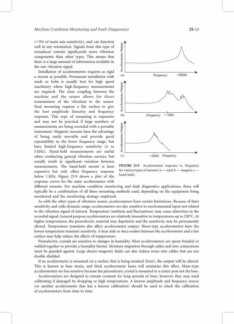
Accelerometers have a linear response over a

wide frequency range (0.5 Hz to 20 kHz), with

specialty sensors linear up to 50 kHz. This wide

linear frequency range and the broad dynamic

amplitude range make accelerometers extremely

versatile sensors. Figure 25.8 shows the sensitivity vs. frequency relationship for a typical accelerometer.

In addition, the signal can be electronically integrated to give velocity and displacement measurements.

This type of transducer is relatively resistant to temperature changes, reliable (having no moving parts),

produces a self-generating output signal meaning no external power supply is needed unless there are

onboard electronics, is available in a variety of sizes, is usually relatively insensitive to nonaxial vibration

AmplitudeResponse

FrequencyNaturalFrequency

≈10 Hz

FIGURE 25.7 Output sensitivity vs. frequency for an

electro-mechanical velocity transducer.

AmplitudeResponse

Forcing FrequencyNatural Frequency

0.1 0.2 0.4 0.6 0.8 1.0

Natural Frequency3

FIGURE 25.8 Typical accelerometer sensitivity vs.

frequency.


(,3% of main axis sensitivity), and can function

well in any orientation. Signals from this type of

transducer contain significantly more vibration

components than other types. This means that

there is a large amount of information available in

the raw vibration signal.

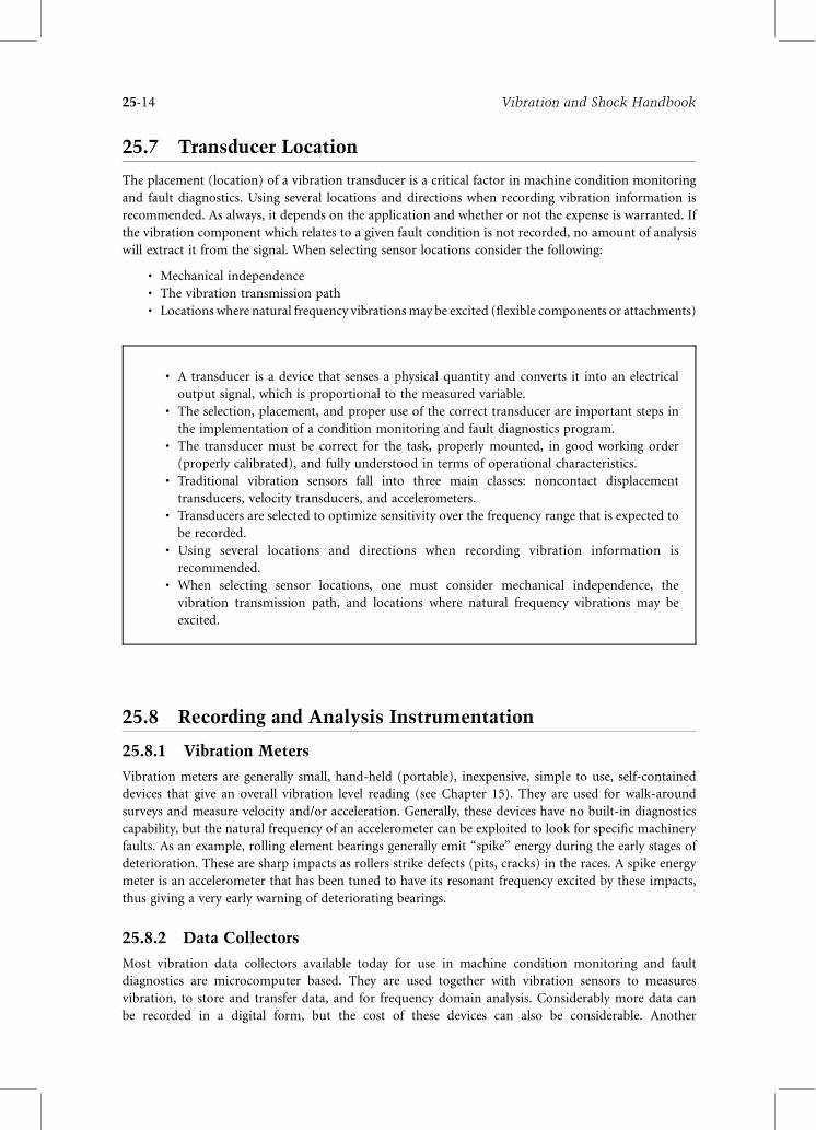
Installation of accelerometers requires as rigid

a mount as possible. Permanent installation with

studs or bolts is usually best for high speed

machinery where high-frequency measurements

are required. The close coupling between the

machine and the sensor allows for direct

transmission of the vibration to the sensor.

Stud mounting requires a flat surface to give

the best amplitude linearity and frequency

response. This type of mounting is expensive

and may not be practical if large numbers of

measurements are being recorded with a portable

instrument. Magnetic mounts have the advantage

of being easily movable and provide good

repeatability in the lower frequency range, but

have limited high-frequency sensitivity (4 to

5 kHz). Hand-held measurements are useful

when conducting general vibration surveys, but

usually result in significant variation between

measurements. The hand-held mount is least

expensive but only offers frequency response

below 1 kHz. Figure 25.9 shows a plot of the

response curves for the same accelerometer with

different mounts. For machine condition monitoring and fault diagnostics applications, there will

typically be a combination of all three mounting methods used, depending on the equipment being

monitored and the monitoring strategy employed.

As with the other types of vibration sensor, accelerometers have certain limitations. Because of their

sensitivity and wide dynamic range, accelerometers are also sensitive to environmental input not related

to the vibration signal of interest. Temperature (ambient and fluctuations) may cause distortion in the

recorded signal. General purpose accelerometers are relatively insensitive to temperatures up to 2508C. At

higher temperatures, the piezoelectric material may depolarize and the sensitivity may be permanently

altered. Temperature transients also affect accelerometer output. Shear-type accelerometers have the

lowest temperature transient sensitivity. A heat sink or mica washer between the accelerometer and a hot

surface may help reduce the effects of temperature.

Piezoelectric crystals are sensitive to changes in humidity. Most accelerometers are epoxy bonded or

welded together to provide a humidity barrier. Moisture migration through cables and into connections

must be guarded against. Large electro-magnetic fields can also induce noise into cables that are not

double shielded.

If an accelerometer is mounted on a surface that is being strained (bent), the output will be altered.

This is known as base strain, and thick accelerometer bases will minimize this effect. Shear-type

accelerometers are less sensitive because the piezoelectric crystal is mounted to a center post not the base.

Accelerometers are designed to remain constant for long periods of time; however, they may need

calibrating if damaged by dropping or high temperatures. A known amplitude and frequency source

(or another accelerometer that has a known calibration) should be used to check the calibration

of accelerometers from time to time.

Frequency

Frequency ≈ 7kHz

Acc

eler

omet

erO

utpu

t

Frequency≈2kHz

Acc

eler

omet

erO

utpu

tA

ccel

erom

eter

Out

put

(a)

(b)

(c)

≈28kHz

FIGURE 25.9 Accelerometer response vs. frequency

for various types of mounts (a— stud; b—magnet; c —

hand held).


25.7 Transducer Location

The placement (location) of a vibration transducer is a critical factor in machine condition monitoring

and fault diagnostics. Using several locations and directions when recording vibration information is

recommended. As always, it depends on the application and whether or not the expense is warranted. If

the vibration component which relates to a given fault condition is not recorded, no amount of analysis

will extract it from the signal. When selecting sensor locations consider the following:

* Mechanical independence* The vibration transmission path* Locations where natural frequency vibrationsmay be excited (flexible components or attachments)

25.8 Recording and Analysis Instrumentation

25.8.1 Vibration Meters

Vibration meters are generally small, hand-held (portable), inexpensive, simple to use, self-contained

devices that give an overall vibration level reading (see Chapter 15). They are used for walk-around

surveys and measure velocity and/or acceleration. Generally, these devices have no built-in diagnostics

capability, but the natural frequency of an accelerometer can be exploited to look for specific machinery

faults. As an example, rolling element bearings generally emit “spike” energy during the early stages of

deterioration. These are sharp impacts as rollers strike defects (pits, cracks) in the races. A spike energy

meter is an accelerometer that has been tuned to have its resonant frequency excited by these impacts,

thus giving a very early warning of deteriorating bearings.

25.8.2 Data Collectors

Most vibration data collectors available today for use in machine condition monitoring and fault

diagnostics are microcomputer based. They are used together with vibration sensors to measures

vibration, to store and transfer data, and for frequency domain analysis. Considerably more data can

be recorded in a digital form, but the cost of these devices can also be considerable. Another

* A transducer is a device that senses a physical quantity and converts it into an electrical

output signal, which is proportional to the measured variable.* The selection, placement, and proper use of the correct transducer are important steps in

the implementation of a condition monitoring and fault diagnostics program.* The transducer must be correct for the task, properly mounted, in good working order

(properly calibrated), and fully understood in terms of operational characteristics.* Traditional vibration sensors fall into three main classes: noncontact displacement

transducers, velocity transducers, and accelerometers.* Transducers are selected to optimize sensitivity over the frequency range that is expected to

be recorded.* Using several locations and directions when recording vibration information is

recommended.* When selecting sensor locations, one must consider mechanical independence, the

vibration transmission path, and locations where natural frequency vibrations may be

excited.


advantage of most data collectors is the ability to use these devices to conduct on-the-spot

diagnostics or balancing. They are usually used with a PC to provide permanent data storage and a

platform for more detailed analysis software. Data collectors are usually used on general-purpose

equipment.

25.8.3 Frequency-Domain Analyzers

The frequency-domain analyzer is perhaps the key instrument for diagnostic work. Different machine

conditions (unbalance, misalignment, looseness, bearing flaws) all generate characteristic patterns that

are usually visible in the frequency domain. While data collectors do provide some frequency domain

analysis capability, their main purpose is data collection. Frequency-domain analyzers are specialized

instruments that emphasize the analysis of vibration signals. As such, they are often treated as a

laboratory instrument. Generally, analyzers will have superior frequency resolution, filtering ability

(including antialiasing), weighting functions for the elimination of leakage, averaging capabilities (both

in the time and frequency domains), envelope detection (demodulation), transient capture, large

memory, order tracking, cascade/waterfall display, and zoom features. Dual-channel analysis is also

common.

25.8.4 Time-Domain Instruments

Time-domain instruments are generally only able to provide a time domain display of the vibration

waveform. Some devices have limited frequency-domain capabilities. While this restriction may seem

limiting, the low cost of these devices and the fact that some vibration characteristics and trends show up

well in the time domain make them valuable tools. Oscilloscopes are the most common form. Shaft

displacements (orbits), transients and synchronous time averaging (and negative averaging) are some of

the analysis strategies that can be employed with this type of device.

25.8.5 Tracking Analyzers

Tracking analyzers are typically used to record and analyze data from machines that are changing speed.

This usually occurs during run-up and coast-down of large machinery or turbo-machinery. These

measurements are typically used to locate machine resonances and unbalance conditions. The tracking

rate is dependent on filter bandwidth, and there is a need for a reference signal to track speed

(tachometer input). These devices usually have variable input sensitivity and a large dynamic range.

* Vibration meters are generally small, hand-held (portable), inexpensive, simple to use, self-

contained devices that give an overall vibration level reading.* Most vibration data collectors available today for use in machine condition monitoring and

fault diagnostics are microcomputer based. They are used together with vibration sensors to

measures vibration, to store and transfer data, and for frequency domain analysis.* Frequency domain analyzers are specialized instruments that emphasize the analysis of

vibration signals, and as such they are perhaps the key instrument for diagnostic work.* Time domain instruments are generally only able to provide a time domain display of the

vibration waveform.* Tracking analyzers are typically used to record and analyze data (locate machine resonances

and unbalance conditions) from machines that are changing speed. This usually occurs

during run-up and coast-down of large machinery or turbo-machinery.


25.9 Display Formats and Analysis Tools

Vibration signals can be displayed in a variety of different formats. Each format has advantages and

disadvantages, but generally the more processing that is done on the dynamic signal, the more specific

information is highlighted and the more extraneous information is discarded. The broad display formats

that will be discussed here are the time domain, the frequency domain, the modal domain, and the

quefrency domain. Within each of these display formats, several different analysis tools (some specific to

that display format) will be described.

25.9.1 Time Domain

The time domain refers to a display or analysis of the vibration data as a function of time. The

principal advantage of this format is that little or no data are lost prior to inspection. This allows for a

great deal of detailed analysis. However, the disadvantage is that there is often too much data for easy

and clear fault diagnosis. Time-domain analysis of vibration signals can be subdivided into the

following sections.

25.9.1.1 Time-Waveform Analysis

Time-waveform analysis involves the visual inspection of the time-history of the vibration signal. The

general nature of the vibration signal can be clearly seen and distinctions made between sinusoidal,

random, repetitive, and transient events. Nonsteady-state conditions, such as run-up and coast-down,

are most easily captured and analyzed using time waveforms. High-speed sampling can reveal such

defects as broken gear teeth and cracked bearing races, but can also result in extremely large amounts of

data being collected — much of which is likely to be redundant and of little use.

25.9.1.2 Time-Waveform Indices

A time-waveform index is a single number calculated in some way based on the raw vibration signal and

used for trending and comparisons. These indices significantly reduce the amount of data that is

presented for inspection, but highlight differences between samples. Examples of time-waveform-based

indices include the peak level (maximum vibration amplitude within a given time signal), mean level

(average vibration amplitude), root-mean-square (RMS) level (peak level=ffiffi2

p; reduces the effect of

spurious peaks caused by noise or transient events), and peak-to-peak amplitude (maximum positive to

maximum negative signal amplitudes). All of these measures are affected adversely when more than one

machinery component contributes to the measured signal. The crest factor is the ratio of the peak level to

the RMS level ðpeak level=RMS levelÞ; and indicates the early stages of rolling-element-bearing failure.However, the crest factor decreases with progressive failure because the RMS level generally increases with

progressive failure.

25.9.1.3 Time-Synchronous Averaging

Averaging of the vibration signal synchronous with the running speed of the machinery being monitored

is called time-synchronous averaging. When taken over many machine cycles, this technique removes

background noise and nonsynchronous events (random transients) from the vibration signal. This

technique is extremely useful where multiple shafts that are operating at only slightly different speeds and

in close proximity to one another are being monitored. A reference signal (usually from a tachometer) is

always needed.

25.9.1.4 Negative Averaging

Negative averaging works in the opposite way to time-synchronous averaging. Rather than averaging all

the collected data, a baseline signal is recorded and then subtracted from all subsequent signals to reveal

changes and transients only. This type of signal processing is useful on equipment or components that are

isolated from other sources of vibrations.


25.9.1.5 Orbits

As described above, orbits are plots of the X direction displacement vs. the Y direction displacement

(phase shifted by 908). This display format shows journal bearing relative motion (bearing wear, shaft

misalignment, shaft unbalance, lubrication instabilities [whirl, whip], and seal rubs) extremely well, and

hence is a powerful monitoring and diagnostic tool, especially on relatively low-speed machinery.

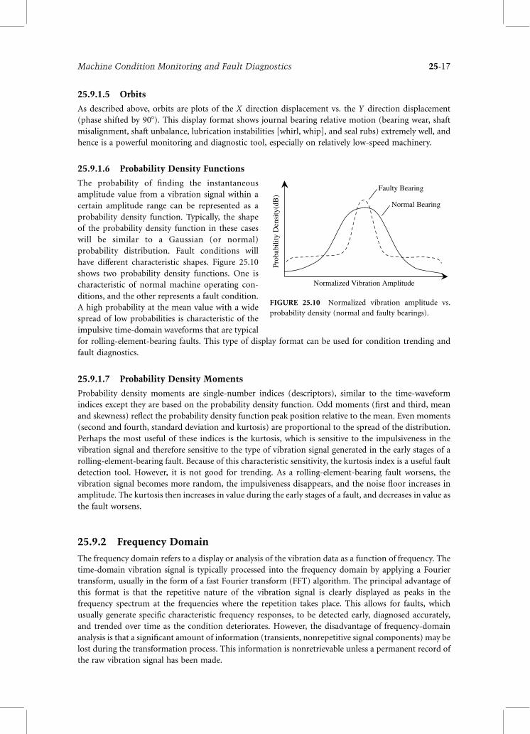
25.9.1.6 Probability Density Functions

The probability of finding the instantaneous

amplitude value from a vibration signal within a

certain amplitude range can be represented as a

probability density function. Typically, the shape

of the probability density function in these cases

will be similar to a Gaussian (or normal)

probability distribution. Fault conditions will

have different characteristic shapes. Figure 25.10

shows two probability density functions. One is

characteristic of normal machine operating con-

ditions, and the other represents a fault condition.

A high probability at the mean value with a wide

spread of low probabilities is characteristic of the

impulsive time-domain waveforms that are typical

for rolling-element-bearing faults. This type of display format can be used for condition trending and

fault diagnostics.

25.9.1.7 Probability Density Moments

Probability density moments are single-number indices (descriptors), similar to the time-waveform

indices except they are based on the probability density function. Odd moments (first and third, mean

and skewness) reflect the probability density function peak position relative to the mean. Even moments

(second and fourth, standard deviation and kurtosis) are proportional to the spread of the distribution.

Perhaps the most useful of these indices is the kurtosis, which is sensitive to the impulsiveness in the

vibration signal and therefore sensitive to the type of vibration signal generated in the early stages of a

rolling-element-bearing fault. Because of this characteristic sensitivity, the kurtosis index is a useful fault

detection tool. However, it is not good for trending. As a rolling-element-bearing fault worsens, the

vibration signal becomes more random, the impulsiveness disappears, and the noise floor increases in

amplitude. The kurtosis then increases in value during the early stages of a fault, and decreases in value as

the fault worsens.

25.9.2 Frequency Domain

The frequency domain refers to a display or analysis of the vibration data as a function of frequency. The

time-domain vibration signal is typically processed into the frequency domain by applying a Fourier

transform, usually in the form of a fast Fourier transform (FFT) algorithm. The principal advantage of

this format is that the repetitive nature of the vibration signal is clearly displayed as peaks in the

frequency spectrum at the frequencies where the repetition takes place. This allows for faults, which

usually generate specific characteristic frequency responses, to be detected early, diagnosed accurately,

and trended over time as the condition deteriorates. However, the disadvantage of frequency-domain

analysis is that a significant amount of information (transients, nonrepetitive signal components) may be

lost during the transformation process. This information is nonretrievable unless a permanent record of

the raw vibration signal has been made.

ProbabilityDensity(dB)

Normalized Vibration Amplitude

Normal Bearing

Faulty Bearing

FIGURE 25.10 Normalized vibration amplitude vs.

probability density (normal and faulty bearings).


25.9.2.1 Band-Pass Analysis

Band-pass analysis is perhaps the most basic of all frequency-domain analysis techniques, and involves

filtering the vibration signal above and/or below specific frequencies in order to reduce the amount of

information presented in the spectrum to a set band of frequencies. These frequencies are typically where

fault characteristic responses are anticipated. Changes in the vibration signal outside the frequency band

of interest are not displayed.

25.9.2.2 Shock Pulse (Spike Energy)

The shock-pulse index (also known as spike energy; Boto, 1979) is derived when an accelerometer is

tuned such that the resonant frequency of the device is close to the characteristic responses frequency

caused by a specific type of machine fault. Typically, accelerometers are designed so that their natural

frequency is significantly above the expected response signals that will be measured. If higher

frequencies are expected, they are filtered out of the vibration signal. High-speed rolling-

element bearings that are experiencing the earlier stages of failure (pitting on interacting surfaces)

emit vibration energy in a relatively high, but closely defined, frequency band. An accelerometer

that is tuned to 32 kHz will be a sensitive detection device. This type of device is simple, effective,

and inexpensive tool for fault detection in high-speed rolling-element bearings. The response from

this type of device is load-dependent and may be prone to false alarms if measurement conditions are

not constant.

25.9.2.3 Enveloped Spectrum

Another powerful analysis tool that is available in the frequency domain and can be effectively applied to

detecting and diagnosing rolling-element-bearing faults is the enveloped spectrum (Courrech, 1985).

When the vibration signal time waveform is demodulated (high-pass filtered, rectified, then low-pass

filtered) the frequency spectrum that results is said to be enveloped. This process effectively filters out

the impulsive components in signals that have high noise levels and other strong transient signal

components, leaving only the components that are related to the bearing characteristic defect

frequencies. This method of analysis is useful for detecting bearing damage in complex machinery where

the vibration signal may be contaminated by signals from other sources. However, the filtering bands

must be chosen with good judgment. Recall also, the impulsive nature of the fault signal at the

characteristic defect frequency leaves as the fault deteriorates.

25.9.2.4 Signature Spectrum

The signature spectrum (Braun, 1986) is a baseline frequency spectrum taken from new or recently

overhauled machinery. It is then later compared with spectra taken from the same machinery that

represent current conditions. The unique nature of each machine and installation is automatically taken

into account. Characteristic component and fault frequencies can be clearly seen and comparisons made

manually (by eye), using indices, or using automated pattern recognition techniques.

25.9.2.5 Cascades (Waterfall Plots)

Cascade plots (also known as waterfall plots) are successive spectra plotted with respect to time and

displayed in a three-dimensional manner. Changing trends can be seen easily, which makes this type of

display a useful fault detection and trending tool. This type of display is also used when a transient event,

such as a coast-down, is known to be about to occur. Cascade plots can also be linked to the speed of a

machine. In this case, the horizontal axis is labeled in multiples of the rotational speed of the machine.

Each multiple of the rotational speed is referred to as an “order.”

“Order tracking” is the name commonly used to refer to cascade plots that are synchronously linked to

the machine rotational speed via a tachometer. As the speed of the machine changes, the responses at

specific frequencies change relative to the speed, but are still tracked in each time-stamped spectra by the

changing horizontal axis scale.


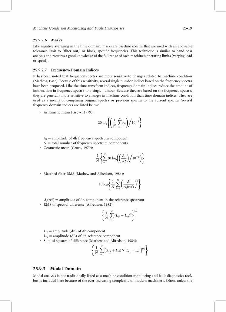
25.9.2.6 Masks

Like negative averaging in the time domain, masks are baseline spectra that are used with an allowable

tolerance limit to “filter out,” or block, specific frequencies. This technique is similar to band-pass

analysis and requires a good knowledge of the full range of each machine’s operating limits (varying load

or speed).

25.9.2.7 Frequency-Domain Indices

It has been noted that frequency spectra are more sensitive to changes related to machine condition

(Mathew, 1987). Because of this sensitivity, several single number indices based on the frequency spectra

have been proposed. Like the time-waveform indices, frequency-domain indices reduce the amount of

information in frequency spectra to a single number. Because they are based on the frequency spectra,

they are generally more sensitive to changes in machine condition than time domain indices. They are

used as a means of comparing original spectra or previous spectra to the current spectra. Several

frequency domain indices are listed below:

* Arithmetic mean (Grove, 1979):

20 log1

N

XNi¼1

Ai

!1025

( )

Ai ¼ amplitude of ith frequency spectrum component

N ¼ total number of frequency spectrum components* Geometric mean (Grove, 1979):

1

N

XNi¼1

20 logAiffiffi2

p 1025( )

* Matched filter RMS (Mathew and Alfredson, 1984):

10 log1

N

XNi¼1

Ai

Aiðref Þ2

( )

Aiðref Þ ¼ amplitude of ith component in the reference spectrum* RMS of spectral difference (Alfredson, 1982):

1

N

XNi¼1

ðLci 2 LoiÞ2( )1=2

Lci ¼ amplitude (dB) of ith component

Loi ¼ amplitude (dB) of ith reference component* Sum of squares of difference (Mathew and Alfredson, 1984):

1

N

XNi¼1

ðLci þ LoiÞ £ lLci 2 Loil1=2

( )

25.9.3 Modal Domain

Modal analysis is not traditionally listed as a machine condition monitoring and fault diagnostics tool,

but is included here because of the ever-increasing complexity of modern machinery. Often, unless the


natural (free and forced response) frequencies of machinery, their support structure, and the

surrounding buildings are fully understood, a complete and accurate assessment of existing

machinery condition is not possible. A complete overview of modal analysis will not be provided

here, but a specific approach to modal analysis (operational deflection shape [ODS] analysis) will

be described.

ODS analysis is like other types of modal analysis in that a force input is provided to a structure or

machine and then the response is measured. The response at different frequencies defines the natural

frequencies of the structure or machine. Typically, an impact or constant frequency force is used to

excite the structure. In the case of ODSs, the regular operation of the machinery provides the

excitation input. With vibration sensors placed at critical locations and a reference signal linking

together all the recorded signals, a simple animation showing how the machine or structure deflects

under normal operation can be generated. These animations, along with the frequency information

contained in each individual signal, can provide significant insights into how a machine or structure

deforms under a dynamic load. This information, in turn, can be a useful addition to other data when

attempting to diagnose problems.

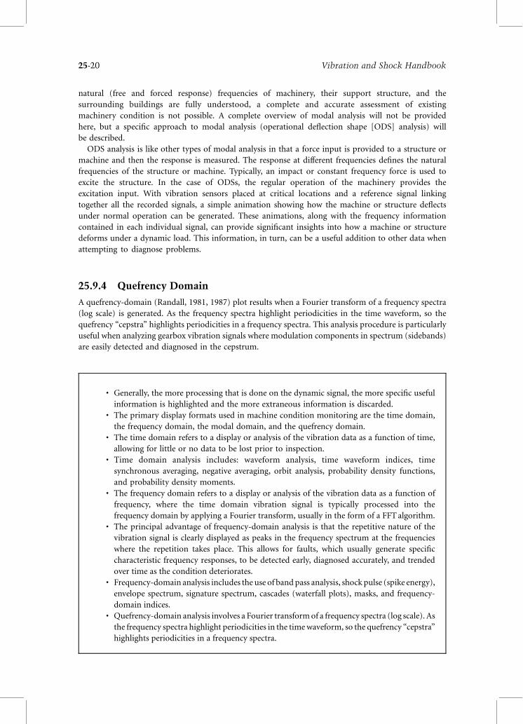
25.9.4 Quefrency Domain

A quefrency-domain (Randall, 1981, 1987) plot results when a Fourier transform of a frequency spectra

(log scale) is generated. As the frequency spectra highlight periodicities in the time waveform, so the

quefrency “cepstra” highlights periodicities in a frequency spectra. This analysis procedure is particularly

useful when analyzing gearbox vibration signals where modulation components in spectrum (sidebands)

are easily detected and diagnosed in the cepstrum.

* Generally, the more processing that is done on the dynamic signal, the more specific useful

information is highlighted and the more extraneous information is discarded.* The primary display formats used in machine condition monitoring are the time domain,

the frequency domain, the modal domain, and the quefrency domain.* The time domain refers to a display or analysis of the vibration data as a function of time,

allowing for little or no data to be lost prior to inspection.* Time domain analysis includes: waveform analysis, time waveform indices, time

synchronous averaging, negative averaging, orbit analysis, probability density functions,

and probability density moments.* The frequency domain refers to a display or analysis of the vibration data as a function of

frequency, where the time domain vibration signal is typically processed into the

frequency domain by applying a Fourier transform, usually in the form of a FFT algorithm.* The principal advantage of frequency-domain analysis is that the repetitive nature of the

vibration signal is clearly displayed as peaks in the frequency spectrum at the frequencies

where the repetition takes place. This allows for faults, which usually generate specific

characteristic frequency responses, to be detected early, diagnosed accurately, and trended

over time as the condition deteriorates.* Frequency-domain analysis includes the use of bandpass analysis, shock pulse (spike energy),

envelope spectrum, signature spectrum, cascades (waterfall plots), masks, and frequency-

domain indices.* Quefrency-domain analysis involves a Fourier transformof a frequency spectra (log scale). As

the frequency spectra highlight periodicities in the timewaveform, so the quefrency “cepstra”

highlights periodicities in a frequency spectra.


25.10 Fault Detection

In many discussions of machine condition monitoring and fault diagnostics, the distinction between

fault detection and fault diagnosis is not made. Here, they have been divided into separate sections in

order to highlight the differences and clarify why they should be treated as separate tasks. Fault detection

can be defined as the departure of a measurement parameter from a range that is known to represent

normal operation. Such a departure then signals the existence of a faulty condition. Given that

measurement parameters are being recorded, what is needed for fault detection is a definition of an

acceptable range for the measurement parameters to fall within. There are two methods for setting

suitable ranges: (1) comparison of recorded signals to known standards and (2) comparison of the

recorded signals to acceptance limits.

25.10.1 Standards

One of the best known sources of standards is the International Organization for Standardization

(ISO). These standards are technology oriented and are set by teams of international experts. ISO

Technical Committee 108, Sub-Committee 5 is responsible for standards for condition monitoring

and diagnostics of machines. This group is further divided into a number of working groups who

review data and draft preliminary standards. Each working group has a particular focus such as

terminology, data interpretation, performance monitoring, or tribology-based machine condition

monitoring.

While ISO is perhaps the most widely known standardization organization, there are several others

that are focused on specific industries. Examples of these include the International Electrical

Commission, which is primarily product oriented, and the American National Standards Institute

(ANSI), which is a nongovernment agency. There are also different domestic government agencies

that vary from country to country. National defense departments also tend to set their own

standards.

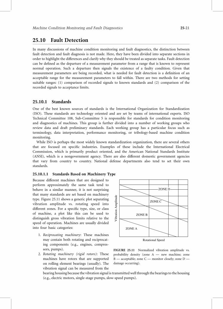
25.10.1.1 Standards Based on Machinery Type

Because different machines that are designed to

perform approximately the same task tend to

behave in a similar manner, it is not surprising

that many standards are set based on machinery

type. Figure 25.11 shows a generic plot separating

vibration amplitude vs. rotating speed into

different zones. For a specific type, size, or class

of machine, a plot like this can be used to

distinguish gross vibration limits relative to the

speed of operation. Machines are usually divided

into four basic categories:

1. Reciprocating machinery: These machines

may contain both rotating and reciprocat-

ing components (e.g., engines, compres-

sors, pumps).

2. Rotating machinery (rigid rotors): These

machines have rotors that are supported

on rolling element bearings (usually). The

vibration signal can be measured from the

bearing housing because the vibration signal is transmittedwell through the bearings to the housing

(e.g., electric motors, single-stage pumps, slow-speed pumps).

VibrationAmplitude

Rotational Speed

ZONE A

ZONE B

ZONE C

ZONE D

FIGURE 25.11 Normalized vibration amplitude vs.

probability density (zone A — new machine; zone

B — acceptable; zone C — monitor closely; zone D —

damage occurring).


3. Rotatingmachinery (flexible rotors): Thesemachines have rotors that are supported on journal (fluid

film) bearings. The movement of the rotor must be measured using proximity probes (e.g., large

steam turbines, multistage pumps, compressors). These machines are subject to critical speeds

(high vibration levels when the speed of rotation excites a natural frequency). Different modes of

vibration may occur at different speeds.

4. Rotating machinery (quasi-rigid rotors): These are usually specialty machines in which some

vibration gets through the bearings, but it is not always trustworthy data (e.g., low-pressure steam

turbines, axial flow compressors, fans).

25.10.1.2 Standards Based on Vibration Severity

It is an oversimplification to say that vibration levels must always be kept low. Standards depend on

many things, including the speed of the machinery, the type and size of the machine, the service

(load) expected, the mounting system, and the effect of machinery vibration on the surrounding

environment. Standards that are based on vibration severity can be divided into two basic

categories:

1. Small-to-medium sized machines: These machines usually operate with shaft speeds of between 600

and 12,000 rpm. The highest broadband RMS value usually occurs in the frequency range of 10 to

1000 Hz.

2. Large machines: These machines usually operate with shaft speeds of 600 to 1200 rpm. If the

machine is rigidly supported, the machine’s fundamental resonant frequency will be above the

main excitation frequency. If the machine is mounted on a flexible support, the machine’s

fundamental resonant frequency will be below the main excitation frequency.

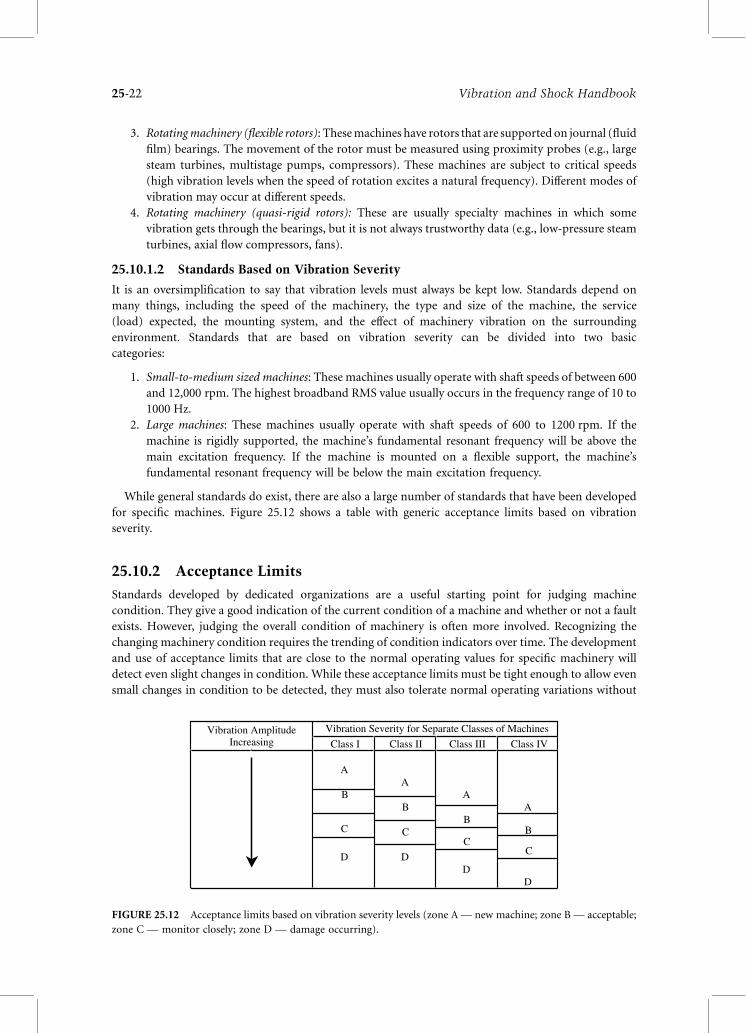
While general standards do exist, there are also a large number of standards that have been developed

for specific machines. Figure 25.12 shows a table with generic acceptance limits based on vibration

severity.

25.10.2 Acceptance Limits

Standards developed by dedicated organizations are a useful starting point for judging machine

condition. They give a good indication of the current condition of a machine and whether or not a fault

exists. However, judging the overall condition of machinery is often more involved. Recognizing the

changing machinery condition requires the trending of condition indicators over time. The development

and use of acceptance limits that are close to the normal operating values for specific machinery will

detect even slight changes in condition. While these acceptance limits must be tight enough to allow even

small changes in condition to be detected, they must also tolerate normal operating variations without

Vibration AmplitudeIncreasing

Vibration Severity for Separate Classes of Machines

Class I Class II Class III Class IV

A

B

C

D

A

B

C

D

A

B

C

D

A

B

C

D

FIGURE 25.12 Acceptance limits based on vibration severity levels (zone A— new machine; zone B — acceptable;

zone C — monitor closely; zone D — damage occurring).


generating false alarms. There are two types of limits:

1. Absolute limits represent conditions that could result in catastrophic failure. These limits are

usually physical constraints such as the allowable movement of a rotating part before contact is

made with stationary parts.

2. Change limits are essentially warning levels that provide warning well in advance of the absolute

limit. These vibration limits are set based on standards and experience with a particular class of

machinery or a particular machine. Change limits are usually based on overall vibration levels.

It is important to note that the early discovery of faulty conditions is a key to optimizing

maintenance effort by allowing the longest possible lead-time for decision making. As well as the overall

vibration levels being monitored, the rates of change are also important. The rate of change of a

vibration level will often provide a strong indication of the expected time until absolute limits

are exceeded. In general, relatively high but stable vibration levels are of less concern than relatively low

but rapidly increasing levels.

An example of how acceptance limits may be used to detect faults and trend condition is provided

when the gradual deterioration of rolling-element bearings is considered. Rolling-element bearings

generate distinctive defect characteristic frequencies in the frequency spectrum during a slow,

progressive failure. Vibration levels can be monitored to achieve maximum useful life and failure

avoidance. Typically, the vibration levels increase as a fault is initiated in the early stages of

deterioration, but then decrease in the later stages as the deterioration becomes more advanced.

Appropriately, set acceptance levels will detect the early onset of the fault and allow subsequent

monitoring to take place even after the overall vibration level has dropped. However, rapid bearing

deterioration may still occur due to a sudden loss of lubrication, lubrication contamination, or a

sudden overload. The possibility of these situations emphasizes the need for carefully selected

acceptance limits.

It should also be noted that changes in operating conditions, such as speed or load changes, could

invalidate time trends. Comparisons must take this into consideration.

25.10.2.1 Statistical Limits

Statistical acceptance limits are set using statistical information calculated from the vibration signals

measured from the equipment that the limits will ultimately be used with. As many vibration signals as

possible are recorded, and the average of the overall vibration level is calculated. An alert or warning

level can then be set at 2.5 standard deviations above or below the average reading (Mechefske, 1998).

This level has been found to provide optimum sensitivity to small changes in machine condition and

maximum immunity to false alarms. A distinct advantage to using this method to set alarm levels is the

fact that the settings are based on actual conditions being experienced by the machine that is being

monitored. This process accommodates normal variations that exist between machines and takes into

account the initial condition of the machine.

25.10.3 Frequency-Domain Limits

Judging vibration characteristics within the frequency spectra is sometimes a more accurate method of

detecting and trending fault conditions. It can also provide earlier detection of specific faults because,

as mentioned previously, the frequency domain is generally more sensitive to changes in the vibration

signal that result from changes in machine condition. The different specific methods are listed and

described below.

25.10.3.1 Limited Band Monitoring

In limited band monitoring, the frequency spectrum is divided into frequency bands. The total energy

or highest amplitude frequency is then trended within each band. Each band has its own limits based

on experience. Generally, ten or fewer bands are used. Small changes in component-specific frequency


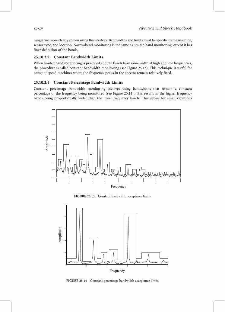
ranges are more clearly shown using this strategy. Bandwidths and limits must be specific to the machine,

sensor type, and location. Narrowband monitoring is the same as limited band monitoring, except it has

finer definition of the bands.

25.10.3.2 Constant Bandwidth Limits

When limited band monitoring is practiced and the bands have same width at high and low frequencies,

the procedure is called constant bandwidth monitoring (see Figure 25.13). This technique is useful for

constant speed machines where the frequency peaks in the spectra remain relatively fixed.

25.10.3.3 Constant Percentage Bandwidth Limits

Constant percentage bandwidth monitoring involves using bandwidths that remain a constant

percentage of the frequency being monitored (see Figure 25.14). This results in the higher frequency

bands being proportionally wider than the lower frequency bands. This allows for small variations

Frequency

Am

plit

ude

FIGURE 25.13 Constant bandwidth acceptance limits.

Frequency

Am

plitu

de

FIGURE 25.14 Constant percentage bandwidth acceptance limits.


in speed without the frequency peaks moving between bands, which may have different

acceptance limits.

25.11 Fault Diagnostics

Depending on the type of equipment being monitored and the maintenance strategy being followed,

once a faulty condition has been detected and the severity of the fault assessed, repair work or

replacement will be scheduled. However, in many situations, the maintenance strategy involves further

analysis of the vibration signal to determine the actual type of fault present. This information then allows

for a more accurate estimation of the remaining life, the replacement parts that are needed, and the

maintenance tools, personnel, and time required to repair the machinery. For these reasons, and many

more, it is often advantageous to have some idea of the fault type that exists before decisions regarding

maintenance actions are made.

There are obviously a large number of potential different fault types. The description of these faults can

be systemized somewhat by considering the type of characteristic defect frequencies generated

(synchronous to rotating speed, subsynchronous, harmonics related to rotating speed, nonsynchronous

harmonics, etc.). Such a systemization requires a focus on frequency-domain analysis tools (primarily

frequency spectra). While this organization strategy is effective, it inherently leaves out potentially

valuable information from other display formats. For this reason, the various faults that usually develop

in machinery are listed here in terms of the forcing functions that cause them and specific machine types.

In this way, a diagnostic template can be developed for the different types of faults that are common in a

given facility or plant. Further reading on machinery diagnostics can be found in these references:

Wowk (1991), Taylor (1994), Eisenmann and Eisenmann (1998), Goldman (1999), and Reeves (1999).

25.11.1 Forcing Functions

Listed and described below are a variety of forcing functions that can result in accelerated deterioration of

machinery or are the result of damaged or worn mechanical components. The list is not meant to be

exhaustive and is in no particular order.

* Fault detection can be defined as the departure of a measurement parameter from a range

that is known to represent normal operation. Such a departure signals the existence of a

faulty condition.* ISO Technical Committee 108, Sub-Committee 5 is responsible for standards for Condition

Monitoring and Diagnostics of Machines.* Standards are based on machinery type or vibration severity.* The development and use of acceptance limits that are close to normal operating values for

specific machinery will detect even slight changes in condition.* Statistical acceptance limits are set using statistical information calculated from

the vibration signals measured from the equipment that the limits will ultimately be

used with.* Judging vibration characteristics within the frequency spectra is sometimes a more accurate

method of the early detecting and trending of fault conditions because the frequency

domain is generally more sensitive to changes in the vibration signal that result from

changes in machine condition.* Frequency domain limits include limited band monitoring, constant bandwidth limits, and

constant percentage bandwidth limits.


25.11.1.1 Unbalance

Unbalance (also referred to as imbalance) exists when the center of mass of a rotating component is not

coincident with the center of rotation. It is practically impossible to fabricate a component that is

perfectly balanced; hence, unbalance is a relatively common condition in a rotor or other rotating

component (flywheel, fan, gear, etc.). The degree to which an unbalance affects the operation of

machinery dictates whether or not it is a problem.

The causes of unbalance include excess mass on one side of the rotor, low tolerances during fabrication

(casting, machining, assembly), variation within materials (voids, porosity, inclusions, etc.), nonsym-

metry of design, aerodynamic forces, and temperature changes. The vector sum of all the different sources

of unbalance can be combined into a single vector. This vector then represents an imaginary heavy spot

on the rotor. If this heavy spot can be located and the unbalance force quantified, then placing an

appropriate weight 1808 from the heavy spot will counteract the original unbalance. If left uncorrected,

unbalance can result in excessive bearing wear, fatigue in support structures, decreased product quality,

power losses, and disturbed adjacent machinery.

Unbalance results in a periodic vibration signal with the same amplitude each shaft rotation (3608).

A strong radial vibration at the fundamental frequency, 1X, (1 £ rotational speed) is the characteristic

diagnostic symptom. If the rotor is overhung, there will also be a strong axial vibration at 1X. The

amplitude of the response is related to the square of the rotational speed, making unbalance a

dangerous condition in machinery that runs at high rotational speeds. In variable speed machines

(or machines that must be run-up to speed gradually), the effects of unbalance will vary with the shaft

rotational speed. At low speeds, the high spot (location of maximum displacement of the shaft) will be

at the same location as the unbalance. At increased speeds, the high spot will lag behind the unbalance

location. At the shaft first critical speed (the first resonance), the lag reaches 908, and at the second

critical and above, the lag reaches 1808.

A special form of unbalance is caused by a bent shaft or bowed rotor. These two conditions are

essentially the same; only the location distinguishes them. A bent shaft is located outside the machine

housing, while a bowed rotor is inside the machine housing. This condition is seen on large machines

(with heavy rotors) that have been allowed to sit idle for a long time. Gravity and time cause the natural

sag in the rotor to become permanent.

The vibration spectrum from a machine with a bent shaft or bowed rotor is identical to

unbalance, largely because it is an unbalanced condition. Bent shafts and bowed rotors are difficult

to correct (straighten), so they need to be balanced by adding counterweights as described above.

The best way to avoid this condition is to keep the shaft/rotor rotating slowly when the machine is

not in use.

25.11.1.2 Misalignment

While misalignment can occur in several different places (between shafts and bearings, between gears,

etc.), the most common form is when two machines are coupled together. In this case, there are two

main categories of misalignment: (1) parallel misalignment (also known as offset) and (2) angular

misalignment. Parallel misalignment occurs when shaft centerlines are parallel but offset from one

another in the horizontal or vertical direction, or a combination of both. Angular misalignment

occurs when the shaft centerlines meet at an angle. The intersection may be at the driver or driven end,

between the coupled units or behind one of the coupled units. Most misalignment is a combination of

these two types.

Misalignment is another major cause of excessive machinery vibration. It is usually caused

by improper machine installation. Flexible couplings can tolerate some shaft misalignment, but

misalignment should always be minimized.

The vibration caused by misalignment results in excessive radial loads on bearings, which in turn

causes premature bearing failure. Elevated 1X vibrations with harmonics (usually up to the third, but

sometimes up to the sixth) in the frequency spectrum are the usual diagnostic signatures. The harmonics


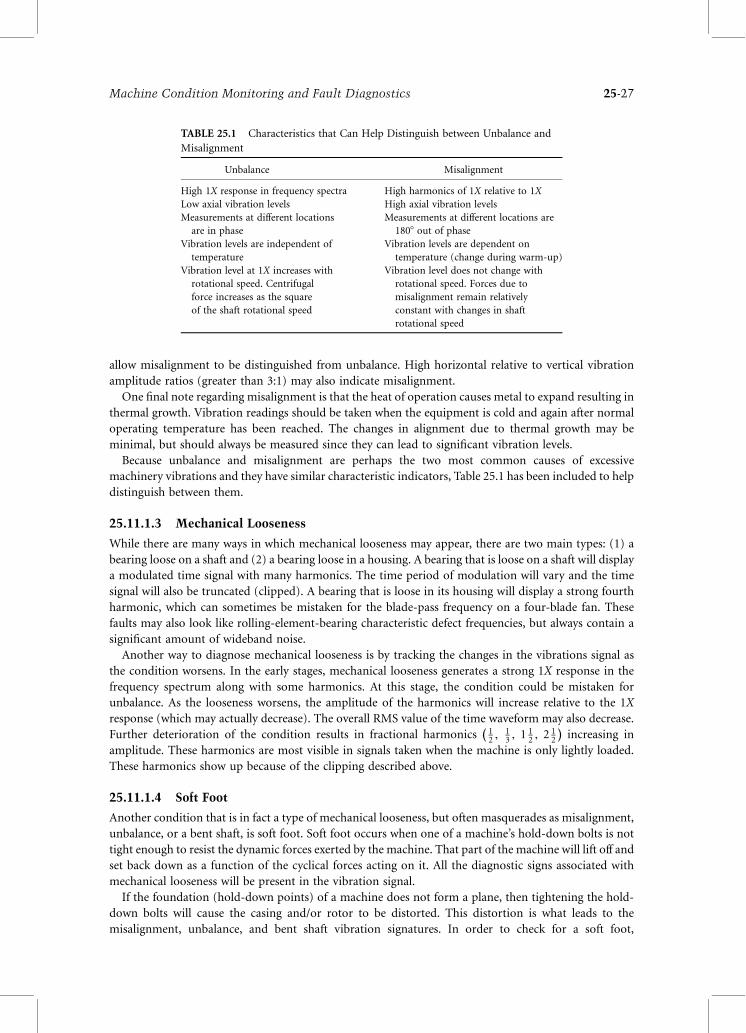
allow misalignment to be distinguished from unbalance. High horizontal relative to vertical vibration

amplitude ratios (greater than 3:1) may also indicate misalignment.

One final note regarding misalignment is that the heat of operation causes metal to expand resulting in

thermal growth. Vibration readings should be taken when the equipment is cold and again after normal

operating temperature has been reached. The changes in alignment due to thermal growth may be

minimal, but should always be measured since they can lead to significant vibration levels.

Because unbalance and misalignment are perhaps the two most common causes of excessive

machinery vibrations and they have similar characteristic indicators, Table 25.1 has been included to help

distinguish between them.

25.11.1.3 Mechanical Looseness

While there are many ways in which mechanical looseness may appear, there are two main types: (1) a

bearing loose on a shaft and (2) a bearing loose in a housing. A bearing that is loose on a shaft will display

a modulated time signal with many harmonics. The time period of modulation will vary and the time

signal will also be truncated (clipped). A bearing that is loose in its housing will display a strong fourth

harmonic, which can sometimes be mistaken for the blade-pass frequency on a four-blade fan. These

faults may also look like rolling-element-bearing characteristic defect frequencies, but always contain a

significant amount of wideband noise.

Another way to diagnose mechanical looseness is by tracking the changes in the vibrations signal as

the condition worsens. In the early stages, mechanical looseness generates a strong 1X response in the

frequency spectrum along with some harmonics. At this stage, the condition could be mistaken for

unbalance. As the looseness worsens, the amplitude of the harmonics will increase relative to the 1X

response (which may actually decrease). The overall RMS value of the time waveform may also decrease.

Further deterioration of the condition results in fractional harmonics 12 ;

13 ; 1

12 ; 2

12 increasing in

amplitude. These harmonics are most visible in signals taken when the machine is only lightly loaded.

These harmonics show up because of the clipping described above.

25.11.1.4 Soft Foot

Another condition that is in fact a type of mechanical looseness, but often masquerades as misalignment,

unbalance, or a bent shaft, is soft foot. Soft foot occurs when one of a machine’s hold-down bolts is not

tight enough to resist the dynamic forces exerted by the machine. That part of the machine will lift off and

set back down as a function of the cyclical forces acting on it. All the diagnostic signs associated with

mechanical looseness will be present in the vibration signal.

If the foundation (hold-down points) of a machine does not form a plane, then tightening the hold-

down bolts will cause the casing and/or rotor to be distorted. This distortion is what leads to the

misalignment, unbalance, and bent shaft vibration signatures. In order to check for a soft foot,

TABLE 25.1 Characteristics that Can Help Distinguish between Unbalance and

Misalignment

Unbalance Misalignment

High 1X response in frequency spectra High harmonics of 1X relative to 1X

Low axial vibration levels High axial vibration levels

Measurements at different locations

are in phase

Measurements at different locations are

1808 out of phase

Vibration levels are independent of

temperature

Vibration levels are dependent on

temperature (change during warm-up)

Vibration level at 1X increases with

rotational speed. Centrifugal

force increases as the square

of the shaft rotational speed

Vibration level does not change with

rotational speed. Forces due to

misalignment remain relatively

constant with changes in shaft

rotational speed


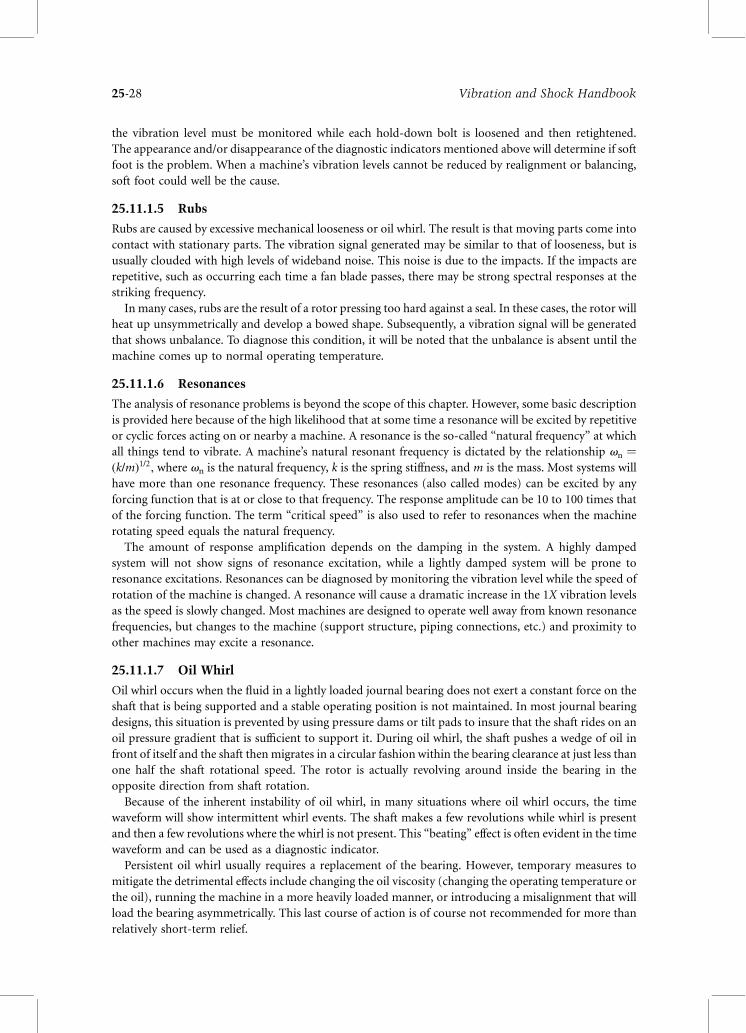
the vibration level must be monitored while each hold-down bolt is loosened and then retightened.

The appearance and/or disappearance of the diagnostic indicators mentioned above will determine if soft

foot is the problem. When a machine’s vibration levels cannot be reduced by realignment or balancing,

soft foot could well be the cause.

25.11.1.5 Rubs

Rubs are caused by excessive mechanical looseness or oil whirl. The result is that moving parts come into

contact with stationary parts. The vibration signal generated may be similar to that of looseness, but is

usually clouded with high levels of wideband noise. This noise is due to the impacts. If the impacts are

repetitive, such as occurring each time a fan blade passes, there may be strong spectral responses at the

striking frequency.

In many cases, rubs are the result of a rotor pressing too hard against a seal. In these cases, the rotor will

heat up unsymmetrically and develop a bowed shape. Subsequently, a vibration signal will be generated

that shows unbalance. To diagnose this condition, it will be noted that the unbalance is absent until the

machine comes up to normal operating temperature.

25.11.1.6 Resonances

The analysis of resonance problems is beyond the scope of this chapter. However, some basic description

is provided here because of the high likelihood that at some time a resonance will be excited by repetitive

or cyclic forces acting on or nearby a machine. A resonance is the so-called “natural frequency” at which

all things tend to vibrate. A machine’s natural resonant frequency is dictated by the relationship vn ¼ðk=mÞ1=2; where vn is the natural frequency, k is the spring stiffness, and m is the mass. Most systems will

have more than one resonance frequency. These resonances (also called modes) can be excited by any

forcing function that is at or close to that frequency. The response amplitude can be 10 to 100 times that

of the forcing function. The term “critical speed” is also used to refer to resonances when the machine

rotating speed equals the natural frequency.

The amount of response amplification depends on the damping in the system. A highly damped

system will not show signs of resonance excitation, while a lightly damped system will be prone to

resonance excitations. Resonances can be diagnosed by monitoring the vibration level while the speed of

rotation of the machine is changed. A resonance will cause a dramatic increase in the 1X vibration levels

as the speed is slowly changed. Most machines are designed to operate well away from known resonance

frequencies, but changes to the machine (support structure, piping connections, etc.) and proximity to

other machines may excite a resonance.

25.11.1.7 Oil Whirl

Oil whirl occurs when the fluid in a lightly loaded journal bearing does not exert a constant force on the

shaft that is being supported and a stable operating position is not maintained. In most journal bearing

designs, this situation is prevented by using pressure dams or tilt pads to insure that the shaft rides on an

oil pressure gradient that is sufficient to support it. During oil whirl, the shaft pushes a wedge of oil in

front of itself and the shaft then migrates in a circular fashion within the bearing clearance at just less than

one half the shaft rotational speed. The rotor is actually revolving around inside the bearing in the

opposite direction from shaft rotation.

Because of the inherent instability of oil whirl, in many situations where oil whirl occurs, the time

waveform will show intermittent whirl events. The shaft makes a few revolutions while whirl is present

and then a few revolutions where the whirl is not present. This “beating” effect is often evident in the time

waveform and can be used as a diagnostic indicator.

Persistent oil whirl usually requires a replacement of the bearing. However, temporary measures to

mitigate the detrimental effects include changing the oil viscosity (changing the operating temperature or

the oil), running the machine in a more heavily loaded manner, or introducing a misalignment that will

load the bearing asymmetrically. This last course of action is of course not recommended for more than

relatively short-term relief.


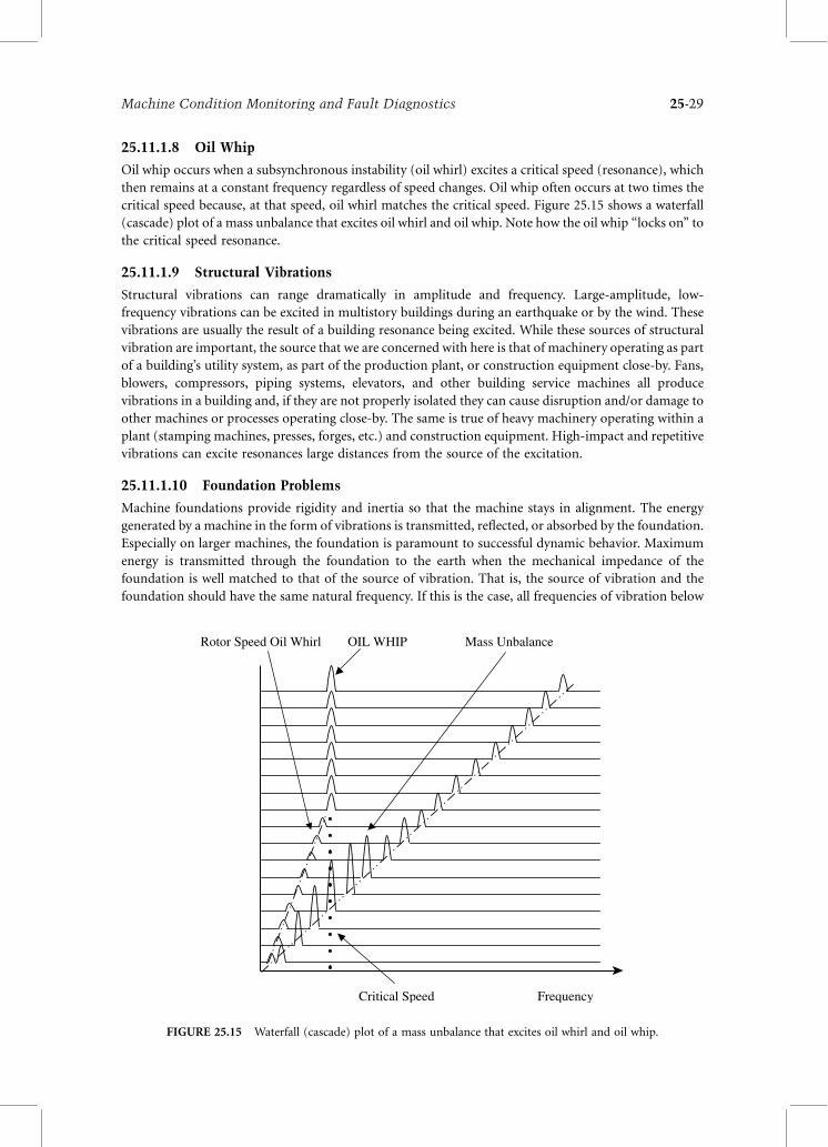
25.11.1.8 Oil Whip

Oil whip occurs when a subsynchronous instability (oil whirl) excites a critical speed (resonance), which

then remains at a constant frequency regardless of speed changes. Oil whip often occurs at two times the

critical speed because, at that speed, oil whirl matches the critical speed. Figure 25.15 shows a waterfall

(cascade) plot of a mass unbalance that excites oil whirl and oil whip. Note how the oil whip “locks on” to

the critical speed resonance.

25.11.1.9 Structural Vibrations

Structural vibrations can range dramatically in amplitude and frequency. Large-amplitude, low-

frequency vibrations can be excited in multistory buildings during an earthquake or by the wind. These

vibrations are usually the result of a building resonance being excited. While these sources of structural

vibration are important, the source that we are concerned with here is that of machinery operating as part

of a building’s utility system, as part of the production plant, or construction equipment close-by. Fans,

blowers, compressors, piping systems, elevators, and other building service machines all produce

vibrations in a building and, if they are not properly isolated they can cause disruption and/or damage to

other machines or processes operating close-by. The same is true of heavy machinery operating within a

plant (stamping machines, presses, forges, etc.) and construction equipment. High-impact and repetitive

vibrations can excite resonances large distances from the source of the excitation.

25.11.1.10 Foundation Problems

Machine foundations provide rigidity and inertia so that the machine stays in alignment. The energy

generated by a machine in the form of vibrations is transmitted, reflected, or absorbed by the foundation.

Especially on larger machines, the foundation is paramount to successful dynamic behavior. Maximum

energy is transmitted through the foundation to the earth when the mechanical impedance of the

foundation is well matched to that of the source of vibration. That is, the source of vibration and the

foundation should have the same natural frequency. If this is the case, all frequencies of vibration below

Mass UnbalanceOIL WHIPRotor Speed Oil Whirl

Critical Speed Frequency

FIGURE 25.15 Waterfall (cascade) plot of a mass unbalance that excites oil whirl and oil whip.


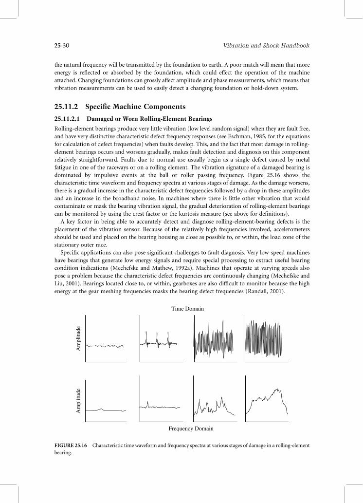
the natural frequency will be transmitted by the foundation to earth. A poor match will mean that more

energy is reflected or absorbed by the foundation, which could effect the operation of the machine

attached. Changing foundations can grossly affect amplitude and phase measurements, which means that

vibration measurements can be used to easily detect a changing foundation or hold-down system.

25.11.2 Specific Machine Components

25.11.2.1 Damaged or Worn Rolling-Element Bearings

Rolling-element bearings produce very little vibration (low level random signal) when they are fault free,

and have very distinctive characteristic defect frequency responses (see Eschman, 1985, for the equations

for calculation of defect frequencies) when faults develop. This, and the fact that most damage in rolling-

element bearings occurs and worsens gradually, makes fault detection and diagnosis on this component

relatively straightforward. Faults due to normal use usually begin as a single defect caused by metal

fatigue in one of the raceways or on a rolling element. The vibration signature of a damaged bearing is

dominated by impulsive events at the ball or roller passing frequency. Figure 25.16 shows the

characteristic time waveform and frequency spectra at various stages of damage. As the damage worsens,

there is a gradual increase in the characteristic defect frequencies followed by a drop in these amplitudes

and an increase in the broadband noise. In machines where there is little other vibration that would

contaminate or mask the bearing vibration signal, the gradual deterioration of rolling-element bearings

can be monitored by using the crest factor or the kurtosis measure (see above for definitions).

A key factor in being able to accurately detect and diagnose rolling-element-bearing defects is the

placement of the vibration sensor. Because of the relatively high frequencies involved, accelerometers

should be used and placed on the bearing housing as close as possible to, or within, the load zone of the

stationary outer race.

Specific applications can also pose significant challenges to fault diagnosis. Very low-speed machines

have bearings that generate low energy signals and require special processing to extract useful bearing

condition indications (Mechefske and Mathew, 1992a). Machines that operate at varying speeds also

pose a problem because the characteristic defect frequencies are continuously changing (Mechefske and

Liu, 2001). Bearings located close to, or within, gearboxes are also difficult to monitor because the high

energy at the gear meshing frequencies masks the bearing defect frequencies (Randall, 2001).

Time Domain

Frequency Domain

Am

plitu

deA

mpl

itude

FIGURE 25.16 Characteristic time waveform and frequency spectra at various stages of damage in a rolling-element

bearing.


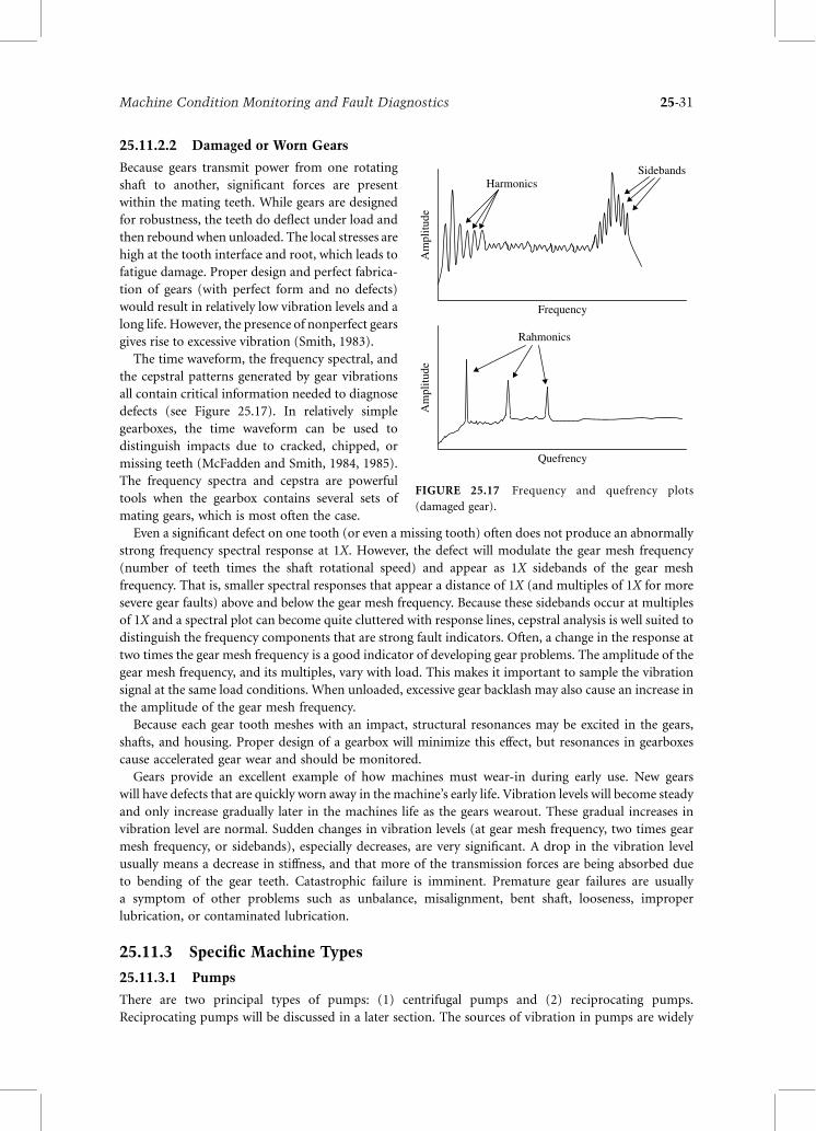
25.11.2.2 Damaged or Worn Gears

Because gears transmit power from one rotating

shaft to another, significant forces are present

within the mating teeth. While gears are designed

for robustness, the teeth do deflect under load and

then reboundwhen unloaded. The local stresses are

high at the tooth interface and root, which leads to

fatigue damage. Proper design and perfect fabrica-

tion of gears (with perfect form and no defects)

would result in relatively low vibration levels and a

long life. However, the presence of nonperfect gears

gives rise to excessive vibration (Smith, 1983).

The time waveform, the frequency spectral, and

the cepstral patterns generated by gear vibrations

all contain critical information needed to diagnose

defects (see Figure 25.17). In relatively simple

gearboxes, the time waveform can be used to

distinguish impacts due to cracked, chipped, or

missing teeth (McFadden and Smith, 1984, 1985).

The frequency spectra and cepstra are powerful

tools when the gearbox contains several sets of

mating gears, which is most often the case.

Even a significant defect on one tooth (or even a missing tooth) often does not produce an abnormally

strong frequency spectral response at 1X. However, the defect will modulate the gear mesh frequency

(number of teeth times the shaft rotational speed) and appear as 1X sidebands of the gear mesh

frequency. That is, smaller spectral responses that appear a distance of 1X (and multiples of 1X for more

severe gear faults) above and below the gear mesh frequency. Because these sidebands occur at multiples

of 1X and a spectral plot can become quite cluttered with response lines, cepstral analysis is well suited to

distinguish the frequency components that are strong fault indicators. Often, a change in the response at

two times the gear mesh frequency is a good indicator of developing gear problems. The amplitude of the

gear mesh frequency, and its multiples, vary with load. This makes it important to sample the vibration

signal at the same load conditions. When unloaded, excessive gear backlash may also cause an increase in

the amplitude of the gear mesh frequency.

Because each gear tooth meshes with an impact, structural resonances may be excited in the gears,

shafts, and housing. Proper design of a gearbox will minimize this effect, but resonances in gearboxes

cause accelerated gear wear and should be monitored.

Gears provide an excellent example of how machines must wear-in during early use. New gears

will have defects that are quickly worn away in the machine’s early life. Vibration levels will become steady

and only increase gradually later in the machines life as the gears wearout. These gradual increases in

vibration level are normal. Sudden changes in vibration levels (at gear mesh frequency, two times gear

mesh frequency, or sidebands), especially decreases, are very significant. A drop in the vibration level

usually means a decrease in stiffness, and that more of the transmission forces are being absorbed due

to bending of the gear teeth. Catastrophic failure is imminent. Premature gear failures are usually

a symptom of other problems such as unbalance, misalignment, bent shaft, looseness, improper

lubrication, or contaminated lubrication.

25.11.3 Specific Machine Types

25.11.3.1 Pumps

There are two principal types of pumps: (1) centrifugal pumps and (2) reciprocating pumps.

Reciprocating pumps will be discussed in a later section. The sources of vibration in pumps are widely

Am

plitu

de

Quefrency

Rahmonics

Am

plitu

de

Frequency

HarmonicsSidebands

FIGURE 25.17 Frequency and quefrency plots

(damaged gear).


varied. In addition to the standard mechanical problems (unbalance, misalignment, worn bearings, etc.),

problems that are particular to pumps include vane-pass frequency generating conditions (starvation,

impeller loose on the shaft, impeller hitting something) and cavitation.

Starvation occurs when not enough liquid is not present to fill each vane on the impeller every

revolution of the shaft. Pump starvation can be confused with unbalance (see Chapter 34). However, it

can be distinguished by the varying amplitude 1X vibration at constant speed and the reduced load on

the driving motor.

When the vanes on the impeller are striking something, the vane-pass frequency (the number of vanes

times the rotational speed) is excited. Because the striking causes a force on the shaft, an unbalance is also

present. The frequency spectrumwill show a response at 1X and vane-pass frequency. The time waveform

will show a high-frequency response (vane pass) riding on a frequency response at 1X. The vane-pass

frequency is in phase with the shaft speed. If the impeller is loose on the shaft, the vane-pass frequency

will be modulated by the shaft speed.

Cavitation occurs when there is sufficient negative pressure (suction) acting on the liquid in the system

that it becomes a gas (it boils). This usually takes place in localized parts of the system. Cavitation usually

occurs in a pump when the suction intake is restricted and the liquid vaporizes when coming off the

impeller. As the fluid moves past the low pressure region, the gas bubble collapses. If the collapsing

bubble is close to a solid surface, it will aggressively erode the surface. Cavitation may be caused by a local

decrease in atmospheric pressure, an increase in fluid temperature, an increase in fluid velocity, a pipe

obstruction, or abrupt change in direction. The vibration signal that results will have significant vibration

levels at 1X with harmonics and strong spectral responses at vane-pass frequency. High-frequency

broadband noise is also common. An increase in the system pressure can reduce cavitation.

Hydraulic unbalance will result if there has been poor design of suction piping (elbow close to inlet) or

poor impeller design (unsymmetrical). The vibration signal will contain high 1X axial vibration

components. Impeller unbalance is a specific form of mechanical unbalance as discussed above. High 1X

vibration levels will result. Pipe stresses result from inadequate pipe support and cause stress on the pump

casing. This may also cause misalignment. Pipe resonances can also be excited by vane-pass frequency

pressure pulsations.

Diagnosis of pump problems can be improved by installing a pressure transducer in the discharge line

of the pump. The measured pressure fluctuations can be processed in the same way as vibration signals.

The frequencies measured represent the pressure fluctuations and the amplitude is the zero-to-peak

pressure change.

25.11.3.2 Fans

Fans account for a significant number of field vibration problems due to their function and construction.

Fans move air or exhaust gases that are often laden with grease, dust, sand, ash, and other corrosive and

erosive particles (also see Chapter 34). Under these conditions, fans blades gain and lose material

resulting in the need to regularly rebalance. The level of balance must also be relatively fine because fans

often have large fan-blade diameters and operate at relatively high speeds. Fans are usually mounted on

spring/damper systems to help isolate vibrations, but they are also constructed in a relatively flexible

manner, which adds to the demands for fine balancing. Along with fine balancing requirements, typical

problems include looseness, misalignment, bent shaft, and defective bearings.

Fans also generate a strong response at blade-pass frequency (number of blades times the shaft

rotational speed). This frequency response is present during normal operation, but it can become

elevated if the blades are hitting something, the fan housing is excessively flexible, or an acoustical

resonance is present. Acoustical resonances are relatively common where large volumes of air are being

moved through large flexible ducts and/or the fan blades are of an air-foil design.

25.11.3.3 Electric Motors

Electric motors can be divided into two groups: (1) induction motors and (2) synchronous motors. A full

description will not be given here as to the differences. Like any machine, electric motors are subject to a


full range of mechanical problems, and vibrations signals can be used to detect and diagnose these

problems. Apart from the conditions described elsewhere in this section, there are some problems that

occur only in electric motors. For the sake of brevity, these problems and the vibration signals that

typically accompany them are summarized in Table 25.2.

25.11.3.4 Steam and Gas Turbines

Steam and gas turbines (and high-speed compressors) require special mention because of the high speeds

and temperatures involved. Problems on steam turbines are usually limited to looseness, unbalance,

misalignment, soft foot, resonance, and rubs. As discussed above, each of these conditions has a set of

characteristic vibration responses that allow for relatively straightforward diagnosis. However, because of

the high speeds, this type of machinery is usually designed to be lighter and less rigid than other rotating

machines. Excessive vibration can therefore lead to catastrophic failure very quickly. Because of this,

high-speed turbines and compressors are designed to closer tolerances than other types of machines, and

extra care is taken when balancing rotors. These machines also frequently operate above their first critical

speed and sometimes between their second and third critical speeds. At these speeds, the rotor becomes

quite flexible and the support bearings become very important in that they must provide the appropriate

amount of damping.

Because steam and gas turbines are supported on journal bearings, most monitoring and diagnostics

work will be based solely on proximity probe signals. While this is not a problem in and of itself,

accelerometer signals should also be taken in order to cover the higher frequencies, which are excited by

conditions such as looseness and rubs.

25.11.3.5 Compressors

Compressors act inmuch the same way as pumps, except that they are compressing some type of gas. They

come in many different sizes, but only two principal types: (1) screw-type and (2) reciprocating

compressors. Reciprocating compressorswill be discussed in a later section. Screw-type compressors have a

given number of lobes or vanes on a rotor and generate a vane-passing frequency. Screw compressors

with multiple rotors can also generate strong 1X and harmonics up to vane-pass frequency. The close

tolerances involved result in relatively highvibration levels, evenwhen themachine is in good condition. As

with pumps, signals taken from pressure transducers in the discharge line can be useful for diagnostics.

25.11.3.6 Reciprocating Machines

Reciprocating machines (gas and diesel engines, steam engines, compressors, and pumps) all have one

thing in common — a piston that moves in a reciprocating manner. These machines generally have

high overall vibration levels and particularly strong responses at 1X and harmonics, even when in

good condition. The vibrations are caused by compressed gas pressure forces and unbalance.

Vibrations at 12X may be present in four-stroke engines because the camshaft rotates at one half the

crankshaft speed.

TABLE 25.2 Mechanical Problems Particular to Electric Motors

Condition Vibration Indicator

Motor out of magnetic center High spectral response at 60 Hz

Motors with broken rotor bars High spectral response at motor running speed

and/or second harmonic

Motor with turn-to-turn shorts

in the windings

Motor runs at a slower than expected speed

(high slit frequency)

Motor out of magnetic center with

broken rotor bars or turn-to-turn

shorts in the windings

Side bands of slip frequency times the number of

poles centered around the motor running speed

and harmonics of the running speed


Many engines operate at variable speeds, which will allow the strong forcing functions to excite

resonances of the components and the mounting structure, if it is not designed in a robust manner.

Excessive vibrations in reciprocating machines usually occur due to operational problems such as

misfiring, piston slap, compression leaks, and faulty fuel injection. These problems result in elevated 12X

vibrations, if only one cylinder is affected, and a decrease in efficiency and power output. Gear and

bearing problems may also occur in reciprocating machines, but the characteristic defect frequencies for

these faults are significantly higher.

25.11.4 Advanced Fault Diagnostic Techniques

Much of the discussion in the previous sections has highlighted the fact that many machine defects

generate distinctive vibration signals. This fact has been exploited recently with the development

of a variety of different automatic fault diagnostics techniques (Mechefske and Mathew, 1992b;

Mechefske, 1995). The details of these systems will not be provided here, but the goal of automatic

diagnostics is to augment and assist, rather than replace, the vibration signal analyst. If charac-

teristic defect indicators can be detected and extracted from a vibration signal without the

intervention of a signal analyst, the analyst will have more time for other duties and will also have

access to information that may not have been uncovered through normal signal processing and

analysis.

There are, however, still many situations where machine defects do not generate distinctive vibration

signals or when the vibration signals are masked by large amounts of noise or vibrations from other

machinery. In such cases, advanced diagnostic algorithms incorporating new signal processing

techniques are currently being developed and implemented. Artificial neural networks (Timusk and

Mechefske, 2002) have been found to provide an excellent basis for detecting and diagnosing faults.

Wavelet analysis (Lin et al., 2004) and short-time Fourier transforms (STFTs) have also been shown to

effectively allow both time domain and frequency domain information to be displayed on the same plot.

This provides an opportunity to clearly see short duration transient events as well as detect faults in

machinery that is operating in nonsteady-state conditions.

References

Alfredson, R.J. 1982. A computer based system for condition monitoring, Symposium on Reliability of

Large Machines, The Institute of Engineers Australia, Sydney, pp. 39–46.

Boto, P.A., Detection of bearing damage by shock pulse measurement, Ball Bearing J., 5, 167–176, 1979.

Braun, S. 1986. Mechanical Signature Analysis: Theory and Applications, Academic Press, London.

* Analysis of the vibration signal to determine the actual type of fault present will allow for

more accurate estimation of the remaining life, the replacement parts that are needed, and

the maintenance tools, personnel, and time required to repair the machinery.* A diagnostic template can be developed for the different types of faults that are common in a

given facility or plant by listing various faults that usually develop in machinery in terms of

the forcing functions that cause them and specific machine types.* Common forcing functions include unbalance, misalignment, mechanical looseness, soft

foot, rubs, resonances, oil whirl, oil whip, structural vibrations, and foundation problems.* Specific machine components that need to be monitored include damaged or worn rolling-

element bearings and gears.* Specific machine types that can be treated as common groups include pumps, fans, electric

motors, steam and gas turbines, compressors, and reciprocating machines.


Courrech, J. 1985. New techniques for fault diagnostics in rolling element bearings, In Proceedings of the

40th Meeting of the Mechanical Failure Prevention Group, National Bureau of Standards,

Gaithersburg, MD, pp. 47–54.

Eisenmann, R.C. Sr. and Eisenmann, R.C. Jr. 1998. Machinery Malfunction: Diagnosis and Correction,

Prentice Hall, Newark.

Eschman, P. 1985. Ball and Roller Bearings, 2nd ed., Wiley, New York.

Goldman, S. 1999. Vibration Spectrum Analysis, Industrial Press, New York.

Grove, R.C. 1979. An investigation of advanced prognostic analysis techniques, Paper USARTL-TR-79-10.

Northrup Research and Technology Center, Palos Verdes, CA.

Lin, J., Zuo, M.J., and Fyfe, K.R., Mechanical fault detection based on the wavelet de-noising technique,

ASME J. Vib. Acoust., 126, 9–16, 2004.

Lyon, R.H. 1987. Machinery Noise and Diagnostics, Butterworth, Boston.

Mathew, J., Machine condition monitoring using vibration analysis, J. Aust. Acoust. Soc., 15, 7–21, 1987.

Mathew, J. and Alfredson, R.J., The condition monitoring of rolling element bearings using vibration

analysis, Trans. ASME J. Vib. Acoust. Stress Reliab. Des., 106, 447–457, 1984.

McFadden, P.D. and Smith, J.D., A model for the vibration produced by a single point defect in a rolling

element bearing, J. Sound Vib., 96, 69–77, 1984.

McFadden, P.D. and Smith, J.D., A signal processing technique for detecting local defects in a gear from

the average of the vibration, Proc. IMechE, 199, 99–112, 1985.

Mechefske, C.K., Fault detection and diagnosis in low speed rolling element bearings using inductive

inference classification, Mech. Syst. Signal Process., 9, 275–282, 1995.

Mechefske, C.K., Objective machinery fault diagnosis using fuzzy logic, Mech. Syst. Signal Process., 12,

855–864, 1998.

Mechefske, C.K. and Liu, L., Fault detection and diagnosis in variable speed machines, Int. J. Condition

Monit. Diagn. Eng. Manage., 5, 29–42, 2001.

Mechefske, C.K. and Mathew, J., Fault detection in low speed rolling element bearings, part I: the use of

parametric spectra, Mech. Syst. Signal Process., 6, 297–308, 1992a.

Mechefske, C.K. and Mathew, J., Fault detection in low speed rolling element bearings, part II: the use of

nearest neighbour classification, Mech. Syst. Signal Process., 6, 309–317, 1992b.

Mitchell, J.S. 1981. An Introduction to Machinery Analysis and Monitoring, Penwell, Los Angeles.

Mobley, R.K. 1990. An Introduction to Predictive Maintenance, Van Nostrand Reinhold, New York.

Moubray, J. 1997. Reliability Centered Maintenance, Industrial Press, New York.

Randall, R.B. 1981. A new method of modeling gear faults, ASME Annual Congress. Paper No. 81-Set-10.

Randall, R.B. 1987. Frequency Analysis, Bruel & Kjaer, Copenhagen.

Randall, R.B. 2001. Bearing diagnostics in helicopter gearboxes, Condition Monitoring and Diagnostic

Engineering Management Conference, Manchester, U.K., August 2001.

Rao, B.K.N. 1996. The Handbook of Condition Monitoring, Elsevier, Oxford.

Reeves, C.W. 1999. The Vibration Monitoring Handbook, Coxmoor, Oxford.

Smith, J.D. 1983. Gears and Their Vibrations, Marcel Dekker, New York.

Taylor, J.I. 1994. The Vibration Analysis Handbook, Vibration Consultants, Tampa.

Timusk, M. and Mechefske, C.K. 2002. Applying neural network based novelty detection to industrial

machinery, 6th International Conference on Knowledge-Based Intelligent Information Engineering

Systems, Crema, Italy, November 2002.

Wowk, V. 1991. Machinery Vibration: Measurements and Analysis, McGraw-Hill, New York.


Documents

Machine Condition Monitoring and Fault Diagnostics · Vibration Meters † Data Collectors ... diagnostics is div ided into sections that focus on different forcing functions, spec