MacAll

Lecture Notes for Macro 2 2001 (first year PhDcourse in Stockholm)

Paul Soderlind1

June 2001 (some typos corrected later)

1University of St. Gallen and CEPR. Address: s/bf-HSG, Rosenbergstrasse 52, CH-9000 St.Gallen, Switzerland. E-mail: [email protected]. Document name: MacAll.TeX.

Contents

1 Money Demand (and some Supply) 41.1 Money Supply . . . . . . . . . . . . . . . . . . . . . . . . . . . . . . 41.2 Overview of Money Demand . . . . . . . . . . . . . . . . . . . . . . 41.3 Money Demand: A General Equilibrium Model with Money in the

Utility Function . . . . . . . . . . . . . . . . . . . . . . . . . . . . . 71.4 The Mechanics of Money Supply∗ . . . . . . . . . . . . . . . . . . . 16

2 The Price of Money 242.1 UIP, Fisher Equation, and the Expectations Hypothesis of the Yield

Curve . . . . . . . . . . . . . . . . . . . . . . . . . . . . . . . . . . 242.2 The Price Level as an Asset Price: Cagan’s (1956) Model with Ratio-

nal Expectations . . . . . . . . . . . . . . . . . . . . . . . . . . . . . 252.3 A Simple Model of Exchange Rate Determination . . . . . . . . . . . 31

A Derivations of the Pricing Relations 38A.1 A Real Bond . . . . . . . . . . . . . . . . . . . . . . . . . . . . . . 40A.2 A Nominal Bond . . . . . . . . . . . . . . . . . . . . . . . . . . . . 40A.3 A Nominal Foreign Bond . . . . . . . . . . . . . . . . . . . . . . . . 41A.4 Real Effects of Money? . . . . . . . . . . . . . . . . . . . . . . . . . 41A.5 Empirical Evidence on the Pricing Relations . . . . . . . . . . . . . . 42

3 Money and Sticky Prices: A First Look 453.1 Basic Models of the Effects of Monetary Policy Surprises . . . . . . . 453.2 “Money and Wage Contracts in an Optimizing Model of the Business

Cycle,” by Benassy . . . . . . . . . . . . . . . . . . . . . . . . . . . 463.3 “Money and the Business Cycle,” by Cooley and Hansen . . . . . . . 56

1

3.4 X Sticky Wages or Sticky Prices? . . . . . . . . . . . . . . . . . . . . 61

4 Money in Models of Monopolistic Competition 634.1 Monopolistic Competition . . . . . . . . . . . . . . . . . . . . . . . 63

5 Money and Price Setting 695.1 Dynamic Models of Sticky Prices . . . . . . . . . . . . . . . . . . . 695.2 Aggregation of One-Sided Ss Rule: A Counter-Example to 1M →

1Y ∗ . . . . . . . . . . . . . . . . . . . . . . . . . . . . . . . . . . . 80

A Summary of Solution Method for Linear RE Models 81A.1 Summary . . . . . . . . . . . . . . . . . . . . . . . . . . . . . . . . 81A.2 Special Case: Scalar Second Order Equation . . . . . . . . . . . . . . 82A.3 An Alternative for the Scalar Second Order Equation: The Factoriza-

tion Method . . . . . . . . . . . . . . . . . . . . . . . . . . . . . . . 84

B Calvo’s Model: An Alternative Derivation 85

6 Monetary Policy 886.1 The IS-LM Model . . . . . . . . . . . . . . . . . . . . . . . . . . . . 886.2 The Barro-Gordon Model . . . . . . . . . . . . . . . . . . . . . . . . 916.3 Recent Models for Studying Monetary Policy . . . . . . . . . . . . . 97

A Derivations of the Aggregate Demand Equation 104

7 Empirical Measures of the Effect of Money on Output 1067.1 Some Stylized Facts about Money, Prices, and Exchange Rates . . . . 1067.2 Early Studies of the Effect of Money on Output . . . . . . . . . . . . 1077.3 Early Monetarist Studies of the Effect of Money on Output . . . . . . 1087.4 Unanticipated or Anticipated Money∗ . . . . . . . . . . . . . . . . . 1157.5 VAR Studies . . . . . . . . . . . . . . . . . . . . . . . . . . . . . . . 1167.6 Structural Models of Monetary Policy . . . . . . . . . . . . . . . . . 119

0 Reading List 1230.1 Money Supply and Demand . . . . . . . . . . . . . . . . . . . . . . 1230.2 Price Level and Nominal Assets . . . . . . . . . . . . . . . . . . . . 123

2

0.3 Money and Prices in RBC Models . . . . . . . . . . . . . . . . . . . 1240.4 Money and Monopolistic Competition . . . . . . . . . . . . . . . . . 1240.5 Sticky Prices . . . . . . . . . . . . . . . . . . . . . . . . . . . . . . 1250.6 Monetary Policy . . . . . . . . . . . . . . . . . . . . . . . . . . . . . 1250.7 Empirical Measures of the Effect of Money on Output . . . . . . . . . 1260.8 The Transmission Mechanism from Monetary Policy to Output . . . . 126

3

1 Money Demand (and some Supply)

Main references: Romer (1996) (Romer), Blanchard and Fischer (1989) (BF), Obstfeldtand Rogoff (1996) (OR), and Walsh (1998).

1.1 Money Supply

References: Burda and Wyplosz (1997) 9, OR 8.7.6 and Appendix 8B, and Mishkin(1997).

The really short version: the central bank can control either some monetary aggregateor an interest rate or the exchange rate. How they do that is typically not very importantfor most macroeconomic questions. Still, this is discussed in Section 1.4. Why they do it,that is, the monetary policy, is much more important—and something we will discuss atlength later.

1.2 Overview of Money Demand

1.2.1 Money in Macroeconomics

Roles of money: medium of exchange, unit of account, and storage of value (often domi-nated by other assets).

Money is macro model is typically identified with currency which gives no interest.The liquidity service of money ( medium of exchange) is emphasized, rather than store ofvalue or unit of account.

1.2.2 Traditional money demand equations

References: Romer 5.2, BF 4.5, OR 8.3, Burda and Wyplosz (1997) 8.The standard money demand equation

lnMt

Pt= constant + ψ ln Yt − ωit (1.1)

4

are used in many different models, for instance as the LM curve is IS-LM models. Mt in(1.1) is often a money aggregate like M1 or M3. In most of the models on this course, wewill assume that the central bank have control over this aggregate.

1.2.3 Money Demand and Monetary Policy

There are many different models for why money is used. The common feature of thesemodels is that they all generate something pretty close to (1.1). But why is this broadermoney aggregate related to the monetary base, which the central bank may control? Shortanswer: the central bank creates a demand for narrow money by forcing banks to hold it(reserve requirements) and by prohibiting private substitutes to narrow money (banks arenot allowed to print bills).

The idea behind central bank interventions is to affect the money supply. However,most central banks use short interest rates as their operating target. In effect, the centralbank has monopoly over supply over narrow money which allows it to set the short interestrate, since short debt is a very close substitute to cash. In terms of (1.1), the central bankmay set it , which for a given output and price level determines the money supply as aresidual.

1.2.4 Applied money demand equations

Reference: Goldfeld and Sichel (1990).Applied money demand equations often take the form

lnMt

Pt= b0 + b1 ln Yt + b2it + b3 ln

Mt−1

Pt−1+ b4 ln

Pt

Pt−1+ ut . (1.2)

where Mt is nominal money holdings, Pt the price level, Yt some measure of economicactivity, and it the net nominal interest rate (like 0.07). The inclusion of Mt−1/Pt−1 andPt/Pt−1 is thought to capture partial adjustment effects due to adjustment costs of eithernominal (b4 6= 0) or real money balances (b4 = 0).

For instance, the estimate for Germany (69:1-85:4) reported by Goldfeld and Sichel(1990) is {b1, b2, b3, b4} = {0.3,−0.5, 0.7,−0.7}. (They interest rate used in their esti-mation is in percentages, that is, like 7 instead of the 0.07 used here, so I have scaled theirb2 = −0.005 by 100.)

5

In general, this type of equation worked fine until 1975, overpredicted money demandduring the late 1970s, and underpredicted money demand in the early 1980s. Financialinnovations? (1.2) has been refined in various ways. Various disaggregated money mea-sures have been tried, a wealth of different interest rates and alternative costs have beenused, the income variable has been disaggregated, and fairly free adjustment models havebeen tried (error correction models). Single equation estimation of (1.2) presumes thatthis is a true demand function, with monetary authorities setting the interest rate, and withthe other right hand side variables being predetermined.

1.2.5 Different Ways to Introduce Money in Macro Models

Reference: OR 8.3 and Walsh (1998) 2.3 and 3.3.The money in the utility function (MIU) model just postulates that real money balances

enter the utility function, so the consumer’s optimization problem is

max{Ct ,Mt }

∞

t=0

∞∑t=0

β tu(

Ct ,Mt

Pt

). (1.3)

One motivation for having the real balances in the utility function is that having cash maysave time in transactions. The correct utility function would then be u

(Ct , L − Lshopping

t

),

where Lshoppingt is a decreasing function of Mt/Pt .

Cash-in-advance constraint (CIA) means that cash is needed to buy (some) goods, forinstance, consumption goods

PtCt ≤ Mt−1, (1.4)

where Mt−1 was brought over from the end of period t − 1. Without uncertainty, thisrestriction must hold with equality since cash pays no interest: no one would accumulatemore cash than strictly needed for consumption purposes since there are better investmentopportunities. In stochastic economies, this may no longer be true.

The simple CIA constraint implies that “money demand equation” does not includethe nominal interest rate. If the utility function depends on consumption only, then allrates of inflation gives the same steady state utility. This stands in sharp contrast to theMIU model, where the optimal rate of inflation is minus one times the real interest rate(to get zero nominal interest rate). However, this is not longer true if the cash-in-advanceconstraint applies only to a subset of the arguments in the utility function. For instance, if

6

we introduce leisure or credit goods.Shopping-time models typically have a utility function is terms of consumption and

leisure∞∑

s=0

βsU (Ct , 1 − lt − nt) , (1.5)

where lt is hours worked, and nt hours spent on shopping (supposed to give disutility).The latter is typically modelled as some function which is increasing in consumption anddecreasing in cash holdings

1.3 Money Demand: A General Equilibrium Model with Money inthe Utility Function

Reference: BF 4.5; OR 8.3; Walsh (1998) 2.3; and Lucas (2000)

1.3.1 Model Setup

The consumer’s optimization problem is

max{Ct ,Mt }

∞

t=0

∞∑t=0

β tu(

Ct ,Mt

Pt

)(1.6)

subject to the real budget constraint

Kt+1 +Mt

Pt= (1 + rt) Kt +

Mt−1

Pt+ wt − Ct − Tt , (1.7)

where rt is the (net) real interest rate (from investing in t − 1 and receiving the return int), and wt the real wage rate. Labor supply is normalized to one. The consumer rents hiscapital stock to competitive firms in each period. Tt denotes lump sum taxes.

Production is given by a production function with constant returns to scale

Yt = F (Kt , L t) , (1.8)

and there is perfect competition in the product and factor markets. The firms rent capitaland labor from the households and make zero profits.

I assume perfect foresight in order to simply the algebra somewhat. It is straightfor-ward to derive the same results in a stochastic setting, at least if we assume that variances

7

and covariances do not depend on the level of the other variables.

1.3.2 Optimal Consumption and Money Holdings

Use (1.7) in (1.6) to get the unconstrained problem for the consumer

max{Kt+1,Mt}

∞

t=0

∞∑t=0

β tu[(1 + rt) Kt +

Mt−1

Pt+ wt − Tt − Kt+1 −

Mt

Pt,

Mt

Pt

]. (1.9)

The first order condition for Kt+1 is

uC

(Ct ,

Mt

Pt

)= (1 + rt+1) βuC

(Ct+1,

Mt+1

Pt+1

), (1.10)

which is the traditional Euler equation for real bonds (with uncertainty we need to takethe expected value of the right hand side, conditional on the information in t). It wouldalso hold for any other financial asset.

The first order condition for Mt is

uC

(Ct ,

Mt

Pt

)= uM/P

(Ct ,

Mt

Pt

)+ βuC

(Ct+1,

Mt+1

Pt+1

)Pt

Pt+1. (1.11)

If money would not enter the utility function, then this is a special case of (1.10) since thereal gross return on money is Pt/Pt+1. It is not obvious, however, that we get an interiorsolution to money holdings unless money gives direct utility.

The left hand side of (1.11) is the marginal utility lost because some resources aretaken from time t consumption, and the right hand side is the marginal utility gained byhaving more cash today and the extra consumption this allows tomorrow (cash providesutility and is also a form of saving, whose purchasing power depends on the inflation).

Substitute for βuC (Ct+1,Mt+1/Pt+1) from (1.10) in (1.11) and rearrange to get

uC

(Ct ,

Mt

Pt

)(1 −

11 + rt+1

Pt

Pt+1

)= uM/P

(Ct ,

Mt

Pt

). (1.12)

The Fisher equation is

1 + it = Et (1 + rt+1)Pt+1

Pt, (1.13)

where the convention is that the nominal interest rate is dated t since it is known as of t .

8

Under perfect foresight, (1.12) can then be written

it

1 + it= uM/P

(Ct ,

Mt

Pt

)/uC

(Ct ,

Mt

Pt

), (1.14)

which highlights that the nominal interest rate is the relative price of the “money services”we get by holding money one period instead of consuming it. Note that (1.14) is a rela-tion between real money balances, the nominal interest rate, and an activity level (hereconsumption), which is very similar to the LM equation.

Example 1 (Explicit money demand equation from Cobb-Douglas/CRRA.) Let the utility

function be

u(

Ct ,Mt

Pt

)=

11 − γ

[Cα

t

(Mt

Pt

)1−α]1−γ

,

in which case (1.14) can be written

Mt

Pt= Ct

1 − α

α

1 + it

it,

which is decreasing in it and increasing in Ct . This is quite similar to the standard

money demand equation (1.1). Take logs and make a first-order Taylor expansion of

ln [(1 + it) / it ] around iss

lnMt

Pt= constant + ln Ct −

1iss (1 + iss)

it .

Compared with the money demand equation (1.1), ψ ln Yt is replaced by ln Ct and ω =

1/ [iss (1 + iss)]. If iss = 5%, then ω ≈ 20, which appears to be very high compared to

empirical estimates.

Example 2 (Explicit money demand equation from Lucas (2000). Let the utility function

be

u(

Ct ,Mt

Pt

)=

11 − γ

[Ct

(1 + B

Ct

Mt/Pt

)−1]1−γ

,

9

in which case (1.14) can be written

it

1 + it=

(Ct

Mt/Pt

)2

B, or

Mt

Pt= Ct B1/2

(it

1 + it

)−1/2

,

which can be written (approximately) on the same form as (1.1)

lnMt

Pt≈ constant + ln Ct −

12

it

iss (1 + iss).

This gives a value of the ω in the money demand equation (1.1) which is only half of that

in Example 1.

1.3.3 General Equilibrium with MIU

We now add a few equations to close the MIU model in a closed economy. The govern-ment budget is assumed to be in balance in every period (not restrictive since Ricardianequivalence holds in this model)

−Ts =Ms − Ms−1

Ps, (1.15)

so the seigniorage (right hand side) is distributed as lump sum transfers (negative taxes).Note that this is taken as given by each individual agent.

Competitive factor markets, constant returns to scale, and a fixed labor equal to one(recall that is was not part of the utility function) give

rt =∂F (Kt , 1)

∂K, and (1.16)

wt = F (Kt , 1)− Kt∂F (Kt , 1)

∂K.

(This follows from that w = ∂F/∂L and r = ∂F/∂K and that constant returns to scaleimplies F = L∂F/∂L + K∂F/∂K .)

In general, the price level is determined jointly with the rest of the dynamic equilib-rium. In special cases, as with log utility and complete depreciation of capital (as in themodel of Benassy (1995)) there is a closed form solution. However, in most cases, theequilibrium must be computed with numerical methods.

10

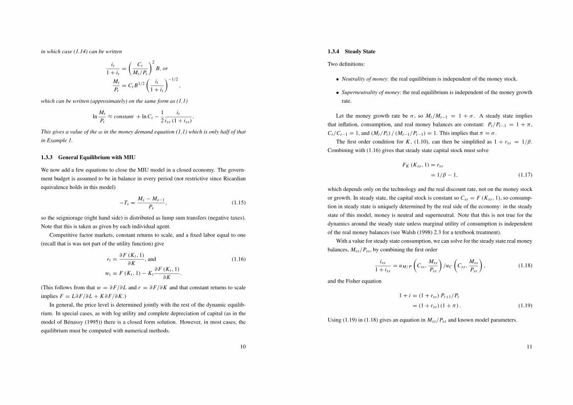
1.3.4 Steady State

Two definitions:

• Neutrality of money: the real equilibrium is independent of the money stock.

• Superneutrality of money: the real equilibrium is independent of the money growthrate.

Let the money growth rate be σ , so Mt/Mt−1 = 1 + σ . A steady state impliesthat inflation, consumption, and real money balances are constant: Pt/Pt−1 = 1 + π ,Ct/Ct−1 = 1, and (Mt/Pt) / (Mt−1/Pt−1) = 1. This implies that π = σ .

The first order condition for K , (1.10), can then be simplified as 1 + rss = 1/β.Combining with (1.16) gives that steady state capital stock must solve

FK (Kss, 1) = rss

= 1/β − 1, (1.17)

which depends only on the technology and the real discount rate, not on the money stockor growth. In steady state, the capital stock is constant so Css = F (Kss, 1), so consump-tion in steady state is uniquely determined by the real side of the economy: in the steadystate of this model, money is neutral and superneutral. Note that this is not true for thedynamics around the steady state unless marginal utility of consumption is independentof the real money balances (see Walsh (1998) 2.3 for a textbook treatment).

With a value for steady state consumption, we can solve for the steady state real moneybalances, Mss/Pss , by combining the first order

iss

1 + iss= uM/P

(Css,

Mss

Pss

)/uC

(Css,

Mss

Pss

), (1.18)

and the Fisher equation

1 + i = (1 + rss) Pt+1/Pt

= (1 + rss) (1 + π) . (1.19)

Using (1.19) in (1.18) gives an equation in Mss/Pss and known model parameters.

11

1.3.5 The Welfare Cost of Inflation

The welfare cost of inflation is typically analyzed for the steady state, since we can thenmake use of the superneutrality of money. The growth rate of money, and therefore theinflation rate and nominal interest rate, can then be changed without affecting the realequilibrium.

The welfare loss from a higher nominal interest rate is often measured as the extraconsumption needed in order to achieve the same utility as in the case with lower interestrate. The approach is typically to find the money demand function which expresses realmoney balances as a function of the consumption level and the nominal interest rate M

P =

f (i,C), and calculate utility as the value of the period utility function u [C, f (i,C)].If C = 1 in steady state, a certain interest rate i0 gives the utility u

[1, f

(i0, 1

)]. The

welfare loss from another nominal interest rate, i1, is the value of C which solves

u[1, f

(i0, 1

)]= u

[C, f

(i1,C

)]. (1.20)

This value of C is the compensation that the consumers need to be as well off with theinterest rate i1 as with i0. Note that C − 1 can be interpreted as the percentage change inconsumption needed to compensate for the higher nominal interest rate.

Example 3 (Welfare loss with Cobb-Douglas/CRRA.) From Example 1, the utility at the

nominal interest rate i is

u [C, f (i,C)] =1

1 − γ

[Cα

(C

1 − α

α

1 + ii

)1−α]1−γ

.

Consider a steady state where C = 1 and suppose that inflation is zero, so i = r . For

instance, to get the same utility as at C = 1 and i = 3%, u [1, f (0.03, 1)], then con-

sumption must be (1.03/ (1 + i)

0.03/ i

)1−α

= C.

Figure 1.1 illustrates the result for α = 0.99.

Example 4 (Welfare loss from Lucas (1994).) From Example 2 we get

u [C, f (i,C)] =1

1 − γ

C

(1 + B1/2

(it

1 + it

)1/2)−1

1−γ

.

12

3 4 5 6 7 8 9 100

0.5

1

1.5

Money in utility function: cost of i>3%

Nominal interest rate, %

Fra

ctio

n o

f co

nsu

mp

tion

, %

Cobb−Douglas, α=0.99

Lucas, B=0.0018

Figure 1.1: Utility loss, in terms of consumption, of inflation in two MIU models.

To get the same utility as with C = 1 and i = 3% consumption must be

1 + B1/2(

i1+i

)1/2

1 + B1/2(0.03

1.03

)1/2 = C.

Figure 1.1 illustrates the result for B = 0.0018 (Lucas’ point estimate).

Also a cash-in-advance model (see, for instance, Cooley and Hansen (1989)) can gen-erate welfare costs of inflation (more precise: of a non-zero nominal interest rate) if thecash-in-advance restriction applies only to a subset of the arguments in the utility func-tion. A positive inflation acts like a tax on those goods that must be paid in cash, andthereby creates a distortion.

Friedman’s Rule for Optimal Money Supply

Reference: Romer 9.8, BF 4.5.Friedman suggested a money rate growth which would set the nominal interest rate to

zero and thereby saturate money demand. The idea is that bills are (virtually) costless toprint and it has a (utility) value for agents, so why not give them as much as they wouldpossibly would like to have?

13

We know that the steady states of the real variables is unaffected by the inflation rate(see above), so if we concentrate attention to the steady state, then (1.14) tells us thatconsumers are satiated with real money balances if uM/P = 0, that is, if i = 0.

By the Fisher equation (1.13) this means that the monetary policy should set (1 + rt) Pt+1/Pt =

1, so the rate of deflation should equal the real interest rate. In this way, holding cash givesthe same return as a real bond, so savers will be happy to keep large real money balancesand to get the utility out of it.

In steady state, inflation equals the money growth rate, so a deflation requires a shrink-ing money supply, which means that seigniorage is negative—see (1.15). In this setting,this is compensated by lump-sum taxes, which highlights the assumption that the gov-ernment revenues from the inflation tax is either wasted or can be raised in other, non-distortive, ways. If, instead, a certain revenue must be raised and the alternative taxes aredistortive, then it may no longer be optimal with a zero inflation rate. See Walsh (1998).

If the utility function is separable in consumption and real money balances, then thisresult hold in general, not just in steady state.

The Welfare Cost of Inflation - Other Arguments

Reference: Fischer (1996), Romer 9.8, Driffil, Mizon, and Ulph (1990), and Walsh (1998)4.5-4.6.

1. Inflation raises the effective capital income tax (subsidy), since the nominal return(loss) is taxed (part of which is just compensation for inflation). The real net of taxreturn is

rnet= (1 − τ) i − π

= (1 − τ) r − τπ, (1.21)

where the Fisher relation gives i = r + Eπ and we assume that π = Eπ . Thisdistorts the savings decision. Some calculation for the US (Feldstein, NBER, 1996)suggest that this effect is large (twice as large as the effect on government revenues).Counter-argument: a lower inflation and therefore lower government revenues fromcapital income taxation is likely to bring higher tax rates.

2. Costs of price adjustments and indexation.

14

3. Some empirical evidence that really high inflation is bad for growth. It is (boththeoretically and empirically) unclear if zero inflation is better for growth than 5%inflation.

4. Seigniorage is low for most OECD countries (less than one percent of GDP, see OR8.2).

5. Low inflation means that it will be hard to drive down the real interest really low tostimulate output. (The nominal interest rates cannot be negative since the nominalreturn on cash is zero.).

6. Variable inflation may lead to large inflation surprises which redistribute wealth,increases uncertainty (affects savings in which way?), and increases the informationcosts.

1.3.6 The Relation to Traditional Macro Models

Equation (1.14) is a money demand equation, which in many cases can be approximatedby

ln Mt − ln Pt = γ1 ln Ct − γ2it , (1.22)

which is a traditional LM equation.When the utility function is separable in consumption and real money balances, then

the optimality condition for consumption (1.10) can often be approximated by

−γ ln Ct = ln (1 + rt+1)+ γ ln Ct+1, (1.23)

where consumption growth is related to the real interest rate. From the Fisher equation,we can replace ln (1 + rt+1) by it−Et (ln Pt+1 − ln Pt). This is clearly reminiscent of anIS equation.

1.3.7 The Price Level

The price level is determined simultaneously with all other variables, and there is typicallyno closed form solution.

In the special case where the utility function in (1.6) is separable, so the Euler equationfor consumption (1.10) is unaffected by real money balances, and where money supply

15

is exogenous is might be possible to arrive at an analytical expression for the price level.In this case, we can solve for the real equilibrium (consumption, real interest rates, etc)without any reference to money supply. The price level can then be found by solving(1.11) and information about money supply. This is an example of a classical dichotomy.

Example 5 (Solving for the price level.) Use the approximate Fisher equation, it =Et ln Pt+1−

ln Pt + rt+1, in the approximate money demand equation in Example 1

ln Mt − ln Pt = a + ln Ct −1

iss (1 + iss)(Et ln Pt+1 − ln Pt + rt+1) ,

and rewrite as

ln Ptiss (1 + iss)+ 1

iss (1 + iss)= −a − ln Ct + ln Mt +

1iss (1 + iss)

rt+1 +1

iss (1 + iss)Et ln Pt+1,

which is a forward looking difference equations for ln Pt in terms of the “exogenous”

variables ln Ct , ln Mt , and rt+1.

1.4 The Mechanics of Money Supply∗

References: Burda and Wyplosz (1997) 9, OR 8.7.6 and Appendix 8B, and Mishkin(1997).

The short version: the central bank can control either some monetary aggregate or aninterest rate or the exchange rate. This section is about how they do that, even if this isnot particularly important for most macroeconomic issues. Why they do it, that is, themonetary policy, is much more important—and something we will return to later.

1.4.1 Operating Procedures of the Central Bank

Suppose demand for the monetary base is decreasing in the nominal interest rate. Supposethe central bank does no interventions at all. Shifts in the demand curve for money willthen lead to movements in the nominal interest rate. Alternatively, suppose the centralbank announces a discount rate where any bank can lend/borrow unlimited amounts. Thiswill fix the interest rate and any shifts in the demand curve leads to movements in themonetary base (as the banks are free to borrow reserves and currency at the fixed rate).Finally, it is possible to strike a compromise between these two extremes letting banks

16

M

i

M

i

M

i

supply

supply

supply

a. Interest rule

b. Money rule

c. Mixture

Figure 1.2: Partial equilibrium on money market

lend at increasing interest rates. This effectively creates an upward sloping supply curvefor the monetary base. This is illustrated in Figure 1.2.

1.4.2 Money Supply and Budget Accounting

Money supply has a direct effect on government finances. Consider the consolidated gov-ernment sector (here interpreted as treasury plus central bank). The real budget identityis

G t +Bt−1

Pt(1 + it−1)+

Mt−1

Pt= Tt +

Bt

Pt+

Mt

Pt, (1.24)

where G t and Tt are real government expenditures revenues, respectively, Bt is nominaldebt, it the nominal interest rate, Mt is the monetary base (the central bank liabilities),and Pt the price level.

17

Assume the Fisher equation holds, so the nominal interest rate is

1 + it−1 = Et−1 (1 + rt)Pt

Pt−1, (1.25)

where rt is the real interest rate. The convention is that the nominal interest rate is datedt − 1 since it is known as of t − 1. To simplify, assume rt is known in t − 1. We then getfrom (1.25) that the real debt in t is

Bt

Pt= G t − Tt + (1 + rt)

Bt−1

Pt−1

Pt−1

PtEt−1

Pt

Pt−1−

Mt − Mt−1

Pt. (1.26)

Consider the case where real government expenditures and tax revenues are unaffectedby monetary policy (money is neutral), and where the central bank increases money sup-ply, Mt > Mt−1. This drives down the real value of government debt, Bt/Pt in twoways. First, the real revenues from money creation (printing), called seigniorage, is(Mt − Mt−1)/Pt . Second, the money supply increase will probably increase the pricelevel. If this increase is unanticipated, then actual inflation exceeds expected inflation,Pt−1/PtEt−1(Pt/Pt−1) < 1, so the real value of government debt brought over from t −1decreases.

1.4.3 Money Aggregates and the Balance Sheet of the Central Bank

The liabilities of the central bank are currency (Cu) plus banks reserves (Re) depositedin the central bank, the assets are the foreign exchange reserve, the holding of domesticbonds, and perhaps gold

Balance Sheet of Central BankAssets LiabilitiesDomestic bonds Currency (Cu)Foreign currency Reserve deposits (Re)Foreign bonds Net worthGold

18

1.4.4 Reserve Requirements and Deposits

Money stock, M , is currency, Cu, plus deposits, D, (also called “inside money” since it isgenerated inside the private banking system)

M = Cu + D. (1.27)

Suppose that private banks (because of reserve requirements or prudence) hold thefraction r of deposits, D, in reserves, Re. This means that an increase in reserves, 1Re,allows the bank to increase deposits with the reserve multiplier, 1/r ,

1D =1Re

r. (1.28)

These new deposits may be lent to someone (an thereby bring in profits to the bank,assuming the lending rate is above the deposit rate). Note that if r goes to zero, then thecentral bank cannot control the creation of new deposits by affecting the availability ofreserves.

Reserve requirements mean that a private bank must hold a fraction (usually a fewpercentage) of the (checkable) deposits in either cash (in the vault) or as reserves withthe central bank. This fraction is often specified as an average over some period (twoweeks in the US). Suppose a bank needs to get more reserves (maybe depositors withdrewmoney during the preceding week). It can then either sell some assets, borrow from otherbanks (“federal funds” market in the US), or borrow from the central bank (at the Fed’s“discount window” in the US). Note that borrowing from the central bank is effectivelya decrease (as long as the loan lasts) in the reserve requirement. Therefore somethinghas to be done to make the reserve requirements bite in spite of the possibility to borrowfrom the central bank. This is typically a penalty rate for these loans, or some kind ofadministrative rationing of loans.

It is the fact that r < 1 that makes banks different from other financial institutions.To see why, suppose r = 1. Then all deposits would have to be kept as reserves andcouldn’t be used for lending. Consequently, any lending has to be done from the banksown capital. In this sense, the bank is not an intermediary any more and cannot “createmoney.”

The money stock deposits discussed above can be interpreted/measured in differentways. The most common monetary aggregates are: M1 (currency, travellers’ checks,

19

checkable deposits); M2 (M1 plus small denomination time deposits, savings deposits,money market funds, repos, Eurodollars); M3 (M2 plus large denomination time deposits,and money market funds held by institutions)

1.4.5 Interventions and the Money Multiplier

The central bank can typically not control the reserves directly, only the sum of reservesand currency (the private sector can always convert the currency into reserves and viceversa). This sum is called the monetary base (B) (also called high-powered money, M0,central bank money, or outside money since it is generated outside the private bankingsystem), is

B = Cu + Re. (1.29)

The monetary base can be increased by, for instance, an open market operation wherethe central bank buys government bonds and pays by either cash (increases Cu) or cheque(increases Re). The same effect is achieved by a foreign exchange intervention; the centralbank buys a foreign asset and pays by either cash or cheque denominated in the domesticcurrency.

Suppose private agents wants to hold the fraction c of the money stock in currency.We can then write (1.29) and (1.27) as

B = cM + r D (1.30)

M = cM + D.

The money multiplier, M divided by B, can then be written

MB

=M

Cu + Re

=D/ (1 − c)

Dc/ (1 − c)+ r D

=1

c + r (1 − c). (1.31)

The relation between money stock and monetary base is therefore

M =1

c + r (1 − c)B. (1.32)

20

c is often thought of as being determined by bank/households, so the central bank canaffect money supply by either influencing r (reserve requirements) or by changing themonetary base (interventions). The money multiplier is decreasing in fraction of currency,c, since it acts like a “leakage” from the private banking system. At c = 0, that is, whenthere is no currency, then the money multiplier is at a maximum and coincides with thereserve multiplier.

Example 6 (US data 1994, Burda and Wyplosz (1997) 9) For the US 1994 c = 0.29,

M1/M0 = 2.83, which by (1.32) should imply that r = 0.089. The reserve requirements

on demand deposits was (at least in 1995) virtually zero for small demand deposits..

Explanations: voluntary reserves (prudence or transaction purposes) and “leakages”

(deposits in nonbank financial institutions).

Example 7 (The Great Depression.) Private sector decisions can lead to important

changes in both c and r. During the Great Depression, B was not changed much (counter

to the conventional wisdom about a contractionary monetary policy), while savers with-

drew deposits from the banks and the banks increased the voluntary reserves (both c and

r increased substantially), with the result that M decreased some 30%. Fear of banks

going bust?

Example 8 (Money creation.) The central bank makes an open market purchase of

bonds. This increases the monetary base by 1B. Recall Re = r D and Cu = cM,

so according to (1.30)

B =

(c

1 − c+ r

)D.

The increase in the monetary base will therefore be split into increases in reserves and

currency according to

1Re = φ1B where φ =r (1 − c)

c + r (1 − c)

1Cu = δ1B where δ =c

c + r (1 − c).

For concreteness, assume this could happen if the central bank buys the bonds from the

(consolidated) private bank, which in turn buys some of them from savers. The extra

reserves allow the (consolidated) private bank to take extra deposits. This can be done by

21

lending money to a customer by crediting his deposit account. This extra deposit is

1D =φ

r1B

=1 − c

c + r (1 − c)1B.

Clearly,

1M = 1D +1Cu

=1

c + r (1 − c)1B,

as expected and all desired ratios are fulfilled (check this).

1.4.6 More on Interventions

Reference: ORA sterilized foreign exchange intervention is when the effects on the money supply of

a foreign exchange intervention is nullified by an open market operation; the central bankbuys foreign assets, pays with cash, but sell domestic assets (government bonds) to getthe cash back.

An intervention on the forward market is very similar to a sterilized intervention.Suppose the bank enters a forward contract to buy domestic currency tomorrow and tosell foreign currency at the same time. This decreases the supply of “domestic currencytomorrow,” that is, of domestic bonds, while increasing the supply of foreign bonds - justlike in a sterilized intervention.

It seems as if sterilized interventions can have effects on exchange rates and interestrates, but we are not sure why. Portfolio-balance effect (changing supply changes the riskpremium, but what about Ricardian equivalence?) or signalling?

Bibliography

Benassy, J.-P., 1995, “Money and Wage Contracts in an Optimizing Model of the BusinessCycle,” Journal of Monetary Economics, 35, 303–315.

Blanchard, O. J., and S. Fischer, 1989, Lectures on Macroeconomics, MIT Press.

22

Burda, M., and C. Wyplosz, 1997, Macroeconomics - A European Text, Oxford UniversityPress, 2nd edn.

Cooley, T. F., and G. D. Hansen, 1989, “The Inflation Tax in a Real Business CycleModel,” The American Economic Review, 79, 733–748.

Driffil, J., G. E. Mizon, and A. Ulph, 1990, “Costs of Inflation,” in Benjamin M. Friedman,and Frank H. Hahn (ed.), Handbook of Monetary Economics . , vol. 2, North-Holland.

Fischer, S., 1996, “Why Are Central Banks Pursuing Long-Run Price Stability,” inAchieving Price Stability, pp. 7–34. Federal Reserve Bank of Kansas City.

Goldfeld, S. M., and D. E. Sichel, 1990, “The Demand for Money,” in Benjamin M. Fried-mand, and Frank H. Hahn (ed.), Handbook of Monetary Economics, vol. 1, . chap. 8,North-Holland.

Lucas, R. E., 2000, “Inflation and Welfare,” Econometrica, 68, 247–274.

Mishkin, F. S., 1997, The Economics of Money, Banking, and Financial Markets,Addison-Wesley, Reading, Massachusetts, 5th edn.

Obstfeldt, M., and K. Rogoff, 1996, Foundations of International Macroeconomics, MITPress.

Romer, D., 1996, Advanced Macroeconomics, McGraw-Hill.

Walsh, C. E., 1998, Monetary Theory and Policy, MIT Press, Cambridge, Massachusetts.

23

2 The Price of Money


2.1 UIP, Fisher Equation, and the Expectations Hypothesis of theYield Curve

Reference: OR 8.7.1-8.7.3

2.1.1 Pricing Relations for Nominal Returns

This section gives three very important relations, which we will use in the subsequentanalysis. These relations can be stated in several different forms, but here we use thelog-linear form which fits nicely into the linear models used in most of this class.

Let it be a continuously compounded (per period) nominal interest rate on a discountbond (no coupons) traded at t and maturing at t + 1, and let πt+1 = ln(Pt+1/Pt) bethe corresponding inflation rate. The relation between nominal interest rates, real interestrates and expected inflation is

it = Etπt+1 + rrt + ϕπt , (2.1)

where rrt is a real interest rate and ϕπt a risk premium (inflation risk premium). The Fisher

equation assumes that the risk premium is zero or constant, and sometimes also that thereal interest rate is constant.

The relation between domestic interest rates, foreign interest rates (indicated by astar∗), and expected exchange rate depreciation is

it − i∗

t = Et ln (St+1/St)− ϕst , (2.2)

where St is the exchange rate (units of domestic currency per unit of foreign currency,for instance, 8 SEK per USD), and ϕs

t is a risk premium (exchange rate risk premium).

24

(The sign of the risk premium is just a matter of definition. Here ϕst > 0 means that

an investment in foreign bonds require a positive risk premium.) Uncovered interest rateparity, UIP, assumes that the risk premium is zero or constant. Both (2.1) and (2.2) havesimilar forms for multi-period investments.

Finally, let it,t+s be the continuously compounded per period nominal interest rate ona discount bond traded at t and maturing at t + s. The relation between long interest ratesand expected future short interest rates is

it,t+s =1s(Et it + Et it+1 + · · · + Et it+s−1)+ ϕi

t , (2.3)

where ϕit is a risk premium (term premium). The expectations hypothesis of interest rates

(yield curve) assumes that the risk premium is zero or constant.Derivations are given in the Appendix.

2.2 The Price Level as an Asset Price: Cagan’s (1956) Model withRational Expectations

Reference: BF 4.7 and 5.1, Romer 9.7, OR 8.2, Walsh (1998) 4.3.This classic model was first used to discuss hyperinflation. In this case prices are

driven almost entirely by the dynamics of money supply (Phillips effects and other influ-ences of real variables are of minor importance). Many hyperinflation episodes originatein the need to generate government revenues, why we will take a look at seigniorage. Thismodel also allows us to discuss the “asset pricing” aspect of the price level, and how tosolve such models.

The model is an approximation to the general equilibrium model with money in theutility function, where the real side of the economy (output, consumption, real interestrate) is kept constant.

2.2.1 Determination of the Price Level under Rational Expectations

Suppose the money demand function (LM curve) is

ln Mt − ln Pt = ψ ln Yt − ωit , with ω > 0. (2.4)

25

Prices are assumed to be completely flexible. Assume that income and the real interestrate are constant, so by the Fisher equation

it = Et(ln Pt+1 − ln Pt) + constant, (2.5)

and the money demand equation can be normalized as

ln Mt − ln Pt = −ω (Et ln Pt+1 − ln Pt) . (2.6)

These assumptions could either be motivated by that this is a steady state situation (generalequilibrium with MIU) or that we want to look at hyperinflation, where movements in thereal interest rate and output are of trivial importance compared with the movements in themoney stock.

Remark 9 (The price of money) Note that if one unit of the good costs Pt units of money,

then one unit of money costs Ft = 1/Pt units of goods. We can then rewrite (2.6) as

ln Ft = − ln Mt + ω (Et ln Ft+1 − ln Ft) .

This says that the price of money equals a dividend, − ln Mt , and a discounted capital

gain. To see that − ln Mt is like a dividend, suppose utility is U (C,M/P) = u1(C) +

ln M/P, then UM = 1/M. We could therefore think of − ln Mt as an approximation of

the marginal utility of money.

Rewrite (2.6) as

ln Pt = (1 − η) ln Mt + ηEt ln Pt+1, with η = ω/ (1 + ω) < 1. (2.7)

The price level today depend on the money supply, but also on the expected price leveltomorrow. If the price level tomorrow is expected to be very high, then currency willbe worth little tomorrow (the value of money in terms of goods is 1/Pt ). Like any otherasset, the value of money will then decrease already today, which means that Pt increases.

Remark 10 (Law of iterated expectations.) We must have

EtEt+1 ln Pt+2 = Et ln Pt+2,

since the information set in t is a subset of the information set in t + 1. (Senility is not

allowed.)

26

Substituting for Et ln Pt+1 in (2.7) gives

ln Pt = (1 − η) ln Mt + ηEt[(1 − η) ln Mt+1 + ηEt+1 ln Pt+2

]︸︷︷︸ln Pt+1

, (2.8)

= (1 − η) ln Mt + η (1 − η)Et ln Mt+1 + η2Et ln Pt+2, (2.9)

where we use the law of iterated expectations. By continuing the substitution we end upwith

ln Pt = (1 − η)

K∑s=0

ηsEt ln Mt+s + ηK+1Et ln Pt+K+1. (2.10)

If limK→∞ ηK+1Et ln Pt+K+1 = 0, then we can write

ln P∗

t = (1 − η)

∞∑s=0

ηsEt ln Mt+s, (2.11)

where ln P∗t is the “bubble-free” (or “fundamental”) solution. Note that money is neu-

tral in the sense that changing the level of money supply (Mt ) by a factor γ in eachperiod increases the price level by the same factor. This follows from the fact that(1 − η)

∑∞

s=0 ηs= 1.

Example 11 (Log money supply is random walk plus drift.) Suppose the growth rate of

money is δ plus a (serially uncorrelated) shock, or

ln Mt+1 = δ + ln Mt + εt+1.

Then, the log price level in (2.11) is

ln P∗

t = (1 − η)

∞∑s=0

ηs (ln Mt + sδ) .

Since∑

∞

s=0 ηss = η/ (1 − η)2, the rational expectation equilibrium price level is

ln P∗

t = ln Mt + δη

1 − ηor ln

Mt

P∗t

= −δη

1 − η,

which we can write as (since η = ω/ (1 + ω))

ln P∗

t = ln Mt + δω or lnMt

P∗t

= −δω,

27

so the log real balances are a decreasing function of the growth rate of money. In this

special case, real money balances are not affected by the shocks. (See Romer 391-394 for

a diagrammatic description and a discussion of the case with price inertia.)

Example 12 (Log money supply is random walk plus drift, continued.) From Example

11, inflation is equal to money growth

πt = 1 ln P∗

t = 1 ln Mt = δ + εt .

A higher growth rate of money supply δ drives up the expected inflation and therefore the

nominal interest rate (the real interest rate is assumed to be constant) which decreases

demand for real money balances. With a given money supply Mt , the price level must

increase to keep the money market in equilibrium.

Example 13 (Money supply and the nominal interest rate.) Consider a money demand

equation ln Mt − ln Pt = ψ ln Yt − ωit , and assume that ln Yt is constant. What is the

effect on the nominal interest rate, it , of a shock to money supply? When money supply

is a random walk, then the effect is zero, since ln Pt increases as much as ln Mt . If

ln Mt = ρ ln Mt−1 +εt with |ρ| < 1, then ln Pt = [(1−η)/(1−ηρ)] ln Mt so ln Pt reacts

less than ln Mt to shock. In this case, it must decrease in response to a positive shock

to money growth. To get a positive effect on it , the shock to money supply must be more

persistent than a random walk, for instance, by letting 1 ln Mt be an AR(1).

2.2.2 Bubbles and Saddle Point Properties

Equation (2.11) is not the unique solution, only the unique “fundamental solution.” Letus call it ln P∗

t , and postulate that any solution can be written as a sum of the fundamentalsolution and a “bubble” bt ,

ln Pt = ln P∗

t + bt . (2.12)

Use this in (2.7)

ln P∗

t + bt = (1 − η) ln Mt + ηEt(ln P∗

t+1 + bt+1)

, (2.13)

and use (2.11) to obtain the requirement that any bubble must satisfy

bt = ηEtbt+1 ⇒ Etbt+s = η−sbt . (2.14)

28

Since η < 1, the expected value Etbt+s explodes.Ruling out bubbles, that is, using the solution (2.11), therefore amounts to finding

the unique stable solution of an unstable difference equation, that is, exploiting the sad-dle point property. Equations (2.12)-(2.14) shows that any other solution explodes (inexpectation).

2.2.3 Seigniorage

Seigniorage can be an important source of funds for the government. It has historicallybeen very important during specific episodes, often in conjunction with wars. (Very his-torically, it was the fee the authorities asked for the service of minting your silver or gold.To increase the demand for this service, it was often forbidden to mint your own coins orto use foreign coins or even domestic coins older than a certain number of years.) Theneed for seigniorage is reputed to be the main cause of most hyperinflations.

Real revenues from money creation, seigniorage, is

Seignioraget =Mt − Mt−1

Pt

=Mt

Pt

(1 −

Mt−1

Mt

). (2.15)

This is the real revenues the government get by printing more money. We can think ofMt/Pt as the tax base and 1 − Mt−1/Mt as the tax rate. In fact, seigniorage is oftencalled “inflation tax.” The tax rate is essentially the money growth rate, which is stronglycorrelated with inflation and the nominal interest rate (the Cagan model, they are thesame). We know from the money demand equation that real balances are decreasing inthe nominal interest rate (for a given output level), so increasing the money growth ratetherefore increases the tax rate and decreases the tax base—the result is often a Laffercurve. Mt in (2.15) should be interpreted as the monetary base. Seigniorage is fairlyunimportant for most OECD countries; it is typically less than 1% of GDP.

Example 14 From Example 11 we have

Mt = Mt−1 exp(δ + εt), and Pt = Mt exp (δω) .

29

Use this in (2.15) to get

Seignioraget =Mt−1 exp(δ + εt)− Mt−1

Mt−1 exp(δ + εt) exp (δω)

= exp(−δω)− exp [−δ(1 + ω)− εt ] .

This is always increasing in the money supply surprises εt , but will typically show a

”Laffer curve” with respect to δ.

Example 15 (Tax smoothing and seigniorage.) Suppose the distortionary effects of taxes

are convex functions of the tax rates. The optimal way to finance government expenditures

is then to keep tax rates more or less constant over time. Temporary changes in govern-

ment consumption should be met by lending/borrowing. Seigniorage is a tax, so this

theory suggests that seigniorage should be relatively constant. In fact, however, seignior-

age seems to much more correlated with government consumption than other taxes. War

financing is a particularly clear case. See, for instance, Walsh (1998) 4.

2.2.4 Causality or Only an Equilibrium Condition?

In Cagan’s model, money supply is exogenous, so (2.11) shows how the expectations formoney supply determine the price level.

This would no longer be true if allowed output to change and to depend on prices(something we will see later in the course), or if we assumed that money supply wasa function of output and inflation (something we will also see later in the course). Inthis case, we could still combine the money demand equation and the Fisher equation toexpress the price level in terms of a discounted sum of expected money supply and output,but it would only be an equilibrium condition.

To demonstrate the last point, suppose both the real interest rate, rt , and log output,ln Yt , vary. Then (2.6) should be

ln Mt − ψ ln Yt + ωrt − ln Pt = −ωEt(ln Pt+1 − Pt). (2.16)

Therefore, if we replace ln Mt in (2.11) with ln Mt −ψ ln Yt +ωrt , we have a solution of(2.16). However, this cannot really be interpreted as the cause of the price level until wehave specified how money supply, output, and the real interest rate are determined—inparticular, if they depend on the price level.

30

2.2.5 Empirical Illustrations

Burda and Wyplosz (1997) Fig 8.9, 8.12, Box 8.5, Table 16.3, and Boxes 16.4-5; WalshFig 4.3.

2.3 A Simple Model of Exchange Rate Determination

Reference: OR 8.2.7, 8.4.1-4, Burda and Wyplosz (1997) 18-21, Isard (1995).

2.3.1 UIP and the Exchange Rate Equation

The traditional monetary model of exchange rates starts out from a money demand equa-tion, which is combined with an UIP condition.

The UIP (uncovered interest rate parity) condition is

Et1 ln St+1 = it − i∗

t , (2.17)

where it and i∗t are the (per period) domestic and foreign currency interest rates, respec-

tively, and St is the number of units of domestic currency per unit of foreign currency(example: 8 SEK per USD). The condition says that the expected returns (measured ina common currency) of lending in the domestic currency or in the foreign currency areequal. This typically requires full capital mobility and risk neutrality.

The money demand equation is

ln Mt − ln Pt = ψ ln Yt − ωit , or

it =1ω(ψ ln Yt − ln Mt + ln Pt) (2.18)

There is a similar demand equation in the foreign country, so the interest rate differentialcan be written

it − i∗

t =1ω

[ψ(ln Yt − ln Y ∗

t)−(ln Mt − ln M∗

t)+(ln Pt − ln P∗

t)]. (2.19)

The real exchange rate is defined as the relative price of foreign goods

Qt =St P∗

t

Pt=

“8 kronor per dollar × 1 dollar per US hamburger”“10 kronor per Swedish hamburger”

. (2.20)

31

You may note that the purchasing power parity (PPP) issue is about whether Qt is constantor not. The flexible-price monetary model of exchange rates would set Qt constant. Wewill not impose that, so the equation for the exchange rate that we will arrive at can onlyby regarded as an equilibrium condition.

Use (2.20) to substitute for ln Pt − ln P∗t = − ln Qt + ln St in (2.19), and then combine

with the UIP condition (2.17) to get

Et1 ln St+1 =1ω

[ψ(ln Yt − ln Y ∗

t)−(ln Mt − ln M∗

t)− ln Qt

]+

1ω

ln St . (2.21)

Collect the “fundamental” driving variable into

vt = −ψ(ln Yt − ln Y ∗

t)+(ln Mt − ln M∗

t)+ ln Qt , (2.22)

and rewrite (2.21)as

Et1 ln St+1 = −vt

ω+

1ω

ln St or

ln St = vt + ωEt1 ln St+1. (2.23)

Note how the exchange rate is like any other asset: the current price is a function of somedividend, vt , plus a discounted capital gain, ωEt1 ln St+1. Note that (2.23) is just anequilibrium condition—it cannot be given a causal interpretations without making furtherassumptions.

2.3.2 A Fixed Exchange Rate (St fixed, Mt variable)

Suppose the central bank pursues a policy of a unilateral fixed exchange rate, and that itmanages to make this policy credible. For instance, let ln St =Et1 ln St+1 = 0 in (2.23),and note that this requires vt = 0. From (2.22), we see that this means that

ln Mt = ln M∗

t + ψ(ln Yt − ln Y ∗

t)+(ln Pt − ln P∗

t). (2.24)

If the money stock is the monetary policy instrument, then this equation shows how thecentral bank must act to keep the exchange rate fixed. In this sense, the central bank hasno control over the money stock in a fixed exchange rate regime. By fixing the exchangerate (or any other financial price) the country looses its monetary policy independence.

The mechanism is the following: suppose we get a temporary shock to ln Yt . This

32

increases money demand according to (2.18); the central bank increases money supplyby either an open market operation (buying bonds, selling domestic currency) or an in-tervention on the foreign exchange market (buying foreign exchange, selling domesticcurrency). This restores money market equilibrium at an unchanged interest rate. By UIP(2.17), this is compatible with a fixed exchange rate.

Instead of a unilateral peg, suppose the home country and one foreign country decideto fix their bilateral exchange rate (for instance, St = 0). According to (2.24), this puts arequirement on the relative money supply, Mt/M∗

t . The level of money supply (“nominalanchor”) can be set to meet some other objective (the exchange rate with a third currency,the price level, or for stabilization purposes). (This is often called the “N-1 problem.”)

Example 16 (Bretton Woods.) The Bretton Woods system was originally based on the

USD being pegged to gold, and the other currencies being pegged to the USD. The fixed

exchange rate forced other countries to behave according to (2.24). As a consequence, the

other countries more or less adopted the US inflation rate, see (2.11). The gold peg meant

that foreign central banks (not private agents) could buy gold per 35 USD per ounce.

It was expected to discipline the US since too fast US money creation would lead other

central banks to convert dollars into gold. However, this did not work as expected during

the 1960s when the US money growth rate increased. Several countries, like Germany

and Japan, had strong anti-inflationary preferences but abstained from converting dollars

into gold, possibly because of the strong political dependence of the US. At the end of the

1960s/beginning of the 1970s a series of speculative attacks toppled the Bretton Woods

regime.

Example 17 (EMS.) Until the mid 1980s EMS was characterized by a series of small

realignments, but thereafter it was very much a system for fixed exchange rates where

most European currencies were effectively pegged to the DM. The boom in Germany after

the unification lead to inflationary pressure, while most other European countries were in

a fairly deep recession with almost deflationary tendencies. Bundesbank wanted to keep

monetary policy tight, which forced other countries to follow (see(2.24)). In the end, the

political pressure for looser monetary policy (for instance, in the UK) undermined the

credibility of the system and a series of speculative attacks forced a number or currencies

to abandon the peg. Why? Central banks should in most cases be able to buy back the

monetary base and thereby restore the exchange rate. However, by (2.18) this would

33

(at unchanged prices and output) lead to very high interest rates, which may disrupt the

economy (especially the banking sector which typically borrows short and lends long).

The Swedish central bank was willing to accept extreme interest rates during the first

attack on the krona in September 1992, but not during the second attack two months later.

2.3.3 A Floating Exchange Rate

Suppose instead that the central bank lets the exchange rate move. In the extreme case,Mt is fixed, but that is clearly not necessary for the exchange rate to move. Rearrange(2.23) to express ln St as a function of vt and Et St+1 on the left hand side

ln St = vt + ωEt ln St+1 − ω ln St

= (1 − η) vt + ηEt ln St+1, with η = ω/ (1 + ω) < 1 (2.25)

because ω > 0. The stable solution (ruling out bubbles) is then

ln St = (1 − η)

∞∑s=0

ηsEtvt+s . (2.26)

This expresses the current exchange rate in terms of the expected values of future “divi-dends.” This is the “asset pricing” view of exchange rate determination. Since we havenot said anything about how vt is determined, this is only an equilibrium condition. Inparticular, there is plenty of evidence that the real exchange rate (which is in vt ) is affectedby the nominal exchange rate, at least in the short to medium run.

Example 18 (AR(1) fundamental.) If vt+1 = ρvt + εt+1 with εt+1 iid, then Etvt+s =

ρsvt , so (2.26) becomes

ln St = vt (1 − η)

∞∑s=0

(ηρ)s

= vt1 − η

1 − ηρ,

where the last term is the effect on 1 ln St+1 of a shock to vt+1. This effect is increasing

in ρ, since a larger ρ means that the shock has a more long lasting effect on vt+s .

We have, once again, nominal neutrality in the sense that increasing Mt in all periodsby the factor γ increases the exchange rate with the same factor. Also note from (2.25)

34

that as ω becomes large, ln St will be very similar to a martingale (for instance, a randomwalk).

(2.26) gives a key role to the expectations formation. An unanticipated increase inthe fundamental will cause a large increase in ln S1, while an anticipated increase in the

fundamental causes the exchange rate to increase already at the date of announcement. Asimple example illustrates that.

Example 19 (Anticipated versus unanticipated shocks.) Suppose

v0 = 0vi = 1 for i ≥ 1.

If the change in vi is completely unanticipated, then

ln S0 = 0ln S1 = 1

if E0vi = 0 for i ≥ 1.

In contrast, if the change in vi is anticipated in t = 0, then

ln S0 = 0 + (1 − η)∑

∞

s=1 ηs= η

ln S1 = 1if E0vi = 1 for i ≥ 1.

Is often claimed that the exchange rate depreciation, 1 ln St , and the interest ratedifferential, it − i∗

t , are correlated. However, this depends on which kind of shock thathits the economy. To get a positive correlation between 1 ln St and it − i∗

t , the shockmust create a change in the exchange rate which is expected to be followed by changes inthe future in the same direction.

Example 20 (A mean reverting shock to the fundamental.) When vt is iid, then (2.26)

becomes

ln St = (1 − η) vt ,

so

1 ln St = (1 − η) (vt − vt−1) , and

Et1 ln St+1 = (1 − η)Et (vt+1 − vt) = − (1 − η) vt .

35

Since it − i∗t =Et1 ln St+1 we get

Cov(1 ln St , it − i∗

t ) = − (1 − η)2 Var (vt) ,

which is negative. It is straightforward to show that we get Cov(1 ln St , it − i∗t ) < 0

for any stationary AR(1) specification of vt . In contrast, most empirical estimates of this

covariance are positive.

Example 21 (Permanent shock to the level.) Consider the case when there are permanent

shocks to the level of money supply

vt+1 = vt + εt+1,

so (2.26) is

ln St = vt ,

1 ln St = vt − vt−1 = εt ,

Et ln St+1 = vt , so Et1 ln St+1 = it − i∗

t = 0.

This means that Cov(1 ln St , it − i∗t ) = 0, which is still too low compared with most

empirical estimates.

Example 22 (A more than permanent shock.) Let the fundamental be a sum of a random

walk and the shock to the random walk

vt = ut + θ0εt , where ut = ut−1 + εt and εt is iid.

This means that

Etvt+s = Etut+s + θ0Etεt+s

=

{ut + θ0εt if s = 0

ut if s ≥ 1.

By (2.26) the exchange rate is

ln St = ut + (1 − η) θ0εt

36

The depreciation is then

1 ln St = ut + (1 − η) θ0εt − (ut−1 + (1 − η) θ0εt−1)

= [1 + (1 − η) θ0]εt − (1 − η) θ0εt−1,

since ut − ut−1 = εt . Etεt+1 = 0, so the expected depreciation must be

Et1 ln St+1 = − (1 − η) θ0εt

Combine to get Cov(1 ln St , it − i∗t ) as

Cov(1 ln St ,Et1 ln St+1) = E{[1 + (1 − η) θ0]εt − (1 − η) θ0εt−1}{− (1 − η) θ0εt}

= −[1 + (1 − η) θ0] (1 − η) θ0Var (εt)

which can have either sign. For θ0 = 0 it is zero, since this is the random walk case

discussed above. For θ0 > 0 it is always negative, since εt > 0 shifts the permanent level

of vt up, but also gives a temporary positive blip in t, so1 ln St > 0 but Et1 ln St+1 < 0.

For θ0 < 0, we can get a positive covariance, since εt > 0 gives a temporary negative

blip, that is, the upward permanent shift in vt is not realized until t + 1. For instance, for

θ0 = −1, the covariance is η (1 − η)Var(εt), which is positive. The basic mechanism is

that the expected effect of the shock on the fundamental grows over time.

2.3.4 The Correlation Between Real and Nominal Exchange Rates

A stylized fact is that the real, Qt , and the nominal, St , exchange rates are strongly posi-tively correlated. If we assumed that St does not affect Qt , then the only explanation forCov(Qt , St) > 0 in this setting is that shocks to the real exchange rate is the main drivingforce behind the nominal exchange rate. As seen from (2.22) and (2.23), the nominal ex-change rate is an increasing function of the real exchange rate. Monetary shocks shouldbe small. There is plenty of empirical evidence against this view. The basic mechanismwould then be that monetary shocks drive St which in turn drive Qt , because nominalprices P∗

t /Pt tend to be sticky.

37

2.3.5 Capital Controls and Risk Premia

The preceding discussion shows that the country can chose either fixed exchange rate ormonetary policy independence. It cannot have both, unless there is some way to break theUIP condition (which here serves as the equilibrium condition for the capital market). Onepossibility of doing that is to let the central bank affect risk premia by changing the relativesupplies of different assets. For instance, the portfolio-balance approach emphasizes riskpremia and discusses how sterilized interventions change the risk characteristics of theprivate-sector portfolio and thereby asset prices. Another possibility is to impose capitalcontrols, which make it costly to move capital.

2.3.6 Other Candidate Exchange Rate Equations

There are several other candidate exchange rate equations. Monetary sticky-price models

relaxes the assumption of instantaneous price flexibility, which often adds inflation termsto vt and makes the real exchange rate endogenous. The Dornbusch model (see OR 9.2)is one example.

Structural exchange rate equations, which try to explain exchange rates in terms ofmacro variables often fail to improve upon a simple random walk—at least for relativelyshort horizons.

2.3.7 Empirical Illustrations

Burda and Wyplosz (1997) Figs. 8.9, 13.6, and 19.1; OR Figs. 9.1; Isard (1995) Figs.3.2, 4.2, and 11.1.

A Derivations of the Pricing Relations

Consider an agent who chooses consumption and asset holdings optimally. Let R jt+1 be

the one-period gross return from investing in asset j in t . The first order condition is

1 = Et Rit+1 exp (qt+1) , (A.1)

where qt+1 is the log real discount factor between t and t + 1. For instance, if the utilityfunction is time separable, Et6

∞

s=0βsu(Ct+s,Mt+s/Pt+s), then qt+1 = ln[βuC (Ct+1,Mt+1/Pt+1) /UC (Ct ,Mt/Pt)].

38

Note that the log real discount factor must be decreasing in Ct+1 (and ln Ct+1), since theutility function is concave.

Let r jt+1 = ln R j

t+1 be the log gross return, and rewrite the first order condition as

1 = Et exp(r i

t+1 + qt+1). (A.2)

Assume that q and r j are conditionally normally distributed[qt+1

r jt+1

]=

[Etqt+1

Etrj

t+1

]+

[ε

qt+1

εjt+1

]with

[ε

qt+1

εjt+1

]∼ N

([00

],

[σqq σq j

σq j σ j j

]).

(A.3)

Example 23 (CRRA utility.) The real discount factor, q, would be normally distributed,

for instance, if ln Ct+1 and ln(Mt+1/Pt+1) are normally distributed and the utility func-

tion is isoelastic, so U (Ct ,Mt/Pt) =[Cα

t (Mt/Pt)1−α

]1−γ/ (1 − γ ). In this case,

qt+1 = ln[βuC (Ct+1,Mt+1/Pt+1) /UC (Ct ,Mt/Pt)]

= lnC−αγ

t+1 (Mt+1/Pt+1)(1−α)(1−γ )

C−αγt (Mt/Pt)(1−α)(1−γ )

= −αγ ln (Ct+1/Ct)+ (1 − α) (1 − γ ) ln(Mt+1 Pt/Pt+1Mt).

Remark 24 If x ∼ N (Ex,Var(x)), then

E exp (x) = exp [Ex + Var (x) /2] .

The distribution could be interpreted as a conditional or an unconditional distribution.

Take logs of (A.2), and apply the rule for Eexp (x) when x is normally distributed

0 = Etrj

t+1 + Etqt+1 + Vart

(r j

t+1 + qt+1

)/2. (A.4)

This can be written as

Etrj

t+1 = −Etqt+1 −12

Vart

(r j

t+1 + qt+1

)= −Etqt+1 −

12

Vart

(r j

t+1

)−

12

Vart (qt+1)− Covt

(r j

t+1, qt+1

)(A.5)

39

The variance terms are due to the non-linear transformation (recall Jensen’s inequality)and typically not very interesting. The covariance is more important, since it captures riskaversion.

A.1 A Real Bond

A real bond has a known real interest rate (it is safe), r jt+1 = rr

t . In this case (A.5)simplifies to

rrt = −Etqt+1 −

12

Vart (qt+1) . (A.6)

We can use this equation to rewrite (A.5) as

Etrj

t+1 − rrt = −

12

Vart

(r j

t+1

)− Covt

(r j

t+1, qt+1

)(A.7)

= ϕjt , (A.8)

which shows how the expected return in excess of the safe return depends on a Jensen’sinequality term and the covariance of the return with the stochastic discount factor. Anegative covariance means that the asset tends to have an unexpectedly low return whenmarginal utility is unexpectedly high. This is like a negative insurance, so investors willrequire a positive risk premium, ϕ j

t .

A.2 A Nominal Bond

A nominal bond has an uncertain real return, r jt+1 = it −πt+1, since inflation is uncertain.

In this case (A.7) is

it − Etπt+1 − rrt = −

12

Vart (−πt+1)− Covt (−πt+1, qt+1) , (A.9)

which has the same form as (2.1). Note that it is known, so only −πt+1 enter the varianceand covariance terms. If the covariance is negative, then inflation tend to be unexpectedlyhigh (the real return on the nominal bond is unexpectedly low), when marginal utility isunexpectedly high. Investors will then require a positive inflation risk premium. The signof the inflation risk premium can clearly be different in different economies. It can alsochange over time if the conditional covariance does.

40

A.3 A Nominal Foreign Bond

A nominal foreign bond has also an uncertain real return, i∗t − πt+1 + ln (St+1/St), since

both inflation and the exchange rate depreciation are uncertain. To see that this is thereal return, note that giving up one unit of goods today gives Pt units of domestic cur-rency, and therefore Pt/St units of foreign currency. In t + 1, this gives exp

(i∗t)

Pt/St

units of foreign currency, or exp(i∗t)

Pt St+1/St units of domestic currency, and thereforeexp

(i∗t)(Pt/Pt+1) (St+1/St) units of goods.

In this case (A.7) is

i∗

t − Etπt+1 + Et ln (St+1/St)− rrt = λt , (A.10)

where the variance and covariance terms are collectively denoted λt . We can use (A.9) tosubstitute for Etπt+1 + rr

t to get

i∗

t − it + Et ln (St+1/St) = ϕst , (A.11)

which is the same as (2.2). It is straightforward to show that

ϕst = −

12

Vart[ln (St+1/St)

]− Covt

[−πt+1, ln (St+1/St)

]− Covt

[ln (St+1/St) , qt+1

].

(A.12)If the last covariance term is negative, then the exchange rate tend to unexpectedly ap-preciate (the real return, measured in domestic goods, of the foreign bond is low), whenmarginal utility is unexpectedly high. Investors will then require a positive exchange ratepremium.

A.4 Real Effects of Money?

The derivation of the pricing relations does not rule out real effects of money. In fact, noth-ing has been said about how the conditional distribution (A.3) is determined: it could bethe case that money supply changes affect output and therefore the optimal consumptiondecision. Alternatively, it could be the case that monetary policy cannot affect the averagelevel of output, but it may have an effect on the volatilities. In this case, monetary policyaffects the risk premia for financial assets, which could affect the consumption/savingstrade-off.

41

A.5 Empirical Evidence on the Pricing Relations

Reference: Soderlind and Svensson (1997)

A.5.1 UIP

Several of these relations have been studied by running “ex post” regressions. For in-stance, to test the UIP, we could add the innovation in the log exchange rate, ut+1 =

ln St+1−Et ln St+1, to both sides of (2.2) to get

ln St+1 − ln St = it − i∗

t + ut+1, (A.13)

provided UIP holds, that is, if ϕst = 0. We would test this relation by running the regres-

sionln St+1 − ln St = a + b

(it − i∗

t)+ εt+1, (A.14)

and test the null hypothesis that a = 0 and b = 1. Under the null hypothesis that UIPholds, this regression should give consistent estimates of a and b, since the innovationut+1 must (by definition) be uncorrelated with the regressors, or for that matter, everythingelse in period t or earlier.

This testing approach is a special case of the more general implication of UIP: ln St+1−

ln St − it + i∗t should be unforecastable, and therefore uncorrelated with all information

in period t .The test of the null hypothesis is, of course, a joint test of rational expectations (that

it − i∗t equals Et ln St+1 − ln St rather than some other expectation of the exchange rate

depreciation) and of no risk premia. If a 6= 0 but b = 1, then this might (under RE)be interpreted as constant risk premia, which in (A.11)-(A.12) corresponds to constantsecond moments.

The typical result from a large number of studies is that a 6= 0 but b 6= 1 (oftenb < 0). This could be due to time-varying risk premia (which requires time-varyingvariances and covariances in the theory for risk premia presented above). An alternativeexplanation is that the sample is not long enough for ex post data to produce all thejumps (devaluations) and other features that seems to be part of market expectations ofexchange rates. (The Mexican peso is the classic case, where the interest rate differentialto USD interest rates was positive for many years—and it took a very long time before the

42

realignment eventually came. In many studies, the sample ended before the realignment:the “peso problem.”) Evidence from survey data suggest that this might be the case.

A.5.2 Fisher Equation

The Fisher equation is typically tested in much the same way as UIP: inflation is relatedto the nominal interest rate and the null hypothesis is that the sum of the real interest rateand the inflation risk premium is a constant. Most empirical evidence suggests that this isnot true, in particularly not for short maturities.

A.5.3 Expectations Hypothesis of Interest Rates

The expectations hypothesis of interest rates is also tested in a similar way: future longinterest rates are related to current long interest rates. Most evidence suggest that theexpectations hypothesis of interest rates works fairly well for very short maturities, butperhaps less well for maturities of 6 months up to a couple of years. The empirical evi-dence for really long maturities is very mixed.

A.5.4 Empirical Illustrations

McCallum (1996) Fig 9.1; Soderlind and Svensson (1997) Fig 5; Soderlind (1998) Fig 2.

Bibliography



Isard, P., 1995, Exchange Rate Economics, Cambridge University Press.

McCallum, B. T., 1996, International Monetary Economics, Oxford University Press,Oxford.


43


Soderlind, P., 1998, “Nominal Interest Rates as Indicators of Inflation Expectations,”Scandinavian Journal of Economics, 100, 457–472.

Soderlind, P., and L. E. O. Svensson, 1997, “New Techniques to Extract Market Expecta-tions from Financial Instruments,” Journal of Monetary Economics, 40, 383–420.


44

3 Money and Sticky Prices: A First Look


3.1 Basic Models of the Effects of Monetary Policy Surprises

3.1.1 One-Period Wage Contracts

References: BF 8.2, Romer 6.8, Walsh 5.3.The firm has a Cobb-Douglas production function so log output is

ln Yt = ln Z t + α ln Kt + (1 − α) ln ht , (3.1)

where Z t is the productivity level, Kt capital stock, and ht employment.On a competitive labor market, the log nominal wage would be

lnwt = ln Pt + ln (1 − α)+ ln Yt − ln ht . (3.2)

Instead, nominal wages are here set, one period in advance, equal to the expected valueof the market clearing wage (in logs, to simplify)

lnwt = Et−1 ln Pt + ln (1 − α)+ Et−1 ln Yt − Et−1 ln ht . (3.3)

In period t , shocks are realized and firms employ labor until the nominal marginalproduct of labor equals the nominal wage, that is, until (3.2) holds, but where is lnwt setin t − 1. This implicitly assumes that households have a flat labor supply curve.

Use (3.3) in (3.2) to get

ln ht − Et−1 ln ht = ln Pt − Et−1 ln Pt + ln Yt − Et−1 ln Yt . (3.4)

If Kt = (1 − δ) Kt−1 + It , so Kt is known in t − 1, then the innovation in log output is

ln Yt − Et−1 ln Yt = (ln Z t − Et−1 ln Z t)+ (1 − α) (ln ht − Et−1 ln ht) . (3.5)

45

Now, use (3.4) to substitute for the labor input innovation in (3.5). After rearrangementwe get

ln Yt − Et−1 ln Yt =1α(ln Z t − Et−1 ln Z t)+

(1 − α

α

)(ln Pt − Et−1 ln Pt) . (3.6)

In this model monetary policy surprises can have affect on output by causing a pricesurprise, while anticipated monetary policy cannot. For instance, if monetary policy couldreact to innovations in the productivity level, then it might be possible to stabilize output.

3.1.2 Lucas’s Model of the Phillips Curve

Reference: BF 356-361, Romer 6.1-6.4, .The Lucas model is another way to get one-period effects of monetary supply shocks.

The basic mechanism is that firm i has the supply curve

yi =1φ(pi − Ei p) , (3.7)

where pi is the firm’s price, and Ei p the expectation about the general price level basedon the information set of firm i . It is assumed that firm i observes only pi and yi and usesthese to infer the general price level. The firm cannot distinguish between real shocks(to the relative price, pi − p) and nominal shocks. It therefore reacts, to some extent,to all observed movements in pi : we get real effects of monetary policy as long as thepolicy surprise lasts - the macro implication is very similar to the sticky wage model (3.6).However, the coefficient in front of the innovation in prices here depends on the volatilityof prices, rather than on the production function parameter.

A major criticism against the Lucas model is that the misperception story is weak: theconsumer price index is published with a very short lag.

3.2 “Money and Wage Contracts in an Optimizing Model of the Busi-ness Cycle,” by Benassy

3.2.1 Baseline Model

Reference: Benassy (1995), Walsh 5.3.

46

This model is a general equilibrium model with money in the utility function, butsticky nominal wages.

The key equations are:

Utility function : E0

∞∑t=0

β t[

ln Ct + θ lnMt

Pt+ V

(h − ht

)](3.8)

Real budget constraint : Ct +Mt

Pt+ Kt+1 =

wt

Ptht + rt Kt + µt

Mt−1

Pt(3.9)

Production function : Yt = Z t K αt h1−α

t ⇒wt

Pt= (1 − α)

Yt

ht, rt = α

Yt

Kt. (3.10)

Capital accumulation : complete depreciation, Yt = Ct + Kt+1. (3.11)

This is the same model as in Long and Plosser (1983), but with money in the utilityfunction. The notation is standard, except that the nominal value in the beginning of t

of money is µt Mt−1, where µt may be different from unity. Benassy refers to µt as a“multiplicative monetary shock.” One possible interpretation is a stochastic tax/subsidyon cash holdings, where the government prints (µt −1)Mt−1 new money at the beginningof period t and distributes it as “interest rate payments” on cash holdings. The exactdetails might not be too important. The essential feature is that there is a stochastic moneysupply.

3.2.2 Flexible Prices

The Lagrangian is

E0

∞∑t=0

β t[

ln Ct + θ ln Mt/Pt + V(h − ht

)+ λt

(−Ct −

Mt

Pt− Kt+1 +

wt

Ptht + rt Kt + µt

Mt−1

Pt

)].

(3.12)

47

The first order conditions are

Ct :1

Ct− λt = 0 (3.13)

ht : −V ′(h − ht

)+ λt

wt

Pt= 0 (3.14)

Kt+1 : −λt + βEtλt+1rt+1 = 0 (3.15)

Mt :θ

Mt− λt

1Pt

+ βEtλt+1µt+1

Pt+1= 0. (3.16)

To determine consumption, use (3.13) in (3.15)

1Ct

= βEtrt+1

Ct+1,

1Ct

= βEtαYt+1

Ct+1Kt+1/*rt+1 = αYt+1/Kt+1*/

Kt+1

Ct= βEt

α (Ct+1 + Kt+2)

Ct+1/* × Kt+1, use Yt+1 = Ct+1 + Kt+2*/

Kt+1

Ct= αβ + αβEt

Kt+2

Ct+1. (3.17)

Note that we have used som aggregate relations (equilibrium rental rate and aggregateresource constraint), which makes a lot of sense once we realize that tthe behaviour of arepresentative agent must be compatible with equilibrium.

Solve (3.17) recursively forward

Kt+1

Ct= αβ + αβEt

(αβ + αβEt+1

Kt+3

Ct+2

)= αβ + (αβ)2 + (αβ)2 Et

Kt+3

Ct+2

= αβ

T∑s=0

(αβ)s + (αβ)T EtKT +1

CT,

48

which shows that a stable solution (with limT →∞ (αβ)T Et KT +1/CT = 0) must satisfy

αβ

1 − αβ=

Kt+1

Ct,

=Yt − Ct

Ct

=Yt

Ct− 1, (3.18)

that is, the Long-Plosser solution

Ct = (1 − αβ) Yt (3.19)

Kt+1 = αβYt . (3.20)

To determine labor supply, use (3.13) in (3.14)

V ′(h − ht

)=

1Ct

wt

Pt, (3.21)

and then note that wt/Pt = (1 − α) Yt/ht , which together with (3.19) gives

ht V ′(h − ht

)=

1 − α

1 − αβ, (3.22)

which is an implicit function for ht . Clearly, labor supply is a constant, which we de-note by h (ruling out any odd V function which would make the left hand side of (3.22)constant in spite of changes in ht ). Note that this implies that the dynamics of log outputis

ln Yt+1 = ln Z t+1 + α ln Kt+1 + (1 − α) ln h (3.23)

= ln Z t+1 + α (lnα + lnβ + ln Yt)+ (1 − α) ln h. /*Kt+1 = αβYt*/ (3.24)

Solving this equation recursively backwards shows that only shocks to Z t drive output:monetary shocks do not matter for real variables. The reason is that the marginal utilityof consumption/leisure does not depend on the real money balances: the utility functionis separable. Therefore, money is neutral both in the steady state (as in most models withmoney in the utility function) and along the adjustment path to steady state.

Since labor supply is constant, it is clear from the production function (3.10) that the

real wage and output have a correlation of one.

49

Finally, to determine the price level, use (3.13) in (3.16)

θ

Mt+ Etβ

µt+1

Pt+1Ct+1=

1PtCt

θ + βEtMt+1

Pt+1Ct+1=

Mt

PtCt/* × Mt , Mt+1 = µt Mt*/, (3.25)

where the second line uses the fact that money demand, Mt+1, equals money supply,µt+1Mt . Solving recursively forward shows that a stable solution must be

Mt

PtCt=

θ

1 − β. (3.26)

Equation (3.26) shows that, as long as money supply is exogenous, prices and con-

sumption are negatively correlated. The reason is that money has no effect on real vari-ables in this model with flexible prices. Formally, we have

Cov (ln Pt , ln Ct) = Cov (ln Mt − ln Ct , ln Ct) /*from (3.26)*/

= Cov (ln Mt , ln Ct)− Var (ln Ct) , (3.27)

which is negative since Cov(ln Mt , ln Ct) = 0 as long as Mt is uncorrelated with Z t (andhence output and consumption). The intuition for this result is that ln Pt is affected byboth nominal and real shocks, while ln Ct is affected by real shocks only. It is clear from(3.26) that real shocks must drive prices and consumption in different directions, sincethe money stock is unaffected by these shocks.

3.2.3 Asset Pricing

Add a real bond to the budget constraint: add(1 + rr

t−1

)Br

t to the revenues and Brt+1 to

the expenditures. Since the real interest rate rrt is known in t , the first order condition with

respect to Brt+1 is

−λt + β(1 + rr

t)

Etλt+1 = 0, or1

1 + rrt

= βEtλt+1/λt = βEtCt/Ct+1. (3.28)

We could also add a nominal bond to the budget constraint: add (1 + it−1) Bt/Pt

to the revenues and Bt+1/Pt to the expenditures. Since it is known in t , the first order

50

condition with respect to Bt+1 is

−λt

Pt+ β (1 + it)Et

λt+1

Pt+1= 0, or

11 + it

= βEtλt+1/λt

Pt+1/Pt= βEt

Ct/Ct+1

Pt+1/Pt. (3.29)

We can also note that if we multiply (3.28) by Et Pt/Pt+1, then we get

11 + rr

tEt

1Pt+1/Pt

= βEtCt/Ct+1Et1

Pt+1/Pt, (3.30)

which looks pretty much like the nominal interest rate in (3.29). The difference is, ofcourse, the risk inflation premium, that is, the conditional covariance of the numeratorand denominator in the last term of (3.29). (Recall that E xy = E x E y + Cov (x, y).)This is a Fisher equation plus an inflation risk premium.

3.2.4 Discussion of the Money Demand Equation

The money demand equation (3.26) looks a bit odd, since it does not include the nominalinterest rate. This section shows that this comes from the “dividends” payed to holdersof cash. To see this, add a lump sum transfer to the budget constraint (3.9), and assumethat money supply evolves as, Mt+1 = σt+1Mt . If σt+1 6= µt+1, then the central bankbalances its budget by changing the lump sum transfer.

The first order condition for money holdings is then still characterized by (3.13) and(3.16). The first line in (3.25) still holds, but the second does not. To see what we getinstead, suppose µt+1 and σt+1 are known in t . In this case, by multiplying the first linein (3.25) by PtCt we have

θPtCt

Mt+ µt+1Etβ

PtCt

Pt+1Ct+1= 1. (3.31)

By using the nominal interest rate from (3.29), (3.31) can be written

θPtCt

Mt+µt+1

1 + it= 1. (3.32)

This shows that when µt+1 is proportional to 1 + it , then we get a quantity equation. Thisis satisfied when Mt+1 = µt+1M , since by combining (3.26) and (3.29) we also see that1 + it = Mt+1/(Mtβ) = µt+1/β. It can be noted that the nominal interest rate must behigher than the direct dividends on cash to compensate for the fact that cash has a direct

51

effect on utility. Otherwise no one would like to buy nominal bonds.In most monetary macro models, the dividend on money is not proportional to the

nominal interest rate. To demonstrate this, consider the very simple case where (i) cashhas do dividends (µt+1 = 1 in all periods); (ii) consumption and the real interest ratesare constant (more generally, they follow an exogenous process since they are unaffectedby money supply); (iii) the Fisher equation holds; (iv) and money supply follows somestochastic process. This is Cagan’s model, where we easily can generate movements inthe nominal interest rates by making money supply something other than a random walk.

Even if the nominal interest rate cancels from the money demand equation, it is notobvious it should simplify to a quantity equation. It is straightforward to show that thishappens only when the utility function has a Cobb-Douglas form or logarithmic form interms of consumption and real money balances.

3.2.5 Nominal Wage Contracts

Assume now that nominal wages for t are set in t −1, with the agreement that householdswill supply any labor actually demanded by firms in t (compare with the “right to manage”in the wage literature). The log nominal wage is set equal to the log expected (as of t − 1)nominal value of the marginal product of labor in t in the case of no stickiness. Thisassumption is, of course, ad hoc but not too unreasonable—and very convenient.

The household still optimizes (3.12), but it now takes ht as given. Since the utilityfunction is separable, the first order conditions for Ct , Kt+1, and Mt are unchanged.

To find the wage, note that from the production function we havewt = Pt (1 − α) Yt/ht ,which we rewrite as

wt = Pt (1 − α)Ct

1 − αβ

1ht

/*Yt = Ct/ (1 − αβ) from (3.19)*/

= Mt(1 − α) (1 − β)

θ (1 − αβ)

1ht. /*PtCt = Mt

1 − β

θfrom (3.26)*/ (3.33)

Since ht = h with flexible prices, the log nominal wage set in t − 1 is

lnwt = Et−1 ln Mt + constant. (3.34)

52

Use (3.34) in (3.33) to solve for ht

ln ht = ln Mt − Et−1 ln Mt + constant. (3.35)

Combining this with (3.24), but replacing h with ht+1 gives

ln Yt+1 = ln Z t+1 + α ln Yt + (1 − α) (ln Mt+1 − Et ln Mt+1)+ constant, (3.36)

which shows that money supply surprises affect current output. It also affects futureoutput via capital accumulation.

Since labor supply is now positively correlated with output, real wages are no longer

perfectly correlated with output.

Since consumption and output are positively correlated with money supply, the corre-

lation between prices and output does not have to be negative, see (3.27). Note that ln Mt

equals ln Pt + ln Ct plus a constant. Since real shocks have no effect on ln Mt they mustmove ln Ct and ln Pt in opposite directions. In contrast, nominal shocks move both ln Mt

and ln Ct in the same directions, but ln Ct moves less (see (3.36)), so ln Pt also moves inthe same direction. The covariance of ln Ct and ln Pt is an average of these two forces -and depends therefore on the relative volatility of real and nominal shocks.

Example 25 (Correlation of output and real wage in a special case.) Suppose α = 0 (or

that Kt is very stable so it doesn’t matter for the business cycle movements). By using the

definitions in (3.10), Yt = Z t ht and wt/Pt = Yt/ht = Z t , we then get

Cov(

ln Yt , lnwt

Pt

)= Cov (ln Z t + ln ht , ln Z t)

= Var (ln Z t) ,

since (3.35) shows that ln ht depends only on money supply shocks, which are assumed to

53

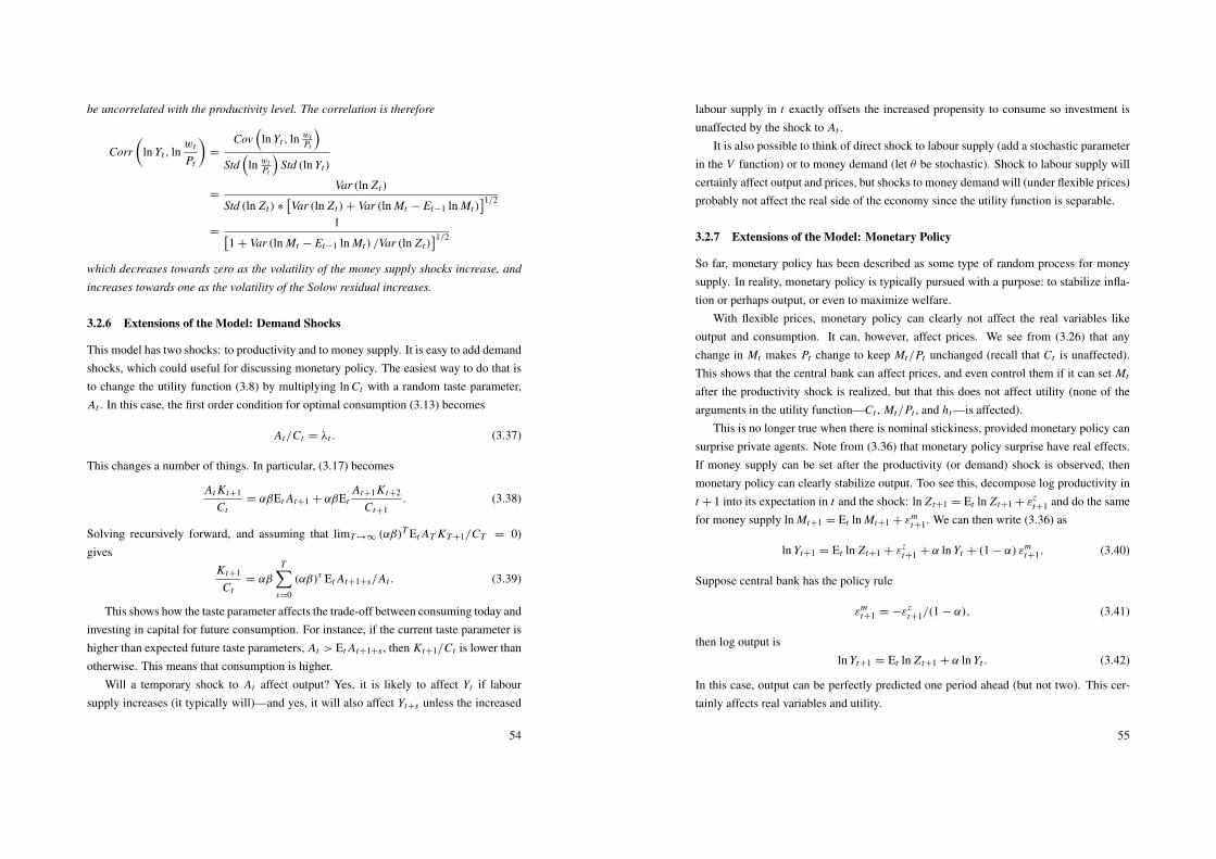
be uncorrelated with the productivity level. The correlation is therefore

Corr(

ln Yt , lnwt

Pt

)=

Cov(

ln Yt , ln wtPt

)Std

(ln wt

Pt

)Std (ln Yt)

=Var (ln Z t)

Std (ln Z t) ∗[Var (ln Z t)+ Var (ln Mt − Et−1 ln Mt)

]1/2=

1[1 + Var (ln Mt − Et−1 ln Mt) /Var (ln Z t)

]1/2which decreases towards zero as the volatility of the money supply shocks increase, and

increases towards one as the volatility of the Solow residual increases.

3.2.6 Extensions of the Model: Demand Shocks

This model has two shocks: to productivity and to money supply. It is easy to add demandshocks, which could useful for discussing monetary policy. The easiest way to do that isto change the utility function (3.8) by multiplying ln Ct with a random taste parameter,At . In this case, the first order condition for optimal consumption (3.13) becomes

At/Ct = λt . (3.37)

This changes a number of things. In particular, (3.17) becomes

At Kt+1

Ct= αβEt At+1 + αβEt

At+1Kt+2

Ct+1. (3.38)

Solving recursively forward, and assuming that limT →∞ (αβ)T Et AT KT +1/CT = 0)gives

Kt+1

Ct= αβ

T∑s=0

(αβ)s Et At+1+s/At . (3.39)

This shows how the taste parameter affects the trade-off between consuming today andinvesting in capital for future consumption. For instance, if the current taste parameter ishigher than expected future taste parameters, At > Et At+1+s , then Kt+1/Ct is lower thanotherwise. This means that consumption is higher.

Will a temporary shock to At affect output? Yes, it is likely to affect Yt if laboursupply increases (it typically will)—and yes, it will also affect Yt+s unless the increased

54

labour supply in t exactly offsets the increased propensity to consume so investment isunaffected by the shock to At .

It is also possible to think of direct shock to labour supply (add a stochastic parameterin the V function) or to money demand (let θ be stochastic). Shock to labour supply willcertainly affect output and prices, but shocks to money demand will (under flexible prices)probably not affect the real side of the economy since the utility function is separable.

3.2.7 Extensions of the Model: Monetary Policy

So far, monetary policy has been described as some type of random process for moneysupply. In reality, monetary policy is typically pursued with a purpose: to stabilize infla-tion or perhaps output, or even to maximize welfare.

With flexible prices, monetary policy can clearly not affect the real variables likeoutput and consumption. It can, however, affect prices. We see from (3.26) that anychange in Mt makes Pt change to keep Mt/Pt unchanged (recall that Ct is unaffected).This shows that the central bank can affect prices, and even control them if it can set Mt

after the productivity shock is realized, but that this does not affect utility (none of thearguments in the utility function—Ct , Mt/Pt , and ht—is affected).

This is no longer true when there is nominal stickiness, provided monetary policy cansurprise private agents. Note from (3.36) that monetary policy surprise have real effects.If money supply can be set after the productivity (or demand) shock is observed, thenmonetary policy can clearly stabilize output. Too see this, decompose log productivity int + 1 into its expectation in t and the shock: ln Z t+1 = Et ln Z t+1 + εz

t+1 and do the samefor money supply ln Mt+1 = Et ln Mt+1 + εm

t+1. We can then write (3.36) as

ln Yt+1 = Et ln Z t+1 + εzt+1 + α ln Yt + (1 − α) εm

t+1. (3.40)

Suppose central bank has the policy rule

εmt+1 = −εz

t+1/(1 − α), (3.41)

then log output isln Yt+1 = Et ln Z t+1 + α ln Yt . (3.42)

In this case, output can be perfectly predicted one period ahead (but not two). This cer-tainly affects real variables and utility.

55

3.3 “Money and the Business Cycle,” by Cooley and Hansen

Reference: Cooley and Hansen (1995).

3.3.1 Stylized Facts

Hodrick-Prescott filtered data (data minus a moving average: cycles longer than 8 yearsare virtually eliminated).

Variable (xt ): Corr(xt−2, ln GDPt ) Corr(xt , ln GDPt ) Corr(xt+2, ln GDPt )ln Yt 0.63 1 0.63ln M1/1 ln M1 0.41 0.33/− 0.12 0.12ln Velocity −0.08 0.37 0.33Nominal interest rate: −0.03 0.40 0.44Inflation: 0.01 0.34 0.44ln Price level: −0.72 −0.52 −0.17

Some facts:

1. Log money and log velocity (ln V = ln Y + ln P − ln M) are procyclical.

(a) Log money peaks before log output (Corr(ln M1t−1,ln Yt )>Corr(ln M1t ,ln Yt )> Corr(ln M1t+2,ln Yt )).

(b) Log velocity lags output.

2. The nominal interest rate (short) and inflation rate are also procyclical, but peaksafter output.

3. The log price level is counter cyclical.

3.3.2 Inflation Tax Model

This is a fairly standard real business cycle model, with some additional features. Astochastic money supply interacts with a cash-in-advance transaction technology to cre-ate some real effects of money supply shocks. The key equations are listed below. (Lower

56

case letters denote values for a representative household, whereas upper case letters de-note aggregates.)

Utility function : E0

∞∑t=0

β t [a ln c1t + (1 − a) ln c2t − γ ht ]

Real budget constraint : c1t + c2t + xt +mt+1

Pt=wt

Ptht + rtkt +

mt

Pt+

Tt

Pt.

Cash-in-advance constraint : Ptc1t = mt + Tt

Production function : Yt = ezt K θt H1−θ

t .

Capital accumulation : kt+1 = (1 − δ) kt + xt .

Government budget constraint : Tt = 1Mt+1.

Money supply : 1 ln Mt+1 = 0.491 ln Mt + ξt+1, ln ξt+1 ∼ N , known at t .

Log productivity : zt+1 = 0.95zt + εt+1, εt+1 ∼ N(

0, 4.9 × 10−5)

(Note: it should be Tt/Pt in the real budget constraint; there is a typo in the book.) Thenotation is: capital stock (K ), money stock (M), price level (P), wage rate (W ), hoursworked (H ), output (Y ), investment (X ), and productivity (z). Note that the notationdiffers somewhat from the model in Benassy (1995): the money stock held at the end ofperiod t is denoted Mt+1 (Mt in Benassy).

Private consumption consists of a “cash good,” c1t , and a “credit good,” c2t . Oneinterpretation of the trading sequence within a time period t is the following.

1. In the beginning of the period, the household carries over mt from t − 1, and getsTt is cash transfers from the government. Households also own all physical capital(kt ). Firms hold no cash or physical capital. The government finances the transfersby printing new money.

2. Firms rent capital and labor (the rent and wages are paid somewhat later in theperiod), and produce goods.

3. The household buys the cash good with the available cash, where the cash-in-advance restriction Ptc1t ≤ mt + Tt must hold. (The log-normal distribution ofthe money supply shock ξt means that the money stock can never decrease, whichis enough to ensure that the CIA constraint always binds: positive nominal interestrate with probability one.) Firms now hold mt + Tt in cash.

57

4. The household receives nominal factor payments wt ht + Ptrtkt from the firms (ex-hausts all profits), and buys credit goods (Ptc2t ) and investment goods (Pt xt ). Thefirms now hold no cash; households own the physical capital kt+1 = (1 − δ) kt +xt ,and the cash mt+1 = wt ht + Ptrtkt − Ptc2t − Pt xt .

5. In equilibrium, the money stock held by the households (mt+1) must equal moneysupply by the central bank (mt + Tt = Mt+1).

Calibration

The parameters in the production function, depreciation, Solow residual, and time pref-erence are chosen as in standard RBC models. The money supply process (for M1) isestimated with least squares. The a parameter is estimated from the first-order condition

C1t + C2t

C1t=

Pt (C1t + C2t)

PtC1t=

PtCt

mt=

1α

+1 − α

α*interest rate, (3.43)

where the paper uses the portion of M1 held by households as a proxy for mt (this differsfrom how they estimate the AR(1) for money supply, where they use all of M1). Iden-tifying a from the intercept, they get a = 0.85. (If they had identified α from the slopeinstead, then they would have got α = 0.9.)

To sum up, they use θ = 0.4, δ = 0.019, β = 0.989, γ = 2.53, and a = 0.84.Solving the ModelThe inflation tax means that the competitive solution will not coincide with the social

planners’s solution. The solution algorithm is therefore a based on the concept of recursivecompetitive equilibrium. Solving a quadratic approximation (in logs) of the model resultsin a set of linear decision rules in terms of the state of the economy. Productivity isstationary (|ρ| < 1), but the money supply is not, so prices will also be non-stationary. Itis therefore very convenient to “detrend” all nominal variables by dividing by Mt beforethe solution algorithm is applied.

Results

The model is simulated 100 times to generate artificial samples of 150 quarters, and thesimulated data is subsequently filtered with the Hodrick-Prescott filter. (Note: Tables 7.3-7.5 have the x(±s) columns in the reverse order compared with Tables 7.1-7.2, even if

58

this is not reflected by the headers: they should read (x(+5), ..., x, ..., x(−5).)Output is virtually neutral with respect to money supply shocks, even if the composi-

tion of aggregate demand is affected by the inflation tax. Intuition: 1 ln Mt ⇒expected

inflation⇒expensive to hold money so households substitute credit goods (and saving,that is future consumption) for cash goods.

The following table summarizes some properties of data and simulations (simulationresults in parentheses):

Variable (xt ): Corr(xt−2, ln G D Pt ) Corr(xt , ln G D Pt ) Corr(xt+2, ln G D Pt )ln Yt 0.63 (0.44) 1 (1) 0.63 (0.44)ln M1/1 ln M1 0.41 (?) 0.33/− 0.12 (?/0) 0.12 (?)ln Velocity −0.08 (0.48) 0.37 (0.95) 0.33 (0.35)Nominal interest rate: −0.03 (0.01) 0.40 (-0.01) 0.44 (0.01)Inflation: 0.01 (-0.06) 0.34 (-0.14) 0.44 (0.04)ln Price level: −0.72 (-0.06) −0.52 (-0.22) −0.17 (-0.16)

1. Correlation money growth and real variables very small (except for the correlationbetween money and the cash good which is very negative. In data, all correlationsbetween real variables and money growth are small.

2. Correlation output and interest rate/inflation is completely wrong.

3. Correlation output and velocity is much too strong.

4. For impulse response function, see Cooley Fig 7.6.

3.3.3 A Model with Nominal Wage Stickiness

The wage contract is based on the one-period ahead expectation of the marginal productof labor. The first order condition for profit maximization is

wt = (1 − θ) Ptezt

(Kt

Ht

)θ⇒ (3.44)

lnwt = ln (1 − θ)+ ln Pt + zt + θ (ln Kt − ln Ht) . (3.45)

It is assumed (ad hoc) that lnwt is set equal to the expectation of the right hand side of(3.45), conditional on the information in t − 1. Note that Kt is in the information set at

59

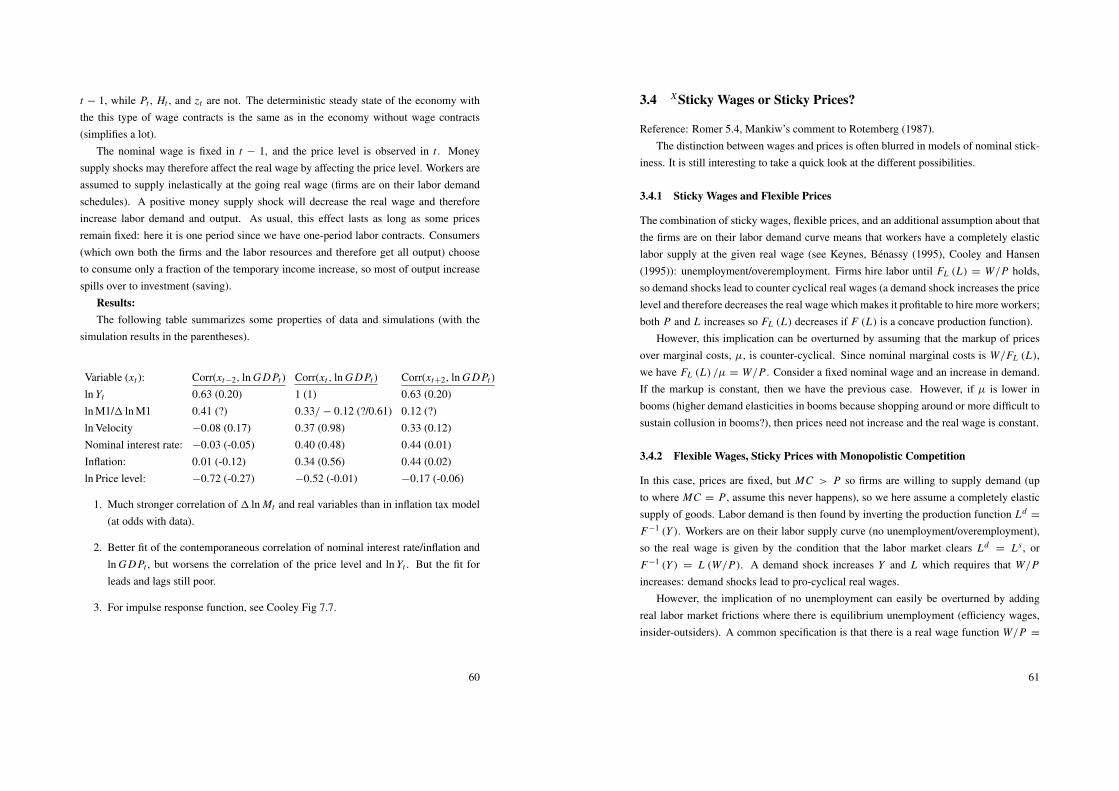
t − 1, while Pt , Ht , and zt are not. The deterministic steady state of the economy withthe this type of wage contracts is the same as in the economy without wage contracts(simplifies a lot).

The nominal wage is fixed in t − 1, and the price level is observed in t . Moneysupply shocks may therefore affect the real wage by affecting the price level. Workers areassumed to supply inelastically at the going real wage (firms are on their labor demandschedules). A positive money supply shock will decrease the real wage and thereforeincrease labor demand and output. As usual, this effect lasts as long as some pricesremain fixed: here it is one period since we have one-period labor contracts. Consumers(which own both the firms and the labor resources and therefore get all output) chooseto consume only a fraction of the temporary income increase, so most of output increasespills over to investment (saving).

Results:The following table summarizes some properties of data and simulations (with the

simulation results in the parentheses).

Variable (xt ): Corr(xt−2, ln G D Pt ) Corr(xt , ln G D Pt ) Corr(xt+2, ln G D Pt )ln Yt 0.63 (0.20) 1 (1) 0.63 (0.20)ln M1/1 ln M1 0.41 (?) 0.33/− 0.12 (?/0.61) 0.12 (?)ln Velocity −0.08 (0.17) 0.37 (0.98) 0.33 (0.12)Nominal interest rate: −0.03 (-0.05) 0.40 (0.48) 0.44 (0.01)Inflation: 0.01 (-0.12) 0.34 (0.56) 0.44 (0.02)ln Price level: −0.72 (-0.27) −0.52 (-0.01) −0.17 (-0.06)

1. Much stronger correlation of 1 ln Mt and real variables than in inflation tax model(at odds with data).

2. Better fit of the contemporaneous correlation of nominal interest rate/inflation andln G D Pt , but worsens the correlation of the price level and ln Yt . But the fit forleads and lags still poor.

3. For impulse response function, see Cooley Fig 7.7.

60

3.4 XSticky Wages or Sticky Prices?

Reference: Romer 5.4, Mankiw’s comment to Rotemberg (1987).The distinction between wages and prices is often blurred in models of nominal stick-

iness. It is still interesting to take a quick look at the different possibilities.

3.4.1 Sticky Wages and Flexible Prices

The combination of sticky wages, flexible prices, and an additional assumption about thatthe firms are on their labor demand curve means that workers have a completely elasticlabor supply at the given real wage (see Keynes, Benassy (1995), Cooley and Hansen(1995)): unemployment/overemployment. Firms hire labor until FL (L) = W/P holds,so demand shocks lead to counter cyclical real wages (a demand shock increases the pricelevel and therefore decreases the real wage which makes it profitable to hire more workers;both P and L increases so FL (L) decreases if F (L) is a concave production function).

However, this implication can be overturned by assuming that the markup of pricesover marginal costs, µ, is counter-cyclical. Since nominal marginal costs is W/FL (L),we have FL (L) /µ = W/P . Consider a fixed nominal wage and an increase in demand.If the markup is constant, then we have the previous case. However, if µ is lower inbooms (higher demand elasticities in booms because shopping around or more difficult tosustain collusion in booms?), then prices need not increase and the real wage is constant.

3.4.2 Flexible Wages, Sticky Prices with Monopolistic Competition

In this case, prices are fixed, but MC > P so firms are willing to supply demand (upto where MC = P , assume this never happens), so we here assume a completely elasticsupply of goods. Labor demand is then found by inverting the production function Ld

=

F−1 (Y ). Workers are on their labor supply curve (no unemployment/overemployment),so the real wage is given by the condition that the labor market clears Ld

= Ls , orF−1 (Y ) = L (W/P). A demand shock increases Y and L which requires that W/P

increases: demand shocks lead to pro-cyclical real wages.However, the implication of no unemployment can easily be overturned by adding

real labor market frictions where there is equilibrium unemployment (efficiency wages,insider-outsiders). A common specification is that there is a real wage function W/P =

61

w (L)which together with labor demand determine a real wage rate, where workers wouldbe willing to supply more labor.

Bibliography



Cooley, T. F., and G. D. Hansen, 1995, “Money and the Business Cycle,” in Thomas F.Cooley (ed.), Frontiers of Business Cycle Research, Princeton University Press, Prince-ton, New Jersey.

Long, J. B., and C. I. Plosser, 1983, “Real Business Cycles,” Journal of Political Economy,91, 39–69.



Rotemberg, J. J., 1987, “New Keynesian Microfoundations,” in Stanley Fischer (ed.),NBER Macroeconomics Annual . pp. 69–104, NBER.


62

4 Money in Models of Monopolistic Competition

4.1 Monopolistic Competition

Reference: Walsh (1998) 5.3 (See also Romer (1996) 6.6, Blanchard and Fischer (1989)8.1, and Obstfeldt and Rogoff (1996) 10.1)

Background: Monopolistic competition do not, in itself, lead to a role for monetarypolicy—nominal stickiness does. Monopolistic competition is only a starting point fordiscussing price setting behaviour.

4.1.1 Producers of the Final Good

The final good (the good that enters the utility function of agents) is produced by compet-itive firms. The production function is a CES function (with constant returns to scale) ofa continuum of intermediate goods Y (i), indexed by i ∈ [0, 1]

Yt =

(∫ 1

0Y (i)q di

) 1q

, 0 < q < 1. (4.1)

Example 26 (CES production function with two inputs.) Consider the CES production

function

y =(xq

1 + xq2

)1/q.

We get a linear production function, y = x1+x2, if q = 1; a Leontief production function,

, y = min (x1, x2), if q = −∞; and a Cobb-Douglas production function, y = x1/21 x1/2

2 ,

if q = 0.

The price of Y (i) is P (i). Profits of a firm in the final good sector are

π = PY −

∫ 1

0P (i) Y (i) di

= P

(∫ 1

0Y (i)q di

) 1q

−

∫ 1

0P (i) Y (i) di. (4.2)

63

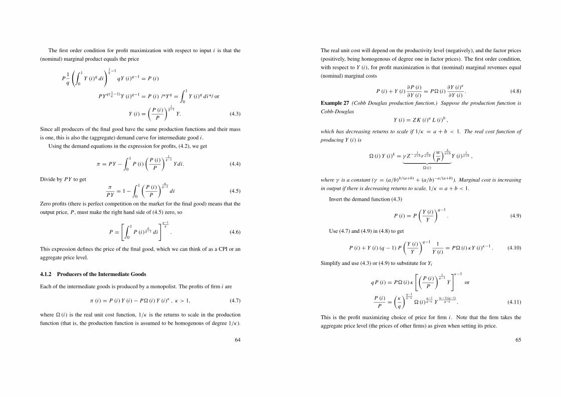
The first order condition for profit maximization with respect to input i is that the(nominal) marginal product equals the price

P1q

(∫ 1

0Y (i)q di

) 1q −1

qY (i)q−1= P (i)

PY q( 1q −1)Y (i)q−1

= P (i) /*Y q=

∫ 1

0Y (i)q di*/ or

Y (i) =

(P (i)

P

) 1q−1

Y. (4.3)

Since all producers of the final good have the same production functions and their massis one, this is also the (aggregate) demand curve for intermediate good i .

Using the demand equations in the expression for profits, (4.2), we get

π = PY −

∫ 1

0P (i)

(P (i)

P

) 1q−1

Y di. (4.4)

Divide by PY to getπ

PY= 1 −

∫ 1

0

(P (i)

P

) qq−1

di (4.5)

Zero profits (there is perfect competition on the market for the final good) means that theoutput price, P , must make the right hand side of (4.5) zero, so

P =

[∫ 1

0P (i)

qq−1 di

] q−1q

. (4.6)

This expression defines the price of the final good, which we can think of as a CPI or anaggregate price level.

4.1.2 Producers of the Intermediate Goods

Each of the intermediate goods is produced by a monopolist. The profits of firm i are

π (i) = P (i) Y (i)− P�(i) Y (i)κ , κ > 1, (4.7)

where �(i) is the real unit cost function, 1/κ is the returns to scale in the productionfunction (that is, the production function is assumed to be homogenous of degree 1/κ).

64

The real unit cost will depend on the productivity level (negatively), and the factor prices(positively, being homogenous of degree one in factor prices). The first order condition,with respect to Y (i), for profit maximization is that (nominal) marginal revenues equal(nominal) marginal costs

P (i)+ Y (i)∂P (i)∂Y (i)

= P�(i)∂Y (i)κ

∂Y (i). (4.8)

Example 27 (Cobb Douglas production function.) Suppose the production function is

Cobb-Douglas

Y (i) = Z K (i)a L (i)b ,

which has decreasing returns to scale if 1/κ = a + b < 1. The real cost function of

producing Y (i) is

�(i) Y (i)k = γ Z−1

a+b ra

a+b

(wP

) ba+b︸︷︷︸

�(i)

Y (i)1

a+b ,

where γ is a constant (γ = (a/b)b/(a+b)+ (a/b)−a/(a+b)). Marginal cost is increasing

in output if there is decreasing returns to scale, 1/κ = a + b < 1.

Invert the demand function (4.3)

P (i) = P(

Y (i)Y

)q−1

. (4.9)

Use (4.7) and (4.9) in (4.8) to get

P (i)+ Y (i) (q − 1) P(

Y (i)Y

)q−1 1Y (i)

= P�(i) κY (i)κ−1 . (4.10)

Simplify and use (4.3) or (4.9) to substitute for Yi

q P (i) = P�(i) κ

[(P (i)

P

) 1q−1

Y

]κ−1

or

P (i)P

=

(κ

q

) q−1q−κ

�(i)q−1q−κ Y

(κ−1)(q−1)q−κ . (4.11)

This is the profit maximizing choice of price for firm i . Note that the firm takes theaggregate price level (the prices of other firms) as given when setting its price.

65

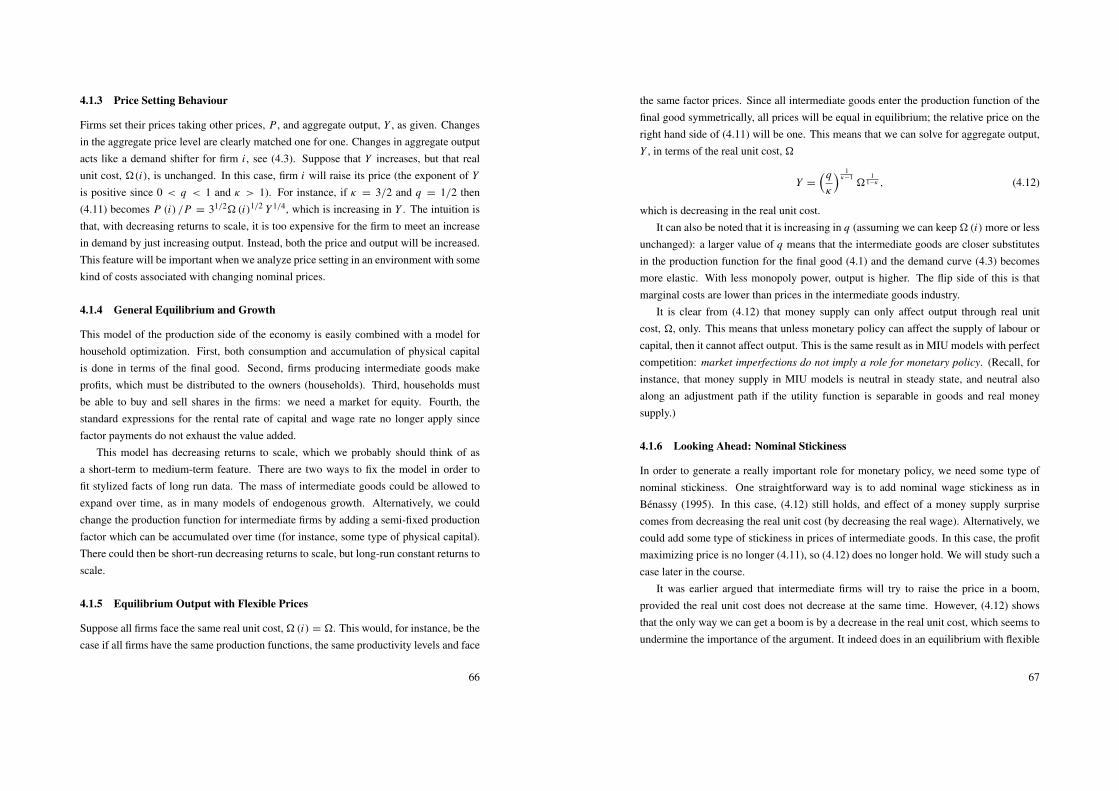
4.1.3 Price Setting Behaviour

Firms set their prices taking other prices, P , and aggregate output, Y , as given. Changesin the aggregate price level are clearly matched one for one. Changes in aggregate outputacts like a demand shifter for firm i , see (4.3). Suppose that Y increases, but that realunit cost, �(i), is unchanged. In this case, firm i will raise its price (the exponent of Y

is positive since 0 < q < 1 and κ > 1). For instance, if κ = 3/2 and q = 1/2 then(4.11) becomes P (i) /P = 31/2�(i)1/2 Y 1/4, which is increasing in Y . The intuition isthat, with decreasing returns to scale, it is too expensive for the firm to meet an increasein demand by just increasing output. Instead, both the price and output will be increased.This feature will be important when we analyze price setting in an environment with somekind of costs associated with changing nominal prices.

4.1.4 General Equilibrium and Growth

This model of the production side of the economy is easily combined with a model forhousehold optimization. First, both consumption and accumulation of physical capitalis done in terms of the final good. Second, firms producing intermediate goods makeprofits, which must be distributed to the owners (households). Third, households mustbe able to buy and sell shares in the firms: we need a market for equity. Fourth, thestandard expressions for the rental rate of capital and wage rate no longer apply sincefactor payments do not exhaust the value added.

This model has decreasing returns to scale, which we probably should think of asa short-term to medium-term feature. There are two ways to fix the model in order tofit stylized facts of long run data. The mass of intermediate goods could be allowed toexpand over time, as in many models of endogenous growth. Alternatively, we couldchange the production function for intermediate firms by adding a semi-fixed productionfactor which can be accumulated over time (for instance, some type of physical capital).There could then be short-run decreasing returns to scale, but long-run constant returns toscale.

4.1.5 Equilibrium Output with Flexible Prices

Suppose all firms face the same real unit cost,�(i) = �. This would, for instance, be thecase if all firms have the same production functions, the same productivity levels and face

66

the same factor prices. Since all intermediate goods enter the production function of thefinal good symmetrically, all prices will be equal in equilibrium; the relative price on theright hand side of (4.11) will be one. This means that we can solve for aggregate output,Y , in terms of the real unit cost, �

Y =

(qκ

) 1κ−1�

11−κ , (4.12)

which is decreasing in the real unit cost.It can also be noted that it is increasing in q (assuming we can keep�(i)more or less

unchanged): a larger value of q means that the intermediate goods are closer substitutesin the production function for the final good (4.1) and the demand curve (4.3) becomesmore elastic. With less monopoly power, output is higher. The flip side of this is thatmarginal costs are lower than prices in the intermediate goods industry.

It is clear from (4.12) that money supply can only affect output through real unitcost, �, only. This means that unless monetary policy can affect the supply of labour orcapital, then it cannot affect output. This is the same result as in MIU models with perfectcompetition: market imperfections do not imply a role for monetary policy. (Recall, forinstance, that money supply in MIU models is neutral in steady state, and neutral alsoalong an adjustment path if the utility function is separable in goods and real moneysupply.)

4.1.6 Looking Ahead: Nominal Stickiness

In order to generate a really important role for monetary policy, we need some type ofnominal stickiness. One straightforward way is to add nominal wage stickiness as inBenassy (1995). In this case, (4.12) still holds, and effect of a money supply surprisecomes from decreasing the real unit cost (by decreasing the real wage). Alternatively, wecould add some type of stickiness in prices of intermediate goods. In this case, the profitmaximizing price is no longer (4.11), so (4.12) does no longer hold. We will study such acase later in the course.

It was earlier argued that intermediate firms will try to raise the price in a boom,provided the real unit cost does not decrease at the same time. However, (4.12) showsthat the only way we can get a boom is by a decrease in the real unit cost, which seems toundermine the importance of the argument. It indeed does in an equilibrium with flexible

67

prices, but it need not do so in an equilibrium with (some) sticky prices. For instance,when (some) prices are sticky and quantities are demand determined (for some reason,firms post prices in advance and agree to supply whatever is demanded at the price), thenthose firm that do not have sticky prices will increase them in booms.

Bibliography






68

5 Money and Price Setting

Main references: Romer (1996) (Romer), Blanchard and Fischer (1989) (BF), Obstfeldtand Rogoff (1996) (OR), and Walsh (1998)

5.1 Dynamic Models of Sticky Prices

References: BF. 8.2, Romer 6.7, Rotemberg (1987).This section deals with the effect of price rigidities in dynamic models. Prices are set

in advance and firms are assumed to supply whatever demand happens to be (which is rea-sonable only as long as demand shocks do not force marginal costs above the price). Thisclearly assumes that firms can expand production, for instance, by hiring more labour, sothere must be a fairly elastic factor supply. If factor supply is not particularly elastic, thenmarginal costs will increase rapidly so the assumption that marginal cost is always belowthe price becomes implausible.

Aggregate demand shocks (or money supply) will usually have real effects whenprices adjust slowly. This is certainly the case when prices are changed with prespeci-fied intervals (time-dependent rules), and the main issue is instead how long the effectslast. It is typically also the case when prices are changed when the old prices are too farfrom the frictionless optimum (state dependent rules).

In general, we would like to find a reasonable model which can explain both whyaverage prices seem to adjust gradually to monetary expansions and why price changesof individual firms appear to be “lumpy.” This is hard.

5.1.1 Quadratic Costs of Price-Adjustment

Reference: Rotemberg (1982a), Rotemberg (1982b), and Walsh 5.5.Firm i is a monopolist on its market and sets the log price, pi t , to maximize the value

of the firm: the expected discounted sum of profits. If there were no costs of adjustingthis price, then the price would be equal to some value, p∗

i t , which we call the flex priceoptimum.

69

With costs of adjusting the price we formulate the maximization problem in two steps.First, find the flex price optimum, p∗

i t . Second, minimize the loss from not being at p∗

i t

and from incurring adjustment costs. For the moment, we will take the time series processof p∗

i t as given and focus on the second part of the maximization problem. To make anyprogress, we also approximate the objective function in the second step by a quadraticfunction

min{pi t+s}

∞

s=0

Et

∞∑s=0

βs[(

pi t+s − p∗

i t+s)2

+ c (pi t+s − pi t+s−1)2]

or (5.1)

min{pi t+s}

∞

s=0

{(pi t − p∗

i t)2

+ c (pi t − pi t−1)2+ βEt

(pi t+1 − p∗

i t+1)2

+ βcEt (pi t+1 − pi t)2+ ...

}.

The first order condition with respect to pi t is

pi t − p∗

i t + c (pi t − pi t−1)− βcEt (pi t+1 − pi t) = 0 or (5.2)

βEt1pi t+1 +1c

(p∗

i t − pi t)

= 1pi t . (5.3)

There is no lumpiness in individual price changes. Since both deviations from the p∗

i t andprices changes are much more costly when they are large (the loss function is quadratic),the optimal policy will be to converge to p∗

i t by taking many small steps rather than afew large. In a symmetric equilibrium pi t = pt and p∗

i t = p∗t . It can also be noted

that situations with a high surprise inflation will lead to a higher p∗

i t − pi t , so the priceadjustment is then faster.

The smooth individual price changes carry over to the average prices, since all firmsare similar. Let pi t = pt and p∗

i t = p∗t be the common prices and write (5.3) as

1pt = βEt1pt+1 +1c

(p∗

t − pt). (5.4)

Special Case: No Adjustment Cost (c = 0)

If c = 0, then (5.2) shows that pi t = p∗

i t , so the firm will always set its actual price equalto the unrestricted optimal price (quite obvious since the price is then unrestricted).

5.1.2 Calvo’s Model

Reference: Rotemberg (1987) and Walsh 5.5.

70

In contrast to the model with quadratic adjustment costs, this model has lumpy indi-vidual price changes—but it gives the same evolution of the average price level (shownbelow).

Prices are changed at exogenous random points in time only. The fraction q of thefirms are allowed to set a new price in a period, and the fraction 1 − q must keep their oldprice. As in the model with quadratic adjustment costs, the model is set up in two steps.First, find the flex price optimum, p∗

i t . Second, minimize the loss from not being at p∗

i t ,taking into account the firm only gets a time to change its price at random occasions.

Let p∗

i t+s be the flex price optimum of firm i in period t + s, and pi t the actual priceset in t (and perhaps still valid in future periods if no opportunity to change the price hasoccurred). The frequency of price changes is, unrealistically, assumed to be constant.

Suppose firm i gets to change its price in t . The minimization problem in t is to choosethe price, pi t , to minimize the expected discounted loss of being away from the optimalprice. The loss function is once again approximated by a quadratic function

L t = Et

∞∑s=0

βs ( pt+s − p∗

i t+s)2, (5.5)

where pt+s denotes actual price in t + s, which might have been set in the same or someearlier period.

This loss function is potentially problematic since pt+s has a mixture (both discreteand continuous parts to it) distribution, which can make it complicated to calculate theexpected value (note that pt+s and p∗

i t+s are likely to be correlated in a complicated way).However, we can simplify the problem by noting that all we care about are the terms thatinvolve pt+s = pi t . First, note that the next time the firm will get to change its price isin the random time t + τ1, the second time in t + τ2, and so forth. The probability that itdoes not get to change the price in t + 1 is 1 − q , that it does not get to change in eithert + 1 or in t + 2 is (1 − q)2, and so forth. This means that Pr( pt+s = pi t) = (1 − q)s .Second, note that Et( pt+s − p∗

i t+s)2

=∫�( pt+s − p∗

i t+s)2d F( pt+s, p∗

i t+s), where F isthe joint distribution function and

∫�

be understood as a Stieltjes integral over �, whichis the space of values of the pair { pt+s, p∗

i t+s}. We can split up � into two subsets: onewhere pt+s = pi t and the rest. Clearly, only the first subset matters for the first ordercondition with respect to pi t . This subset has the probability (1 − q)s and p∗

i t+s has somedistribution (only the first moment will be important).

71

We therefore rewrite the loss function (5.5) as

L t =

∞∑s=0

βs (1 − q)s Et(

pi t − p∗

i t+s)2

+ terms not involving pi t , (5.6)

where pi t is the price set in t (and still in effect in t + s with probability (1 − q)s). (Analternative, and more careful, derivation is given in Appendix B.)

The first order condition with respect to pi t is

∞∑s=0

βs (1 − q)s(

pi t − Et p∗

i t+s)

= 0. (5.7)

Since∑

∞

s=0 βs (1 − q)s = 1/[1 − β (1 − q)], we get

pi t = [1 − β (1 − q)]∞∑

s=0

βs (1 − q)s Et p∗

i t+s (5.8)

= [1 − β (1 − q)] p∗

i t + [1 − β (1 − q)]β (1 − q)∞∑

s=0

βs (1 − q)s Et p∗

i t+1+s . (5.9)

This can be rewritten as a forward looking difference equation in pi t by noting that thelast term in (5.9) equals β (1 − q)Et pi t+1, see (5.8). (This is the price they would set int + 1 if they get to change the price then.) This gives

pi t = [1 − β (1 − q)] p∗

i t + β (1 − q)Et pi t+1. (5.10)

If all firms are similar, then pi t and p∗

i t are the same for all firms. The aggregateprice level is the weighted average of those who get to change the price and those whodid not. (This can be seen as an approximation to a true CPI. For instance, if the utilityfunction/production function for the final good is CES, then the exact CPI is also a CESfunction.) The latter have, on average, a price equal to the price level in t − 1 (since thedraws are independent over time). The average price level is therefore

pt = qpi t + (1 − q) pt−1, so (5.11)

pi t =1q

pt −1 − q

qpt−1 (if q > 0). (5.12)

Use this to substitute for pi t and pi t+1 in (5.10) and let all firms have the same flex price,

72

p∗

i t = p∗t(

1q

pt −1 − q

qpt−1

)= [1 − β (1 − q)] p∗

t + β (1 − q)Et

(1q

pt+1 −1 − q

qpt

), or

(5.13)

1pt = βEt1pt+1 +q

1 − q[1 − β (1 − q)]

(p∗

t − pt). (5.14)

This is of the same form as (5.4), but where the coefficients have different interpretations.

Special Case: Flexible Prices (q = 1)

If q = 1, so all firms get to change their prices in every period, then (5.10) becomes

pi t = p∗

i t , (5.15)

so prices are set equal to the flex price optimal.

Average Time between Price Changes

Price changes follows a Poisson process, so time to a price change has an exponentialdistribution.(The exponential distribution is q exp (−qτ) for τ > 0, with Eτ = 1/q andVar(τ ) = 1/q2.)

5.1.3 Other Ways to Model Price Stickiness

It is straightforward (but a bit tedious) to model multi-period price contracts. It could,for instance, be a case where half the firms set prices for two periods in every odd timeperiod, and the other half in every even period (staggered price setting).

The Fischer model allows the contract to stipulate different (but predetermined) pricesfor the different subperiods of the contract. The Taylor model is similar, but has the sameprice for all subperiods (fixed prices), which gives more price inertia.

5.1.4 Price Setting in a Model with Monopolistic Competition

What is the unrestricted optimal price, p∗

i t , which plays such an important role in theprevious model? A typical formulation is that it represents a monopolist’s price in a flex-price equilibrium. That price is typically an increasing function of aggregate demand and

73

a decreasing function of the productivity level. In logs, we write

p∗

t = pt + φyt + εt , (5.16)

where εt is interpreted as the negative of a productivity shock (negative “supply shock”).Note that φ > 0. It is typically increasing in slope of the marginal cost curve (the degreeof decreasing returns to scale) and decreasing in the elasticity of substitution betweengoods in consumer preferences. In most models, we need an upward sloping marginalcost curve to get φ > 0, which could be motivated by some fixed factors of production.If these fixed factors are not completely fixed, but can be accumulated over time, thenthe problem becomes more complicated (dynamic) and (5.16) can only be interpreted asan approximation that might be valid for short to medium run horizons (a business cycle,say).

Using (5.16) in (5.4) gives

1pt = βEt1pt+1 +1c(φyt + εt) . (5.17)

Similarly, using (5.16), in (5.13) gives

1pt = βEt1pt+1 +q

1 − q[1 − β (1 − q)] (φyt + εt) . (5.18)

We write both these equations as

1pt = βEt1pt+1 + δ (φyt + εt) , (5.19)

which can be thought of as an expectations-augmented Phillips curve. It is in an sensesimilar to the Keynesian AS curve, which has positive relation between output and theprice level.

Recursion forward gives

1pt = δ

∞∑s=0

βsEt (φyt+s + εt+s) , (5.20)

provided lims→∞ βs+1Et1pt+s = 0. Note that Et yt+s has a large effect on inflation is φ ishigh (strong decreasing returns to scale and/or strong market power), and Et (φyt+s + εt+s)

has a large effect if δ is high (small c in (5.17) or large q in (5.19)).

74

As in any Phillips curve, it appears as if inflation is a real phenomenon! This is quitethe opposite to the Cagan model, where it is assumed that both output and the real interestrate are constant. This suggests that this model of price setting is certainly not suitable forunderstanding a permanent change in the money supply trend. It is not plausible that themodel parameters, for instance q and c, would remain unchanged in such a case.

5.1.5 Closing the Model: The Demand Side

We need a model for yt to illustrate how this price setting works. Suppose we havemacro model with money in the utility function/cash in advance, optimizing households,imperfect competition with (at least temporarily) decreasing returns to scale, and costs ofchanging nominal prices. We also add the assumption that firms with sticky prices agreeto sell any quantity demanded at the prevailing price.

In this setting, (5.19) describes how firms set prices. The rest of the model would besomething like the following. Money demand is

mt − pt = ψyt − ωit . (5.21)

The Euler equation for consumption is C−γt = (1 + rt+1)EtC

−γ

t+1, which is approximatelyequal to the following (in logs)

−γ ct = −γEtct+1 + rt+1 or rt+1 = γ (Etct+1 − ct) , (5.22)

where rt+1 is the real interest rate. If assume that consumption is approximately propor-tional to output, then (5.22) can be written

rt+1 = γ (Et yt+1 − yt)+ constant. (5.23)

The Fisher equation isit = Et (pt+1 − pt)+ rt+1. (5.24)

Finally, we have to add an assumption about what the central bank uses as its instrument:mt or it . This is the whole model. We could clearly add more features, for instance, alabour supply decision (must be elastic to let the firms expand output), but we disregardthat in order to keep the model as simple as possible.

Consider the case when the central bank sets mt . When money is interest rate elastic,

75

ω 6= 0, then (5.19) and (5.21) are no longer sufficient to close the model, since thenominal interest rate remains to be determined. From the Fisher equation (5.24) we seethat determining the nominal interest rate requires both inflation (already captured by(5.19)) and the real interest rate. We therefore need a model of the real interest rate, forinstance, (5.23), to close the model. In contrast, when ω = 0, then we do not need amodel of the real interest rate in order to solve for the equilibrium price and output. Ofcourse, we can always plug in the equilibrium process for yt in (5.23) to calculate theimplied real interest rate, but we do not have to.

Now, consider the case when the central bank sets it . In this case, we do not need themoney demand equation (5.21) for determining the price and output. Instead, we combine(5.19) with (5.23) and (5.24) to give us a model in terms of the price, output, real interestrate, and the nominal interest rate (set by central bank). Of course, we can always plug inthe equilibrium values in (5.21) to calculate money demand, but we do not have to.

5.1.6 Example: Calvo Model in a Very Simple Macro Model

For simplicity, assume that the quantity equation holds. In logs we have

mt = pt + yt . (5.25)

This can be taken to represent aggregate demand. Aggregate supply is represented bythe price setting rule, and it is assumed that firms supply whatever the market demandsat the going price: output is demand determined. In traditional monetarist models, thequantity equation is aggregate demand, without much discussion of where it comes from.In a Keynesian model, the quantity equation would be an approximation to the KeynesianAD curve (the combination of the IS and LM curves which traces out the relation betweenoutput and prices). Both these interpretations assume a negative relation between the pricelevel and output. In some modern dynamic general equilibrium models, the quantityequation can be shown to be the money demand equation (see, for instance, Benassy(1995)).

We now use this very simple model of “demand” to illustrate some properties of the

76

sticky price model. Substitute for yt in (5.19) by using (5.25)

1pt = βEt1pt+1 + δφ (mt − pt)+ δεt

−pt−1 + pt (1 + β + δφ)− βEt pt+1 = δ (φmt + εt) . (5.26)

This is a second-order expectational difference equation, which can be solved with avariety of methods. The perhaps most straightforward one is to specify a time-seriesprocess for the exogenous driving process, and transform the system to a vector first-ordersystem and then use a decomposition of the resulting matrix to decouple the variables inthose that are predetermined in t (typically the exogenous variables and values determinedin previous periods like the capital stock and lagged variables) and those that can jumpin t in response to changes in expectations about future values (typically asset prices andanything else that depend on expected future values).

A trivial step is to note that (5.26) can be rewritten

Et pt+1 = −1β

pt−1 + pt1 + β + δφ

β−δ

β(φmt + εt) . (5.27)

Suppose εt = 0 and that mt is an AR(1)

mt = ρmt−1 + εmt . (5.28)

We can then write the model on state space form as mt+1

pt

Et pt+1

=

ρ 0 00 0 1−δβφ −

1β

1+β+δφβ

mt

pt−1

pt

+

εmt+1

00

. (5.29)

Some impulse response functions (dynamic simulations obtained from setting εmt = 1in t = 0 but zero in all other periods) are shown in Figure 5.1. In Figure 5.1.a, price ad-justment is fairly slow (many prices are fixed in spite of an increase in nominal demand),so a monetary shock leads to a relatively large effect on output: money is far from neutral.In Figure 5.1.b, price adjustment is much faster (the rate at which an occasion to changethe price arrives is much higher), so the monetary shock has almost no effect on output:money is almost neutral. In Figure 5.1.c also has fat price adjustment, but now becauseφ is high (quickly decreasing returns to scale or strong monopoly power), which makes ittoo costly for firms to keep their old prices.

77

−2 0 2 4 6 8

0

0.5

1a. Baseline model

period

money

price

output

−2 0 2 4 6 8

0

0.5

1

b. Frequent price adjustments, q=0.99

period

−2 0 2 4 6 8

0

0.5

1

c. Prices sensitive to demand, φ=2

period

Calvo model, response to money supply shock

Parameter values (base line):

ρ=0.95, φ=3/7, q=0.875, β=0.96

Figure 5.1: Impulse responses in the Calvo model

5.1.7 The Calvo Model and the “Natural Rate Hypothesis”

Reference: Walsh 5.5.The “natural rate hypothesis” states that the mean of output cannot be affected by any

monetary policy. Suppose the central bank can change the inflation rate by changing itspolicy instrument. Take the unconditional expectation of the Calvo model (5.19) and useiterated expectations and Eεt = 0 to get

Eyt =E1pt − βE1pt+1

δφ. (5.30)

If β = 1 (β < 1), and inflation is a stationary series so E1pt = E1pt+1, then thismeans that inflation cannot (can) affect average output. Irrespective of whether β = 1 ornot, a drifting inflation rate (E1pt 6=E1pt+1) can certainly affect average output.

This should probably be regarded as an artifact of the Calvo model. It puts restrictions

78

on which type of policy experiments which are meaningful to analyze with the help ofthis model: we should probably only use this model for policy changes which keeps theaverage inflation rate unchanged. In many applications, the Phillips equation is assumedto refer to detrended output (as a measure of the business cycle). The main reason isthat the Phillips effect is typically only relevant for as long as the production functionhas decreasing returns to scale, see the discussion of (5.16). Since detrended output perdefinition has a zero mean the kind of experiments that changes Eyt must be ruled out.

5.1.8 Empirical Illustration

• Relation between output and unemployment: Okun’s law, 1 ln Yt = 31ut .

• Phillips curve unstable, in particular if not accounting for Etπt+1. (Burda andWyplosz (1997) Figs. 12.4 and 12.6)

• OR Box 10.2 (substantial evidence of imperfect competition from micro data of 50US industries)

• OR Box 10.1 (12-18 months between price changes on selected items in US mailcatalogues)

• Rotemberg (1982b) finds that for Germany the average time between price changeswas 4 quarters. It must therefore be the case that 1/q = 4, so q = 1/4. He reportseven lower numbers for the US.

• Roberts (1995) estimates

1pt−Et1pt+1 = co+γ yt+c11(log real oil pricet

)+c21

(log real oil pricet−1

)+εt ,

where 1pt is measured by the percentage increase December to December in CPI,yt GDP detrended with a deterministic trend (time and time squared), and Et1pt+1

is approximated by inflation expectation surveys. The sample is annual and covers1949-1990. The results are γ ≈ 0.3. If we use this together with q = 1/4 (fromRotemberg (1982b)) and β = 1 in (5.18), we get φ ≈ 3.6, so a one percent increasein aggregate demand drives up the desired relative price of a monopolist with 3.6percent.

79

5.2 Aggregation of One-Sided Ss Rule: A Counter-Example to1M →

1Y ∗

Reference: BF. 408-414, Romer 273-276.Basic point: individual price stickiness does not necessarily imply aggregate price

stickiness.If there where no adjustment costs the optimal nominal price of a firm i is

p∗

i t = mt . (5.31)

Assume that mt is non-decreasing, so

mt ≥ mt−1t , (5.32)

which makes the frictionless optimum p∗

i t drift upwards. Suppose the actual price set bythe firm is pi t , and that there is a menu cost for changing the price. It can be shown that aone-sided Ss rule is optimal

pi t =

{pi t−1t if pi t−1t > p∗

i t − S, S > 0p∗

i t − s else, s < 0., (5.33)

where S and s depend on the drift and the menu cost.This rule implies that the nominal price is unchanged as long as the frictionless op-

timum p∗ is not much larger that the actual price. At a price change, the actual price isset somewhat higher than the frictionless price pi t = p∗

i t − s, s < 0, in expectation ofincreases in p∗

i (mt drifts upwards all the time).Consider an example. We start with p0 = p∗

0 , and then p∗t increases until it reaches

p0 + S in period τ . At that time the actual price is changed to

pτ = p∗

τ − s

= p0 + S − s /*price is changed when p∗

τ = p0 + S*/

> p0 + S /*since s < 0*/ (5.34)

The deviation p∗− p moves within the band [s, S].

In general, this type of setup implies a uniform distribution of p∗− p over the band

80

[s, S] with pdf

f(

p∗− p

)=

1S − s

. (5.35)

What is the effect on real balances of an infinitesimal increase in money stock dm.For all firms which have p∗

− p ∈ [s, S), that is, below the point which triggers a pricechange, all firms are simply shifted up in parallel. For all firms which are moved to thetrigger point (p∗

− p = S), we see an immediate adjustment of the price to, so p∗− p = s.

These two movements completely offsets each other, so the average p∗− p is unchanged.

If supply depends on real balances, then output is unaffected by the change in moneysupply.

Critical assumptions and discussion. The initial distribution is uniform and shocksare small. The general contribution of the model is to highlight the importance of the dis-tribution of price/frictionless price. One could envision a situation where a large fractionof firms are close to adjusting there price upwards. I small (but not infinitesimal) changein money supply can then trigger a disproportionate jump in the average price level, sothat a monetary expansion leads to a recession.

A Summary of Solution Method for Linear RE Models

A.1 Summary

The model is [x1t+1

Et x2t+1

]= A

[x1t

x2t

]+

[εt+1

0

], (A.1)

where x1t is an n1 × 1 vector of predetermined variables, x2t is an n2 vector of “forwardlooking” variables, and εt is a white noise process. All dynamics of the exogenous pro-cesses have been placed in x1t . A necessary condition for a saddle path equilibrium is thatA has as many unstable roots (inside unit circle) as there are elements in x1t .

Decompose A asA = Z T Z−1, (A.2)

where T is (at least) upper block diagonal. Note that we require Z to be invertible. Insome cases we could let T be a diagonal matrix with eigenvalues along the principaldiagonal and with the corresponding eigenvectors in the columns of Z (if the eigenvectors

81

are linearly independent).This decomposition should be reordered so that the blocks corresponding to the stable

eigenvalues (in or on the unit circle) comes first. Partition conformably with the stableand unstable roots

T =

[Tθθ Tθδ0 Tδδ

]and Z =

[Zkθ Zkδ

Zλθ Zλδ

]. (A.3)

The solution can then be shown to be

x1t+1 = ZkθTθθ Z−1kθ x1t + εt+1 (A.4)

x2t = Zλθ Z−1kθ x1t . (A.5)

A.2 Special Case: Scalar Second Order Equation

Reference: Romer 6.8, BF Appendix to chap 5, Hamilton (1994) 2.3.Consider the homogenous scalar second order difference equation

xt+1 − axt − bxt−1 = 0. (A.6)

We can write the difference equation as a system of first order equations as in (A.1)(with εt = 0 for all t) [

xt

xt+1

]=

[0 1b a

][xt−1

xt

]. (A.7)

The matrix can be decomposed in terms of eigenvalues and eigenvectors. It can be shownthat the decomposition is[

0 1b a

]=

[−λ2/b −λ1/b

1 1

][λ1 00 λ2

][−λ2/b −λ1/b

1 1

]−1

, (A.8)

where [λ1

λ2

]=

[12a −

12

√a2 + 4b

12a +

12

√a2 + 4b

], (A.9)

and where the eigenvalues satisfy

a = λ1 + λ2 and b = −λ1λ2. (A.10)

82

We assume that a and b are such that |λ1| < 1 but |λ2| > 1.

Example 28 a = 1.1 and b = 0.3 gives λ1 ≈ −0.23 and λ2 ≈ 1.323.

In this case, (A.4) givesxt = λ1xt−1, (A.11)

since Zkθ = −λ2/b and Tθθ = λ1.It is straightforward to show that (A.11) satisfies (A.6). From (A.11), xt = λ1xt−1 ,

so xt+1 = λ1xt = λ21xt−1, so (A.6) becomes

λ21 − aλ1 − b, (A.12)

which should be zero. Substituting for a and b from (A.10) immediately shows that thisis the case.

We now generalize the scalar difference equation to

Et xt+1 − axt − bxt−1 = Et zt , (A.13)

where zt is some exogenous process.It can then be shown that the solution is

xt = λ1xt−1 −1λ2

∞∑s=0

(1λ2

)s

Et zt+s . (A.14)

We now demonstrate that this solution indeed satisfies (A.13). First, lead (A.14) onesperiod, take expectations as of time t and then use this to substitute for Et xt+1 in (A.13).

Et zt =

[λ1xt −

1λ2

∞∑s=0

(1λ2

)s

Et zt+s+1

]− axt − bxt−1. (A.15)

Second, note that

1λ2

∞∑s=0

(1λ2

)s

Et zt+s+1 =

∞∑s=0

(1λ2

)s

Et zt+s − Et zt , (A.16)

which we use in (A.15)

Et zt =

[λ1xt −

∞∑s=0

(1λ2

)s

Et zt+s + Et zt

]− axt − bxt−1. (A.17)

83

Third, subtract Et zt from both sides and use (A.14) to substitute for xt in (A.17)

0 = (λ1 − a) λ1xt−1 − (λ1 − a)1λ2

∞∑s=0

(1λ2

)s

Et zt+s −

∞∑s=0

(1λ2

)s

Et zt+s − bxt−1.

(A.18)From (A.10) we know that (λ1 − a) /λ2 = −1, so the terms involving Et zt+s cancel.Since (λ1 − a) λ1 = b also the terms involving xt−1 cancel (bit we already knew thatfrom the homogenous equation).

Example 29 (zt is AR(1).) Suppose zt+1 = ρzt + εt+1. The state space form is then zt+1

xt

Et xt+1

=

ρ 0 00 0 11 b a

zt

xt−1

xt

+

εt+1

00

,and we could employ the spectral decomposition to solve this problem. Alternatively, note

that the AR(1) for zt gives Et zt+s = ρszt , so (A.14) can be written

xt = λ1xt−1 −1λ2

11 − ρ/λ2

zt .

A.3 An Alternative for the Scalar Second Order Equation: The Fac-torization Method

Reference: Romer 6.8, BF Appendix to chap 5.The scalar difference equation is

Et xt+1 − axt − bxt−1 = Et zt (A.19)

L−1(

1 − aL − bL2)

Et xt = Et zt (A.20)

where zt is some exogenous process. The lag operator (L) affects the dating of the vari-able, but not of the expectations operator: L−1Et xt =Et xt+1, Et xt = xt , LEt xt =Et xt−1 =

xt−1.

84

Factor the polynomial within parenthesis as

1 − aL − bL2= (1 − λ1L) (1 − λ2L) (A.21)

= 1 − (λ1 + λ2)L + λ1λ2L2, so (A.22)

a = λ1 + λ2 and b = −λ1λ2, with (A.23)

λ1,2 =a2

±12

√a2 + 4b. (A.24)

Assume |λ1| < 1 and |λ2| ≥ 1 (must be shown for each model). Use (A.22) in (A.19)

L−1 (1 − λ1L) (1 − λ2L)Et xt = Et zt

(1 − λ1L)(

L−1− λ2

)Et xt = /*multiply in L−1*/

(1 − λ1L)(

1 −1λ2

L−1)

Et xt = −1λ2

Et zt /* divide both sides with − λ2*/ (A.25)

Apply the operator(1 −

1λ2

L−1)−1

= 1 +1λ2

L−1+

(1λ2

L−1)2

+ ... (A.26)

on both sides of (A.25)

(1 − λ1L)Et xt = −1λ2

(1 +

1λ2

L−1+

(1λ2

L−1)2

+ ...

)Et zt

xt = λ1xt−1 −1λ2

∞∑s=0

(1λ2

)s

Et zt+s (A.27)

B Calvo’s Model: An Alternative Derivation

The actual price pt+s will then be one of pi t , ..., pi t+s , depending on the realization ofsome random variable. In particular, let us write

pt+s =

s∑τ=0

Iτ (vt+s) pi t+τ , (B.1)

where vt+s is a random variable (note that there is a different random variable for eacht + s) and Iτ an indicator function. For a given realization of vt+s , one of the functions

85

I0, ..., Is is unity and all other are zero. For instance, if I2 is unity, then the actual price int + s (assuming s ≥ 2) equals the price set in t + 2. We can then write (5.5) as

L t = Et

∞∑s=0

βs

( s∑τ=0

Iτ (vt+s) pi t+τ − p∗

i t+s

)2

(B.2)

=(

pi t − p∗

i t)2

+ Etβ[I0 (vt+1) pi t + I1 (vt+1) pi t+1 − p∗

i t+1]2

+

Etβ2 [I0 (vt+2) pi t + I1 (vt+2) pi t+1 + I2 (vt+2) pi t+τ − p∗

i t+2]2

+ ...

The first order condition with respect to pi t is then

0 = Et

∞∑s=0

βs

( s∑τ=0

Iτ (vt+s) pi t+τ − p∗

i t+s

)I0 (vt+s) (B.3)

=(

pi t − p∗

i t)+ Etβ

[I0 (vt+1) pi t + I1 (vt+1) pi t+1 − p∗

i t+1]

I0 (vt+1)+

Etβ2 [I0 (vt+2) pi t + I1 (vt+2) pi t+1 + I2 (vt+2) pi t+τ − p∗

i t+2]

I0 (vt+2)+ ...

Since Iτ (vt+s) I0 (vt+s) = 0 for τ 6= 0

Et

∞∑s=0

βs (I0 (vt+s) pi t − p∗

i t+s)

I0 (vt+s) = 0. (B.4)

Now use the facts that Et I0 (vt+s) =Et I0 (vt+s) I0 (vt+s) = Pr (I0 (vt+s) = 1), pi t isknown in t , p∗

i t+s and I0 (vt+s) are independent to get

Et

∞∑s=0

βs Pr (I0 (vt+s) = 1)(

pi t − Et p∗

i t+s)

= 0. (B.5)

Finally, recall that Pr (I0 (vt+s) = 1) = (1 − q)s , which gives

Et

∞∑s=0

βs (1 − q)s(

pi t − Et p∗

i t+s)

= 0. (B.6)

Bibliography


86



Hamilton, J. D., 1994, Time Series Analysis, Princeton University Press, Princeton.


Roberts, J. M., 1995, “New Keynasian Economics and the Phillips Curve,” Journal of

Money, Credit, and Banking, 27, 975–984.


Rotemberg, J. J., 1982a, “Monopolistic Price Adjustment and Aggregate Output,” Review

of Economic Studies, 49, 517–531.

Rotemberg, J. J., 1982b, “Sticky Prices in the United States,” Journal of Political Econ-

omy, 60, 1187–1211.



87

6 Monetary Policy


6.1 The IS-LM Model

Reference: Romer 5, BF 10.4, and King (1993).The IS curve (in logs) is

yt = −γ it + εyt ⇒ it =−yt + εyt

γ, (6.1)

where εyt is a real (demand) shock. The LM curve (in logs) is

mt − pt = ψyt − ωit + εmt ⇒ it =ψyt + εmt − mt + pt

ω, (6.2)

where εmt is a money demand shock. Consider fixed prices, which amounts to assuming aperfect elastic aggregate supply schedule: income is demand driven, which is the oppositeto RBC models where income is essentially supply driven. Increasing mt lowers theinterest rate, which increases output. An outward shift in the IS curve because of anincrease in εyt , increases both output and the nominal interest rate.

The most important problem with this model is that there are no supply-side effects,that is, prices are fixed. As a logical consequence, the IS curve is written in terms ofthe nominal interest rate, which differs from the real interest rate by a constant only.At a minimum, this model need to be amended with a model for prices (and thus priceexpectations), and also a term γEt1pt+1 in the IS curve to let demand depend on the exante real interest rate.

The IS-LM framework has, in spite of these problems, been used extensively to dis-cuss many important monetary policy issues. The following examples summarize two ofthem.

Example 30 (Monetary Policy: Interest Rate Targeting or Money Targeting? BF. 11.2,

88

Poole (1970), Mishkin (1997) 23) Suppose the goal of monetary policy is to stabilize

output. The central bank must set its instrument (either mt or it ) before the shocks have

been observed. Which instrument should it choose? If it is kept fixed, then

dyt

dεmt= 0 and

dyt

dεyt= 1, (it fixed)

since the money demand shocks are not allowed to spill over to output, and the interest

rate is not allowed to cushion real shocks. If mt is kept fixed, then

dyt

dεmt= −

1ω/γ + ψ

< 0 anddyt

dεyt=

11 + γψ/ω

< 1, (mt fixed)

since money demand shocks now increase the nominal interest rate and thereby decreases

output, but the real shocks are cushioned by the increase in interest rates. Poole’s conclu-

sion was that interest rate targeting is preferred if most shocks are money demand shocks,

while money stock targeting is better if most shocks are real. This is illustrated in Figure

6.1.

Example 31 (The Mundell-Flemming Model and choice of exchange rate regime, Refer-

ence: OR 9.4, Romer 5.3, and BF 10.4) Add a real exchange rate term to the IS curve

(6.1)

yt = −γ it + φ(st + p∗

t − pt)+ εyt ⇒

it =−yt + εyt + φ

(st + p∗

t − pt)

γ,

and let asset market equilibrium be given by the UIP condition

it = i∗

t + E1st+1.

Assumptions: fixed prices, foreign and domestic goods are imperfect substitutes, foreign

and domestic bonds are perfect substitutes. Assume also that E1st+1 = 0 so it = i∗t (this

does, of course, allow st to change—and makes a lot of sense if all shocks are permanent).

If mt is fixed, so the exchange rate is floating (set mt = 0, for simplicity), then the LM

equation gives it = (ψyt + εmt) /ω or yt =(ωi∗

t − εmt)/ψ (since it = i∗

t ) so

dyt

dεmt= −

1ψ< 0 and

dyt

dεyt= 0 (mt fixed, st floating).

89

y

iReal shock Money demand shock

Real shock Money demand shock

y

yy

i

a. Interest rate targeting

b. Money stock targeting

IS

LM

Figure 6.1: Poole’s analysis of different monetary policy instruments in an IS-LM model.The real shock is a positive aggregate demand shock, and the money demand shock is apositive shock to money demand.

A money demand shock has a negative effect on output (similar to a closed economy

model), while a real shock has not (different from a closed economy model). yt cannot

increase unless mt , i∗t or εmt does. If they do not, then any real shock must simply spill

over into an exchange rate appreciation. If the exchange rate is fixed, say st = 0, then the

IS equation gives it =(−yt + εyt

)/γ or yt = −γ i∗

t + εyt (since it = i∗t ) so

dyt

dεmt= 0 and

dyt

dεyt= 1 (st fixed).

All shocks to the LM curve must be accommodated by corresponding changes in mt to

keep st fixed. Any real shocks feed right through, since the money stock is expanded

90

to accommodate the extra money demand to keep the exchange rate fixed (that is, the

output shock is not allowed to increase the nominal interest rate). A fixed exchange rate

(or a currency union) means that the country abandons the possibility to use monetary

policy to buffer country specific real shocks (a common real shock among the participating

countries can be buffered), but all money demand shocks are buffered. The extent of

country-specific shocks is a main determinant behind optimum currency areas (the other

is the degree of factor mobility). The conclusion from this analysis is that a floating

exchange rate is better at stabilizing output if real shocks dominate, while a fixed exchange

rate is better if money demand shocks dominate.

6.2 The Barro-Gordon Model

6.2.1 The Basic Model

References: Walsh 8, OR 9.5, BF 11.2 and 11.4, and Romer 9.4 and 9.5.Use the LM curve (6.2) in the IS curve (6.1) to derive the aggregate demand curve

ydt =

γ

ω + γψ(mt − pt − εmt)+

ω

ω + γψεyt . (6.3)

For simplicity, merge −εmt + ω/ (ω + γψ) εyt into a composite demand shock, εdt ,

ydt =

γ

ω + γψ(mt − pt)+ εd

t . (6.4)

This is a very common formulation of aggregate demand; it shows up in Lucas’ modelof the Phillips curve, and also in several monetary models with monopolistic competition(see, for instance, BF 8.1). Note, however, that if the IS curve depended on the ex antereal interest rate instead of the nominal interest rate, then a term Et1pt+1ωγ/(ω + γψ)

is added to (6.4).We now also introduce an aggregate supply side inspired by Lucas’ version of the

Phillips curve or by a model with predetermined prices (or long nominal contracts)

yst = b

(pt − pe

t |t−1

)+ εs

t , (6.5)

= b(πt − π e

t |t−1

)+ εs

t /* ± pt−1*/ (6.6)

where pet |t−1 is the log price level in t which private agents expect based on the informa-

91

tion in t−1, and π et |t−1 is the corresponding expected inflation rate, π e

t |t−1 = pet |t−1−pt−1.

Let expectations be rational, so π et |t−1 in (6.6) is the mathematical expectation

π et |t−1 = Et−1πt . (6.7)

To simplify the algebra we note that the central bank can always generate any inflation itwants by manipulating the money supply, mt . We therefore treat inflation πt as the policyinstrument (the required mt can be backed out from the equilibrium).

The loss function of the central bank is

L t = π2t + λ (yt − y)2 , (6.8)

so the central bank want to stabilize inflation around its natural level (normalized to zero),but output around y, which may be different from the natural level (once again normalizedto zero). The target level for output, y, is typically positive—perhaps the natural level ofoutput (zero) is not compatible with full employment (due to labour market imperfections)or because the natural level of output is affected by product market imperfections. Usingmonetary policy to solve such imperfections is probably not the best idea; in this model,it will not even work.

The central bank sets the monetary policy instrument after observing the shock, εst .

(This is different from the two examples given at the beginning of this note, where policyhad to be set before the shocks were realized.) In practice, monetary policy can reactquickly, although perhaps not completely without a lag. However, the main point in thisanalysis is that the monetary policy can react more quickly than the private sector (priceand wage setters). This is probably a realistic assumption. This opens a channel formonetary policy to have effect.

6.2.2 Monetary Policy with Commitment

In the commitment case, the central bank chooses a policy rule in t − 1 and precommitsto it. It will therefore choose a rule which minimizes Et−1L t . Since the model is linear-quadratic, we can assume that the policy rule is linear. Since only innovations can affectoutput we can safely restrict attention to policy rules in terms of a constant (there is nodynamics in the model) and the shocks. We therefore assume (correctly, it can be shown)

92

that the policy rule is on the form

πt = α + βεst + δεd

t , (6.9)

where we have to find the values of α, β, and δ. The public’s expectations must be

π et |t−1 = Et−1πt

= α, (6.10)

provided the shocks are unpredictable. Note that α is not determined yet. The idea is thatwhatever value of α that the central bank would happen to choose, the public knows it andwill adjust their expectations accordingly. This means that the central bank can influencethe public’s expectations and that it makes use of this in the optimization problem.

Using the supply function (6.6) and (6.9)-(6.10) in the loss function (6.8), and takingexpectations as of t − 1 gives the optimization problem

Et−1L t = Et−1(α + βεs

t + δεdt)2

+ λEt−1[b(α + βεs

t + δεdt − α

)+ εs

t − y]2. (6.11)

The first order condition with respect to α gives

α = 0. (6.12)

The first order condition with respect to δ is

2δσdd + 2λb2δσdd = 0 or δ = 0, (6.13)

provided the shocks are unpredictable and also uncorrelated, Et−1εdt ε

st = 0. Finally, the

first order condition with respect to β is then

2βσss + 2λb (bβ + 1) σss = 0 or

β = −λb

1 + λb2 . (6.14)

The policy rule (6.9) is therefore

πt = βεst , (6.15)

93

with β given by (6.14). Output is then

yt = (bβ + 1) εst . (6.16)

If the central bank targets inflation only, λ = 0, then β = 0, which by (6.15) and (6.16)means that inflation is completely stable and that output shocks are not cushioned. Con-versely, if the central bank targets output only, λ → ∞, then β = −1/b (apply l’Hopital’srule) so output is now completely stable, but inflation varies.

More generally, note that

1Var(εs

t )

∂

∂λVar(πt) =

∂

∂λβ2

=∂

∂λ

(−

λb1 + λb2

)2

=2λb2(

1 + λb2)3 > 0 and (6.17)

1Var(εs

t )

∂

∂λVar(yt) =

∂

∂λ(bβ + 1)2 =

∂

∂λ

(−

λb2

1 + λb2 + 1)2

= −2b2(

1 + λb2)3 < 0.

(6.18)

As expected, the variance of π is therefore increasing in λ. Conversely, the variance ofoutput decreasing in λ.

Example 32 When b = 1, then πt = −λ/(1+λ)εst and yt = 1/(1+λ)εs

t so Var(πt)/Var(yt) =

λ2, which is clearly increasing in λ.

The policy rule implies that average inflation is zero, α = 0. There is no point increating a non-zero average inflation, since anticipated inflation does not affect output.

The policy rule also implies that demand shocks should always be completely offset:they do not enter either inflation (6.15) or output (6.16). The reason is that demand shockspush prices and output in the same direction, so there is no trade-off between price andoutput stability. Only supply shocks, which push inflation and output in different direc-tions, gives a trade-off.

To see this, let us simplify by setting price expectations in (6.5), pet |t−1, to zero and

also revert to considering mt as the policy instrument (there is a one-to-one relation to theinflation rate). We can then solve the system (6.4) and (6.5) for output and price as

[b (ω + γψ)+ γ ]

[yt

pt

]=

[γ b

γ

]mt +

[b (ω + γψ) γ

ω + γψ − (ω + γψ)

][εd

t

εst

]

94

All parameters are positive. A positive shock to εdt increases both output and price pro-

portionally, so a decrease in mt can stabilize the effects completely. This can also be seendirectly from (6.4). In contrast, a positive shock to εs

t increases output but decreases theprice. Since the effect of mt on output and price has the same sign, the central bank can-not use monetary supply to stabilize both when the economy is hit by a supply shock. Ifit opts for increasing mt , then this may stabilize the price but destabilizes output further,and vice versa.

6.2.3 Monetary Policy without Commitment (Discretionary)

One problem with the commitment equilibrium is that the policy rule announced in t − 1may no longer be the optimal rule in t . At that time, inflation expectations can be treatedas given (for instance, inflation expectations might enter the model because they repre-sent nominal contracts written in t − 1). The central bank could have an incentive toexploit this: the policy rule is then not “time consistent.” If the central bank cannot com-mit to a policy rule, then the time inconsistent rule is not credible, and the commitmentequilibrium falls apart.

We now assume that the central bank cannot commit to a rule. Instead, we lookfor a policy that is optimal in t (after the shocks have been observed), when πt |t−1 istaken as given. If this happens to be the same decision rule as above, then there is notime inconsistency problem—otherwise there is. With discretionary monetary policy, thechoice of inflation minimizes

π2t + λ

(bπt − bπ e

t |t−1 + εst − y

)2. (6.19)

There is no expectations operator, since the central bank makes its decision after theshocks are realized, and it does not precommit (before the shock) to follow any particulardecision rule.

The first order condition with respect to πt is

πt = −πtλb2+ λb2π e

t |t−1 − λbεst + λby, (6.20)

with (two times the) marginal cost of inflation on the left hand side and (two times the)marginal benefits on the right hand side. The public knows that (6.20) will determinehow the central bank acts. They therefore form their expectations in t − 1 by rationally

95

using all available information. Taking mathematical expectations of (6.20) based on theinformation available in t −1 and rearranging gives that expectations formed in t −1 mustbe

π et |t−1 = λby. (6.21)

Combine this with (6.20) to get

πt = λby −λb

1 + λb2 εst

= λby + βεst (6.22)

This rule has the same response to the output shock as the commitment rule, but a higheraverage inflation (if both λ and y are positive). The first of these results means thatthe variances are the same as in the commitment equilibrium. The reason is that thereis no persistence in this model. In a model with more dynamics this will no longer betrue—in that case we can intuitively think of the natural output level, here normalized tozero, as time varying. This makes the difference between commitment and discretionaryequilibrium more complicated.

The second of the results, the higher average inflation, is due to the incentive to deviatefrom the commitment rule—and that the public incorporates that when forming inflationexpectations. To understand the incentives to inflate consider (6.20) when π e

t |t−1 = εst =

0. If the central bank then sets πt = 0 (so there is no policy surprise), then the marginalcost of inflation (left hand side) is zero, but the marginal benefit (right hand side) is λby.If both λ and y are positive, then there is an incentive to inflate. Private agents will realizethis and form their expectations accordingly. The equilibrium is where Etπt = π e

t |t−1 andmarginal cost and benefits are equal.

It is often argued that making the central bank more independent of the governmentis quite similar to a lower λ, that is, to a lower relative weight on output. From (6.22) wesee that this should lower the average inflation rate. At the same time, it should lower thevariability of inflation, but increase the variability of output, see (6.17)-(6.18).

It is still unclear if the inflation bias is important. There are many other cases wherethe logic of the discretionary equilibrium seems unappealing, for instance, in capital in-come taxation (why is not all capital confiscated every year?). It might be the case thatsociety has managed to set up institutions and informal rules which create some kind ofcommitment technology.

96

The high inflation between mid 1960s and early 1980s could possibly be due to thelack of commitment technology combined with more ambitious employment goals. Analternative explanation is that the policy makers believed in a long run trade-off betweenunemployment and inflation.

6.2.4 Empirical Illustration

Walsh Fig 8.5 (relation between central bank independence and average inflation).

6.3 Recent Models for Studying Monetary Policy

This section gives an introduction to more recent models of monetary policy. Such modelstypically combine a forward looking Phillips curve, for instance, from a Calvo model,with an aggregate demand equation derived from an optimizing consumer’s intertemporalconsumption/savings decision, and some kind of policy rule or objective function for thecentral bank.

6.3.1 A Simple Model

Price are set as in the Calvo model. In this model, a fraction q of the firms are allowedto set a new price in a period, and the fraction 1 − q must keep their old price. Whenallowed to change the price, the firms chooses a price to minimize a discounted sum ofthe squared deviations of the actual price and the flex price. (See Rotemberg (1987) andMacPri.TeX for details.) We also assume that the flex price is determined as in modelof monopolistic competition, p∗

i t = pt + φyt + επ t , where φ measures how much pricesetters wants to increase the relative price when demand increases (φ is high when thesubstitution elasticities between goods is low and when the marginal cost curve is steep).The supply side of the economy can then be summarized by the “Phillips curve”

πt = βEtπt+1 + δ (φyt + επ t) , (6.23)

where δ is increasing in the fraction q.The “aggregate demand” curve is derived in Section A from an Euler condition for

optimal consumption choice with taste shocks, combined with the assumption that con-

97

sumption equals output. It is

Et yt+1 = yt +1γ(it − Etπt+1)+ εyt , (6.24)

where εyt is a negative shock to current (time t) demand.The central bank sets short interest rate, it . This can have effect on output since prices

are sticky, so the nominal interest rate affects the real interest rate. This, in turn, affectsdemand, and thus inflation through the “Phillips effect.” Suppose the reaction function,also called simple policy rule, of the central bank is a “Taylor rule”

it = χπt + υyt . (6.25)

This is a sub-optimal commitment policy. It is a commitment rule since the policy setterwill stick to this rule, even if it would be optimal to deviate from it in certain states. Theoptimal commitment rule, however, would not restrict the decision rule to be a functionof yt and πt only.

Note that there is no money demand function in this model. The reason is that mone-tary policy is specified in terms of the interest rate, so the money stock becomes demanddetermined (the money supply curve is flat at the chosen nominal interest rate). Of course,in order for the central bank to control anything of importance, there must be a demandfor money. The money demand function could be added to the model, but its only role isto determine the money stock.

Suppose the shocks in (6.23) and (6.24) follow

επ t+1 = τπεπ t + ζπ t+1

εyt+1 = τyεyt + ζyt+1. (6.26)

98

We can write (6.23)-(6.26) as1 0 0 00 1 0 00 0 β 00 0 1

γ1

επ t+1

εyt+1

Etπt+1

Et yt+1

=

τπ 0 0 00 τy 0 0−δ 0 1 −δφ

0 1 0 1

επ t

εyt

πt

yt

+

0001γ

it +

ζπ t+1

ζyt+1

00

, (6.27)

with

it =

[0 0 χ υ

]επ t

εyt

πt

yt

. (6.28)

This system is in state space form and could be summarized as

A0

[x1t+1

Et x2t+1

]= A

[x1t

x2t

]+ Bit + ξt+1, and (6.29)

it = −F

[x1t

x2t

]. (6.30)

where x1t is a vector of predetermined variables (here επ t and εyt , which happens tobe exogenous, but also endogenous variables can be predetermined) and x2t a vector offorward looking variables (here πt and yt ). Premultiply (6.29) with A−1

0 to get[x1t+1

Et x2t+1

]= A

[x1t

x2t

]+ Bit + ξt+1, where (6.31)

A = A−10 A, B = A−1

0 B, and Cov (ξt) = A−10 Cov

(ξt

)A−1′

0 . (6.32)

By using the policy rule (6.30) in (6.31) we get[x1t+1

Et x2t+1

]= (A − B F)

[x1t

x2t

]+ ξt+1. (6.33)

99

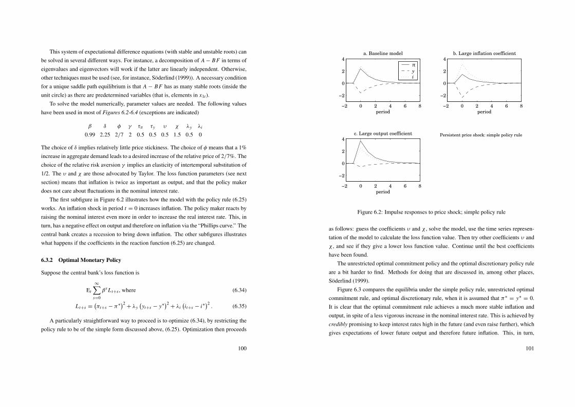
This system of expectational difference equations (with stable and unstable roots) canbe solved in several different ways. For instance, a decomposition of A − B F in terms ofeigenvalues and eigenvectors will work if the latter are linearly independent. Otherwise,other techniques must be used (see, for instance, Soderlind (1999)). A necessary conditionfor a unique saddle path equilibrium is that A − B F has as many stable roots (inside theunit circle) as there are predetermined variables (that is, elements in x1t ).

To solve the model numerically, parameter values are needed. The following valueshave been used in most of Figures 6.2-6.4 (exceptions are indicated)

β δ φ γ τπ τy υ χ λy λi

0.99 2.25 2/7 2 0.5 0.5 0.5 1.5 0.5 0

The choice of δ implies relatively little price stickiness. The choice of φ means that a 1%increase in aggregate demand leads to a desired increase of the relative price of 2/7%. Thechoice of the relative risk aversion γ implies an elasticity of intertemporal substitution of1/2. The υ and χ are those advocated by Taylor. The loss function parameters (see nextsection) means that inflation is twice as important as output, and that the policy makerdoes not care about fluctuations in the nominal interest rate.

The first subfigure in Figure 6.2 illustrates how the model with the policy rule (6.25)works. An inflation shock in period t = 0 increases inflation. The policy maker reacts byraising the nominal interest even more in order to increase the real interest rate. This, inturn, has a negative effect on output and therefore on inflation via the “Phillips curve.” Thecentral bank creates a recession to bring down inflation. The other subfigures illustrateswhat happens if the coefficients in the reaction function (6.25) are changed.

6.3.2 Optimal Monetary Policy

Suppose the central bank’s loss function is

Et

∞∑s=0

βs L t+s , where (6.34)

L t+s =(πt+s − π∗

)2+ λy

(yt+s − y∗

)2+ λi

(it+s − i∗

)2. (6.35)

A particularly straightforward way to proceed is to optimize (6.34), by restricting thepolicy rule to be of the simple form discussed above, (6.25). Optimization then proceeds

100

−2 0 2 4 6 8

−2

0

2

4a. Baseline model

period

πy

i

−2 0 2 4 6 8

−2

0

2

4b. Large inflation coefficient

period

−2 0 2 4 6 8

−2

0

2

4c. Large output coefficient

period

Persistent price shock: simple policy rule

Figure 6.2: Impulse responses to price shock; simple policy rule

as follows: guess the coefficients υ and χ , solve the model, use the time series represen-tation of the model to calculate the loss function value. Then try other coefficients υ andχ , and see if they give a lower loss function value. Continue until the best coefficientshave been found.

The unrestricted optimal commitment policy and the optimal discretionary policy ruleare a bit harder to find. Methods for doing that are discussed in, among other places,Soderlind (1999).

Figure 6.3 compares the equilibria under the simple policy rule, unrestricted optimalcommitment rule, and optimal discretionary rule, when it is assumed that π∗

= y∗= 0.

It is clear that the optimal commitment rule achieves a much more stable inflation andoutput, in spite of a less vigorous increase in the nominal interest rate. This is achieved bycredibly promising to keep interest rates high in the future (and even raise further), whichgives expectations of lower future output and therefore future inflation. This, in turn,

101

−2 0 2 4 6 8

−2

0

2

4a. Simple policy rule

period

πy

i

−2 0 2 4 6 8

−2

0

2

4b. Commitment policy

period

−2 0 2 4 6 8

−2

0

2

4c. Discretionary policy

period

Persistent price shocks

Figure 6.3: Impulse responses to price shock: simple rule, optimal commitment policy,and discretionary policy

gives lower inflation and output today. The discretionary equilibrium is fairly similar tothe simple rule in this model. Note that there is no constant “inflation bias” when targetlevels are at their natural levels (zero) as they are in these figures. The discretionary rule isstill different from the commitment rule (they are, after all, outcomes of different games).The intuition is that there is a time-varying “bias” since the conditional expectations ofoutput and inflation in the next periods (their “conditional natural rates”) typically differfrom the target rates (here zero).

Figure 6.4 makes the same type of comparison, but for a positive demand shock, −εyt .In this case, both optimal rules “kill” the demand shock, which is seen almost directlyfrom (6.24): any shock εyt could be met by increasing it by γ εyt . In this way output isunaffected by the shock, and there will then be no effect on inflation either, since the onlyway the demand shock can affect inflation is via output (see (6.23)). This is very similar

102

−2 0 2 4 6 8

−2

0

2

4a. Simple policy rule

period

πy

i

−2 0 2 4 6 8

−2

0

2

4b. Commitment policy

period

−2 0 2 4 6 8

−2

0

2

4c. Discretionary policy

period

Persistent demand shocks

Figure 6.4: Impulse responses to positive demand shock: simple rule, optimal commit-ment policy, and discretionary policy

to the static model discussed above: the demand shock drives both prices and output inthe same direction and should, if possible, neutralized. Of course, the result hinges onthe assumption that the policy maker is not averse to movements in the nominal interestrate, that is, λi = 0 in (6.35). (It can be shown that this case can be approximated in thesimple policy rule (6.25) by setting the coefficients very high.) Many studies indicate thatcentral banks are unwilling to let the nominal interest rate vary much. This is sometimesinterpreted as a concern for the banking sector, and sometimes as due to uncertainty aboutthe state of the economy and/or the effect of policy changes on output/inflation. In anycase, λi > 0 is often necessary in order to make this type of model fit the observedvariability in nominal interest rates.

103

A Derivations of the Aggregate Demand Equation

The period utility function is

U (Ct) =At

1 − γC1−γ

t , (A.1)

where At is a taste shift parameter. The Euler equation for optimal consumption is

∂U (Ct)

∂Ct= βEt

[∂U (Ct+1)

∂Ct+1Qt+1

], (A.2)

where Qt+1 is the gross real return.The marginal utility of Ct is

∂U (Ct)

∂Ct= AtC

−γt , (A.3)

so the optimality condition can be written

1 = βEt Qt+1At+1

At

(Ct+1

Ct

)−γ

= βEt exp (ln Qt+1 +1 ln At+1 − γ ln Ct+1 + γ ln Ct) . (A.4)

Assume that ln Qt+1, ln At+1, and ln Ct+1 are jointly normally distributed. (Recall Eexp (x) =

exp (Ex + Var (x) /2) is x is normally distributed.) Take logs of (A.4) and rewrite it as

0 = lnβ + Et ln Qt+1 + Et1 ln At+1 − γEt ln Ct+1 + γ ln Ct

+ Vart (ln Qt+1 + ln At+1 − γ ln Ct+1) /2, or (A.5)

Et ln Ct+1 = ln Ct +1γ

Et ln Qt+1 +1γ

Et zt+1,

where Et zt+1 = lnβ+Et1 ln At+1+Vart(.). The most important part of Et zt+1 is Et1 ln At+1.If ln At+1 = ρ ln At + ut+1, then Et1 ln At+1 = (ρ − 1) ln At , so the AR(1) formulationcarries over to the expected change, but the sign is reversed if ρ > 0.

Bibliography


104

King, R. G., 1993, “Will the New Keynesian Macroeconomics Resurrect the IS-LMModel?,” Journal of Economic Perspectives, 7, 67–82.





Soderlind, P., 1999, “Solution and Estimation of RE Macromodels with Optimal Policy,”European Economic Review, 43, 813–823.


105

7 Empirical Measures of the Effect of Money on Output

Reference: Romer 5.6, Walsh (1998) 1, Mishkin (1997) 25, Isard (1995), Meese (1990),and Obstfeldt and Rogoff (1996) 9.1

7.1 Some Stylized Facts about Money, Prices, and Exchange Rates

1. The correlation between long run inflation and money growth is almost one acrosscountries (BW Fig 8.9a).

2. The correlation between short run inflation and money growth is more uncertain(BW Fig 10.10).

3. There is no clear long run correlation between inflation and the growth of real outputor between money growth and the growth of real output.

4. Money stock innovations and output innovations are correlated. Money stock changesseems to lead output changes. Most of this correlation is between output and “insidemoney” (created within the banking system, for instance, deposits).

5. PPP does not hold, except possibly for long horizons. Realignments seem to havelong lasting (although perhaps not permanent) effects on the real exchange rate.(BW Fig 8.9b)

6. Countries with weak current accounts, and rapidly expanding money supply oftenexperience depreciation of the exchange rate.

7. Real exchange rates are much more volatile under flexible exchange rate regimesthan under fixed exchange rates. Real and nominal exchange rates are very stronglycorrelated (this is evidence of monetary non-neutrality only if we can prove exis-tence of important nominal shocks). (Isard Fig 3.2 and 4.2)

8. The log exchange rate behaves almost like a random walk (that is, ln St ≈ ln St−1 +

ut ). Equations for predicting ln St − ln St−1 typically have R2 < 0.1.

106

9. The monetary contraction in many countries after the 1929 crash in the US canprobably be regarded as exogenous shifts. Countries which left the gold standardearly had weaker recessions. (OR Fig 9.10)

10. Most contracts are written in nominal terms, and prices are typically changed fairlyseldom—even at the fairly high inflation rates of the late 1970s. This seems tochange as we move into very high inflation rates. The way it changes is by indexa-tion or “dollarization.”

11. Sharp exogenous monetary contractions (or a sudden and unexpected increase inthe short interest rates by the central bank) seems to have an effect on output andemployment which may last for years. (Walsh Fig 1.3)

7.2 Early Studies of the Effect of Money on Output

Early Keynesians (until the 1960s, say) thought that money has little effect on output.There were several reasons for this. First, nominal interest rates (on high grade bonds)were very low during the Great Depression, but that did not appear to boost output. Sec-ond, investment and consumption regressions showed very little effect of nominal interestrates.

The idea that the Great Depression was a period loose monetary policy was heavilychallenged by Friedman and Schwartz (1963a). They showed that the decline in moneysupply was the largest ever in US history. (A possible counter argument to this is that themonetary base changed fairly little, and that most of the change in the money aggregateswere due to the fact that the public chose to hold more cash and less deposits, and thatbanks chose to hold more reserves.)

Another weak spot of the early Keynesian interpretation of the Great Depression isthat it is based on low nominal interest rates. Prices were falling, so the real interest rateswere actually very high, perhaps as high as 10%, which could be interpreted as a verytight monetary policy.

107

7.3 Early Monetarist Studies of the Effect of Money on Output

7.3.1 Friedman&Schwartz and St. Louis Equations

Friedman and Schwartz (1963a) and Friedman and Schwartz (1963b) study 100 yearsof US data and find that money aggregates lead output, in the sense that all recessionswere preceded by declining money growth rates. However, the response to money growthchanges showed “long and variable lags.” They also argue that many of the money sup-ply changes can be regarded as exogenous with respect to output (changes within themonetary sector).

The St. Louis equation (see, for instance, Andersen and Jordan (1968)) is a regres-sion of output (growth) on current and lagged money (growth) and perhaps some othervariables. This can be thought of as a formalization of the approach of Friedman andSchwartz, although no attention is paid to whether the money supply changes are exoge-nous or not. In its simplest form it is

yt =

∑s=0

αsmt−s + εt , (7.1)

and the αs coefficients are sometimes interpreted as the effect of the money stock, mt−s ,on output, yt . (Initially, St. Louis equations were used to explain nominal output, but herethe focus is on real output.)

The St. Louis equation is not a structural model; it is a reduced form. Monetaristswould perhaps argue that the transmission mechanism from money to output is very com-plex, and that it makes sense to use (7.1) since it can potentially summarize the effects.Keynesians would perhaps be more “structural” in the sense that their view of the trans-mission mechanism is quite clear: money supply affects the interest rate (the LM equa-tion), which in turn affects output (IS equation).

Any causal interpretation of the correlation between money and output, or of the St.Louis equation relies on the assumption that most movements in the money stock are dueexogenous forces and not due to changes in output. These exogenous forces could bepolicy shocks or shifts in money demand which are not caused by output.

108

7.3.2 On the Interpretation of Cov(yt ,mt ) I: Reverse Causality

The problem with a causal interpretation of the correlation between money and output,or of the St. Louis equation, is that most of the correlation between money and output is

between output and “inside money” (deposits which is money created within the privatebanking system, as opposed to the monetary base which is outside money).

It is possible that banks extend more loans (which generates deposits) as the businessconditions are about to pick up. The correlation between money and output is then due toreverse causality as discussed in King and Plosser (1984). The idea is that money may nothave any effect on output, but output affects money aggregates positively, which explainsthe positive correlation of output and money. For this to make sense, it must be the casethat the central bank cannot, or does not want to, control the broad monetary aggregates.

Example 33 (Regressing output on money, two-way causality.) Suppose the structural

model of output and money is

yt = βmt + u yt

mt = γ yt + umt ,

where the shocks are assumed to be uncorrelated. Output and money are here allowed to

depend on each other (in the same period). The reduced form is[yt

mt

]=

11 − βγ

[1 β

γ 1

][u yt

umt

].

Suppose we run a very simple St. Louis equation

yt = αmt + εt ,

109

The least squares (LS) estimate of α is (in probability limit, plim)

plim αL S =Cov (mt , yt)

Var (mt)

=Cov

(γ u yt + umt , u yt + βumt

)Var

(γ u yt + umt

)=γVar

(u yt)+ βVar (umt)

γ 2Var(u yt)+ Var (umt)

=γVar

(u yt)/Var (umt)+ β

γ 2Var(u yt)/Var (umt)+ 1

.

Example 34 (Exogenous money supply.) If mt is exogenous, γ = 0, then plim αL S = β

in Example 33 and the regression coefficient captures the effect of money shocks on output.

This is the interpretation in Friedman and Schwartz (1963a). We get the same result if

Var(u yt)/Var(umt) → 0, that is, when most of the movements in output (and money) is

caused by the exogenous money shocks, so money is once again essentially exogenous.

Example 35 (Output shocks dominate.) Conversely, Var(u yt)/Var(umt) → ∞ gives

plim αL S → 1/γ in Example 33 (use l’Hopital’s rule to show this), so the regression

coefficient merely reflects how money (and output) are both driven by output shocks (“re-

verse causality”).

The reverse causality story can be turned on its head, however. Suppose money dohave effect on output, but that the central bank tries to stabilize output, that is, output hasa negative effect on money supply. In this case, the correlation of money and output willunderestimate the effect of money on output.

Example 36 (Countercyclical policy.) From the reduced form in Example 33, we see that

output follows

yt =1

1 − βγu yt +

β

1 − βγumt .

Suppose β > 0, then a negative γ makes the effect of an output shock small. This gives

plim αL S < β, so the St. Louis equation has a negative bias in the direct effect of money

on output.

110

7.3.3 On the Interpretation of Cov(yt ,mt ) II: Common Driving Force

Instead of assuming that output affects money stock directly, it may be that there is a thirdvariable which drives both output and money. This will also make the interpretation ofmoney-output correlations very murky, since it gives an omitted-variables bias.

Example 37 (Regressing output on money, unobservable driving force.) Suppose the

structural model of output and money is

mt = zt + umt

yt = βmt + κzt + u yt

= (κ + β) zt + u yt + βumt

where the shocks are uncorrelated with each other and with zt . Money affects output if

β 6= 0, but output does not affect money. However, both money and output are driven by

the common factor zt . The LS estimate of α in the St. Louis equation, yt = αmt + εt , is

then

plim αL S =Cov (mt , yt)

Var (mt)

=Cov

(zt + umt , (κ + β) zt + u yt + βumt

)Var (zt + umt)

=(κ + β)Var (zt)+ βVar (umt)

Var (zt)+ Var (umt)

=(κ + β)Var (zt) /Var (umt)+ β

Var (zt) /Var (umt)+ 1.

This equals β only if zt is (effectively) a constant, Var(zt) /Var(umt) = 0, or if output is

not affected by zt , κ = 0, so there is no common driving force.

Example 38 (Unobservable driving force and “reverse causality.”) Suppose β = 0 in

Example 37, so money has no effect on output (nor has output any effect on money). In

this case, the estimate of α in the St. Louis equation, yt = αmt + εt , becomes

plim αL S =κVar (zt) /Var (umt)

Var (zt) /Var (umt)+ 1,

which has the same sign as κ . If we interpret yt as output in the next period, which

thus depends on today’s zt , then we have the case of King and Plosser (1984). Their

111

mechanism is that zt signals high future productivity, which leads to more purchases of

production factors today (needs to be accumulated in advance). This is a version of the

traditional “reverse causality,” with the twist that future output affects today’s money

demand.

Example 39 (Countercyclical policy.) Suppose Var(u yt) =Var(umt) = 0 in Example 37

and that the central bank sets κ = −β. This achieves complete stabilization of output,

and plim αL S = 0 in the St. Louis equation. In this case, the successful monetary policy

makes it look as if monetary policy cannot affect output.

One way of getting around the problem with the common driving force is to estimatean extended St. Louis equation, where output is related to both money and a vector ofother variables capturing the driving force, xt ,

yt =

∑s=0

αsmt−s +

∑s=0

βs xt−s + εt . (7.2)

Of course, this approach assumes that we can observe the relevant variables and that theyare exogenous. The problem with a direct reverse causality (direct effect of output onmoney, possibly with leads/lags) remains in this equation, however.

7.3.4 St. Louis Equation with Instrumental Variables

Suppose we could get exogenous indicators of the exogenous movements in monetarypolicy. As a first step, regress mt on the “instruments” and construct a series of fittedpolicy, mt . In a second step, use mt instead of mt in a regression like (7.1). This is theIV/2SLS method, which is consistent as long as the instruments are not driven by output.

The “trick” in the IV/2SLS method is to discard all variation in mt which is not drivenby the instruments. This side-steps all movements in mt which are due to reverse causality,that is, due to the output shock. The regression will then look at how output moves inresponse to the exogenous changes in money.

Example 40 (IV and the case of two-way causality.) Consider the model in Example 33,

and suppose we now that umt = At +εmt , where At are observable shifts in money supply.

112

Run a regression mt = λAt + ξt , where we get from the reduced form that

plim λ =Cov(At ,mt)

Var (At)

=

Cov(At ,γ

1−βγu yt +

11−βγ

At +1

1−βγεmt)

Var (At)

=1

1 − βγ,

since At is assumed to be uncorrelated with u yt and εmt . Form a fitted value of mt as

mt = λAt , or

mt =1

1 − βγAt ,

and use this instead of mt in the St. Louis regression, yt = αmt + εt . This gives a new

estimate

plim αiv =Cov

(mt , yt

)Var

(mt)

=

Cov(

11−βγ

At , u yt + βAt + βεmt

)Var

(1

1−βγAt

)= β,

where we once again use the fact that At is uncorrelated with u yt and εmt . This is the

correct value.

Romer and Romer (1990) went through the Fed’s minutes to identify (exogenous)policy shifts. They found six such policy shifts during the post war period. In each case,short interest rates increased, while money aggregates and output decreased. They thenestimated a St. Louis equation with both least squares and instrumental variables, wheredummies for these episodes were used as instruments for money. They found that theinstrumental variables method gave larger effects of money on output, as expected if thecentral bank uses money in a systematic way to stabilize output.

The analysis of Romer and Romer (1990) is very much like a formalization of whatFriedman and Schwartz (1963b) did: pick out a number of monetary contractions whichlook exogenous and study what happens to output after that. Overall, the evidence fromthe historical episodes in these and other studies point in the direction that money probably

113

have an effect on output. This conclusion is strengthened if we look at the reaction ofoutput of large exchange rate realignments (another type of monetary policy).

Example 41 (Summary of Romer and Romer (1990) and Romer 232-236.) Main issue:

to find instruments for exogenous shifts in monetary policy. The problem with possibly

endogenous money is circumvented by focusing on episodes of exogenous (according to

Romer and Romer) shifts in monetary policy: September 1955, December 1968, April

1974, August 1978, and October 1979. According to the authors, these monetary con-

tractions were brought about by a desire to take down inflation, with little concern about

the effects on output. To investigate if there really were monetary contractions, univariate

forecasting equations for log money stock where estimated

1mt =

24∑s=1

αs1mt−s + ut

on monthly postwar data. Dynamic forecast for each period of 36 months after the 5 break

dates indicate that the money stock were a lot lower (in data) than predicted: there seem

to have been contractions. Also, the interest rates show fairly consistent increases over

the same 36 months, so any effect on output could be consistent with either a monetarist or

a Keynesian model. To see if theses contractions mattered for output, a St. Louis equation

was estimated

1yt = a + bt +

24∑s=1

ci1yt−s +

24∑s=0

di1mt−s,

with OLS and instrumental variables (IV). The instruments were a constant, a trend,

1yt−s , 1mt−s , and {P St−s}36s=0, where P St = 1 if t is one of the five policy shift dates,

and zero otherwise. If mt is affected (negatively - to stabilize output) by Yt , OLS on the

output equation gives a downward bias in di . The IV approach should give consistent es-

timates if the P St are not affected by output (the policy shifts were exogenous with respect

to output, driven by concern about inflation, and inflation does not affect output per se),

and if P St affects output via money only (probably reasonable). The result is that dI V is

larger than dO L S .

114

7.3.5 Dynamic Effects and Causality

Suppose the structural model consists of a reaction function where money is predeter-mined

mt =

p∑s=1

γs yt−s +

p∑s=1

δsmt−s + umt (7.3)

and a somewhat extended St. Louis equation

yt = α0mt +

p∑s=1

αsmt−s +

p∑s=1

βs yt−s + u yt . (7.4)

The shocks are assumed to be uncorrelated.This is a “fully recursive” system of simultaneous equations, so least squares on (7.3)

and (7.4) separately is consistent. The reason is that the simultaneity problem is assumedaway: money is not contemporaneously affected by the output shock. It is also assumedthat the lagged money and output capture all relevant common driving forces, so there isno omitted-variables bias.

However, if we care about more than just the impact effect of money supply shocks,then money is endogenous in the economic sense since we have the following chain ofeffects: umt → mt → yt → mt+1 → yt+1 →... We therefore need to estimate bothequations in order to trace out the effect of a monetary policy shock on output. This is theVAR approach discussed below.

7.4 Unanticipated or Anticipated Money∗

Reference: Romer 6.4, Mishkin (1983) 6, and Barro (1977).Both the new monetarist (Lucas’ model for the Phillips curve ) and new Keynesians

(“micro based” models of nominal rigidities) emphasize the distinction between antici-pated and unanticipated policy changes. The theoretical predictions, based on rationalexpectations, are that anticipated policy changes should have no or only small effects onoutput, while unanticipated changes could have large effects.

For simplicity, assume that the structural model for output is

yt =

p∑s=0

αs (mt−s − Et−s−1mt−s)+ u yt , (7.5)

115

so output depends on money stock surprises and an output shock, u yt .The money supply rule is assumed to depend on past information and a policy shock;

money supply is predetermined in relation to output

mt = γ ′zt−1 + umt ⇒ Et−1mt = γ ′zt−1. (7.6)

The output and policy shocks are uncorrelated. The vector zt−1 typically involves laggedoutput, money supply, and some other variables. As in (7.3) and (7.4), the econometricsimultaneity problem is assumed away by making money supply predetermined in relationto the output shock.

Use the policy rule (7.6) in the output equation (7.5)

yt =

k∑s=0

αs(mt−s − γ ′zt−s−1

)+

n∑s=0

θ ′zt−s−1 + u yt , (7.7)

where θ = 0 if only unanticipated money matters. Suppose the system (7.6) and (7.7)is estimated jointly and rational expectations is imposed (restricting γ to be the same inboth equations). It is then straightforward to test if θ = 0. Mishkin’s results indicate thatanticipated policy does matter.

Under the maintained hypothesis that only unanticipated money matters, only the αs

coefficients are needed in order to study the effect on money on output. This is differentfrom (7.3) and (7.4), where we needed the whole system. The reason is that in (7.5)-(7.6)the feedback from yt to mt+1 (due to an initial money supply shock umt ) has no effect onyt+1.

7.5 VAR Studies

7.5.1 VAR Models and Simultaneous Equations Systems∗

The VAR approach is an attempt to capture the main time series properties of moneyand output (and sometimes other variables) at the same time as enough restrictions areimposed to identify exogenous policy shifts. It is basically an attempt to estimate a systemof simultaneous structural equations.

For instance, (7.3) and (7.4) is a typical VAR model. In order to illustrate how VARmodels are handled, we look at that simple bivariate system of output and money once

116

again. The two (structural, it is assumed) equations can be written

B0

[mt

yt

]= B1

[mt−1

yt−1

]+ ...+ Bp

[mt−p

yt−p

]+

[umt

u yt

], (7.8)

B0, ..., Bp are 2 × 2 matrices.The parameters (B0, ..., Bp, and the covariance matrix of the shocks) cannot be esti-

mated without imposing some identifying restrictions. In fact, all data can tell us is theparameters of the reduced form[

mt

yt

]= A1

[mt−1

yt−1

]+ ...+ Ap

[mt−p

yt−p

]+ εt , (7.9)

The problem is that there may be many structural forms that generate the same reducedform.

By (7.8), the reduced form can be written as[mt

yt

]= B−1

0 B1

[mt−1

yt−1

]+ ...+ B−1

0 Bp

[mt−p

yt−p

]+ B−1

0

[umt

u yt

], (7.10)

so

Ai = B−10 Bi for i = 1, ..., p and Cov (εt) = B−1

0 Cov

([umt

u yt

])(B−1

0

)′

. (7.11)

In the structural form (7.8), there are (1 + p) 4 coefficients in B0, ..., Bp and 3 parametersin covariance matrix of the structural shocks. In the reduced form (7.10), there are p4coefficients in A1, ..., Ap and 3 parameters in covariance matrix of the reduced formshocks. We therefore need to impose at least 4 restrictions to calculate the parametersin the structural form.

The following is a common set of restrictions. First, the structural shocks are un-correlated (one restriction, the off-diagonal element in the covariance matrix is zero).This means that the structural shocks have an economic interpretation as money or outputshocks. Second, the diagonal elements of B0 are unity (two restrictions); alternatively wecould assume that the variances of the structural shocks are unity. Third, B0 is triangu-lar. Often (see, for instance, Sims (1980))), the assumption has been that money is not

117

contemporaneously affected by output, so B0 has the form

B0 =

[1 0−α0 1

]. (7.12)

Using (7.12) in (7.8) gives us a system on the same form as (7.3) and (7.4). Asdiscussed before, these equations can be estimated with LS as they stand. Alternatively,the reduced form (7.9) can be estimated with LS. Imposing the assumptions allows us tosolve for the structural parameters (typically a matter of solving non-linear equations, butcan be simplified by using some straightforward matrix decompositions like the Choleskydecomposition).

This illustrates that the VAR does not allow us to escape the tricky question of endoge-nous money, or more generally, monetary policy. The simultaneous equations bias maytherefore affect the VAR estimate—if the identifying assumptions we make are wrong.Including lagged money and output in both equations is an attempt to control for commonmovements in money and movements which are driven common factors (to get away froma potential omitted-variables bias).

Once we have an estimate of the structural form (7.8), we may trace out the effect on,for instance, output of shocks to monetary policy (“impulse response function”). We mayalso calculate how large a fraction of the variance of the forecast error of output that isexplained by the monetary policy shocks (“variance decomposition”).

7.5.2 Typical Results from VAR Studies of Money and Output

The typical result for the US on quarterly data for the last 30 years or so is that output hasa humped-shaped response to umt which may last for several years. However, monetarypolicy shocks seems to have accounted for a fairly small fraction of the variance of output,in particular after 1982. This does not, of course, mean that systematic monetary policyhas not been important or that monetary policy shocks cannot be important. For the latter,the impulse response function is much more informative than the variance decomposition.It is unfortunate that the VAR analysis typically says very little about the importance ofthe systematic (feedback) part of policy, which by many is believed to be very important(partly in opposition to the idea that only unanticipated money matters).

Some authors (for instance, Bernanke and Blinder (1992)) argue that M1 is not a goodproxy for the monetary policy instrument, and that a short nominal interest rate should

118

be used instead. First, there is evidence (see, for instance, Sims (1980)) that if output,money, and the nominal interest rate are included in a VAR, then money can no longer helppredict output, but that interest rates help predict both output and money. (This suggeststhat much of the movements in monetary aggregates are endogenous, not exogenous asoften assumed in macro models of monetary policy.) Second, the impulse responses tomoney aggregates like US M1 is often weird: a positive innovation in M1 gives a declinein output and an increase in nominal interest rates (see, for instance, Eichenbaum (1992)).In contrast, a positive shock to the federal funds rate gives decline in output, which seemsmuch more reasonable. Third, many analysts argue that most central banks discuss andset monetary policy in terms of a short interest rate.

Often, the dynamic response to a policy shock (stricter policy) is that the price levelincreases instead of decreases: the price puzzle. This is often the case when a short interestrate is taken to be the policy instrument. The reason is probably that the VAR contains toolittle information compared to what the policy makers use. Including a commodity price“solves” the puzzle. The interpretation is that the central bank reacts to commodity priceincreases (by raising the interest rate/decreasing money supply) since they signal futureinflation. Suppose the monetary policy is unable to “kill” the inflation impulse completely.Unless you control for the commodity prices, it will appear as if tighter monetary policyleads to higher inflation. (See Walsh Fig 1.4)

Critique against VAR models: too little forward looking information included (assetprices?), policy shocks differ wildly between different studies, relatively little informationabout the effect of systematic policy, what if policy changes? (Lucas critique).

7.6 Structural Models of Monetary Policy

Reference: Fuhrer and Moore (1995), Fuhrer (1997), Soderlind (2000), and Clarida, Galı,and Gertler (1998).

Another line of research is to estimate a structural economic model directly (althoughthe requirement for the label “structural” may have shifted over time). Of course, thereis a long tradition of estimating AS-AD (IS-LM) models with adaptive expectations. Re-cently, this have gained new popularity, but we have also seen a number of papers estimat-ing similar models while allowing for rational expectations. Many central banks still usefairly large macro models, even if there is a tendency towards smaller models (in order to

119

handle rational expectations, among other things).Consider the simple model

πt = βEtπt+1 + δφyt + δεπ t (7.13)

Et yt+1 = yt +1γ(it − Etπt+1)+ εyt (7.14)

it = χπt + υyt + εi t . (7.15)

The first equation comes from a Calvo model of price setting for a firm under monopolisticcompetition; the second from the intertemporal optimality condition for a consumers (plusthe assumption that consumption equals output); and the third is Taylor’s policy rule,which describes how the central banks sets the short nominal interest rate.

It is clear that this is a complicated model to estimate: there is plenty of simultaneity,and expectations about future values are needed.

This model can be estimated by maximum likelihood by specifying the distributionof the shocks (επ t , εyt , and εi t ). The MLE is found by iteration on the following steps(i) guess a vector of parameters (β, δφ, γ , χ , υ, and the variances of the three shocks);(ii) solve for the equilibrium and times series process (of πt , yt , and it ); (iii) evaluate thelikelihood function; (iv) improve the guess of the parameter vector. This gives a set ofestimates where rational (model consistent) expectations have been imposed. A possiblealternative is to use survey information as proxies for some or all expectations.

Another approach is taken by Clarida, Galı, and Gertler (1998) who want to estimatethe monetary policy rule (“reaction function”) for several countries. They specify a policyrule for the short interest rate, it , of the form

it = β Et πt+12 + γ Et yt + ρit−1 + ut , (7.16)

where Et yt is the best estimate of the current output gap and where πt+12 is the inflationover the next twelve months. This formulation is can be seen as an approximation of theoptimal policy in many models where there is some price stickiness and where the centralbank wants to stabilize inflation and output, but also avoiding excessive movements in theshort interest rate. The equation is estimated with an instrumental variables method. Tosee why that makes sense, not that we can rewrite (7.16) as

it = βπt+12 + γ yt + ρit−1 + ut + εt+n, (7.17)

120

where εt+n is a linear combination of the surprise in inflation, πt+12 −Et πt+12, and in theoutput gap, yt−Et yt . The new residual in (7.17), ut+εt+n , is clearly not uncorrelated withthe regressors, so we need to apply an instrumental variables method. All information att or earlier should be valid instruments.

Clearly, this approach allows us to understand the monetary policy rule only. To seehow a policy change, for instance, a shock ut to (7.16) affects output and inflation, wehave to estimate the rest of the model.

Bibliography

Andersen, L. C., and J. L. Jordan, 1968, “Monetary and Fiscal Actions: A Test of TheirRelative Importance in Economic Stabilization,” Federal Reserve Bank of St. Louis

Review, 50, 11–24.

Barro, R. J., 1977, “Unanticipated Money Growth and Unemployment in the UnitedStates,” American Economic Review, 67, 101–115.

Bernanke, B. S., and A. S. Blinder, 1992, “The Federal Funds Rate and the Channels ofMonetary Transmission,” American Economic Review, 82, 901–921.

Clarida, R., J. Galı, and M. Gertler, 1998, “Monetary Policy Rules in Practice: SomeInternational Evidence,” European Economic Review, 42, 1033–1067.

Eichenbaum, M., 1992, “Comment on ’Interpreting the Macroeconomic Time SeriesFacts: The Effects of Monetary Policy’ by Christopher Sims,” European Economic

Review, 36, 1001–1011.

Friedman, M., and A. J. Schwartz, 1963a, A Monetary History of the United States, 1867-

1960, Princeton University Press, Princeton.

Friedman, M., and A. J. Schwartz, 1963b, “Money and Business Cycles,” Review of Eco-

nomics and Statistics, 45, 32–64.

Fuhrer, J., and G. Moore, 1995, “Inflation Persistence,” Quarterly Journal of Economics,110, 127–159.

121

Fuhrer, J. C., 1997, “Inflation/Output Variance Trade-Offs and Optimal Monetary Policy,”Journal of Money, Credit, and Banking, 29, 214–234.


King, R. G., and C. Plosser, 1984, “Money, Credit and Prices in a Real Business CycleModel,” American Economic Review, 74, 363–380.

Meese, R. A., 1990, “Currency Fluctuations in the Post-Bretton Woods Era,” Journal of

Economic Perspectives, 4, 117–133.

Mishkin, F. S., 1983, A Rational Expectations Approach to Macroeconometrics, NBER.



Romer, C. D., and D. H. Romer, 1990, “New Evidence on the Monetary TransmissionMechanism,” Brookings Papers on Economic Activity, 1, 149–213.

Sims, C. A., 1980, “Macroeconomics and Reality,” Econometrica, 48, 1–48.

Soderlind, P., 2000, “Monetary Policy and the Fisher Effect,” Journal of Policy Mod-

eling, Forthcoming, also available as Working Paper No. 159, Stockholm School ofEconomics.


122

0 Reading List

Main references: Romer (1996) (Romer), Blanchard and Fischer (1989) (BF), and Ob-stfeldt and Rogoff (1996) (OR). For an introduction to many of the issues, see Burdaand Wyplosz (1997) (BW). Walsh (1998) (Walsh) is a more advanced text, and is recom-mended for further study.

Papers marked with (∗) are required reading.

0.1 Money Supply and Demand

1. ∗Lecture notes

2. ∗OR 8.1, 8.3.1-4 (MIU), and 9.1 (stylized facts) or ∗Walsh 2.3.1 (MIU)

3. ∗Romer 9.8 (cost of inflation)

4. Lucas (2000) (cost of inflation)

5. BF 4.2 and 4.5 (MIU)

Keywords: money multiplier, central bank intervention, traditional money demandequations, money in the utility function, Friedman’s rule.

0.2 Price Level and Nominal Assets

1. ∗Lecture notes

2. ∗OR 8.2 (seignorage) or ∗Walsh 4.3 (seignorage)

3. ∗OR 8.4.1 and 8.4.3-4 (exchange rates)

4. ∗Meese (1990) (exchange rate regressions)

5. BF 4.7 and 5.1 (seignorage)

123

6. Romer 9.7 (seignorage)

7. Isard (1995) 4 (PPP), 5 (UIP), and 8 (exchange rate regressions)

Keywords: price level in general equilibrium, superneutrality of money, Cagan’smodel with rational expectations, seignorage, exchange rate determination from moneydemand and UIP

0.3 Money and Prices in RBC Models

1. ∗Lecture notes

2. ∗Benassy (1995) (Long-Plosser model with money and predetermined wages)

3. Cooley and Hansen (1995) (RBC model with money and predetermined wages)

4. King and Plosser (1984) (reverse causality)

5. Walsh 3.3 (CIA) and 5.3.1 (wage rigidity in MIU models)

Keywords: RBC model with money and sticky prices, reverse causality, CIA.

0.4 Money and Monopolistic Competition

1. ∗Lecture notes

2. ∗OR 10.1 (GE with monopolistic competition)

3. ∗Romer (1993) (overview of New Keynesian models)

4. ∗King (1993) (overview of New Keynesian models)

5. BF 8.1 (GE with monopolistic competition)

6. Romer 6.6 and 6.10-15 (monopolistic competition, real rigidities)

7. BF 9.5 (real rigidities)

8. Walsh 5.3.2 (imperfect competition and price stickiness)

124

Keywords: general equilibrium in static model of monpolistic competition (Blanchard-Kiyotaki), menu costs, Nash equilibria with/without sticky prices, importance of ”realrigidities.”

0.5 Sticky Prices

1. ∗Lecture notes

2. ∗Rotemberg (1987) (adjustment costs for prices) or ∗Walsh 5.5 (inflation persis-tence)

3. ∗Roberts (1995)

4. Romer 6.5-9 (staggered prices, Caplin-Spulber)

5. BF 8.2-4 (staggered prices, Ss, Caplin-Spulber)

Keywords: quadratic adjustment costs for prices (Rotemberg), Calvo’s model of pricechanges, combining with “flex price” from monopolistic competition. (Advanced: Ssrules)

0.6 Monetary Policy

1. ∗Lecture notes

2. ∗OR 9.4-5 (Barro-Gordon model) or ∗Walsh 8.1-2 (Barro-Gordon)

3. ∗Taylor (1995) (Empirical analysis of transmission mechanism)

4. ∗Fischer (1996) (Costs of inflation)

5. ∗Obstfeld and Rogoff (1995) (Mirage of fixed exchange rates)

6. Bernanke and Mishkin (1997) (inflation targeting)

7. Fuhrer (1997) (inflation/output trade-off)

8. Romer 5.1-5 (IS-LM) and 9.6 (What can policy accomplish?)

125

9. BF 11.2 (traditional monetary policy issues) and 11.4 (Barro-Gordon model)

10. Walsh 5.4 (macro model for policy analysis), 8.4-5 (institutions), and 10.5 (macromodel for policy analysis again)

11. OR 9.2-3 (Dornbusch model)

Keywords: Mundell-Flemming model and choice of exchange rate regime, Barro-Gordon model of monetary policy (discretion and commitment), recent models for mon-etary policy,

Dornbusch model.

0.7 Empirical Measures of the Effect of Money on Output

1. ∗Lecture notes

2. ∗Walsh 1 (overview)

3. Romer 5.6 (selective overview)

Keywords: interpreting money-output correlations, anticipated or unanticipated money,VAR studies, “case studies” (Romer-Romer).

0.8 The Transmission Mechanism from Monetary Policy to Output

1. Mishkin (1995)

2. Walsh (1998) 7

3. Bernanke and Gertler (1995)

4. Bernanke (1983)

5. Romer and Romer (1990)

6. Stiglitz and Weiss (1981)

Keywords: money view, lending view, credit rationing (Stiglitz-Weiss).

126

Bibliography


Bernanke, B., 1983, “Nonmonetary Effects of the Financial Crisis in the Propagation ofthe Great Depression,” American Economic Reveiw, 73, 257–276.

Bernanke, B. S., and M. Gertler, 1995, “Inside the Black Box: The Credit Channel ofMonetary Policy Transmission,” Journal of Economic Perspectives, 9, 27–48.

Bernanke, B. S., and F. S. Mishkin, 1997, “Inflation Targeting: A New Framework forMonetary Policy,” Journal of Economic Perspectives, 11, 97–116.



Cooley, T. F., and G. D. Hansen, 1995, “Money and the Business Cycle,” in Thomas F.Cooley (ed.), Frontiers of Business Cycle Research, Princeton University Press, Prince-ton, New Jersey.

Fischer, S., 1996, “Why Are Central Banks Pursuing Long-Run Price Stability,” inAchieving Price Stability, pp. 7–34. Federal Reserve Bank of Kansas City.

Fuhrer, J. C., 1997, “Inflation/Output Variance Trade-Offs and Optimal Monetary Policy,”Journal of Money, Credit, and Banking, 29, 214–234.


King, R. G., 1993, “Will the New Keynesian Macroeconomics Resurrect the IS-LMModel?,” Journal of Economic Perspectives, 7, 67–82.

King, R. G., and C. Plosser, 1984, “Money, Credit and Prices in a Real Business CycleModel,” American Economic Review, 74, 363–380.

Lucas, R. E., 2000, “Inflation and Welfare,” Econometrica, 68, 247–274.

127

Meese, R. A., 1990, “Currency Fluctuations in the Post-Bretton Woods Era,” Journal of


Mishkin, F. S., 1995, “Symposium on the Monetary Transmission Mechanism,” Journal

of Economic Perspectives, 9, 3–10.

Obstfeld, M., and K. Rogoff, 1995, “The Mirage of Fixed Exchange Rates,” Journal of



Roberts, J. M., 1995, “New Keynasian Economics and the Phillips Curve,” Journal of

Money, Credit, and Banking, 27, 975–984.

Romer, C. D., and D. H. Romer, 1990, “New Evidence on the Monetary TransmissionMechanism,” Brookings Papers on Economic Activity, 1, 149–213.

Romer, D., 1993, “The New Keynesian Synthesis,” Journal of Economic Perspectives, 7,5–22.



Stiglitz, J. E., and A. Weiss, 1981, “Credit Rationing in Markets with Imperfect Informa-tion,” American Economic Review, 71, 393–410.

Taylor, J. B., 1995, “The Monetary Transmission Mechamism: An Empirical Frame-work,” Journal of Economic Perspectives, 9, 11–26.


128

Documents

MacAll