Embed Size (px)
Citation preview

MA50174 ADVANCED NUMERICALMETHODS
2007
M. A. Freitag(heavily based on lecture notes by C. J. Budd)

Contents
6 Initial Value Problems (IVPs) 53
6.1 Introduction . . . . . . . . . . . . . . . . . . . . . . . . . . . . . . 536.2 Quadrature . . . . . . . . . . . . . . . . . . . . . . . . . . . . . . 55
6.3 Non-stiff ordinary differential equations (ODEs) . . . . . . . . . . 566.3.1 The Forward Euler Method . . . . . . . . . . . . . . . . . 566.3.2 The Runge-Kutta method . . . . . . . . . . . . . . . . . . 62
6.3.3 The Stormer - Verlet method and geometric integration . . 696.4 Stiff Differential Equations . . . . . . . . . . . . . . . . . . . . . . 73
6.4.1 Definition . . . . . . . . . . . . . . . . . . . . . . . . . . . 736.4.2 Numerical Methods . . . . . . . . . . . . . . . . . . . . . . 74
6.4.3 The Backward-Euler Method... an A-stable stiff solver . . 776.4.4 The Trapezium Rule: a symmetric stiff solver . . . . . . . 78
6.4.5 The Implicit Mid-point Rule...an ideal stiff solver? . . . . . 806.4.6 Multi-step methods . . . . . . . . . . . . . . . . . . . . . . 81
6.5 Differential Algebraic Equations (DAEs) . . . . . . . . . . . . . . 83
7 Two Point Boundary Value Problems (BVPs) 857.1 Introduction . . . . . . . . . . . . . . . . . . . . . . . . . . . . . . 85
7.2 Shooting Methods . . . . . . . . . . . . . . . . . . . . . . . . . . . 867.3 Finite Difference Methods . . . . . . . . . . . . . . . . . . . . . . 91
7.3.1 Discretising the second derivative. . . . . . . . . . . . . . . 917.3.2 Different boundary conditions . . . . . . . . . . . . . . . . 92
7.3.3 Adding in convective terms . . . . . . . . . . . . . . . . . 967.4 Nonlinear Problems. . . . . . . . . . . . . . . . . . . . . . . . . . 977.5 Other methods . . . . . . . . . . . . . . . . . . . . . . . . . . . . 99
52
Chapter 6
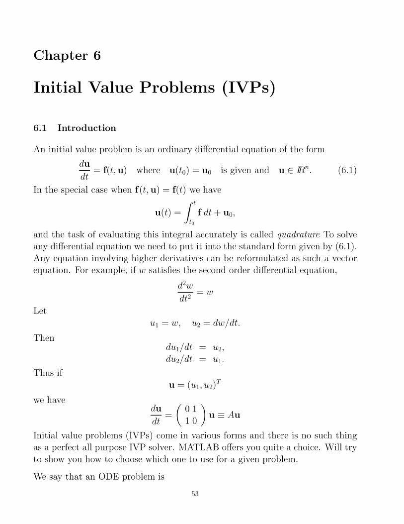
Initial Value Problems (IVPs)
6.1 Introduction
An initial value problem is an ordinary differential equation of the form
du
dt= f(t,u) where u(t0) = u0 is given and u ∈ IRn. (6.1)
In the special case when f(t,u) = f(t) we have
u(t) =
∫ t
t0
f dt + u0,
and the task of evaluating this integral accurately is called quadrature To solveany differential equation we need to put it into the standard form given by (6.1).
Any equation involving higher derivatives can be reformulated as such a vectorequation. For example, if w satisfies the second order differential equation,
d2w
dt2= w
Let
u1 = w, u2 = dw/dt.
Thendu1/dt = u2,du2/dt = u1.
Thus ifu = (u1, u2)
T
we havedu
dt=
(
0 1
1 0
)
u ≡ Au
Initial value problems (IVPs) come in various forms and there is no such thingas a perfect all purpose IVP solver. MATLAB offers you quite a choice. Will try
to show you how to choose which one to use for a given problem.
We say that an ODE problem is
53

1. Linear if f(t,u) is linear in u
2. Autonomous if f(t,u) ≡ f(u)
3. Non-stiff if all components of the equation evolve on the same timescale.This occurs (roughly) if the Jacobian matrix ∂f/∂u has all its eigenvalues
of similar size.
4. Stiff if different components of the system evolve on different time scales.
These are very common in chemical reactions with reactions going on atdifferent rates and in ODEs resulting from spatial discretisations of PDEs.
They also occur in PDEs where different modes (Fourier modes) evolve atvery different rates. Stiff problems are much harder to solve numerically
than non-stiff ones.
5. Hamiltonian if f takes the form
f = J−1∇H
where H(u) is the Hamiltonian of the system and
J =
[
0 −I
I 0
]
where I is the n2 × n
2 identity matrix.
Hamiltonian equations arise very commonly in rigid body mechanics, celes-
tial mechanics (astronomy) and molecular dynamics. To solve a Hamiltonianequation accurately over long time periods we must use special numerical
methods, such as symplectic or reversible methods.
All modern software for IVPs is a combination of three components
• The actual solver.
• A way of estimating the error of the solution.
• A step-size control mechanism.
Thus, the IVP solver attempts to use the best method to keep the (estimated)
error within a prescribed tolerance. Whilst it is essential to have some formof error control, no such method is infallible. The numerical solution of IVPs is
well covered in many texts, for example A.Iserles “A first course in the numericalsolution of differential equations.”
54
6.2 Quadrature
Suppose that f(t) is an arbitrary function, how accurately can we find
u =
∫ b
a
f(t)dt ? (6.2)
MATLAB determines this integral approximately by using a composite Simpson’srule.The idea behind this is as follows:
Suppose we take an interval of length 2h, without loss of generality this is theinterval [0, 2h].
• Evaluate f at the points 0, h, 2h
• Then approximate f by a parabola through these points, by using a quadraticinterpolant as in Chapter 3.
• Integrate this approximation to get an estimate for the integral of f .
This gives∫ 2h
0
fdx ≈h
6[f(0) + 4f(h) + f(2h)] ≡ Sh
This approximation is unreasonably accurate. It can be shown (see Froberg,
“Numerical Analysis”) that
|Sh −
∫ 2h
0
f(t)dt| =h5
90max |f (iv)(ξ)| where 0 < ξ < 2h (6.3)
The local error is proportional to h5 and to f (iv). The traditional use of Simpson’srule to evaluate (6.3) over [a, b] breaks this interval into sub-intervals of length
2h takes h constant between a and b and adds up the results to get a total errorestimated by
h4
90|b − a|max(|f (iv)|).
MATLAB is more intelligent than this and it uses an adaptive version of Simp-son’s rule. In this procedure h is chosen carefully over each interval to keep
the error estimated by (6.2) less than a user specified tolerance. In particularh is small when f is varying more rapidly and f (iv) is large. The integrals over
each sub-interval are then combined to give the total. This method is especiallyeffective if f has a singularity.The procedure uses the instruction
> i = quad (\mbox{@fun}, a,b,\mbox{tol})
55

where fun is the function to be integrated and tol is the tolerance. There isanother MATLAB code >quadl. This approximates f by a higher order polyno-mial. This is more accurate if f is smooth but unreliable if f has singularities.
6.3 Non-stiff ordinary differential equations (ODEs)
A non-stiff ordinary differential equation has components which all evolve on
similar time-scales. They are the easiest differential equations to solve by usinga numerical method. In particular they can often be solved by using explicit
methods that do not require the solution of nonlinear equations.
6.3.1 The Forward Euler Method
The oldest, easiest to apply and analyse, method for such problems is the explicitforward Euler method. Suppose that u satisfies the ODE
du
dt= f(t,u), u(0) = u0
• We take a small step h and approximate u((n − 1)h) by Un
• We set U1 = u0
• Now for each successive n we update Un through
Un+1 = Un + hf(t,Un) = Un + hf((n − 1)h,Un) (6.4)
This method is easy to use and each step is fast as no equations need to beevaluated and there is only one function evaluation per step. The Forward Eulermethod is still used when f is hard to evaluate and there are a large number of
simultaneous equations. Problems of this kind arise in weather forecasting. Themain problem with this method is that there are often severe restrictions on the
size of h.
Local Error.At each stage of the method a small error is made. These errors accumulate
over successive intervals to give an overall error. If the exact solution u(t) issubstituted into the equation (6.4), there is a mismatch E between the two
sides, called the local truncation error or LTE. This is a good estimate for theerror made by the method at each step. It is estimated by
|E| = |u(nh) − u((n − 1)h) − hf((n − 1)h,u((n− 1)h))| =h2
2|u′′(ξ)|, (6.5)
56

where(n − 1)h < ξ < nh
As in quadrature the local truncation error is proportional to a power of h, in
this case h2 and a higher derivative of u, in this case u′′. So, if u′′ is large (rapidchange), we must take h small to give a small error. The smaller the value of h is,
the more accurate the answer will be. (We will see later that h is also restrictedby stability considerations).
Global Error
Each time the method is applied an error is made and the errors accumulateover all the calculations. If we want to approximate u(T ) then need to make
T/h + 1 ≡ N calculations so that UN ≈ u(T ). We will call ε the global error if
ε = |UN − u(T )|, N =T
h+ 1.
This can be crudely estimated by
ε ≈Nh2
2max|u′′| ≈ Th max|u′′|.
We note that the overall error is proportional to h and to max|u′′|. We say that
this is an O(h) or a first order method.
The estimate we have obtained implies that the global error grows in proportion
to both h and T . In fact, this is rarely observed. In the worst case for someproblems the error grows in proportion to eT , when looking at periodic problemsit can grow like T 2 and for problems with a lot of symmetry, the errors can
accumulate much more slowly so that the overall error may not grow at all withT .
We start by looking at the worst case analysis.We say that f is globally Lipshitz if there is a constant L such that
|f(t, y) − f(t, z)| < L|y − z| (6.6)
It can then be shown (see A. Iserles “A first course in the numerical solutionof differential equations”) that if |u′′| ≤ M then the global error has an upper
bound given by
ε ≤hM
2L
(
eLT − 1)
(6.7)
If T is fixed and h → 0 then the upper bound given in (6.7) shows that ε isproportional to h in this limit. In practice the Forward Euler method is rarely
used in this way. We often take h fixed and let T → ∞. This is very dangerousas errors can accumulate rapidly making the method unusable. In this case we
57

need a more careful control on the global growth of errors. This is the philosophybehind geometric integration based methods.
Variable time-stepping
As in the quadrature process, Euler’s method can be used with a variable stepsize. This allows some control over the local error. To do this we take a sequence
of (small) time steps, so that the solution is approximated at times tk with sothat Uk ≈ u(tk)
hk ≡ tk+1 − tk.
If we have an estimate for u′′(ξ), ξ ∈ [tk, tk+1] then hk is chosen so that at eachstep
E =h2
k|u′′|
2< TOL
where TOL is specified by the user. Of course, without knowing u(t) we do notknow u′′ in general. We can either estimate an upper bound a -priori to thecalculation or we can try to deduce its value (a-posteriori) from the numerical
calculation. This latter procedure often uses an error estimate call the Milnedevice. (See Iserles.)
58
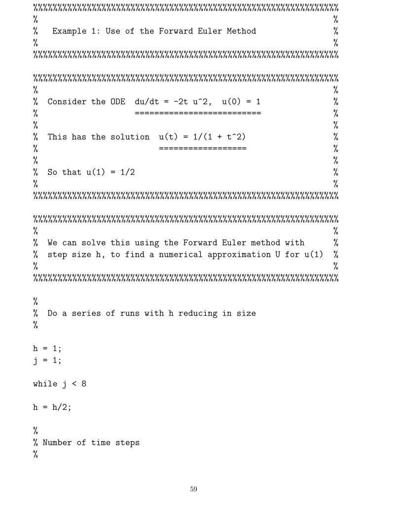
%%%%%%%%%%%%%%%%%%%%%%%%%%%%%%%%%%%%%%%%%%%%%%%%%%%%%%%%%%%%%%%
% %
% Example 1: Use of the Forward Euler Method %
% %
%%%%%%%%%%%%%%%%%%%%%%%%%%%%%%%%%%%%%%%%%%%%%%%%%%%%%%%%%%%%%%%
%%%%%%%%%%%%%%%%%%%%%%%%%%%%%%%%%%%%%%%%%%%%%%%%%%%%%%%%%%%%%%%
% %
% Consider the ODE du/dt = -2t u^2, u(0) = 1 %
% ========================== %
% %
% This has the solution u(t) = 1/(1 + t^2) %
% ================== %
% %
% So that u(1) = 1/2 %
% %
%%%%%%%%%%%%%%%%%%%%%%%%%%%%%%%%%%%%%%%%%%%%%%%%%%%%%%%%%%%%%%%
%%%%%%%%%%%%%%%%%%%%%%%%%%%%%%%%%%%%%%%%%%%%%%%%%%%%%%%%%%%%%%%
% %
% We can solve this using the Forward Euler method with %
% step size h, to find a numerical approximation U for u(1) %
% %
%%%%%%%%%%%%%%%%%%%%%%%%%%%%%%%%%%%%%%%%%%%%%%%%%%%%%%%%%%%%%%%
%
% Do a series of runs with h reducing in size
%
h = 1;
j = 1;
while j < 8
h = h/2;
%
% Number of time steps
%
59

N = 1/h + 1;
U = zeros(1,N);
t = zeros(1,N);
U(1) = 1;
t(1) = 0;
for i=2:N
%
% Euler step
%
t(i) = h + t(i-1);
U(i) = U(i-1) - 2*h*t(i-1)*U(i-1)^2;
end
hh(j) = h;
%
% Error
%
er(j) = U(N)-1/2;
j = j+1;
end
A = [hh’ er’]
plot(hh,er)
----------------------------------------------------------------------------
%
% The resulting solution has the following form
%
60
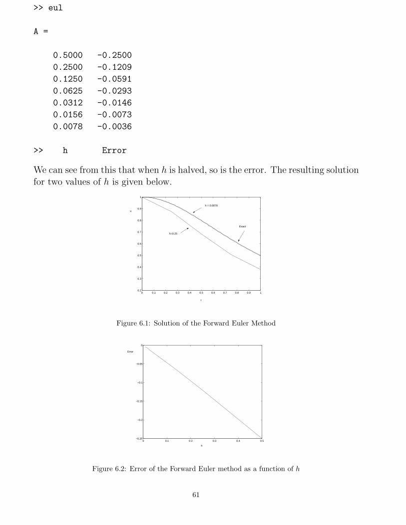
>> eul
A =
0.5000 -0.2500
0.2500 -0.1209
0.1250 -0.0591
0.0625 -0.0293
0.0312 -0.0146
0.0156 -0.0073
0.0078 -0.0036
>> h Error
We can see from this that when h is halved, so is the error. The resulting solutionfor two values of h is given below.
0 0.1 0.2 0.3 0.4 0.5 0.6 0.7 0.8 0.9 10.2
0.3
0.4
0.5
0.6
0.7
0.8
0.9
1
h=0.25
h = 0.0078
Exact
t
u
Figure 6.1: Solution of the Forward Euler Method
0 0.1 0.2 0.3 0.4 0.5−0.25
−0.2
−0.15
−0.1
−0.05
0
h
Error
Figure 6.2: Error of the Forward Euler method as a function of h
61

6.3.2 The Runge-Kutta method
A much more locally accurate method is the Runge-Kutta method. Its most
famous form is called the explicit fourth order Runge-Kutta or the RK4 method.
Suppose that the ODE isdu
dt= f(t,u). Then if we know Un, and set t = (n−1)h
the value of Un+1 is given by the sequence of operations
k1 = hf(t,Un)
k2 = hf
(
t +h
2, Un +
k1
2
)
k3 = hf
(
t +h
2, Un +
k2
2
)
k4 = hf(t + h, Un + k3)
Un+1 = Un +1
6(k1 + 2k2 + 2k3 + k4)
It can be shown that there is a value C which depends on f in a complex waysuch that a local truncation error E = |u(t + h) −Un+1| is bounded by
E ≤ Ch5
Over a large number of steps these errors accumulate as before to give a globalerror ε of the form:
ε ∼ C(eLT − 1)h4
The error is proportional to h4. Hence the name an order 4 method. The errorfor a given h is much smaller than for the Forward Euler method. This method
is VERY widely favoured as
1. It is easy to use and no equations need to be solved at each stage.
2. It is highly accurate for moderate h values
3. It is a one step method i.e. Un+1 only depends on Un
4. It is easy to start and easy to code.
For many people it is the ONLY method they ever use!! However, it has certaindisadvantages.
1. The function f must be evaluated four times at each iteration. This may be
difficult if f is hard or expensive to evaluate.
2. Errors accumulate rapidly as T increases.
3. The method cannot be used for stiff problems unless h is very small.
62

%%%%%%%%%%%%%%%%%%%%%%%%%%%%%%%%%%%%%%%%%%%%%%%%%%%%%%%%%%%%%%%
% %
% Example 2: Use of the 4th Order Runge-Kutta method %
% %
%%%%%%%%%%%%%%%%%%%%%%%%%%%%%%%%%%%%%%%%%%%%%%%%%%%%%%%%%%%%%%%
%%%%%%%%%%%%%%%%%%%%%%%%%%%%%%%%%%%%%%%%%%%%%%%%%%%%%%%%%%%%%%%
% %
% Consider the ODE du/dt = -2t u^2, u(0) = 1 %
% ========================== %
% %
% This has the solution u(t) = 1/(1 + t^2) %
% ================== %
% %
% So that u(1) = 1/2 %
% %
%%%%%%%%%%%%%%%%%%%%%%%%%%%%%%%%%%%%%%%%%%%%%%%%%%%%%%%%%%%%%%%
%%%%%%%%%%%%%%%%%%%%%%%%%%%%%%%%%%%%%%%%%%%%%%%%%%%%%%%%%%%%%%%
% %
% We can solve this using the RK4 method with %
% step size h, to find a numerical approximation for u(1) %
% %
%%%%%%%%%%%%%%%%%%%%%%%%%%%%%%%%%%%%%%%%%%%%%%%%%%%%%%%%%%%%%%%
%%%%%%%%%%%%%%%%%%%%%%%%%%%%%%%%%%%%%%%%%%%%%%%%%%%%%%%%%%%%%%%
% %
% The function is calculated in frk.m %
% %
%%%%%%%%%%%%%%%%%%%%%%%%%%%%%%%%%%%%%%%%%%%%%%%%%%%%%%%%%%%%%%%
%%%%%%%%%%%%%%%%%%%%%%%%%%%%%%%%%%%%%%%%%%%%%%%%%%%%%%%%%%%%%%%
% %
% Do a series of runs with h reducing in size %
% %
%%%%%%%%%%%%%%%%%%%%%%%%%%%%%%%%%%%%%%%%%%%%%%%%%%%%%%%%%%%%%%%
h = 1;
j = 1;
63

while j < 8
h = h/2;
%
% Number of time steps
%
N = 1/h + 1;
U = zeros(1,N);
t = zeros(1,N);
%
% Initial values
%
u(1) = 1;
t(1) = 0;
for i=2:N
%
% Runge-Kutta step
%
th = h/2 + t(i-1);
t(i) = h + t(i-1);
k1 = h*frk(t(i-1),U(i-1));
k2 = h*frk(th,U(i-1)+k1/2);
k3 = h*frk(th,U(i-1)+k2/2);
k4 = h*frk(t(i),U(i-1)+k3);
U(i) = U(i-1) + (k1+2*k2+2*k3+k4)/6;
end
64

hh(j) = h;
%
% Error
%
er(j) = U(N)-1/2;
j = j+1;
end
rat = er./hh.^4;
A = [hh’ er’ rat’]
plot(log(hh),log(abs(er)))
>> %%%%%%%%%%%%%%%%%%%%%%%%%%%%%%%%%%%%%%%%%%%%%%%%%%%%%%%%%%%%%%
>> %
>> % Test of the Runge-Kutta code
>> %
>> %%%%%%%%%%%%%%%%%%%%%%%%%%%%%%%%%%%%%%%%%%%%%%%%%%%%%%%%%%%%%%
>>
>> rung
A =
0.50000000000000 -0.00029847713504 -0.00477563416071
0.25000000000000 0.00001355253692 0.00346944945065
0.12500000000000 0.00000139255165 0.00570389155200
0.06250000000000 0.00000009811779 0.00643024720193
0.03125000000000 0.00000000640084 0.00671176833566
0.01562500000000 0.00000000040734 0.00683396495879
0.00781250000000 0.00000000002567 0.00689065456390
>> % h error error/h^4
>> %
>> % Note that error/h^4 is almost constant
>> %
>> diary off
65

0 0.1 0.2 0.3 0.4 0.5 0.6 0.7 0.8 0.9 10.5
0.6
0.7
0.8
0.9
1
t
u
I like to think of the RK4 method as being like a Ford Fiesta. It is easy to use,
everyone uses it and it is good value for money. If you are going to the shops (i.e.solving a relatively straightforward problem) it is the method to use. However,it won’t handle rough country nor would you want it for a very long drive.
To improve the accuracy the RK4 method is often used together with anotherhigher order method to estimate the local error and choose h accordingly. Sup-
pose that the value of Un+1 is given by an RK4 method. We could also use adifferent higher order method to calculate a separate value Un+1. Both Un+1
and Un+1 approximate u(t + h) so that:
Un+1 = u(t + h) + Ch5
Un+1 = u(t + h) + Dh6
Subtracting these estimates we have
‖ Un+1 − Un+1 ‖≤ |C|h5 + |D|h6
If h is small then |C|h5 ≈‖ Un+1 − Un+1 ‖ so the difference between the two
calculations gives an estimate for the local error of the RK4 method.We can now use this estimate as follows. Given Un and h
1. Using Un and step size h, calculate Un+1, Un+1 and En+1 =‖ Un+1−Un+1 ‖.
2. If TOL32 < En+1 < TOL then accept the step
3. If En+1 < TOL32 then set h = 2h and repeat from 1.
4. If En+1 > TOL then set h = h2 and repeat from 1.
This method keeps the local errors below the specified tolerance and also (due to
3) makes an efficient choice of step size. However it does not control the growthof errors. MATLAB uses such a Runge-Kutta 4,5 pair above the form devel-oped by Dormand & Prince in the ode45 routine. There is a similar (cheaper
66

but less accurate) Runge-Kutta 2,3 pair implemented in the routine ode23. Inthis routine you can set both the Absolute Tolerance (as above) or the RelativeTolerance TOL/ ‖ u ‖. You can the ode45 routine as follows:
>[t,U] = ode45 (@fun, trange, u_0, options)
Here t is the vector of times at which the approximate solution vector U is given.
Because the step-size h is chosen at each stage of the algorithm these times willnot (necessarily) be equally spaced. The function f(t, u) is specified by ‘fun’ andu0 is the vector of initial conditions. The time interval for the calculation is given
by trange. Setting
trange = [a b]
means that the ode45 routine will integrate the ODE between a and b, giving
its output at the (variable) time steps it computes. Alternatively
trange = [a: c: b]
leads to output at the points a, a+c, a+2c etc. The options command is optional,but it allows control over the operation of the ode45 routine. In particular you
can set the tolerances and/or request statistics on the solution. The options areset by using the odeset routine. For example if you want an absolute tolerance
of 10−12 you type
>options = odeset (‘AbsTol’, 1e^(-12}))
By default the absolute tolerance is 10−6 and the relative tolerance is 10−3.
67

%%%%%%%%%%%%%%%%%%%%%%%%%%%%%%%%%%%%%%%%%%%%%%%%%%%%%%%%%%%%%%%
% %
% Example 3: Use of ode45 %
% %
%%%%%%%%%%%%%%%%%%%%%%%%%%%%%%%%%%%%%%%%%%%%%%%%%%%%%%%%%%%%%%%
%%%%%%%%%%%%%%%%%%%%%%%%%%%%%%%%%%%%%%%%%%%%%%%%%%%%%%%%%%%%%%%
% %
% Consider the ODE du/dt = -2t u^2, u(0) = 1 %
% ========================== %
% %
% This has the solution u(t) = 1/(1 + t^2) %
% ================== %
% %
% So that u(1) = 1/2 %
% %
%%%%%%%%%%%%%%%%%%%%%%%%%%%%%%%%%%%%%%%%%%%%%%%%%%%%%%%%%%%%%%%
%%%%%%%%%%%%%%%%%%%%%%%%%%%%%%%%%%%%%%%%%%%%%%%%%%%%%%%%%%%%%%%
% %
% We can solve this using the ode45 method with %
% tolerances 1e-12,to find a numerical approximation for u(1)%
% %
%%%%%%%%%%%%%%%%%%%%%%%%%%%%%%%%%%%%%%%%%%%%%%%%%%%%%%%%%%%%%%%
options=odeset(’AbsTol’,1e-12,’RelTol’,1e-12);
trange = [0:0.05:1];
unit = [1];
[t,U] = ode45(@frk,trange,unit,options);
s = size(U);
err = U(s(1)) - 0.5
68

6.3.3 The Stormer - Verlet method and geometric integration
Geometric integration is a branch of numerical analysis which aims in part to
control global error growth of a numerical approximation over long times. Animportant application of geometric methods is to systems of the form
u = vv = −f(u)
}
{
u + f(u) = 0.
More generally, geometric methods can be applied to Hamiltonian systems forwhich
q = ∂H/∂p, p = −∂H/∂q
For the problem u + f(u) = 0 we set q = u, p = du/dt and
H = p2/2 + F (q) with F =
∫
fdq
Multiplying the differential equation by u and integrating with respect to timewe find that
H = u2/2 + F (u) = const.
More generally, in an autonomous Hamiltonian system, the Hamiltonian H is aconstant for all times. This is an example of a conservation law. Many physical
systems conserve particular quantities over all times. An excellent example ofthis is the solar system considered in isolation with the rest of the universe.
This obeys a complicated set of differential equations with complex (and indeedchaotic) solutions. However the total energy, angular momentum and linearmomentum are conserved for all time.
To retain the correct dynamics of such a system in a numerical approximationit is essential that the numerical approximation either exactly conserves the
same invariants or (more usually) the approximate equivalent of any conservedquantity varies from a constant by a small but bounded amount for all times.
If this occurs then the approximate solution is likely to be much closer to the
true solution for all times.
The Forward Euler method, RK4 and ode45 are not good at preserving suchconserved quantities. For example if we consider the system
u + f(u) = 0,u2
2+ F (u) = H
An application of the Forward Euler method with Un ≈ u((n − 1)h), V n ≈u((n − 1)h) gives
Un+1 = Un + hV n, V n+1 = V n − hf(Un)
69

so that
Hn+1 =(V n+1)2
2+ F (Un+1)
= [V n − hf(Un)]2 /2 + F (Un + hV n)
= Hn +h2
2
(
f(Un)2 + (V n)2∂f/∂u)
+ O(h3)
Thus H changes by
Hn+1 − Hn =h2
2
(
f(Un)2 + (V n)2∂f/∂u)
+ O(h3)
at each iteration. If ∂f/∂u > 0 then H is not conserved and increases at eachiteration as the errors accumulate so that the global error in H grows like nh2.
In the RK4 method we have the better result that
Hn+1 − Hn = h5Cn.
Again, in general the values of Cn are positive for many problems and the errors
in H accumulate over a large number of iterations, with global errors growinglike nh5. A widely used method which avoids many of these problems and has
excellent conservation problems is the Stormer - Verlet method (SV) . This is themethod of choice for simulations of celestial and molecular dynamics. Not onlyis it (much) better than RK4 for long-time integrations it is also much cheaper
and easier to code up as it only requires one function evaluation per time step. Itis also explicit, has global errors O(h2) and it is symmetric. The disadvantage of
the SV method is that it can only be used for a certain class of problems (thosewith a separable Hamiltonian) and it is not a black-box code i.e. it requires some
thought to use it. However this is precisely what mathematicians are paid to do!For the problem u + f(u) = 0 the SV method takes the following form
U ∗ = Un + h2V
n
V n+1 = V n − hf(U ∗)
Un+1 = U ∗ + h2V
n+1
In the SV method we have
Hn+1 − Hn = h3Dn.
This appears to be worse than RK4. However, unlike RK4 the errors DO NOT
accumulate and tend to cancel out. It can be shown that if H is the exactHamiltonian then
|Hn − H| < Dh3
where D does not depend on n. So, although H is not exactly conserved, the
method stays close to it for all time.We now apply this to an example with f(u) = u3.
70

%%%%%%%%%%%%%%%%%%%%%%%%%%%%%%%%%%%%%%%%%%%%%%%%%
% %
% Example 4: Stormer-Verlet method for %
% %
% u’’ + u^3 = 0, u(0) = 1, u’(0) = 0 %
% %
% In the exact eqn H is constant where %
% %
% H = (u’)^2/2 + u^4/4 %
% %
%%%%%%%%%%%%%%%%%%%%%%%%%%%%%%%%%%%%%%%%%%%%%%%%%
t(1) = 0;
U(1) = 1;
V(1) = 0;
h = 0.1;
H(1) = 1/4;
for i=2:100
Usta = U(i-1) + (h/2)*V(i-1);
V(i) = V(i-1) - h*Usta^3;
U(i) = Usta + (h/2)*V(i);
t(i) = t(i-1) + h;
H(i) = V(i)^2/2 + U(i)^4/4;
end
plot(t,H)
71

−1 −0.8 −0.6 −0.4 −0.2 0 0.2 0.4 0.6 0.8 1−1
−0.8
−0.6
−0.4
−0.2
0
0.2
0.4
0.6
0.8
1
u
v
Figure 6.3: A plot of U, V for the exact and numerical solution
0 1 2 3 4 5 6 7 8 9 100.25
0.252
t
H
Figure 6.4: A plot of H showing the bounded variation
72

6.4 Stiff Differential Equations
6.4.1 Definition
In a stiff differential equation the solution components evolve on very differenttimescales. This causes a problem as a numerical method, such as ode45, pos-
sibly chooses a step size for the most rapidly evolving component, even if itscontribution to the solution is negligable. This leads to very small step sizes,
highly inefficient computations and long waits for the user! The reason for thisis an instability in the method , where a small error may grow rapidly with eachstep.
Suppose we want to solve the ODE
u = f(u)
and the numerical method makes a small error e. We ask the question, howdoes e grow during the calculation? To answer this we start by looking at how
a small disturbance to the solution of the ODE changes. Suppose that e is sucha disturbance so that
d
dt(u + e) = f(u + e)
To leading order the perturbation e then satisfies the linear differential equation
du
dt+
de
dt= f(u) + Ae A =
∂f
∂u.
The perturbation growth is thus described by the differential equation
de
dt= Ae where A = ∂f/∂u. (6.8)
Now look at the ODE (6.8). This has the solution
e = eAte0
where e0 is the initial perturbation. So that if A = UΛU−1 then
e(t) = UeΛtU−1e0.
Alternatively, if A has eigenvalues λi and eigenvectors φi then
Aφi = λiφi φi : eigenvector
Thus if e0 is in the direction of φi so that
e0 = aφi
it follows thate(t) = aeλitφi
73

It follows further that‖ e(t) ‖= |a|eµit ‖ φi ‖
where µi is the real part of λi so that it is the real part of the eigenvalues which
control the growth of small perturbations.If |λi| is large and the real part of λi is less than zero, then the contribution
to e in the direction of the eigenvector φi rapidly decays to zero. After only ashort time the perturbation is dominated by the component in the direction ofthe eigenvector φj for which λj has the largest real part over all the eigenvalues.
We are now able to define what we mean by a stiff system.
DEFINITION
The system is stiff if the matrix A has eigenvalues λi for which
maxj
|λj| ≫ minj
|λj|.
Typically, in an application a ratio of the largest over the smallest absolutevalue of the eigenvalues of over 10 is considered to lead to a stiff system
In a physical system the components for which |λj| is large, and the real partof λj is negative, decay rapidly and are not seen in the solution apart from someinitial transients. It is therefore somewhat paradoxical that it is precisely these
components which lead to instabilities in the numerical scheme.This is anotherway of saying that the solution has components that evolve at very different
rates.
6.4.2 Numerical Methods
Now we look at a variety of numerical methods for solving the linear equation(6.8) so that we may compare the growth of perturbations to the numerical
solution with those of the true solution. First look at the performance of theForward Euler method when applied to this problem. We have
Un+1 = Un + hf(Un)
so that
Un+1 = Un + hAUn = (I + hA) Un
ThereforeUn = (I + hA)n−1 U1
But I + hA has the same eigenvectors φj as A and has eigenvalues
1 + hλj
74

So, the contribution to Un in the direction of the eigenvector φj grows as
(1 + hλj)n−1
or more precisely as |1 + hλj|n−1. In particular the errors caused by truncation
error or by rounding error only decay if |1 + hλj| < 1 for all λj .
We now find an extraordinary paradox. Suppose that λj is real and that
λj = −µ with µ ≫ 1
Then
eλjt = e−µt ≪ 1, if t ≫ 1
However
|1 + hλj|n = |1 − µh|n ≫ 1 if µh > 2 and n ≫ 1.
So the most rapidly decaying components of the perturbation to the continuoussolution are the components of Un which are growing most rapidly.
Stability of the Forward Euler method
We say the Forward Euler method with step size h is stable if given a matrix A
with eigenvalues λj with the real part less than zero then |1 + hλj| < 1 for allλj. In particular if λj are all real then the method is stable only if
h < 2/max|λj|
This is the restriction on h which means that solution errors do not grow. If his larger than this bound then errors grow and the method is unstable.
Here we see the problem. A component in the direction of φj with large |λj|and with real part λj < 0 dominates the choice of step size even though thiscomponent is very small.
• The LOCAL (TRUNCATION) ERROR that is made at each stage of thecalculation is given by
h2|u′′|
2.
So the error made at each stage depends on the SOLUTION. If all of theeigenvalues of A have negative real part then this error is ultimately dom-inated by the component of the solution that decays most slowly, which is
in turn determinated by the eigenvalue of A with the largest real part. Soithat it is the eigenvalue with the real part closest to zero, and typically this
is the eigenvalue with the smallest modulus.
75

• In contrast the GROWTH of the error as the iteration proceeds depends onthe eigenvalue of A with the largest modulus, even though this eigenvaluemay have a large negative real part and thus not contribute to the solution
in any way.
There are therefore two restrictions on h, it must be small both for accuracy ateach stage and for stability to stop the errors growing. Stiffness arises when the
restriction on h for stability is much more severe than the restriction for accuracy.
This introduces us to the ideas of stability and instability. It is surprisinglyhard to give a precise definition of what we mean by instabiliy in a numericalmethod which accounts for all cases - later on we will give a precise definition
which covers certain cases, but for the present we will have the following.
INFORMAL DEFINITION OF INSTABILITY
A numerical method to solve a differential equation is unstable if the errors itmakes (or indeed its solution) grow more rapidly than the underlying solution.If the errors decay then it is stable.
Exercise Check the definition of stability for the Forward Euler method is con-sistent with this informal definition.
Returning to the Forward Euler example. If h > 0 and λ = p+iq then |1+hλ| < 1implies that
(1 + hp)2 + (hq)2 < 1
2hp + h2p2 + h2q2 < 0
2p + hp2 + hq2 < 0.
So that the method is stable if (p, q) lies in the circle of radius 1h shown in Figure
6.5. In this figure the shaded region shows the values of p and q for which
−30 −20 −10 0 10 20 30−30
−20
−10
0
10
20
30
p
q
STABLE
UNSTABLE
Figure 6.5: Stability region for the Forward Euler method
76

the numerical method is stable. Recall that the original differential equationis stable provided that p lies in the half-plane p < 0. The shaded region onlyoccupies a fraction of this half-plane, although the size of the shaded region
increases as h → 0. Thus, for a fixed value of h the numerical method will onlyhave errors which do not grow if the eigenvalues of A are severely constrained.
Unfortunately this is often not the case, particularly in discretisations of partialdifferential equations.
6.4.3 The Backward-Euler Method... an A-stable stiff solver
We now look at another method, The Backward Euler Method (also called the
BDF1 method). This is given by
Un+1 = Un + hf(Un+1)
The backward Euler method is much harder to use than Forward Euler as we
must solve an equation (which is usually nonlinear) at each step of the calculationto find Un+1. It has the same order of error. i.e. the global error is proportional
to h. If we now apply this to the equation u = Au we have
Un+1 = Un + hAUn+1
This is a linear system which we need to invert to give
Un+1 = (I − hA)−1Un
Now, if the eigenvalues of A are λj, those of (I −hA)−1 are (1−hλj)−1, with the
same eigenvectors.
Exercise: Prove this.
Thus the contribution to Un in the direction of φj evolves as
|1 − hλj|1−n
Now let λj = p + iq as before. It follows that
|1 − hλj|−2 =
1
(1 − hp)2 + (hq)2
Therefore the errors decay and the method is stable if
1
(1 − hp)2 + (hq)2< 1
if 1 < (1 − hp)2 + (hq)2
or 0 < h(p2 + q2) − 2p
77

−30 −20 −10 0 10 20 30−30
−20
−10
0
10
20
30
p
q
STABLE
UNSTABLE 2/h
1/h
Figure 6.6: Stability region for the Backward Euler method.
The resulting stability region is illustrated (shaded) in Figure 6.6: This picture is
in complete contrast to the one that we obtained for the Forward Euler method.The stability region is now very large and certainly includes the half-plane p < 0.Thus any errors in the numerical method will be rapidly damped out. Unfortu-
nately the numerical solution can decay even if p ≥ 0, so that neutral or growingterms in the underlying solution can be damped out as well. This is a source of
(potential) long term error, especially in Hamiltonian problems.
The Backward Euler method is very reliable and has other nice properties (a
maximum principle) which make it especially suitable for solving PDEs. Themain disadvantage to using it is that we must solve a nonlinear equation to findUn+1. This is an example of the basic principle that there is no such thing as
a free lunch! The penalty of a stable method is the need to do more work.Note, however, that the Stormer - Verlet method is a good approximation to a
free lunch. Finding Un+1 when the system has a high dimension (e.g.104) is aconsiderable task, especially as this calculation must be done quickly and often.
Usually we use an iterative method such as the Newton-Raphson or Broydenmethod. Fortunately a good initial guess is available namely a value Un+1 whichis obtained by taking one-step of an explicit method (e.g Forward Euler) ap-
plied to Un. This procedure is called a predictor-corrector method in which theexplicit method predicts the value Un+1 which is then corrected (usually by an
iterative method) to give Un+1.
6.4.4 The Trapezium Rule: a symmetric stiff solver
The Trapezium Rule is given by
Un+1 = Un +h
2[f(Un) + f(Un+1)]
This is another implicit method which needs a function solve at each step to findUn+1 using a predictor-corrector method.
78

It is also a symmetric method i.e. if you know Un and you wish to find Un+1 withstep-size h then this is the same method for finding Un given Un+1 and step-size −h. This property is important for finding approximations to the solutions
equations such as u + u = 0 which are the same both forwards and backwardsin time.
If we now apply this method to u = Au we have
Un+1 = Un +h
2[AUn + AUn+1]
so that
Un+1 =
(
I −hA
2
)−1 (
I +hA
2
)
Un
A straight forward calculation of the eigenvalues of the matrix linking Un to Un+1
shows that growth rate of the component in the direction of φj is given by∣
∣
∣
∣
∣
1 +hλj
2
1 −hλj
2
∣
∣
∣
∣
∣
If we take λ = p + iq then
θ ≡
∣
∣
∣
∣
∣
1 + hλ2
1 − hλ2
∣
∣
∣
∣
∣
2
=
(
1 + ph2
)2
+ q2 h2
4(
1 − ph2
)2
+ q2 h2
4
Thus
θ < 1 if
(
1 +ph
2
)2
+q2
4<
(
1 −ph
2
)2
+q2
4i.e if p < 0
The stability region of the numerical method is thus the half-plane p < 0 illus-trated in Figure 6.7 which is identical to the region of stability of the underlyingdifferential equation. As a consequence the dynamics of the solution of the
trapezium rule exactly mirrors the true dynamics. This is an excellent state ofaffairs.
The local error LTE of the Trapezium Rule is given by:
LTE =h3|u′′′|
12.
If h is constant the overall error is then proportional to h2. To estimate thestep-size we keep LTE < TOL much as before.
The Trapezium Rule, together with a third order method to control the local
error, is implemented in the MATLAB routine ode23t . Here the (second orderimplicit) Trapezium Rule is a good one to use if accuracy is not essential. It is
very reliable and relatively cheap, but the overall error is quite high comparedto (say) ode45.
79

−30 −20 −10 0 10 20 30−30
−20
−10
0
10
20
30
p
q
STABLE
UNSTABLE
Figure 6.7: Stability Region for the Trapezium rule and the Implicit Mid-Point rule.
6.4.5 The Implicit Mid-point Rule...an ideal stiff solver?
The implicit mid-point rule is a symmetric Runge-Kutta method closely relatedto the trapezium rule. It is given by
Un+1 = Un + hf
(
1
2(Un + Un+1)
)
(6.9)
When applied to the linear ODE u′ = Au the method in (6.9) gives exactly the
same sequence of iterates as the trapezium rule check this. Thus its stabilityproperties are identical to the Trapezium Rule and hence are optimal. Like the
Trapezium Rule the global error of the Implicit Mid-Point Rule varies as h2 anda function solve is required to find Un+1. It has various other very nice features.In particular it preserves linear and quadratic invariants, so that if u is a solution
of the differential equation and there exists a vector c and a matrix A so that c ·uis constant and uTAu is a constant then the same identities hold for the discrete
solution as well. It is also a symplectic method (like the Stormer- Verlet method).An example of the usefulness of these properties comes from the computation of
the orbits of the planets in the solar system. A linear invariant of this system isthe linear momentum and a quadratic invariant is the angular momentum. Both
are exactly conserved by this method, which also comes close to conserving thetotal energy. Great stuff, but at the cost of an expensive function solve.
The Implicit Mid-point rule is the simplest example of a sequence of implicit
Runge-Kutta methods called Gauss-Legendre methods. If you want to solvean ODE very accurately for long times with excellent stability, but regardless
of cost, then these are the methods to use. Gauss-Legendre methods are theLamborghinis of the numerical ODE world.They are expensive and hard to drive,but they have style! They are implemented in Fortran in the excellent AUTO
code.
80
6.4.6 Multi-step methods
These are the most widely used methods for stiff problems and include Adams
and BDF methods and the Trapezium rule. There is a vast literature on them,see Iserles. Multi-step methods are very flexible to use and are relatively easy toanalyse. They take the form
k∑
l=0
al Un−l = hk
∑
l=0
bl fn−l
where fk = f(tk,Uk), tk = (k − 1)h.To find Un you need to know Un−1, . . . ,Un−k. To start the method given U0
you need to use another method (e.g. RK4) to find U1, . . .Uk−1.
In these methods you use information from previous time steps and (in an explicit
method) one function evaluation to find Un. Thus they are cheaper than RK4and potentially more accurate. Some properties of these methods are as follows.
• The method has order p if the truncation error at each stage is given by
Chp+1u(p+1) and the overall method has error of order p, so that the globalerror is proportional to hp.
• These methods are implicit if b0 6= 0 and explicit if b0 = 0. Explicit meth-
ods give Un directly whereas implicit methods need an equation to be solved.
• They have “backwards difference form” if b0 6= 0, bl = 0 otherwise
DEFINITION
A multi-step method is A-stable if when used to solve the equation
u′ = Au,
and all eigenvalues of A have negative real part, then |Un| → 0 as n → ∞, for
all values of h > 0. More precisely, a method is A-stable if the roots z of thepolynomial equation Σalz
−l − hλΣblz−l = 0 have modulus less than or equal to
one if the real part of λ is less than or equal to zero.
A-stability is a very desirable property for stiff problems, which the Trapezium
Rule has. However, it is almost unique in having this property as the followingtheorem shows:
THEOREM Only implicit methods of order less than or equal to 2 can be A-stable.
81

Implicit Multi-step methods involve solving non-linear equations. As before theusual method to do this is a predictor corrector method namely you generatean approximation U for Un using an explicit predictor method and then correct
this to find Un. An easy corrector is to use an iterative one. Suppose we setU0
n = Un where Un is a predicted value obtained using an explicit method. We
now perform the following iteration to find a sequence of approximations Urn to
Un:
Urn =
[
−k
∑
l=1
alUr−1n−l + h
∑
blfn−l
]
/a0
wherefk = f(tk,U
r−1k ),
iterating either to convergence or a fixed number of times.
As in the Runge-Kutta methods, it is common to use two multistep methods
simultaneously. One to perform the numerical solution. The other to give anestimate of the error. In the celebrated Gear solvers (named after their inventor
W.Gear) the method chooses what multi-step method to use at each step from arange of methods of different orders (and stability ranges), based on an estimateof the error from the two methods (the latter is called the Milne device).
MATLAB has an excellent stiff Gear solver given by ode15s . It is used in ex-actly the same way as ode45 and is the routine to use for most problems, if you
don’t know much about their structure.
***IF YOU LEARN NOTHING ELSE FROM THIS CHAPTER IT IS TO USE ODE15S
An important sub-set of multi-step methods are BDF (backwards difference form)methods. BDFn methods have order n (global errors proportional to hn) andBDF1 is just the Backwards Euler method. The important Fortran ODE code
DDASSL and ode15s are both based on BDF methods and their extensions. Thefirst three BDF methods are given by:
BDF1 : Un − Un−1 = h fn [Backward Euler]
BDF2 : Un −4
3Un−1 +
1
3Un−2 =
2
3hfn
BDF3 : Un −18
11Un−1 +
9
11Un−2 −
2
11Un−3 =
6
11h fn
These methods have excellent stability properties: BDF2 is A-stable (dampingout errors but not being too dissipative). BDF3 is A(α) stable rather than A-
stable; its stability region includes a wedge of angle α and this includes theeigenvalues of many problems such as those arising in fluid mechanics.
82

BDF methods are the Land Rovers of ODE solvers. They may not be prettyor easy to use, but they will handle rough country and will nearly always getyou where you want to go (although they are not to be used for Hamiltonian
problems!).
6.5 Differential Algebraic Equations (DAEs)
An important application of BDF methods is to differential algebraic equations.These equations combine algebraic and differential equations and they are VERY
common in many applications for example chemistry, electronics, fluid mechanics
and robotics. In a DAE we think of U =[
p
q
]
as satisfying the equations
p = f (p,q), 0 = g (p,q). (6.10)
The second of these equations is the algebraic (or constraint) equation.We willfirst look at the scalar case. If we differentiate this with respect to t we have
0 =∂g
∂pp +
∂g
∂qq.
If dg/dq is invertible we then have
q = −
(
∂g
∂q
)−1∂g
∂pp = −
(
∂g
∂q
)−1∂g
∂pf
Thus we arrive at a differential equation for q. We call problems of this form
index-1 problems. If we have to differentiate twice with respect to t to get adifferential equation for q we call this an index-2 problem, and if three differ-
entiations are needed an index-3 problem. Electronics and chemistry tend tolead to index-1 problems, fluid mechanics to index-2 problems and robotics toindex-3 problems. MATLAB can handle index-1 problems but has difficulties
with problems of a higher index. Full details on the theory and computation ofDAEs are given in the very readable book by U. Ascher and L. Petzold.
It is not at all obvious how to apply an explicit method to solve such equations,especially to ensure that the constraint g(p,q) = 0 is met at each stage.
However, it is easy to code these up using a BDF method. For example if weapply BDF2 to the DAE (6.10) we get:
83

pn −43 pn−1 + 1
3 pn−2 = 23h f(pn,qn)
0 = g(pn,qn)
As before we have to solve Nonlinear equations to find pn and qn, but theseequations are no worse to solve than before. In ddassl these equations are solved
using quasi-Newton methods in which conjugate- gradient methods are used tospeed up the linear algebra.
The code ode15s can solve DAEs of the form
Mu = f(u)
Here the matrix M can be singular, for example if
M =
(
1 0
0 0
)
, f ≡
(
f
g
)
and u ≡
(
p
q
)
then we have p = f and 0 = g as in (6.10).When using ode15s in this way you specify M in advance and then proceed
much as before. More details are given by help ode15s.
84

Chapter 7
Two Point Boundary Value Problems(BVPs)
7.1 Introduction
Two point boundary problems (2pt BVPs) take the form:
u = f(x,u) u ∈ IRn
g1(u(a)) = α x ∈ IR
g2(u(b)) = β
where g1, α ∈ IRm and g2, β ∈ IRn−m. Here x is usually thought of as a spatial
variable.Two point BVPs arise in many contexts of which the following are examples.
1. They are one-dimensional elliptic equations and arise in their own right
as descriptions of physical problems. For example, the equation for thedeflection of the Euler strut is given by:
d2u/dx2 + λ sin(u) = 0 u(0) = u(1) = 0,
and the equation for rock deformation (see work by CJB and Professor GilesHunt) by:
d4u/dx4 + Pd2u/dx2 + f(u) = 0, u(0) = u′′(0) = u(1) = u′′(1) = 0
2. As steady states of parabolic or hyperbolic partial differential equations. Forexample the limit of the solutions of
∂u/∂t = ∂u/∂x− f(x, u)
in the limit of t → ∞ [Often a good way to solve the steady state problemis to convert it to such a time-dependent problem].
85

3. As travelling wave solutions of partial differential equations or (more gen-erally) as similarity reductions reductions of partial differential equations.(These will be described in the semester Two course on Mathematical Mod-
elling.) An example of this is given by the Bergers’ equation:
∂θ
∂t+ θ
∂θ
∂z= ǫ
∂2θ
∂z2
If we look for a travelling wave solution with
θ(z, t) = u(x) where x = z − ct
and
θ(−∞, t) = 1, θ(∞, t) = −1.
Then u satisfies the BVP
cdu
dx+ u
du
dx= ǫ
d2u
dx2
u(−∞) = 1, u(∞) = −1.
which is a two-point boundary value problem.
A special (and very hard) case of two-point BVPs is given when a = −∞ and/orb = ∞. Here we look for ground state, homoclinic or heteroclinic solutions. These
are very common in PDEs as self-similar solutions or in quantum mechanics asbound-states We have just seen such a problem in the travelling wave example.
There is a huge difference between BVPs and IVPs. In general an initial value
problem always has a unique solution. However a BVP may have one, several(sometimes ∞) or no solutions.
The theory of such problems is very subtle. An excellent description of this andof numerical methods for them is given in the book on 2pt BVPs by Ascher,
Matheij and Russell. There are many methods for solving BVPs. These includeshooting methods, finite difference methods, finite element methods, spectralmethods and collocation methods. The latter are used in the MATLAB code
bvp4c and in Fortran codes such as COLSYS, MOVCOL and AUTO. They areespecially suitable for use with adaptive and non-uniform meshes. In this course
we will look at shooting methods and finite difference methods.
7.2 Shooting Methods
These are the simplest methods for solving BVPs and are based on using IVPsoftware such as ode15s. They are easy to use and it is often worth trying them
first regardless of the nature of the underlying problem, although they can per-form badly on problems with boundary laters. In a shooting method you reduce
86

the problem to one of finding the correct boundary values. As this is such a neatidea you should:
SHOOT FIRST AND ASK QUESTIONS LATER!
The idea behind shooting methods is simple. Let y be a solution of the initialvalue problem
dy
dx= f(x,y), y(a) = z ∈ IRn (7.1)
Suppose we take general initial conditions y(a) = z. The initial value problem(7.1) can always be solved for such general values so that y(b) is then a function
F(z) of z. If we can find a suitable vector z so that
g1(z) = α and also g2(F(z)) = β
then we will have found a solution of the corresponding boundary value problemby simply setting u(x) ≡ y(x).
The procedure works as follows
1. At the point x = a we have g1(z) = α. As g1 ∈ IRm this condition fixesm components of the vector z say z1, . . . , zm. The other n − m components
(zm+1, . . . , zn) can be chosen freely.
2. Next use an initial value solver such as ode15s to calculate y(b) ≡ F(z).
3. To satisfy the boundary conditions we must have g2(F(z)) = β. However,
as g2 ∈ IRn−m we have n − m (usually nonlinear) equations to be satisfiedfor the n − m unknowns zm+1, . . . , zn.These nonlinear equations can be solved using a nonlinear solver such as
the Newton-Raphson algorithm or a MATLAB routine such as fzero orfminsearch.
Shooting methods perform well for problems without boundary or internal layers.For those with boundary layers the effects of exponentially growing terms make
these methods hopelessly ill conditioned and unusable. There are extensions ofshooting methods called multi-shooting methods which can be used for problemswith boundary layers. However these are very problem dependent and are not
easy to use.
Example 1
87
The easiest example of an application of these methods is to linear boundaryvalue problems of the form
a(x)d2u
dx2+ b(x)
du
dx+ c(x)u = d(x)
with the boundary conditions u(0) = 0, u(1) = 0.We consider the initial value problem
ay′′ + by′ + cy = d (7.2)
with y(0) = z1 and y′(0) = z2
The first boundary condition on u forces z1 = 0. However z2 is arbitrary at this
stage.Because of the linearity of (7.2) it follows that there are constants p and q so
thaty(1) = p + qz2
[Exercise: prove this]
The values of p and q can be found easily by using an initial value solver appliedto (7.2). For example, if we set z2 = 0 then p = y(1) and if z2 = 1 then
q = y(1) − p. The value of z2 for which y(1) = 0 is then given by
z2 = −p/q.
Example 2
Suppose now that we want to solve the nonlinear boundary value problem
u′′ + u2 = 1, u(0) = u(1) = 0.
as before, we solve the initial value problem
y′′ + y2 = 1, y(0) = z1, y′(0) = z2, (7.3)
with z1 = 0 forced. In this case we have
y(1) = F (z2)
where F is a nonlinear function of z2. Applying the second boundary condition,y(1) = 0, it follows that z2 must satisfy the equation
F (z2) = 0.
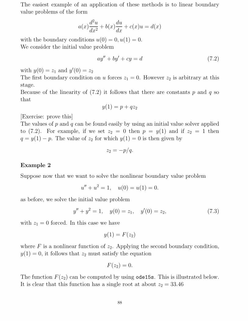
The function F (z2) can be computed by using ode15s. This is illustrated below.It is clear that this function has a single root at about z2 = 33.46
88
0 5 10 15 20 25 30 35 40 45 50−8
−6
−4
−2
0
2
4
6
root at 33.4618
z2
f
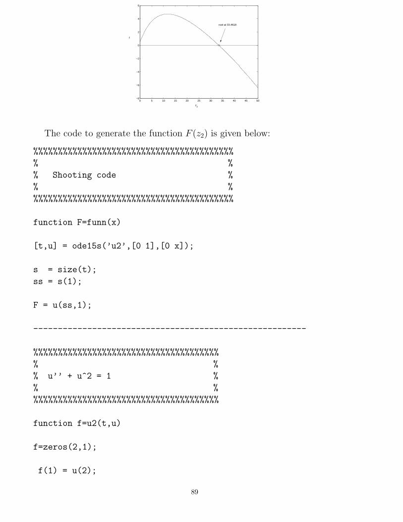
The code to generate the function F (z2) is given below:
%%%%%%%%%%%%%%%%%%%%%%%%%%%%%%%%%%%%%%%%%
% %
% Shooting code %
% %
%%%%%%%%%%%%%%%%%%%%%%%%%%%%%%%%%%%%%%%%%
function F=funn(x)
[t,u] = ode15s(’u2’,[0 1],[0 x]);
s = size(t);
ss = s(1);
F = u(ss,1);
--------------------------------------------------------
%%%%%%%%%%%%%%%%%%%%%%%%%%%%%%%%%%%%%%
% %
% u’’ + u^2 = 1 %
% %
%%%%%%%%%%%%%%%%%%%%%%%%%%%%%%%%%%%%%%
function f=u2(t,u)
f=zeros(2,1);
f(1) = u(2);
89

f(2) = 1-u(1)^2;
--------------------------------------------------------
One way to find z2 is to use the MATLAB command fzero given an initialguess of z2 = 30. Notice the way that this code uses the function funn computerd
using ode15s.
>> z2 = fzero(’funn’,30)
z2 =
33.4618
The resulting solution u and u′ is illustrated below:
0 0.1 0.2 0.3 0.4 0.5 0.6 0.7 0.8 0.9 1−40
−30
−20
−10
0
10
20
30
40
x
u
du/dx
An alternative method, which exploits the structure of the problem, is to use aNewton-Raphson method. As F (z2) = y(1) it follows that
dF
dz2=
dy(1)
dz2= φ(z2)
where the function φ(x) satisfies the variational equation
φ′′ + 2yφ = 0, φ(0) = 0, φ′(0) = 1.
To use this method we take a guess z(n)2 for z2 and then simultaneously solve the
two ODES
y′′ + y2 = 1, y(0) = 0, y′(0) = z(n)2 , φ′′ + 2yφ = 0, φ(0) = 0, φ′(0) = 1,
using ode15s. We then use a Newton-Raphson iteration to improve the guessvia the equation
z(n+1)2 = z
(n)2 −
y(1)
φ(1).
This procedure converges rapidly given a reasonable starting guess.
90

7.3 Finite Difference Methods
7.3.1 Discretising the second derivative.
Finite difference methods aim to to find the solution at all interior points withinthe interval [a, b]. Suppose that we divide up the interval [a, b] into N equal
divisions, so that if h = (b − a)/(N − 1) we set xi = a + (i − 1)h i = 1, . . . , N.Now we introduce a vector Ui so that
Ui ≈ u(xi) (7.4)
Now, by using a Taylor series expansion, it follows that
u(xi+1) = u(xi) + hu′(xi) + h2
2 u′′(xi) + . . .
u(xi−1) = u(xi) − hu′(xi) + h2
2 u′′(xi) + . . .
By making a slightly more detailed calculation it follows that
u(xi+1) − 2u(xi) + u(xi−1)
h2= u′′(xi) +
h2
12uiv(xi) + . . . (7.5)
We now can use (7.5) to approximate u′′ by
u′′ ≈Ui+1 − 2Ui + Ui−1
h2≡
δ2
h2Ui (7.6)
where δ2 is the iterated central difference operator. The leading error made in(7.6) when approximating u′′ by the iterated central difference is then propor-
tional to h2uiv. Now suppose that A is the tri-diagonal matrix given by
A =
1 0 . . . 01/h2 −2/h2 1/h2
. . . . . . . . .
1/h2 −2/h2 1/h2
0 1
,
If the vector U then satisfies the linear system
AU =
αf2...
fN−1
β
where fi ≡ f(xi) (7.7)
then (7.7) is a discretisation to the second order BVP with Dirichlet boundary
conditions which is given by
u′′ = f(x), u(a) = α, u(b) = β.
91

If we replace U by u in (7.7) the expression (7.5) implies that we would makean error of order h2 as h → 0. Note that the structure of A forces U1 = α andUN = β. The vector U can then be found via the operation
U = A−1
αf2
fN−1
β
Provided that the problem is not too irregular it can then be shown that in thelimit of N → ∞ (h → 0) we have
Ui = u(xi) + O(h2) as h → 0.
The solution of the BVP thus becomes (under discretisation) the problem of
solving the linear system (7.7).If f = [α, f2, . . . , fN−1, β]′ then this can be done in MATLAB via the command
A\f .
Whilst this is simple to use it is not especially efficient as the backslash operatordoes not exploit the special tri-diagonal structure of Matrix A. A much more
efficient algorithm of complexity O(N) is the Thomas algorithm which exploitsthis structure and is based on the LU decomposition. This algorithm is described
in Assignment 4. (Note, use of the MATLAB sparse matrix routines will speedthings up here.)
Efficiency is important as the relatively large error of O(N−2) in this methodmeans that we have to take a large value of N to get a reasonable error estimate.
More careful discretisations lead to smaller errors at the expense of more work.
7.3.2 Different boundary conditions
We can extend this idea to BVPs with Neumann boundary conditions. Forexample the BVP u′′ = f with the boundary conditions
u′(a) = α, u(b) = β.
Problems such as this arise frequently in models of heat conduction and electricalflow. For example, the boundary condition u′(a) = 0 corresponds to a thermal or
electrical insulator. There are many ways to deal with such a derivative boundarycondition. In the simplest we approximate
u′(a) by (U2 − U1)/h (7.8)
92

This will change the matrix A to the tridiagonal matrix
A ≡
−1/h 1/h 0 . . . 0
1/h2 −2/h2 1/h2
. . . . . . . . .
1/h2 −2/h2 −1/h2
0 0 1
and we must consider the solution to the linear system:
AU =
αf2...
fN−1
β
(7.9)
The linear equation (7.9) is then a discretisation of the BVP
u′′ = f u′(a) = α, u(b) = β.
The expression (7.8) is only accurate to O(h) as an approximation to u′(a). Wecan improve this by using the approximation
u′(a) ≈ (4U2 − U3 − 3U1)/2h
Exercise. Show that this expression is accurate to O(h2)
This leads to a slightly different matrix A. Unfortunately the resulting matrix isno longer tri-diagonal and we cannot use the Thomas algorithm to invert it.
A special case of Neumann boundary conditions arises when u′(a) = 0. In thiscase we can introduce a “ghost” point U0 approximating u(a−h). The boundarycondition implies that to 0(h3) we have U0 = U2. At the point x = 0 we have
u′′(a) ≈U0 + U2 − 2U1
h2=
2U2 − 2U1
h2(7.10)
This approximation to u′′(a) is correct to O(h2). (Can you show this?)
The resulting matrix A is then given by
A =1
h2
−2 2
1 −2 11 −2 1
. . . . . .
Note that in this case A is tri-diagonal, and we can again solve the linear systemby using the Thomas algorithm.
93

%%%%%%%%%%%%%%%%%%%%%%%%%%%%%%%%%%%%%%%%%%%%%%%%%%%%%%%%%%%%
% %
% Code to solve the Neumann two-point boundary value %
% problem: %
% %
% u’’ = -exp(x), u’(0) = 0, u(1) = 0. %
% %
%%%%%%%%%%%%%%%%%%%%%%%%%%%%%%%%%%%%%%%%%%%%%%%%%%%%%%%%%%%%
%
% Set up the mesh
%
N = 101;
h = 1/(N-1);
x = [0:h:1];
%
% Set up the matrix
%
A = diag(ones(N-1,1),-1) + diag(ones(N-1,1),1) - 2*diag(ones(N,1));
A = A/h^2;
%
% Neumann boundary condition at x = 0
%
A(1,2) = 2/h^2;
%
% Dirichlet boundary condition at x = 1
%
94

A(N,N-1) = 0;
A(N,N) = 1;
%
% Set up the right hand side
%
f = -exp(x)’;
%
% Modify this to allow for the Dirichlet boundary condition
%
f(N) = 0;
%
% Solve the system (without using the Thomas algorithm)
%
U = A\f;
%
% Plot the solution
%
plot(x,U)
0 0.1 0.2 0.3 0.4 0.5 0.6 0.7 0.8 0.9 10
0.1
0.2
0.3
0.4
0.5
0.6
0.7
0.8
0.9
x
U(x) Neumann condition
Dirichlet condition
95

A second example of differential equations occurs for BVPs with periodic bound-ary conditions for which u(a) = u(b) and u′(a) = u′(b). Periodic boundaryconditions often arise when looking at those BVPs that describe the travelling
wave solutions of hyperbolic equations. They also arise naturally when solvingBVPs on circles or spheres. A natural example of the latter being weather fore-
casting on the whole globe. Often BVPs with periodic boundary conditions aresolved using spectral methods in which the solution is expressed as a combina-
tion of trigonometric functions. However they can also be solved by using finitedifference methods. Exploiting periodicity we have
u′′(a) ≈u(a + h) + u(a − h) − 2u(a)
h2=
u(a + h) + u(b − h) − 2u(a)
h2(7.11)
which we approximate by
u′′(a) ≈U2 + UN−1 − 2U1
h2
Setting U = [U1, . . . , UN−1]′ (noting that U1 = UN) the resulting matrix A is
given by
A =
−2/h2 1/h2 0 . . . 0 1/h2
1/h2 . . . . . . 0
0 . . . . . .
1/h2 . . . . . . 1/h2 −2/h2
The resulting discretisation of u′′ then has an error of O(h2) as before. Thematrix A is not tri-diagonal, but its special periodic structure means that it canbe inverted quickly by using the FFT.
7.3.3 Adding in convective terms
In many applications we meet convection- diffusion problems which typicallytake the form
ǫu′′ + u′ = f with ǫ small.
These arise in fluid mechanics problems, where ǫ is a measure of the viscosity of
the fluid. The most accurate discretisation of u′ is given by the central differencediscretisation
u′ ≈δU
2h≡
Ui+1 − Ui−1
2h
A simple calculation shows that the central difference gives an error O(h2) whenapproximating u′.
However this discretisation of u′ leads to problems. In particular A−1 may benearly singular and ill-conditioned. If ǫ is zero then A has an eigenvector of the
96

form e = (1,−1, 1,−1, 1,−1, . . .) with zero eigenvalue eigenvalue. Check thissothat A−1 is singular.For small ǫ, A continues to have a similar eigenvector to ǫ with a small eigenvalue.
When inverting A the contribution of e to the solution is greatly amplified, andcan lead to an oscillatory contribution to the solution. This instability is BAD
but can easily be detected as it is on a grid scale. i.e all oscillations in the solutionare the same size as the mesh.
Oscillations can be avoided by taking h small enough to avoid this instability sothat
h ≤ 2ǫ
However, this is a very restrictive condition if ǫ is small.
One way to avoid the instability when ǫ > 0 is to replace u′ by its upwinddifference
Ui+1 − Ui
h
This is a less accurate approximation of u′ than the central differenceas
Ui+1 − Ui
h2= u′ + O(h)
However the resulting matrix A is much better conditioned and inverting it does
not lead to spurious oscillations in the solution What this approximation is doingis to exploit a natural flow of information in the system.
This is not always a good solution as often we can’t tell in advance if we needto use the upwind difference or the downwind difference Ui−Ui−1
h . However, like a
stiff solver, the use of the upwind difference allows us to use a step size governedby accuracy rather than stability. An example of the effect of using these differ-ent discretisations is given in Assignment 4.
7.4 Nonlinear Problems.
So far we have looked at linear two point BVPs. However,
MOST PROBLEMS ARE NONLINEAR
97

An important class of nonlinear two point BVPs (called semilinear problems)take the form
a(x)u′′ + b(x)u′ + f(x, u) = 0, (7.12)
and we need to develop techniques to solve them. Two examples of such problemsare given by the differential equation
u′′ + eu/(1+u) = 0, u(a) = u(b) = 0
which models combustion in a chemically reacting material, and
u′′ +2
xu′ + k(x)u5 = 0, u′(0) = 0, u(∞) = 0, u > 0,
which describes the curvature of space by a spherical body.
A special case is given by the equation
u′′ + f(u) = 0, u(a) = α, u(b) = β. (7.13)
Discretising the differential equation (7.13) leads to a set of nonlinear equations
of the formAU + f(U) = 0 (7.14)
where A is the matrix given earlier and the vector f is given by
fi ≡ f(Ui).
As with most nonlinear problems, we solve this system by iteration starting
with an initial guess although, be warned, the system may have one, none ormany solutions. Perhaps the most effective such method is the Newton-Raphsonalgorithm. Suppose that U (n) is an approximate solution of (7.14), we define the
residual R(n) byAU (n) + f(U (n)) = R(n). (7.15)
The size of Rn is a measure of the quality of this solution.
Now if we define the Jacobian of the nonlinear function f by
Jij = ∂fi/∂Uj
the “linearisation” L of (7.15) acting on a vector ϕ is given by
Lϕ ≡ Aϕ + Jϕ.
The Newton-Raphson iteration updates U (n) to U (n+1) via the iteration
U (n+1) = U (n) − L−1R(n)
98

Here the vector W ≡ L−1R(n) can be found by solving the linear system
AW + JW = R(n).
This algorithm converges rapidly (often in about 5 iterations) if the initial guess
U (0) is close to the true solution. Finding such an initial guess can be difficultfor a general problem and often requires some a-priori knowledge of the solution.
The Fortran code AUTO uses the Newton-Raphson method coupled to a path-following (homotopy) method to find the solution of a version of the nonlinear
systems arising from discretisations of nonlinear BVPs obtained by using collo-cation.
7.5 Other methods
At present collocation is the best method for solving 2pt BVPs. This is a bit likethe Finite difference method but uses much higher order polynominals. It is alsoclosely related to implicit Runge-Kutta methods. However, the collation method
has no easy extension to higher dimensions. In higher dimensions two-pointBVPs generalise to elliptic partial differential equations. For such problems the
finite element method is the mainly used solution procedure, although spectralmethods are widely used for problems with a relatively simple geometry e.g.
weather forecasting on the sphere.
Melina Freitag 2007
99