1

TOPOLOGY

M.A. Mathematics (Previous)PAPER-III

Directorate of Distance EducationMaharshi Dayanand University

ROHTAK – 124 001

2

Copyright © 2003, Maharshi Dayanand University, ROHTAKAll Rights Reserved. No part of this publication may be reproduced or stored in a retrieval system or trans-

mitted in any form or by any means; electronic, mechanical, photocopying, recording or otherwise, without thewritten permission of the copyright holder.

Maharshi Dayanand UniversityROHTAK – 124 001

Developed & Produced by EXCEL BOOKS PVT. LTD., A-45 Naraina, Phase 1, New Delhi-110028

3

Contents

Chapter 1 Toplogical Spaces 5

Chapter 2 Connectedness 30

Chapter 3 Compactness and Continuous Functions 38

Chapter 4 Separation Axiom (I) and Countability Axioms 49

Chapter 5 Separation Axiom (Part II) 63

Chapter 6 Embedding and Metrization 81

Chapter 7 Product Topological Spaces 87

Chapter 8 Nets & Filters 98

Chapter 9 The Fundamental Group and Covering Spaces 118

Chapter 10 Paracompact Spaces 143

4

M.A. (Previous)TOPOLOGY

Paper-III M.Marks: 100Time: 3 Hrs.

Note: Question paper will consist of three sections. Section-I consisting of one question with ten parts of2 marks each covering whole of the syllabus shall be compulsory. From Section-II, 10 questions to be setselecting two questions from each unit. The candidate will be required to attempt any seven questionseach of five marks. Section-III, five questions to be set, one from each unit. The candidate will be re-quired to attempt any three questions each of fifteen marks.

Unit-I

Definition and examples of topological spaces, closed sets and closure, dense subsets. Neighbourhoods interiorExterior and boundary operations, Accumulation points and Derived sets. Bases and subbase. Subspaces andrelative topology. Alternative method of defining a topology in terms of Kuratowski closure operator andneighbourhood systems. Continuous functions and homoemorphisms.

Connected spaces. Connectedness on the real time. Components, Locally connected spaces.

Unit-II

Compactness, continuous functions and compact sets. Basic properties of compactness and finite intersectionproperty. Sequentially and countably compact sets, Local compactness and one point compactification.

Separation axioms T0, T1 and T2 spaces, Their characterization and basic properties, Convergence on T0 space.Firstand second countable spaces, Lindelof’s Theorems, Separable spaces and separability.

Unit-III

Regular and normal spaces, Urysohn’s Lemma and Tietze Extension Theorem, T3 and T4 spaces, Completeregularity and complete normality, T3/½ and T5 spaces.

Embedding and Metrization. Embedding Lemma and Tychonoff embedding Urysohn’s Metrization Theorem.

Unit-IV

Product topological spaces, Projection mapppings, Tychonoff product topology in terms of standard subbasesand its characterization, Separation axioms and product spaces, Connectedness, locally connectedness and Com-pactness of product spaces. Product space as first axiom space.

Nets and filters. Topology and convergence of nets. Hausdorffness and nets. Compactness and nets. Filters andtheir convergence. Canonical way of converting nets to filters and vice-versa. ultra filters and compactness.Stone-Cech compactification.

Unit-V

Homotopy of paths, Fundamental group, Covering spaces, The fundamental group of the circle and fundamentaltheorem of algebra.

Covering of a space, local finiteness, paracompact spaces, Michaell theorem on characterization of paracompactnessin regular space, Paracompactness as normal, Nagata-Smirnov Metrization theorem.

TOPOLOGY 5

TOPOLOGY The word topology is derived from two Greek words, topos meaning surface and logs meaning discourse or study. Topology thus literally means the study of surfaces or the science of position. The subject of topology can now be defined as the study of all topological properties of topological spaces. A topological property is a property which if possessed by a topological space X, is also possessed by every homeomorphic image of X. If very roughly, we think of a topological space as a general type of geometric configuration, say, a diagram drawn on a sheet of rubber, then a homemorphism may be thought of as any deformation of this diagram (by stretching bending etc.) which does not tear the sheet. A circle can be deformed in this way into an ellipse, a triangle, or a square but not into a figure eight, a horse shoe or a single point. Thus a topological property would then be any property of the diagram which is invariant under (or unchanged by) such a deformation. Distances, angles and the like are not topological properties because they can be altered by suitable non-tearing deformations. Due to these reasons, topology is often described to non-mathematicians as “rubber sheet geometry”.

Maurice Frechet (1878-1973) was the first to extend topological considerations beyond Euclidean spaces. He introduced metric spaces in 1906 in a context that permitted one to consider abstract objects and not just real numbers or n-tupls of real numbers. Topology emerged as a coherent discipline in 1914 when Felix Hausdorff (1868-1942) published his classic treatise Grundzuge der Mengenlehre. Hausdorff defined a topological space in terms of neighbourhoods of member sof a set.

TOPOLOGICAL SPACES

6

1

TOPOLOGICAL SPACES

We begin with the study of topology with a brief motivational introduction to metric spaces. The ideas of metric and metric spaces are abstractions of the concept of distance in Euclidean space. These abstractions are fundamental and useful in all branches of mathematics. Definition. A metric on a set X is a function d : X×X→R that satisfies the following conditions. (a) d(x, y) ≥ 0 for all x, y ∈X (b) d(x, y) = 0 if and only if x = y (c) d(x, y) = d (y, x) for all x, y ∈ X. (d) d(x, z) ≤ d(x, y) + d(y, z) for all x, y, z ∈X. If d is a metric on a set X, ordered pair (X, d) is called a metric space and if x, y∈X, Then d(x, y) is the distance from x to y.

Metric Space

Note that a metric space is simply a set together with a distance function on the set.

The function d : R×R→R defined by d(x, y) = |x−y| satisfies the four conditions of the definition and hence this function is a metric on R. It is called the usual metric on R. Also the function d : R2

× R2→R defined by d(x1 x2), (y1, y2) = 221

221 )yy()xx( −+− is called the usual metric on R2.

Definition. A subset U of a metric space (X, D) is open if for each x ∈ U, there is an open ball Bd(x, ∈) such that Bd(x, ∈) ⊆ U. The open subsets of a metric space (X, d) have the following properties. (a) X and φ are open sets (b) The union of any collection of open sets is open. (c) The intersection of any finite collection of open sets is open.

Metrizable

A metrizable space is a topological space X with the property that there exists at least one metric on the set X whose class of generated open sets is precisely the given topology i.e. it is a topological space whose topology is generated by some metric. But metric space is a set with a metric on it. The following example shows that there are topological spaces that are not metrizable. Example. Let X be a set with at least two members and T be the trivial topology on X, then (X, T) is not metrizable.

Definition and examples of Topological spaces

Definition. A topological space is a pair (X, T) consisting of a set X and a family T of subsets of X satisfying the following axioms : (01) φ, X∈T (02) The intersection of any finite number of sets in T is in T.

TOPOLOGY 7

(03) Any union (countable or not) of sets in T is in T. The set X will be called a space, its elements points of the space and the subsets of X belonging to the family T, sets open in the space. The collection T is called a topology for X.

Axioms (01)→(03) of the family of open sets can be formulated in the following manner (01) The empty set and the whole space are open (02) The intersection of two open sets is open (03) The union of arbitrary many open sets is an open set.

Examples of Topological Spaces

1. Example. Let X a, b, c, d, e. Consider the following classes of subsets of X . S1 = φ, X, a, c, d a, c, d, b c, d e S2 = φ, X, a, c, d, a, c, d, b, c, d

S3 = φ, X, a, c, d, a, c, d, a, b, d, e We observe that S, is a topology on X since it satisfies the three axioms.

But S2 is not a topology on X since the union a, c, d ∪ b, c, d = a, b, c, d of two members of S2 is not in S2 and so S2 does not satisfy the third axiom.

Similarly it can be seen that S3 is not a topology on X since the intersection

a, c, d ∩ a, b, d, e = a, d

of two sets in S3 does not belong to S3 and so S3 does not satisfy the second axiom

2. Example. A metric space is a special kind of topological space. The open sets being defined as usual the axioms (01) − (03) hold since

(01) φ and X in a metric space (X, d) are open. (02) The intersection of any finite number of open sets in (X, d) is open. (03) Any union (countable or not) of open sets in (X, d) is open. This topology defined on metric space is called usual topology on a metric space.

3. Example. Let D denote the class of all subsets of X. Then D satisfies all axioms for a topology on X. This topology is called the Discrete topology and (X, D) is called a Discrete topological space or simply a Discrete Space.

4. Example. Let X be a nonempty set. The family I = φ, X consisting of φ and X is itself a topology on X and is called the Indiscrete topology or simply an Indiscrete space. It is the coarsest topology.

Remark. When X is a singleton, then the two topologies discrete and indiscrete coincide.

5. Example. Let X be any infinite set and T be the family consisting of φ and complements of finite subsets of X. Show that T is a topology on X.

Analysis. Let X be an infinite set and T be the family consisting of φ and subsets of X whose complements in X are finite.

To prove that T is a topology on X. (1) φ∈T and since φ is finite φC = X∈T (2) Let G1, G2 ∈T G1 ∩ G2 ∈T If G1 ∩ G2 = φ then G1 ∩ G2 ∈T If G1 ∩ G2 ≠ φ, then G1 ≠ φ, G2 ≠ φ and G1, G2∈T X−G1 and X−G2 are finite (X−G1) ∩ (X−G2) is finite

TOPOLOGICAL SPACES

8

X −(G1 ∩G2) is finite G1 ∩G2 ∈T Thus in either case G1, G2 ∈T G1 ∩G2 ∈T (3) Let Gα ∈ T X − Gα is finite

∩ (X −Gα) is finite

∩ GαC is finite

X − (

∩ GαC) ∈T

∪ (GαC)C ∈T

∪ Gα ∈T

Hence all the axioms for a topology are satisfied. T is a topology on X.

Remark. This topology is called cofinite topology.

6 Example. Let X be a set and T = ∪ ∈ P(X), ∪ = φ or X − ∪ is countable. Then T is a topology on X and is called the countable complement topology on X.

Remark. If X is a finite set, then the finite complement topology, the countable complement topology and the discrete topology are the same.

7. Example. Let T = B ∈ P(R); B is an interval of the form [a, b) Then T satisfies all the conditions for a topology. This topology is called lower limit topology on R.

8. Example. Let T B ∈ P(R); B is an interval of the form (a, b]

Then T satisfies all the conditions for a topology and this topology is called upper limit topology on R.

9. Example. Let X be a linearly ordered set. Then order topology for X is obtained by choosing as a subbase for all sets which are either of the form x, x > a or of the form x; x < a for some a∈X.

10. Example. Let X = 1,2,3 . List some of topologies on X. Are there any collection of subsets of X that are not topologies on X.

Solution. Of course we have the trivial topology and the discrete topology. We list some other topologies, T1 = φ, X, 1 T2 = φ, X, 1, 2 T3 = φ, X, 1, 2, 1, 2 T4 = 1, 2, 3, φ, X T5 = φ, X, 2, 1, 2, 2, 3 T6 = φ, X, 1, 1, 2, T7 = φ, X, 1, 2, 1, 2, 2, 3 There are collections of subsets of X = 1, 2, 3 that are not topologies on X. e.g. φ, X, 1, 2, 2, 3 and φ, X, 1, 2 .

TOPOLOGY 9

Theorem. 1. The intersection T1 ∩ T2 of any two topologies T1 and T2 on X is also a topology on X.

Proof. Since T1 and T2 are topologies on X, therefore φ, X ∈T and φ, X∈ T2 φ, X ∈T1 ∩T2 That is T1 ∩ T2 satisfies first axiom for a topology Also if G, H ∈ T1 ∩ T2, Then G, H ∈ T1 and G, H ∈ T2

Since T1 and T2 are topologies G ∩ H ∈ T1 and G ∩ H ∈ T2 G ∩ H ∈ T1 ∩ T2 i.e. T1 ∩ T2 satisfies the second axiom for a topology. Further, let Gα ∈ T1 ∩ T2 for every α ∈ S, where S is an arbitrary set

Then Gα ∈ T1 and Gα ∈ T2 for every α∈S. but T1 and T2 are topologies ∪α Gα ∈ T1 and ∪α Gα ∈ T2 ∪α Gα ∈ T1 ∩ T2. i.e. T1 ∩ T2 satisfies third axiom for a topology. Hence the result follows.

Remark. The union T1 ∪ T2 of two topologies on a set X need not be a topology on X for example, let X = a, b, c, then T1 = φ, X, a, b a, b T2 = φ, X, a, c, a, c are two topologies on X but T1 ∪ T2 = φ, X, a, b, c, a, b, a, c is not a topology on X since union of b and c is not in T1 ∪ T2

Definition. Let (X, T1) and (X, T2) be topological spaces with the same set X. Then T1 is said to be finer than T2 if T1 ⊃ T2. The topology T2 is then said to be coarser than T1. Clearly the discrete topology is the finest topology and the indiscrete topology is the coarset topology defined on a set.

Accumulation Points and Derived Sets.

Definition. Let (X, T) be a topological space and E ⊆ X. A point x is said to be a limit point or accumulation point of the set E if for every open set G containing x, we have E ∩G − x ≠ φ The set of all limit points of a set E is called the derived set of E and is denoted by d(E).

Example 1. Let (X, T) be a discrete topological space. Then each point is an open set and E ∩ x − x = φ and therefore the derived set of every set E is empty Example 2. Let (X, T) be an indiscrete topological space then the only open set containing a point x is X itself. Consider E ∩ X − x = E −x If E consists of two points, then E −x ≠ φ and therefore the derived set of any set containing at least two points is the entire space X. If E is empty, then the derived set of E is empty since φ ∩ X − x = φ If E consists of exactly one point, then the derived set of E is the complement of that point.

Example 3. Let X = a, b, c and T = φ, a, b, a, b, X

TOPOLOGICAL SPACES

10

Then we note that a is contained in a, a, b and X and a ∩ a − a = φ a ∩ a, b − a = φ a ∩ X − a = φ

This implies that a is not a limit point of a . Similarly b is not a limit point of a. Since X is the only open set containing c Hence a ∩ X − c ≠ φ This implies that c is a limit point of a

Remark. The definition of a limit point is equivalent to “A point x is said to be a limit point of E if every open set containing x contains a point of E different from x”.

Theorem 2. If A, B and E are subsets of the topological space (X, T), then the derived set has following properties. (i) d(φ) = φ (ii) If A ⊆ B, then d(A) ⊆ d(B) (iii) If x ∈ d(E), then x ∈d E −x (iv) d(A ∪ B) = d(A) ∪ d(B)

Proof. (i) holds since φ ∩ G − x = φ for any x ∈X and G ∈T. (ii) Since A ⊆ B A ∩ G − x ⊆ B ∩ G −x d(A) ⊆ d(B) This proves (ii) (iii) To prove (iii), we note that [E −x] ∩ G −x = [E ∩ xC] ∩ G ∩ xC

= E ∩ G ∩ [xC = E ∩ G −x Therefore if x ∈ d(E), then X ∈ d [E − x] (iv) Since A ⊆ A ∪ B and B ⊆ A ∪ B d(A) ⊆ d (A ∪ B) and d(B) ⊆ d(A ∪ B) d(A) ∪ d(B) ⊆ d(A ∪ B) Conversely suppose that x ∉ d(A) ∪ d(B) and so x ∉ d(A) and x ∉ d(B). Therefore by definition, there must exist GA and GB containing x such that GA ∩ A − x = φ GB ∩ B − x = φ Let G = GA ∩ BB. By axiom of topology, this is an open set since x ∈ GA, GB

x ∈ G. But G ∩ A −x = G ∩ B − x = φ and so G ∩ A ∪ B − x = φ x ∉ d(A ∪ B) d(A ∪ B) ⊆ d(A) ∪ d(B)

Closed Sets and Closure

The concept of a topological space has been introduced in terms of the axioms for the open sets. Similarly closed sets are used as the fundamental notion of topology.

Definition. Let (X, T) be a topological space. A set F ⊆ X is said to be closed if it contains all of its limit points. Thus F is closed iff d(F) ⊆ F.

TOPOLOGY 11

Theorem 3. If x ∉ F, where F is a closed subset of a topological space (X, T), then there exists an open set G such that x ∈ G ⊆ FC

Proof. Suppose no such open set exists. Then x ∈ G ∈ T would imply that G ∩ F ≠ φ.

Since x ∉ F, G ∩ F −x ≠ φ.

This implies that x is a limit point of F that is x ∈ d(F). F however is a closed set and so d(F) ⊆ F, so that x must belong to F. but this is contradiction to x ∉ F. This contradiction shows that such an open set must exist.

Cor. 1. If F is a closed set, then F is open.

Proof. If x ∈ FC, then x ∉ F where F is a closed set. By the above theorem, there exists an open set Gx such that x ∈ Gx ⊆ FC. But then FC = U x ; x ∈ FC ⊆ U Gx ; x ∈ FC ⊆ FC Thus FC = U Gx ; x ∈ FC which is the union of open sets and hence an open set.

Cor. 2. If FC is an open set, then F is closed.

Proof. Suppose x is a limit point of F and let x ∉ F. Then x ∈ FC, and F ∩ FC − x = φ which implies that x is not a limit point of F. Hence the assumption that x ∉ F is wrong. Therefore, every limit point of F is in F and so F is closed.

Remark. 1. From Cor 1 and Cor 2, it follows that “A set is a closed subset of a topological space if and only if its complement is an open subset of the plane.”

Remark. 2. From the De-Morgan’s Laws and from the three axioms of a topological space, the following properties of the closed set follows (c1) The empty set and the whole space are closed (c2) The union of two closed sets is closed. (c3) The intersection of arbitrary many closed sets is a closed set.

As an example, we give a proof for property (c2) and (c3). (c2) Suppose F and G are two closed sets then FC and GC are open since union of two open sets is open FC ∪ GC is open. (F ∩ G)C is open [by De-Morgan’s Law]

F ∩ G is closed Intersection of two closed sets is closed.

(c3) Let a family Fss∈S of closed sets be given. By definition the set Us = X − Fs is open for every s ∈ S. Since

Ss∈∩ Fs =

Ss∈∩ (X − Us) = X −

Ss∈∪ Us.

Since the set Ss∈

∪ Us is open, Ss∈

∩ Fs is a closed set.

Theorem. 4. If d(F) ⊆ A ⊆ F and F is a closed set, then A is closed.

TOPOLOGICAL SPACES

12

Proof. Since A ⊆ F d(A) ⊆ d(F)

But F is closed, hence d(A) ⊆ d(F) ⊆ A ⊆ F i.e. d(A) ⊆ A which implies that A is closed.

Cor. The derived set of a closed set is closed.

Proof. Let F be a closed set we have to prove that d(F) is closed. Now as F is closed, d(F) ⊆ F

d(d(F)) ⊆ d(F) ⊆ F . Thus by the above theorem, d(F) is closed.

Definition. Let (X, T) be a topological space and E ⊆ X. Then closure of E denoted by C(E) is defined by C(E) = ∩ all closed sets containing E

Since by (c1), the family of closed sets containing E is non-void and by (c3), the intersection of all elements of this family is closed. Hence closure of a set is closed and it is the smallest closed set containing E.

Theorem. 5. For any set E in a topological space, C (E) = E ∪ d(E)

Proof. Suppose x ∉ E ∪d(E), so that x ∉ E and x ∉ d(E), there exists an open set Gx containing x such that E ∩ Gx − x = φ

Since x ∉E, this actually means that E ∩ Gx = φ so Gx ⊆ EC. Since Gx is open set disjoint from E, no point of Gx can be a limit point of E, that is Gx ⊆ (d(E))C, Thus [E ∪ d(E)]C= ∪ Gx; x ∉ E ∪ d(E) which is an open set since arbitrary union of open sets is open. Therefore E ∪ d(E) is closed, which obviously contains E. Hence C(E) being the smallest closed set containing E, we have C(E) ⊆ E ∪ d(E).

Conversely suppose that x ∈ E ∪ d(E) and suppose that F is any closed set containing E. If x ∈ d(E), then x ∈ d(F) and so x ∈ F [since d(E) ⊆ d(F) ⊆ F]. But if x ∈ E, then again we have x ∈ F since E ⊆ F, Thus x belongs to any closed set containing E and hence to the intersection of all such sets, which is the closure of E. Thus E ∪ d(E) ⊆ C(E).

Hence C(E) = E ∪ d(E)

Remark. For arbitrary subsets A and B of the space X if A ⊂ B, then C(A) ⊂ C(B). Indeed if A ⊆ B, then the family of closed sets containing A is contained in the family of closed sets containing B, then C(A) ⊆ C(B).

Theorem. 6. E is closed if and only of E = C(E)

Proof. We suppose first that E is closed Then d(E) ⊆ E. Since C(E) = E ∪ d(E), therefore it follows that if E is closed, then C(E) = E ∪ d(E) = E Conversely if E = C(E), then C(E) being the intersection of all closed sets containing E is closed. Hence E is closed

Kurtowski Closure Axioms

Definition. An operator C of ρ(X) into itself which satisfies the following four properties (known as Kuratowski closure axioms) is called a closure operator on the set X.

TOPOLOGY 13

Theorem. 7. In the topological space (X, T), the closure operator has the following properties. (K1) C(φ) = φ (K2) E ⊆ C(E) (K3) C(C(E)) = C(E) and (K4) C (A ∪ B) = C(A) ∪ C(B)

Proof. (K1) Because the void set is closed and also we know that a set A is closed if and only if A = C(A), therefore it follows that C(φ) = φ. (K2) It follows from the definition as C(E) is the smallest closed set containing E (K3) Since C (E) is the smallest closed set containing E, we have C(C(E)) = C(E) by the result that a set is closed if and only if it is equal to its closure (K4) Since A ⊂ A ∪ B and B ⊂ A ∪ B, therefore C(A) ⊂ C(A ∪ B) and C(B) ⊂ C(A ∪ B) and so C(A) ∪ C(B) ⊂ C(A ∪ B) (1) By (K2), we have

A ⊂ C(A) and B ⊂ C(B) Therefore A ∪ B ⊂ C(A) ∪ C(B)

Since C(A) and C(B) are closed sets and so C(A) ∪ C(B) is closed. By the definition of closure, we have C(A ∪ B) ⊂ C [C(A) ∪ C(B)] (2) From (1) and (2), we have C(A ∪ B) = C(A) ∪ C(B).

Remark. C(A ∩ B) may not be equal to C(A) ∩ C(B). e.g. if A = (0, 1), B = (1, 2), then C(A) = [0, 1], C(B) = [1, 2]

Therefore, C(A) ∩ C(B) = 1 where A ∩ B = φ But C(φ) = φ. Therefore C(A ∩ B) = φ and thus C(A ∩ B) ≠ C(A) ∩ C(B)

Remark. The closure operator completely determines a topology for a set A is closed iff A = C(A). In other words the closed sets are simply the sets which are fixed under the closure operator. We shall prove it in the form of the following.

Defining Topology in Terms of Kuratowski Closure Operator

Theorem. 8. Let C* be a closure operator defined on a set X. Let F be the family of all subsets F of X for which C*(F) = F and let T be a family of all complements of members of F . Then T is a topology for X and if C is the closure operator defined by the topology T. Then C*(E) = C(E) for all subsets E ⊆ X.

Proof. Suppose Gλ ∈ T for all λ. We must show that

∪ Gλ ∈ T i.e. (

∪ Gλ)C∈ F.

Thus we must show that C* [(

∪ Gλ)C] = (

∪ Gλ)C

By (K2) (

∪ Gλ)C ⊆ C*[(

∪ Gλ)C]

so we need only to prove that C* [(

∪ Gλ)C] ⊆ (

∪ Gλ)C

By De-Morgan’s Law, this reduces to C* [

∩ (Gλ)C] ⊆

∩ (Gλ)C

TOPOLOGICAL SPACES

14

Since (

∩ (Gλ)C ) ⊆ (Gλ)C) for each particular λ.

C*[

∩ (Gλ)C] ⊆ C*[(Gλ)C] for each λ and

so C*[

∩ (Gλ)C] ⊆

∩ C*[(Gλ)C] (1)

But Gλ ∈ T (Gλ)C ∈ F, so C*[(Gλ)C] = (Gλ)C Thus we have from (1) C*[

∩ (Gλ)C] ⊆

∩ (Gλ)C

Hence if Gλ ∈ T, then

∪ Gλ ∈ T

To check that φ, X ∈ T, we observe that by Kuratowaksi closure axiom (K2) X ⊆ C*(X) ⊆ X C*(X) = X X ∈ F Hence XC = φ ∈ T. Also by (Kurtowaski closure axiom K1), we have C*(φ) = φ φ ∈ F φC = X ∈ T. Finally suppose that G1 G2 ∈ T. Then by hypothesis C*(G1)C = G1

C and C*(G2)C = G2C.

We may now calculate that C* [(G1 ∩ G2)C] = C*[ G1

C ∪ G2C]

= C(G1C) ∪ C*(G2

C) = G1

C ∪ G2C = (G1 ∩ G2)C

(G1 ∩ G2)C ∈ F G1 ∩ G2 ∈ T. Hence all the axioms for a topology are satisfied and hence T is a topology. We now prove that C* = C.

We have shown above that T is a topology for X. Thus members of T are open sets therefore the closed sets are just the members of the family F.

By (K3), C*[C*(E)] = C*(E) which implies that C*(E) ∈ F. Now by (K2) E ⊆ C*(E). Thus C*(E) is a closed set containing E and hence C*(E) ⊇ C(E) (1) as C (E) is the smallest closed set containing E. On the other hand by (K2) E ⊆ C(E) ∈ F so C*(E) ⊆ C*(C(E)) = C(E) (2) Thus by (1) and (2), C*(E) = C(E) for any subset E ⊆ X

Dense Subsets

Definition. Let A be a subset of the topological space (X, T). Then A is said to be dense in X if A = X.

Trivially the entire set X is always dense in itself. Q is dense in R since Q = R.

Let T be finite complement topology on R. Then every infinite subset is dense in R.

Theorem. 9. A subset A of topological space (X, T) is dense in X iff for every nonempty open subset B of X, A ∩ B ≠ φ.

TOPOLOGY 15

Proof. Suppose A is dense in X and B is a non empty open set in X. If A ∩ B = φ, then A ⊂ X − B implies that A ⊂ X − B since X − B is closed. But then X − B

≠⊂ X contradicting that A = X

[since A ⊂ X − B ≠⊂ X]

Conversely assume that A meets every non-empty open subset of X. Thus the only closed set containing A is X and consequently A = X. Hence A is dense in X.

Theorem. 10. In a topological space (X, T) (i) Any set C, containing a dense set D, is a dense set. (ii) If A is a dense set, and B is dense on A, then B is also a dense set.

Proof. (1) Since D ⊂ C D ⊂C But D = X hence X ⊂C also C ⊂ X so that C = X. Thus C is dense in (X, T) (iii) Since A is dense, A = X Also B is dense on A

A ⊂B A ⊂ B =B (By closure property) A ⊂B X =A ⊂B Thus B is dense in (X, T).

1.5. Neighbourhood

Definition. Let (X, T) be a topological space and let x be a point of X. Then a subset N of X is said to be a T-nbd of x if there exists a T-open set G such that x ∈ G ⊆ N. That is a nbd of a point is any set which contains an open set containing the point.

Remark.(i) It is evident from the definition that a T-open set is a T-nbd of each of its points but a T-nbd of a point need not be T-open. Also every open set containing x is a nbd of x we shall call such a nbd an open nbd of x (ii) Clearly E is a nbd of x if and only if x ∈ i(E)

Example. 1. Let X = 1, 2, 3, 4, 5 and T = φ, X 1, 1, 2, 1, 2, 3 1, 2, 4, 1, 2, 3, 4 is a topology on X.

For such a topological space all subsets containing 1 will be nbds of 1.

Example. 2. Let (X, D) be a discrete topological space and x ∈ X. In such a case all possible subsets of X will be nbd of x because here each subset of X is open. (3) If (X, I) is an indiscrete topological space, then X is the nbd of each of its points. Theorem 11. Let (X, T) be a topological space and A ⊂ X. Then A is open if and only if it contains nbd of each of its points.

Proof. Let A be an open set and x ∈ A be an arbitrary element. Since A is an open set such that x ∈ A ⊆ A, therefore A is a nbd of x. Thus A contains a nbd (namely A) of each of its points.

Conversely, let A contains a nbd of each of its points. So there exists a nbd Na for each a ∈ A such that Na ⊂ A. Therefore by definition of nbd, there exists an open set Sa such that a ∈ Sa ⊆ Na. Define S = ∪Sa ; a ∈ A

TOPOLOGICAL SPACES

16

We shall show that S = A and then clearly A will be open. If x ∈ A, then by the definition of Sx x ∈ Sx and so x ∈ ∪ Sa ; a ∈ A A ⊆ ∪ Sa ; a ∈ A A ⊆ S. (1) Also if y ∈ S, then y ∈ Sa for some a ∈ A. But Sa ⊂ Na ⊂ A Therefore y ∈ A which implies that S = ∪ Sa ; a ∈ A ⊂ A (2) (1) and (2) yield S = A Thus A is open.

Properties of Neighbourhood

Theorem. 12. Prove that

(N1) Every point of X is contained in at least one neighbourhood and is contained in each of its nbds. (N2) The intersection of any two nbds of a point is a nbd of that point. (N3) Any set which contains a nbd of a point is itself a nbd of that point. (N4) If N is a nbd of a point x, then there exists a nbd N* of x such that N is a nbd of each point of N*.

Proof. (N1) Since X is T-open, it is a T-nbd of every point. Hence there exists at least one T-nbd (namely X) for each x ∈ X. (N2) Let N and M be two neighbourhoods of x ∈ X. Then by definition, there exists open set G1 and G2 in X such that x ∈ G1 ⊂ N, x ∈ G2 ⊂ M which imply that x ∈ G1 ∩ G2 ⊂ N ∩M, where G1 ∩ G2 is open Hence N ∩ M is a nbd of x. (N3) Let N be any nbd of x in X and M be a set in X which contains N. By the definition of nbd, there exists an open set G of x such that x ∈ G ⊆ N But N ⊂ M, it follows that x ∈ G ⊆ N ⊂ M x ∈ G ⊂ M. Hence M is a nbd of x in X. (N4) Since N is a nbd of x. Therefore there exists an open set N* such that x N* ∈ N. Since N* is open, it is a nbd of each of its points. But N* ⊂ N, thus by (N3) N is a nbd of each of points of N*. Alternating Method of defining a topology in terms of neighbourhood system

Theorem. 13. Let there be associated with each point x of a set X, a collection Nx* of subsets called nbds subject to the above four properties. Let T be the family of all subsets of X which are nbds of each of their points i.e. G ∈ T iff x ∈ G implies that G ∈ Nx*. Then T is a topology for X and if Nx is the collection of all nbds of x defined by the topology T, then Nx* = Nx for every x ∈ X.

Proof. First we prove that T is a topology for X

TOPOLOGY 17

(01) of course φ ∈ T since it is a nbd of each of its points.

We also note that for any x ∈ X, x is contained in at atleast one nbd by (N1) and this nbd is contained in X, so X is a nbd of x by (N3). Thus X is a nbd of each of its points and so X ∈ T.

(02) Suppose G1 and G2 belong to T. If x ∈ G1 ∩ G2, then x ∈ G1 and x ∈ G2. By the definition of T, G1 and G2 are both nbds of each of their points. So G1 ∈ Nx*, G2 ∈ Nx*. Now by the property (N2) of nbd G1 ∩ G2 ∈ Nx* so G1 ∩ G2 is a nbd of each of its points.

(03) Suppose Gλ ∈ T for all λ. If x ∈

∪ Gλ, then x ∈ Gλ for some λ. Now by the definition of T,

Gλ is a nbd of each of its points, so Gλ ∈ Nx*, By (N3) property of nbd, since Gλ ⊆

∪ Gλ we have

∪ Gλ ∈ Nx*. Thus

∪ Gλ is a nbd of each of its points and hence belongs to T.

Thus T is a topology. IInd Part. To prove Nx* = Nx

If N ∈ Nx, then ∃ an open set G such that x ∈ G ⊆ N, from the definition of T, x ∈ G implies that G ∈ Nx* and so N ∈ Nx* by (N3) property of nbd.

Thus Nx ⊆ Nx* (1)

Now suppose N ∈ Nx*. Let us define the set G to be all points which have N as a nbd. Clearly x is one of these points and so x ∈ G. While by property (N1) of nbd, every point with N as a nbd is in N. So G ⊆ N. We shall show that G ∈ T that is G is in Ny* for every y ∈ G. Let y ∈ G, so that N ∈ Ny*. By (N4), there exists a set N* s that N*∈ Ny* such and if z ∈ N*, then N ∈ Nz* and the definition of G shows that N ∈ Nz* implies that z ∈ G, hence N* ⊆ G by (N3), G ∈ Ny* G ∈ T N is a nbd of x i.e. N ∈ Nx Nx* ⊆ Nx (2) [since N ∈ Nx*] .

From (1) and (2) Nx = Nx*

1.6. Interior, Exterior and Boundary Operators

Definition. The interior of a set E is the largest open set contained in E or equivalently the union of all open sets contained in E called the interior of the set E. The interior of the set E is denoted by i (E). The points of i(E) of E are known as interior points of E. A set E is open if and only if E = i(E)

Theorem. 14. For any set E in a topological space (X, T), i(E) = [C(EC)]C

Proof. Let x ∈ i(E), then i(E) is itself an open set containing x which is disjoint from E and so x ∉ d(EC). But x ∈ EC, x ∉d(EC). This implies that x ∉ EC ∪ d(EC) x∉C(EC) x ∈[C(EC)]C i(E) ⊆ [C(EC)]C Conversely suppose that x∈ [C(EC)]C

x ∉C(EC)

TOPOLOGICAL SPACES

18

x ∉ [EC ∪ d(EC)] x ∉ EC and x ∉ d(EC)

Thus x ∈ E and x is not a limit point of EC.

Thus there exists an open set G containing x such that EC ∩ G −x = φ Since x ∉ EC, we have EC ∩ G = φ and so G ⊆ E.

Thus x ∈ G ⊆ E for some open set G and so x belongs to the union of all open sets contained in E, which is i(E). Thus

[C(EC)]C ⊆ i(E) Hence it follows that

i(E) = [C(EC)]C Definition. Interior operator is a mapping which maps ρ(X) into itself satisfying (I1) i(X) = X (I2) i(E) ⊆ E (I3) i(i (E)) = i(E) (I4) i(A ∪ B) ⊇ i(A) ∪ i(B) and i(A ∩ B) = i(A) ∩ i(B)

These properties are called interior Axioms we now prove these axioms.

Theorem. 15. Prove that (I1), (I2), (I3), (I4) holds.

Proof. (I1) we know that i(E) = [C(EC)]C

Therefore, i(X) = [C(XC)]C = [C(φ)]C = φC = X i(X) = X. (I2) It is evident from the definition as i(E) is the largest open set contained in E. (I3) Since i(E) is open and we know that a set is open if and only if it is equal to its interior.

Therefore i(E) being open, we have i[i(E)] = i(E) (I4) Since A ⊂ A ∪ B and B ⊂ A ∪ B Therefore, i(A) ⊂ i (A ∪B) and i(B) ⊂ i (A ∪ B)

Which imply that i(A) ∪ i(B) ⊂ i(A ∪ B) To prove the second part, we note that I(A ∩ B) = [C(A ∩ B)C]C = [C(AC ∪ BC)]C = [C(AC) ∪ C(BC)]C = [C(AC)]C ∩ [C(BC)]C = i(A) ∩ i(B).

Definition. The exterior of a set e is the set of all points interior to the complement of E and is denoted by e(E)

Thus e(E) = i(EC) (1) If we replace E by EC in (1), we get e(EC) = i(E)

TOPOLOGY 19

Definition. Exterior operator C is a mapping which maps P(X) into itself satisfying the following exterior axioms. (E1) e(φ) = X (E2) e(E) ⊆ EC (E3) e(E) = e[(e(E))C] (E4) e(A ∪ B) = e(A) ∩ e(B) Theorem. 16. Prove that (1), (E1), (E2), (E3), (E4) holds.

Proof of the exterior axioms (E1) since e(φ) = i(φC)

e(φ) = i(X) = X e (φ) = X. (E2) e(E) = i(EC) ⊆ EC by the definition of interior. (E3) we note that e[(e(E))C] = e[(i (EC))C] = i[(i(EC))C]C

= i[i (EC)] = i(EC) = e(E) (E4) e(A ∪ B) = i[(A ∪ B)C] = i[AC ∩ BC] = i(AC) ∩ i(BC) = e(A) ∩ e(B) e(A ∪ B) = e(A) ∩ e(B)

Definition. The boundary of a subset A of a topological space X is the set of all points interior to neither A nor AC and is denoted by b(A). Thus from the definition, b(A) = [i(A) ∪ i(AC)]C (1) Now, x ∈ b(A) x ∉ [i(A) ∪ i(AC)] x ∉ i(A) and x ∉ i(AC) Replacing A by AC in (1), we get b(AC) = [i(AC) ∪ i(A)]C (2) From (1) and (2), it follows that b(A) = b(AC) Using De-Morgan’s law (1) yields b(A) = [i(AC)]C ∩ [i(A)]C = [(C(A))C ∩ [(C(AC))C]C Since i(A) = [C(AC)]C

= C(A) ∩ C(AC) Thus b(A) = C(A) ∩ C(AC) Thus boundary of a set A is defined as follows

b(A) = C(A) ∩ C(AC) Being the intersection of two closed sets, b(A) is closed.

Theorem 17. The boundary operator has the following properties (1) i(A) = A − b(A) (2) C(A) = A ∪ b(A) (3) b(A ∪ B) ⊂ b(A) ∪ b(B) (4) b(A ∩ B) ⊂ b(A) ∪ b(B) (5) b(A) = b(AC) (6) If A is an open set, then b(A) = C(A) − A

TOPOLOGICAL SPACES

20

(7) b(A) = φ if and only if A is open and closed

Proof. (i) A − b(A) = A − [C(A) ∩ C(AC)] = [A − C(A)] ∪ [A − C(AC)] = φ ∪ [A − C(AC)] [since A ⊂ C(A)] = A ∩ [C(AC)]C = A ∩ i(A) [since i(A) = [C(AC)]C] = i(A) since i(A) ⊂ A

Hence i(A) = A − b(A) (2) R.H.S. = A ∪ b(A) = A ∪ [C(A) ∩ C(AC)] = [A ∪ C(A)] ∩ [A ∪ C(AC)] = C(A) ∩ [A ∪ AC ∪ d(AC)]

since C(AC) = AC ∪ d(AC) = C(A) ∩ [A ∪ AC ∪ d(AC)] = C(A) ∩ X = C(A) = L. H. S. (3) b(A∪B) = C(A ∪ B) ∩ C[(A ∪ B)C] = [C(A) ∪ C(B)] ∩ [C(AC ∩ BC)] ⊆ [C(A) ∪ C(B)] ∩ [C(AC) ∩ C(BC)]

Since C (A ∩ B) ⊂ C(A) ∩ C(B) = [C(A) ∩ (AC) ∩ C(BC)] ∪ [C(B) ∩ C(AC) ∩ C(BC)] = [b(A) ∩ C(BC)] ∪ [b(B) ∩ C(AC)] ⊂ b(A) ∪ b(B) (4) b(A ∩ B) = C(A ∩ B)C ∩ C(A ∩ B) = C(AC ∪ BC) ∩ C(A ∩ B) C [C(AC) ∪ C(BC)] ∩ [C(A) ∩ C(B)] = [C(AC) ∩ C(A) ∩ C(B)] ∪ [C(BC) ∩ C(A) ∩ C(B)] = [b(A) ∩ C(B)] ∪ [b(B) ∩ C(A)] ⊂ b(A) ∪ b(B)

Hence b(A ∩ B) ⊂ b(A) ∪ b(B). (5) b(A) = C(A) ∩ C(AC) b(A) = C(AC) ∩C(A) = C(A) ∩ C (AC) b(A) = b(AC) (6) b(A) = C(A) ∩ C(AC) = C(A) ∩ AC since A is open AC is closed C(AC) = AC = C(A) − A Hence b(A) = C(A) − A (7) b(A) = [C(A) ∩ C(AC)] Since A is closed C(A) = A A is also open AC is closed C(AC) = AC. Thus b(A) = A ∩ AC = φ

TOPOLOGY 21

Base and Subbase for a Topology

A topology on a set can be complicated collection of subsets of a set and it can be difficult to describe the entire collection. In most cases one describes a subcollection that generates the topology. One such collection is called a basis and another is called a subbasis.

Definition. A sub family B of T is called a base for the topology T on X iff for each point x of the space and each nbd U of x, There is a member V of B such that x ∈ V ⊂ U

For example, in a metric space every open set can be expressed as a union of open balls and consequently the family of all open balls is a base for the topology induced by the metric.

The following is a simple characterization of basis and is frequently used as a definition. Definition. A subfamily B of a topology T is a base for T if and only if each member of T is the union of members of B.

To prove that this second definition is equivalent to first one, suppose that B is a base for the topology T and that U ∈T.

Let V be the union of all members of B which are subsets of U and suppose that x∈ U. Then there is W in B such that x ∈ W ⊂ U and consequently x ∈ V and since V is surely a subset of U, V = U. So the first definition second.

Conversely let B be a subfamily of T and each member of T is the union of members of B. If U ∈ T, then U is the union of members of subfamily B and for each x in U, there is a V in B such that x ∈ V ⊂ U. Consequently B is a base for T.

Example. (1) The collection B of all open intervals is a basis for the usual topology on R. (2) The collection B of all open disks is a basis for the usual topology on the plane (3) If X is a set, then B = x [ x ∈ X is a basis for the discrete topology on X. (4) Let (X, d) be a metric space, then the family B = B (x, ∈) ; x ∈ X and ∈ > 0 is a basis for the topology generated by d.

Remark. The following example shows that there is a subset of ρ(X) that is not a basis for a topology on X. For example let X = 1, 2, 3 and B = 1, 2, 2, 3, X. Then B is not a basis for a topology on X.

Analysis. Suppose B is a basis for a topology T on X. Then by definition of basis B ⊆ T. Hence 1, 2, 2, 3 ∈ T and so 1, 2 ∩ 2, 3 = 2 ∈ T. But 2 ≠ φ and there is no subcollection B′ of B such that 2 = ∪ B ; B ∈ B′. Hence B is not a basis for T.

Remark. The following example provides a necessary and sufficient condition for a subset of P(X) to be a basis for a topology on X.

Theorem. 18. A family B of sets is a base for some topology for the set X = UB ; B ∈ B if and only if for every B1, B2 ∈ B and x ∈ B1 ∩ B2, there exists a B ∈ B′′′′ such that x ∈ B ⊆ B1 ∩ B2, that is the intersection of any two members of B is a union of members of B.

Proof. Suppose that B is a base for a topology T, B1, B2 ∈ B. Then by definition every member of T is the union of members of B.

Since B is a subfamily of T, the members of base B are open sets and the intersection of two open sets is an open set. Thus B1 ∩ B2 is an open set and therefore is a member of T. Since every member of T is a union of members of B, it follows that B1 ∩ B2 is a union of members of B.

TOPOLOGICAL SPACES

22

Conversely, let B be a family of sets satisfying the condition of the theorem and let T be the family of all union of members of B. We shall show that T is a topology for X with base B. We check that all the axioms for a topology are satisfied.

(01) The whole set X was defined to be the union of all members of B and so is a member of T. Also the empty set is the union of the empty collection of members of B implies that φ ∈T.

(02) Since each member of T is a union of members of B, the union of any number of members of T is a union of members of B and so belongs to T.

(03) Suppose that G1, G2 ∈T. If x ∈ G1 ∩ G2, then x∈G1 and x∈G2 by the definition of T, G1 and G2 are union of members of B and so there exists sets B1 and B2 belonging to B such that x ∈ B1 ⊆ G1 and x ∈B2 ⊆ G2

Now x∈B1 ∩ B2 and so by hypothesis, there exists a B∈B such that x∈B ⊆ B1 ∩ B2. Since B1 ⊆ G1, B2 ⊆ G2 B1 ∩ B2 ⊆ G1 ∩ G2

We have thus shown that every point of G1 ∩ G2 is contained in a member of B which is itself contained in G1 ∩ G2. Thus G1 ∩ G2 is the union of members of B and so belongs to T.

Hence T is a topology for the set X with base B.

Remark. Note that if X = 1, 2, 3 and B = 2, 1, 2, 2, 3, then B satisfies the conditions for a base. Therefore it is a base for the topology T = φ, 2, 1, 2, 2, 3, X on X.

Remark. If B is a basis for a topology T on a set X, then T is the topology generated by B. Definition. Let B1 and B2 be two basis for the topologies T1 and T2 on a set X. Then B1 and B2 are equivalent provided that T1 = T2.

The collection of open disks and collection of open squares are equivalent bases for topologies in the plane. In each case the topology generated by the base is the usual topology.

Remark. The following theorem gives a characterization for a topology T′ to be finer than a topology T in terms of bases for T and T′.

Theorem.19. Let T and T′ be topologies on a set X and let B and B′ be bases for T and T′ respectively. Then the following are equivalent. (a) T′ is finer than T (b) For each x∈X and each B ∈ B such that x ∈B, there is a member B′ of B′′′′ such that x∈B′ and B′ ⊆ B.

Proof. (a) (b) Suppose T′ is finer than T . Let x∈X and let B ∈B such that x∈B. Since B∈T and T′ is finer than T. B∈T′. Since T′ is generated by B′′′′ there is a member B′ of B′ such that x∈B′ and B′ ⊆ B. (b) (a). Let U ∈T and let x∈∪. Since T is generated by B, there is a member B of B such that x∈B and B ⊆ U. By condition (b), there is a member B′ of B′ such that x∈B′ and B′ ⊆B. Since B′ ⊆ B and B ⊆ U, B′ ⊆ U. Therefore U is the union of the members of a subcollection of B′ and hence U ∈T′.

Theorem. 20. If S is any non-empty family of sets, the family of all finite intersections of members of S is the base for a topology for the set X = ∪S/S∈S .

Proof. If S is a family of sets and let B be the family of finite intersections of members of S. Then the intersection of two members of B is again a member of B and then applying the result

TOPOLOGY 23

“A family B of sets is a base for some topology for the set X = ∪B ; B ∈B if and only for every B1, B2 ∈ B and every x ∈ B1 ∩ B2, there exists a B ∈B such that x∈B ⊆ B1 ∩ B2, that is the intersection of any two members of B is the union of members of B. hence B is a base for the topology.

Definition. Let (X, T) be a topological space. A collection B∗ of open subsets of X is called a subbase for a topology T if and only if finite intersections of members of B∗ form a base for T.

Example 1. Let R be the set of real numbers and let T be the usual topology. If B∗ contains open intervals of the form (−∞, b) or (a, ∞) where a and b are either real or rationals, then B∗ is a subbase for the topology since (−∞, a) ∩ (b, ∞) = (a, b) i.e. an open interval and we know that the base of usual topology is the collection of all open intervals.

Theorem. 21. Let X be a set and B be a collection of subsets of X such that X = U S ; S ∈ B. Then there is a unique topology T on X such that B is a subbase for T.

Proof. Let B′ = B ; ρ(X); B is the intersection of a finite number of members of B Let T = U; ρ(X); U = φ, or there is a subcollection B′′′′′′′′ of B′ such that U = UB ; B ∈ B′′ It is sufficient to prove that T is a topology on X. (01) By definition φ ∈T and since X = ∪S ; S∈B, X∈T. (02) Let Ux∈T for each α in the index set ∧. Then there is a subcollection Bx of B such that Ux = UB ; B∈Bx Hence UUx; α∈ ∧ = B

xBB∈∧∈α∪∪

and so UUα ; α ∈ ∧ ∈T. (03) Suppose U1, U2 eT and x∈U1 ∩ U2. Then there exists B1, B2, ∈B′ such that x∈B1 ∩ B2, B1 ⊆ U1, B2 ⊆ U2. Since each of B1 and B2 is the intersection of a finite number of members of B. Therefore, there is a subcollection B′′ of B′ such that U1 ∩ U2 = UB ; B ∈ B′′ and hence U1 ∩ U2∈T. Therefore T is a topology and it is clear that T is the unique topology that has B as a subbase.

Remark. (1) The topology generated above is called the topology generated by B. Thus one advantage of the concept of subbasis is that we can define a topology on a set X by simply choosing an arbitrary collection of subsets of X whose union is X.

Remark. (2) Let X = a, b, c, d and T = φ, a, a, c, a, d a, c, d, X Then B∗ = a, c, a, d is a subbase for T since the family B of finite intersections of B∗ is given by B = a, a, c, a, d, X which is a base for T.

Subspace Topology or Relative Topology

This topology was introduced by Hausdorff.

Definition. Let X* be a subset of a topological space (X, T). Then subspace, induced or relative topology for X* is the collection T* of all sets which are intersections of X* with members of T. (X*, T*) is called a subspace for (X, T) iff T* is the induced topology. The sets which are open with respect to the subspace (X*, T*) will be called relatively open sets.

TOPOLOGICAL SPACES

24

X

( )

We now show that T* as defined above is a topology for X*

Theorem. 22. Prove that T* is a topology for X*.

Proof. To prove T* is a topology for X* we have to show that all the axioms for a topology are satisfied. (01) since X* = X* ∩ X where X ∈T X* ∈ T* Also φ = φ ∩ X, where X ∈T φ ∈T* (02) Let Gλ

* ∈ T* for all λ. Then there exist sets Gλ belonging to T such that Gλ

* = X* ∩ Gλ for each λ. Since

∪ Gλ belongs to T and

λU Gλ

* = λU (X* ∩ Gλ) = X* ∩ (

λU Gλ)

we have λU Gλ

* ∈T*.

(03) Now suppose that G1* and G2

* belong to T*, there must exist set G1 and G2 belonging to T such that G1

* = X* ∩ G1 and G2* = X*∩ G2.

Since G1 ∩ G2 also belongs to T and G1

* ∩ G2* = (X* ∩ G1) ∩ (X* ∩ G2)

= X* ∩ (G1 ∩ G2) It follows that G1

* ∩ G2* ∈ T*

Hence T* is a topology for X*.

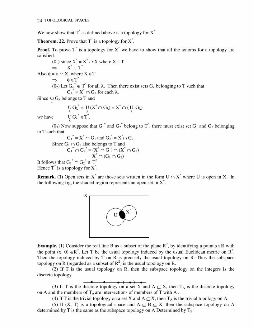
Remark. (1) Open sets in X* are those sets written in the form U ∩ X* where U is open in X. In the following fig, the shaded region represents an open set in X*. Example. (1) Consider the real line R as a subset of the plane R2, by identifying a point x∈R with the point (x, 0) ∈R2. Let T be the usual topology induced by the usual Euclidean metric on R2. Then the topology induced by T on R is precisely the usual topology on R. Thus the subspace topology on R (regarded as a subset of R2) is the usual topology on R. (2) If T is the usual topology on R, then the subspace topology on the integers is the discrete topology (3) If T is the discrete topology on a set X and A ⊆ X, then TA is the discrete topology on A and the members of TA are intersections of members of T with A . (4) If T is the trivial topology on a set X and A ⊆ X, then TA is the trivial topology on A. (5) If (X, T) is a topological space and A ⊆ B ⊆ X, then the subspace topology on A determined by T is the same as the subspace topology on A Determined by TB

U X*

TOPOLOGY 25

Theorem. 23. Let (X, T) be a topological space and A be a subset of X. Let B be a basis for T. Then BA = B ∩ A ; B ∈ B is a basis for the subspace topology on A.

Proof. Let U ∈ T and let x ∈ U. Then since B is a base for T, by definition, there is a member B ∈ I such that x∈B and B ⊆ U. Therefore x∈ B ∩ A ⊆ U ∩ A. Hence by the result “let (X, T) be a topological space and suppose B is a subcollection of T such that for each x∈X and each member U of T such that x∈∪, There is an element B of B such that x∈B and B ⊆ U. Then B is a basis for T.” We get, BA is the basis for the subspace topology on A.

Theorem. 24. Let (X, T) be a topological space and A be an open subset of X and TA is the induced or relative topology on A determined by T. If U ∈TA, then U ∈T.

Proof. Let U∈TA, then there is an open subset V of X such that U = A ∩ V. Since A and V are open in X, so is A ∩ V = U. Hence U ∈ T.

Continuous Functions

Definition. A function f mapping a topological space (X, T) into a topological space (X*, T*) is said to be continuous at a point x ∈ X if and only if for every open set G* containing f(x), there is an open set G containing x such that f(G) ⊆ G*

We say that f is continuous on a set E ⊆ X if and only if it is continuous at each point of E. Example. (1) Let X = 1, 2, 3, 4 and T = φ, (1), (2), (1, 2), (2, 3, 4), X. Define a mapping f : X→X by f(1) = 2, f(2) = 4, f(3) = 2 and f(4) = 3. Show that (1) f is not continuous at 3 and f is continuous at 4 . Analysis. The open sets containing f(3) = 2 are (2), (1, 2), (2, 3, 4) and X. We see that f−1(2) = (1, 3), f−1(1, 2) = (1, 3), f−1 (2, 3, 4) = (1, 3, 4, 2) and f−1(X) = (1, 2, 3, 4) = X itself. But we see that (1, 3) is not open as it does not belong to T. Hence f is not continuous at 3

Now we check continuity at the point 4. The open sets containing f (4) = 3 are the sets (2, 3, 4) and X. Now f−1 (2, 3, 4) = (1, 3, 4, 2) = X and f−1(X) = (1, 2, 3, 4) = X is open. Hence f is continuous at 4. (2) Let (X, T) be a discrete topological space and (Y, U) be any topological space. Then every function f : X→Y is necessarily continuous on X. For f−1(G), where G is open in Y is a subset of X and so open. (3) Let X = (x, y, z) and T = φ, (x), (y), (x, y), X so that (X, T) is a topological space. Define f : X→X by f(x) = x, f(y) = z and f(z) = y. Then by considering inverse images of the sets of T, we find that f is not continuous at x. (4) Let T denote the usual topology on R and define T : (R, T) → (R, T) by f(x) = x3 . The collection B of all open intervals is a basis for T. Let (a, b) be an open interval. Then f−1(a, b) = ( 33 b,a ) is open so inverse image of every open set is open (equivalent condition for continuity of f, proved below). Hence f is continuous.

TOPOLOGICAL SPACES

26

(5) Let (X, T) be a topological space and a singleton a be T-open. Suppose that (Y, T*) is another topological space. Then the function f : X→Y is continuous at a∈X.

Remark. Composition of two continuous mappings is continuous. Let the functions f and g be defined as follows If f : (X, T) → (Y, T*) and g : (Y, T*) → (Z, T**) If f and g are continuous, then gof is also continuous. We note that if G** is open in Z, then (gof)−1 [G**] = (f−1og−1) (G**) = f−1 [g−1(G**)] Since g is continuous, g−1 (G**) is open in Y, and then since f is continuous, f−1 [g−1(G**)] is open in X. Therefore gof is continuous on X.

Theorem. 25. Let (X, T) and (X*, T*) be topological spaces and f : X → X*, then the following conditions are each equivalent to the continuity of f on X. (1) The inverse image of every open set in X* is an open set in X. (2) The inverse image of every closed set in X* is a closed set in X. (3) f (C(E)) ⊆ C*(f(E)) for every E ⊆ X.

Proof. (1) Suppose that f is continuous on X and G* is an open set in X*. If x is any point of f−1(G*), and f is continuous at x, so there must exist an open set G containing x such that f(G) ⊆ G*. Thus G ⊆ f−1(G*) and hence f−1(G*) is an open set in X.

Conversely if the inverse images of open sets are open, we may choose the set f−1(G*) as the open set G required in the above definition. (2) Suppose that f is continuous and G* is closed in X*. Then f −1(X* − G*) = X − f −1(G*) Since f is continuous and X*− G* is open, it follows that X − f−1(G*) is open. Consequently f−1(G*) is closed.

Conversely let G** be an open subset of X*, then f −1[X* − G**] = X − f −1 (G**]

Since the left hand side is closed, it follows that X − f−1(G**) is closed which implies that f−1(G**) is open. Hence f is continuous. (3) Suppose that f is continuous on X and E is a subset of X. Since E ⊆ f−1 [f(E)] for any function, E ⊆ f −1[C*(f(E))]

But C*(f(E)) is closed and therefore f −1[C*(f(E))] is closed. Moreover this contains E. Therefore, C(E) ⊆ f −1 [C*(f(E))] and so f(C(E)) ⊆ f[f −1(C*(f(E))] ⊆ C*[f(E)] conversely suppose that f [C(E)] ⊆ C*[f(E)] (1) for all subsets E ⊆ X. let F* be a closed set in X*. Choose E = f−1(F*), we obtain f(C(E)] = f[C(f −1(F*))] ⊆ C* [f(f −1(F*))] [by (1)] ⊆ C*(F*) = F* since F* is closed. C(E) ⊆ f −1(F*) C[f −1(F*) ⊆ f −1(F*)

TOPOLOGY 27

f −1(F*) is a closed set. and so the inverse image of every closed set is a closed set.

Theorem. 26. Let [Tλ ; λ ∈ ∧] be an arbitrary collection of topologies on X and let (Y, V) be a topological space. If the mapping f : X→Y is Tλ−V continuous for all λ∈∧, then f is continuous with respect to the intersection topology T = ∩Tλ ; λ∈∧

Proof. Let G be an open set in Y. Since f is Tλ−V continuous, therefore f −1 (G) is open in X that is f −1(G) ∈Tλ for all λ∈∧ f −1(G) ∈ ∩Tλ ; λ ∈∧ f −1(G) ∈T. f is continuous with respect to T. Theorem. 27. If f is a continuous mapping of (X, T) into (X*, T*), then f maps every connected subset of X onto a connected subset of X*.

Proof. Let E be a connected subset of X and suppose that E* = f(E) is not connected. Then there must exist some separation E* = A*/B* where A* and B* are non-empty, disjoint, open subsets of E*. Then f being continuous, both f−1(A*) and f−1(B*) are open in X. Clearly A = f−1(A*) ∩ E and B = f−1 (B*) ∩ E are non-empty disjoint sets which are both open subsets of E. Thus E must have the separation E = A/B and so is not connected. Hence we get a contradiction. Thus E* is connected.

Remark. Any continuous image of a compact topological space is compact

Homemorphism

The first systematic treatment of continuity and homemorphism was given by Hausdorff.

Definition. Let X and Y be two topological spaces and f be a mapping from X into Y. Then f : X→Y is called an open mapping if and only if f(G) is open in Y whenever G is open in X.

Thus a mapping is open if and only if the image of every open set is an open set. Such mappings are also called interior mappings.

Similarly a mapping is closed if and only if image of every closed set is a closed set.

Remark. (1) Since there is no general containing relation between f(EC) and [f(E)]C. We find that an open (closed) mapping need not be closed (open), even if continuous. For example let (X, T) be any topological space and let (X*, T*) be the space for which X* = [a, b, c] and T* = [φ, a, a, c, X*. The transformation which takes each point of X into the point a is continuous open map which is not closed. The transformation which takes each point of X into b is a continuous closed map which is not open.

Remark. (2) As we know that continuity of a function does not really depend upon the topology on the entire co-domain but rather on the relative topology on the range. This is no longer true for openness of a function. Consider the function f : R→R2 defined by f(x) = (x, 0) for x∈R. Then f is not open with respect to the usual topologies on R and R2. The range of f is the x-axis of R2. If we regard f as a function from R to the x-axis (with relative topology), then it is open. Similarly, a restriction of an open function need not be open. These remarks also apply for closed functions.

Remark. (3) In order to show that a function is open, it is sufficient to show that it takes all members of a base for the domain space to open subsets of the co-domain. Using this fact, it it easy to show that projection functions from a product space to the co-ordinate spaces are open. It appears that they are also closed. But this is not the case. Consider the projection π1 : R2 →R,

TOPOLOGICAL SPACES

28

π1(x, y) = x (x, y∈R). Let H be the set (x, y) ∈ R2, xy = 1. Then H is a closed subset of R2 as its complement is open. However π1(H) is the set of all non-zero real numbers and it is not a closed subset of R.

Remark. (4) The following examples show that there is no direct relation between openness and continuity of a function. (i) Let T denote the discrete topology on R and let µ denote the usual topology on R. Then f : (R, T) → (R, µ) defined by f(x) = x for each x∈R is continuous because if U∈µ, then f−1(U) ∈T. However f is not open because 1∈T whereas 1 ∉ µ. (ii) The function g : (R, µ) → (R, T) defined by g(x) = x for all x∈R is open but not continuous.

Theorem 28. A mapping f of X into X* is open if and only if f[i (E)] ⊆ i*[f(E)] for every E ⊆ X.

Proof. Suppose f is open and E ⊆ X. Since i(E) is an open set and f is an open mapping, f(i(E)) is an open set in X*. Since i(E) ⊆ E, f(i(E)) ⊆ f(E). Thus f(i(E)) is an open set contained in f(E) and hence f(i(E)) ⊆ i*(f(E))

Conversely if G is an open set in X and f(i(E)) ⊆ i*(f(E)) for all E ⊆ X, then f(G) = f(i(G)) ⊆ i*(f(G)) and so f(G) is an open set in X*. Hence f is an open mapping.

Definition. Let X and Y be two topological spaces. Then a mapping f : X→Y is called a homemorphism if and only if it is bijective, continuous and open. Equivalently f : X→Y is a homemorphism if and only if it is bijective and bi-continuous. (By bi-continuous we mean that both f and f−1 are continuous)

Two topological spaces X and Y are said to be homeomorphic if there exists a homemorphism of X onto Y and in this case Y is called a homemorphic image of X.

A property of sets which is preserved by homemorphisms is called a topological property. The properties of a set being open, closed, connected, compact and dense in itself are topological properties but distances and angles are not the topological properties because they can be altered by suitable non-tearing deformations.

Remark. (1) If f : X→Y is a homemorphism, then X and Y are equivalent (as sets) since f is bijective. Also f and f−1 preserve open sets we may regard X and Y as equivalent topological spaces that is they may be thought of as indistinguishable from the topological point of view :

Remark. (2) Translations from f : R→R defined by f(x) = x + a are homemorphisms. Completeness of metric spaces is not a topological property i.e. a complete metric space can be homemorphic to an incomplete metric space.

Theorem. 29. Metrizabiliy is a topological property.

Proof. Let (X, d) be a metric space and (Y, V) be a topological space and suppose f : X→Y is a homemorphism. Define ρ : Y×Y → R by ρ((y1, y2)) = d(f−1(y1) f−1(y2)) We see that ρ is a metric on Y. Also the topology induced by ρ is T. Thus the property of metrizability is preserved under homemorphism.

Definition. A subset E of a topological space is called isolated if and only if no point of E is a limit point of E that is if E ∩ d(E) = φ.

TOPOLOGY 29

Theorem. 30. If f is a homemorphism of X onto X*, then f maps every isolated subset of X onto an isolated subset of X*.

Proof. Suppose E is an isolated subset of X and let x*∈ f(E), There must then exist a point x∈E such that f(x) = x*. Since E is isolated, x ∉ d(E) and so there must exist an open set G containing x such that E ∩ G − x = φ. But f is a homemorphism and so f(G) is an open set in X* which contain f(x) = x*. From the fact that f is one to one, it follows that f(E ∩ G − x) = f(E) ∩ f(G) −(x* = φ Thus x* ∉ d(f(E)) and so f(E) must be isolated.

Theorem. 31. Let (X, T) and (X*, T*) be two topological spaces. A one to one mapping f of X onto X* is homemorphism if f(C(E)) = C(f(E)) for every E ⊆ X.

Proof. Suppose first that f is a homemorphism and let E ⊆ X and G = f(E). Then f−1(G) = f−1(f(E)) = E. Since f is continuous f(C(E)) ⊂ C(f(E)) (1)

Moreover, since f−1 is continuous. f−1 [C(G)] ⊂ C[f−1(G)] f−1 (C(f(E))] ⊂ C[f−1(f(E))] f−1 [C(f(E))] ⊂ C(E) C(f(E)) ⊂ f(C(E)) (2)

From (1 and (2), we have f(C(E)) ⊂ C(f(E)) ⊂ f(C(E)) which proves the first part.

Conversely let us suppose that f(C(E)) = C(f(E)). We shall show that f is homemorphism. Since f is bijective, it is sufficient to show that f and f−1 are continuous. We are given that f(C(E)) = C(f(E)) f [C(E)] ⊆ C[f(E)] f is continuous. Also C[f(E)] ⊆ f[C(E)]

Let G = f(E). Then f−1(G) = f−1(f(E)) = E. Therefore, C[f(f−1(G))] ⊂ f[C(f−1(G))] f [f−1 (C(G))] ⊂ f [C(f−1(G))] f−1 [C(G)] ⊆ C(f−1 (G)] which proves that f−1 is continuous.

CONNECTEDNESS 30

2

CONNECTEDNESS

Connectedness was defined for bounded, closed subsets of Rn by Cantor in 1883, but this definition is not suitable for general topological spaces. In 1892, Camille Jordan (1838-1922) gave a different definition of connectedness for bounded closed subsets of Rn. Then in 1911, N. J. Lennes extended Jordan’s definition to abstract spaces Hausdorff’s Grundzuge der Mengenlehre was the first systematic study of connectedness.

Connectedness represents an extension of the idea that an interval is in one piece. Thus from the intuitive point of view, a connected space is a topological space which consists of a single piece. This property is perhaps to the simplest which a topological space may have and yet it is one of the most important applications of topology to analysis and geometry.

On the real line, for instance intervals are connected subspaces and as we shall see they are the only connected subspaces. Connectedness is also a basic notion in complex analysis, for the regions on which analytic functions are studied are generally taken to be connected open subspace of the complex plane.

In the portion of topology which deals with continuous curves and their properties, connectedness is of great significance, for whatever else a continuous curve may be, it is certainly a connected topological space.

Spaces which are not connected are also interesting. One of the outstanding characteristics of the cantor set is the extreme degree in which it fails to be connected. Much the same is true of the subspace of the real line which consists of rational numbers. These spaces are badly disconnected.

Our purpose in this chapter is to convert these rather vague notions into precise mathematical ideas and also to establish the fundamental facts in the theory of connectedness which rests upon them.

Connected Spaces Definition. A topological space is connected if it can not be expressed as the union of two non-empty disjoint open sets.

An equivalent formulation of this definition is that a set is said to be connected if and only if it has no separation.

Definition. Two subsets A and B form a separation or partition of a set E in a topological space (X, T) if and only if (i) E = A ∪ B (ii) A and B are non-empty (iii) A ∩ B = φ (iv) Neither A contains a limit point of B nor B contains a limit of A. If A and B form a separation of E, then we write E = A/B.

TOPOLOGY 31

Remark. The requirements that A and B are disjoint sets and neither contains a limit point of the other may be combined in the formula [A ∩ C(B)] ∪ [B ∩ C(A)] = φ which is often called the Hausdorff-Lennes separation condition and such subsets are called separated.

Thus a set is said to be connected if and only if whenever it is written as the union of two non-empty disjoint sets, at least one of them must contain a limit point of the other. We now give examples of some spaces that are connected.

Example (1) Empty set and every set consisting of one point is a connected set. Example (2) In the case of discrete topological space, only φ and the singleton are connected sets. Example (3) Let X be a non-empty set and T be the trivial topology on X. Then (X, T) is connected. Example (4) Every open interval is connected. Example (5) Let T be the usual topology on R. Then (R, T) is connected.

Analysis. The proof is by contradiction. Suppose (R, T) is not connected. Then there exist disjoint open sets U and V such that R = U ∪ V. Since U = R − V and V = R − U, U and V are also closed. Let a ∈ U and b ∈V. We may assume w. l. o. g. that a < b. Let W = U ∩ [a, b]. Since W is bounded, it has a least upper bound c. Since W is closed. c ∈ W. Since W ∩ V = φ, c ≠ b. Also c is the least upper bound of W, (c, b] ⊆ V. Therefore c ∈V, but V is closed so c ∈V. Therefore c ∈ U ∩ V. This is contradiction because U ∩ V = φ.

Theorem. 32. A topological space (X, T) is connected if and only if it can not be expressed as the union of two non-empty sets that are separated in X. Proof. Suppose X is not connected. Then there are non-empty, disjoint open sets U and V such that X = U ∪ V. Then U and V are closed so that U ∩ V = U ∩ V = φ and U ∩V = U ∩ V = φ. Therefore U and V are separated in X.

Suppose now that there are non-empty subsets A and B such that X = A ∪ B and A ∩ B = A ∩B = φ. Since X = A ∪ B and A ∩ B = φ A ⊆ A so that A is closed. Similarly B is closed. Therefore A and B are also open and hence X is not connected.

Remark. If A and B form a separation of the topological space (X, T), then A and B are both open and closed.

Theorem. 33. A topological space (X, T) is connected if and only if no non-empty proper subset of X is both open and closed.

Proof. Suppose X is not connected. Then there are non-empty disjoint open sets U and V such that X = U ∪ V. Thus U is a non-empty proper subset of X that is both open and closed.

Suppose X has a non-empty proper subset U that is both open and closed. Then U and X − U are non-empty disjoint open sets whose union is X. Therefore X is not connected.

The following result provides useful ways of formulating the definition of connectedness for subspaces of a topological space.

Theorem. 34. Let (X, T) be a topological space and let A ⊆ X. Then the following conditions are equivalent. (a) The subspace (A, TA) is connected.

CONNECTEDNESS 32

(b) The set A can not be expressed as the union of two non-empty sets that are separated in X. (c) There do not exist U, V ∈T such that U ∩ A ≠ φ, U ∩ V ∩ A = φ and A ⊆ U ∪ V. Proof. First we prove (a) b. In each case, we prove by contradiction. (a) (b). Suppose the subspace (A, TA) is connected and U and V are non-empty sets such that A = U ∪ V and U ∩ V = U ∩V = φ.

Then U and V are separated in A, so by Theorem. 32, A is not connected (b) (c). Suppose there exist U, V ∈T such that U ∩ A ≠ φ, V ∩ A ≠ φ, U ∩ V ∩ A = φ

and A ⊆ U ∪ V.

Then U ∩ A and V ∩ A are non-empty sets that are separated in X and A = (U ∩ A) U (V ∩ A) (c) (a). Suppose (A, TA) is not connected.

Then there exist U′, V′, ∈ TA such that U′ ≠ φ ≠ V′ and U′ ∩ V′ = φ and A = U′ ∪ V′. Thus there exist U, V∈T such that U′ = A ∩ U and V′ = A ∩ V.

It is clear that U ∩ A ≠ φ, V ∩ A ≠ φ, U ∩ V ∩ A = φ and A ⊆ U ∪ V.

Theorem. 35. A subspace of the real line R is connected if and only if it is an interval. In particular, R is connected.

Proof. Let X be a subspace of R. We first prove that if X is connected, then it is an interval. We do this by assuming that X is not an interval and by using this assumption to show that X is not connected. To say that X is not an interval is to say that there exist real numbers x, y, z such that x < y < z, x and z are in X, y is not in R. Thus X = X ∩ (−∞, y) UX ∩ (y, + ∞) is a disconnection of X, so X is disconnected.

Now we prove the second part. We show that if X is an interval, then it is necessarily connected. We first assume that X is disconnected. Let X = A ∪ B be a disconnection of X. Since A and B are non-empty, we can choose a point x in A and a point z in B. A and B are disjoint, so x ≠ z, w. l. o. g. we assume that x < z. Since X is an interval, [x, z] ⊆ X and each point in x, z is in either A or B. We now define y by y = sup ([x, z] ∩ A). It is clear that x ≤ y ≤ z, so y is in X. Since A is closed in X, the definition of y shows that y is in A. From this we conclude that y < z. Again by the definition of y, y + ∈ is in B for every ∈ > 0 such that y + ∈ ≤ z, and since B is closed in X, y is in B. We have proved that y is in both A and B, which contradicts our assumption that these sets are disjoint.

Theorem. 36. Any continuous image of connected space is connected.

Proof. Let f : X→Y be a continuous mapping of a connected space X into an arbitrary topological space Y. We must show that f(X) is connected as a subspace of Y. Assume that f(X) is disconnected. This means that there exist two open subsets G and H of Y whose union contains f(X) and whose intersections with f(X) are disjoint and non-empty. This implies that X = f −1(G) ∪ f −1(H) is a disconnection of X, which contradicts the connectedness of X.

Remark. Thus from the above theorem, it follows that property of connectedness is preserved by continuous mappings.

Theorem 37. If E is a subset of a subspace (X*, T*) of a topological space (X, T), then E is T* connected if and only if it is T-connected.

TOPOLOGY 33

Proof. In order to have a separation of E with respect to either topology, we must be able to write E as the union of two non-empty disjoint sets. If A and B are two non-empty disjoint sets, whose union is E, then A, B ⊆ X* ⊆ X Calculating with the Hausdorff – Lennes separation condition, we find that [A ∩ C*(B)] ∪ [C*(A) ∩ B] = [A ∩ X* ∩ C(B)] ∪ [X* ∩ C(A) ∩ B] = [A ∩ X* ∩ C(B)] ∪ [X* ∩ C(A) ∩ B] = [A ∩ C(B)] ∪ [B ∩ C(A)] Thus if the condition is satisfied with respect to one topology, then it is satisfied with respect to the other.

Remark. The above theorem leads us to say that connectedness is an absolute property of sets that it does not depend on the space in which the set is contained except that the topology, of course must be the relative topology.

Theorem. 38. If E is a connected subset of a topological space (X, T), which has a separation X = A/B, then either E ⊆ A or E ⊆ B.

Proof. Clearly E = E ∩ X = E ∩ (A ∪ B) = (E ∩ A) ∪ (E ∩ B)

Since X = A/B, we have [(E ∩ A) ∪ C(E ∩ B)] ∪ [C(E ∩ A) ∩ (E ∩ B)] ⊆ [A ∩ C(B)] ∪ [C(A) ∩ B] = φ since A and B are separations.

Thus if we assume that both E ∩ A and E ∩ B are non-empty, we have a separation for E = (E ∩ A)/(E ∩ B). Hence either E ∩ A is empty so that E ⊆ B, or E ∩ B is empty so that E ⊆ A.

Cor. 1. If C is a connected set and C ⊆ E ⊆ C(C), then E is a connected set.

Proof. Suppose that E is not a connected set, then it must have a separation E = A/B. By the above theorem, since C is a subset of E which has a separation, C must be contained in A or contained in B. Without loss of generality, let us suppose that C ⊆ A. From this it follows that C(C) ⊆ C(A) and hence C(C) ∩ B ⊆ C(A) ∩ B = φ. On the other hand, B ⊆ E ⊆ C(C) and so C(C) ∩ B = B, thus we must have B = φ, which contradicts our hypothesis that E = A/B. Hence E is connected.

Cor. 2. If every two points of a set E are contained in some connected subset C of E, then E is a connected set.

Proof. If E is not connected, then it must have a separation E = A/B. Since A and B must be non-empty, let us choose points a∈A and b∈B. From the hypothesis we know that a and b must be contained in some connected subset C contained in E. Then by the above theorem, either C ⊆ A or C ⊆ B. Since A and B are disjoint, this is a contradiction to the fact that C contains points of A as well as of B. Hence E is connected.

Cor. 3. The union E of any family Cλ of connected sets having a non-empty intersection is a connected set

CONNECTEDNESS 34

Proof. Suppose E is not connected, then it must have a separation E = A/B, By hypothesis, we may choose a point x∈

∩ Cλ which implies that x∈Cλ for each λ. The point x must belong to

either A or B and w.l.o.g. let us suppose x∈A. Then since x∈Cλ for each λ, we have Cλ ∩ A ≠ φ for every λ. Now by the above theorem, each Cλ must be either a subset of A or a subset of B. Since A and B are disjoint and Cλ ∩ A ≠ φ. We must have Cλ ⊆ A for all λ. And so E =

∪ Cλ ⊆

A. From this we obtain the contradiction that B = φ. Hence E is connected.

Cor. 4. If A and B are connected sets, then A ∪ B is connected.

Proof. Suppose A ∪ B is not connected, then it must have a separation A ∪ B = C/D.

Since A is a connected subset of A ∪ B, either A ⊆ C or A ⊆ D. Similarly we have either B ⊆ C or B ⊆ D. Now if A ⊆ C, A ∪ B ⊆ C, A ∪ B ⊆ D. But C and D are disjoint. Hence contradiction. Thus A ∪ B is connected.

Theorem. 39. If a connected set C has a non-empty intersection with both a set E and the complement of E in a topological space (X, T), then C has a non-empty intersection with the boundary of E.

Proof. We will show that if we assume that C is disjoint from b(E), we obtain the contradiction that C is not connected i.e. C = (C ∩ E)/(C ∩ EC). From C = C ∩ X = C ∩ (E ∪ EC) = (C ∩ E) ∪ (C ∩ EC) we see that C is the union of two sets. These two sets are non-empty by hypothesis.

If we calculate (C ∩ E) ∩ C(C ∩ EC) ⊆ [ C ∩ C(E)] ∩ C(EC) = C ∩ [C(E) ∩ C(EC)] = C ∩ b(E) we see that the assumption that C ∩ b(E) = φ leads to the conclusion that (C ∩ E) ∩ (C ∩ EC) = φ. In the same way, we may show that C[C ∩ E] ∩ [C ∩ EC] = φ and we have a separation of C.

Theorem. 40. A topological space X is disconnected if and only if there exists a continuous mapping of X onto the discrete two point space 0, 1.

Proof. If X is disconnected and X = A ∪ B is a disconnection, then we define a continuous mapping f of X onto 0, 1 by the requirement that f(x) = 0 if x ∈ A and f(x) = 1 if x ∈B. This is valid since A and B are disjoint and their union is X. Also A and B are non-empty and open, f is clearly onto and continuous.

On the other hand, if there exists such a mapping, then X is disconnected for if X were connected, then by the result that a continuous image of a connected space is connected, 0, 1 is connected but we know that a subspace of the real line R is connected if and if it is an interval. Thus X is connected would lead to a contradiction. Hence X is disconnected.

Theorem. 41. The product of any non-empty class of connected spaces is connected.

TOPOLOGY 35

Proof. Let Xi be a non-empty class of connected spaces and form their product X = ∏i

iX . We

assume that X is disconnected and we deduce a contradiction from this assumption. Now by the above theorem there exists a continuous mapping f of X onto the discrete two point space 0, 1. Let a = ai be a fixed point in X and consider a particular index i1. We define a mapping

1i1iXoff into X by means of )x(

1i1if = yi), where yi = ai for i ≠ i1 and

1i1ixy = . This is clearly

a continuous mapping, so 1i

ff is a continuous mapping of 1i

X into 0, 1. Since 1i

X is connected,

1iff is constant and

(1i

ff ) (1i

X ) = f(a)

for every point 1i1i

Xinx . This shows that f(x) = f(a) for all x′s in X which equal a in all co-

ordinate spaces except 1i

X . By repeating this process with another index, i2, etc, we see that

f(x) = f(a) for all x′s in X. which equal a in all but a finite number of co-ordinate space. The set of all x′s of this kind is a dense subset of X, and so f is a constant mapping this contradicts the assumption that f maps X onto 0, 1 and this completes the proof.

Components

Definition. Let (X, T) be a topological space and x be a point of a subset E contained in X, then union of all connected sets containing x and contained in E, is called the component of E corresponding to x and will be denoted by C (E, x). Since union of connected sets is connected, C(E, x) is a connected set. Hence C(E, x) is the largest connected subset of E containing x. Thus a connected space clearly has only one component, namely the space itself.

Components corresponding to different points of E are either equal or disjoint, so that we may speak of the components of a set E without any reference to specific points. Every subset of a topological space has now been partitioned with disjoint subsets, its components.

Example. (1) Let (X, T) be a discrete space and x∈X be arbitrary. Then x is a connected subset of X and also x is not a proper subset of any connected subset of X. Hence by definition, x is a component of X. Thus each point of a discrete space (X, T) is a component of X. (2) If X is connected, then X has only one component, X itself. (3) Every indiscrete space has only one component, namely the space itself. (4) Let X = a, b, c, d, e consider the following topology on X. T = X, φ, a, c, d, a, c, d, b, c, d, e

The components of X are a and b, c, d, e. Any other connected subset of X, such as b, d, e is a subset of the one of the components.

Theorem. 42. The components of a topological space (X, T) are closed subsets of X.

Proof. Let C be the component of X. Since C is connected, its closure C(C) is also connected. Let a be a point of C and b be a point of C(C). Then the connected set C(C) contains both a and b. But by definition, C is the largest connected set containing a and so b∈C. Hence C(C) ⊆ C and thus C is closed.

Theorem. 43. Let X be an arbitrary topological space, then we have the following (1) Each point in X is contained in exactly one component of X. (2) Each connected subspace of X is contained in a component of X. (3) A connected subspace of X which is both open and closed is a component of X.

CONNECTEDNESS 36

Proof. (1) Let x be a point in X. Consider the class Ci of all connected subspaces of X which contain x. This class is non-empty, since x itself is connected. Since union of connected sets having a non-empty intersection is connected, C = Ui Ci is a connected subspace of X which contains x. C is clearly maximal and therefore a component of X, because any connected, subspace of X which contains C is one of the Ci’s and is thus contained in C. Finally, C is the only component of X which contains x. For if C*, is another, it is clearly among the Ci’s, and is therefore contained in C and since C* is maximal as a connected subspace of X, we must have C* = C. (2) This is a direct consequence of the construction above and from this it follows that, a connected subspace of X is contained in the component which contains any one of its points. (3) To prove (3), let A be a connected subspace of X which is both open and closed. By (2) above, A is contained in some component C. If A is a proper subset of C, then C = (C ∩ A) ∪ (C ∩ A′) is a disconnection of C. This contradicts the fact that C, being a component is connected and we conclude that A = C. Thus a connected subspace of X which is both open and closed is a component of X.

Locally Connected Definition. A topological space (X, T) is said to be locally connected if and only if for every point x∈X and every open set G containing x, there exists a connected open set G* containing x and contained in G

Thus a space is locally connected if and only if the family of all open connected sets is a base for the topology for the space. We know that local compactness is implied by compactness local connectedness, however neither implies, nor is implied by connected as shown below.

Remark. (1) A locally connected set need not be connected. For example, a set consisting of two disjoint open intervals is locally connected but not connected (2) A connected subset of the plane which is not locally connected. For each positive integer n, let us denote by En, the line segment connecting the origin to the point

< 1, n1

>. Each of these line segments is connected and all contain the origin, so their union is

connected (since the intersection is the origin being a common point). If we let X be the point <1,

0> and Y be the point <21

, 0>, then X and Y are both limit points of the set consisting of all the

En’s

Then E = X ∪ Y ∪ (Un En is a connected set. This set is not locally connected, however since an open set containing X if sufficiently small will not contain a connected open set containing X.

Example. (1) Let (X, D) be a discrete topological space. We know that for every x∈X, the singleton x is connected and is such that x contains x and is contained in an open connected set x. Hence a discrete topological space is locally connected. (2) Every Banach space is locally connected (3) The union of two disjoint open intervals on the real line is a simple example of a space which is locally connected but not connected.

Remark. Removal of a point from a connected set leaves a set which is not connected.

TOPOLOGY 37

Theorem. 44. A space X is locally connected if and only if for every open set U of X, each component of U is open in X.

Proof. Suppose that X is locally connected and let U be an open set in X and further let C be a component of U. If x is a point of C, we can choose a connected open neighbourhood V of x such that V ⊂ U. Since V is connected, it must be entirely in the component C of U. Therefore C is open in X.

Conversely, suppose that components of open sets in X are open. Given a point x of X and a neighbourhood U of x, let C be the component of U containing x. Since C is a connected subset of U. Thus for every open set U containing x, there is a connected open set C containing x such that C ⊂ U. Hence X is locally connected.

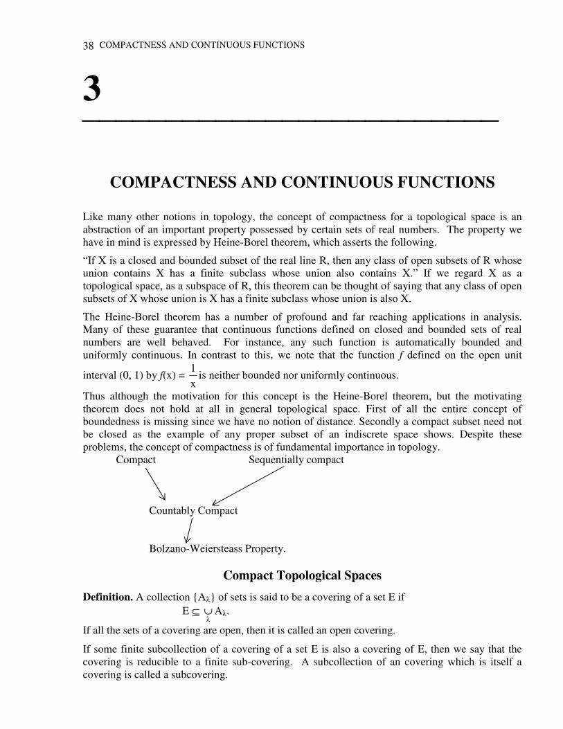
COMPACTNESS AND CONTINUOUS FUNCTIONS 38

3

COMPACTNESS AND CONTINUOUS FUNCTIONS

Like many other notions in topology, the concept of compactness for a topological space is an abstraction of an important property possessed by certain sets of real numbers. The property we have in mind is expressed by Heine-Borel theorem, which asserts the following.

“If X is a closed and bounded subset of the real line R, then any class of open subsets of R whose union contains X has a finite subclass whose union also contains X.” If we regard X as a topological space, as a subspace of R, this theorem can be thought of saying that any class of open subsets of X whose union is X has a finite subclass whose union is also X.

The Heine-Borel theorem has a number of profound and far reaching applications in analysis. Many of these guarantee that continuous functions defined on closed and bounded sets of real numbers are well behaved. For instance, any such function is automatically bounded and uniformly continuous. In contrast to this, we note that the function f defined on the open unit

interval (0, 1) by f(x) = x1

is neither bounded nor uniformly continuous.

Thus although the motivation for this concept is the Heine-Borel theorem, but the motivating theorem does not hold at all in general topological space. First of all the entire concept of boundedness is missing since we have no notion of distance. Secondly a compact subset need not be closed as the example of any proper subset of an indiscrete space shows. Despite these problems, the concept of compactness is of fundamental importance in topology.

Compact Sequentially compact Countably Compact Bolzano-Weiersteass Property.

Compact Topological Spaces

Definition. A collection Aλ of sets is said to be a covering of a set E if E ⊆

∪ Aλ.

If all the sets of a covering are open, then it is called an open covering.

If some finite subcollection of a covering of a set E is also a covering of E, then we say that the covering is reducible to a finite sub-covering. A subcollection of an covering which is itself a covering is called a subcovering.

TOPOLOGY 39

Definition. Let (X, T) be a topological space. A collection Gi of open subsets of X is said to be an open covering of X if X =

i∪ Gi

A subset E of a topological space (X, T) is said to be compact if and only if every open covering of E is reducible to a finite subcovering of E i.e. every open covering of E has a finite subcovering.

Example. (1) If X is a finite set and T is a topology on X, then (X, T) is compact. (2) If T is the finite complement topology on any set X, then (X, T) is compact. Now we give some examples of spaces which are not compact.

(1) If X is an infinite set and T is the discrete topology on X, then (X, T) is not compact.

(2) The open interval (0, 1) is not compact because

∈

Nn;1,n1

is an open cover that

does not have a finite sub-cover. (3) The real line is not compact because (−n, n); n∈Nis an open cover that does not have

a finite subcover. (4) The real line with the lower limit topology is not compact since [n, n+1) ; n ∈ Z is an

open cover that does not have a finite subcover.

Definition. A topological property is said to be weakly hereditary if whenever a space has it, so does every closed subspace of it.

Theorem. 1. If E is a subset of a subspace (X*, T*) of a topological space (X, T), then E is T* compact if and only if it is T-compact.

Proof. Suppose E is T*-compact and Gλ is some T-open covering of E. We shall show that Gλ has a finite subcovering. The family of sets X* ∩ Gλ clearly forms a T*−open covering of E since E = X* ∩ E = X*∩ (

∪ Gλ)

=

∪ (X* ∩ Gλ)

Since E is T*−compact, there is a finite subcovering of E such that

E ⊆ n

1i=∪ [X* ∩ Gi] ⊆

n

1i=∪ Gi

Thus we have shown that every open covering of E has a finite subcovering and hence E is T-compact.

Conversely suppose that E is T-compact and G*λ is some T*−open covering of E. From the

definition of induced topology, each Gλ* = X* ∩ Gλ for some T−open set Gλ.

The family Gλ is clearly a T−open covering of E and so there must be some finite subcover of E

such that E ⊆ n

1i=∪ Gi

But then we have, E = X* ∩ E

⊆ X* ∩ (n

1i=∪ Gi)

=n

1i=∪ (X* ∩ Gi) =

n

1i=∪ Gi

*

which is a finite subcovering of E from Gλ*

Hence E is T*−compact.

COMPACTNESS AND CONTINUOUS FUNCTIONS 40

Remark. The property of compactness is not Heriditary. It is weakly Heriditary. We do however the following result.

Theorem 2. Every closed subset of a compact space is compact.

Proof. Let G be an open covering of a closed subset E of a compact space (X, T), then G* = G ∪ EC

is an open covering of X. Since (X, T) is compact, every open covering of X has a finite subcovering. If we remove EC from the finite subcovering of X, we will have a finite subcovering of E chosen from G. Hence E is compact.

Example. The cantor set C is the intersection of closed subsets of R. Therefore C is closed subset of R and hence of I = [0, 1]. Since I is compact by the above theorem, thus C is compact being the closed subset of a compact space.

Remark. The following example shows that a compact subset of a topological space is not necessarily closed.

For example let T be the finite complement topology on R and let A = x ∈R, x is rational Then A is compact but not closed.

But if the space is Hausdorff, then every compact subset is closed.

First of all we give some definitions.

Definition. A topological space (X, T) is a T1−space provided that for each pair x, y of distinct points of X, there exist open sets U and V such that x ∈U, y ∉U, y ∈V and x ∉V.

Definition. A topological space (X, T) is a Hausdorff space provided that if x and y are distinct members of X then there exist disjoint open sets U and V such that x∈U and y∈V.

Theorem. 3. Let (X, T) be a Hausdorff space, let A be a compact subset of X and p Î X - A. Then there exist disjoint open sets U and V such that A ⊆ U and p∈V.

Proof. Since X is Hausdorff and A is a subset of X, for each x∈A, there are disjoint open sets Ux and Vx such that x∈Ux and p∈Vx. Then µ = Ux ; x∈A is an open cover of A. Since A is compact subset of X, there is a finite subcollection

nx2x1x U,...,U,U of µ that cover A. For each i

= 1, 2,…,n, ixU and the corresponding

ixV are disjoint. Therefore U = n

1i=∪

ixU and V =n

1i=∩

ixV are

disjoint open sets such that A ⊆ U and p∈V.

Cor.1. Every compact subset of a Hausdorff space is closed.

Proof. Let A be a compact subset of a Hausdorff space (X, T) and let p ∈ X −A. Then by Theorem 3, there is a neighbourhood U of p such that U ⊆ X −A. Therefore X−A is open and so A is closed. Hence every compact subset of Hausdorff space is closed.

Thus we have proved that a subset A of a compact Hausdorff space is compact if and only if it is closed.

Theorem. 4. Any continuous image of a compact set is compact.

Proof. Let f : X→Y be a continuous mapping of a compact set X into an arbitrary topological space Y mapping a compact set E into f(E). We must show that f(E) is compact in Y.

Suppose that Gλ* is an open covering of f(E).

Since E ⊆ f−1 (f(E))

TOPOLOGY 41

⊆ f−1

[∪ Gλ*]

⊆

[∪ f−1 [Gλ*]

Since f−1 (Gλ*) is open in X. It follows that f−1(Gλ

*) is an open covering of E. Since E is compact, there must be some finite subcovering of E i.e.

E ⊆ n

1i=∪ f−1(Gλ

*)

But then f(E) ⊆ f(n

1i=∪ f−1(Gi

*))

= n

1i=∪ f(f−1(Gi

*))

⊆ n

1i=∪ Gi

*

and so we have a finite subcover for f(E). Hence f(E) is compact. Theorem 5. A topological space is compact if and only if every class of closed sets with empty intersection has a finite subclass with empty intersection.

Proof. First assume that topological space (X, T) is compact, then a class of open sets is an open covering X = ∪Gi XC = ∩ Gi

C ∩ Gi

C = φ Since Gi’s are open Gi

C’s are closed. Thus the class of closed sets has empty intersection. Since this open covering is reducible to a finite subcovering

X = n

1i=∪ Gi XC = (

n

1i=∪ Gi)C

φ = n

1i=∩ Gi

Thus every class of closed sets with empty intersection has a finite subclass with empty intersection. Similarly the other part follows.

Theorem. 6. Let (X, T) be a topological space and let B be a basis for T. Then (X, T) is compact if and only if every cover of X by members of B has a finite subcover.

Proof. Let (X, T) be a compact space and let µ be a cover of X by members of B. Then µ is an open cover of X and hence it has a finite subcover since X is compact.

On the other hand suppose every open cover of X by members of B has a finite subcover. We shall show that X is compact. Let µ be an open cover of X. For each ∪∈µ, there is a subcollection B∗ of B such that U = ∪B ; B ∈ B∗. Since every member of U is union of members of subcollection of B∗ B.

Now, B ; B∈B∗ for some ∪ ∈ µ is an open cover of X by members of B and hence it has a finite subcover µ*. For each B∈µ*, choose a member UB of µ such that B ⊆ UB. Then UB ; B∈µ* is a finite subcollection of µ that covers X. Hence X is compact.

Theorem. 7. Every continuous real valued function on a compact space is bounded and attains its extrema.

COMPACTNESS AND CONTINUOUS FUNCTIONS 42

Proof. Let X be a compact space and suppose f : X→R is continuous. First we show f is bounded. For each x∈X, let Jx be the open interval (f(x)−1, f(x) +1) and let Vx = f−1(Jx).

By continuity of f, Vx is an open set containing x. Note that f is bounded on each Vx. Now the family Vx ; x∈X is an open cover of X and by compactness of X, admits a finite subcover say

nx2x1x V...,,V,V .

Let M = max f(x1), f(x2),…, f(xn) + 1 and let m = min f(x1), f(x2),…, f(xn) − 1

Now for any x∈X, there is some i such that x∈ ixV . Then f(xi) −1 < f(x) < f(xi) + 1 and so

m < f(x) < M showing that f is bounded. It remains to show that f attains its bounds.

Let L, M be respectively the supremum and infimum of f over X. If there is no point x in X for

which f(x) = L, then we define a new function g : X→R by g(x) = )x(L

1f−

for all x∈X. Then g

is continuous since f is so. However g is unbounded, for given any R > 0, there exists x such that

f(x) > L −R1

and hence g(x) > R. But this contradicts the above part of the theorem and hence f

attains the value L. Similarly f attains the infimum M.

Theorem. 8. Let (X, T) be a compact locally connected space. Then (X, T) has a finite number of components.

Proof. Suppose (X, T) has infinite number of components. Then since each component of X is open. Thus the collection of components of X is an open cover of X that does not have a finite subcover. Since X is compact, this is a contradiction. Hence a compact locally connected space has a finite number of components.

Remark. The following is the classical theorem of Heine-Borel Lebesgue.

Theorem. 9. A subset of the Euclidean n-space is En compact if and only if it is closed and bounded.

Proof. Let A be a compact subset of En. Since En is Hausdorff and A is a compact subset of Hausdorff space En, A is closed. Because of compactness. A can be covered by a finite family of open spheres of radius one and because each of these is bounded, A is bounded. Thus every compact subset of En is closed and bounded.

To prove the converse suppose that A is closed and bounded subset of En. Let Bi be the image of A under the projection into the ith co-ordinate space and note that each Bi is bounded because the projection decreases distances.

Then A ⊂ Π Bi, i = 0, 1,…, n−1 and this set is a subset of a product of closed bounded intervals of real numbers. Since A is a closed subset of the product and the product of compact spaces is compact, the proof reduces to showing that a closed interval [a, b] is compact relative to the usual topology. Let µ be an open cover of [a, b] and let C be the supremum of all members x of [a, b] such that some finite subfamily of µ covers [a, x]. Choose U in µ such that C∈U and choose a member d of the open interval (a, c) such that [d, c] ⊂ U. There is a finite subfamily of µ which covers [a, b] and this family with U adjoined covers [a, c] . Unless c = b the same finite subfamily covers [a,d] an interval to the right of c, which contradicts the choice of c . Hence the result.

TOPOLOGY 43

Finite Intersection Property Definition. A family of sets will be said to have the finite intersection property if and only if every finite subfamily of the family has a non-empty intersection.

Theorem. 10. A topological space (X, T) is compact if and only if any family of closed sets having the finite intersection property has a non-empty intersection.

Proof. Suppose that (X, T) is compact and Fλ is a family of closed sets whose intersection is empty that is

∩ Fλ = φ

(

∩ Fλ)C = φC = X

X =

∪ FλC

and therefore,

∪ FλC is a covering of X, but (X, T) is given to be compact, therefore there exists

finite subcovering of X i.e.

X = n

1i=∪ Fi

But then φ = XC = (n

1i=∪ Fi

C)C = n

1i=∩ Fi

so that the family Fλ can not have the finite intersection property. Thus we arrive at a contradiction. Hence

∩ Fλ ≠ φ

Conversely suppose that (X, T) is not compact. This means that there exists an open covering Gλ of X which has no finite subcovering. To say that there is no finite subcovering means that complement of the union of any finite number of members of the cover is non-empty,

i.e. C

n

1

)G(=

∪ ≠ φ

C

n

1

G=

∩ ≠ φ by De-Morgan’s Law thus GλC is then a family of closed sets with

finite intersection property. Since Gλ is a covering of X, we have φ = XC = (

∪ Gλ)C =

∩ GλC

Thus this family of closed sets with the finite intersection property has an empty intersection which contradicts our hypothesis. Hence (X, T) is compact.

Countably Compact and Sequentially Compact Definition. A topological space (X, T) has the Bolzano-Weieistrrass property provided that every infinite subset of X has a limit point.

Definition. A topological space (X, T) is countably compact provided every countable open cover of X has a finite subcover.

Theorem. 11. A topological space (X, T) is countably compact if and only if every countable family of closed subsets of X with the finite intersection property has a non-empty intersection.

Proof. Suppose (X, T) is countably compact. Let A = Aα; α ∈∧ b a countable family of closed subsets of X with the finite intersection property. Suppose

∧∈∩

Aα = φ. Let

COMPACTNESS AND CONTINUOUS FUNCTIONS 44

µ = X −Aα ; α∈∧ Since

∧∈∪

(X − Aα) = X−∧∈

∩

Aα = X − φ = X.

If µ is an open cover of X. Since X is countably compact, there exists a finite number α1, α2,…, αn of members of ∧ such that X − Aα ; i = 1, 2,…, n covers X.

Thus X = n

1i=∪ (X−Aα) = X −

n

1i=∩ Aα and hence

n

1i=∩ Aα = φ. This is a contradiction.

Hence ∧∈

∩

Aα ≠ φ.

Suppose every countable family of closed subsets of X with the finite intersection property has a non-empty intersection. Let µ = Uα ; α ∈∧ be a countable open cover of X.

Suppose µ does not have a finite subcover.

Let A = X − Uα ; α ∈∧. Then A is a countable family of closed subsets of X. Let T be a finite subset of ∧. Since µ does not have a finite subcover,

∈∩ (X −Uα) = X −

∈∪ Uα ≠ φ.

Therefore A has the finite intersection property.

Hence ∧∈

∩

(X−Uα) ≠ φ since we have assumed that every countable family of closed subsets of X

with the finite intersection property has a non-empty intersection. But this is contradiction since

∧∈∩

(X−Uα) = X −∧∈

∪

Uα = X − X = φ

Therefore (X, T) is countably compact.

Theorem. 12. Every countably compact topological space has the Bolzano-Weierstrass property.

Proof. Let (X, T) be a countably compact space and A be an infinite subset of X. Since A is infinite. A contains a countably infinite set B = xi, i∈N. We may assume that if i ≠ j, then xi ≠ xj. The proof is by contradiction.

Suppose B has no limit point. Then for each n ∈N, Cn = xi∈B ; i ≥ n is a closed set.

Further, Cn ; n ∈N has the finite intersection property. Therefore by the result “A topological space (X, T) is countably compact if and only if every countable family of closed subsets of X

with the finite intersection property has a non-empty intersection”, ∞

=∩

1nCn ≠ φ. But if xK∈B, then

xK∉ CK+1, and hence

x ∉∞

=∩

1n Cn. Therefore

∞

=∩

1nCn = φ

and we have a contradiction. Thus B has a limit point and B ⊆ A, A has a limit point, thus every infinite subset of X has a limit point and hence (X, T) has the Bolzano-Wierstrass property.

Remark. The converse of the above theorem is not true in a general topological space. It holds for T1 space.

TOPOLOGY 45

Definition. A topological space (X, T) is a T1−space provided that for each pair x, y of distinct points of X, there exist open sets U and V such that x∈U, y ∉U and y∈V, x∉V.

Theorem. 13. Let (X, T) be a T1−space. Then X is countably compact if and only if it has the Bolzano-Weiersttrass property.

Proof. Suppose (X, T) has the Bolzano-Weierstrass property. The proof that X is countably compact is by contradiction. Suppose Un ; n ∈N is a countable open cover of X that has no finite subcover. Then for each n∈N,

Cn = X − n

1i=∪ Ui is a non-empty closed set.

For each n∈N, let pn∈Cn and let A = pn ; n∈N If A is finite, there exists p∈A such that pn = p for an infinite number of n∈N. Thus for each n∈N, p∈Cn.

This is a contradiction since Un ; n ∈N covers X. Suppose that A is infinite. Then by hypothesis, there is a point p∈X that is a limit point of A.

Since X is a T1−space and p is a limit point of A, then every neighbourhood of p contains an infinite number of members of A. Therefore for each n∈N, p is a limit point of An = pi ∈A; i > n. For each n∈N, An ⊆ Cn. Since for each n∈N, Cn is closed, p∈Cn. Once again this is a contradiction, since Un ; n∈N covers X. Therefore X is countably compact. The other part is already proved in the above theorem.

Theorem. 14. A compact topological space is countably compact.

Proof. We assume that the topological space X is compact and show that every infinite subset of X has a limit point in X i.e. it is countably compact.

Let E be an infinite subset of X with no limit point in X. So there must exist an open set Gx containing x such that E ∩ Gx − x = φ Clearly E ∩ Gx contains at the most one point x itself. Since the family Gxx∈X forms an open covering of the compact space X, therefore there must be some finite subcovering i.e.

X = n

1i=∪ Gxi

From this, it follows that

E = E ∩ X = E ∩ (n

1i=∪ Gxi)

= n

1i=∪ (E ∩ Gxi)

Since E ∩ Gxi contains at the most one point, Therefore E being the finite union of such sets contains at most n elements and so is finite. This leads to the contradiction. Hence every infinite subset of X must have at least one limit point.

Definition. A topological space (X, T) is sequentially compact provided every sequence in X has a subsequence that converges.

There is no direct relationship between compactness and sequential compactness. We give two examples.

COMPACTNESS AND CONTINUOUS FUNCTIONS 46

Example of a compact space that is not sequentially compact

For each α∈R, let Xα = I and X = R

∈

Xα. Then (X, T) is compact but not sequentially compact.

Example of a sequentially compact space that is not compact. Let (Ω, ≤) be an uncountable well ordered set with a maximal element W1 having the property that if x ∈Ω and x≠W1, then y ∈Ω ; y ≤ x is countable. Let T be the order topology on Ω and let Ω0 = Ω −W1. Then (Ω0, 0ΩT ) is sequentially compact but not compact.

Theorem. 15. Every sequentially compact space is countably compact.

Proof. Suppose (X, T) is a topological space that is not countably compact. Let µ be a countable open cover that does not have a finite subcover. Choose x1∈X. For each j > 1, let Uj ∈µ that

contains a point xj that is not in Υ1j

1i

−

=Uj. We claim, the sequence <xn> does not have a subsequence

that converges. Let x∈X. Then there exists K such that x∈UK. Then xj ∉ UK for any j > K. Thus no subsequence of <xn> converges to x. Since x is an arbitrary point, no subsequence of <xn> converges. Therefore (X, T) is not sequentially compact. Hence the result.

Locally Compact Paul Alexandroff and Heinrich Tietze independently introduced the concept of local compactness.

Definition. A topological space (X, T) is said to be locally compact if and only if every point of X has at least one neighbourhood whose closure is compact that is if for each x∈X, there is an open set O containing x such that C(0) is compact. i.e. A topological space (X, T) is said to be locally compact if and only if each element x∈X has a compact nbd.

Remark. Every compact space is locally compact. In fact nbd of each point is the whose space X and C(X) = X which is given to be compact. But converse need not be true i.e. every locally compact space need not be compact.

Example. (1) Consider a Discrete topological space (X, D) where X is an infinite set. Then X is not compact since the collection of all singleton sets is an infinite open cover of X which is not reducible to a finite subcovering. On the other hand if x is an arbitrary element of X. Since every subset of X is open and therefore the neighbourhood x of x is open. Evidently x is a compact subset of x since x has a finite subcovering. Then x has a compact nbd and so X is locally compact.

Example. 2. Consider the real line R with usual topology. Observe that each point p ∈R is interior to a closed interval e.g. [p −δ, p +δ] and that the closed interval is compact by the Heine-Borel theorem. Hence R is locally compact. On the other hand R is not compact for example the class A = …(−3, −1), (−2, 0), (−1, 1), (0, 2), (1, 3),… is an open cover of R but contains no finite subcover.

Theorem. 16. Every closed subset of a locally compact topological space is locally compact.

Proof. Let y be an arbitrary point of the closed subset Y of (X, T). Since X is locally compact at y, there must exist a nbd N of y such that C(N) is compact. Now C(N) ⊃ N. Therefore C(N) is T-closed compact nbd of y. Let M = C(N) ∩ Y

TOPOLOGY 47

Since C(N) and y are T-closed, it follows that M is T-closed. Also M is closed in C(N) and Y hence M is compact in C(N) being a closed subset of a compact set C(N). It follows that M is compact in X and consequently in Y. Therefore Y is locally compact.

Remark. The next example shows that the continuous image of a locally compact space need not be locally compact.

Example. Let A = n1

; n∈N and let B = B ∈P(R) ; B is an open interval that does not contain 0

or there is a positive number x such that B = (−x, x) − A. Then B is a basis for the topology T on

R and the topological space (R, T) is a Hausdorff space. Also A = n1

; n∈N is a closed subset of

R and 0∉A.

We know that (R, T) is not locally compact. Let µ be the discrete topology on R. Then (R, µ) is locally compact. The function f : (R, µ) → (R, T) defined by f(x) = x for each x∈R is continuous. Thus the continuous image of a locally compact space need not be locally compact. But we have the following more general result.

Theorem. 17. Let (X, T) be a locally compact space and (Y, µ) be a topological space and let f : X→Y be an open continuous function from X onto Y. Then (Y, µ) is locally compact.

Proof. Let y∈Y and x∈f−1(y). But X is locally compact. There is an open set V and a compact set C such that x∈V and V ⊆ C. Let U = f(int(C)) and K = f(C). Since x∈V ⊆ C and V is open, x∈int(C).

Since f is open, U is open and x∈Int (C), y∈U. Also f is continuous and C is compact, and we know that continuous image of a compact space is compact, f(C) = K is compact. But U ⊆ K. Thus (Y, µ) is locally compact at y. But y is an arbitrary point of y. Thus (Y, µ) is locally compact.

One Point Compactification

The one point compactification of a topological space X is the set X* = X U∞, where ∞ is any object not belonging to X with the topology T* whose members are of the following type (i) U where U is an open subset of X. (ii) X*−C, where C is a closed compact subset of X.

We now check that the collection is infact a topology on X* The empty set is a set of type (i) and the space X* is a set of type (ii). To check that intersection of two open sets is open, there are three cases. U1 ∩ U2 is of type (i) (X* − C1) ∩ (X* −C2) = X* −(C1 ∪ C2) is of type (ii) U1 ∩ (X* −C1) = U1 ∩ (X −C1) is of type (i) because C1 is closed in X.

Similarly the union of any collection of open sets is open U Uα = U is of type (i) U(X* −Cβ) = X* − (∩ Cβ) = X* −C is of type (ii) (∪Uα) U (U(X* −Cβ)) = U∪(X* −C) = X* − (C−U) which is of type (ii) because C−U is a closed subset of C and is therefore compact.

We now show that X* is compact. Let ⊄ be the collection of open sets in X* covering X*. This collection must contain an open set of the type X*−C, since none of the open sets of X contain the

COMPACTNESS AND CONTINUOUS FUNCTIONS 48

point ∞. Take all the members of ⊄ different from X*−C and intersect them with X, they form a collection of open sets in X covering C. Because C is compact, finitely many of them cover C. Let

C ⊆ n

1i=∪ (X ∩Gi), then the class

X* −C, X ∩ G1, X ∩G2,…, X ∩ Gn covers all of X* and since the

covering is finite, X* is compact.

Finally we show that X is a subspace of X* and C(X) = X*. Given any open set of X*, its intersection with X is open in X since U ∩X = U and (X*−C) ∩ X = X−C both of which are open in X. Conversely any set open in X is a set of type (i) and therefore open in X*. This proves our first part. Now we show that C(X) = X* since X is not compact, each open set X*−C containing the point ∞ intersects X. Therefore ∞ is a limit point of X, so that C(X) = X*.

Theorem. 18. The one point compactification X* of a topological space X is a Hausdorff space if and only if X is a locally compact Hausdorff space.

Proof. Suppose X is a locally compact Hausdorff space and x, y are distinct points of X*. If neither x nor y is equal to the ideal point ∞, then they both belong to X and there must be disjoint sets containing them which are open in X and so open in X* as desired. We must then consider the case where one of the points, say y is ∞ while other is in X. By local compactness of X, there must be some open set G containing x such that C(G) is compact and hence also closed since every compact subset of hausdorff space is closed. Thus X − C(G) is an open set in X whose complement is closed and compact in X. By the definition of one point compactification ∞ ∪ (X−C(G)) is an open set in X* containing ∞ which is disjoint from G, an open set in X* containing x.

Conversely suppose that X* is a Hausdorff space since X is a subspace of X*, and the property of Hausdorffness is Hereditary, X is a Hausdorff space. Let x be a fixed point of X. Since x and ∞ are distinct points of the hausdorff space X*, there must exist disjoint open sets Gx

* and G∞* in X*

such that x∈Gx

* and ∞∈G∞*

However an open set containing ∞ must be of the form G∞* = ∞ UG where G is an open set in X

whose complement (in X) is compact. Since ∞∉Gx*, Gx

* is an open set in X containing x whose closure is contained in X−G and hence is compact. Thus X is locally compact.

TOPOLOGY 49

4

SEPARATION AXIOMS(I) AND COUNTABILITY AXIOMS A topological space may be very sparsely endowed with open sets as we know some spaces have only two, the empty set and the full space. In a discrete space, on the other hand, every set is open. Most of the familiar spaces of geometry and analysis fall somewhere in between these two artificial extremes. The so called separation properties enables us to state with precision that a given topological space has a rich supply of open sets to serve whatever purpose we have in mind.

The separation properties are important because the supply of open sets possessed by a topological space is intimately linked to its supply of continuous functions and since continuous functions are of central importance in topology, we naturally wish to guarantee that enough of them are present to make our discussions fruitful. If for instance, the only open sets in a topological space are the empty set and the full space, then the only continuous function present are constants and very little of interest can be aid about these. In general, more open sets there are, the more continuous function, a space have. Discrete spaces have continuous functions in the greatest possible abundance, for all functions are continuous. The separation properties make it possible for us to be sure that our spaces have enough continuous functions.

The separation axioms are of various degrees of strengths and they are called T0, T1, T2, T3 and T4 axioms in ascending order of strength, T0 being the weakest separation axiom. T0-property was introduced by A. N. Kolmogorov and T1−property was introduced by Frechet in 1907. Hausdorff introduced the T2−property in 1923. The separation properties were also known as Trennungsaxiomen.

Basic Properties of Separation Axioms (T0, T1, T2) Definition. A topological space X is called a T0 space if and only if it satisfies the following axiom of Kolmogorov.

[T0] If x and y are distinct points of X, then there exists an open set which contains one of them but not the other.

It is easy to see why the T0−axiom is the weakest separation axiom. For if a space X is not T0, then there would exist two distinct points x, y in X such that e every open set in X either contains both x and y or else contains neither of them. In such a case, x and y may as well be regarded as topological identical and any topological statement about one of them will imply a corresponding statement about the other and vice-versa. For example a sequence in X will converge to x if and only if it converges to y. Thus T0 condition is the minimum requirement if we want to distinguish between x and y topologically.

Examples. (1) Every metric space is T0

(2) A topological space consisting of two point a, b with the topology T = φ, X, a is a T0−space. This space is also known as connected double space.

SEPARATION AXIOMS (I) AND COUNTABILITY AXIOMS

50

(3)Let T be the topology on R whose members are φ, R and all sets of the form (a, ∞) for a ∈ R. In this space for x, y∈R with x < y, there exists an open set containing y but not x for example the open interval (x, ∞) although there exists no open set which contains x but not y. Hence (R, T) is a T0−space.

(4) A topological space with discrete topology is a T0−space. Since if x, y∈X, then x contains x and is an open set but it does not contain y.

(5) A topological space with indiscrete topology is not T0. Infact there is only one open set X which contains all the points.

(6) Let X be the set of real number x where 0 ≤ x < 1 and T be the lower limit topology that is the open sets in X are null set and the sets 0 ≤ x < k, where 0 < k ≤ 1. Then (X, T) is T0.

Remark. Let T and T* be two topologies defined on X and let (X, T) be T0−space. If T ⊆ T*, then (X, T*) is also T0−space.

Theorem. 19. The property of a space being a T0-space is preserved under one to one, onto, open mapping and hence is a topological property.

Proof. Let (X, T1) be a T0-space and f be one to one open continuous mapping of (X, T1) into another topological space (Y, T2). We must show that (Y, T2) is also a T0-space.

Let y1 and y2 be distinct elements of Y. Since f is one-one, onto mapping, there exist x1, x2∈X such that f(x1) = y1 and f(x2) = y2. Again since (X, T1) is a T0-space, there exists an open set G containing one of x1 and x2 but not the other. w.l.o.g. suppose that x1∈G and x2∉G. Since f is open, the set f(G) is open in T2. However f(G) is such that

f(x1) ∈ f(G) y1 ∈ f(G)

and f(x2) ∉ f(G) y2 ∉ f(G)

as desired.

Theorem. 20. Every subspace of a T0-space is a T0-space. (Heriditary property).

Proof. Let (X, T) be a T0-space and (Y1, T*) be a subspace of (X, T). Let y1 and y2 be two distinct points of (Y, T*). Since Y ⊂ X, y1 and y2 are also distinct points of X. But X is a T0-space, there must exist a T-open set G such that y∈G and y2∉G. Then G∩Y is an open set in Y which contains y1 but not y2. (Y, T*) is a T0-space.

Theorem. 21. A topological space (X, T) is a T0-space if and only if for every distinct arbitrary points x, y∈X, the closures of x and y are distinct.

Proof. Suppose that x ≠ y implies that C(x) ≠ C(y) and that x and y are distinct points of X. Since the sets C(x) and C(y) are not equal, there must exist some point z of X which is contained in one of them but not the other. w.l.o.g let us suppose that z ∈C(x) and z∉C(y). If we had x ∈ C(y), then we would have x∈C[C(y)] = C(y) and so z∈C(x) ⊆ C(y), which is a contradiction.

Hence x∉C(y) and so [C(y)]C is an open set containing x but not y showing that X is a T0-space.

Conversely let us suppose that X is a T0-space and that x and y are two distinct points of X. Hence there exists an open set G containing x but not y. Clearly Gc is a closed set containing y but not x. From the definition of C(y), as the intersection of all closed sets containing y, we have y∈C(y), but x∉C(y), because of GC.

TOPOLOGY 51

Hence C(x) ≠ C(y)

Definition. A topological space X is a T1-space if and only if it satisfies the following separation axiom of Frechet.

[T1] If x and y are two distinct points of X, then there exist two open sets, one containing x but not y and the other containing y but not x.

Remark. Clearly T1-space is always a T0-space but the converse need not be true. For example, let N be the set of natural numbers and let

T = φ, N, all the subsets of N of the form 1, 2,…, N be topology on X, then the subsets are of the type 1, 2, 1, 3. This space is clearly T0 but not T1 as we see from 1, 2, 1, 3, 1 is contained in both the sets.

Similarly in the case of connected double space (X, T), where X = a, b and T = φ, X, a, we see that it is T0 but not T1 as there exist two open sets a, b and a, which both have a .

(2) (R, T), where T is usual topology is a T1-space.

(3) Let T be the finite complement topology on R. Then (R, T) is a T1-space

Theorem. 22. A topological space is a T1-space if and only if every degenerate (consisting of single element) set is closed.

Proof. If x and y are distinct points of a space X in which subsets consisting of exactly one point are closed, then xC is an open set containing y but not x, while yC is an open set containing y but not x, while yC is an open set containing x but not y. Thus X is a T1-space.

Conversely let us suppose that X is a T1-space and that x is a point of X. By Frechet axiom if y ≠ x, then there exists an open set Gy containing y but not x that is y∈Gy ⊆ xC. But then xC = Uy ; y ≠ x

⊆ UGy ; y ≠ x

⊆ xC

and so xC is the union of open sets and hence is itself open. Thus x is closed set for every x∈X.

Theorem. 23. Let (X, T) be a T1-space and f be a 1−1 open mapping of (X, T) onto another topological space (Y, V). Then (Y, V) is also a T1-space.

Proof. Suppose y1 and y2 are two distinct points of Y. Since f is bijective, there exists x1 and x2 in X such that f (x1) = y1, f (x2) = y2.

Since (X, T) is a T1-space, there exists open sets G and H such that x1∈G, x2∉G, x2∈H but x1∉H. Since f is open, f(G) and f(H) are also open in Y and further

y1 = f(x1) ∈ f(G) but y2 = f(x2) ∉ f(G)

and

y2 = f(x2) ∈ f(H) but y1 = f(x1) ∉ f(H)

which proves that (Y, V) is a T1-space.

Remark. The above theorem proves that the property of a space being a T1-space is a topological property.

Theorem. 24. Every subspace of a T1-space is a T1-space (Hereditary Property).

SEPARATION AXIOMS (I) AND COUNTABILITY AXIOMS

52

Proof. Let (X, T) be a T1-space and (X*, T*) be a subspace of (X, T). Let x* and y* be two distinct points of X*. Since (X, T) is T1-space, there exists open sets G and H in X such that x*∈G but y*∉ G and y*∈H but x*∉H. But then T*-open set X*∩G contains x* but not y* and X* ∩ H contains y* but not x*. Hence (X*, T*) is also a T1-space.

Theorem. 25. Prove that every finite T1-space is discrete.

Proof. Let (X, T) be a finite T1-space. Then every degenerate set is closed. Then since finite union of closed sets being closed. We see that T contains all the subsets of X. Hence (X, T) is discrete.

Theorem. 26. Prove that in a T1-space X, a point x is a limit point of a set E if and only if every open set containing x contains an infinite number of distinct point of E.

Proof. The sufficiency of the condition is obvious. To prove the necessity, suppose that there is an open set G containing x for which G ∩ E was finite. If we let

G ∩ E −x = n

1i=∪ xi, then each set xi would be closed since in a

T1-space, every degenerate set is closed and the finite union n

1i=∪ xi would also be a closed set.

But then (n

1i=∪ xi)C ∩ G

would be an open set containing x with

[(n

1i=∪ xi)C ∩ G] ∩ E −x

= (n

1i=∪ xi)C ∩ (

n

1i=∪ xi) = φ

x would not be a limit point of E.

Remark. It follows from the above theorem that a finite set in a T1-space can not have a limit point.

We can also prove it as follows.

A finite set is a union of finite number of degenerate sets each of which has the null set as their derived set. So the derived set of a finite set in a T1-space is a null set.

Theorem. 27. A T1-space X is countably compact if and only if every countable open covering of X is reducible to a finite subcover.

Proof. Let a T1-space X be countably compact and suppose (Gnn∈N is a countable open covering

of the countable compact space X which has no finite subcover. This means that n

1i=∪ Gi does not

contain X for any n∈N. If we let

Fn = (n

1i=∪ Gi)C, Then each Fn is a non-empty closed set contained in the

preceding one. From each Fn, let us choose a point xn and let E = Nn∈

∪ xn. The set E can not be

finite because there would then be some point in an infinite number and hence all of the sets Fn and this would contradict the fact that the family Gnn∈N is a covering of X which has no finite subcover. Since E must be infinite, we may use the countable compactness of X to obtain a limit

TOPOLOGY 53

point x of E. But by the result “In a T1-space X, a point x is a limit point of a set E if and only if every open set containing x contains an infinite number of distinct points of E”, every open set containing x contains an infinite number of points of E and so x must be a limit point of each of the sets En =

ni>∪ xi. For each n, however En is contained in the closed set Fn and so x must belong to

Fn for every n∈N. This again contradicts the fact that the family Gnn∈N is a covering of X. Hence the condition is necessary.

Conversely let us suppose that a T1-space X is not countably compact that is E is an infinite subset of X such that E has no limit point. Since E is infinite, we may choose an infinite sequence of distinct points xn from E. The set A =

Nn∈∪ xn has no limit point since it is a subset of E and so in

particular, each point xn is not a limit point of A. This means that for every n∈N, there exists an open set Gn containing xn such that

A ∩ Gn − xn = φ

From the definition of A, we see that A ∩ Gn = xn for every n∈N. Since A has no limit point, it is a closed set and hence AC is open. Then the collection AC ∪ Gnn∈N is countable open covering of X which has no finite subcover since the set Gn is needed to cover the point xn for every n∈N as xn∈X and xn’s are infinite in number. Thus the condition is sufficient.

Theorem. 28. If f is a continuous mapping of the T1-space X into the topological space X*, then f maps every countably compact subset of X onto a countably compact subset of X*.

Proof. Suppose E is countably compact subset of X and Gn* is countable open covering of f(E)

we need only show that there is a finite subcovering of f(E) since we note from the theorem, that the condition of this theorem is always sufficient, as f is continuous, f−1(Gn

*) is a countable open covering of E. In the induced topology, E ∩ f−1(Gn

*) is a countable open covering of the countably compact T1-space E. By the above theorem, there exists some finite subcovering E ∩ f−1 (Gi

*) K1i = and clearly the family G*

iK

1i = is the desired finite subcovering of f(E).

Definition. A topological space X is said to be a T2-space or hausdorff space if and only if for every pair of distinct points x, y of X, there exist two disjoint open sets one containing x and the other containing y.

Examples. (1) Every discrete topological space is Hausdorff. Also no indiscrete space containing at least two points is Hausdorff.

(2) Usual topological space (R, U) is an Hausdorff space.

(3) and T1 = φ, a, b, c, a, b, b, c, c, a, X

T2 = φ, a, b, c, X

Clearly T1 is an Hausdorff topology but the topology T2 is not Hausdorff.

(4) All metric spaces are Hausdorff.

Remark. Every T2-space is T1, but the converse need not be true. An infinite set with cofinite topology is T1 but not T2. In fact, no two open sets in are disjoint unless one of them is empty.

Theorem. 29. Every singleton of a Hausdorff space is closed.

Proof. Let (X, T) be a Hausdorff topological space and x∈X. Let y be an arbitrary point of X distinct from x. Since X is Hausdorff, there exists an open set Gy containing y such that x∉Gy. It follows that y is not a limit point of x. Consequently

SEPARATION AXIOMS (I) AND COUNTABILITY AXIOMS

54

d(x) = φ.

Cx = x ∪ dx = x ∪ φ = x

x is closed.

Theorem. Let T and T* be two topologies on a set X such that T* is finer than T. If (X, T) is Hausdorff, then (X, T*) is also Hausdorff.

Proof. Let x and y be two arbitrary points of X, since (X, T) is Hausdorff, there exist disjoint T-open sets G and H such that x∈G and y∈H. Since T ⊂ T*, the sets G and H are also T*-open such that x∈G and y∈H and G ∩ H = φ. Hence it is a T2-space.

Theorem. 30. The property of being a T2-space is Cogradient or Heriditary property.

Proof. Let (X, T) be a T2 space and suppose that (X*, T*) is a subspace of X. Let x, y be two distinct points in X*. Since x and y are also points of X which is given to be a T2-space, there exists two disjoint open sets G and H such that G contains x and H contains y. Then the sets G ∩ X* and H ∩ X* are disjoint open sets in X* containing x and y respectively. Hence X* is a Hausdorff space.

Theorem. 31. Every compact subset E of a Hausdorff space X is closed.

Proof. We shall prove that E is closed by showing that EC is open. Let x be a fixed point of EC. By Hausdorff property for each point y∈E, there exist two disjoint open sets Gx and Gy such that x∈Gx and y∈Gy. The family of sets Gy; y∈E is an open covering of E. Since E is compact, there must be some finite subcovering n

1iiy G = . Let n1iix G = be the corresponding open sets containing

x and let G = .Gix

n

1i=∩ Then G is an open set containing x since it is the intersection of a finite

number of open sets containing x. Further we see that

G = ix

n

1iG

=∩ ⊆

C

iy

n

1i

Ciy

n

1iG)G(

∪=∩==

⊆ EC.

Thus each point in EC is contained in an open set which is itself contained in EC. Hence EC is an open set and so E must be closed.

Theorem. 32. If f is one to one continuous mapping of the compact topological space X onto the T2-space X*, then f is open and so f is a homeomorphism.

Proof. Let G be an open set in X so that X−G or X/G is closed. But every closed subset of a compact space is compact. Therefore X/G is compact. Also we know that if f is a continuous mapping of (X, T) into (X*, T*), then f maps every compact subset of X onto a compact subset of X*. Thus f(X/G) is compact in the Hausdorff space X*. Also by the result “Every compact subset of a Hausdorff space is closed”, we have f(X/G) is closed. Thus X*/f(X/G) is open. Since f is one to one and onto,

X*/f(X/G) = f(G) which is open.

Definition. Let (X, T) be a topological space and x∈X. Let <xn> be a sequence of points in X, then the sequence has limit x or converges to x written as lim xn = x or xn→x if and only if for every open set G containing x there exists an integer N(G) such that xn∈G whenever n >N(G).

A sequence will be called convergent if and only if there is at least one point to which it converges. Every subsequence of a convergent sequence is also convergent and has the same limits. The

TOPOLOGY 55

convergence of a sequence and its limits are not affected by a finite number of alternations in the sequence, including the adding or removing of a finite number of terms of the sequence.

It is the failure of limits of sequences to be unique that makes this concept unsatisfactory in general topological spaces for example let T be the trivial topology on a set X and let <xn> be a sequence in X and x be any member of X, then <xn>→x.

However in a Hausdorff space, a convergent sequence has a unique limit as the following theorem shows.

Theorem. 33. In a Hausdorff space, a convergent sequence has a unique limit.

Proof. Suppose a sequence <xn> converges to two distinct points x and x* in a Hausdorff space X. By the Hausdorff property, there exists two disjoint open sets G and G* such that x∈G and x*∈G*. Since xn→x, there exists an integer N such that xn∈G whenever n>N. Also xn→x*, there exists an integer N* such that xn∈G* whenever n>N*. If m is any integer greater than both N and N*, then xm must be in both G and G* which contradicts that G and G* are disjoint.

Remark. The converge of this theorem is not true.

Theorem. 34. If <xn> is a sequence of distinct points of a subset E of a topological space X which converges to a point x∈X then x is a limit point of the set E.

Proof. If x belongs to the open set G, then there exists an integer N(G) such that , xn∈G for all n > N(G). Since the points xn′s are distinct, at most one of them equals x and so E ∩ G −x ≠ φ, this implies that x is a limit point of E.

Remark. The converse of this theorem is not true, even in a Hausdorff space.

Theorem. 35. If f is a continuous mapping of the topological space X in to the topological space X*, and <xn> is a sequence of points of X which converges to the point x∈X, then the sequence < f(xn)> converges to the point f(x) ∈X*.

Proof. If f(x) belongs to the open set G* in X*, then f−1(G*) is an open set in X containing x, since f is continuous and we know that if f is continuous, then inverse image of every open set is open, then there must exist an integer N such that xn ∈f−1(G*), whenever n>N. Thus we have f(xn)∈G* when n > N and so f(xn)→f(x). Hence <f(xn)> converges to the point f(x) ∈X*.

Remark. The converse of this theorem is also not true even in a Hausdorff space, that is the mapping f for which xn→x implies f(xn)→f(x), may not be continuous. For example, let X be the Hausdorff space of ordinals less than or equal to the first uncountable ordinal r with order topology. The real valued function f, defined by setting f(α) = 0 if α < r and f(r) = 1 is not continuous at r, even though it does preserve convergent sequences.

Theorem. 36. An infinite Hausdorff space X contains an infinite sequence of non-empty disjoint open sets.

Proof. If X has no limit point, then X must have the discrete topology since singletons are closed in a Hausdorff space. Thus any infinite sequence of distinct points of X would serve as desired sequence.

Suppose, then that x is a limit point of X. Choose x1 to be any point of X different from x. Since X is Hausdorff, there exists two disjoint open sets G1 and V1 such that x1∈G1 and x∈V1. Since x is a limit point of X belonging to the open set V1, there exists some point x2∈X ∩ V1 −x. Again since X is Hausdorff, there exist two disjoint open sets G2

* and V2* such that x2∈G2

* and x∈V2*.

If we let

SEPARATION AXIOMS (I) AND COUNTABILITY AXIOMS

56

G2 = G2* ∩ V1 and V2 = V2=

* ∩ V1,

then G2 and V2 are disjoint open sets contained in V1 and hence disjoint from G1 containing x2 and x respectively.

We will now proceed by using an inductive argument. Since we have already defined the points xK and the open sets GK and VK with the properties that xK ∈GK ⊆ VK−1, x∈VK ⊆ VK−1 and GK ∩ VK = φ for all K ≤ n. Now x is a limit point of X belonging to the open set Vn and so there exists some point xn+1∈ X ∩ Vn−x. Since X is Hausdorff, there exist two disjoint open sets

*1n

*1n VandG ++ such that xn+1∈ *

1nG + and x∈ *1nV + . If we let Gn+1 = *

1nG + ∩ Vn and Vn+1 = *1nV + ∩ Vn.

Then Gn+1 and Vn+1 are two disjoint open sets contained in Vn (and hence disjoint from Gn) containing xn+1 and x respectively. Since the sets Vn are monotonic decreasing, we see that Gn+1 is not only disjoint from Gn but is also disjoint from GK for k ≤ n. Since xn ∈Gn, the infinite sequence <Gn> defined by induction is the desired sequence of non-empty, disjoint open sets.

First and second countable spaces

The first axiom of countability, the second axiom of countability and seperability are countability axioms.

First axiom of countability

The first axiom of countability was introduced by Hausdorff. A topological space X is a first axiom space or first countable space if it satisfies the following first axiom of countability.

[C1] For every point x∈X, there exists a countable family Bn(x) of open sets containing x such that whenever x belongs to an open set G,

Bn(x) ⊆ G for some n

The family Bn(x) is called a countable open base at x.

Examples. (1) Let T be the lower limit topology on R. Then (R, T) is first countable.

(2) If T is the usual topology on R. Then

∈

− Nn,n1

,n1

is a local basis at 0.

(3) Every metric space is first countable.

Remark. Let T be the finite complement topology on R. Then (R, T) is not first countable.

Theorem. 37. The property of being a first axiom space is hereditary.

Proof. Let p∈Y. Since Y ⊂ X, p∈X. But (X, T) is first countable, so there exists a countable T-local base.

Bp= Bn ; n∈N at p. Set

Bp* = Y ∩ Bn ; n∈N is a T*-local base at p. Bp is clearly countable. Hence

the result.

Theorem. 38. Let (X, T) be a first axiom space. Then there exists a monotone decreasing local base at every point of X.

Proof. Let Bn (x) be a local base at x.

We set B1*(x) = B1(x)

TOPOLOGY 57

B2*(x) = B1(x) ∩ B2(x)

B3*(x) = B1(x) ∩ B2(x) ∩ B3(x)

………………………………..

……………………………….

Bn*(x) = ∩ BK(x) ; k ≤ n

Then clearly Bn*(x) is a monotone decreasing countable open base at x.

Theorem. 39. Let X be an uncountable set and ∞ be a fixed point of X. Let be the family of subsets G such that either (1) ∞ ∉G or (ii) ∞∈G and GC is finite. Then (X, T) is compact, non-first axiom, Hausdorff topological space (This space is known as Fort’s space.)

Proof. First of all we show that (X, T) is a topological space.

Theorem. 40. A topological space X satisfying the first axiom of countability is a Hausdorff space if and only if every convergent sequence has a unique limit.

Proof. We know that in a Hausdorff space, a convergent sequence has a unique limit. Therefore the necessary part of the theorem is proved.

Now suppose that X is not a Hausdorff space. Therefore there must exist two points x and y such that every open set containing x has a non-empty intersection with every open set containing y. Therefore if Bn (x) and Bn(y) are monotone decreasing countable open bases at x and y respectively. We must have Bn(x) ∩ Bn(y) ≠ φ for every n and so we may choose a point xn belonging to this intersection for each n. If Gx and Gy are arbitrary open sets containing x and y respectively there must exist some integer N such that Bn(x) ⊆ Gx and Bn(y) ⊆ Gy for all n > N by definition of a monotone decreasing base. Hence xn→x and xn→y so that we have a convergent sequence without a unique limit.

Theorem. 41. If x is a point and E is a subset of a T1-space X satisfying the first axiom of countability, then x is a limit point of E if and only if there exists a sequence of distinct points in E converging to x.

Proof. We know that if <xn> is a sequence of distinct points of a subset E of a topological space X which converges to a point x∈X, then x is a limit point of the set E. Therefore the sufficiency of the theorem is proved. Now suppose that x∈d(E) and let Bn(x) = Bn be a monotone decreasing countable open base at x. Since x belongs to the open set Bn, the set Bn ∩ E −x must be infinite since we know that “In a T1-space X, a point x is a limit point of a set E if and only if every open set containing x contains an infinite number of distinct points of E”. By induction we may choose a point xn in this set different from each previously chosen xK with k < n. Clearly xn→x since the sets Bn form a monotone decreasing base at x.

Theorem. 42. Let f be a mapping of the first axiom space x into the topological space X*. Then f is continuous at x∈X if and only if for every sequence <xn> of points in x converging to x we have the sequence <f(xn)> converging to the point f(x) ∈X*.

Proof. Suppose first that f is continuous and that <xn> is a sequence of points of X which converges to the point x∈X. Then it is already known that the sequence <f(xn)> converges to the point f(x) ∈X*. Hence the condition is necessary.

Conversely suppose that f is not continuous at x so there must exist an open set G* containing f(x) such that f(G) ∩ (G*)C ≠ φ for any open set G containing x. Let Bn be a monotone decreasing

SEPARATION AXIOMS (I) AND COUNTABILITY AXIOMS

58

countable open base at x. Then f(Bn) ∩ (G*)C ≠ φ for each n and we may pick xn* ∈ f(Bn) ∩ (G*)C.

Since xn* ∈ f(Bn), we may choose a point xn ∈ Bn such that f(xn) = xn

*. We now have xn→x since the sets Bn form a monotone decreasing base at x. The sequence <f(xn)> = <xn

*> can not converge to f(x), however since xn

* ∈(G*)C for all n. Hence we arrive at a contradiction.

Second axiom of Countability

This axiom was introduced by Hausdorff.

Definition. A topological space (X, T) is a second axiom space or second countable if and only if it satisfies the following second axiom of countability.

[C2] there exists a countable base for the topology T.

The real number system with usual topology is an example of a second axiom space since we may choose the family of all open intervals with rational end points as our countable base while R with lower limit topology is not second countable.

Theorem. Every second axiom or second countable space is first countable.

Proof. Let (X, T) be a second axiom space and let B be a countable base for T. Let p be an arbitrary point of X. If Bp consists of all those members of B which contain p, then it is clear that Bp is a local countable at p.

Remark. But the converse is not true i.e. every first countable space need not be second countable.

For example the discrete topology on any countable set has no countable base since each set consisting of exactly one point must belong to any base, even though there is a countable open base at each point x obtained by letting Bn(x) = x.

Theorem. 43. The property of being a second axiom space is Hereditary.

Proof. Let (X, T) be a second countable space and let B = Bn ; n∈N be a countable base for T. Let (Y, T*) be a subspace of (X, T). Clearly the collection B* = Y ∩ Bn ; x ∈N is a base for T* which is clearly countable.

Theorem. 44. The property of being a second axiom space is a topological property.

Proof. Let (X, T) be a second countable space and let (Y, V) be its homeomorphic image under the homeomorphism f : X→Y. Let B = Bn ; n∈N be a countable base for T. we shall show that the collection f(Bn) ; n∈N is a countable base for V.

Clearly, this collection is countable. Further, since f is open, each f(Bn) is V-open. Let G be the V-open subset of Y. Then f−1(G) is a T-open set since f is continuous. Therefore f−1(G) is a union of Bλ ; λ ∈∧ where ∧ ⊂ N . Therefore

G = f [UBλ ; λ ∧]

= U [f(Bλ) ; λ∈∧]

Thus any V-open set G can be expressed as the union of members of f(Bn); n∈N. Hence f(Bn) ; n∈N is a countable base for (Y, V).

Definition. We shall call a point x, a condensation point of a set E in a topological space if and only if every open set containing x contains an uncountable number of points of E.

Theorem. 45. Let (X, T) be a second countable space and let A be an uncountable subset of X. Then some point of A is a condensation point of A.

TOPOLOGY 59

Proof. Let B = Bn ; n∈N

be a countable base for T and suppose that no point of A is a condensation point of A then for each point x∈A, there exists can open set G containing x such that G ∩ A is countable. Since B is a base, we may choose

xnB

∈Bα [nx ∈ N] such that x ∈xnB ⊆ G and so

xnB ∩ A is countable. But we may write

A = U x; x∈A) ⊆ UxnB ∩ A; x ∈ A

and there can be at most a countable number of different indices since for each x∈A, we must get a different

xnB such that xnB ∩ A is countable. Also x ≠ y ⇔ x ≠ y

⇔ A ∩ xnB ≠ A ∩

ynB ⇔ xnB ≠

ynB . Therefore there exists one-one correspondence

between the elements of A and the members of subcollection B. Hence A is at most countable union of countable sets and so countable. This contradicts the hypothesis. Hence every uncountable subset of a second axiom space contains a condensation point.

Theorem. 46. In a second axiom space, every collection of non-empty disjoint open sets is countable.

Proof. Let (X, T) be a second axiom space. Suppose Bn is a countable base for T. Also let G be a collection of non-empty open disjoint sets of X. Since the sets Bn form a base, for each set G in the collection G, there must exist at least one integer n such that Bn ⊆ G. Since the members of the collection G are disjoint, different integers will be associated with different members. If we order the collection G according to the order of the associated integer for each member, we obtain a (possibly finite) sequence which contains all the members of G. Therefore G is countable.

2.8 Lindelof Theorems.

Lindelof spaces were first studied by Ernst Lindelof. He proved in 1903 that every second axiom space is Lindelof.

Definition. A topological space (X, T) is said to be Lindelof space if and only if every open covering of the space is reducible to a countable subcovering.

Every compact space is Lindeloff space but the converse need not be true for example let X be countable and (X, T) be discrete topological space. It is Lindeloff but not compact.

Theorem. 47. (Lindelof’s Theorem). In a second axiom space, every open covering of a subset is reducible to a countable subcovering that is every second axiom space is Lindeloff.

Proof. Let (X, T) be a second countable or second axiom space and let Bn be a countable base for T. Also let E be a subset of X which has G as an open covering. We wish to show that G is reducible to a countable subcovering.

Let N(g) be the countable collection of integer n such that Bn ⊆ G for some G∈G. with each integer n∈N(g), we may then associate a set Gn∈G such that Bn ⊆ Gn the family Gn ; n∈N(g) is clearly a countable subcollection of G and we assert that it is a covering of E. Let x∈E, since G is a covering of E, x∈G for some G∈ G. From the definition of base, we have x∈Bn ⊆ G for some integer n. This means however that n∈N(g) and so x∈Bn ⊆ Gn which proves that

E ⊆ UGn ; n∈N(g)

This implies that E has a countable subcovering.

SEPARATION AXIOMS (I) AND COUNTABILITY AXIOMS

60

Remark. The converse of the above theorem is not true that is every Lindelof space need not be second axiom.

Analysis. Let X be any uncountable set and let T = φ, complements of finite sets. We show first that the space (X, T) is Lindelof. Let ⊄ be any open cover of X and let G be any member of ⊄. Now G is the complement of a finite set say A = (a1, a2,…,an). To cover these n points, we need at most members of C. This shows that (X, T) is Lindelof.

We shall now show that (X, T) is not second axiom or second countable. If possible let there exists countable base B for T. Let x∈X, then we claim that

∩ G ; G is open ; x∈G = x

because the complement of every other point is an open set containing x. Now let H = X−y. Then H is an open set containing x and so the above intersection can not be y but x.

Now for each open set G containing x, we find out B∈ B such that x∈B ⊂ G. As G runs through all open sets containing x, B runs through those members of B which contain x. Hence the intersection of all those members of B which contains x is x.

Let D be the collection of all those members of B which contain x that is

∩ D ; D∈D = x.

Taking complements of this countable intersection, we obtain the union of countable number of finite sets.

∪DC, D ∈D = xC

The R. H. S. is uncountable but the left hand side is countable which is a contradiction.

Hence (X, T) is not second axiom space.

Theorem. 48. A continuous and onto image of a Lindelof space is a Lindelof space.

Proof. Let (X, T) be a Lindelof space and let f be a mapping f : (X, T) → (X, T*) which is continuous and onto. Let ⊂ = Aλ ; λ∈∧ be a T*-open cover of Y so that Y = ∪Aλ ; λ∈∧ Hence f−1[Y] = f −1 [UAλ ; λ∈∧] = U[f −1 (Aλ); λ∈∧] Since f is continuous, each f−1 [Aλ] is a T-open subset of X. Since (X, T) is Lindeloff, this cover is reducible to a countable subcover, say [f−1(Aλi)]i∈N so that X = Uf−1[Aλi] ; i∈N Hence f(X) = f[∪f −1 (Aλi)i∈N] = U[ff −1(Aλi)] since f is onto, f(X) = Y and f [f −1(Aλi)]= Aλi and therefore Y = U Aλi ; i∈N which proves that (Y, T*) is Lindelof.

Theorem. 49. Every closed subspace Y of a Lindeloff space (X,T) is Lindeloff.

Proof. Let (X, T) be a Lindelof space and Y⊂X Let C = Gλ

* ; λ∈N Be a T*-open cover of Y so that Y = UGλ

* ; λ∈∧

TOPOLOGY 61

= UGλ ∩ Y ; λ∈∧ since Gλ

* = Gλ ∩ Y for all λ∈∧ and where Gλ is T-open = U [Gλ; λ∈∧] ∩ Y Therefore Y ⊆ UGλ ; λ∈∧ Also X − Y is T-open, then the collection

Gλ ; λ∈∧ U∪X − Y is a T-open cover of X since Y is closed. But by hypothesis (X, T) is Lindeloff. This open cover has a countable subcover. Now two cases arise.

Case I. When this subcover contains X −Y as one of its member. In such a case dropping this out from the subcover gives us a countable family of T-open sets, say G1, G2,…,Gn that cover Y so that

Y = UGn ; n∈N

Case II. If this subcover does not contain X−Y, in that case let this subcover be denoted by Gλi; i∈N. Then Gλi ∩ Y; i∈N is a countable subcover of C that covers Y.

2.9. Separable Space

Definition. A subset E of a topological space X will be called dense in X if and only if

C(E) = X.

Definition. A topological space (X, T) is said to be separable if and only if there exists a countable dense subset of X.

For example the space (R, U) is separable since the set Q of rational numbers is a countable dense subset of R that if C(Q) = R

On the other hand, let X be uncountable and (X, T) be discrete. Then (X, T) is not separable since X is the only set whose closure is X itself.

Definition. A space (X, T) is said to be Hereditary separable if and only if each subspace of the space is separable.

Theorem. 50. Every second axiom space is Hereditary separable.

Proof. Since every subspace of a second axiom space is second axiom, it is sufficient to prove that every second axiom space is separable.

Let (X, T) be a second axiom space. Let B = Bn ; n∈N be a countable base for it. For each n∈N, are choose a point bn ∈Bn and thus obtain a set B = bn ; n∈N. Clearly B is countable. We shall show that B is dense in X.

Let x be an arbitrary point of X and let G be an open set containing x. Since B is a base for T, there exists at least one Bno∈ B such that x∈Bno⊂G.

By the definition of B, bno∈B is such that bno ∈Bno ⊂G. Thus G contains a point of B. So every open set containing x contains a point of B and so x∈C(B). Thus we have shown that x∈X x∈C(B) X ≤ C(B) Also C(B) ⊆ X Therefore X = C(B) Hence X is separable.

Remark. The converse of this theorem is not true i.e. every separable space need not be second axiom. For example, let X be uncountable and T = φ, all subsets A of X such that A cor. X−A is

SEPARATION AXIOMS (I) AND COUNTABILITY AXIOMS

62

finite. We can check that (X, T) is not second axiom space. Let A be any infinite countable subset of X. Then C(A) = X which implies that X is separable.

Theorem. 51. A continuous onto image f of a separable space X is separable.

Proof. Let A be a countable dense subset of X. Then clearly f(A) is also countable. We wish to show that f(A) is dense in Y where f : X→Y.

Let y be an arbitrary point of Y. Since Y is onto image of X, there exists some x∈X such that f(x) = y. let G be a T*-open set in Y containing y so that y = f(x)∈G. But f(x) ∈G x∈f−1(G) since f is continuous. f−1(G) is T-open neighbourhood of x. Now A is dense in X implies that C(A) = X f−1(G) ∩ A ≠ φ and therefore f [f−1(G) ∩ A] ≠ φ or f(f−1(G)) ∩ f(A) ≠ φ G ∩ f(A) ≠ φ This shows that every neighbourhood of y intersects f(A) that is y ∈C[f(A)]. Thus we have shown

y∈Y y∈C[f(A)] Y ⊆ C[f(A)]

Also C[f(A)] ⊆ Y Hence Y = C[f(A)] Which proves that Y is separable.

TOPOLOGY 63

5

SEPARATION AXIOMS (PART II)

Regular Spaces Regular spaces were first studied by Victoris in 1921.

Definition. A topological space X is regular if and only if it satisfies the following axiom of Vietoris

(R) If F is a closed subset of X and x is a point of X not in F, then there exist two disjoint open sets, one containing F and the other containing x.

Definition. A T3-space is a regular space which is also a T1-space.

Remark. Although every T3-space is obviously a T2-space, a regular space need not be a T2-space and a T2-space need not be a regular T3-space.

Example. Let X = a, b, c and T = φ, (b, c), (a), X

Then X, (a), (b, c) and φ are closed (being the complements of open sets) It can be seen that (X, T) is regular but not T3-space (In fact it is not T1 and T2 also) (Θ of (b, c))

Example. Let A = n1

, n ∈ N and B = B ∈ P(R), B is an open interval that does not contain 0

or there is a positive number x such that B = (−x, x) −A. Then B is a basis for a topology T on R

and the space (R,T) is a Hausdorff space. Also A = n1

, n ∈ N is a closed subset of R and

0 ∉ A. However, if U and V are open sets such that A ⊆ U and 0 ∈ V, then U ∩ V ≠ φ. Hence (R, T) is not regular.

Theorem. 1. A topological space X is regular if and only if for every point x∈X and open set G containing x there exists an open set G* such that x∈G* and C(G*) ⊆ G.

Proof. Suppose X is regular and the point x belongs to the open set G. Then F = X − G is a closed set which does not contain x. Since (X, T) is regular, there exist two open sets GF and *

0G such

that F ⊆ GF, x∈ *G , and GF ∩ *G = φ. Since *G ⊆ CFG , and therefore

C( *G ) ⊆ C( CFG )

= CFG (Θ C

FG is closed) ⊆ FC = G

Conversely suppose that the condition holds and x is a point not in the closed set F. Then x belongs to the open set FC and by hypothesis there must exist an open set G* such that x∈G* and C(G*) ⊆ FC. Clearly G* and [C(G*)]C are disjoint open sets containing x and F respectively.

SEPARATION AXIOMS (PART II)

64

(C(G*))C ⊇ (FC)C = F .

Theorem 2. A T1-space (X, T) is regular if and only if for each p ∈ X and each closed set C such that p ∉ C, there exist open sets U and V such that

C ⊆ U, p ∈ V and U ∩ V = φ .

Proof. Suppose (X, T) is a regular space. Let p ∈ X and C be a closed set such that p ∉ C. Then X−C is a neighbourhood of p and hence by Theorem 1, there is a neighbourhood W of p such that W ⊆ X−C. Again by Theorem 1, there is a neighbourhood V of p such that V ⊆ W. Let U = X−W, since W ⊆ X − C, C ⊆ X −W ⊆ U.

Further

V ∩ U ⊆ W ∩ (X−W) = φ .

Therefore U and V are desired open sets.

Remark. Since in a Hausdorff, every singleton set is closed for each p ∈ X . It follows that a compact Hausdorff space is regular.

Remark. Regular space satisfies Hereditary and topological property.

Theorem. 3. Regularity is a topological property.

Proof. Let (X, T) be a regular space and let (Y, T*) be homemorphic image of (X, T) under a map f. Let F be a T*-closed set and y is a point of Y which is not in F. Since f is one to one onto function, there exists x∈X such that f(x) = y. Now f being continuous, f−1(F) is closed in X. Since y ∉F, we have f−1(y) ∉ f−1(F) x∉f−1(F) (since x = f−1(x)). Thus x∈X, such that x∉f−1(F) which is T-closed. Now regularity of (X, T) implies that the exist two disjoint open sets G and H such that x∈G and f−1(F) ⊂ H, G∩H = φ f(x)∈f(G) and f(f−1(F)) ⊂ f(H) and f(G∩H) = f(φ) y∈f(G) and F ⊆ f(H) and f(G) ∩ f(H) = φ Since f is open, we have f(G) and f(H) are open sets of Y whenever, G and h are open in X. Hence there exists two disjoint open sets f(G) and f(H) in (Y, T*) such that y∈f(G) and F ⊆ f(H). Hence (Y, T*) is regular.

Theorem 4. Regularity is a Hereditary property.

Proof. Let (X, T) be a regular space and (X*, T*) be a subspace of it. Suppose that F* is closed set in X* and x*∈X* such that x* is not in F*. Then C(F*) = C(F) ∩ X* where F is closed in X. Since F* is closed, therefore F* = C(F*) = C(F) ∩ X*. Then x*∉F* x*∉C(F) ∩ X* x*∉ C(F) or x*∉X* x*∉ C(F) for x*∈X*. But C(F) is closed set, since the closure of any set is closed and (X, T) is regular, x*∈ X and x*∉C(F), ∃ two disjoint open sets G and H such that x*∈G and C(F) ⊆ H. Then C(F) ∩ X* ⊆ H ∩ X* and x* ∈ G ∩ X* and moreover (H∩X*) ∩ (G∩X*) = (G∩H)∩(X∩X*) = φ ∩X* = φ. Thus it follows that to each point x*∈X* and a closed set F*, ∃ disjoint open sets G∩X* and H∩X* such that x*∈G∩X* and F* = C(F) ∩ X* ⊆ H∩X* Hence (X*, T*) is regular.

Normal Spaces Normal spaces were introduced by Victoris in 1921 and by Tietz in 1923.

Definition. A topological space X is said to be normal if and only if it satisfies the following axiom of Urysohn:

[N] If F1 and F2 are two disjoint closed subsets of X, then there exist two disjoint open sets, one containing F1 and the other containing F2.

TOPOLOGY 65

Definition. A T4-space is a normal space which is also a T1-space.

Example. Let X = a, b, c

and T = φ, X, (b, c), (a)

Clearly (X, T) is a normal space as a and b, c are closed as well as open disjoint sets such that a ⊆ a and b, c ⊆ b, c. As already proved it is not T1. Therefore (X, T) is not T4-space.

Theorem. 5. A topological space (X, T) is normal if and only if for any closed set F and open set G containing F, there exists an open set G* such that F ⊆ G* and C(G*) ⊆ G.

Proof. Suppose (X, T) is normal and the closed set F is contained in the open set G. Then K = X−G is a closed set which is disjoint from F. Since the space is normal, there exist two open sets *G and GK such that F ⊆ *G and K ⊆ GK and *G ∩Gk = φ. Since *G ⊆ X −Gk = Gk

C, we have C( *G ) ⊆ C(X − GK)

= X−GK [Θ X−GK is closed] ⊆ X−K = G. [Θ K ⊆ GK KC ⊇ GK

C]

Conversely, suppose that the condition holds and let F1 and F2 be two disjoint closed subsets of X. Then F1 is contained in the open set X − F2, and by hypothesis, there exists an open set G* such that F1 ⊆ G* and C(G*) ⊆ X−F2. Clearly G* and X−C(G*) are the desired disjoint open sets containing F1 and F2 respectively.

Remark. Although the property of normality is topological but it is not hereditary, which follows from the following theorem.

Theorem. 6. Normality is a topological property.

Proof. Let (Y, T*) be an homemorphic image of a normal space (X, T) under the homemorphism f. Let G* and H* be two disjoint T* closed sets in Y. Since f is continuous, f −1(G*) and f −1(H*) are T-closed sets in (X, T) satisfying f −1(G*) ∩ f −1(H*) = f −1(G*∩H*) = f −1(φ) = φ. The space (X, T) being normal, there exist two disjoint open sets G and H such that f−1(G*) ⊆ G and f−1(H*) ⊆ H. Then f [f −1(G*)] ⊆ f(G) and f [f −1(H*)] ⊆ f(H), that is G* ⊆ f(G) and H*⊆f(H). Since f is an open mapping, f(G) and f(H) are open sets in Y. Moreover f(G) ∩ f(H) = f(G ∩ H) = f(φ) = φ. Thus we have shown that if G* and H* are two disjoint closed subsets of Y, then there exists two disjoint open sets f(G) and f(H) such that G* ⊆ f(G) and H*⊆f(H). Hence (Y, T*) is normal.

Theorem. 7. (Urysohn’s Lemma.) A topological space X is normal iff for every two disjoint closed subsets F1 and F2 of X and closed interval [a, b] of reals, there exists a continuous mapping f : X→[a, b] such that f[F1] = a and f[F2] = b.

Proof. Since the mapping h defined by h(x) = (b−a) x +a is a continuous mapping of [0, 1] onto [a, b], it suffices to prove the result for the closed interval [0, 1].

Suppose first that F1 and F2 are closed subsets of X such that F1 ∩ F2 = φ and g a continuous mapping from X to [0, 1] satisfying the conditions g(F1) = 0 and g(F2) = 1. We want to prove that (X, T) is normal. To prove it, let

G = f−1

=

− 1,21

fH,21

,0 1

we shall show that G and H are disjoint open subsets of X such that F1 ⊆ G and F2 ⊆ H.

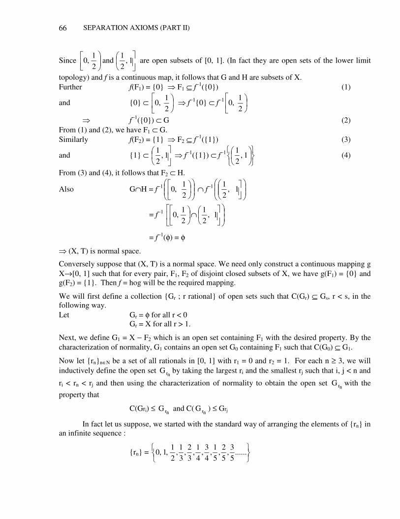
SEPARATION AXIOMS (PART II)

66

Since

1,21

and21

,0 are open subsets of [0, 1]. (In fact they are open sets of the lower limit

topology) and f is a continuous map, it follows that G and H are subsets of X. Further f(F1) = 0 F1 ⊆ f−1(0) (1)

and 0 ⊂

21

,0 f−10 ⊂ f−1

21

,0

f−1(0) ⊂ G (2) From (1) and (2), we have F1 ⊂ G. Similarly f(F2) = 1 F2 ⊆ f−1(1) (3)

and 1 ⊂

1,21

f−1(1) ⊂ f−1

1,21

(4)

From (3) and (4), it follows that F2 ⊂ H.

Also G∩H = f−1

21

,0 ∩ f−1

1,21

= f−1

∩

1,21

21

,0

= f−1(φ) = φ

(X, T) is normal space.

Conversely suppose that (X, T) is a normal space. We need only construct a continuous mapping g X→[0, 1] such that for every pair, F1, F2 of disjoint closed subsets of X, we have g(F1) = 0 and g(F2) = 1. Then f = hog will be the required mapping.

We will first define a collection Gr ; r rational of open sets such that C(Gr) ⊆ Gs, r < s, in the following way. Let Gr = φ for all r < 0 Gr = X for all r > 1.

Next, we define G1 = X − F2 which is an open set containing F1 with the desired property. By the characterization of normality, G1 contains an open set G0 containing F1 such that C(G0) ⊆ G1.

Now let rnn∈N be a set of all rationals in [0, 1] with r1 = 0 and r2 = 1. For each n ≥ 3, we will inductively define the open set

nrG by taking the largest ri and the smallest rj such that i, j < n and

ri < rn < rj and then using the characterization of normality to obtain the open set nr

G with the property that

C(Gri) ≤ nr

G and C(nr

G ) ≤ Grj

In fact let us suppose, we started with the standard way of arranging the elements of rn in an infinite sequence :

rn =

......

53

,52

,51

,43

,41

,32

,31

,21

,1,0

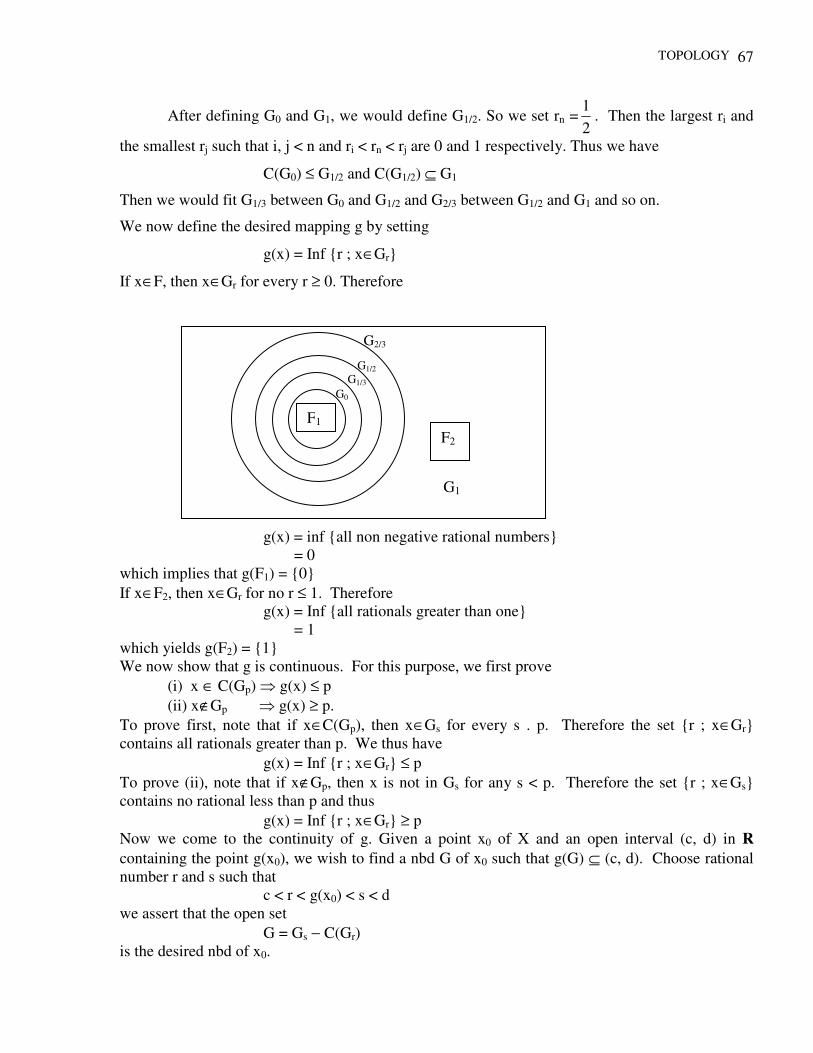
TOPOLOGY 67

After defining G0 and G1, we would define G1/2. So we set rn =21

. Then the largest ri and

the smallest rj such that i, j < n and ri < rn < rj are 0 and 1 respectively. Thus we have

C(G0) ≤ G1/2 and C(G1/2) ⊆ G1

Then we would fit G1/3 between G0 and G1/2 and G2/3 between G1/2 and G1 and so on.

We now define the desired mapping g by setting

g(x) = Inf r ; x∈Gr

If x∈F, then x∈Gr for every r ≥ 0. Therefore

g(x) = inf all non negative rational numbers = 0 which implies that g(F1) = 0 If x∈F2, then x∈Gr for no r ≤ 1. Therefore g(x) = Inf all rationals greater than one = 1 which yields g(F2) = 1 We now show that g is continuous. For this purpose, we first prove (i) x ∈ C(Gp) g(x) ≤ p (ii) x∉Gp g(x) ≥ p. To prove first, note that if x∈C(Gp), then x∈Gs for every s . p. Therefore the set r ; x∈Gr contains all rationals greater than p. We thus have g(x) = Inf r ; x∈Gr ≤ p To prove (ii), note that if x∉Gp, then x is not in Gs for any s < p. Therefore the set r ; x∈Gs contains no rational less than p and thus g(x) = Inf r ; x∈Gr ≥ p Now we come to the continuity of g. Given a point x0 of X and an open interval (c, d) in R containing the point g(x0), we wish to find a nbd G of x0 such that g(G) ⊆ (c, d). Choose rational number r and s such that c < r < g(x0) < s < d we assert that the open set G = Gs − C(Gr) is the desired nbd of x0.

G2/3

G1

G1/2

G1/3

G0

F1

F2

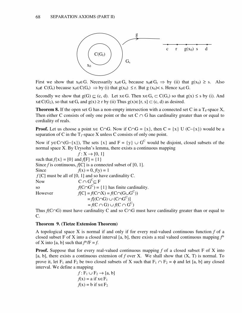
SEPARATION AXIOMS (PART II)

68

g

Gs

c r g(x0) s d First we show that x0∈G. Necessarily x0∈Gs because x0∉Gr by (ii) that g(x0) ≥ s. Also x0∉ C(Gr) because x0∈C(Gr) by (i) that g(x0) ≤ r. But g (x0)< s. Hence x0∈G.

Secondly we show that g(G) ⊆ (c, d). Let x∈G. Then x∈Gs ⊂ C(Gs) so that g(x) ≤ s by (i). And x∉C(G2), so that x∉Gr and g(x) ≥ r by (ii) Thus g(x)∈[r, s] ⊂ (c, d) as desired.

Theorem 8. If the open set G has a non-empty intersection with a connected set C in a T4-space X, Then either C consists of only one point or the set C ∩ G has cardinality greater than or equal to cordiality of reals.

Proof. Let us choose a point x∈ C∩G. Now if C∩G = x, then C = x U (C−x) would be a separation of C in the T1-space X unless C consists of only one point.

Now if y∈C∩(G−x), The sets x and F = y ∪ GC would be disjoint, closed subsets of the normal space X. By Urysohn’s lemma, there exists a continuous mapping f : X → [0, 1] such that fx = [0 and f[F] = 1 Since f is continuous, f[C] is a connected subset of [0, 1]. Since f(x) = 0, f(y) = 1 f [C] must be all of [0, 1] and so have cardinality C. Now C ∩ GC⊆ F so f(C∩GC) = 1 has finite cardinality. However f[C] = f(C∩X) = f(C∩(G∪GC)) = f[(C∩G) ∪ (C∩GC)] = f(C ∩ G) ∪ f(C ∩ GC) Thus f(C∩G) must have cardinality C and so C∩G must have cardinality greater than or equal to C.

Theorem 9. (Tietze Extension Theorem)

A topological space X is normal if and only if for every real-valued continuous function f of a closed subset F of X into a closed interval [a, b], there exists a real valued continuous mapping f* of X into [a, b] such that f*/F = f.

Proof. Suppose that for every real-valued continuous mapping f of a closed subset F of X into [a, b], there exists a continuous extension of f over X. We shall show that (X, T) is normal. To prove it, let F1 and F2 be two closed subsets of X such that F1 ∩ F2 = φ and let [a, b] any closed interval. We define a mapping f : F1 ∪ F2 → [a, b] f(x) = a if x∈F1 f(x) = b if x∈F2

C(Gr) x0

TOPOLOGY 69

This mapping is certainly continuous over the subspace F1 ∪ F2. Because if H be any closed subset of [a, b], then

f−1(H) =

∉∉∉∈∪

∉∈∉∈

Hbandhaif

HbandHaifFF

HaandHbifF

HbandHaifF

21

2

1

Since F1 and F2 are disjoint, we have (F1 ∪ F2) ∩ F1 = F1 and (F1 ∪ F2) ∩ F2 = F2

so that F1 and F2 are closed in F1 ∪ F2. Of course F1 ∪ F2 and φ are closed in F1 ∪ F2. Hence f is a continuous map over the subspace F1 ∪ F2. Hence by hypothesis, f can be extended to a continuous map g over X. This means that there exists a continuous map g : X→[a, b] such that g(x) = a if x∈F1 and g(x) = b if x∈F2

The mapping g now satisfies the condition stated in Urysohn’s lemma and hence (X, T) is normal.

Conversely let (X, T) be a normal space and let f be a real valued continuous map of the closed subset F into the closed interval [a, b] which for numerical convenience we take [−1, 1]. To show that there exist a continuous extension of f over X we begin by defining a map f0 : F→[−1, 1] by setting f0(x) = f(x) ∀ x∈F (1)

let G0 = f0−1

−−31

,1 , H0 = f0−1

1,31

Since

−− 1,31

and31

,1 are closed in [−1, 1] and f0 is continuous, it follows that G0 and H0

are closed in F and so also closed in X. Furthermore

G0 ∩ H0 = f0−1

∩

−− − 1,31

31

,1 10f

= f0−1

∩

−− 1,31

31

,1

= f0−1(φ) = φ

Thus G0, H0 are disjoint closed subsets of X. Since X is normal, from Urysohn’s lemma, we have a continuous map

g0 : X →

−31

,31

such that

g0[G0] =

=

−

31

)H(gand31

00

we next define a map

f1 : F →

−32

,32

by setting

SEPARATION AXIOMS (PART II)

70

f1(x) = f0(x) − g0(x) Since f0 and g0 are continuous, f1 is also a continuous map. Further, the range of f1 is contained in

−31

,32

as shown below:

If x∈G0, then

−1 ≤ f0(x) ≤ −31

and g0(x) = −31

so that

0 ≥ f0(x) − g0(x) ≥ −1 −

−31

i.e. 0 ≥ f0(x) − g0(x) ≥ −32

Similarly, if x∈H0, then

+31

≤ f0(x) ≤ 1 and g0(x) =31

so that

0 ≤ f0(x) − g0(x) ≤ 1−31

i.e. 0 ≤ f0(x) − g0(x) ≤ 32

Finally if, x∉G0 ∪ H0, then −31

< f0(x) <31

and −31

< g0(x) <31

, so that

−31

−31

< f0(x) − g0(x) <31

−

−31

that is −32

< f0(x) − g0(x) <32

Now let

G1 = f1−1

−−32

.31

,32

H1 = f1−1

32

,32

.31

Dealing with G1 and H1os we did with G0 and H0, we can show that G1 and H1 are disjoint closed subsets of X. By Urysohn’s lemma, there exists a continuous map

g1 : X →

−32

31

,32

31

such that

g1(G1) =

=

−32

.31

)H(gand32

31

11

we next define a map

f2 : F →

−22

32

,32

by setting

TOPOLOGY 71

f2(x) = f1(x) − g1(x) = f0(x) − g0(x) − g1(x) ∀ x∈F. As before, f2 is a continuous map whose range is contained in the closed interval

−22

32

,32

We continue the construction by induction. Suppose that for n = 0, 1, 2,…m−1, there exists a continuous map

gn : X →

−nn

32

31

,32

31

we define a map

fm : F →

−mm

32

,32

by setting

fm = f0(x) − −

=

1m

0ngn(x) ∀ x∈F

Now let

Gm = fm−1

−

−mm

32

31

,32

Hm = fm−1

mm

32

,32

31

Since

−

−mmmm

32

,32

31

and32

31

,32

are disjoint closed subsets of [−1, 1] and fm is continuous map. It follows that Gm, Hm are disjoint and closed in F as so also closed in X. Since Gm and Hm are disjoint closed subsets of normal space X, by Urysohn’s lemma, there exists a continuous map,

gm : X →

−mm

32

31

,32

31

such that

gm[Gm] =

−m

32

31

and gm [Hm] =

m

32

31

we define a mapping

fm+1 : F →

−++ 1m1m

32

,32

by setting

SEPARATION AXIOMS (PART II)

72

fm+1 = fm(x) − gm(x) = f0(x) − =

m

0ngn(x) ∀ x∈F

As in the case of f1 , It can be shown that fm+1 is a continuous map whose range in contained in

−++ 1m1m

32

,32

. Thus the induction is complete.

We now set

g(x) = ∞

=0ngn(x) ∀ x∈X

and show that g is continuous extension of f over X. We observe that

|g(x)| = | ∞

=0ngn(x)| ≤

∞

=0n |gn(x)| ≤

∞

=0n 31 n

32

= 13/21

3/1 =−

So by Weierstrass’s M−Test, the series ∞

0gn(x) converges uniformly and absolutely over X and

since gn(x) is continuous, it follows that g is a continuous mapping of X into [−1, 1]. Finally, we see that

|fm(x)| ≤m

32

→0 as m→∞.

Since fm(x) = f0(x) − −

=

1m

0ngn(x) ∀x∈F

we have

∞→m

lim fm(x) = f0(x) −∞→m

lim −

=

1m

0ngn(x)

Hence 0 = f0(x) − g(x) ∀ x∈F. that is, g(x) = f0(x) = f(x) ∀ x∈F by (1) It follows that g is a continuous extension of f over X.

Theorem 10. Every compact Hausdorff space is normal (T4).

Proof. Let F and F* be two disjoint closed subsets of the compact Hausdorff space X. Since F and F* are closed subsets of a compact space, they are also compact. Since the space is hausdorff, for each point <x, x*> of points with x∈F and x*∈F*, there exist disjoint open sets G(x, x*) and G*(x, x*) containing x and x* respectively. For each fixed point x∈F, the collection G*(x, x*) : x*∈F* forms an open covering of the compact set F*. Hence there must be a finite subcovering which we denote by G*(x, xi*) ; i = 1, 2,…,n Now let

G*(x) = Υn

1i=G*(x, xi*)

and G(x) = Ιn

1i=G(x, xi*)

Then G(x) and G*(x) are open disjoint sets containing x and F* respectively. Now the collection

TOPOLOGY 73

G(x) ; x∈F forms an open covering of the compact set F. There must be a finite subcovering, which we denote by G(xi) ; i = 1, 2,…m

If we let G = Υm

1i=G(xi) and the finite intersection. G* = Ι

m

1i=G*(xi), then G and G* are two disjoint

open sets containing F and F* respectively.

Theorem. 11. Every regular Lindeloff space is normal.

Proof. Let F and F* be two disjoint closed subsets of the regular Lindeloff space X. Since F and F* are closed subsets of a Lindeloff space they themselves are Lindeloff. Then for each x∈F, there exists an open set G(x) such that x∈G(x) ⊆ C(G(x)) ⊆ X−F* [Θ X−F* is open containing F] . The collection G(x); x∈F forms an open covering of the Lindeloff set F. There must be a countable subcovering which we denote by Gii∈N. Similarly, for each point x∈F*, there must exist an open set G*(x) such that x∈G*(x) ⊆ C(G*(x)) ⊆ X −F . The collection G*(x), x∈F* forms an open covering of the Lindeloff set F*. There must be a countable subcovering, which we denote by Gi*i∈N now the sets G = ΥΥ

nin

NnG[

≤∈− C(Gi*)]

and G* = ΥΥ

ni

*n

NnG[

≤∈− C(Gi)]

are disjoint open sets containing F and F* respectively. To show it, let Vn = Gn − Υ

ni≤C(Gi*)

and wn = Gn* − Υ

ni≤C(Gi)

Now Vn ∩ C(Gi*) = φ when i ≤ n. and wi ⊂ Gi* ⊂ C(Gi*) Hence Vn ∩ wi = φ when i ≤ n Similarly wj ∩ Vn = φ when n ≤ j Hence Vm ∩ wK = φ ∀ m, K ∈N Now Vn = Gn − UC(Gi*), i ≤ n = Gn ∩ [X−U C(Gi* ; i ≤ n)] It follows that Vn is an open set, being the intersection of two open sets.

Theorem 12. The property of a space being T4 is Hereditary.

Proof. Let (X, T) be a T4-space so that it is T1 as well as a normal space. Let (Y, T*) be a subspace of (X, T). We shall show that (Y, T*) is also a T4-space. Since the property of a space being T1 is hereditary, it follows that (Y, T*) is a T1-space. We now show that (Y, T*) is a normal space. Let L* and M* be two disjoint T* closed subsets of Y. If x is an arbitrary point of L* and y that of M*, then x ≠ y. Now x ≠ y. being degenerate (singleton) sets in T1 are disjoint T-closed subsets of X. Hence by normality of X, there exist T-open subsets Gx and Hy of X such that x ⊂ Gx, y ⊂ Hy and Gx ∩ Hy = φ These relations imply

SEPARATION AXIOMS (PART II)

74

L* ⊂ U(Gx; x∈L*, M* ⊂ UHy, y∈M and [UGx ; x∈L*] ∩ [UHy ; y∈M*] = φ set G = UGx ; x∈L*, H = U Hy, y∈M* then G and H are T-open subsets of X such that L* ⊂ G, M*⊂ H and G∩H = φ Since L* ⊂ Y and M* ⊂ Y, these relations imply L* C G∩Y, M*⊂H∩Y and (G∩Y) ∩ (H∩Y) = φ If we set G ∩ Y = G*, H ∩ Y = H* Then G*, H* are T*-open subsets of Y such that L*⊂G*, M* ⊂ H* and G* ∩ H* = φ which proves that (Y, T*) is normal also.

Theorem 13. Closed subspace of a normal space is normal. (Weakly- Hereditary)

Proof. Let (X, T) be a normal space and let (Y, T*) be a closed subspace of X. Let L*, M* be disjoint T* closed subsets of Y. Then there exist T-closed subsets L, M of X such that L* = L∩Y and M* = M∩Y

Since Y is T-closed, it follows that L*, M* are disjoint T-closed subsets of X. Then by normality of X, there exist T-open subsets G, H of X such that L* ⊂ G, M*⊂H and G∩H = φ since L*⊂Y and M* ⊂ Y, we have L* ⊂ G∩Y, M*⊂ H∩Y and (G∩Y) ∩ (H∩Y) = φ Setting G∩Y = G*, H∩Y = H*

We see that G* and H* are T*-open subsets of Y such that L* ⊂ G*, M* ⊂ H* and G* ∩ H* = φ. Hence (Y, T*) is normal.

Completely Normal Spaces Completely normal spaces were introduced by Tietz in 1923.

Definition. A topological space (X, T) is said to be completely normal if and only if it satisfies the following axiom of Tietz : “If A and B are two separated subsets of X, then there exist two disjoint open sets G and H such that A ⊂ G and B ⊂ H.

Definition. A completely normal space which is also T1 is called a T5-space.

Theorem 14. Every completely normal space is normal and hence every T5-space is a T4-space.

Proof. Let (X, T) be a completely normal space. Let A and B two closed subsets of X such that A ∩ B = φ. Since A and B are closed, we have C(A) = A, C(B) = B, and so C(A) ∩ B = φ, A∩C(B) = φ

Thus A and B are separated subsets of X. By complete normality, there exist open sets G and H such that A ⊂ G, B⊂H and G∩H = φ. It follows therefore that (X, T) is normal. Also definition, T5 is T1-space also. Therefore T5 is normal as well as T1-space also. Hence T5 is T4-space also.

Theorem. 15. Complete normality is a topological property

Proof. Let (X, T) be a completely normal space and let (Y, T*) be its homemorphic image under a homemorphism f. We shall show that (Y, T*) is completely normal. Let A and B be any two separated subsets of Y such that

TOPOLOGY 75

A∩C(B) = φ, B∩C(A) = φ. Since f is continuous mapping, we have C[f−1(A)] ⊂ f−1[C(A)] and C[f−1(B)] ⊂ f−1[C(B)] Hence f−1(A) ∩ C[f−1(B)] ⊂ f−1(A) ∩ f−1[C(B)] = f−1[A∩C(B)] = f−1(φ) = φ and C[f−1(A)] ∩ f−1(B) ⊂ f−1[C(A)] ∩ f−1(B) = f−1 [C(A) ∩ B] = f−1(φ) = φ

Thus f−1(A) and f−1(B) are two separated subsets of X. Since (X, T) is completely normal, there exist T-open sets G and H such that f−1(A) ⊂ G, f−1(B) ⊂ H and G∩H = φ These relations imply that A = f[f−1(A)] ⊂ f(G) B = f[f−1(B)] ⊂ f(H) (Θ of onto) and f(G) ∩ f(H) = f(G∩H) = f(φ) = φ [Θf is 1−1]

Also since f is an open map, f(G) and f(H) are T*-open sets. Thus we have shown that for any two separated subsets A, B of Y, there exist T* open subsets G1 = f(G) and H1 = f(H) such that A ⊂ G1, B ⊂ H1 and G1 ∩ H1 = φ which completes the proof of the theorem.

Corollary. The property of a space being T5-space is a topological property.

Proof. Since the property of a space being a T1-space and of being a completely normal space both are topological, it follows that the property of a space being a T5-space is also topological.

Theorem 16. Complete normality is a Hereditary property.

Proof. Let (X, T) be a completely normal space and (Y, T*) be any subspace of (X, T). We shall show that (Y, T*) is also completely normal. Let A, B be T*-separated subsets of (Y, T*), we have A ∩ C*(B) = φ and B∩C*(A) = φ Also C*(A) = C(A) ∩ Y and C*(B) = C(B) ∩Y Hence φ = A ∩ C*(B) = A∩[C(B)∩Y] = (A∩C(B)∩Y = A∩C(B) (i) Similarly φ = B ∩ C*(A) = B∩[C(A)∩Y] = (B∩C(A)∩Y = B∩C(A) (ii) So A and B are T-separated. Hence by completely normality of X, there exist T-open sets G and H such that A⊂G, B⊂H and G∩H = φ Since A and B are subsets of Y, A⊂G∩Y, B ⊂ H∩Y and (G∩Y) ∩ (H∩Y) = (G∩H) ∩Y = φ∩Y = φ It follows therefore that (Y, T*) is completely normal.

Cor. The property of a space being T5-space is a Hereditary property.

Proof. The property of a space being T1 as well as the property of a space being completely normal is hereditary. Therefore, it follows that the property of a space being T5 is hereditary.

SEPARATION AXIOMS (PART II)

76

Theorem. 17. A topological space X is completely normal if and only if every subspace of X is normal.

Proof. Let (X, T) be a completely normal space and (Y, T*) be any subspace of (X, T). We shall prove that (Y, T*) is normal. Let F1 and F2 be any pair of T* closed subsets of Y such that F1 ∩ F2 = φ. We shall denote the T* closure of F1 and F2 by C*(F1) and C*(F2) and their T-closure by C(F1) and C(F2) respectively. Since F1 and F2 are T*-closed, C*(F1) = F1 and C*(F2) = F2 Also C*(F1) = Y∩C(F1), C*(F2) = Y∩C(F2) Hence F1 ∩ C(F2) = C*(F1) ∩ C(F2) = (Y∩C(F1)) ∩ C(F2) = (Y∩C(F1)) ∩ (Y∩C(F2)) = C*(F1) ∩ C*(F2) = F1 ∩ F2 = φ Similarly F2 ∩ C(F1) = φ

It follows that F1 and F2 are two separated subsets of X. By complete normality there exist T-open sets G and H such that F1 ⊂ G. F2 ⊂ H and G∩H = φ. Then the sets G1 = Y∩G. and H1 = Y∩H are T* open sets such that F1 ⊂ G1, F2 ⊂ H1 and G1 ∩ H1 = (Y ∩G) ∩ (Y∩H) = Y ∩ (G∩H) = Y ∩ φ = φ (Y, T*) is normal.

Conversely suppose that (Y, T*) is normal. Let A and B by two separated subsets of X. Let Y = X−(C(A) ∩ C(B)). Then Y is T-open subset of X. The sets Y ∩C(A) and Y∩C(B) are T*−closed such that (Y∩C(A)) ∩ (Y∩C(B)) = Y ∩(C(A) ∩ C(B)) = [X−(C(A)∩C(B))] ∩ [C(A) ∩ C(B)] = φ Hence by the normality of Y, there exist T*-open subsets G, H of Y such that Y∩C(A) ⊂ G, Y∩C(B)⊂H (1) and G∩H = φ Again, since G and H are T*-open sets, there exist T-open sets G1 and H1 such that G = Y∩G1, H = Y∩H1 and since Y is T-open, it follows that G and H are also T-open sets. Further, since Y = X−[C(A)∩C(B)] and A and B are separated sets of X since Y = X − [C(A) ∩ C(B)] = [X −C(A)] ∪ [X−C(B)] But X−C(A) ⊃ B and X−C(B) ⊃A B ⊂ Y and A ⊂ Y. Hence it follows from (1) that A ⊂ G, B ⊂ H and G ∩H = φ (2) Also A and B are separated since B ⊂ X − C(A)

TOPOLOGY 77

Thus we have shown that for any pair A, B of separated subsets of X, there exist T-open subsets G and H satisfying (2). Hence (X, T) is completely normal.

Remark. Every completely normal space is normal but there are normal spaces which are not completely normal e.g. consider X = a, b, c, d T = φ, (a), (a, c), (a, b, c), X Here φ and X are the only disjoint closed subsets of X. Then (X, T) is normal. But the subspace Y = a, b, c of X is not normal as can be seen below If T* is a relative topology in Y which is given by T* = φ, (a), (a, b), (a, c), Y

Here (b) and (c) are disjoint T* closed subsets of Y but there are no disjoint open sets G and H such that (b) ⊂ G and (c) ⊂ H.

Hence the subspace (Y, T*) is not normal. It follows that the space (X, T) is not completely normal. This ex shows that normality is not hereditary.

Completely Regular Space and 213

T Space

Completely regular spaces were introduced by Paul Urysohn in a paper that appeared in 1925. Their importance was established by Tychonoff in 1930.

Definition. A topological space (X, T) is completely regular if and only if it satisfies the following axiom. “If F is a closed subset of X and x is a point of X not in F, then there exists a continuous mapping f : X→[0, 1] such that f(x) = 0 and f(x) = 1

Definition. A Tichonov space or

spaceT

21

3 is completely regular space which is also a

T1-space.

Theorem. 18. Every completely regular space is regular and hence every Tichonov space is a T3-space.

Proof. Let (X, T) be completely regular space. Let F be a closed subset of X and let x be a point of X not in F i.e. x∈X−F. By complete regularity there exists a continuous map f : X→[0, 1] such that such that f(x) = 0 and f(F) = 1. Also [0, 1] with relativised usual topology is a Hausdorff space. Hence there exist open sets G and H of [0, 1] such that 0∈G and 1∈H and G∩H = φ Since f is continuous, f−1(G) and f−1(H) are T-open subsets of X such that f−1(G) ∩ f−1(H) = f−1[G∩H] = f−1[φ] = φ Further f(x) = 0∈G x∈f−1(G) and f(F) = 1 ∈H F ⊂ f−1(H)

Thus there exist disjoint T-open sets f−1(G) and f−1(H) containing x and F respectively. It follows that (X, T) is regular. Also since every Tychonov space is a completely regular and T1-space, if follows that every Tychonov space is a T3-space.

Theorem. 19. Every T4-space is a Tychonov space. T4 21

3T .

SEPARATION AXIOMS (PART II)

78

Proof. Let (X, T) be a T4-space. Then by definition, it is normal and T1-space. Hence it sufficies to show that (X, T) is completely regular. Let F be a T-closed subset of X and bet x be a point of X such that x∉F. Since the space is T1, x is a closed subset of X. Thus x and F are closed subsets of X. Again since the space is normal, by Urysohn’s lemma, there exists a continuous mapping f : X→[0, 1] such that f[(x)] = 0 and f(F) = 1 i.e. f(x) = 0 and f(F) = 1.

Cor. Every compact Hausdorff space is a Tychonov space.

Proof. Since every compact Hausdorff space is normal, it is also Tychonov space.

Theorem 20. Complete regularity is a topological property.

Proof. Let (X, T) be a completely regular space and let (Y, V) be a homemorphic image of (X, T) under a homemorphism f. To show that (Y, V) is completely regular. Let F be a V-closed subset of Y and let y be a point of Y such that y∉F. Since f in one-one onto, there exists a point x∈X such that f(x) = y ⇔ x = f−1(y). Again since f is a continuous map, f−1(F) is a T-closed subset of X. Further y∉F f−1(y) ∉ f−1(F) x∉f−1(F). Thus f−1(F) is a T-closed subset of X and x = f−1(y) is a point of X such that x∉ f−1(F). Hence by complete regularity of X there exists a continuous mapping g of X into [0, 1] such that g[f−1(y)] = g(x) = 0 and g[f−1(F)] = 1 i.e. (gof−1) (y)) = 0 and (gof−1) (F) = 1

Since f is homemorphism, f−1 is a continuous mapping of Y onto X. Also g is a continuous map of X into [0, 1]. It follows that gof−1 is a continuous map of Y into [0, 1]. Thus we have shown that for each V-closed subset F of Y and each point y ∈Y−F, there exists a continuous map h = gof−1 of Y into [0, 1] such that h(y) = 0 and h(F) = 1. Hence (Y, V) is completely regular.

Remark. The property of a space being Tychonov space is a topological property.

Theorem. 21. Complete regularity is Hereditary property.

Proof. Let (X, T) be a complete regular space and let (Y, T*) be a subspace of X. Let F* be a closed subset of Y and y be a point of Y such that y∉F*. Since F* is T* closed, there exists a T-closed subset F of X such that F* = Y∩F. Also y∉F* y∉Y∩F y∉F [Θ y∈Y] and y∈Y y∈X.

This F is a T-closed subset of X and y is a point of X such that y∉F. Hence by complete regularity of X, there exists a continuous map f of X into [0, 1] such that f(y) = 0 and f(F) = [1

let g denote the restriction of f to Y. Then g is continuous mapping of Y into [0, 1]. Now by definition of g, g(x) = f(x) ∀ x∈Y. Hence f(y) = 0 g(y) = 0 and since f(x) = 1 ∀ x ∈F and F*⊂F, we have g(x) = f(x) = 1 ∀ x∈F* so that g(F*) = 1

TOPOLOGY 79

Thus we have shown that for each T*-closed subset F* of Y and each point y∈Y − F*, there exists a continuous map g of Y into [0, 1] such that g(y) = 0 and g(F*) = 1.

Remark. The property of a space being Tychonov is hereditary.

Theorem 22. A normal space is completely regular if and only if it is regular.

Proof. Since every completely regular space is regular, we only need to prove that any normal, regular space is completely regular. Let F be a closed subset of X not containing the point x so that x belongs to the open set X−F. Since the space X is regular, there exists an open set G such that x∈G and C(G) ⊂ X−F so that F ∩ C(G) = φ

Thus C(G) and F are disjoint closed subsets of a normal space X. Hence by Urysohn’s lemma, there exists a continuous mapping f : X → [0, 1] such that f(F) = 1 and f[C(G)] = 0 Also x∈G and f[C(G)] = 0 implies that f(x) = 0. Hence (X, T) is completely regular.

Example. Let (X, T) be a completely regular space. Prove that if F is a T-closed subset of X and p∉F, then there exists a continuous mapping f of X into [0, 1] such that f(p) = 1 and f(F) = 0.

Analysis. Since (X, T) is completely regular, there exists a continuous map g of X into [0, 1] such that g(p) = 0 and g(F) = 1

Now consider the mapping f : X → [0, 1] defined by setting f(x) = 1−g(x) ∀ x∈X. Since constant functions are continuous, it follows that f is continuous. Further )p(f = 1−g(p) = 1−0 = 1 f(x) = 1−g(x) = 1−1 ∀ x∈F = 0 so that f(F) = 0.

Example. Consider the topology T on R defined as follows T-consists of φ, R and all open says of the form [−∞, a) a∈R Show that (i) (R, T) is normal. (ii) Not regular (iii) Not T4 (iv) Is (R, T) complete regular.

Analysis. (i) Here the only disjoint closed subsets of R are of the form φ and [a, ∞) and for each such pair, there exist disjoint open sets φ and R such that φ ⊂ φ and [a, ∞) ⊂ R. It follows that (R, T) is normal.

(ii) Consider the closed set F = [1, ∞) and the point 0. Here 0∉F. But the only open set containing F is R which must intersect every open set containing zero. Hence there exists no open sets G and H such that 0∈G, F⊂ H and G∩H = φ. The space (R, T) is not regular.

(iii) The space (R, T) is not T1 since no singleton subset of R is T-closed. It follows that the space is not T4.

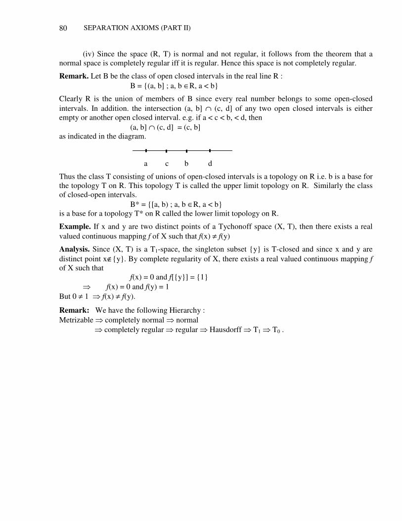
SEPARATION AXIOMS (PART II)

80

(iv) Since the space (R, T) is normal and not regular, it follows from the theorem that a normal space is completely regular iff it is regular. Hence this space is not completely regular.

Remark. Let B be the class of open closed intervals in the real line R : B = (a, b] ; a, b ∈R, a < b

Clearly R is the union of members of B since every real number belongs to some open-closed intervals. In addition. the intersection (a, b] ∩ (c, d] of any two open closed intervals is either empty or another open closed interval. e.g. if a < c < b, < d, then (a, b] ∩ (c, d] = (c, b] as indicated in the diagram. a c b d

Thus the class T consisting of unions of open-closed intervals is a topology on R i.e. b is a base for the topology T on R. This topology T is called the upper limit topology on R. Similarly the class of closed-open intervals. B* = [a, b) ; a, b ∈R, a < b is a base for a topology T* on R called the lower limit topology on R.

Example. If x and y are two distinct points of a Tychonoff space (X, T), then there exists a real valued continuous mapping f of X such that f(x) ≠ f(y)

Analysis. Since (X, T) is a T1-space, the singleton subset y is T-closed and since x and y are distinct point x∉y. By complete regularity of X, there exists a real valued continuous mapping f of X such that f(x) = 0 and f[y] = 1 f(x) = 0 and f(y) = 1 But 0 ≠ 1 f(x) ≠ f(y).

Remark: We have the following Hierarchy : Metrizable completely normal normal completely regular regular Hausdorff T1 T0 .

TOPOLOGY

81

6

EMBEDDING AND METRIZATION

Given a topological space (X, T), it is natural to ask whether there is a metric for X such that T is the metric topology. Such a metric metrizes the topological space and the space is said to be metrizable. Thus a metrizable space is a topological space whose topology is generated by some metric. There are topological spaces that are not metrizable for example let X be a set with atleast two members and let T be the trivial topology, then (X, T) is not metrizable.

Embedding

Definition. Let (X, T) and (Y, U) be topological spaces. An embedding or (sometimes called imbedding) of X into Y is a function e : X→Y which is a homemorphism when regarded as a function from (X, T) onto (e(X), U/e(X)) that is X is embedded in Y by f if and only if f is a homemorphism between X and some subspace of Y. Intuitively, to embed a space X into a space Y should mean that we can identify X with a subspace of Y, where identification is upto a homemorphism.

Example. The function f : R→R2 defined by f(x) = (x, 0) for each x∈R is an embedding of R in R2.

Analysis. It is clear that f is one to one. Let T denote the usual topology on R2 and let A = (x, y) ∈R2, y = 0. Then f maps R onto A. Since every metric space is first countable. In order to show that f is continuous, it is sufficient by the result that “Let f be a mapping of the first axiom space X into the topological space X*. Then f is continuous at x∈X if and only if for every sequence <xn> of points in X converging to x, we have the sequence <f(xn) converging to the point f(x) ∈X* ” Now to show that if <xn> is a sequence in R that converges to x in R. Then <f(xn)> converges to f(x) in A, is obvious. Thus f−1 is continuous. So if U denotes the usual topology on R, then f : (R, µ) → (A, TA) is a homemorphism

Remark. 1. If X is a subspace of a space Y, then the inclusion map i : X→Y defined by i(x) = x for every x∈X is an embedding. Thus inclusion maps are the most immediate examples of embeddings and as the definition implies, these are the only examples upto homemorphisms. An important problem in topology is to decide when a space X can be embedded in another space Y that is when there exists an embedding from X into Y. This is called the embedding problem. Theorems asserting the embeddability of a space into some other space which is more manageable than the original space are known as embedding theorems.

Theorem 1. Since a continuous bijection from a compact space onto a Hausdorff space is a homemorphism, every continuous, one to one function from a compact space into a Hausdorff space is an embedding.

Theorem 2. A function e : X→Y is an embedding if and only if it is continuous and one to one and for every open set V in X, there exists an open subset W of Y such that e(V) = W∩Y.

Proof. The result follows directly from definitions of homemorphism and relative topology.

EMBEDDING AND METRIZATION

82

Definition. Let Yi ;i∈I be an indexed family of sets. Suppose X is a set and let for each i∈I, fi : X→Yi be a function. Then the function e : X→ ∏

∈IiiY defined by e(x) (i) = fi(x) for i∈I, x∈X

is called the evaluation function of the indexed family fi ; i∈I of functions.

In other words, for each x∈X, the i-th co-ordinate of e(x) is obtained by evaluating the i-th function of fi at x. This justifies the term evaluation function. Intuitively evaluation function is obtained by listing together the information given by various fi’s. To illustrate this, suppose X is the set of all students in a class and f1, f2, f3,…, etc. are functions specifying respectively say, the age, the sex, the height etc of members of X. Then the evaluation function is like a catalogue which lists against each student all the information available about the student. For example, a typical entry in this catalogue might be

e(Mr. X. Y. Z) = (21, Male, 5 feet 6 inches,….) The following Theorem Characterizes evaluation functions.

Theorem 3. Let Yi ; i∈I be a family of sets, X, a set and for each i∈I, fi : X→Yi, a function then the evaluation function is the only function from X into Π Yi whose composition with the projection πi : Π Yi→Yi equals fi for all i∈I.

Proof. Let e : X→ΠYi be the evaluation function of the family fi ; i∈I. Then for any i∈I by very definition of e πi(e(x)) = e(x) (i) = fi(x) and so πi oe = fi .

Conversely, suppose e′ : X→Π Yi satisfies that πi o e′ = fi for all i∈I. Let x∈X. Then for any i∈I, e′(x) (i) = πi (e′(x)) = fi(x′) = e(x) (i)

and so e(x) = e′(x). But since x∈X was arbitrary, this means that e′ = e. Thus e is the only function from X into ΠYi having the given property.

Theorem 4. The evaluation function defined above is continuous if and only if each fi is continuous.

Proof. By the above prop, we have πi o e = fi for all i∈I.

Now by the result “Let (X, T) be the topological product of an indexed family of topological spaces (Xi, Ti) ; i∈I and let Y be any topological space. Then a function f : Y→X is continuous with respect the product topology on X if and only if for each i∈I, the composition πiof : y→Xi is continuous, where πi : X→Xi is the projection function”. The evaluation map is continuous if and only if each fi is continuous since projection mapping is always continuous.

Definition. An indexed family of functions fi : X→Yi ; i∈I where X, Yi are topological spaces, is said to distinguish points from closed sets in X if for any x∈X and any closed subset C of X not containing x, there exists j∈I such that fj (x) ∉ fj(C) in Yj.

This definition reminds us of complete regularity because there too, a point was separated from a closed set by means of a real valued map as the next theorem shows.

Theorem 5. A topological space is completely regular iff the family of all continuous real valued functions on it distinguishes points from closed sets.

Proof. Let X be a topological space and let F be the family of all continuous real valued functions on X. Suppose first that X is completely regular. Let a point x∈X and a closed subsets C of X, not containing x be given. Then there exists a continuous function f : X→[0, 1] such that f(x) = 0

TOPOLOGY

83

and f(C) ⊂ 1. Then we can regard f as a function from X to R. Then f ∈F and evidently f(x) ∉ )C(f since 1 is a closed subset of R. So F distinguishes points from closed sets in X.

Conversely suppose that F distinguishes points from closed sets. Let x∈X and C be a closed subset of X not containing x. Then there exists a map f : X→R such that f(x) ∉ )C(f . Now f(x)

and )c(f are disjoint closed subsets of R which is normal space. So there exists a continuous function g : R→[0, 1] which takes the values, 0 and 1 respectively on them. Let h : X→[0, 1] be the composite gof. Then clearly h(x) = 0 and h(y) = 1 for all y∈C. Thus X is a completely regular space.

Theorem. (Embedding Lemma) Let fi ; X→Yi ; i∈I be a family of continuous functions which distinguishes points and also distinguishes points from closed sets. Then the corresponding evaluation map is an embedding of X into the product space ∏

∈IiiY . To prove this result, first we

need to prove some Lemmas.

Lemma 1. The evaluation function of a family of functions is one-to-one if and only if that family distinguishes points.

Proof. For i∈I, let fi : X→Yi be a function, and let e : X→Π Yi be the evaluation function. Let x, y be distinct points of X. Then e(x) ≠ e(y) if and only if there exists j∈I such that e(x) (j) ≠ e(y)(j). But e(x) (j) = fj(x) by definition of e. Similarly e(y)(j) = fj(y).

So the condition that e(x) ≠ e(y) is equivalent to saying that there exists j∈I (which may depend upon both x and y) such that fj(x) ≠ fj(y). Since x, y are arbitrary. Thus The evaluation function of a family of functions is one to one if and only if that family distinguishes points.

Lemma 2. Let fi ; X→Yi, i∈I be a family of functions which distinguishes points from closed sets in X. Then the corresponding evaluation function e : X→ ∏

∈IiiY is open. When regarded as a

function from X onto e(X).

Proof. Let V be an open subset of X. We have to show that e(V) is an open subset of e(X). A typical point of e(V) is of the form e(x) for some x∈V. Now X−V is a closed subset of X not containing x. So by the hypothesis, there exists j∈I such that fj(x)∉ )VX(j −f . Let

G = Yj − )VX(j −f . Then G is an open subset of Yj and so 1j−π (G) is an open subset of ∏

∈IiiY we

claim that

1j−π (G) ∩ e(X) C e(V)

For suppose y∈ 1j−π (G) ∩e(X). Then y = e(z) for some z∈X. Also πj(y)∈G and so πj(e(z))∈G

whence fj(z) ∈G since πjoe = fj. From this it follows that z∈V, since otherwise fj(z)∈fj(X−V) ⊂ )VX(j −f = Yj − G. Thus y = e(z)∈e(V) as was to be shown. Now the set 1

j−π (G) ∩ e(X) is

open in the relative topology on e(X) and clearly it contains e(x), showing that e(V) is a neighbourhood of e(x) in e(X). But e(x) was a typical point of e(V). Then e(V) is a neighbourhood of each of its points in the relative topology on e(X). So e(V) is an open subset of e(X). Since this holds for all open sets V in X , we see that e, regarded as a function from X onto e(X) is open.

EMBEDDING AND METRIZATION

84

Remark. The converse of this lemma is false. Let X = R2 and f1, f2 be the two projections on R. Then the evaluation function is simply the identity map which is open. But the family f1, f2 does not distinguish points from closed sets in X.

Lemma 3. The evaluation function e : X→ ∏∈Ii

iY is continuous if and only if each fi : X→Yi is

continuous.

Proof. Already proved.

Proof of the theorem. Let e : X→ΠYi be the Lemma 3 evaluation function. Now continuity of the evaluation function e is continuous, follows from Lemma 3. That it is one to one follows from lemma 1 while lemma 2 shows that e is an open map when regarded as a function from X to e(X). Thus e is one to one, continuous and open from x to e(X). Hence e is an embedding.

Definition. The Cartesian product of closed unit intervals with the product topology is called a cube A cube is then the set I of all functions on a set A to the closed unit interval I with the topology of pointwise or co-ordinatewise, convergence. The cube is used as a standard sort of space and we want to describe those topological spaces which are homemorphic to subspaces of cubes.

Definition. The set I of all real sequences (a1, a2,…) such that 0 ≤ an ≤n1

for every n∈N is called

Hilbert cube. Also I is a closed and bounded subset of R∞

Tychonoff Embedding Theorem.

Theorem 7. A topological space is a Tychonoff space if and only if it is embeddable into a cube.

Proof. Let the topological space (X, T) be embedded into a cube. We shall prove that X is a Tychonoff space. Since we know that a Tychonoff space is T1 and completely regular and we know that every cube is a Tychonoff space. The Tychonoff property is Hereditary. So every subspace of a cube is Tychonoff. Also Tychonoff property is topological property, it is preserved under homemorphism. Thus every space homemorphic to a subspace of a cube is a Tychonoff space.

Conversely suppose X is a Tychonoff space. Let F be the family of all continuous functions from X into [0, 1]. Then since X is completely regular F distinguishes points from closed sets in X. But since X is also T1 all singletons are closed since we know that in a T1-space each singleton is closed. Thus it follows that F distinguishes points as well. But by the embedding lemma “Let fi ; X→Yi ; i∈I be a family of continuous functions which distinguishes points and also distinguishes points from closed sets. Then the corresponding evaluation map is an embedding of X into the product space ∏

∈IiiY ”. We have, the evaluation map e : X→[0, 1]F is an embedding of

X into the cube [0, 1]F.

Metrizability Definition :- A topological space (X, T) is metrizable if there is a metric d on X such that the topology induced by d is T .

Note the distinction between a metric space and metrizable space. A metrizable space is a topological space whose topology is generated by some metric and a metric space is a set with a metric on it. Of course the metric on a set X generates a topology on X and thus a metric space (X, d) determines a topological space (X, T). Given a metrizable space (X, T), there is a metric d

TOPOLOGY

85

on X such that the topology induced by d is T. As the metric d is not unique, there are many metrics that generate T.

Remark :- The following example shows that there are topological spaces that are not metrizable.

Example. Let X be a set with at least two members and let T be the trivial topology on X. Then (X, T) is not metrizable.

Analysis. Let d be a metric on X and let µ be the topology generated by d. We show that (X, T) is not metrizable by showing that µ ≠ T . Let a and b denote distinct members of X. By the definition of a metric, there is a positive number r such that d(a, b) = r. Therefore a ∈ B(a, r) but b ∉ B(a, r). Hence B(a, r) ∈ b, B(a, r) ≠ X and B(a, r) ≠ φ . But the only members of T are φ and X . Thus µ ≠ T .

Urysohn’s Metrization Theorem

Theorem 8. Every second axiom T3-space X is metrizable.

Proof. We shall show that any second axiom T3-space X is homemorphic to a subset of the Hilbert cube. Since Hilbert cube is metrizable. This will prove that X is metrizable.

Let Gnn∈N be the non-empty sets in some denumerable base for X, made infinite by repetition if necessary. Now for each integer j, there is some point x∈Gj and by regularity an open set G such that x∈G ⊆ C(G) ⊂ Gj. Since the collection Gn forms a base, there must be some integer i such that x∈Gi ⊆ G. Thus for every integer j, there is an integer i such that C(Gi) ⊆ Gj. The collection of all such pairs of elements from the base is denumerable and suppose <Gi, Gj> is the nth pair in some fixed ordering. The sets C(Gi) and X/Gj are then disjoint closed subsets of X. Since the regular second axiom space X is completely normal and hence normal. Thus by Urysohn’s Lemma, there exists some continuous mapping fn : X→[0, 1] such that fn (C(Gi)) = 0 and fn(X/Gj) = 1 .

We may define a mapping f of X into the Hilbert cube by setting f(x) = <2−n fn(x)>n∈N for every x ∈X.

Since 0 ≤ fn(x) ≤ 1 for all x∈X and integers n, f(x) is clearly a uniquely determined element of the Hilbert cube for each x∈X. We shall now show that f is a homemorphism of X onto f(X).

Let x and y be two distinct points of X. Since X is a T1-space, there exists some integer j such that x∈Gj but y∈X/Gj. As above there exists some integer i such that x∈Gi and C(Gi) ⊆ Gj. Suppose <Gi, Gj> is the nth pair in this ordering. The nth-coordinate of f(x) is 2−nfn(x) = 0. Since x∈C(Gi) while the nth-coordinate of f(y) is 2−n fn(y) = 2−n ≠ 0 since y∈X/Gj. Thus f(x) ≠ f(y) and f is one to one.

Also let x* be a fixed point of X and ∈ be arbitrary positive number. Let us choose first an index N = N(∈) such that

∞

+= 1Nn2−2n<∈2/2.

For each n, such that 1 ≤ n ≤ N, the mapping fn is continuous and so there exists a basic open set

Gn containing x* such that |fn(x*) − fn(x)| < N2

∈whenever x∈Gn .

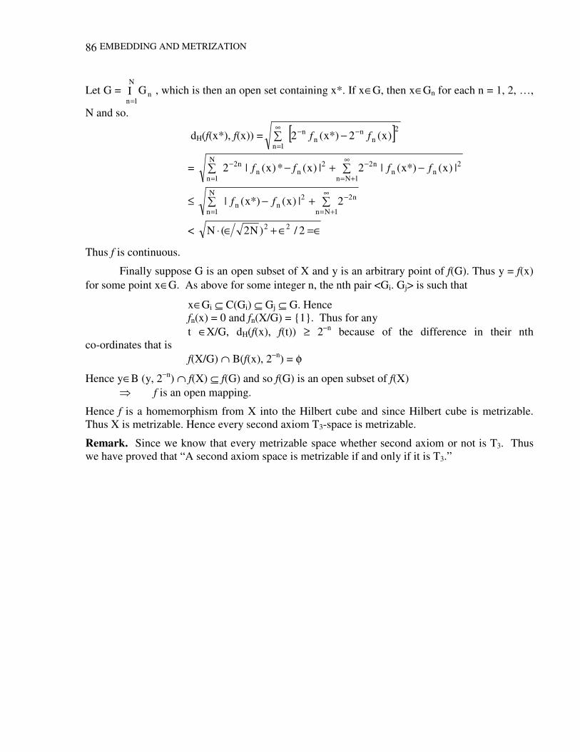
EMBEDDING AND METRIZATION

86

Let G = ΙN

1nnG

=, which is then an open set containing x*. If x∈G, then x∈Gn for each n = 1, 2, …,

N and so.

dH(f(x*), f(x)) = [ ]2nn

nn

1n)x(2*)x(2 ff −−∞

=−

= 2nn

n2

1Nn

2nn

n2N

1n|)x(*)x(|2|)x(*)x(|2 ffff −+−

−∞

+=

−

=

≤ n2

1Nn

2nn

N

1n2|)x(*)x( −∞

+==+− ff|

< =∈∈+∈⋅ 2/)N2(N 22

Thus f is continuous.

Finally suppose G is an open subset of X and y is an arbitrary point of f(G). Thus y = f(x) for some point x∈G. As above for some integer n, the nth pair <Gi. Gj> is such that

x∈Gi ⊆ C(Gi) ⊆ Gj ⊆ G. Hence fn(x) = 0 and fn(X/G) = 1. Thus for any t ∈X/G, dH(f(x), f(t)) ≥ 2−n because of the difference in their nth co-ordinates that is f(X/G) ∩ B(f(x), 2−n) = φ

Hence y∈B (y, 2−n) ∩ f(X) ⊆ f(G) and so f(G) is an open subset of f(X) f is an open mapping.

Hence f is a homemorphism from X into the Hilbert cube and since Hilbert cube is metrizable. Thus X is metrizable. Hence every second axiom T3-space is metrizable.

Remark. Since we know that every metrizable space whether second axiom or not is T3. Thus we have proved that “A second axiom space is metrizable if and only if it is T3.”

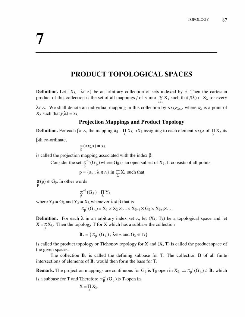
TOPOLOGY 87

7

PRODUCT TOPOLOGICAL SPACES

Definition. Let Xλ ; λ∈∧ be an arbitrary collection of sets indexed by ∧. Then the cartesian product of this collection is the set of all mappings f of ∧ into Υ

∧∈X such that f(λ) ∈ Xλ for every

λ∈∧. We shall denote an individual mapping in this collection by <xλ>λ∈∧ where xλ is a point of Xλ such that f(λ) = xλ.

Projection Mappings and Product Topology Definition. For each β∈∧, the mapping πβ :

λΠ Xλ→Xβ assigning to each element <xλ> of

Xλ its

βth co-ordinate,

βπ (<xλ>) = xβ

is called the projection mapping associated with the index β. Consider the set )G(1

β−

βπ where Gβ is an open subset of Xβ. It consists of all points

p = aλ ; λ ∈∧ in λΠ Xλ such that

βπ (p) ∈ Gβ. In other words

)G(1β

−

βπ =

λΠ Yλ

where Yβ = Gβ and Yλ = Xλ whenever λ ≠ β that is )G(1

β−βπ = X1 × X2 × …× Xβ−1 × Gβ × Xβ+1×….

Definition. For each λ in an arbitrary index set ∧, let (Xλ, Tλ) be a topological space and let X =

λπ Xλ. Then the topology T for X which has a subbase the collection

B∗ = )G(1λ

−βπ ; λ∈∧ and Gλ ∈Tλ

is called the product topology or Tichonov topology for X and (X, T) is called the product space of the given spaces. The collection B∗ is called the defining subbase for T. The collection B of all finite intersections of elements of B∗ would then form the base for T.

Remark. The projection mappings are continuous for Gβ is Tβ-open in Xβ )G(1β

−βπ ∈ B∗ which

is a subbase for T and Therefore )G(1β

−βπ is T-open in

X =λΠ Xλ.

PRODUCT TOPOLOGICAL SPACES

88

Theorem 1. Let A be a member of the defining base for a product space X =λΠ Xλ. Then the

projection of A into any co-ordinate space is open.

Proof. Since A belongs to the defining base for X. A =

λΠ Xλ ; λ ≠ α1, α2,…,αm ×

1G ×…×

mG where

iG is an open

subset of i

X . So for any projection πβ : X→Xβ,

πβ(A) =

∈

≠

...,,,ifG

...,,,ifX

m21

m21

In either case πβ(A) is an open set.

Theorem 2. Every projection πβ : X→Xβ on a product space X =Xλ is open.

Let G be an open subset of X. For every point p∈G, there is a member A of the defining base of the product topology such that p∈A⊂ G. Thus for any projection πβ : X→Xβ, p∈G πβ(p) ∈ πβ(A) ⊂ πβ(G)

But πβ(A) is an open set. Therefore every point πβ(p) in πβ(G) belongs to an open set πβ(A) which is contained in πβ(G). Hence πβ(G) is an open set.

Remark. As each projection is continuous and open, but projections are not closed maps e.g consider the space R×R with product topology. Let H = (x, y) ; x, y∈R and xy = 2 Here H is closed in R×R but π1(H) = R ~ (0)

is not closed with respect to the usual topology for R where π1 is the projection in the first co-ordinate space R.

Tychonov Product Topology in Terms of Standard Subbases Example. Consider the topology T = φ, X, (a), (b, c) on X = (a, b, c) and the topology T* = φ, Y, (u) on Y = (u, v) Determine the defining subbase B∗ of the product topology on X × Y.

Solution. X×Y = (a, u), (a, v) (b, u), (b, v), (c, u), (c, v)

is the product set on which the product topology is defined. The defining subbase B∗ is the class of inverse sets )H(and)G( 1

y1

x−− ππ where G is an open subset of X and H is an open subset of Y.

Computing, we have )Y()X( 1

y1

x−− ππ = X × Y,

1x−π (φ) = 1

y−π (φ) = φ

= (a, u), (a, v)

)c,b(1x−π = (b, u), (b, v), (c, u), (c, v)

)u(1y−π = (a, u), (b, u), (c, u)

TOPOLOGY 89

Hence the defining subbase B∗ consists of the subsets of X × Y above. The defining base B consists of finite intersections of members of the defining subbase that is B = φ, X × Y, (a, u), (b, u), (c, u) (a, u), (a, v), (b, u), (b, v), (c, u), (c, v) (a, u), (b, u), (c, u)

Theorem 3. Let (Xλ, Tλ) be an arbitrary collection of topological spaces and let X =λΠ Xλ. Let T

be a topology for X. If T is the product topology for X, then T is the smallest topology for X for which projections are continuous and conversely also

Proof. Let πλ be the λ-th projection map and let Gi be any Tλ-open subset of Xλ. Then since T is the product topology for X, )G(1

λ−λπ is a member of the subbase for T and hence )G(1

λ−λπ must be

T-open. It follows that πλ is T-Tλ continuous. Now let V be any topology on X such that πλ is V-Tλ continuous for each λ∈∧. Then )G(1

λ−λπ is V-open for every Gλ∈Tλ. Since V is a topology

for X, V contains all the unions of finite intersections of members of the collection )G(1

λ−λπ ; λ∈∧ and Gλ∈Tλ

V contains T that is T is coarser than V thus T is the smallest topology for X such that πλ is T−Tλ continuous for each λ∈∧.

Conversely. Let B∗ be the collection of all sets of the form )G(1λ

−λπ where Gλ is an open subset of

Xλ for λ∈∧. Then by definition, a topology V for X will make all the projections πλ continuous if and only if B∗ ⊂V. Thus the smallest topology for X which makes all the projections continuous, is the topology determined by B∗ as a subbase.

Theorem 4. A function f : Y→X from a topological space Y into a product space X =Xλ is

continuous if and only if for every projection πβ : X→Xβ, the composition mapping πβof : Y→Xβ is continuous.

Proof. By the definition of product space, all projections are continuous. So if f is continuous, then πβof being the composition of two continuous functions, is also continuous.

On the other hand, suppose every composition function πβof : Y→Xβ is continuous. Let G be an open subset of Xβ. Then by the continuity of πβof, (πβof)−1(G) = f−1 )]G([ 1

−

is an open set in Y. But the class of sets of the form )G( 1− where G is an open subset of Xβ is the

defining subbase for the product topology on X. Since their inverses under f are open subsets of Y, f is a continuous function.

Remark. The projections πx and πy of the product of two sets X and Y are the mappings of X×Y onto X and Y respectively defined by setting πx (<x, y>) = x and πy(<x, y>) = y

Theorem 5. If X and Y are topological spaces, the family of all sets of the form V×W with V open in X and W open in Y is a base for a topology for X×Y.

Proof. Since the set X×Y is itself of the required form, X×Y is the union of all the members of the family. Now let <x, y>∈ (V1 × W1) ∩ (V2 × W2) with V1 and V2 open in X and W1 and W2 open in Y. Then

PRODUCT TOPOLOGICAL SPACES

90

<x, y>∈ (V1 ∩ V2) × (W1 × W2) = (V1 × W1) ∩ (V2 × W2) with V1 ∩ V2 open in X and W1 ∩ W2 open in Y. Then the family is a base for topology for X×Y.

Theorem 6. Let Ci be a closed subset of a space Xi for i∈I. Then ∏∈Ii

iC is a closed subset of

∏∈Ii

iX w.r.t the product topology.

Proof. Let X = ∏∈Ii

iX and C = ∏∈Ii

iC . We claim X − C is an open set in the product topology on X

let x∈X−C. Then C = ΙIi

i1

i )C(∈

− and so x∉C implies that there exists j∈I such that πj(x) ∉ Cj. Let

Vj = Xj − Cj and let V = )V( j1

j− . Then Vj is an open subset of Xj and so V is an open subset (in

fact a member of the standard subbase) in the product topology on X. Evidently πj(x) ∈ Vj and so x∈V. Moreover C∩V = φ since πj(C) ∩ πj(V) = φ. So V ⊂ X − C. Thus X−C is a neighbourhood of each of it point. So X−C is open and C closed in X.

Separation Axioms and Product Spaces

In this section, we shall be concerned with finding out whether a certain topological property carries over from co-ordinate spaces to their topological products. In other words, suppose X is the topological product of an indexed family (Xi, Ti), i∈I of topological spaces. If each Xi has a topological property can we say that X also has it? This will depend upon the property itself and also upon how large the index set I is depending on it.

Theorem 7. Let X be topological product of an indexed family of spaces (Xi, Ti); i ∈ I. If the product is non-empty, then each co-ordinate space is embeddable in it.

Proof. Let X be the topological product of an indexed family of spaces (Xi, Ti) ; i∈I. Since X is non-empty, so in each Xi for i∈I. Now fix j∈I. We want to show that Xj can be embedded into X. For each j ≠ i in I, fix some yi∈Xi. Now define e : Xj→X by

e(x)(i) =

=∈≠

jiforx

Ijiforyi

In other words, e(x) is that element of ∏∈Ii

iX whose jth co-ordinate is x and all other co-ordinates

are equal to the respective chosen yi’s. Evidently e is one to one since e(x) = e(x′) would in particular imply e(x) (j) = e(x′) (j) whence x = x′.

Also the composite map πjoe is the identity map on Xj while for any i ≠ j, πj oe is the constant map taking all point of Xj to yi. In either case the composite πioe is continuous for all i∈I. So by the result “A function f : Y→X from a topological space Y into a product space X = ∏

jjX is

continuous if and only if for every projection πβ : X→Xβ, πβof : Y→Xβ is continuous”, e is continuous. To show that e is an embedding, it only remains to show that e is open when regarded as a function from Xj onto e (Xj). Note that e(Xj) is the box [A box in the product space X = ∏

jjX is a subset B of X of the form ∏

∈IiiB such that Bi ⊂ Xi, i∈I, For J∈I, Bj is called the j-th

TOPOLOGY 91

side of the box B] ∏∈Ii

iY where Yj = Xj and Yi = yi for i ≠ j∈I. Now let V be an open subset of

Xj. It is then easy to show that

e(V) = 1j− (V) ∩ e (Xj) as each side equals the box ∏

∈IiiZ where

Zj = V and Zi = yi for i ≠ j ∈I. Now the set 1j− (V) is open in X and so e(V) is an open in e(Xj)

in the relative topology. Thus e is an embedding. Theorem 8. A topological product is T0, T1, T2 or regular if and only if each co-ordinate space has the corresponding property. Proof. Since all the properties T0, T1, T2 or regular are hereditary, now if X = ∏

∈IiiX , then each

co-ordinate space Xj is homeomorphic to a subspace of X by the last theorem. (i.e. by Theorem 7). So whenever X is T0, T1, T2 or regular, so will be each Xj .

Conversely, we first show that T2-property is productive (i.e. A topological property is said to be productive if whenever (Xi, Ti); i ∈ I is an indexed family of spaces having that property. The topological product ∏

∈IiiX also has it). Suppose Xi is a T2 space for each i ∈ I, and let X = Π Xi

Let x, y be distinct points of X. Note that x,y are both functions on the indexed set I and so to say that they are distinct means that they assume distinct values at some index. So there exists j ∈ I such that x(j) ≠ y(j) i.e. πj(x) ≠ πj(y) in Xj (where πj : X → Xj)j∈I . Since Xj is a Hausdorff space, there exists disjoint open sets U and V in Xj such that x ∈ U, y ∈ V. Now let G = πj

−1(U) , H = πj

−1(V).

Then G, H are open subsets of X. Also x ∈ G, y ∈ H and G ∩ H = φ showing that X is a Hausdorff space. Similar argument applies to show that T0 and T1 are productive properties. Now we prove the converse part for regularity i.e. we will prove that if indexed family (Xi, Ti)i∈I of spaces is regular, then the topological product X = ∏

∈IiiX is regular. Suppose each Xi is regular and

x ∈ X and C be a closed subset of X not containing x. Then X−C is an open set containing x . So there exists a member V of the standard base for the product topology such that x ∈ V and V ⊂ X − C. Let V = ∏

∈IiiV where each Vi is open in Xi and Vi = Xi for all i ∈ I except possibly for i = i1,

i2,…, in (say). Let ri

x = ri

π (x) for r = 1,2,…,n. So be regularity of each co-ordinate space, there

exists an open set ri

U in ri

X such that ri

x ∈ ri

U and ri

U ⊂ ri

V . For i ≠ i1, i2,…, in, let Ui = Xi and

consider the box U = ∏∈Ii

iU . Clearly U is an open set in X and x ∈ U. Also U is contained in the

box ∏∈Ii

iU which itself is contained in V. But the set ∏∈Ii

iU is closed in X and hence contains

U. Thus x ∈ U and U ⊂ X − C. Therefore U and X−U are mutually disjoint open subsets containing x and C respectively. This show that X is regular.

Remark. Normality is not a productive property; It is not even finitely productive (i.e. whenever Xi’s are normal, the topological product ∏

∈IiiX is not normal (I finite). However, complete

regularity is productive property as shown below.

PRODUCT TOPOLOGICAL SPACES

92

Theorem 9. Let S be a subbase for a topological space X . Then X is completely regular if and only if for each V ∈ S, and for each x ∈ V, there exists a continuous function f : X → [0, 1] such that f(x) = 0 and f(y) = 1 for all y ∉ V.

Proof. If X is completely regular, then certainly the condition holds for all open sets, and so in particular members of S. Conversely suppose each V ∈ S, satisfies the given condition. Let G be an open set in X and let x ∈ G. By definition of a subbase, there exist V1, V2,…, Vn ∈ S such that

x ∈ Ιn

1iiV

=⊂ G . For each i = 1, 2,…, n, we have a map fi : X → [0, 1] which vanishes at x and

takes the value 1 outside Vi . Define

f : X → [0, 1] by f(y) = 1−(1−f1(y)) (1−f2(y)) … (1−fn(y))

Clearly f is continuous and f(x) = 0 and f takes the value 1 outside Ιn

1iiV

=and hence outside G.

This proves that X is completely regular.

Theorem 10. A product of topological spaces is completely regular if and only if each co-ordinate space is so.

Proof. From Theorem 7, since each co-ordinate space is embeddable in the topological product, and the fact that complete regularity is a hereditary property, i.e. if the space is completely regular, then every subspace is also completely regular. Thus if the topological product X = ∏

∈IiiX is

completely regular, then each space Xi is completely regular.

Conversely suppose X = ∏∈Ii

iX where each Xi is completely regular. Let S = πj−1(Vj); j ∈ I, Vj

open in Xj be the standard subbase for the product topology and suppose x ∈ πj−1(Vj). Then πj(x)

∈ Vj and so by the complete regularity of Xj, there exists a map f : Xj →[0, 1] such that f(πj(x)) = 0 and f takes value 1 on Xj−Vj. Then the composite foπj : X → [0,1] vanishes at x and takes value 1 on πj

−1(Xj−Vj) i.e. on X−πj−1(Vj). Hence the condition of last theorem (i.e. Theorem 9) is satisfied

by every member of the subbase S. So X is completely regular.

Theorem 11. A topological product of spaces is Tychonoff if and only if each co-ordinate space is so.

Proof. Since by definition Tychonoff property means the combination of complete regularity with T1, the result follows by merely putting together Theorem 8 and Theorem 10.

Theorem 12. ∏

X is Hausdorff if and only if each space Xλ is Hausdorff.

Proof. Suppose each space Xλ is Hausdorff and let X = <xλ>λ∈∧ and Y = <yλ>λ∈∧ be two distinct points of ∏

X . Since X and Y are distinct, there must exist some index β such that xβ ≠ yβ.

Since Xβ is a Hausdorff space, there must exist disjoint open subsets Gx and Gy containing xβ and yβ respectively. Clearly the sets )G(and)G( y

1x

1

−− are disjoint open sets in the product space

containing X and Y respectively since the projection mapping πβ : ∏∈Ii

iX →Xβ is continuous.

Hence if Gx and Gy are two disjoint open sets in the Hausdorff space Xβ containing xβ and yβ, Then

TOPOLOGY 93

)G(and)G( y1x

1

−− are disjoint open sets in the product space containing X and Y respectively.

This proves that ∏

X is Hausdorff.

Conversely suppose that ∏

X is Hausdorff. We want to prove that each Xλ is Hausdorff. Since

the property of a space being Hausdorff is Hereditary, we shall show that each Xλ is homeomorphic to a certain subset of the product space. This will prove that each Xλ is hausdorff. To do so, let <zλ> be a fixed point in the product space. For each β, consider the subset Eβ of the product space consisting of all points <xλ> such that xλ = zλ if λ ≠ β, while xβ may be any point of Xβ. Now let f be a πβ restricted to Eβ. f is clearly one-to-one continuous mapping of Eβ onto Xβ (since the projections are continuous) we want to show that f is open.

Now a base for the open sets in the subspace Eβ is the family of intersection of Eβ with the basis elements for the product topology. But Eβ∩ ∏

Y is either empty or consists of points of Eβ for

which xβ ∈ Yβ. The image under f is then either empty or Yβ and so open in either case. Thus f is homeomorphism.

Connectedness Theorem 13. X×Y is connected if and only if X and Y are connected.

Proof. Suppose first that X×Y is connected. Since πx : X×Y → X is continuous and X×Y is connected. The projection mapping πx maps the connected space into connected space. Hence X is connected. Similarly the continuous image Y of X×Y which is connected, is connected. Hence if X×Y is connected, then X and Y are also connected.

Conversely suppose that X and Y are connected. We shall prove that X×Y is connected. Let <x, y> and <x*, y*> be any two points of X×Y. Consider the mappings f : x × Y→Y g : X × (y* → X defined by f(<x, y>) = y and g(<x*, y*>) = x*.

It can be shown that f and g are homeomorphisms. Since projections are continuous and open. It follows therefore that x×Y and X×y* are connected. They intersect in the point <x, y*>. Hence by the result “The union E of any family Cλ of connected sets having a non-empty intersection is a connected set”. Their union is a connected set which contains the two points <x, y> and <x*, y*>. Thus X×Y is connected.

Theorem 14. ∏

X is connected if and only if each Xλ is connected.

Proof. Suppose first that ∏

X is connected. Define πβ : ∏

X →Xβ. Since the projection

mapping is continuous and the continuous image of a connected set is connected. It follows that each Xλ is connected.

Conversely suppose that each Xλ is connected. To prove that ∏

X is connected, let C be a

component of the product space and let <zλ ; λ ∈∧> be a fixed point in the product space which

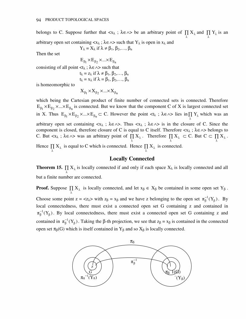
PRODUCT TOPOLOGICAL SPACES

94

1−

πβ

belongs to C. Suppose further that <xλ ; λ∈∧> be an arbitrary point of ∏

X and ∏

Y is an

arbitrary open set containing <xλ ; λ∈∧> such that Yλ is open in xλ and Yλ = Xλ if λ ≠ β1, β2,…, βn Then the set

n21E...EE ×××

consisting of all point <tλ ; λ∈∧> such that tλ = zλ if λ ≠ β1, β2,…, βn tλ = xλ if λ = β1, β2,…, βn is homeomorphic to

n21X...XX ×××

which being the Cartesian product of finite number of connected sets is connected. Therefore

n21E...EE ××× is connected. But we know that the component C of X is largest connected set

in X. Thus n21

E...EE ××× ⊂ C. However the point <tλ ; λ∈∧> lies in ∏

Y which was an

arbitrary open set containing <xλ ; λ∈∧>. Thus <xλ ; λ∈∧> is in the closure of C. Since the component is closed, therefore closure of C is equal to C itself. Therefore <xλ ; λ∈∧> belongs to C. But <xλ ; λ∈∧> was an arbitrary point of ∏

X . Therefore ∏

X ⊂ C. But C ⊂ ∏

X .

Hence ∏

X is equal to C which is connected. Hence ∏

X is connected.

Locally Connected Theorem 15. ∏

X is locally connected if and only if each space Xλ is locally connected and all

but a finite number are connected.

Proof. Suppose ∏

X is locally connected, and let xβ ∈ Xβ be contained in some open set Yβ .

Choose some point z = <zλ> with zβ = xβ and we have z belonging to the open set )Y( 1− . By

local connectedness, there must exist a connected open set G containing z and contained in )Y(

1− . By local connectedness, there must exist a connected open set G containing z and

contained in )Y( 1− . Taking the β-th projection, we see that zβ = xβ is contained in the connected

open set πβ(G) which is itself contained in Yβ and so Xβ is locally connected.

G πβ

−1(Yβ)

πβ

−1(G)

−(Yβ)

z

TOPOLOGY 95

Further, if z is any point of the product space, it must be contained in some connected open set G. By definition z∈ ∏

Y ⊆ G where Yλ is open in Xλ for all λ and Yλ = Xλ for all but a certain finite

number of values of λ. But then the projections of G are connected and are equal to Xλ, except for that finite number of values of λ.

Now suppose that Xλ is locally connected for old λ and connected for λ ≠ β1, β2,…, βn . Let X = <xλ>λ be an arbitrary point of ∏

Y where Yλ is open in Xλ for all λ and Yλ = Xλ for

λ ≠ β1*, β2*,…,βk*. Since xλ ∈Yλ for all λ and Yλ is locally connected, there is a connected open set Gλ in Xλ such that xλ∈Gλ ⊆ Yλ. Consider the subset ∏

Z where Zλ = Gλ if λ = β1, β2,…, βn,

β1*,…,βk* and Zλ = Xλ otherwise. But by the result “ ∏

X is connected if and only if each Xλ is

connected”. This set is connected. Hence we have formed a connected open set containing X and contained in ∏

Y .

Product Space as First Axiom Space

Theorem 16. Product space ∏

X is first axiom if and only if each space Xλ is first axiom and all

but a countable number are indiscrete.

Proof. Suppose ∏

X is first axiom. Since each space Xβ is homeomorphic to set Eβ where each

Eβ =

∏=><

β≠λ=><

λλλ

ββλλλ

XXofintpofixedaiszandXofintpoanyisxifzxthatsuchx

and the first axiom of countability is both hereditary and topological, each space is first axiom. Now if the space Xλ is not indiscrete, we may choose a point xλ∈Xλ which is contained in an open set Gλ ≠ Xλ. If Xλ is indiscrete, we choose any point xλ ∈ Xλ. Let X = <xλ> and suppose Bnn∈N is a countable open base at X. For each integer n, the set Bn must contain a member of the Tichonov base of the form ∏

Y where Yλ is open in Xλ for all λ and Yλ = Xλ for all but a finite number of

values of λ ; nnk

n2

n1 ,...,, . The collection of all the expected values of λ ; ; n

i i = 1, 2,…, kn and

n∈N is countable. For any other value of λ, we choose xλ∈Gλ ≠ Xλ if Xλ was not discrete, but 1− (Gλ) would then be an open set containing X which would not contain any Bn. Hence for all

other values of λ, Xλ must be indiscrete.

Now suppose that Xλ is first axiom for all λ and indiscrete for λ ∉λii∈N. Let X = <xλ>λ be an arbitrary point in ∏

X , and let Bn,λ be a countable open base at xλ. We note that Bn,λ = xλ for

all n if λ∉λi. The family 1i

− (Bn, λi), i, n∈N is a countable collection of open sets in the product space. The set of all finite intersections of members of this collection is also countable and it is already an open base at x, as desired.

PRODUCT TOPOLOGICAL SPACES

96

Product Space as Compact Space

Theorem 17. X×Y is compact if and only if X and Y are compact.

Proof. Since the projection mappings are continuous and onto if X ×Y is compact, then so are X and Y.

Conversely suppose that X and Y are compact. If G is any open covering of X×Y, then each member of G is a union of basis elements of the form V×W with V open in X and W open in Y. We may restrict our attention to the covering VλXWλλ∈∧ of X×Y by these basis elements where each Vλ×Wλ is contained in some member of G, since any finite subcovering of this basic open cover will lead immediately to a finite sub-covering chosen from the original cover G. For each x∈X, let Yx = x × Y which is homeomorphic to Y and hence compact. Since Vλ × Wλ also covers Yx , there must exist a finite subcovering n

1ii,xi;x WV =× of Yx by sets which have a non-empty intersection with Yx. Let

Gx = i,x

)x(n

1iVΙ

=

The Gx is an open set containing x and the above finite subcover actually covers Gx×Y. Now Gx ; x∈X covers X and so there is a finite subcover n

1jj,x G = . But then

n

1j

)jx(n

1ii,jxi,jx WV==

×

covers X×Y. Hence X×Y is compact.

Definition. Let X be any non-empty set. A filter H in the set X is a family of subsets of X satisfying the following axioms : (1) φ ∉ H (2) If F ∈ H, G ∈ H, then F ∩ G ∈ H . (3) If F ∈ H and H ⊃ F, then H ⊃ H.

Definition. An ultrafilter in a set X is a filter in X which is maximal in the collection of all filters

partially ordered by inclusion, that is a filter which is not properly contained in any other filter.

The topic will be discussed in detail in Chapter 8.

Theorem 18 (Tichonoff Product Theorem). Tλ Xλ is compact if and only each space Xλ is compact.

Proof. Since the projections are continuous, so if ∏λ

Xλ is compact, then each Xλ is compact.

Now suppose each Xλ is compact and let H be a family of closed subsets of ∏λ

Xλ with the finite

intersection property. The family H generates a filter which is contained in some ultrafilter F. Now consider the family

C iF(λπ ; F ∈ F

of closed subsets of Xλ . This family has the finite intersection property because

Ιn

1ii )F(C

=λπ ⊇ Ι

n

1ii )F(C

=λπ ⊇ Ι

n

1ii )F(

=λ∏

TOPOLOGY 97

which is nonempty because F has the finite intersection property. Now since Xλ is compact, there exists some point xλ which belongs to C( F

λπ ) for every F ∈ F . Let X = < xλ >λ and show that X

belongs to every set in F .

Now let S = ∏λ

Yλ with Yβ = Gβ an open set in Xβ and Yλ = Xλ if λ ≠ β be an arbitrary member of

the subbase for the product topology which contain X. But then Gβ is an open set containing the point xβ which is in the closure of

βπ F for every F ∈ F . Hence Gβ

must contain a point of βπ (F)

for every F ∈ F . Then S must contains a point of F for every F ∈ F and by the lemma, this implies that S ∈ F .

Finally let x be contained in an arbitrary open set G. By definition, x ∈ S1 ∩ … ∩ Sn ⊆ G for some finite number of sets Si in the subbase. We have just shown that each Si ∈ F and so S1 ∩ S2 ∩ Sn ∈ F and hence G ∈ F. Going back to our original family H of closed sets with the finite intersection property, we note that each member of H is also a member of F and so H ∩ G ∈ F for every H ∈ H and then H ∩ G ≠ φ for every H ∈ H . Thus x ∈ C(H) = H for every H ∈ H

ΙH∈H

H ≠ φ . So we have proved that every family of closed sets in the product topology which

has finite intersection property has a nonempty intersection. Thus ∏∧∈λ

λX is compact.

NETS AND FILTERS 98

8

NETS AND FILTERS

Inadequacy of sequences : We are familiar with the fact that a function f : R→R is continuous at x0 in R if whenever <xn> is a sequence converging to x0 in R, then the sequence <f(xn)> converges to f(x0). We introduced topologies for the purpose of providing a general setting for the study of continuous functions. Two questions arise. (a) Can we define sequential convergence in a general topological space ? (b) If so, does the resulting notion describe the topology and hence the continuous functions? The answer to the first question is yes and the definition is as follows :

Definition. A sequence <xn> in a topological space X is said to converge to x∈X written

∞→nlim xn = x or xn→x iff for each neighbourhood U of x, there is some positive integer n0 such that

xn∈U whenever n > n0. In this case we say that <xn> is eventually in U. A sequence is called convergent if and only if there is at least one point to which it converges.

The answer to the second question (b) is only for a limited class of spaces. In fact, we have

Theorem. 1. If <xn> is a sequences of distinct points of a subset E of a top space X which converges to a point x ∈ X then x is a limit point of the set E.

Proof. Proved earlier.

Remark. The converse of this is not true even in a Hausdorff space.

Theorem. 2. If f is a continuous mapping of the topology space X into a topology space X* and <xn> is a sequence of points of X which converges to the point x ∈ X, then the sequence <f(xn)> converges to the point f(x) ∈ X*.

Proof. Proved earlier.

Remark : The converse of this th is also not true even in a Hausdorff space. i.e. a mapping f for which xn→x implies f(xn)→f(x) may not be cont. However, the converse of the above theorems hold in the case of first axiom space and first countable space.

Theorem. 3. If X is first countable pace and E ⊂ X, Then x ∈E iff there is a sequence <xn> contained in E which converges to x.

Proof. Proved in Chapter IV.

Theorem 4. Let f be a mapping of the first axiom space X into topological space X*, then f is continuous at x∈X iff for every sequence <xn> of pts in X converging to x we have the sequence <f(xn)> converging to the point f(x) ∈ X*.

Proof. Proved in the Chapter IV.

TOPOLOGY

99

Remark. The failure of the converses of the theorems 1 and 2 show that the notion of limit for sequence of points is not completely satisfactory, even in the case of Hausdorff spaces. But these converses, as shown above in Theorem 3 and 4, may be proved if we take the first axiom space. Another way to obtain these results is to generalize the notion of sequence. This leads to the idea of Moore−smith sequence, Moore − Smith family, generalized sequence or a net. Still another approach is to consider the notion of a filter which we shall discuss later on.

Nets Definition. A set ∧ is a directed set iff there is a relation ≤ on ∧ satisfying

(a) λ ≤ λ for each λ∈∧

(b) λ1 ≤ λ2 and λ2 ≤ λ3 λ1 ≤ λ3.

(c) If λ1, λ2 ∈ ∧, then there is some λ3 ∈∧ with λ1 ≤ λ3 and λ2 ≤ λ3.

The relation ≤ is sometimes referred to as a direction on ∧ or is said to direct ∧ .

Remark. The first two properties (a) and (b) are well known requirement for an order relation. But the lack of antisymmetry shows that direction need not be a partial order. The concept of a net, which generalizes the notion of a sequence can now be introduced, using an arbitrary directed set to replace the integers.

Definition. A net in a set X is a function P : Λ→X. where Λ is some directed set. The point P(λ) is usually denoted by xλ and we often speak of the net <xλ>λ∈∧

or the net (xλ) if this can cause no confusion.

Example. 1. Every sequence is a net because (N, ≤) where ≤ is the usual ordering on N is a directed set.

Example. 2. The neighbourhood system Λx of a point x in a topological Space X is a directed set. Here for U, V∈ Λx, we define U ≤ V to mean U ⊃ V. (Note that this is in sharp contrast with our intuition that “U is smaller than V” should mean that U is contained in V). Conditions (a) and (b) hold trivally while (c) follows from the fact that the intersection of two neighbourhoods is again a neighbourhood. We define a net P : Λx→X now and denote P(U) by xU and thus <xU>U∈∧x is a net.

Example. 3. We give an example which is of historical significance in the definition of Riemann integrals. A partition of the unit interval [0, 1] is a finite sequence P = a0, a1,…, an such that 0 = a1 < a1 <…< an = 1. The interval [ai−1, ai], i = 1, 2,…, n is called the ith subinterval of P. Such a partition is said to be refinement of another partition Q = [b0, b1,…, bm] if each subinterval of P is contained in some subinterval of Q. Let us write P ≤ Q to mean that P is a refinement of Q. Then we see that ≤ directs the set of all partitions of [0, 1]. Conditions (a) and (b) of the definition are immediate. For (c) note that if P and Q are partitions, then the partition obtained by superimposing them together is a common refinement of P and Q. Let us define the Riemann net corresponding to a bounded − real valued function f on the unit interval [0, 1]. Let D be the set of all pairs (P, ξ) where ξ is a partition of [0, 1] say P = a0, a1,…, an and ξ = ξ1, ξ2, …, ξn is a finite sequence such that ξi ∈ [ai−1, ai] for i = 1, 2,…,n. Given two elements (P, ξ) and (Q, η) of D, let us say (P, ξ) ≤ (Q, η) iff P is a refinement of Q and for each j, ηj = ξi where i is so defined that the j−th subinterval of Q contained in the i-th subinterval of Q contained in the i-th subinterval of the partition P. It can be shown that ≤ directs D. Now define the net P : D → R by

P(P, ξ) = =

n

1if(ξi) (ai − ai−1)

NETS AND FILTERS 100

This is of course, nothing but what is called in the integral calculus as the Riemann sum of the function f for the partition P and the choice of points ξi in the ith subinterval of P and the Riemann integral as we know, is defined as the limit of such Riemann sums as the partitions gets more and more refined.

Example. 4. Let (M, ρ) be a metric space with x0∈M. Then M − x0 becomes a directed set when ordered by the relation x < y iff ρ(y, x0) < ρ (x, x0). Hence if f : M → N, where N is a metric space, the restriction of f to M −x defines a net in N.

Definition. A net P : Λ→X is eventually in X iff there is an element m of Λ such that if n ∈Λ and n ≤ m then P(n) ∈ X. This net is frequently in X iff for each m in Λ, there is n in Λ such that n ≤ m and P(n) ∈X.

Definition. Let (Λ, ≤) be a directed set. A subset M of Λ is said to be Cofinal subset of Λ if every α ∈ Λ, there exists ⊄ ∈M such that α ≤ ⊄. Clearly every eventual subset is a cofinal set but converse is not true.

For example, in N any infinite subset is cofinal but not necessarily eventual.

Topology and Convergence and Nets Definition. A net P : Λ→X is said to be eventually in a subset A of X iff the set P−1(A) is an eventual subset of A.

Definition. A net P : Λ→X is said to be frequently in a subset Λ of X if P−1(A) is a cofinal subset of Λ.

Definition. Let Λ and M be two directed sets. Then φ : M→Λ is said to be an increasing cofinal function if

(a) φ (µ1) ≤ φ(µ2) whenever µ1 ≤ µ2 (φ is increasing)

(b) For each λ ∈∧, there is some m ∈M such that

λ ≤ φ(m) (φ is cofinal in Λ)

Definition. A subnet of a net P : Λ→X is the composition P0φ where φ : M→ Λ is an increasing cofinal function from a directed set M to ∧.

For µ∈M, the point P0φ(µ) is often written as xλµ, and we usually speak of the subnet (xλµ) of (xλ).

Definition. If (xλ) is a net in X, a set of the form xλ ; λ ≥ λ0 for λ0 ∈ ∧, is called a tail of (xλ)

Definition. Let (xλ) be a net in the space X. Then (xλλλλ) is said to converge to x∈∈∈∈X, (written as xλ→x) if for every neighbourhood U of x, there exists λ0∈∧ such that λ ≥ λ0 implies xλ∈U.

Thus xλ→x if and only if each neighbourhood of x contains a tail of (xλ)

Sometime we say (xλ) converges to x provided it is residually or eventually) in every neighbourhood of x.

Definition. A point x∈X is said to be a cluster point of the net (xλ) if for every neighbourhood U of x and for each λ0 ∈∧, there exists some λ ≥ λ0 such that xλ ∈ U.

This is sometimes said (xλ) has x as a cluster point if and only if (xλ) is cofinally or frequently in each neighbourhood of x.

TOPOLOGY

101

Example. (1) We have seen in Ex 2 for the nets that we can define a net P : ∧x→X on the neighbourhood system ∧x of a point x∈X. We denote this net by (xU)U∈∧x. We observe that xU→x. Infact, given any neighbourhood V of x, we have U0 ≥ V for some U0 ∈∧x. Then U ≥ U0 ≥ V implies U ⊂ U0 so that x0 ∈ U0 ⊂ V.

(2) We know that every sequence is a net. The two definitions of convergence of (xn) coincide.

(3) We have seen in example 3 that

P(P, ξ) = =

n

1if(ξi) (ai − ai−1)

is a net. This sum is nothing but Riemann sum for the function f for the partition P and the choice of points ξi in the ith subinterval of the partition P. The Riemann integral is defined as the limit of this net (Riemann sum) as the partitions get more and more refined.

(4) We had seen in example 4, that the restriction of f : M→N to M − x, x∈M was a net in N. This net converge to z0 in N iff

0xxlim→

f(x) = z0 in the elementary calculus sense.

Remark. The definition of the cluster point of a net is a generalization of the notion of a limit point of a sequence. It is obvious that if a net (xλ) converges to x, then x is a cluster point of (xλ). Actually a stronger result holds.

Theorem 6. A net (xλ) has the point x as a cluster point if and only if it has a subnet which converges to x.

Proof. Let x be a cluster point of (xλ). Let M = (λ, U); λ∈∧; U is a neighbourhood of x containing xλ Define order ≤ in M as follows: (λ1, U1) ≤ (λ2, U2) iff λ1 ≤ λ2 and U2 ⊂ U1 we notice that (i) since λ1 ≤ λ1 (∧ being directed and U1 ⊂ U1, we have (λ1, U1) ≤ (λ1, U1) (ii) If (λ1, U1) ≤ (λ2, U2) and (λ2, U2) ≤ (λ3, U3) then λ1 ≤ λ2 and U2 ⊂ U1 and λ1 ≤ λ3 and U3 ⊂ U2 λ1 ≤ λ3 and U3 ⊂ U1 and thus we have (λ1, U1) ≤ (λ3, U3) (iii) If (λ1, U1) and (λ2, U2) ∈ M, then since ∧ is a directed set, there is a λ3∈∧ such that λ1 ≤ λ3, λ2 ≤ λ3. Moreover, U1 ∩ U2 ⊂ U1 as well as in U2. Then the pair (λ3, U1 ∩ U2) is the pair such that λ1 ≤ λ3 and U1 ∩ U2 ⊂ U1. i.e. (λ1, U1) ≤ (λ3, U1 ∩ U2) and also λ2 ≤ λ3 and U1 ∩ U2 ⊂ U2 i.e. (λ2, U2) ≤ (λ3, U1 ∧ U2) Thus ≤ is a direction on M. Define φ : M→∧ by φ(λ, U) = λ we have

φ(λ1, U1) = λ1

and φ(λ2, U2) = λ2

Therefore λ1 ≤ λ2 φ(λ1, U1) ≤ φ(λ2, U2) which shows that φ is increasing. Moreover if λ ∈ Λ, then there is some (µ, U) ∈ M such that λ ≤ φ(µ, U) = µ

NETS AND FILTERS 102

which shows that φ is cofinal in Λ. Therefore T = P oφ is a subnet of (xλ) we will now show that T converges to x ∈X. Let U0 be a neighbourhood of x in X. Since x is a cluster point of (xλ), the net (xλ) is frequently in U0. In particular fix any λ0 ∈ Λ such that

0xλ ∈ U0. Then (λ0, U0) ∈M.

Now for any (λ, U) ∈M, (λ, U) ≥ (λ0, U0) implies that U ⊂ U0, so that

T(λ, U) = Poφ(λ, U) = P(λ) = xλ∈U⊂U0.

Thus we have shown that for each neighbourhood U0 of x∈X, there exists (λ0, U0)∈M such that

(λ, U) ≥ (λ0, U0) T(λ, U) ⊂ U0

Hence the subnet T = Poφ of P is convergent to the limit x∈X.

Conversely suppose T = Poφ, where φ : M→∧ is a subset of P = (xλ) converging to x in X. Let U be any nbd of x in X and let λ0∈∧ be given. Since T converges to x, there exists µU in M such that for all µ∈M, µ ≥ µU implies T(µ) ∈U, i.e. P(φ(µ)) = xφ(µ)∈U.

Since φ(M) is cofinal in ∧, there is some u0∈M such that λ0 ≤ φ(u0). Choose µ*∈M such that µ* ≥ µ0 and µ* ≥ µU. Then φ(µ*) = λ* ≥ λ0. Since φ(µ*) ≥ φ(u0) ≥ λ0 and *)(x = xλ*∈U since µ* ≥

µ0. Thus for any neighbourhood U of x and any λ0∈∧, there is some λ* ≥ λ0 with xλ*∈U. It follows that x is a cluster point of (xλ).

Cor. If a subnet of (xλ) has x as a cluster point, so does (xλ).

Proof. A subnet of a subnet of (xλ) is a subnet of (xλ).

We turn now to the problem of showing that nets do indeed represent the correct way of approaching convergence question in topological spaces.

Theorem 6. If E⊂X, then x∈E (closure of E) if and only if there is a net (xλ) of points of E with xλ→x.

Proof. If x∈E, then each neighbourhood U of x, meets E in at least one point xU. We take the index set as the collection of all neighbourhoods of x ordered by reverse inclusion. Then

xUUU )x( ∈ is a net contained in E which converges to x. To show the convergence, let V be any

neighbourhood of x. We have U0⊂V for some U0∈Ux (since Ux represents the base of neighbourhoods). Then for all U ≥ U0 ≥ V we have

xU ∈ U0 ⊂ V . Hence xU→x.

Conversely if (xλ) is a net contained in E and xλ→x. Then every neighbourhood of x contains a tail of (xλ). Thus every neighbourhood of x meets E and hence x∈E.

Theorem 7. Let f : X → Y. Then f is continuous if and only if whenever xλ→x0 in X, then f(xλ)→f(x0) in Y.

Proof. Suppose f is continuous at x0. Therefore given a neighbourhood V of f(x0), f−1(V) is a neighbourhood of x0. Now let xλ→x0, therefore ∃ λ0 such that λ ≥ λ0 implies xλ∈ f−1(V). Thus λ ≥ λ0 implies f(xλ)∈V. This shows that f(xλ)→f(x0).

On the other hand, if f is a not continuous at x0, then for some neighbourhood V of f(x0), f(U) ⊄ V for any neighbourhood U of x0. Thus for each neighbourhood U of x0, we can pick xU∈U such that f(x0) ∉ V. But then (xU) is a net in X and xU→x0, while f(xU) →/ f(x0).

TOPOLOGY

103

Theorem 8. A net <xλ> in a product X = ∏∧∈

Xα converges to x if and only if for each α∈Λ,

πα(xλ) → πα(x) in Xα.

Proof. Let xλ→x in ∏∧∈

Xα. Since projection mapping πα is cont. by the above theorem, πα(xλ) →

πα(x) in Xα.

Suppose on the other hand, that πα (xλ) → πα(x) for each α∈Λ (index set). Let

11

−απ , (Uα1) ∩ …∩ παn

−1 (Uαn)

be a basic neighbourhood of x in the product space. Then for each i = 1, 2,…, n, there is a λi such that whenever λ ≥ λi, we have

iαπ (xλ) ∈ Uα. Thus if λ0 is picked greater than all of λ1, λ2…, λn

we havei

(xλ) ∈ Uαi, i = 1, 2, …,n for all λ ≥ λ0. It follows that for λ ≥ λ0, xλ∈ 1i

−απ (Uαi) and

hence xλ→x in the product.

Hausdorffness and Nets

Theorem 9. A topological space is Hausdorff if and only if limits of all nets in it are unique.

Proof. Suppose X is a Hausdorff space and P : ∧→X is a net in X. Let P converges to x and y in X. We have to show that x = y. If this is not so, then there exists open sets U and V such that x ∈U, y∈V and U∩V = φ. Since P converges to x, there exists λ1 ∈∧ such that for all λ∈Λ, λ1 ≥ λ, implies P(λ)∈U. Again since P converges to y, there exists λ2∈∧ such that for all λ∈∧, λ ≥ λ2 implies P(λ)∈V. Now because ∧ is a directed set, there exists λ∈∧ such that λ ≥ λ1 and λ ≥ λ2. But that P(λ)∈U, P(λ) ∈V i.e. P(λ) ∈ U∩V, a contradiction since U∩V = φ, so x = y, establishing the necessity of the condition.

Conversely suppose that the limits of all nets in a space X are unique. If X is not Hausdorff, then there exist two distinct points x, y in X which do not have mutually disjoint neighbourhood in X. Let µx and µy be the neighbourhood systems in X at x and y respectively. Let ∧ = µx × µy and for (U1, V1), (U2, V2) ∈∧, define (U1, V1) ≥ (U2, V2) if and only if U1 ⊂ U2 and V1 ⊂ V2. This makes ∧ a directed set and we define a net P : ∧→X as follows :

For any U∈µx and V∈µy we know that U ∩ V ≠ φ. Define P(U, V) to be any point in U ∩ V. We assert that the net P so defined converges to x. In fact, let G be any neighbourhood of x. Then (G, X)∈∧. Now if (U, V) ≥ (G X) in ∧ then U ⊂ G and so P(U, V) ∈ U ∩ V ⊂ U ⊂ G. This proves that P converges to x. Similarly we can show that P converges to y also contradicting the hypothesis. Hence X is a T2-space.

Remark. The proof of the converse illustrates the advantage nets have over sequences. In a sequence, the domain is always the set of positive integers, while in defining nets, we have considerable freedom in the choice of the directed set.

Compactness of Nets Definition. A family F of subsets of a set X is said to have the finite intersection property if for

any n∈N and F1 F2,…, Fn∈F, the intersection Ιn

1i=Fi is non-empty. In particular every member of

a family having finite intersection property is non-empty.

Prop. A topological space is compact if and only if every family of closed subsets of it, which has the finite intersection property, has a non-empty intersection. Now we can prove the following

NETS AND FILTERS 104

Theorem 10. For a topological space X, the following statements are equivalent (i) X is compact (ii) Every net in X has a cluster point in X. (iii) Every net in X has a convergent subnet in X (i.e. a subnet which converges to at least one point in X).

Proof. We have proved the equivalence of (i) and (ii) alreadby (by Theorem 5). Therefore, we only prove the equivalence of (i) and (ii). So we suppose that X is compact and let P : ∧→X be a net in X. Suppose X has no cluster point in X. Then for each x∈X, there exists a neighbourhood Nx of x and an element mx∈∧ such that for all n∈∧, n ≥ mx implies P(n)∈X−Nx cover X by such neighbourhoods (or more precisely, by their interiors). By compactness of X, there exist x1,

x2,…, xk ∈X such that X = ix

K

1iNΥ

=. Let the corresponding elements in ∧ be m1, m2,…, mk. Since

∧ is a directed set, there exists n∈∧ such that n ≥ mi for i = 1, 2,…, k. But then P(n)

∈ )NX(ix

K

1i−

=Υ = X −

ix

K

1iNΥ

== φ, a contradiction.

Hence P has at least one cluster point in X. Thus (ii) holds.

Conversely suppose that (ii) holds. Let C be a family of closed sets of X having the finite intersection property. Let D be the family of all finite intersections of members of C. D itself is closed under finite intersections and that C ⊂ D. For D, E ∈ D, we define D ≥ E to mean D ⊂ E. This makes D, a directed set because whenever D, E∈D, D ∩ E ∈D and D ∩ E ≥ D, D ∩ E ≥ E. Note that each member of D is non-empty because C is given to have the finite intersection property. So we can define a net P ; D→X by P(D) = any point in D. By (ii), this net has a cluster point say x in X. We claim x ∈ Ι

C∈⊂C. For if not, there exists C ∈ C such that x∉C. Then X − C

is a neighbourhood of x (since members of C are closed). Also C∈D. So by the definition of a cluster point, there exists D∈D such that D ≥ C and P(D) ∈ X − C. But then D⊂ C, and so X−C ⊂ X − D contradicting that P(D)∈D. So x ∈ Ι

C∈⊂C. We have thus shown that every family

of closed subsets of X having finite intersection property has non-empty intersection. But this implies that X is compact.

Definition. A net <xλ> in a set X is an ultranet (universal net) if and only if each subset E of X, (xλ) is either residually in E or residually in X−E.

It follows from this definition that if an ultranet is frequently in E, then it is residually in E. In particular, an ultranet in a topological space must converge to each of its cluster points.

For any directed set ∧, the map P : ∧→X defined by P(λ) = x for all λ∈∧, gives an ultranet on X, called the trivial ultranet. Non-trivial ultranets can be proved to exist (relying on the axiom of choice) but none has ever been explicitly constructed. Most facts about ultranets are best developed using filters at ultrafilters.

Theorem 11. If <xλ> is an ultranet in X and f : X→Y, then (f(xλ)) is an ultranet in Y.

Proof. If A ⊂ Y, then f−1(A) = X − f−1(Y − A) therefore by the definition of ultranet, <xλ> is eventually in either f −1(A) or f −1(Y − A) from which it follows that (<f(xλ(>)) is eventually in either A or Y−A. Thus (f(xλ)) is an ultranet.

Theorem 12. For a top. Space X, the following are equivalent.

TOPOLOGY

105

(a) X is compact. (b) Every net in X has a cluster point in X. (c) Every net in X has a convergent subnet in X. (d) Each ultranet in x converges.

Proof. We have already proved the equivalence of (a), (b) and (c). Moreover each ultranet is a net and by (b) it has a cluster point and hence converges to that point. Thus (b) (d). Similarly we can prove that (d) (b) thus these four statements will be equivalent.

Filters and Their Convergence We now introduce a second way of describing convergence in a topological space. The result is the theory of filter convergence.

Definition. A filter H on a set S is a non-empty collection of subsets of S such that. (a) φ ∉H (b) If F1, F2 ∈ H, then F1 ∩ F2 ∈ H (c) If F ∈ H and F′ ⊃ F, then F′∈H.

In view of the result “If a family B of subsets of a set X is closed under finite intersection, then B has finite intersection property”. It follows that the conditions (a) and (b) imply that a filter has the finite intersection property. Condition (c) says that a filter is closed under the operation of taking supersets of its members. It implies in particular that the set S always belongs to every filter on it.

Definition. Let H be a filter on a set S. Then a subfamily B of H is said to be filter base for H if for any F∈H, there exists G∈B such that G⊂F. Thus if B is a base for a filter H, then every members of H is a superset of some members of B.

On the other hand if B∈B, then B∈H and so nay subset of B is in H by condition (c) of the definition of a filter. Thus if B is a base for a filter H, then H consists precisely of all supersets of members of B, i.e.

H = F ⊂ S ; F ⊃ B, B ∈B

Definition. If H1 and H2 are filters on the same set x, we say H, is finer than H2 (or H2 is coarser than H1) if and only if H1 ⊃ H2.

Definition. Two filters H1 and H2 are said to be comparable if and only if H1 is finer than H2 or H2 is finer than H1.

Definition. A filter H on a set X is said to be fixed if and only if ∩ H ≠ φ, and fine if ∩ H = φ.

Remark. The set of all filters on X is directed by the relation ≤ defined by setting H1 ≤ H2 iff H2 is finer than H1.

Examples. (1) If X is any non-empty set, then the singleton family X is a filter on X. Moreover X is the coarset filter on X. In other words X is the smallest element of the ordered set of all filters on X. But there is no largest filter on X if X consists of more of more than one element as we will see later on. In fact among the families satisfying axioms (b) and (c), the power set P(X) is largest and it is excluded by axiom (a)

(2) Let X be any non-empty set and x0∈X. Then the family

H = F ; x0 ∈F

is a filter on X. To show it, we observe that H is non-empty since x0 ∈ H. Moreover

NETS AND FILTERS 106

(i) Since x0∈F for all F∈H, it follows that no member of H is empty and so φ ∉ H. (ii) Let F∈H H∈ H, then x0 ∈ F and x0 ∈ H. Thus x0 ∈ F ∩ H FAH ∈ H . (iii) Let F∈H and H ⊃ F. Then x0 ∈ F x0 ∈H H∈H. Hence H is a filter.

(3) Let F0 be a non-empty subset of a set X. Then the collection

H = F ⊂ X, F ⊃ F0

of all supersets of F0 (in X) is a filter on X. Such a filter is known as Atomic filter. The set F0 being called Atom of the filter. In this case, F0 is the intersection of all members of the filter. The filter base for this filter H is the collection consisting of the single set F0.

(4) Let X be any infinite set. Then the collection H = F ; X−F is finite.

of all cofinite subsets of X is a filter on X (Note that this filter is not atomic). Such a filter is called the cofinite filter. We prove it as follows

Since X − X = φ, is finite. X∈H and hence H is non-empty. Further

(i) Since X is infinite and X−F is finite, it follows that F is an infinite set and hence no member of H is empty. Thus φ∉H.

(ii) If F, H ∈H, then X−F and X−H are both finite. Now X − (F∩H) = (X−F) ∪ (X−H) (Demorgan’s Law)

Since (X−F) and (X−H) are finite, it follows that X−(F∩H) is finite F∩H∈H.

(iii) Let F∈H, and H ⊃ F. Since X−F is finite X −H is finite. Hence H∈H. Thus H is a filter.

(5) Suppose (X, T) is a topological space. Then for any x∈X, the neighbourhood system Ux at x is a filter. It is called the T-neighbourhood filter at x. Any neighbourhood base at x is a filter base for T-neighbourhood filter.

(6) Let N be the set of non-negative integers. Then the collection H = F ; N − F is finite Is a filter on N. This is known as Frechet Filter.

(7) Let P = ∧→X be a net. For each λ0∈∧, let

0B = P(λ) ; λ∈∧ ; λ ≥ λ0

let H = F ⊂ X ; F ⊃0

B for some λ0 ∈∧.

In other words, H is the collection of all supersets of the sets of the form 0

B ; λ0∈∧. Using the

fact that ∧ is a directed set, it can be shown that H is a filter on X. Obviously it depends on the net and is called the filter associated with the net P.

Theorem 13. Let Hλ be any non-empty family of filters o a non-empty set X (which must therefore be non-empty). Then the set H = ∩Hλ is also a filter on X.

Proof. We have (i) Since φ∉Hλ for any λ∈∧, if follows that φ∉H.

TOPOLOGY

107

(ii) Let F, H∈H. Then F∈Hλ, H∈Hλ for all λ∈∧. Since each Hλ is a filter it follows that F ∩ H ∈ Hλ for all λ ∈∧. Hence F ∩ H ∈H.

(iii) Let F∈H, H ⊃ F, then F ∈Hλ for all λ∈∧. Since each Hλ is a filter and F∈Hλ, it follows that H∈Hλ for all λ∈∧. Hence H∈H. Thus the theorem is proved.

The filter H = ∩Hλ constructed above is called the intersection of the family of filters Hλ and is obviously the greatest lower bound of the set of the Hλ in the ordered set of all filters on X.

Theorem 14. Let A be any non-void family of subsets of a set X. Then there exists a filter on X containing A if and only if A has finite intersection property.

Proof. Suppose first that A has finite intersection property. We have to show that there exists a filter on X containing A. Let B = B ; B is the intersection of a finite subfamily of A .

Since A has finite intersection property (f. i. p) no member of B is empty. Hence φ∉B. Now set

H = F ; F contains a member of B

Evidently H ⊃ A. We claim that H is a filter on X. In this direction, we have

(1) Since φ∉B and every member of H is a superset of some members of B, it follows that φ∉H.

(2) Let F∈H and H ⊃ F. Since F contains a member of B, H must also contain that member. Hence H∈H.

(3) Let F, H∈H. Then F ⊃B, H ⊃ C, where B and C are members of B. Since B and C are finite intersections of members of A. B ∩ C must also be a finite intersection of members of A. Hence B ∩ C ∈B. Also F ⊃ B, H ⊃C F ∩ H ⊃ B ∩ C. Thus F∩H contains a member of B and so F ∩ H ∈H.

Thus we have shown that if A has f. i. p, then ∃ a filter H containing A.

Conversely suppose that H is a filter on X containing A. Then H also contains the collection B of finite intersection of members of A. hence a necessary condition for the existence of such a filter H is that φ ∉ B, i.e. A must have f. i. p.

Cor. The filter H obtained above is the coarset filter which contains A i.e. the smallest element of the ordered family of all filters on X containing A.

In fact, if H′′′′ is any filter containing A, then H′′′′ must contain all finite intersections of members of A and their supersets and hence H′ ⊃H.

Definition. The filter H defined in the above theorem is said to be generated by A and A is said to be a subbase of H.

Observe that for A to be a subbase, it is necessary and sufficient that f has f. i. p.

Remark. The above theorem suggests the following method of constructing a filter.

Take any family A of subsets of X with f. i. p. Then obtain the family B of all finite intersections of A. The family H of all those subsets of X which contain a member of B is a filter on X e.g. X = a, b, c, d and let A = a, b, b, c, then A has f. i. p. Here

B = b, a, b, b, c, X

NETS AND FILTERS 108

Note that X is a member of B since it is the intersection of the void subfamily of A. We now form the family H by taking all the superset of member of B. Thus

H = b, a, b, b, c, b, d, a, b, c, b, c, d, a, b, d, X

which is a filter on X.

Theorem 15. Let B be a family of non-empty subsets of a set X. Then there exists a filter on X having B as a base iff B has the property that for any B1, B2 ∈ B, there exists B3 ∈ B such that B1 ∩ B2 ⊃ B3.

Proof. Suppose there exists a filter H on X having B as a base. Then B ⊂ H and φ∉H ; hence φ∉B, Also let B1, B2 ∈ B. Then B1, B2 ∈H (since B ⊂ H) and so B1 ∩ B2 ∈H as H is closed under finite intersections. So by the definition of a base, there exists B3∈B such that B1 ∩ B2 ⊃ B3. This proves the necessity of the condition.

Conversely suppose B satisfies the given condition. We then construct a filter from B as follows: Let H be the family of all supersets of members of B. Then condition (C) in the definition of a filter automatically holds for H. The empty set can not be a superset of any set. Hence it follows that φ∉H as φ∉B. It only remains to show that H is closed under finite intersections. For this it suffices to show that the intersection of any two members of H is again in H for then one can apply induction. So suppose A1, A2 ∈ H. Then there exists B1, B2 ∈B such that B1 ⊂ A1 and B2 ⊂ A2. We are given that there exists B3∈B such that B3 ⊂ B1 ∩ B2. But then A1 ∩ A2 is a superset of B3∈B and so A1 ∩ A2 ∈H. Thus H is a filter on X and B is a base for it by its very construction.

Cor. Any family which does not contain the empty set and which is closed under finite intersections is a base for a unique filter.

Proof. The condition in the above theorem is trivially satisfied for such a family.

It is natural to enquire if there is a corresponding notion of subbases for filters. The answer is in the affirmative.

Definition. Let H be a filter on a set X. Then a subfamily δ of H is said to be a subbase for H if the family of all intersections of members of δ is a base for H. We also say δ generates H.

Obviously every base is a subbase. It is easy to characterize those families that can generate filters.

Theorem 16. Let δ be a family of subsets of a set X. Then ∃ a filter on x having S as a subbase if and only if S has the finite intersection property.

Proof. If there exists a filter H on X containing S, then H has f. i. p. and so does every subfamily of H. Thus the condition is necessary.

Conversely suppose S has a finite intersection property. Let B be the family of all finite intersections of members of S. Then Φ∉B and B is closed under finite intersections. So by the Cor. above, B is a base for the filter H on X and thus S is a subbase for H.

So far the treatment was purely set theoretic, without mention of any topology on the set X in question. Suppose now that a topology T on X be given. We then define convergence and cluster points of filters with respect to T as follows.

Definition. A filter H on a topological space X is said to converge to x (written H→x) iff every neighbourhood of x belongs to H iff µx ⊂ H i.e. iff H is finer than the neighbourhood filter at x).

TOPOLOGY

109

Also we say that x is a cluster point of H cor H clusters at x) iff every neighbourhood of x intersects every member of H i.e. iff

x∈ ∩ F ; F∈H

Remark. It is clear that if H→x, then H clusters at x because given U ∈ µx, F∈H, both U and F are in H and so U ∩ F ≠ φ.

Remark. It will be convenient to have the notions of convergence and clustering variable for filter bases, they generalize easily and obviously.

A filter base B converges to x iff each U∈µx contains some B∈B (if and only if the filter generated by B converges to x). Similarly B clusters at x iff each U∈µx meets each B∈B (iff the filter generated by B clusters at x)

Example. (1) Trivial examples of convergent filters are the neighbourhood filters.

(2) If H1 and H2 are filters on X with H1 ⊂ H2 then whenever H1 converges to some point in X, so does H2. It is probably for this reason that in such a case H2 is said to be a subfilter of H1 even though as subset of P(X), H2 is a super set (and not a subset) of H1.

(3) The Frechet filter on R has no cluster points.

Theorem 17. H has x as a cluster point iff there is a filter G finer than H which converges to A filter H has x as a cluster point iff some subfilter of H converges to x.

Proof. Suppose H has x as a cluster point. Therefore every neighbourhood of x intersects every member of H i.e. F ∩ U ≠ φ for every F∈H and every U∈µx. Thus the family

C = F ∩ U ; F∈H and U∈µx

generates and is a base for a filter defined by

G = G ; G ⊃ F∩U ; F∈H, U∈µx In fact (i) φ∉ G because the empty set can not be a superset of any set. (ii) Suppose G1, G2∈ G. Therefore ∃ F1, F2 ∈ H and U1, U2 ∈µx such that G1 ⊃ F1 ∩ U1 and G2 ⊃ F2 ∩ U2 which implies G1 ∩ G2 ⊃ (F1 ∩ U1) ∩ (F2 ∩ U2) = (F1 ∩ F2) ∩ (U1 ∩ U2)

Since F1 ∩ F2 ∈ H (property of a filter) and U1 ∩ U2 ∈ µx (property of neighbourhood system) it follows that G1 ∩ G2 ∈ G .

(iii) If G1∈ G and G2 ⊃G1, then we have G1 ⊃F∩U, F1∈H and U∈µx. i.e. G2 ⊃ G1 ⊃ F∩C, F∈H and U∈µx

Thus G is a filter and C is a base for it from its very construction. Since X is a neighbourhood of x1 therefore X∈µx and we have G ⊃X∩F = F, F∈H for all F. Thus G is finer than H. Since H converges to x, every neighbourhood of x belongs to H and therefore to G. Thus G converges to x.

Conversely suppose that H ⊂ G→x, then each neighbourhood of x belongs to G. Also each F∈H F∈G. Thus each neighbourhood of x intersect every member of H. Hence x is a cluster point of H.

NETS AND FILTERS 110

Now we shall show that filter convergence is adequate to the task of describing topological concepts.

Theorem 18. If E ⊂ X, then x∈E if and only if there is a filter H such that E∈H and H→x.

Proof. Let x∈E, then every neighbourhood U of x has a non-empty intersection with E. Then the collection

C = U ∩ E ; U ∈µx is a filter base for the filter H = G ; G ⊃ U ∩ E ; U ∈ µx

Clearly E∈H because E ⊃ U ∩ E. This filter H converges to x because each neighbourhood U of x belongs to H.

Conversely, if E∈H→x, then x is a cluster point of H and hence x∈E.

Theorem 19. Let X, Y be sets, f : X→Y a function and H, a filter on X. Then the family C = f(A) ; A∈H is a base for a filter on Y.

Proof. Since by Theorem 15, “let B be a family of non-empty subsets of a set X. Then there exists a filter on X having B as a base iff B has the property that for any B1, B2∈B, there exists B3∈B such that B1 ∩ B2 ⊃B3”. Therefore we show that C satisfies then condition of the above stated Theorem. Evidently φ∉C. Also let B1, B2∈C, Then ∃ A1, A2∈H such that f(A1) = B1 and f(A2) = B2. Then A1 ∩ A2∈H (property of a filter) and B1 ∩ B2 contains f(A1 ∩ A2) which is a member of C. Therefore by the above Theorem C is a base for a filter on Y.

Definition. Let H be a filter on X and f : X→Y be a function. Then the filter, denoted by f(H) on Y having

C = f(A) ; A∈H

as its base is called the image filter of H under f. We are now in a position to characterize continuity in terms of convergence of filters.

Theorem 20. Let X, Y be top. Spaces, x∈X and f : X→Y a function. Then f is continuous at x iff whenever a filter H converges to x in X, the image filter f(H) converges to f(x) in Y.

Proof. Assume first that f is continuous at x and H is a filter which converges to x in X. We have to show that f(H) converges to f(x) in Y. Let V be a given neighbourhood of f(x) in Y. Since f is cont. at x, f−1(V) is a neighbourhood of x in X. But H converges to x in X. Therefore every neighbourhood and in particular f−1(V)∈H. So f(f−1(V)) ∈ f(H). But V contains f(f−1(V)) and so (being a superset of member of f(H)), V∈f(H). Thus each neighbourhood V of f(x) belongs to f(H). Hence the filter f(H) converges to f(x).

Conversely suppose that H→x in X implies f(H)→f(x) in Y. Let H be the filter of all neighbourhoods of x in X. Then each neighbourhood V of f(x) belongs to f(H). Therefore for some neighbourhood U of x, we have f(U) ⊂ V. Then for each neighbourhood V of f(x), there is a neighbourhood U of x such that f(U) ⊂ V. Hence f is continuous.

Theorem 21. Let X = ∏

X be the topological product of an indexed family of spaces

Xλ ; λ∈∧. Let H be a filter on X and let x∈X. Then H converges to x in X if and only if for each λ, the filter πλ (H) converges to πλ(x) in Xλ.

TOPOLOGY

111

Proof. Suppose first that H→x in X. Since ∏

is continuous, it follows that πλ(H)→ πλ(x) .

Conversely suppose that πλ (H)→ πλ(x) in Xλ. We have to show that H converges to x in X. Let U be a neighbourhood of x in X. Then U contains a basic open set V containing x. Let V = ∏

Vλ, where each Vλ is an open set in Xλ and Vλ = Xλ for all λ∈∧ except for λ = λ1, λ2,…,λn

(say). Now kλπ (H) converges to

kλπ (x) for all k = 1, 2, …,n. So k

V∧ ∈ kλπ (H) and hence

there exists Fk∈H such that k

V ⊃kλπ (Fk) for k = 1, 2,…,n. Note that )V(

kk

1λ

−λπ ⊃ ))F(( k

1kk λ

−λ ππ ⊃

Fk for k = 1, 2,…,n. So U⊃V = .F)V( k

n

1K

1n

1Kkk ΙΙ

=λ

−λ

=⊃π But intersection k

1KFΙ

∞

=is in H since H is

closed under finite intersections and therefore U being a superset of Ιn

1K=Fk is also in H. Thus

each neighbourhood of x belongs to H and therefore H→x.

Second proof for the converse. Suppose that πα(H)→ πα(x) for each α. Let Ιn

1K=

1k

−αΠ (Uk) be a

basic neighbourhood of x in

X∏ . Then Uk is a neighbourhood of )x(kαπ for each k. Since

kαπ (H)→ kαπ (x) each neighbourhood of

kαπ (x) belongs to kαπ (H). Thus Uk∈ k

(H) for each

k. Hence there is some Fk∈H (by the definition of the base of the filter kαπ (H)) such that

kαπ (Fk) ⊃ Uk. Then Ιn

1K=Fk ∈H and Ι

n

1K=Fk ⊃ Ι

n

1K=)U( k

1k

− and so (by the property of the filter

H) being a superset of the members of H

Ιn

1K=)U( k

1k

−απ ∈H.

Thus we have shown that each neighbourhood of x belongs to H. Hence H→x.

Ultrafilters and Compactness Definition. A filter H on a set X is said to be ultrafilter if it is a maximal element in the collection of all filters on X, partially ordered by inclusion. Thus H is an ultrafilter iff it is not property contained in any filter on X(i.e. if there is no filter strictly finer than H). For example, all atomic filters whose atoms are singleton sets are maximal.

Theorem 22. Every filter is contained in an ultrafilter.

Proof. Let H be a filter on a set X and G be the collection of all filters on X containing H. Then H∈G and so G is non-empty. Partially order G by inclusion. Let Gi ; i∈I be a non-empty linearly ordered set (chain) in G.

Let S = Υ1i=

Gi

We claim that S is a filter on X. Clearly φ∉S because φ∉Gi for all i∈I. Moreover let A, B,∈S, then there exist i, j∈I such that A∈Gi and B∈Gj. Since the collection Gi is a chain under inclusion, it follows that either Gi ⊂ Gj or Gj ⊂ Gi. In the first case A, B∈Gj, and so A∩B∈Gi. In either case A∩B∈S. Finally suppose that C∈S and D ⊃ C. We have to show that D∈S. Now C∈Gi for some i∈I. So D∈Gi as Gi is a filter. But then D∈S. Thus we have shown that S is a filter. Obviously S contains H as each Gi does. So S∈G and by its construction, it is an upper

NETS AND FILTERS 112

bound for the chain Gi ; i∈I. We have thus shown that every chain in G has an upper bound in G. So by Zorn’s Lemma, G contains a maximal element I. We claim that I is an ultrafilter i.e. I is also maximal in the set of all filters on X. In fact, suppose K is a filter on X such that I⊂K. Then H⊂K (since H ⊂ I) and so K∈G. But I is maximal in G. So H = K . Thus I is an ultrafilter containing H.

Theorem 23. For a filter H on a set X, the following statements are equivalent. (1) H is an ultrafilter (2) For any A⊂X, either A∈H or X−A∈H. (3) For any A, B ⊂ X, A ∩ B ∈H iff either A∈H or B∈H.

Proof. First we show that (1) ⇔ (2). Assume H is an ultrafilter on X and A is a subset of X. If A∉H, then A contains no member of H or equivalently every member of H intersects X−A. Thus the family H UX−A has the finite intersection property and so generates a filter G containing H. Since H is maximal, no filter on X properly contain H. hence G = H X−A∈H and so (2) holds.

Conversely suppose (2) holds. If H is not an ultrafilter, then ∃ a filter G which properly contains H. Then ∃ A ∈ G − H. Since A∉H, X−A∈H by (2). Hence A∈ G−H. Since A∉H, X−A∈H by (2). Hence X−A∈ G. So G contains A as well as X−A which implies A ∩ (X−A) ∈ G (by definition of a filter) i.e. φ ∈ G which is not in a filter. Thus we have a contradiction to the intersection property of a filter. Thus H is an ultrafilter. (2) ⇔ (3). In view of the fact that every filter contains the set X, (2) follows from (3) by taking B = X−A.

Conversely assume (2) holds. Let A, B⊂X. Since A ∪ B is a superset of A as well as B, Therefore A∈H or B∈H implies A∪B∈H from the very definition of a filter. On the other suppose A∪B∈H but neither A nor B∈H. Then by (2), X−A∈H and X−B∈H and so (X−A) ∩ (X−B) ∈H. But (X−A) ∩ (X−B) = X − (A ∪B). Thus we have shown that if neither A nor B belongs to H, then both A∪B and its complement belong to H which is a contradiction to the intersection property of a filter. Hence A, B ⊂ X, A ∪ B ∈H iff A∈H or B∈H. So (3) holds. Thus (2) ⇔ (3).

Theorem 24. An ultrafilter converges to a point if and only if that point is a cluster point of it.

Proof. The direct implication is true for any filter because if a filter H converges to x Then x is also a cluster point of H.

Conversely suppose X is a space and x∈X is a cluster point of an ultrafilter H on X. If H does not converge to x, then there exists a neighbourhood N of x such that N∉H. By the characterization of an ultrafilter (H is an ultrafilter if for any A ⊂ x either A∈H or X−A∈H), we have then that X−N∈H. But since x is a cluster point of H, every neighbourhood of x intersects every member of H, whereas N ∩(X−N) = φ. This contradiction proves that H converges to x in X.

Theorem 25. If f maps X onto Y and H is an ultrafilter on X, then )(f H is an ultrafilter on Y.

Proof. We know that f(H) is a filter on Y having the sets f(F); F∈H as a base. We want to show that f(H) is an ultrafilter on Y whenever H is a filter on X. To this end, let G be any subset of Y. Since H is a filter on X we have X∈H. Also

X = f−1(G) ∪ f−1(Y−G)

Thus H is an ultrafilter and f−1(G) ∪ f−1(X−G) ∈H.

TOPOLOGY

113

[f(X) = Y, X = f−1(Y)]

Therefore by characterization of an ultrafilter either f−1(G)∈H or f−1(Y −G)∈H. If f−1(G)∈H, then G∈f(H) or f−1(Y−G)∈H, then Y−G∈f(H). Thus we have shown that for any G ⊂ Y either G∈f(H) or Y−G∈f(H). Hence again by a characterization of ultrafilter, f(H) is an ultrafilter.

Theorem 26. If H is an ultrafilter on a set X, than H is an ultrafilter base on every superset Y of X.

Proof. Let B be the class of all subsets G of Y such that G contains a member of H. Then B is a filter. Now let H be any subset of Y. Then either X∩H or X∩(Y−H) is in H. If X∩H is in H, then H is in B. If X∩(Y−H)∈H, then Y−H∈B. Hence B is an ultrafilter. Thus H is an ultrafilter. Thus H is an ultrafilter base on Y.

Canonical way of converging nets to filters and vice-versa Example 7. . As we have seen that any net P : Λ→X determines a filter having the family of sets of the form P(λ) ; λ∈∧, λ ≥ λ0 for λ0∈∧ as a base. This filter is known as filter associated with the net P (or filter generated by P(λ)) It may of course happen that two distinct nets determine the same filter.

Conversely given a filter H on X, There is a net associated with it as follows : Let ∧ = (x, F) ∈ X×H; x ∈F for (x, F), (y, G) ∈ ∧. Define (x, F) ≥ (y, G) if F ⊂ G.

It is easily seen that ≥ directs ∧ because H is closed under finite intersection. Now define P : ∧→X by P(x, F) = x. Then P is a net in X. It is called the net associated with the filter H (or the net based on H)

Limits and cluster points are preserved in switching over from nets to filters and vice-versa. To show it we have the following two theorems.

Theorem 27 . Let P : ∧→X be a net and H the filter associated with it. Let x∈X. Then P converges to x as a net iff H converges to x as a filter. Also x is a cluster point of the net P iff x is a cluster point of the filter H.

Proof. Suppose P converges to x. Let U be a neighbourhood of x in X. Then ∃ λ0∈∧ such that

0B = P(λ); λ∈∧; λ ≥ λ0. But this means U∈H by the definition of H. So every neighbourhood

of x belongs to H. Hence H converges to x.

Conversely suppose that H converges to x. Let U be as open neighbourhood of x. Then U∈H. Recalling how H was generated, there exists λ0∈∧ such that

0B ⊂U where

0B is defined as

above. This means that P(λ)∈U for all λ∈∧ ; λ ≥ λ0. Thus P converges to x in X.

Suppose now that the net P clusters at x. Therefore for each neighbourhood U of x and for each λ0∈∧, there is some λ ≥ λ0 such that P(λ)∈U. But the sets P(λ) ; λ∈∧ ; λ ≥ λ0 form a base for H. Let F∈H. Then F ⊃ P(λ); λ∈∧; λ ≥ λ0 i.e. P(λ)∈F. Thus P(λ)∈F∩U.

Hence every neighbourhood of x intersects every member of H. Hence x is a cluster point of H.

Conversely suppose that x is a cluster point of H i.e. every neighbourhood U of x intersects every member F of H. Thus F ∩ U ≠ φ. But F ⊃P(λ); λ ∈∧ ; λ ≥ λ0 for some λ0 Being a superset of P(λ); λ ∈∧ ; λ ≥ λ0 let belongs to H. Therefore P(λ)∈ U for λ ≥ λ0.

NETS AND FILTERS 114

Theorem 28. Let H be a filter on a space X and P be the associated net in X. Let x∈X. Then H converges to x as a filter iff P converges to x as a net. Moreover x is a cluster point of the filter H iff it is a cluster point of the net P.

Proof. Suppose H→x. If U is a neighbourhood of x, then U∈H. Pick p∈U. Then (p, U) ∈ ∧H and if (q, F) ≥ (p, U) ; Then q∈F⊂ U. Thus for each neighbourhood U of x, there exists (p, U)∈ ∧H such that (q, F) ≥ (p, U) implies P(q, F) = q∈U. Hence the net P converges to x.

Conversely, suppose that the net based on H converges to x. Let U be a neighbourhood of x. Then for some (p0, F0) ∈ ∧H we have (p, F) ≥ (p0, F0) implies P(p, F) = p ∈U. But then F0 ⊂ U, Otherwise there is some q∈F0− U and then (q, F0) ≥ (p0, F0) but q ∉U. Hence being a super set of the members (F0) of H, belongs to H. Hence every neighbourhood U of x belongs to H. Hence H→x.

Now we come to the result concerning cluster points.

Suppose first H has x as a cluster point. Recall that the associated net P : ∧→X is defined by taking ∧ = (y, F) ; F∈H, y ∈F and putting P(y, F) = y. Let an open neighbourhood U of x and an element (y, F) of ∧ be given. Then F ∩ U ≠ φ by definition of the cluster point of a filter. Let z ∈ F ∩ U. Then (z, F)∈∧, (z, F) ≥ (y, F) and (P(z, F) = z∈U.

Thus to each neighbourhood U of x and (y, F) ∈∧, there is (z, F)∈∧ such that (z, F) ≥ (y, F) implies P(z, F) ∈U. Hence x is a cluster point of P.

Conversely suppose that x is a cluster point of P. Let U be any open neighbourhood of x and let F∈H. We have to show that F∩U ≠ φ Let z be any point of F. Then (z, F) ∈∧. Since x is a clustr point of P, there exists (y, G) ∈∧ such that (y, G) ≥ (z, F) and P(y, G) ∈U. But then y∈G, G⊂F and y∈U (Θ P(y, G) = y) showing that y∈F∩U and so F∩U≠φ. Hence every neighbourhood of x intersects every member of H i.e. x is a cluster point of H.

Theorem 29. A top. Space is Hausdorff iff no filter can converge to more than one point in it.

Proof. Suppose X is a Hausdorff space and a filter H converges to x as well as y. This means µx ⊂ H and µy ⊂ H. Now if x ≠ y, then there exist U∈µx and V∈µy such that U∩V ≠ φ which contradicts the fact that H has the finite intersection property. So x = y. Thus limits of convergent filters in X are unique.

Conversely, suppose that no filter in X has more than one limit in X. If X is not Hausdorff, there exists x, y∈X, x ≠ y such that every neighbourhood of x intersect every neighbourhood of y. From this it follows that the family µx ∩ µy has finite intersection property. Therefore ∃ a filter H on X containing µx ∩ µy. Evidently H converges both to x and y contradicting the hypothesis. So X is Hausdorff.

Theorem 30. For a topological space X, the following statements are equivalent. (1) X is compact (2) Every filter on X has a cluster point in X. (3) Every filter on x has a convergent subfilter.

Proof. (ii) ⇔ (iii) has been shown in the defn of subfilter.

Moreover, if a filter H has a cluster point x in X, Then the net based on H has also cluster point x in X. Therefore (i) ⇔ (ii) follows from a result already proved for nets.

Theorem 31. A. top. space is compact iff every ultrafilter in it is convergent.

TOPOLOGY

115

Proof. If a space is compact. Then every filter in it has a cluster point. In particular every ultrafilter has a cluster point and hence is convergent by a result (proved already) i.e. An ultrafilter converges to a point iff that point is a cluster point of it.

Conversely suppose X is a space with the property that every ultrafilter on it is convergent. It is sufficient to show that every filter on X has a cluster point because then the result will follow from above Theorem. Suppose H is a filter on X. Therefore ∃ an ultrafilter G containing H. By hypothesis, y converges to a point, say x on X. Then x is a cluster point of G. So every neighbourhood of x meets every member of G and in particular every member of H since H ⊂ G. So x is also a cluster point of H. Thus every filter on X has a cluster point in X. Hence X is compact.

Now we are in a position to prove the following theorem concerning the characterization of compact sets.

Theorem 32. For a top. space X, the following are equivalent (a) X is compact (b) Each family C of closed sets in X with the finite intersection property has non-empty intersection. (c) Each filter in X has a cluster point. (d) Each net in X has a cluster point. (e) Each ultranet in X converges. (f) Each ultrafilter in X converges.

Proof. (a) (b) let X be compact. Suppose on the contrary that Fλ is a family of closed sets in X having empty intersection i.e. Ι

F = φ

C

F

Ι = φC

Υλ

λCF = X

Thus FλC is a converging of X. Then by compactness of X, there must be a finite subcovering

of X i.e.

X = Υn

1i=Fi

C

But then φ = XC = C

Ci

n

1iF

=Υ = i

n

1iFΙ

=

so that the family can not have the finite intersection property. This contradiction proves that (b) holds.

(b) (c). If H is a filter on X, Then F ; F∈H is a family of closed sets with the finite intersection property, so (b) implies that there is a point x in ∩ F ; F∈H i.e. each neighbourhood of x intersects every members of H. Hence x is a cluster point of the filter H.

(c) (d). Suppose that the filter H has x as a cluster point. We know that net P : ∧→X based on H is defined by taking ∧ = (y, F) ; F∈H ; y∈F and putting

NETS AND FILTERS 116

P(y, F) = y. Let an open neighbourhood U of x and an element (y, F) of ∧ be given. Then F∩U ≠ φ because x is a cluster point iff every neighbourhood U of x meets every member F of H. Let z∈F∩U. Then (z, F) ∈∧ ; (z, F) ≥ (y, F) and P(z, F) = z ∈U.

Thus to each neighbourhood U of x and (y, F) ∈∧ there is (z, F) ∈ ∧ such that (z, F) ≥ (y, F) implies P(z, F) ∈U. Hence x is a cluster point of the net P.

(d) (c). If an ultranet has a cluster point then it converges to that point.

(e) (f). Let H be an ultrafilter on X. Then the neighbourhood on H is an ultranet which converges by (e). But the limits are preserved in satiating over form ultranets to ultrafilters. Hence H is convergent.

(f) (a) Suppose µ is an open cover of X with no finite subcover. Then X − (U1 U U2…, U Un) ≠ φ for each finite collection U1,…, Un from µ the sets of the form X−(U1 U U2 U…U Un) Then form a filter base (since the intersection of two such sets has again the same form) generating a filter H. Now since each filter is contained in an ultrafilter. It follows that H is contained in some ultrafilter H*. But H* converges to x by (f). Now x ∈U for some U∈µ. Since U is a neighbourhood of x, by the defn of convergence ultrafilter, we have U∈H*. By the construction, X − U∈H ⊂ H*. Since it is impossible for both U and X−U to belong to an ultrafilter, we have a contradiction. Thus µ must have a finite subcover and hence X is compact.

The Stone-Cech Compactification

Definition. Let (X, T) be a topological space. A compact space X* is said to be a compactification of X if X is homeomorphic to a dense subset of X*.

One important application of the Tychonoff product theorem is the construction of a Hausdorff compactification of any Tichnov space.

Theorem 33. (Stone-Cech Compactification Theorem)

Every Tichonov space X is homeomorphic to a dense subset X of a compact Hausdorff space βX which has the property that for every bounded, continuous, real valued mapping f defined on X . There is a continuous extension to βX, that is a continuous mapping fβ of βX into R such that fβ / X = f. Proof. Let fλ be the collection of all real-valued bounded continuous functions defined on X . Since these functions are bounded, we may let Iλ be a closed interval of real number containing the range of fλ. Then by Tychonoff Product Theorem Πλ Iλ is compact and also it is Hausdorff since the product space, each of whose coordinate space is Hausdroff is Hausdorff. Define a mapping h of X into ΠλIλ by setting h(x) = < fλ (x) > for every x ∈ X . We will denote by h(X), which is the range of X, by X and its closure C(h(X)) in ΠλIλ by βX. Since βX is a closed subset of a compact Hausdorff space, we have immediately that X is a dense subset of the compact Hausdorff space βX. We assert that h is a homeomorphism between X and X .

The mapping h is clearly continuous πλoh = fλ which is continuous. If x and y are two distinct points of X, then there must exist some index λ such that fλ(x) = 0 ≠ 1 = fλ(y) sine X is a

TOPOLOGY

117

Tichonov space. From this it follows that h(x) ≠ h(y) since their λ-th coordinates differ. Finally, let us suppose that G is an open subset of X and we will show that h(a) is open in X . Fix any point x ∈ G, and since X is a Tichonov space, there must be an index λ such that fλ(x) = 0 and fλ(X−G) = 1. Clearly X ∩ πλ ((−∞, 1)) is an open subset of X containing h(x).

Furthermore, if X ∈ X ∩ πλ−1 ((−∞, 1)), then h−1(X) ⊆ G, so that X ∈ h(G). Thus X ∩ πλ

−1 ((−∞, 1)) ⊆ h(G), so that h(G) is open in X .

Lastly, suppose f is a bounded, continuous, real valued mapping defined on X . We must have foh =

0fλ for some index λ0 . Let fβ be the mapping of βX into

0Iλ defined by setting fβ (< xλ > )

= 0λπ ( < xλ > ) =

0λπ .

Since the projections are continuous, fβ is certainly continuous. Now X = < fλ(x) >, then fβ (X) =

0fλ (x), [fβ (X) = fβ(< fλ(x) > ) =

0λπ (fλ(x) = 0

fλ (x)]

while f(x) = f( < fλ(x) > ) = f(h(x)) = (foh) (x) = 0

fλ (x),

so that fβ/ X = f .

THE FUNDAMENTAL GROUP AND COVERING SPACES

118

9 THE FUNDAMENTAL GROUP AND COVERING SPACES

The basic strategy of the entire subject of algebraic topology is to find methods of reducing topological problems to questions of pure algebra.

We will define a group called the fundamental group of X for any topological space X by a very simple and intuitive procedure involving the use of closed paths in X. From the definition, it will be clear that the group is a topology invariant of X i.e. if two spaces are homeomorphic, their fundamental groups are isomorphic. This gives us the possibility of proving that two spaces are not homeomorphic by proving that their fundamental groups are non-isomorphic. For example, this method is sufficient to distinguish between the various compact surfaces and in many other cases.

Not only does the fundamental group give information about spaces, but it is also useful in studying continuous maps, As we shall see, any continuous map from a space X into a space Y induces a homeomorphism of the fundamental group of X into that of Y. Certain topological properties of the continuous map will be reflected in the properties of this induced homomorphism. Thus we can prove facts about certain continuous map by studying the induced homomorphism of fundamental groups.

Thus by using the fundamental group, topological problems about space and continuous maps can sometimes be reduced to purely algebraic problems about group and homomorphisms.

Definition. A path or arc in a topological space X is a continuous map f of some closed interval into X. we generally take the closed interval [0, 1]. The images f(0) and f(1) of the endpoints of the interval [0, 1] are called the end points of the path or arc and the path is said to join its end points. One of the end points is called the initial point and the other is called the terminating point or the final point.

Two paths f1 and f2 are by definition different unless

f1(x) = f2(x) for every x ∈ (0, 1).

Definition. The set of points in X on which (0, 1) is mapped by f is the track and is denoted by |f|.

Definition. A space X is called arc wise connected or path wise connected if any two points of X can be joined by an arc. An arcwise connected space is connected, but the converse statement is not true.

Definition. If the initial point of the path f2 is the final path f1, then f1 + f2 is the path f0 where

f0(x) = f1(2x) for 0 ≤ x ≤21

= f2(2x−1) for 21 ≤ x ≤ 1.

Definition. A path whose end points coincide is called a loop. Thus a path f is a loop if f(0) = f(1)

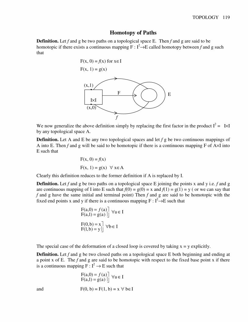
TOPOLOGY 119

f

F E

(x,0)

Homotopy of Paths Definition. Let f and g be two paths on a topological space E. Then f and g are said to be homotopic if there exists a continuous mapping F : I2→E called homotopy between f and g such that

F(x, 0) = f(x) for x∈I

F(x, 1) = g(x)

(x,1)

We now generalize the above definition simply by replacing the first factor in the product I2 = I×I by any topological space A.

Definition. Let A and E be any two topological spaces and let f g be two continuous mappings of A into E. Then f and g will be said to be homotopic if there is a continuous mapping F of A×I into E such that

F(x, 0) = f(x)

F(x, 1) = g(x) ∀ x∈A

Clearly this definition reduces to the former definition if A is replaced by I.

Definition. Let f and g be two paths on a topological space E joining the points x and y i.e. f and g are continuous mapping of I into E such that f(0) = g(0) = x and f(1) = g(1) = y ( or we can say that f and g have the same initial and terminal point) Then f and g are said to be homotopic with the fixed end points x and y if there is a continuous mapping F : I2→E such that

Ia)a(g)1,a(F)a()0,a(F ∈∀

== f

Iby)b,1(Fx)b,0(F ∈∀

==

The special case of the deformation of a closed loop is covered by taking x = y explicitly.

Definition. Let f and g be two closed paths on a topological space E both beginning and ending at a point x of E. The f and g are said to be homotopic with respect to the fixed base point x if there is a continuous mapping F : I2 → E such that

Ia)a(g)1,a(F)a()0,a(F ∈∀

== f

and F(0, b) = F(1, b) = x ∀ b∈I

I×I

THE FUNDAMENTAL GROUP AND COVERING SPACES

120

Definition. A closed path f on a topological space E beginning and ending at x will be said to be shrinkable to x or to be homotopic to a constant w.r.t to the base point x if f is homotopic to the mapping e : I→E defined by e(a) = x for all a∈I with respect to the base point x.

Thus shrinking a path f to be point x amounts to constructing a continuous mapping F of I2 into E whose restriction to the lower side (b= 0) gives the path f, while the other three sides are carried into x.

Definition. A topological space E will be said to be simply connected w.r. to the base point x if every closed path in E beginning and ending at x is shrinkable to x.

Theorem 1. The relation of homotopy w.r.t to x of paths based on x is an equivalence relation on the set of all paths in E based on x.

Proof. We must show that (i) f ∼ f for every path f based on x (reflexivity) (ii) f ∼ f implies g ∼ f for every pair of paths based on x (symmetry) (iii) If f, g, h are paths based on x such that f ∼ g and g ∼ h, then f ∼ h (transitivity).

(i) To prove that f ∼ f, define the mapping F : I2→E by setting F(s, t) = f(s). Then F is clearly a continuous mapping of I2 into E. Setting t = 0 and t = 1, we obtain F(s, 0) = f(s) F(s, 1) = f(s) and setting s = 0 and s = 1, we obtain F(0, t) = f(0) = x (initial point) F(1, t) = f(1) = x (Final point) Hence f ∼ f. (ii) Let f and g be given such that f ∼ g. Then there is a continuous mapping F : I2−E such that F(s, 0) = f(s), F(s, 1) = g(s) F(0, t) = F′(1, t) = x. We define the mapping

F* : I2→E by setting F*(s, t) = F(s, 1−t)

F*(s, 0) = F(s, 1) = g(s) F*(s, 1) = F(s, 0) = f(s) F*(0, t) = F(0, 1−t) = x F*(1, t) = F(1, 1−t) = x which proves that g ∼ f .

(iii) Let f, g, h be given such that f ∼ g and g ∼ h. Therefore there exists continuous mapping F′ and F′′ of I2 into E satisfying the following : F′(s, 0) = f(s) (1) F′(s, 1) = g(s) for s∈I (2) F′′(s, 0) = g(s) (3) F′′(s, 1) = h(s) (4)

F′(0, t) = F′(1, t) = F′′(0, t) = F′′(1, t) = x for t∈I (5) Define F : I2→E such that

F(s, t) = F′(s, 2t) if 0 ≤ t ≤21

TOPOLOGY 121

F(s, t) = F′′(s, 2t−1) if 21

≤ t ≤ 1

The first thing to check is that F is infact properly defined as mapping, for both parts of its

definition apply when t = 21

and they might contradict one another. Such a contradiction does not

however arise for by (2) and (3),

F′(s, 1) = F′′(s, 0) = g(s) and so F

21

,s = g(s) by both parts of the

definition

The next thing to verify is that F is continuous. It is clear that if t ≠21

, F is continuous

which follows directly from the continuity of F′ or F′′ according as t <21

or t >21

. Suppose now

that U is a nbd in E of F

21

,s for some s∈I. Then the continuity of F′ implies that there is a

number ξ′ such that if |s1 − s| < ξ′ and |2t1 − | < 2ξ′, F′(s1, 2t1) will lie in the nbd U of F′(s, 1) =

F

21

,s . Similarly the continuity of F′′ implies that there is a number ξ′′ such that if |s1 −s| < ξ′′

and |(2t1−1) −0| < 2ξ′′ then F′′(s1, 2t1−1) will lie in the nbd U of F′′(s, 0) = F

21

,s . The

inequalities imposed on s1 and t1 in the last two statements are all satisfied if |s1−s| < ξ and 21

t1 −

<ξ, where ξ = min (ξ′, ξ′′). Thus these two statements combine to show that if |s1−s|<ξ and

21

t1 − <ξ, then F(s1, t1) ∈U. The continuity of F is thus proved for points at which t = 21

. F has

thus been shown to be a continuous mapping of I2 into E. It remains to show that it gives the required homotopy of f and h. For t = 0, F(s, 0) = F′(s, 0) = f(s) by (1) and for t = 1 F(s, 1) = F′′(s, 1) = h(s) by (4) Also F(0, t) = F′(0, 2t) = x by (5)

where 0 ≤ t ≤ 21

F(0, t) = F′′(0, 2t−1) when 21 ≤ t ≤ 1.

= x by (5) Similarly

F(1, t) = F′(1, 2t) if 0 ≤ t ≤ 21

= x by (5)

F(1, t) = F′′(1, 2t−1) if 21 ≤ t ≤ 1

= x by (5). and so all the verifications are complete and f ∼ h .

THE FUNDAMENTAL GROUP AND COVERING SPACES

122

Remark. Since homotopy w.r to a base point x is an equivalence relation, all the paths based on x are divided into equivalence classes.

Definition. The equivalence classes of paths based on x∈E corresponding to the relation of homotopy with respect to the base point x will be called homotopy classes of paths on E w.r. to the base point x.

Definition. Let f and g be two closed paths on a topological space E based on a point x. Then the symbol fg, called the product of f and g is the mapping of I into E such that

(fg) (s) = f(2s) for 0 ≤ s ≤ 21

(fg) (s) = g(2s−1) for 21

≤ s ≤ 1.

Remark :- We claim that f g so defined is a path.

In 0 ≤ s < 21

, f g is continuous because of continuity of f . In 21

< s ≤ 1, fg is continuous because

of continuity of g. So s = 21

is the only point which needs attention. Let s = 21

and let U be a nbd

in E of f(g)(s). Then due to the continuity of f at s =21

, there exists δ1 such that if

|2s′ − 2s| < 2δ1 i.e. |s′ −s| < δ1

|s −21

| < δ1

=21

s

then f(2s′) ∈U

Similarly due to the continuity of g at s =21

we have if

|2s′ −1 −(2s−1)| < 2δ2

i.e. |s′ −21

| <δ2 (putting s =21

)

then g(2s′−1) ∈U. let δ = min (δ1, δ2). Then if

|s′ −21

| < δ

then f(2s′) and g(2s′−1) both belong to U and therefore fg is continuous at 21

. Thus fg : I→E is a

continuous mapping. Moreover fg(0) = f(0) = x fg(1) = g(1) = x So the product of two paths based on x is again a path based on x.

We shall now show that the homotopy class of fg depends only on those of f and g.

Theorem 2. If f, f ′, g, g′ are paths in a topological space E based on a point x and if f ∼ f ′, g ∼ g′, then fg ∼ f ′ g′. Proof. Since f ∼ f′ and g ∼ g′, there are continuous mapping F and G of I2 into E such that F(s, 0) = f(s) (1) F(s, 1) = f ′(s) (2)

TOPOLOGY 123

G(s, 0) = g(s) (3) G(s, 1) = g′(s) (4)

F(0, t) = F(1, t) = G(0, t) = G(1, t) = x (5) Define H : I2 →E by setting

H(s, t) = F(2s, t), 0 ≤ s ≤21

H(s, t) = G(2s−1, t) 21

≤ s ≤ 1.

we observe that this definition is not self contradictory for s = 21

, because it follows from the first

part of the definition that

H(21

, t) = F(1, t) = x by (5)

and by the second part of the definition that

H(21

, t) = G(0, t) = x by (5)

Next the continuity of H must be shown. Only the points with s =21

require attention. Let U be a

nbd of H(21

, t) for some fixed t. Since F is continuous, there exists δ1> 0 such that if

|2s′ − 2s| < δ1 and | t′ − t| < δ1 i.e. if |s′ − s| < δ1 and |t′ −t| < δ1, then F(2s′, t′) ∈U Similarly G is continuous and so ∃ δ2 such that if |(2s′−1) − (2s−1)| < 2δ2 and |t′ − t| < δ2 i.e. if |s′ −s| < δ2 and |t′ −t| < δ2, then G(2s′ −1, t′) ∈U Let δ = min (δ1, δ2), then if

|s′−21

| < and |t′ −t| < δ

Then we have F(2s′, t′) ∈U and g(2s′ −1, t′) ∈U. Hence H(s, t) is continuous. Moreover

H(s, 0) = F(2s, 0) = f (2s), for 0 ≤ s ≤ 21

H(s, 0) = G(2s−1, 0) = g(2s−1) for 21

≤ s ≤ 1.

If this is compared with the definition of fg, we see that H(s, 0) = fg(s). Similarly

H(s, 1) = F(2s, 1) = f ′(2s), for 0 ≤ s ≤ 21

THE FUNDAMENTAL GROUP AND COVERING SPACES

124

H(s, 1) = G(2s−1, 1) = g′(2s−1) for 21

≤ s ≤ 1.

Comparing this with the definition of f ′ g′, we see that H(s, 1) = (f ′ g′) (s) Also H(0, t) = F(0, t) = x by (5) H(1, t) = G(1, t) = x

Thus all the necessary conditions on H have been verified and it has been proved as required that fg ∼ f ′ g′.

Definition. Let f and g be two homotopy classes of paths based on x w.r. to the base point x and let f be a path belonging to f, g a path belonging to g. The product f g of f and g is defined to be the homotopy class to which the path fg belongs.

By the above theorem, this defines a homotopy class depending on the classes f and g and not on the representatives f and g. For if f ′ and g′ are two more paths belonging to f and g respectively fg ∼ f ′g′ and so fg and f ′g′ belong to the same homotopy class.

Theorem 3. Let E be a topological space and x is a point of E. Then the homotopy classes w.r.t the base point x of paths based on x are the elements of a group having the product just defined as group operation

Proof. The proof of this theorem consists of three parts (i) to show that the product operator between homotopy classes is associative (ii) to prove the existence of an identity element (iii) to prove that each homotopy class has an inverse

(i) let f, g, h be three paths based on x and f, g,h their homotopy classes. We have to show that (f g)h = f(gh).

It is sufficient to show that

(fg)h ∼ f(gh) By definition, fg is a continuous mapping of I into E such that

(fg)(s) = f(2s) 0 ≤ s ≤ 21

(fg)(s) = g(2s−1) 21

≤ s ≤ 1.

Applying the definition again to the product of fg and h, it turns out that

((fg)h)(s) = fg(2s) 0 ≤ s ≤ 21

((fg)h)(s) = h(2s−1) 21

≤ s ≤ 1

Combining these statements, it follows that (fg)h is a continuous mapping of I into E such that

((fg)h)(s) = f(4s), 0 ≤ s ≤ 41

((fg)h)(s) = g(4s−1), 41 ≤ s ≤

21

(1)

((fg)h)(s) = h(2s−1), 21 ≤ s ≤ 1

Similarly f(gh) is a continuous mapping of I into E such that

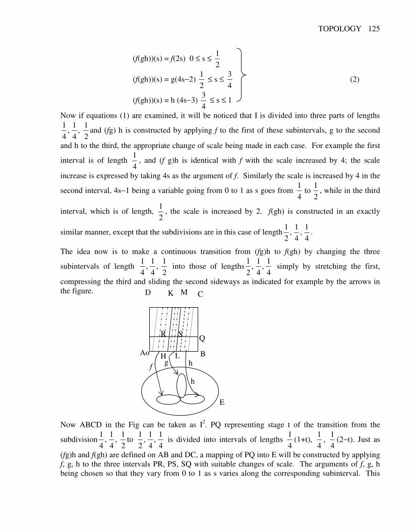
TOPOLOGY 125

E

f g hBAo H L

Q

C MK D

(f(gh))(s) = f(2s) 0 ≤ s ≤ 21

(f(gh))(s) = g(4s−2) 21

≤ s ≤ 43

(2)

(f(gh))(s) = h (4s−3) 43

≤ s ≤ 1

Now if equations (1) are examined, it will be noticed that I is divided into three parts of lengths

21

,41

,41

and (fg) h is constructed by applying f to the first of these subintervals, g to the second

and h to the third, the appropriate change of scale being made in each case. For example the first

interval is of length 41

, and (f g)h is identical with f with the scale increased by 4; the scale

increase is expressed by taking 4s as the argument of f. Similarly the scale is increased by 4 in the

second interval, 4s−1 being a variable going from 0 to 1 as s goes from 21

to41

, while in the third

interval, which is of length, 21

, the scale is increased by 2. f(gh) is constructed in an exactly

similar manner, except that the subdivisions are in this case of length41

,41

,21

.

The idea now is to make a continuous transition from (fg)h to f(gh) by changing the three

subintervals of length 21

,41

,41

into those of lengths41

,41

,21

simply by stretching the first,

compressing the third and sliding the second sideways as indicated for example by the arrows in the figure.

Now ABCD in the Fig can be taken as I2. PQ representing stage t of the transition from the

subdivision21

,41

,41

to 41

,41

,21

is divided into intervals of lengths 41

(1+t), 41

, 41

(2−t). Just as

(fg)h and f(gh) are defined on AB and DC, a mapping of PQ into E will be constructed by applying f, g, h to the three intervals PR, PS, SQ with suitable changes of scale. The arguments of f, g, h being chosen so that they vary from 0 to 1 as s varies along the corresponding subinterval. This

R S

h

THE FUNDAMENTAL GROUP AND COVERING SPACES

126

mapping which will be called F(s, t) will be equal to f

+ t1s4

on PR, to g(4s−t−1) on RS and to

h

−−−t2

2ts4on SQ. Thus we consider the function F : I×I→X defined by

F(s, t) =

≤≤+

−−−

+≤≤+−−

+≤≤

+

1s4

2tt2

)s1(41h

42t

s4

1t)1ts4(g

41t

s0t1

s4f

Then F is continuous. The continuity follows at once from the continuity of f, g and h. Also F(s, 0) = [(f g)h](s) F(s, 1) = [f(g h)](s) that is F coincides with (fg)h on the lower side of I2 and with f(gh) on the upper side. Moreover F(0, t) = F(1, t) = x for all t. Hence F is the required homotopy of (fg)h and f(gh). (ii) We shall use the symbol e to denote a constant mapping of I into E defined by e(s) = x ∀ s∈I.

The second part of the theorem will be proved by showing that the homotopy class e of the constant mapping e acts as identity. That is to say it will be shown that for any path f based on x, ef ∼ f e ∼ f By definition

(ef) (s) = e(2s), 0 ≤ s ≤ 21

= f(2s−1), 21

≤ s ≤ 1.

that is

(ef)s = e(2s) = x 0 ≤ s ≤ 21

= f(2s−1), 21

≤ s ≤ 1.

Thus I is divided in half, the first half being mapped on x, while f is applied to the second half with the scale doubled.

The idea now is to shrink steadily the part mapped on x while extending the part to which f is mapped. In the Fig below, ABCD is I2, AB s bisected at P and PD is joined. The horizontal line

QR at height t is divided into intervals of lengths 21

(1−t) at 21

(1+t), and as t varies from 0 to 1, it

is clear that these lengths change continuously from 21

, 21

(i.e. t = 0 in21

(1−t) and 21

(1+t)) to 0,

1(t = 1 in

+−2

t1and

2t1

)

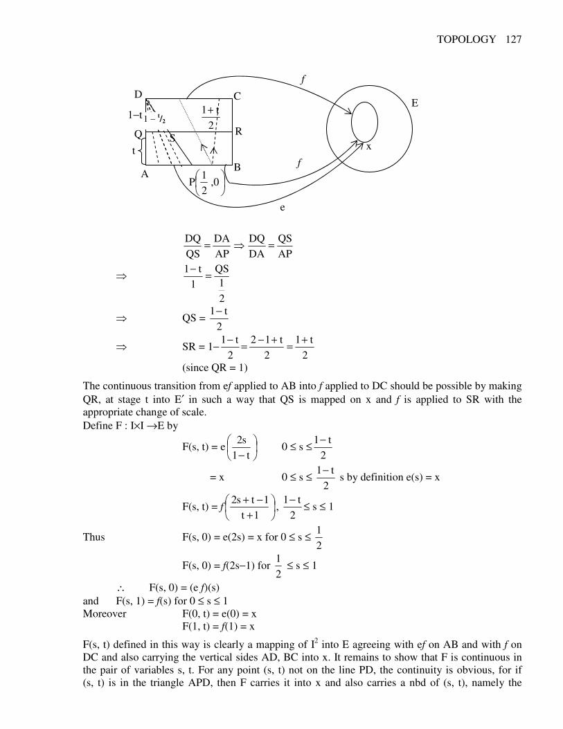
TOPOLOGY 127

f

E C

R

B f

e

0,21

P A

Q

t

1−t

D

APQS

DADQ

APDA

QSDQ ==

21

QS1

t1 =−

QS = 2

t1−

SR = 1−2

t12

t122

t1 +=+−=−

(since QR = 1)

The continuous transition from ef applied to AB into f applied to DC should be possible by making QR, at stage t into E′ in such a way that QS is mapped on x and f is applied to SR with the appropriate change of scale. Define F : I×I →E by

F(s, t) = e

− t1s2

0 ≤ s ≤2

t1−

= x 0 ≤ s ≤ 2

t1− s by definition e(s) = x

F(s, t) = f

+−+

1t1ts2

, 2

t1− ≤ s ≤ 1

Thus F(s, 0) = e(2s) = x for 0 ≤ s ≤ 21

F(s, 0) = f(2s−1) for 21

≤ s ≤ 1

∴ F(s, 0) = (e f)(s) and F(s, 1) = f(s) for 0 ≤ s ≤ 1 Moreover F(0, t) = e(0) = x F(1, t) = f(1) = x

F(s, t) defined in this way is clearly a mapping of I2 into E agreeing with ef on AB and with f on DC and also carrying the vertical sides AD, BC into x. It remains to show that F is continuous in the pair of variables s, t. For any point (s, t) not on the line PD, the continuity is obvious, for if (s, t) is in the triangle APD, then F carries it into x and also carries a nbd of (s, t), namely the

2

t1+

S

x

1 − t/2

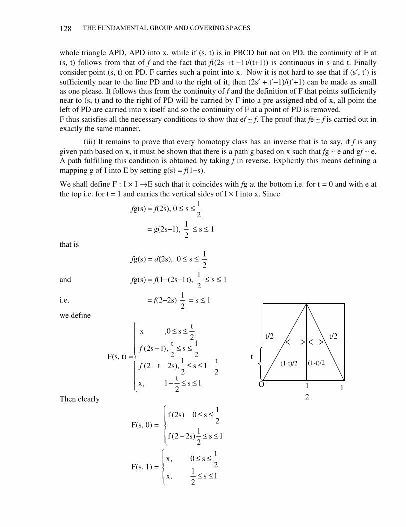
THE FUNDAMENTAL GROUP AND COVERING SPACES

128

O

21

1

whole triangle APD, APD into x, while if (s, t) is in PBCD but not on PD, the continuity of F at (s, t) follows from that of f and the fact that f((2s +t −1)/(t+1)) is continuous in s and t. Finally consider point (s, t) on PD. F carries such a point into x. Now it is not hard to see that if (s′, t′) is sufficiently near to the line PD and to the right of it, then (2s′ + t′−1)/(t′+1) can be made as small as one please. It follows thus from the continuity of f and the definition of F that points sufficiently near to (s, t) and to the right of PD will be carried by F into a pre assigned nbd of x, all point the left of PD are carried into x itself and so the continuity of F at a point of PD is removed. F thus satisfies all the necessary conditions to show that ef ∼ f. The proof that fe ∼ f is carried out in exactly the same manner.

(iii) It remains to prove that every homotopy class has an inverse that is to say, if f is any given path based on x, it must be shown that there is a path g based on x such that fg ∼ e and gf ∼ e. A path fulfilling this condition is obtained by taking f in reverse. Explicitly this means defining a mapping g of I into E by setting g(s) = f(1−s).

We shall define F : I × I →E such that it coincides with fg at the bottom i.e. for t = 0 and with e at the top i.e. for t = 1 and carries the vertical sides of I × I into x. Since

fg(s) = f(2s), 0 ≤ s ≤21

= g(2s−1), 21

≤ s ≤ 1

that is

fg(s) = d(2s), 0 ≤ s ≤ 21

and fg(s) = f(1−(2s−1)), 21

≤ s ≤ 1

i.e. = f(2−2s) 21

= s ≤ 1

we define

F(s, t) =

≤≤−

−≤≤−−

≤≤−

≤≤

1s2t

1,x2t

1s21

),s2t2(21

s2t

,)1s2(2t

s0,x

f

f t

Then clearly

F(s, 0) =

≤≤−

≤≤

1s21

)s22(f

21

s0)s2(f

F(s, 1) =

≤≤

≤≤

1s21

,x21

s0,x

t/2 t/2

2

t1−

2t1−

(1-t)/2

(1-t)/2

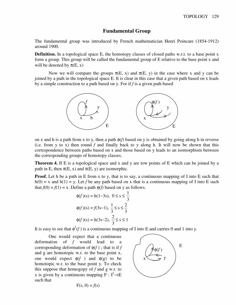
TOPOLOGY 129

E E

φ(f )

y x

Fundamental Group

The fundamental group was introduced by French mathematician Henri Poincare (1854-1912) around 1900.

Definition. In a topological space E, the homotopy classes of closed paths w.r.t. to a base point x form a group. This group will be called the fundamental group of E relative to the base point x and will be denoted by π(E, x)

Now we will compare the groups π(E, x) and π(E, y) in the case where x and y can be joined by a path in the topological space E. It is clear in this case that a given path based on x leads by a simple construction to a path based on y. For if f is a given path based

on x and h is a path from x to y, then a path φ(f) based on y is obtained by going along h in reverse (i.e. from y to x) then round f and finally back to y along h. It will now be shown that this correspondence between paths based on x and those based on y leads to an isomorphism between the corresponding groups of homotopy classes.

Theorem 4. If E is a topological space and x and y are tow points of E which can be joined by a path in E, then π(E, x) and π(E, y) are isomorphic.

Proof. Let h be a path in E from x to y, that is to say, a continuous mapping of I into E such that h(0) = x and h(1) = y. Let f be any path based on x that is a continuous mapping of I into E such that f(0) = f(1) = x. Define a path φ(f) based on y as follows.

φ(f )(s) = h(1−3s), 0 ≤ s ≤ 31

φ(f )(s) = f(3s−1), 32

s31 ≤≤

φ(f )(s) = h(3s−2), 32 ≤ s ≤ 1

It is easy to see that φ3(f ) is a continuous mapping of I into E and carries 0 and 1 into y.

One would expect that a continuous deformation of f would lead to a corresponding deformation of φ(f ) ; that is if f and g are homotopic w.r. to the base point x, one would expect φ(f ) and φ(g) to be homotopic w.r. to the base point y. To check this suppose that homogopy of f and g w.r. to x is given by a continuous mapping F : I2→E such that F(s, 0) = f(s)

f y x h

φ(f ) y x

E

THE FUNDAMENTAL GROUP AND COVERING SPACES

130

F(s, 1) = g(s) F(0, t) = F(1, t) = x ∀ s, t Define G by setting

G(S, t) =

≤≤−

∀≤≤−

∀≤≤−

talland1s32

),2s3(h

tand32

s31

),t,1s3(F

tand31

s0),s31(h

It can be shown that G is a continuous mapping of I2 into E. Moreover we observe

G(s, 0) =

≤≤−

≤≤−=−

≤≤−

1s32

),2s3(h32

s31

),1s3()0,1s3(F

talland31

s0),s31(h

f

G(s, 1) =

≤≤−

≤≤−=−

≤≤−

1s32

),2s3(h32

s31

),1s3(g)1,1s3(F31

s0),s31(h

G(0, t) = h(1) = y G(1, t) = h(1) = y

Therefore G is a homotopy between φ(f ) and φ(g). It follows therefore that all paths in a given homotopy class w.r.t the base point x are mapped by φ into the same homotopy class w.r.t y. If f is a homotopy class w.r.t x and f is a path in this class then the homotopy class w.r.t y of φ(f ) will be denoted by Φ(f ). Φ is thus a well defined mapping of π (E, x) into π(E, y)

In exactly the same way a mapping ψ of π(E, y) into π(E, x) can be constructed. To do this let g be a given path based on y and define ψ(g) as a path based on x, the definition being similar to that of φ(f ) above.

ψ(g)(s) =

≤≤−

≤≤−

≤≤

1s32

),s33(g32

s31

),1s3(g31

s0),s3(h

Having done this ψ is defined as the mapping of π(E, y) into π(E, x) which maps the homotopy class of g on that of ψ(g).

Now we will show that the mapping Φ andψ are inverse to one another, this will show that both mappings are one-one and onto. In order to do this it will be sufficient to prove that if f is a given path based on x, then ψ(φ(f )) is homotopic to f with respect to the base point x and that if g is a path based on y then φ(ψ(g)) is homotopic to g with respect to the base point y. The full definition of ψ(φ(f )) is as follows:

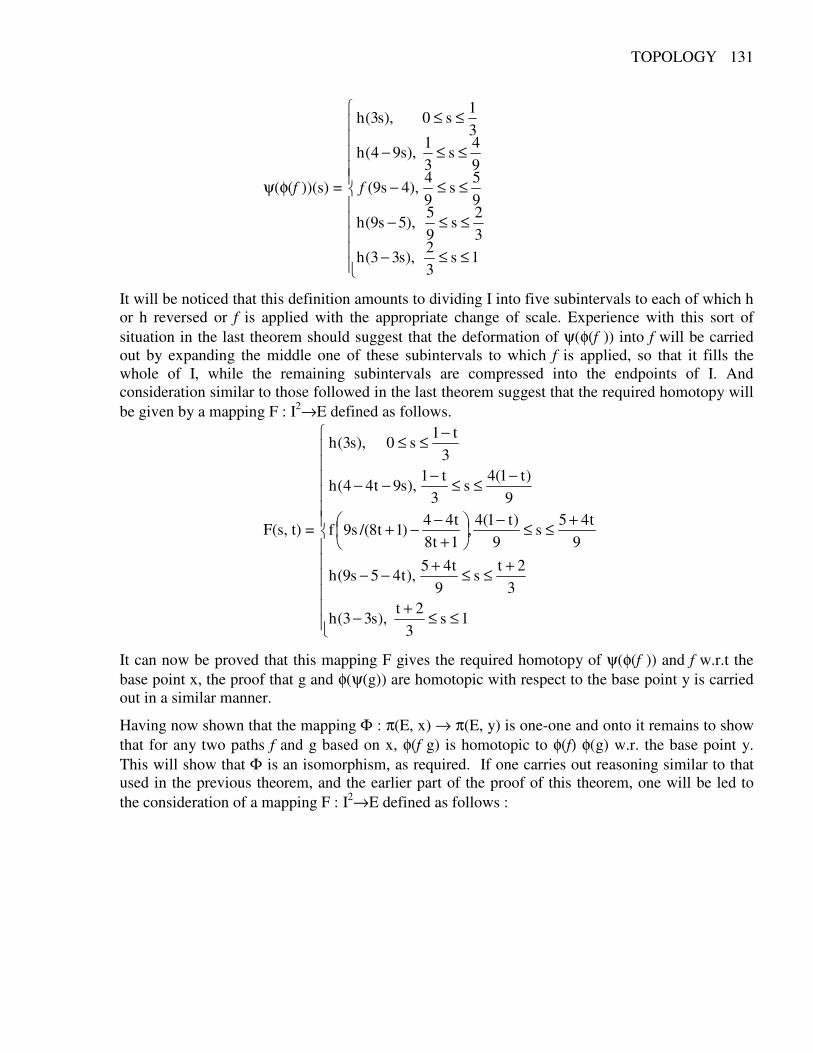
TOPOLOGY 131

ψ(φ(f ))(s) =

≤≤−

≤≤−

≤≤−

≤≤−

≤≤

1s32

),s33(h32

s95

),5s9(h95

s94

),4s9(94

s31

),s94(h31

s0),s3(h

f

It will be noticed that this definition amounts to dividing I into five subintervals to each of which h or h reversed or f is applied with the appropriate change of scale. Experience with this sort of situation in the last theorem should suggest that the deformation of ψ(φ(f )) into f will be carried out by expanding the middle one of these subintervals to which f is applied, so that it fills the whole of I, while the remaining subintervals are compressed into the endpoints of I. And consideration similar to those followed in the last theorem suggest that the required homotopy will be given by a mapping F : I2→E defined as follows.

F(s, t) =

≤≤+−

+≤≤+−−

+≤≤−

+−−+

−≤≤−−−

−≤≤

1s3

2t),s33(h

32t

s9

t45),t45s9(h

9t45

s9

)t1(4,

1t8t44

)1t8/(s9f

9)t1(4

s3

t1),s9t44(h

3t1

s0),s3(h

It can now be proved that this mapping F gives the required homotopy of ψ(φ(f )) and f w.r.t the base point x, the proof that g and φ(ψ(g)) are homotopic with respect to the base point y is carried out in a similar manner.

Having now shown that the mapping Φ : π(E, x) → π(E, y) is one-one and onto it remains to show that for any two paths f and g based on x, φ(f g) is homotopic to φ(f) φ(g) w.r. the base point y. This will show that Φ is an isomorphism, as required. If one carries out reasoning similar to that used in the previous theorem, and the earlier part of the proof of this theorem, one will be led to the consideration of a mapping F : I2→E defined as follows :

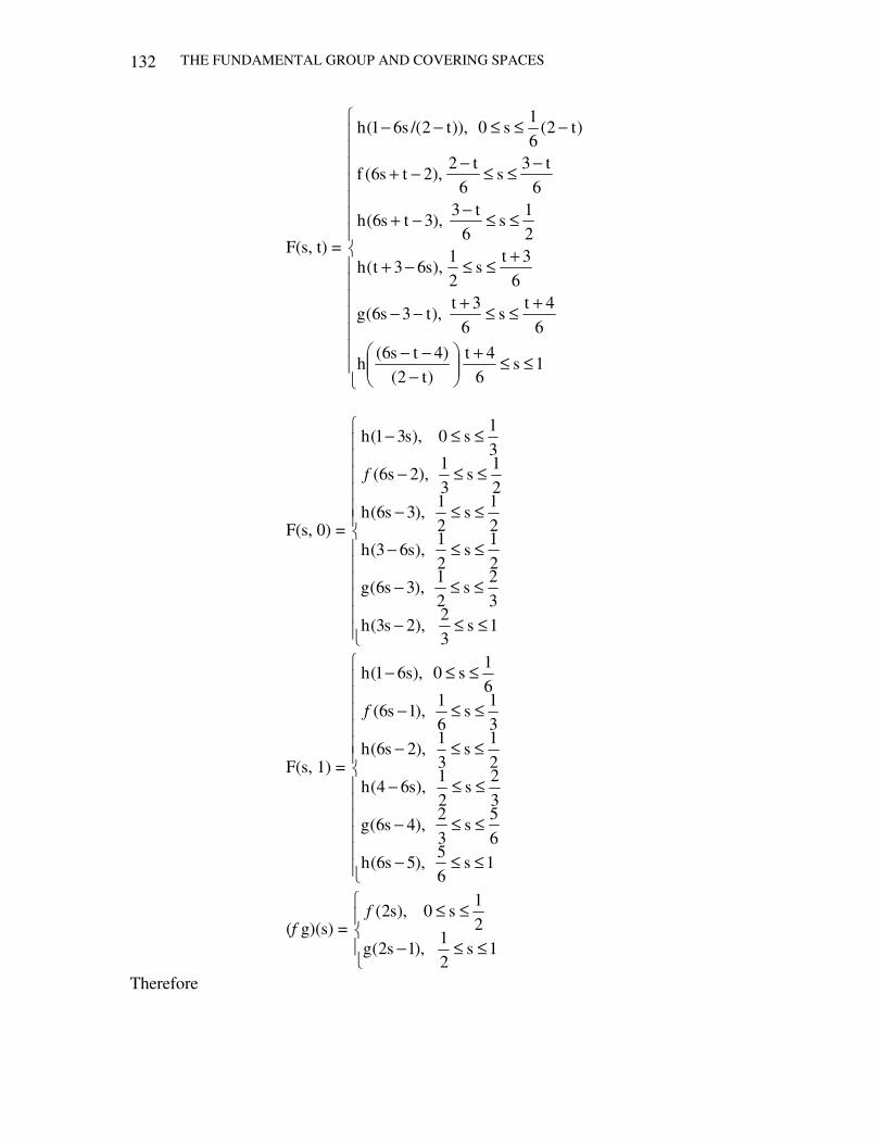
THE FUNDAMENTAL GROUP AND COVERING SPACES

132

F(s, t) =

≤≤+

−−−

+≤≤+−−

+≤≤−+

≤≤−−+

−≤≤−−+

−≤≤−−

1s6

4t)t2(

)4ts6(h

64t

s6

3t),t3s6(g

63t

s21

),s63t(h

21

s6

t3),3ts6(h

6t3

s6

t2),2ts6(f

)t2(61

s0)),t2/(s61(h

F(s, 0) =

≤≤−

≤≤−

≤≤−

≤≤−

≤≤−

≤≤−

1s32

),2s3(h32

s21

),3s6(g21

s21

),s63(h21

s21

),3s6(h21

s31

),2s6(31

s0),s31(h

f

F(s, 1) =

≤≤−

≤≤−

≤≤−

≤≤−

≤≤−

≤≤−

1s65

),5s6(h65

s32

),4s6(g32

s21

),s64(h21

s31

),2s6(h31

s61

),1s6(61

s0),s61(h

f

(f g)(s) =

≤≤−

≤≤

1s21

),1s2(g21

s0),s2(f

Therefore

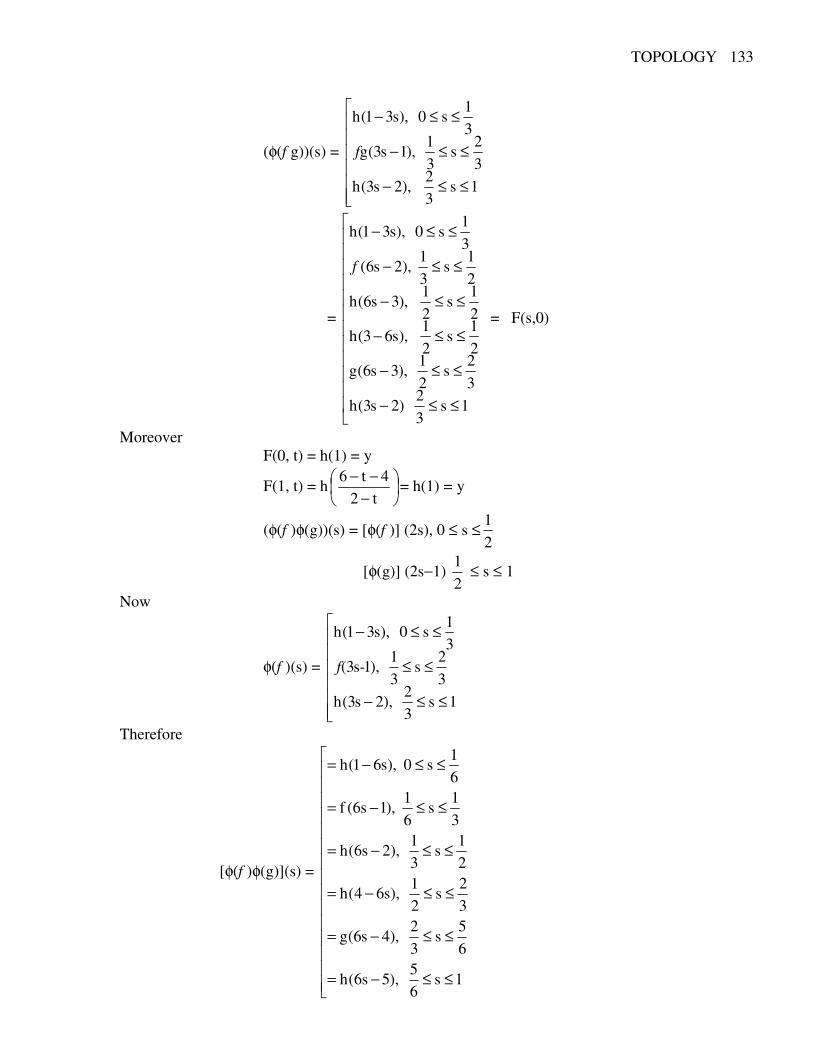
TOPOLOGY 133

(φ(f g))(s) =

≤≤−

≤≤−

≤≤−

1s32

),2s3(h32

s31

),1s3(g31

s0),s31(h

f

=

≤≤−

≤≤−

≤≤−

≤≤−

≤≤−

≤≤−

1s32

)2s3(h32

s21

),3s6(g21

s21

),s63(h21

s21

),3s6(h21

s31

),2s6(31

s0),s31(h

f

= F(s,0)

Moreover F(0, t) = h(1) = y

F(1, t) = h

−−−t2

4t6= h(1) = y

(φ(f )φ(g))(s) = [φ(f )] (2s), 0 ≤ s ≤21

[φ(g)] (2s−1) 21

≤ s ≤ 1

Now

φ(f )(s) =

≤≤−

≤≤

≤≤−

1s32

),2s3(h32

s31

),1s-3(31

s0),s31(h

f

Therefore

[φ(f )φ(g)](s) =

≤≤−=

≤≤−=

≤≤−=

≤≤−=

≤≤−=

≤≤−=

1s65

),5s6(h

65

s32

),4s6(g

32

s21

),s64(h

21

s31

),2s6(h

31

s61

),1s6(f

61

s0),s61(h

THE FUNDAMENTAL GROUP AND COVERING SPACES

134

It can be now shown that F gives the required homotopy w.r.t base point y of φ(f g) and φ(f)φ(g). This completes the proof of the theorem.

Cor. If E is an arcwise connected space, the group π(E, x) is independent of the base point x.

Proof. In this case any pair of points x and y of E can be joined by a path in E, and so π(E, x) and π(E, y) are isomorphic for any x and y in E. Hence π(E, x) is the same as π(E, y) from the point of view of group theory.

Remark. It follows from what has been said that, if E is an arcwise connected space, one can speak without ambiguity of the fundamental group of E without mentioning any base point, the understanding being that this group is π(E, x) for any arbitrary x in E. The fundamental group of an arcwise connected space will be denoted by π(E).

Now it will be shown that the fundamental group of an arcwise connected space is topologically invariant. This means that if E and E′ are two homemorphic arcwise connected spaces then π(E) and π(E′) are isomorphic.

Theorem 5. Let E and E′ be homeomorphic arcwise connected spaces, then π(E) and π(E′) are isomorphic.

Proof. Let f be the homeomorphism of E onto E′ and let g be the inverse of f. If x∈E, then we write y = f(x). If h is any path in E based on x, then the mapping foh I→E′ is a path in E′ based on y, for foh(0) = f(h(0)) = f(x) = y foh(1) = f(h(1)) = f(x) = y [ f : E→E′, h : I→E h(0) = h(1) = x foh : I→E]

Suppose that k is a second path in E based on x and that h is homotopic to k, so there exists a continuous mapping F : I2→E such that

Is)s(k)1,s(F)s(h)0,s(F ∈

==

F(0, t) = F(1, t) = x, t∈I Then the mapping foF : I2→E′ is such that (foF) (s, 0) = f(F(s, 0)) = f(h(s)) = foh(s) (foF) (s, 1) = f(F(s, 1)) = f(k(s)) = fok(s) (foF)(0, t) = f(F(0, t)) = f(x) = y (foF) (1,t) = f(F(1, t)) = f(x) = y.

Thus whenever h and k based on x are homotopic, foh and fok based on y are homotopic this shows that if h is a given homotopy class on E w.r. the base point x, then for any representative path h ofh, foh always lies in the same homotopy class φ(h) on E′, w.r.t the point y. Thus we have constructed a mapping φ : π(E)→π(E′)

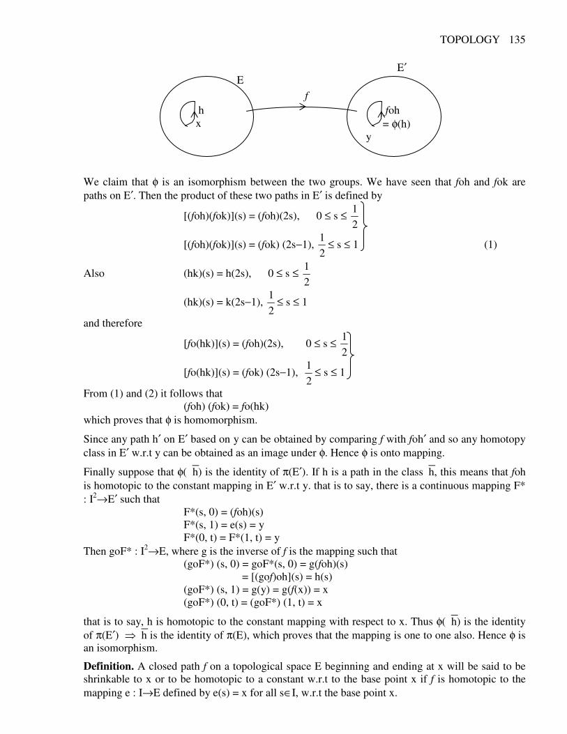
TOPOLOGY 135

f

E′ E

We claim that φ is an isomorphism between the two groups. We have seen that foh and fok are paths on E′. Then the product of these two paths in E′ is defined by

[(foh)(fok)](s) = (foh)(2s), 0 ≤ s ≤ 21

[(foh)(fok)](s) = (fok) (2s−1), 21 ≤ s ≤ 1 (1)

Also (hk)(s) = h(2s), 0 ≤ s ≤ 21

(hk)(s) = k(2s−1), 21 ≤ s ≤ 1

and therefore

[fo(hk)](s) = (foh)(2s), 0 ≤ s ≤ 21

[fo(hk)](s) = (fok) (2s−1), 21 ≤ s ≤ 1

From (1) and (2) it follows that (foh) (fok) = fo(hk) which proves that φ is homomorphism.

Since any path h′ on E′ based on y can be obtained by comparing f with foh′ and so any homotopy class in E′ w.r.t y can be obtained as an image under φ. Hence φ is onto mapping.

Finally suppose that φ(h) is the identity of π(E′). If h is a path in the classh, this means that foh is homotopic to the constant mapping in E′ w.r.t y. that is to say, there is a continuous mapping F* : I2→E′ such that F*(s, 0) = (foh)(s) F*(s, 1) = e(s) = y F*(0, t) = F*(1, t) = y Then goF* : I2→E, where g is the inverse of f is the mapping such that (goF*) (s, 0) = goF*(s, 0) = g(foh)(s) = [(gof)oh](s) = h(s) (goF*) (s, 1) = g(y) = g(f(x)) = x (goF*) (0, t) = (goF*) (1, t) = x

that is to say, h is homotopic to the constant mapping with respect to x. Thus φ(h) is the identity of π(E′) h is the identity of π(E), which proves that the mapping is one to one also. Hence φ is an isomorphism.

Definition. A closed path f on a topological space E beginning and ending at x will be said to be shrinkable to x or to be homotopic to a constant w.r.t to the base point x if f is homotopic to the mapping e : I→E defined by e(s) = x for all s∈I, w.r.t the base point x.

h x

foh = φ(h) y

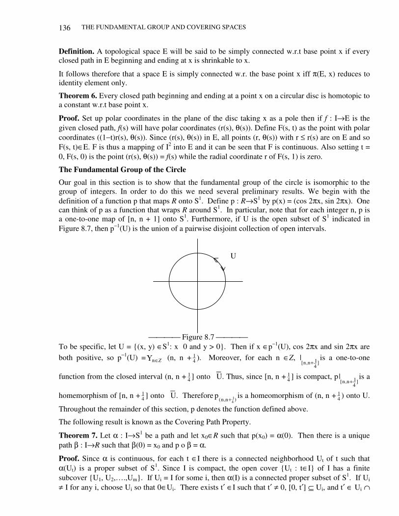
THE FUNDAMENTAL GROUP AND COVERING SPACES

136

Definition. A topological space E will be said to be simply connected w.r.t base point x if every closed path in E beginning and ending at x is shrinkable to x.

It follows therefore that a space E is simply connected w.r. the base point x iff π(E, x) reduces to identity element only.

Theorem 6. Every closed path beginning and ending at a point x on a circular disc is homotopic to a constant w.r.t base point x.

Proof. Set up polar coordinates in the plane of the disc taking x as a pole then if f : I→E is the given closed path, f(s) will have polar coordinates (r(s), θ(s)). Define F(s, t) as the point with polar coordinates ((1−t)r(s), θ(s)). Since (r(s), θ(s)) in E, all points (r, θ(s)) with r ≤ r(s) are on E and so F(s, t)∈E. F is thus a mapping of I2 into E and it can be seen that F is continuous. Also setting t = 0, F(s, 0) is the point (r(s), θ(s)) = f(s) while the radial coordinate r of F(s, 1) is zero.

The Fundamental Group of the Circle

Our goal in this section is to show that the fundamental group of the circle is isomorphic to the group of integers. In order to do this we need several preliminary results. We begin with the definition of a function p that maps R onto S1. Define p : R→S1 by p(x) = (cos 2πx, sin 2πx). One can think of p as a function that wraps R around S1. In particular, note that for each integer n, p is a one-to-one map of [n, n + 1] onto S1. Furthermore, if U is the open subset of S1 indicated in Figure 8.7, then p−1(U) is the union of a pairwise disjoint collection of open intervals. Figure 8.7 To be specific, let U = (x, y) ∈S1: x 0 and y > 0. Then if x ∈p−1(U), cos 2πx and sin 2πx are both positive, so p−1(U) = Υ Z∈n (n, n + 1

4 ). Moreover, for each n ∈Z, ]1

4n,n[

|+

is a one-to-one

function from the closed interval (n, n + 14 ] onto U. Thus, since [n, n + 1

4 ] is compact, p]1

4n,n[

|+

is a

homemorphism of [n, n + 14 ] onto U. Therefore

)n,n( 14

p + is a homeomorphism of (n, n + 14 ) onto U.

Throughout the remainder of this section, p denotes the function defined above.

The following result is known as the Covering Path Property.

Theorem 7. Let α : I→S1 be a path and let x0∈R such that p(x0) = α(0). Then there is a unique path β : I→R such that β(0) = x0 and p o β = α.

Proof. Since α is continuous, for each t ∈I there is a connected neighborhood Ut of t such that α(Ut) is a proper subset of S1. Since I is compact, the open cover Ut : t∈I of I has a finite subcover U1, U2,….,Um. If Ui = I for some i, then α(I) is a connected proper subset of S1. If Ui ≠ I for any i, choose Ui so that 0∈Ui. There exists t′ ∈I such that t′ ≠ 0, [0, t′] ⊆ Ui, and t′ ∈ Ui ∩

U

TOPOLOGY 137

Uj for some j ≠ i. If Ui ∪Uj = I, α([0, t′]) and α([t′, 1]) are connected proper subsets of S1. If Ui ∪ Uj ≠ I, choose t′′ ∈I such that t′′ > t′, [t′, t′′] ⊆ Uj and t′′ ∈ Uj ∩ Uk for some k (i ≠ k ≠ j). Since U1, U2,…,Um is a finite cover of I, after a finite number of steps, we will obtain t0, t1, t2,…, tn such that 0 = t0, tn = 1, ti−1 < ti and α([ti−1, ti]) is a connected proper subset of S1 for each i = 1, 2,…, n.

For each i = 0, 1, 2,…, n let Pi be the statement : There is a unique continuous function βi : [0, ti] →R such that βi(0) = x0 and poβi = α ]it,0[| . In order to prove the theorem, it is sufficient

to show that Pi is true for each i. It is clear that P0 is true. Suppose 0 < i ≤ n and Pi−1 is true. Let Vi−1 denote the component of p−1 (α[ti−1, ti])) that contains βi−1 (ti−1), and let pi−1 = p|Vi−1. Then pi−1 : Vi−1→α([ti−1, ti]) is a homemorphism. Define βi : [0, ti] →R by

βi(t) =

≤≤α≤≤β

−−

−

−−.tttif)),t(()p(

tt0if),t(i1i

11i

1i1i

Then βi is continuous, βi(0) = x0, and poβi = ]it,0[| . We must show that βi is unique. Suppose 'iβ :

[0, ti] →R is a continuous function such that 'iβ (0) = x0 and po '

iβ = ]it,0[| . If 0 ≤ t ≤ ti−1, then 'iβ (t) = βi(t) since Pi−1 is true. Suppose ti−1 < t ≤ ti. Since(po '

iβ ) (t) = α(t) ∈α([ti−1, ti]), 'iβ (t) ∈ p−1

(α([ti−1, ti])). Therefore 'iβ (t) ∈ Vi−1 since '

iβ is continuous and Vi−1 is a component of p−1(α([ti−1,

ti])). Therefore βi(t), 'iβ (t) ∈ Vi−1 and (pi−1 o βi)(t) = (pi−1 o '

iβ )(t). Hence βi(t) = 'iβ (t) since pi−1 is a

homeomorphism.

Example. Let α : I→S1 be a homemorphism that maps I onto 0yand0x:S)y,x( 1 >>∈ and has the property that α(0) = (1, 0) and α(1) = (0, 1), and let x0 = 2. Then the function β : I → R given by Theorem 6 is a homemorphism of I onto [2,2.25], which has the property that β(0) = 2 and β(1) = 2.25.

The following result is known as the Covering Homotopy Property.

Theorem 8. Let (X, T) be a topological space, let f : X→R be a continuous function, and let H : X × I→ S1 be a continuous function such that H(x, 0) =(p of)(x) for each x∈X. Then there is a continuous function F : X × I→R such that F(x, 0) = f(x) and (p oF) (x, t) = H(x, t) for each (x, t) ∈X × I.

Proof. For each x∈X, define αx : I→S1 by αx(t) = H(x, t). Now (p of )(x) = αx(0), and hence, by last Theorem (6) there is a unique path βx : I→R such that βx(0) = f(x) and poβx = αx. Define F : X × I →R by F(x, t) = βx(t). Then (poF)(x, t) = (poβx)(t) = H(x, t) and F(x, 0) = βx(0) = f(x).

We must show that F is continuous. Let x0∈X. For each t ∈I, there is a neighborhood Mt of x0 and a connected neighborhood Nt or t such that H(Mt × Nt) is contained in a proper connected subset of S1. Since I is compact, the open cover Nt : t∈I of I has a finite subcover N,...,N,N

nt2t1t. Let

m = Ι n1i itM= . Then M is a neighborhood of x0, and, for each i = 1,2,…m, H(M ×

itN ) is contained

a proper connected subset of S1. Thus there exist t0, t1, …, tm such that t0 = 0, tm = 1, and, for each j = 1, 2,…,m, tj−1 < tj and H(M ×[tj−1, tj]) is contained in a proper connected subset of S1.

For each j = 0, 1,…,m, let Pj be the statement : There is a unique continuous function Gj : M × [0, tj] →R such that Gj(x, 0) = f(x) and (p o Gj) (x, t) = H(x, t). We want to show that Pj is true for each j. It is clear that P0 is true. Suppose 0 < j ≤ m and Pj−1 is true. Let Uj−1 be a connected proper subset of S1 that contains H(M × Ij−1), let Vj−1 denote the component of p−1(Uj−1) that

THE FUNDAMENTAL GROUP AND COVERING SPACES

138

contains Gj−1(M × tj−1), and let pj−1 = p|vj−1. Then pj−1 : Vj−1 → Uj−1 is a homemorphism. Define Gj : M × [0, tj] → R by

Gj(x, t) =

≤≤≤≤

−−

−

−−

j1j1

1j

1j1j

tttif)),t,x(H()p(tt0if),t,x(G

Then Gj is continuous, Gj(x, 0) = f(x), and (p oGj) (x, t) = H(x, t). We must show that Gj is unique. Suppose '

jG : M × [0, tj] → R is a continuous function such that 'jG (x, 0) = f(x) and (p o '

jG )(x, t) =

H(x, t). If 0 ≤ t ≤ tj−1, then 'jG (x, t) = Gj(x, t) because Pj−1 is true. Suppose tj−1 < t ≤ tj. Since

(p o Gj)(x, t) = H(x, t)∈Uj−1, 'jG (x, t)∈ p−1 (Uj−1). Therefore, since '

jG is continuous and Vj−1 is a

component of p−1 (Uj−1), 'jG (x, t) ∈ Vj−1. Hence Gj(x, t) and '

jG (x, t) are members of Vj−1 and

(pj−1 oGj) (x, t) = (pj−1 o 'jG )(x, t). Thus, since pj−1 is a homemorphism, Gj(x, t) = '

jG (x, t). We have

proved that there is a unique continuous function G : M × I→R such that G(x, 0) = f(x) and (p o G)(x, t) = H(x, t). Therefore G = F|(M×I). Since M is a neighborhood of x0 in X, F is continuous at (x0, t) for each t ∈ I. Since x0 is an arbitrary member of X, F is continuous. This proof also shows that F is unique.

It α is a loop in S1 at (1, 0), then p(0) = α(0), and hence, by Theorem 6 there is a unique path β = I→R1 such that β(0) = 0 and poβ = α. Since (poβ)(1) = α(1) = (1, 0), β(1) ∈ p−1(1, 0), and hence β(1) is an integer. The integer β(1) is called the degree of the loop α, and we write deg(α) = β(1).

Example. Define α : I→S1 by α(x) = (cos 4πx, − sinπx). Then α “wraps” I around S1 twice in a clockwise direction. The unique path β : I → R such that β(0) = 0 and poβ = α given by Theorem 6 is defined by β(x) = −2x for each x∈I. Therefore deg(α) = β(1) = −2.

Theorem 9. Let α1 and α2 be loops in S1 at (1, 0) such that α1 ∼ p α2. Then deg(α1) = deg(α2).

Proof. Since α1 ∼ p α2, there is a continuous function H : I×I→S1 such that H(x, 0) = α1(x) and H(x, 1) = α2(x) for each x∈I and H(0, t) = H(1, t) = (1, 0) for each t∈I. By Theorem 6 there is a unique path β1 : I→R such that β1(0) = 0 and poβ1 = α1. Thus, by Theorem 8, there is a unique continuous function F : I × I→R such that (p oF)(x, t) = H(x, t) for each (x, t) ∈I×I and F(x, 0) = β1(x) for each x∈I. Define γ : I→R by γ(t) = F(0, t) for each t∈I. Then γ is continuous, and (p o γ)(t) = (p o F)(0, t) = H(0, t) = (1, 0) for each t∈I. Therefore γ(I) ⊆ p−1 (1, 0), and, since γ(I) is connected and p−1(1, 0) is a discrete subspace of R, γ is a constant function. Thus F(0, t) = γ(t) = γ(0) = F(0, 0) = β1(0) = 0 for each t∈I. Define β2 : I→R by β2(x) = F(x, 1) for each x∈I. Then β2(0) = F(0, 1) = 0 and (p o β2)(x) = (p o F) (x, 1) = H(x, 1) = α2(x) for each x∈I. By definition, deg(α1) = β1(1) and deg(α2) = β2(1). Now define a path δ : I→R by δ(t) = F(1, t) for each t∈I. Again (p o δ)(t) = (p o F)(1, t) = H(1, t) = (1, 0) for each t∈I, and hence δ(I) ⊆ p−1(1, 0). Therefore δ is a constant function, and hence F(1, t) = δ(t) = δ(0) = F(1, 0) = β1(0) = 0 for each t∈I. Therefore β2(1) = F(1, 1) = F(1, 0) = β1(1), and hence deg(α1) = deg(α2).

Remark :- Now we are ready to prove that the fundamental group of the circle is isomorphic to the group of integers. Since S1 is pathwise connected, the fundamental group of S1 is independent of the base point.

Theorem 10. π1 (S1, (1,0)) is isomorphic to the group of integers.

TOPOLOGY 139

Proof. Define φ : π1(S1, (1, 0)) → Z by φ([α]) = deg(α). By Theorem 9 φ is well-defined. Let [α1], [α2] ∈π1 (S1,(1, 0)). By Theorem 7 there are unique paths β1, β2, I→R such that β1(0) = β2(0) = 0, p o β1 = α1, and p o β2 = α2. By definition, deg(α1) = β1(1) and deg (α2) = β2(1). Define δ : I→R by

δ(x) =

≤≤−β+β≤≤β

.1xif),1x2()1(x0if),x2(

1221

121

Since β2(0) = 0, δ is continuous. Now δ(0) = β1(0) = 0, and, since p[(β1(1) + β2(2x−1)) = p(β2(2x−1)),

(p o δ)(x) =

≤≤−β≤≤β

1xif),1x2)(po(x0if),x2)(po(

122

121

=

≤≤−α≤≤α

1xif),1x2(x0if),x2(

122

121 = (α1∗ α2)(x).

Therefore φ([α1] o [α2]) = φ([α1 ∗ α2]) = deg(α1 ∗α2) = δ(1) = β1(1) + β2(1) = deg(α1) + deg(α2) = φ([α1]) + φ([α2]), and so φ is a homomorphism.

Now we show that φ maps π1 (S1, (1, 0)) onto Z. Let z ∈Z, and define a path α : I→R by α(t) = zt for each t ∈I. Then α(0) = 0 and α(1) = z, so poα : I→S1 is a loop in S1 at (1, 0). Therefore [p o α]∈π1 (S1, (1, 0)), and, by definition, deg(p o α) = α(1) = z. Thereforeφ([p o α]) = deg (p o α) = z.

Finally, we show that φ is one-to-one. Let [α1], [α2] ∈π1 (S1, (1, 0)) such that φ([α1]) = φ ([α2]). Then deg(α1) = deg(α2). By Theorem 7 there are unique paths β1, β2 : I→R such that β1(0) = β2(0) = 0, p o β1 = α1, and p o β2 = α2. By definition, deg (α1) = β1(1) and deg(α2) = β2(1). So β1(1) = β2(1). Define F : I × I → R by F(x, t) = (1−t) β1(x) + tβ2(x) for each (x, t) ∈ I × I. Then F(x, 0) = β1(x) and F(x, 1) = β2(x) for each x∈I and F(0, t) = 0 and F(1, t) = β1(1) = β2(1) for each t∈I. Therefore p o F : I × I→S1 is a continuous function such that (p o F)(x, 0) = (p o β1)(x) = α1(x) and (p o F)(x, 1) = (p o β2)(x) = α2(x) for each x∈I and (p o F)(0, t) = p(0) = (1, 0) and (p o F) (1, t) = (p o β1)(1) = α1(1) = (1, 0) for each t∈I. Thus α1 ∼ p α2, so [α1] = [α2]. Covering Spaces In this section we generalize Theorem 7 and 8 by replacing the function p:R→S1 defined by p(x) = (cos 2πx, sin 2πx) with a function called a “covering map” from an arbitrary topological space (E, T) into another topological space (B, u).

Definition. Let (E, T) and (B, u) be topological spaces, and let p : E→B be a continuous surjection. A n open subset U of B is evenly covered by p if p−1(U) can be written as the union of a pairwise disjoint collection Vα : α∈∧ of open sets such that for each α ∈∧, p|vα is a homemorphism of Vα onto U. Each Vα is called a slice of p−1(U).

Definition. Let (E, T) and B(, u) be topological spaces, and let p: E→B be a continuous surjection. If each member of B has a neighborhood that is evenly covered by p, then p is covering map and E is a covering space of B.

Note that the function p : R→S1 in Section 8.3 is covering map. Covering spaces were introduced by Poincare in 1883.

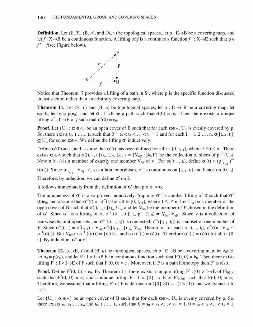
THE FUNDAMENTAL GROUP AND COVERING SPACES

140

E

p

B

f ′

X f

Definition. Let (E, T), (B, u), and (X, v) be topological spaces, let p : E→B be a covering map, and let f : X→B be a continuous function. A lifting of f is a continuous function f ′ : X→E such that p o f ′ = f(see Figure below).

Notice that Theorem 7 provides a lifting of a path in S1, where p is the specific function discussed in last section rather than an arbitrary covering map.

Theorem 11. Let (E, T) and (B, u) be topological spaces, let p : E → B be a covering map, let e0∈E, let b0 = p(e0), and let σ : I→B be a path such that σ(0) = b0. Then there exists a unique lifting σ′ : I →E of f such that σ′(0) = e0.

Proof. Let Uα : α ∈∧ be an open cover of B such that for each α∈∧, Uα is evenly covered by p. So, there exists t0, t1,…., tn such that 0 = t0 < t1 < … < tn = 1 and for each i = 1, 2,…, n, σ([ti−1, ti]) ⊆ Uα for some α∈∧. We define the lifting σ′ inductively.

Define σ′(0) = e0, and assume that σ′(t) has been defined for all t ∈[0, ti−1], where 1 ≤ i ≤ n. There exists α ∈∧ such that σ([ti−1, ti]) ⊆ Uα. Let v = Vαβ : β∈Γ be the collection of slices of p−1 (Uα). Now σ′(ti−1) is a member of exactly one member Vαγ of v . For t∈[ti−1, ti], define σ′(t) = (p αγv| )−1

(σ(t)). Since p αγv| : Vαγ→Uα is a homemorphism, σ′ is continuous on [ti−1, ti] and hence on [0, ti].

Therefore, by induction, we can define σ′ on I.

It follows immediately from the definition of σ′ that p o σ′ = σ.

The uniqueness of σ′ is also proved inductively. Suppose σ′′ is another lifting of σ such that σ′′ (0)e0, and assume that σ′′(t) = σ′′(t) for all t∈[0, ti−1], where 1 ≤ i≤ n. Let Uα be a member of the open cover of B such that σ([ti−1, ti]) ⊆ Uα, and let Vαγ be the member of V chosen in the definition of σ′. Since σ′′ is a lifting of σ, σ′′ ([ti−1, ti]) ⊆ p−1 (Uα) = Υ V∈ . Since V is a collection of

pairwise disjoint open sets and σ′′ ([ti−1, ti]) is connected, σ′′([ti−1, ti]) is a subset of one member of V. Since σ′′(ti−1) = σ′(ti−1) ∈Vαγ σ′′([ti−1, ti]) ⊆ Vαγ. Therefore, for each t∈[ti−1, ti], σ′′(t)∈ Vαγ ∩ p−1(σ(t)). But Vαγ ∩ p−1 (σ(t)) = σ′(t), and so σ′′(t) = σ′(t). Therefore σ′′(t) = σ′(t) for all t∈[0, ti]. By induction, σ′′ = σ′.

Theorem 12. Let (E, T) and (B, u) be topological spaces, let p : E→B be a covering map, let e0∈E, let b0 = p(e0), and let F : I × I→B be a continuous function such that F(0, 0) = b0. Then there exists lifting F′ : I × I→E of F such that F′(0, 0) = e0. Moreover, if F is a path homotopy then F′ is also.

Proof. Define F′(0, 0) = e0. By Theorem 11, there exists a unique lifting F′ :0 × I→E of F|0×I such that F′(0, 0) = e0 and a unique lifting F : I × 0 → E of F|I×0 such that F(0, 0) = e0. Therefore, we assume that a lifting F′ of F is defined on (0 ×I) ∪ (I ×0) and we extend it to I × I.

Let Uα : α ∈∧ be an open cover of B such that for each α∈∧, Uα is evenly covered by p. So, there exists s0, s1,…, sm and t0, t1,…., tn such that 0 = s0 < s1 <…< sm = 1, 0 = t0 < t1 <…< tn = 1,

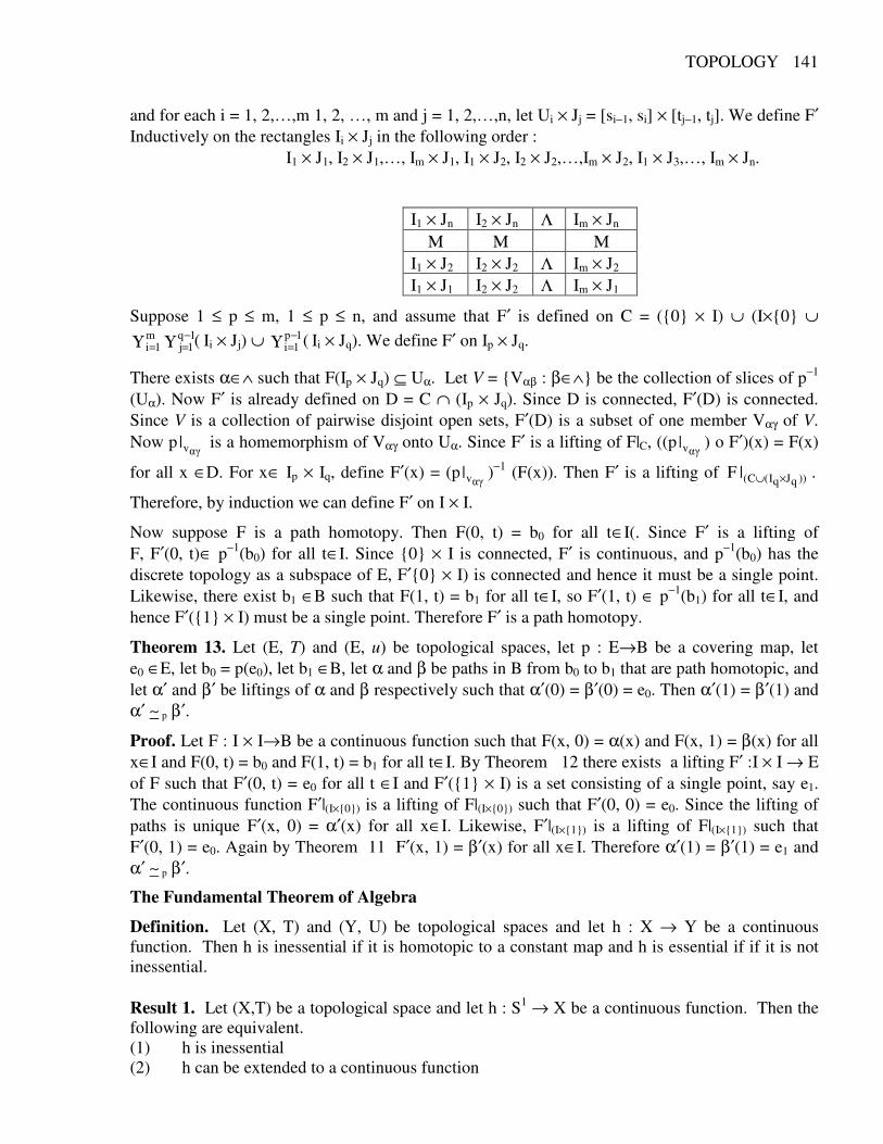
TOPOLOGY 141

and for each i = 1, 2,…,m 1, 2, …, m and j = 1, 2,…,n, let Ui × Jj = [si−1, si] × [tj−1, tj]. We define F′ Inductively on the rectangles Ii × Jj in the following order : I1 × J1, I2 × J1,…, Im × J1, I1 × J2, I2 × J2,…,Im × J2, I1 × J3,…, Im × Jn.

I1 × Jn I2 × Jn Λ Im × Jn Μ Μ Μ

I1 × J2 I2 × J2 Λ Im × J2 I1 × J1 I2 × J2 Λ Im × J1

Suppose 1 ≤ p ≤ m, 1 ≤ p ≤ n, and assume that F′ is defined on C = (0 × I) ∪ (I×0 ∪ Υ Υm

1i1q1j (=

−= Ii × Jj) ∪ Υ 1p

1i (−= Ii × Jq). We define F′ on Ip × Jq.

There exists α∈∧ such that F(Ip × Jq) ⊆ Uα. Let V = Vαβ : β∈∧ be the collection of slices of p−1 (Uα). Now F′ is already defined on D = C ∩ (Ip × Jq). Since D is connected, F′(D) is connected. Since V is a collection of pairwise disjoint open sets, F′(D) is a subset of one member Vαγ of V. Now p

v| is a homemorphism of Vαγ onto Uα. Since F′ is a lifting of F|C, ((pv| ) o F′)(x) = F(x)

for all x ∈D. For x∈ Ip × Iq, define F′(x) = (pv| )−1 (F(x)). Then F′ is a lifting of .|F ))qJqI(C( ×∪

Therefore, by induction we can define F′ on I × I.

Now suppose F is a path homotopy. Then F(0, t) = b0 for all t∈I(. Since F′ is a lifting of F, F′(0, t)∈ p−1(b0) for all t∈I. Since 0 × I is connected, F′ is continuous, and p−1(b0) has the discrete topology as a subspace of E, F′0 × I) is connected and hence it must be a single point. Likewise, there exist b1 ∈B such that F(1, t) = b1 for all t∈I, so F′(1, t) ∈ p−1(b1) for all t∈I, and hence F′(1 × I) must be a single point. Therefore F′ is a path homotopy.

Theorem 13. Let (E, T) and (E, u) be topological spaces, let p : E→B be a covering map, let e0 ∈E, let b0 = p(e0), let b1 ∈B, let α and β be paths in B from b0 to b1 that are path homotopic, and let α′ and β′ be liftings of α and β respectively such that α′(0) = β′(0) = e0. Then α′(1) = β′(1) and α′ ∼ p β′.

Proof. Let F : I × I→B be a continuous function such that F(x, 0) = α(x) and F(x, 1) = β(x) for all x∈I and F(0, t) = b0 and F(1, t) = b1 for all t∈I. By Theorem 12 there exists a lifting F′ :I × I → E of F such that F′(0, t) = e0 for all t ∈I and F′(1 × I) is a set consisting of a single point, say e1. The continuous function F′|(I×0) is a lifting of F|(I×0) such that F′(0, 0) = e0. Since the lifting of paths is unique F′(x, 0) = α′(x) for all x∈I. Likewise, F′|(I×1) is a lifting of F|(I×1) such that F′(0, 1) = e0. Again by Theorem 11 F′(x, 1) = β′(x) for all x∈I. Therefore α′(1) = β′(1) = e1 and α′ ∼ p β′.

The Fundamental Theorem of Algebra

Definition. Let (X, T) and (Y, U) be topological spaces and let h : X → Y be a continuous function. Then h is inessential if it is homotopic to a constant map and h is essential if if it is not inessential. Result 1. Let (X,T) be a topological space and let h : S1 → X be a continuous function. Then the following are equivalent. (1) h is inessential (2) h can be extended to a continuous function

THE FUNDAMENTAL GROUP AND COVERING SPACES

142

Result 2. Let (Y, U) be a topological space and let h : S1 → Y be an inessential function. Then h* is the zero homomorphism. The Fundamental Theorem of Algebra says that if n ∈N, then every polynomial equation of degree n with complex coefficients has at least one solution in the set of complex numbers. This theorem is difficult to prove, and most proofs involve non-algebraic concepts. We give a proof that uses the concepts used in the last sections.

Theorem 14. Let n ∈N and let xn + an−1 xn−1 +…+ a1x + a0 = 0 be a polynomial equation of degree n with complex coefficients. Then this equation has at least one solution in the set of complex numbers.

Proof. We consider the members of S1 to be complex numbers and define continuous function f : S1 → S1 by f(z) = zn. Let s0 = (1, 0) and consider the induced homomorphism f∗ : π1(S1, s0) → π1(S1, s0). Define σ : I → S1 by σ(x) = (cos 2πx, sin 2πx) = e2πix. Then f∗([σ]) = [f o σ] ∈π1 (S1, (1, 0)). Since (f o σ)(0) = (1, 0), the unique path α : I→R given by Theorem 7, is the path defined by g(x) = nx. Let p : R → S1 be the standard covering map defined by p(x) = (cos 2πx, sin 2πx). Then p o α = f o σ, so deg (f o σ) = n. From the proof that π1(S1, (1, 0)) is isomorphic to the group of integers (Theorem 10), we see that [f o σ] is not the identity element of π1 (S1, (1, 0)). Therefore f∗ is not the zero homomorphism.

First we show that we may assume that |an−1| + |an−2| +…+ |a0| < 1. We let c be a positive real number and substitute x = cy in the given polynomial equation to obtain the equation

(cy)n + an−1(cy)n−1 +…+ a1(cy) + a0 = 0 or yn + (an−1/c)yn−1 +…+ (a1/cn−1)y + a0/cn = 0.

Now choose c large enough so that |an−1/c| + |an−2/c2| +…+ |a1/cn−1| + |a0/cn| < 1. Then if y0 is a solution of yn + (an−1/c)yn−1 +…+ (a1/cn−1) y + a0/cn = 0, x = cy0 is a solution of xn + an−1 xn−1 +…+ a1x + a0 = 0. Therefore it is sufficient to show that yn + (an−1/c) yn−1 +…+ a1/cn−1) y + a0/cn = 0 has a solution. This means that in the given polynomial equation, we may assume that |an−1| + |an−2| +…+ |a0| < 1.

The proof that the given polynomial equation has a solution in B2 is by contradiction. Suppose xn + an−1 xn−1 +…+ a1x + a0 = 0 has no solution in B2. Then there is a continuous function q : B2→R2 − (0, 0) defined by q(z) = zn + an−1 zn−1 +…+ a1z + a0. Let r : S1→R2 − (0, 0) be the restriction of q to S1. Then q : B2 → R2 − (0, 0) is an extension of r. So, by result 1, r is inessential.

We arrive at a contradiction by showing that r is homotopic to a continuous function that is essential. Define k : S1 → R2 −(0, 0) by k(z) = zn, and define H : S1 × I → R2 − (0, 0) by H(z, t) = zn + t(an−1 zn−1 + an−2 zn−2 +…+ a0). Note H(x, t) ≠ (0, 0) for (x, t) ∈S1 × I because |H(x, t)| ≥ |zn| − |t(an−1 zn−1 + an−2 zn−2 +…+ a0| ≥ 1 − t (|an−1 zn−1 | + |an−2 zn−2| +…+ |a0|) = 1−t (|an−1| + |an−2| +…+ |a0|) > 0.

We complete the proof by showing that k is essential. Note that k = j o f, where j : S1 → R2 − (0, 0) is the inclusion map, so k∗ = j∗ of∗. Since the fundamental group of S1 is isomorphic to the group of integers, f∗ is essentially the homomorphism that takes an integer a into the product na. Furthermore j∗ is an isomorphism. Therefore k∗ is not the zero homomorphism. By result 2, k is essential.

TOPOLOGY 143

10

PARACOMPACT SPACES

Paracompact spaces were first introduced by Dieudonne (one generalisation des espaces compacts, J. Math. Pures. Appl 23(1944), 65-76) as a natural generalisation of compact spaces still retaining enough structure to enjoy many of the properties of compact spaces, yet sufficiently general to include a much wider class of spaces. The notion of paracompactness gained structure with the proof by A. H. Stone, that every metric space is paracompact and the subsequent use of this result in the solutions of the general metrization problem by Bing, Nagata and Smirnov.

We need some new terminologies for coverings and collections which recently have proved to be very powerful tool for study not only of paracompact spaces but also of metric spaces.

Covering of a Space Definition. If µ and v are covers of X (Topological space) we say that µ refines v and write µ<v iff each U∈µ is contained in some V∈v. Then we say that µ is a refinement of v.

Definition. (i) Any subcovering of a given covering is a refinement of that covering.

(ii) A compact space can be characterized by saying that every open cover of it has a finite cover which is its refinement.

(iii) The relation < of refinement is a pre-ordering i.e. it is reflexive, transitive but is not partially ordering as it is not antisymmetric.

Definition. If Cγ < Aα and Cγ < Bβ then (Cγ is called common refinement of Aα and Bβ.

Definition. If µ is a cover of X and A ⊂ X, the star of A with respect to µ is the set St (A, µ) = U (U∈µ ; A∩U ≠ φ

Definition. We say µ star refines v or µ is a star refinement of v written as µ* < v iff for each U ∈ µ, there is some V∈v such that St (U, µ) ⊂ V.

Definition. µ is a barycentric refinement of v, written as µ ∆ v, provided the sets St(x, µ), for x∈X (topological space) refines v.

Theorem 1. A barycentric refinement w of a barycentric refinement v of µ is a star refinement of µ.

Proof. Suppose W0∈w. Choose a fixed y0 ∈W0. For each W∈w such that W ∩ W0 ≠ φ choose a z ∈ W∩W0. Then W ∪ W0 ⊆ UW1 ; z∈W1, W1 ∈ w = St (z, w) ⊂ some V ∈ v because w is a barycentric refinement of v. Now since each such V contains y0, we conclude that St (W0, w) = UW ∈w ; W0 ∩ W ≠ φ

PARACOMPACT SPACES 144

⊆ St(y0, v) ⊂ some U∈µ,

Since v is a barycentric refinement of µ. Thus for each W0∈w, there is some U∈µ such that st (W0, w) ⊂ U. Hence w is a star refinement of µ. This completes the proof.

Theorem 2. A barycentric refinement of any refinement of µ is a barycentric refinement of µ. Infact, let w = Wα ; α∈A be barycentric refinement of a family v = Vα ; α∈A where v is a refinement of µ. Let x ∈X, then St(x, w) = UWα ; x∈Wα ; Wα ∈w ⊆ Vα Vα ∈v

since w is a barycentric refinement of v. But since v is a refinement of µ, to each Vα∈v, there is some U∈µ such that Vα ⊆ U. Thus St(x, w) ⊆ U for some U ∈µ.

w is a barycentric refinement of µ .

Locally Finite Covering Definition. A collection µ of subsets of X if called locally finite or (neighbourhood finite) iff for every x∈X has a neighbourhood meeting only finite U∈µ. we call µ point finite if and only if each x∈X belongs to only finitely many U∈µ. Obviously every locally finite collection is point finite.

Remark. (1) But every point finite need not be locally finite. e. g. consider the covering of the set R.

x ; x∈R is a covering of R.

It is a point finite covering of R but not locally finite. Since in usual topology of R, every point has neighbourhood (an open interval) which contains uncountable number of points of R. So every point has no neighbourhood which intersects finite number of members of the covering. However if we consider the discrete topology of R, then above covering is also locally finite. Thus for any space X, x ; x∈X is a point finite cover, which is locally finite only under stringent conditions on X.

(2) The covering of R by the sets [n, n+1], as n ranges through all integers is point finite.

Definition. A collection µ of subsets of X is discrete if and only if each x∈X has a neighbourhood meeting at most one element of µ clearly every discrete collection of sets is locally finite.

Finally, we have that any property of collection of sets in X, there is a corresponding σ-property which we illustrate with an example.

A collection v of subsets of X is called σσσσ−−−−locally finite iff v = Υ∞

=1nnV where each Vn is a locally

finite collection in X, i.e. iff v is the countable union of locally finite collections family) in X.

Similarly, a collection v of subsets of X is σσσσ−−−−discrete iff v is the countable union of discrete collections in X.

TOPOLOGY 145

If v is a σ−locally finite cover of X, the subcollections Vn which are locally finite and make up v will not usually be covers.

Theorem 3. If Aλ ; λ ∈∧ is a locally finite system of sets in X, then so is

Aλ ; λ∈∧

Proof. Given p∈X and find an open neighbourhood U of p such that U∩Aλ = φ except for finitely many λ. [since Aλ ; λ∈∧ is a locally finite system of sets] U ∩Aλ = φ except for some λ. U ∩Aλ ≠ φ for some λ

Aλ; λ∈∧ is locally finite.

Theorem 4. If Aλ ; λ ∈∧ is a locally finite system of sets, then UAλ = UA . In particular, the union of a locally finite collection of closed sets is closed.

Proof. UAλ ⊂ UA (Trivial) .

Conversely, suppose p∈ UA . Now some neighbourhood of p meets only finitely many of the sets Aλ, say

1Aλ ,…,

nAλ . Since every neighbourhood of p meets UAλ, every neighbourhood of p

must then meet

1Aλ ,U…U

nAλ

Hence p∈ 1

Aλ ∪2

Aλ ∪…∪ n

Aλ so that for some k, p∈Aλk. Thus

AUUA ⊂ proving the lemma.

Theorem 5. For each λ∈∧ UAλ ; λ∈∧ is closed.

Proof. Let B = U Aλ ; λ∈∧ we will show B = B B is closed. Suppose x∉B, we will show x can not be a limit point of B. x∉B x∉ UAλ x∉Aλ ∀λ∈∧. If there is a neighbourhood U which is not disjoint for finite number of Aλ’s. i.e. U ∩Aλi φ for i = 1, 2,…,n. Then X − Aλi is open neighbourhood of x and so

Ιn

1iAX − is open neighbourhood of x.

Thus U ∩ Ιn

1i)AX( − is neighbourhood of x disjoint with eachAλ and U ∩( Ι

n

1iAX − ) is

disjoint with UAλ = B. Thus x is not a limit point of B.

Paracompact Spaces Definition. A Hausdorff space X is paracompact if and only if each open cover of X has an open locally finite refinement. For example A discrete topological space is paracompact since every open cover of a discrete space X has a locally finite refinement. x ; x∈X is an open cover of x and refines every open covering of X and x ; x∈X is locally finite since every point has a neighbourhood x which intersects only one set namely x .

Remark. Some of the books use regular space instead of Hausdorff space in defining paracompact space. .

PARACOMPACT SPACES 146

Michaell Theorem on Characterization of Paracompactness Theorem 6. 1. (Michael) If X is a T3-space, the following are equivalent

(a) X is paracompact (b) Each open cover of X has an open σ-locally finite refinement. (c) Each open cover has a locally finite refinement (not necessarily open) (d) Each open cover of X has a closed locally finite refinement

Proof. (a) (b) Since X is paracompact, each open cover of X has an open locally finite refinement. Also, a locally finite cover is σ-locally finite. It follows therefore that each open cover of X has an open σ-locally finite refinement.

(b) (c) let µ be an open cover of X. By (b), there is a refinement v of µ such that v = Υ∞

=1nnv ,

where each vn is a locally finite collection of open sets, say vn = ;V

n ∈B. For each n,

let Wn = Υ

nV . Then W1, W2,…..

covers X . Define A1 = Wn − Υni

iW<

Then An ; n∈N is a locally finite refinement of Wn ; n∈N. Now consider An ∩ βnV ; n∈N,

β∈B.

This is a locally finite refinement of v and since v is a refinement of µ. Thus each open cover of X has a locally finite refinement.

(c) (d). Let µ be an open cover of X. For each x∈X, pick some Ux in µ such that x∈Ux and [as X is T3-space] by regularity, find an open neighbourhood Vx of x such that Vx ⊂ Ux. Now Vx ; x∈X is an open cover of X and so by (c) has a locally finite refinement Aβ, β∈B. Then Aβ ; β∈B is still locally finite by the (proved earlier) and for each β, if Aβ ⊂ Vx, then Aβ ⊂Vx ⊂ U for some U∈µ. It follows that Aβ ; β∈B is a closed locally finite refinement of µ. [closure].

(d) (a). Let µ be an open cover of X, v a closed locally finite refinement. For each x∈X, let Wx be a neighbourhood of x meeting only finitely many V∈v. Now let A be a closed locally finite refinement of wx ; x∈X. For each V∈v, let

V* = X − UA∈A ; A ∩ V = φ.

Then V*, V∈v is an open cover (The sets V* are open by the result proved above) and is also locally finite. For consider x∈X, there is a neighbourhood U of x meeting only A1, A2,…, An, say from A. But whenever U ∩ V* ≠ φ we have Ak ∩ V* ≠ φ for some K = 1, 2,…, n which implies Ak ∩ V ≠ φ. Since each AK meets only finitely many V, we must then have U ∩ V* = φ for all but finitely many of the V*. Hence V* ; ∨∈v is locally finitely .

Now for each V ∈v, pick U∈µ such that V ⊂ U and form the set U ∩ V* The collection of sets which results, as V ranges through v, serves as an open locally finite refinement of µ.

Corollary. Every Lindelof T3-space X is Paracompact.

Since X is Lindelof, every open covering of X has a countable subcovery and A countable subcover is a σ-locally finite refinement. Thus each open cover of X has an open σ-locally finite refinement. Then by the above theorem, X is paracompact.

TOPOLOGY 147

Remark. (1) A compact space can be characterized by the fact that for every open cover of X, there is a finite cover which is refinement of it.

(2) Since a finite subcover is a locally finite refinement, we have the fundamental result that a compact Hausdorff space is Paracompact.

(3) A discrete space is paracompact since every open cover of it is locally finite [paracompact ⇔ locally finite by the above theorem].

(4) The real line R is paracompact that is not compact. The fact that R is paracompact is a consequence of the theorem that every metrizable space is paracompact. But a direct proof is given as follows.

Suppose we are given an open covering µ of R. For each integer n, choose a finite number of elements of µ that cover the interval [n, n+1] and intersect each one with the open interval (n−1, n+2). Let the resulting collection of open sets be denoted by Bn. Then the collection β = Υ

Zn∈βn

is a locally finite open refinement of µ that covers R.

Theorem. 7. (A. H. Stone). Every metric space is paracompact.

Proof. Let µ be an open cover of the metric space (X, d). For each n = 1, 2,3,… and U∈µ, let

Un = x∈U ; d(x, X−U) ≥ n21

Then we observe that

d(Un, X − Un+1) ≥ 1n1nn 21

21

21

++ =−

Since by triangular inequality d(x, X−U) ≤ d(x, y) + d(y, X−U) d(Un, x−U) ≤ d(x, y) + d(y, X−U) ∀ x∈Un.

n21 ≤ d(Un, X−U) ≤ d(x, y) + d(y, x−U) ∀ x∈Un.

Since for all y∈Un+1

d(y, X − U) ≥ 1n21

+

and ∀ y∈X − Un+1 [Reverse]

d(y, X−U) < 1n21

+

Now from (∗)

n21 ≤ d(x, y) + d(y, X−U)

≤ d(x ;y) + 1n21

+

n21 − 1n2

1+ ≤ d (Un, X−Un+1) ∀ x∈Un, y∈X−Un+1

d(Un, X−Un+1) ≥ 1n21

+

Let < be a well ordering of the elements of µ. For each n = 1, 2,… and U∈µ, let

PARACOMPACT SPACES 148

*nU = Un − UVn+1 ; V∈µ, V < U

For each U, V∈µ, and each n = 1, 2,…, we have *

nU ⊂ X−Vn+1 or *

nV ⊂ X−Un+1 depending on which comes first in the well-ordering. In either case,

d( *nU , *

nV ) ≥ 1n21

+

Since *nU ⊂ Un, *

nV ⊂ X − Un+1

d( *nU , *

nV ) ≥ d(Un , X−Un+1) ≥ 1n21

+

Hence defining an open set nU~ , for each U∈µ and n∈N, by

nU~ = x∈X ; d(x, *nU ) < 3n2

1+

Now d( *nU , *

nV ) ≤ d( *nU , )V~,U~(d)U~ nnn +

+ )V,V~(d *nn

1n21

+ ≤ d( *nU , *

nV ) ≤ 3n21+ + 3n2

1+ + )V~,U~(d nn

)V~,U~(d nn ≥ 1n21

+ − 2n3n 21

22

++ = .

and so Vn = ;U~ n U∈µ is discrete for each n [i.e. every point x∈X has a neighbourhood meeting at most one element of µ]

Hence v = UVn is σ-discrete [A collection v of subsets of X is σ-discrete iff v is the countable union of discrete collections in X] and thus σ-locally finite [σ-locally finite definition] Moreover v refines µ . Thus we have proved that each open cover of X has an open σ-locally finite refinement. Hence by Michael’ theorem (X, d) is paracompact.

The relationship between paracompactness and normality is given in the next th :

Paracompactness and Normality Theorem 8. Every paracompact space is normal.

Proof. We shall show first that a paracompact space is regular. Suppose A is closed set in a paracompact space X and x∉A. For each y∈A. ∃ open set Vy containing y such that x∉Vy. Then the sets Vy ; y∈A together with the set X−A, form an open cover of X. Let w be a locally finite refinement and

V = UW∈w ; W ∩ A ≠ φ

Then V is open and contains A, and V = UW ; W ∩ A ≠ φ [By a result proved earlier]

But each set W is contained in some Vy since w is refinement and hence,W is contained inVy . hence x∉W. (since x∉Vy). Thus x∉V. But V ⊇ A. Thus x and A are seperated by open sets in X. i.e. the space is regular. Now we will prove that the space is normal. Suppose A and B are disjoint closed sets i X . Since the space is regular, to each y∈A, ∃ an open set Vy

TOPOLOGY 149

containing y andVy ∩ B = φ. Then the sets Vy together with X−A form an open cover of X. Let w be an open locally finite refinement and V = W∈w; W ∩ A ≠ φ

Then V is open and contains A and V = UW ; W ∩ A ≠ φ.

But each such W is contained in some Vy (since w is refinement) and hence eachW is contained in Vy. Thus there is an open set V such that A ⊂ V andV∩B = φ . Thus X is normal.

Remark. Every normal space need not be paracompact e.g. space of ordinals which are less than the first uncountable rationals w.r.t. order topology is a normal space but not paracompact. Theorem. 9. Each Fσ-set in a paracompact space is paracompact i.e. every closed subspace of a paracompact space X is paracompact.

Proof. Let F = Υ∞

1Fn be an Fσ-subset of a paracompact space. X, where each Fn is closed in X.

Let Uα ; α∈A be an open covering of F and each Uα = F ∩ Vα where Vα is open in X. For each fixed n, X − FnU Vα ; α∈A is an open covering of X and so has an open locally finite refinement Wn. Let

βn = W∩F ; W∈wn

Then each βn is locally finite collection of open subsets of F and Υ∞

=1nn refines Uα ; α∈A. Thus

Uα ; α∈A has an open σ-locally finite refinement. Thus by Michael theorem, F is paracompact.

Theorem. 10. (Michael). If each open set in a paracompact space X is paracompact, then every subspace is paracompact.

Proof. Given an B ⊂ X and any open covering W ∩ B, where each W is open in X. Then UW is an open set and so is paracompact by hypothesis. Therefore there is an open locally finite refinement V of the covering W of UW. Then V ∩ B is a locally finite refinement of W ∩ B and hence every covering of W ∩ B of B has an open locally finite refinement. Thus is paracompact.

Remark. (1) If Sr is a well-ordered set and rr SS × is compact Hausdorff and is therefore paracompact. The subspace Sr × Sr is not paracompact because it is not even normal thus an arbitrary subspace of a paracompact space need not be paracompact.

(2) The product of paracompact spaces need not be paracompact e.g. the space R (real line) is paracompact but R×R i.e. R2 is not paracompact because it is not normal.

Theorem. 11. The product of a paracompact space with a compact T2-space is paracompact.

Proof. Let X be a paracompact space and let Y be a compact space. Let µ be an open cover of X×Y. For fixed x∈X, a finite no. of elements of µ, say x

nx

1U,...,U cover x×Y. [since Y is

compact] and X is paracompact [every open cover of X has an open locally finite refinement]

Pick an open neighbourhood Vx of x in X such that Vx×Y ⊂ Υxn

1ii

U=

. The sets Vx as x ranges

through X, form an open cover of X. Let v be an open locally finite refinement. For each V∈v, V

PARACOMPACT SPACES 150

⊂ Vx for some x. Consider the set (V×Y) ∩ xi

U , i = 1, 2,…, nx, formed as V ranges through v.

This is a refinement of v and an open cover w of X×Y. Moreover, given (x, y)∈X×Y, there is neighbourhood of x which meets only finitely many V∈v and the neighbourhood U×Y of (x, y) can then meet only finitely many sets of w. Hence X×Y is paracompact.

Theorem. 12. (Michael) Paracompactness is invariant under continuous closed surjections (i.e. Let X be paracompact and p : X→Y a continuous closed surjection. Then Y is paracompact).

Proof. Let Uα ; α∈A be any open covering of Y. Since a paracompact space is normal and normality is invariant under cont. closed sujrections, Y is normal. We know that a space Y is paracompact iff each open cover of Y has an open σ-locally finite refinement therefore to prove the theorem it is sufficient to show that Uα ; α∈A has an open σ-locally finite refinement. We assume that A is well ordered (A partially ordered set W is called well ordered (or an ordinal) if each non-empty subset B ⊂ W has a first element i.e. for each B ≠ 0, ∃ a b0∈B satisfying b0 < b for all b∈B) and begin by constructing an open covering Vα,n ; (α,n) ∈A×Z+ of X such that (1) For each n, Vα,n ; α∈A is a covering of X and a precise locally finite refinement of p−1(Uα) ; α∈A (2) If β > α, then p(Vβ,n+1) ∩ p(Vα,n) = φ .

Proceeding by induction, we take a precise open neighbourhood. finite refinement of p−1(Uα) and shrink it to get Vα,1 Assuming Vα, i to be defined for all i≤ n, let Wα,n+1 = p−1(Uα) − p−1 p ( Υ

n, )V

<

Since by locally finiteness, Υ

n,V<

is closed and p is a closed map, each Wα,n+1 is open. Further

Wα,n+1 ; α∈A is a covering of X. Infact given x∈X, let α0 be the first index for which x∈p−1(Uα) . Then x∈ 1n,0

W + , since p−1 p(Vλ,n) ⊂ p−1(Uλ) for each λ. Taking a precise, open

locally finite refinement of Wα,n+1 ; α∈A shrink it to get Vα,n+1.

Clearly (1) holds i.e. Y is normal and since Vβ,n+1 is not in the inverse image of any p(Vα,n) for α <β. Condition (2) is also satisfied.

For each n and α, let

Hα,n = Y−p

≠Υ

n,V which is an open set. We have

(a) Hα,n ⊂ (Vα,n) ⊂ Uα for each n and α.

p−1(Hα,n) = X −p−1p

≠Υ

n,V

⊂ X −p−1 p(X −Vα,n) ⊂Vα,n ⊂ p−1(Uα) (b) Hα,n ∩ Hβ,n = φ for each n whenever α ≠ β.

In fact y∈Hα,n y∈p(Vα,n) and is in no other p(Vβ,n) (c) Hα,n ; (α, n) ∈A × Z+ is an open covering of Y.

Let y∈Y be given, for each fixed n, there is because of (1), a first αn with y∈p(Vα,n). Choosing now αK = min αn; n∈Z+

TOPOLOGY 151

We have y∈(k,k

V ). If β < αk, then the defn. of αK shows y∉p(Vβ,K+1), if β > αK, then by (2),

we find that y∉p(Vβ,K+1), therefore we conclude that

y∈Y − p

≠+Υ

K1K,V y∈HαK, K+1.

Hα,n ‘ (α, n) ∈A × Z+ is a covering of Y.

To complete the proof, we need only modify Hα,n slightly to assume locally finiteness for each n. Choose a precise open locally finite refinement of p−1(Hα,n) ; (α, n) ∈A × Z+ and shrink it to get an pen locally finite covering Kα,n satisfying p(Kα,n) ⊂ (Hα,n)

p(Kα,n) ⊂ Hα,n For each n, let Sn = y ; some neighbourhood of y intersects at most one Hα,n Sn is open and contains the closed set ΥΥ

n,

n, )K(p)K(p =

and so by normality of Y, we find an open set Gn with Υ

n, )K(p ⊂ Gn ⊂Gn ⊂ Sn

Now the open covering Gn ∩ Hα,n ; (α, n) ∈ A × Z+

is σ-locally finite refinement of Uα with Gn ∩ Hα,n; α∈A, n = 1, 2,… is locally finite. Thus by Michael’s theorem “(If X is a T3-space, the following are equivalent (a) X is paracompact. (b) each open cover of X has an open σ-locally finite refinement. (c) each open cover has a locally finite refinement. (d) Each open cover of X has a closed locally finite refinement]”, Y is paracompat. Thus Y is paracompact.

Theorem 13. Let X be normal and µ = uα ; α∈A an locally finite open covering. Then µ has an open barycentric refinement.

Proof. Since X is normal, we can shrink µ to an open covering B = Vα ; α∈A such that Vα ⊂ Uα for each α. Then B is locally finite. For each x∈X, define W(x) = ∩Uα ; x∈Vα ∩[∩CVβ ; x∉Vβ]

We show that w = W(x); x∈X is the required open covering. Being the intersection of finite no. of open sets, ∩Uα; x∈Vα and the last term ∩CVβ ; x∉Vβ = C UVβ is an open set. Therefore each W(x) is open. Next W is a covering since x∈W(x) for each x∈X. Finally fix any x0∈X and choose aVα containing x0. Now for each x such that x0∈W(x), we must have x∈Vα also, otherwise W(x)⊂ CVα. Now because x∈Vα, we conclude that W(x) ⊂ Uα. Thus St (x, W) ⊂ Uα which proves that W is an open barycentric refinement of µ. This completes the proof.

Nagata- Smirnov Metrization Theorem

Let T be a fixed, infinite cardinal no and suppose that ∧ is a fixed set of elements whose cardinality is T. The generalized Hilbert space (HT, T

Hd ) of weight T is the set HT of all real valued mappings f defined on ∧ such that each mapping is different from zero on at most a

PARACOMPACT SPACES 152

countable subset of ∧ and the series ∧∈[ f(λ)]2 converges, with the metric T

Hd defined by setting

THd (f, g) =

∧∈λλ−λ 2)](g)(f[ T

Hd is a metric for HT.

To prove the main theorem, first we prove two lemmas.

Lemma 1. In a T3-space with a σ-locally finite base, every open set is an Fσ-set.

(A subset A of a space X is called a Fσ set in X if it equals the union of a countable collection of closed subsets of X). Proof. Let X be a T3-space with a σ-locally finite base Bn,λ; n∈N, λ∈∧n and suppose G is an open subset of X. By regularity, for each x∈G, there exists an open set containing x, whose closure is contained in G. Since for each fixed integer K, the collection BK, λ ; λ∈∧K is locally finite, if we let BK = Υ

Gx∈BK,λ(x), then

KB = ΥGx∈

BK,λ(x) ⊆ G .

Thus we have G = Υ

NK∈KB

which is countable union of closed sets.

Lemma 2. A T3-space with a σ-locally finite base is normal.

Proof. Let F and K be disjoint closed subsets of the T3-spce X with σ-locally finite base Bn, λ; n∈N, λ∈∧n. By regularity, for each point x∈F, there exists a basic open set Bn(x), λ(x) containing x whose closure is contained in X−K, and for each y∈K, there exists a basic open set Bn(y), λ(y) containing y whose closure is contained in X−F. If we let Bk,F = Υ

Fx∈Bk,λ(x) and

Bk,K = ΥKy∈

Bk,λ(y), then by the local finiteness of Bk, λ ; λ ∈∧k

)x(,kFx

F,k BB Υ∈

= ⊆ X−K

and )y(,kKy

K,k BB Υ∈

= ⊆ X−F

Thus the sets Gn,F = Bn, F − K,k

nkBΥ

⊆

and Gn,K = Bn,K − F,knk

BΥ≤

are open sets with the property that Gn,F contains every point x∈F for which n(x) = n, and Gn,K contains every point y∈K for which n(x) = n. Finally, we may let GF = Υ

Nn∈Gn,F and GK = Υ

Nn∈Gn,K

and obtain two disjoint open sets containing F and K respectively. Hence X is normal.

Now we state the main theorem.

Theorem 14 (Nagata-Smirnov Metrization Theorem).

A topological space is metrizable iff it is a T3-space with a σ-locally finite base.

TOPOLOGY 153

Proof. The necessity, of the condition follows from Stone’s Theorem (Every metric space is

paracompact). If we consider the open covering of a metric space X by balls B(x,n1

);x∈X, we

may find for each n, a locally finite open cover which refines it. The union of these covers is a σ-locally finite base for X.

Conversely, suppose that X is a T3-space with a σ-locally finite base Bn, λ; n∈N, λ∈∧n. We shall prove that X is metrizable. We shall denote by ∧ the collection of all pairs (n, λ) with n∈N and λ∈∧n, with which we have indexed the base and suppose that cardinality of ∧ is T. We shall show that X is homeomorphic to a subset of HT.

Now by the above lemmas, X is normal and every open subset is an Fσ-set. Now using the result “If E is an open Fσ-set in a normal space X, then there exists a continuous mapping f : X→[0, 1] such that f(x) > 0 iff x∈E, thus and X\E = f−1(0) so for each (n, λ) ∈∧∃ a continuous mapping fn,λ : X→[0, 1] such that fn,λ(x) > 0 iff x∈ Bn,λ. For each fixed integer n, the family Bn,λ ; λ∈∧n is locally finite, and so for each fixed point x∈x, fn,λ(x) ≠ 0 for at most a finite number of values of λ. Hence 1 +

2,n )x(f is a well defined continuous mapping of X which is never less than one.

From this it follows that we may define a continuous mapping gn,λ : X→[0, 1] by setting

gn,λ(x) = fn,λ(x) 2/1

2,n )x(1

−

+ f

Again, we see that gn,λ(x) > 0 if x ∈Bn, λ while for a fixed integer n and fixed point x∈X, gn,λ(x) ≠ 0 for at most a finite number of values of λ. It is obvious that <

2,n 1g

and then

[ gn, λ(x) − gn, λ(y)]2 < 2 for all x , y∈X.

We now set hn, λ(x) = 2n

2−

gn, λ(x) Then )x(g2)x(h 2

,n

n

n),n(

2,n = −

= n

n2−

= 1

Thus for each x∈X, hn, λ (x) is a real valued mapping of ∧ which is such that the mapping is different from zero on at most a countable subset of ∧ and is such that the series of squares converges. From the definition of generalized Hilbert space of weight T, it follows that for each x∈X, we have found a point f(x) = hn, λ(x) in HT. Thus we have defined a mapping f of X into HT which is onto some subset of f(X). We shall show that f is a homeomorphism.

If x and y are distinct points of X, then there exists a basic open set Bn, λ containing x but not y since X is a T1-space. It follows that hn, λ(x) > 0, while hn, λ(y) = 0 so f(x) ≠ f(y) and hence f is one to one.

Now suppose that x∈X and ∈>0 are given. First choose an integer N = N(∈) such that 4

22

N ∈<− .

By the local finiteness property, there must exist an open set G containing x which has a non-empty intersection with at most a finite number of the sets Bn, λ with n ≤ N. Let us denote these

PARACOMPACT SPACES 154

sets by iinB , where Ni ≤ N for i = 1, 2,…, K . Since each function hn, λ is continuous we may

find for each <n, λ> ∈∧, an open set Gn, λ containing x such that

|hn, λ(x) − hn, λ(y)| <K2

∈

for every y ∈Gn, λ. Let us set

G* = G ∩

=ΙK

1ii,inG

Which is an open set containing x. We now note that for <n, λ> ∈ ∧, but not equal to some (ni, λi). hn, λ(x) = hn, λ(y) = 0 ∀ y∈G* Thus we have for y∈G*

≤ ,Nn

[hn, λ(x) − hn, λ(y)]2 < K2K2

22

∈=

∈.

while > ,Nn

[hn, λ(x) − hn, λ(y)]2

= >Nn

2−n

[gn, λ(x) − gn, λ)y)]2

≤ 224

2)2(2222

Nn

Nn

∈=

∈<=−−

>

Thus we have show that

−=,n

2,n,n

TH )]y(h)x(h[))y(),x((d ff < ∈

∀ y∈G* and so f is cont.

Finally, let G be an arbitrary open set in X and choose a point x∈G We must have x∈Bn,λ ⊆G for some <n, λ> ∈ ∧. Let hn, λ(x), which is a positive real no, be denoted by δ. If f(y) is a point of f(X) such that dH

T(f(x), f(y)) < δ, then hn, λ(y) is also positive and so y∈Bn, λ ⊆ G. Thus f−1(B(f(x), δ)) ⊆ G.

so that f is open. From this, it follows that f is a homeomorphism.