Embed Size (px)
Citation preview
MA 252: Data Structures and Algorithms Lecture 2
http://www.iitg.ernet.in/psm/indexing_ma252/y12/index.html
Partha Sarathi Mandal
Dept. of Mathematics, IIT Guwahati
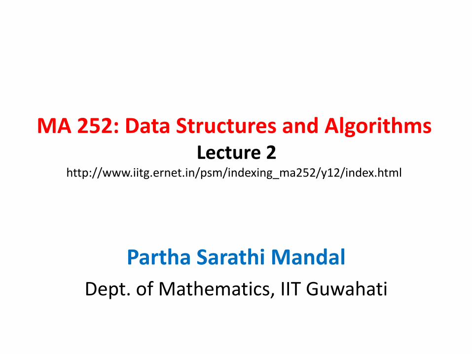
The problem of sorting
Input: sequence ⟨a1, a2, …, an⟩ of numbers.
Output: permutation ⟨a'1, a'2, …, a'n⟩ such that a'1≤a'2≤…≤a'n.
Example:
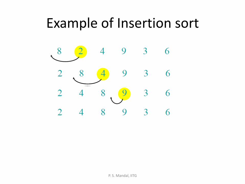
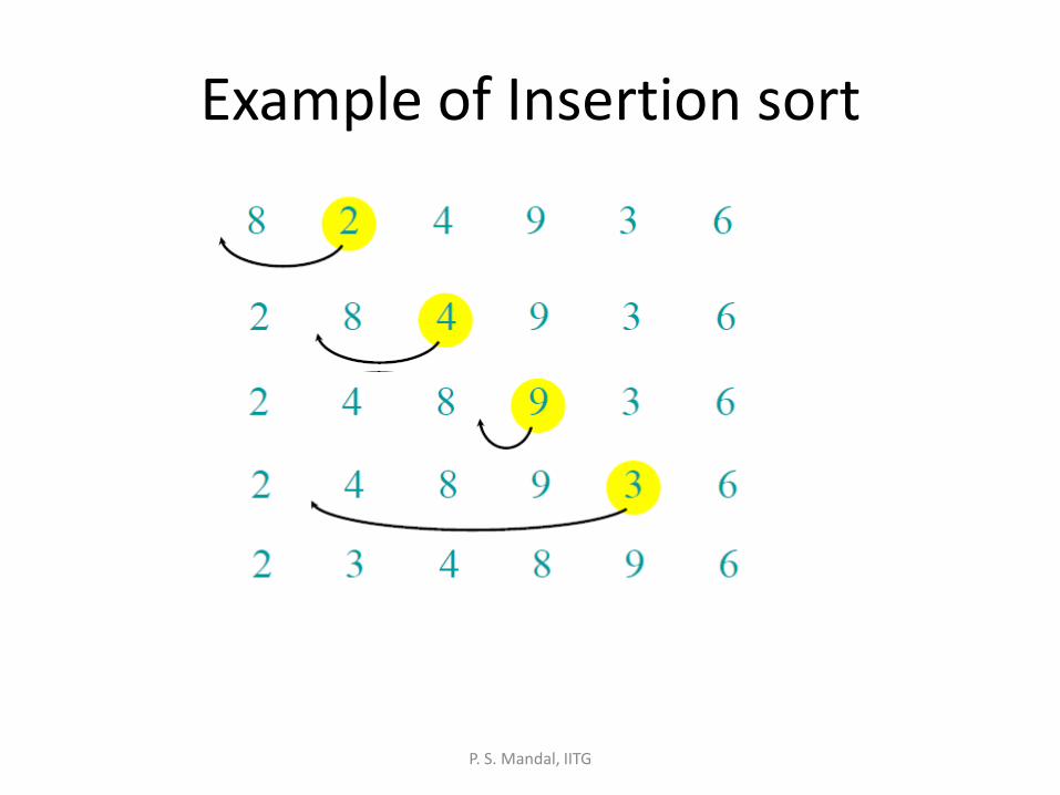
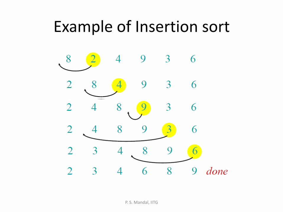
Input: 8 2 4 9 3 6
Output: 2 3 4 6 8 9
P. S. Mandal, IITG
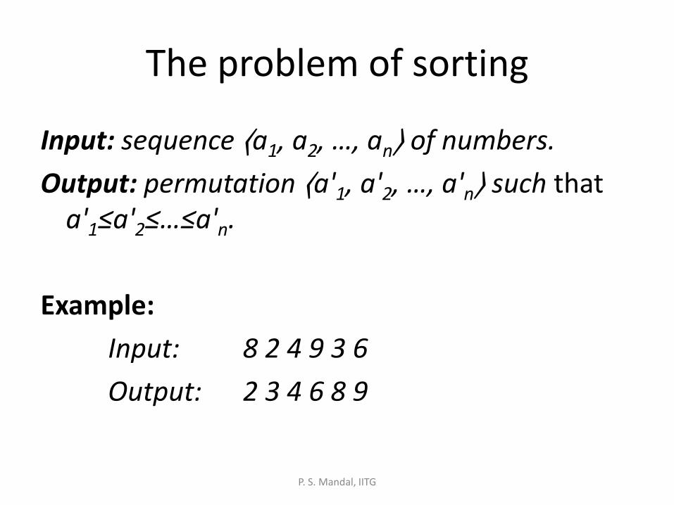
Sorting a hand of cards using insertion sort
P. S. Mandal, IITG
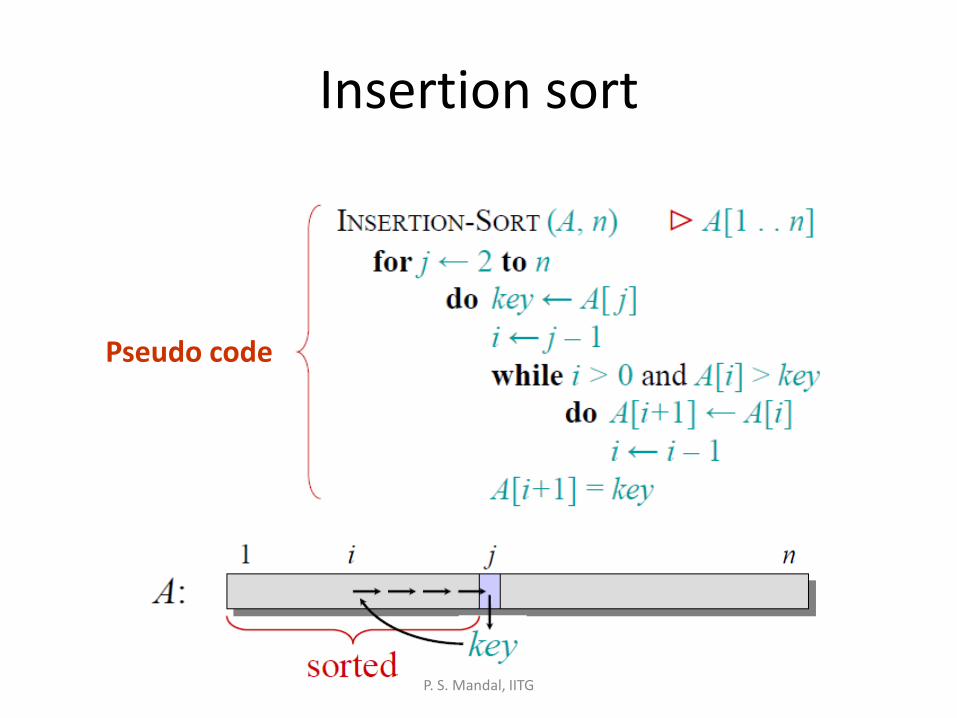
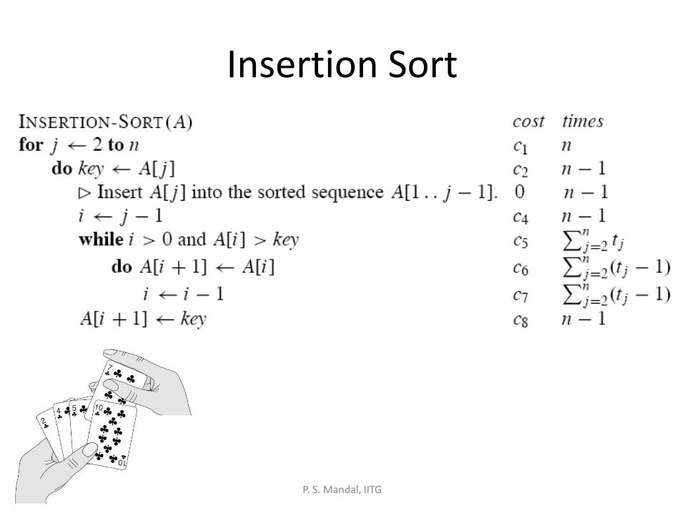
Insertion sort
Pseudo code
P. S. Mandal, IITG
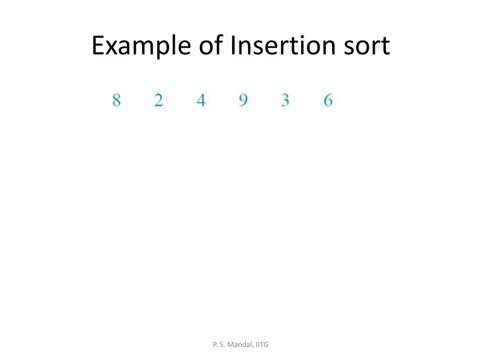
Example of Insertion sort
P. S. Mandal, IITG
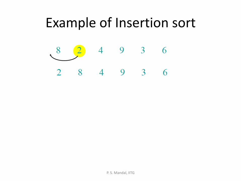
Example of Insertion sort
P. S. Mandal, IITG
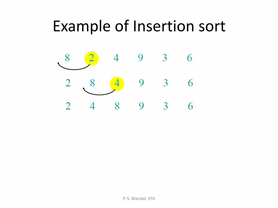
Example of Insertion sort
P. S. Mandal, IITG
Example of Insertion sort
P. S. Mandal, IITG
Example of Insertion sort
P. S. Mandal, IITG
Example of Insertion sort
P. S. Mandal, IITG

Running Time
• The running time depends on the input: an already sorted sequence is easier to sort.
• Parameterize the running time by the size of the input, since short sequences are easier to sort than long ones.
• Generally, we seek upper bounds on the running time, because everybody likes a guarantee.
P. S. Mandal, IITG
Insertion Sort
P. S. Mandal, IITG
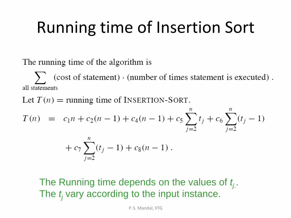
Running time of Insertion Sort
The Running time depends on the values of tj..
The tj vary according to the input instance.
P. S. Mandal, IITG

Best/Worst/Average Case
T(n) = (c1+c2+c4+c8)n + (c5+c6+c7) j=2j=n tj - (c2+c4+c6+c7+c8)
Best Case: when elements are already sorted then tj = 1, T(n) = f(n), linear time.
Worst Case: when elements are reversely sorted then tj = j, T(n) = f(n2), quadratic time
Average Case: when tj = j/2, T(n) = f(n2), quadratic time.
P. S. Mandal, IITG
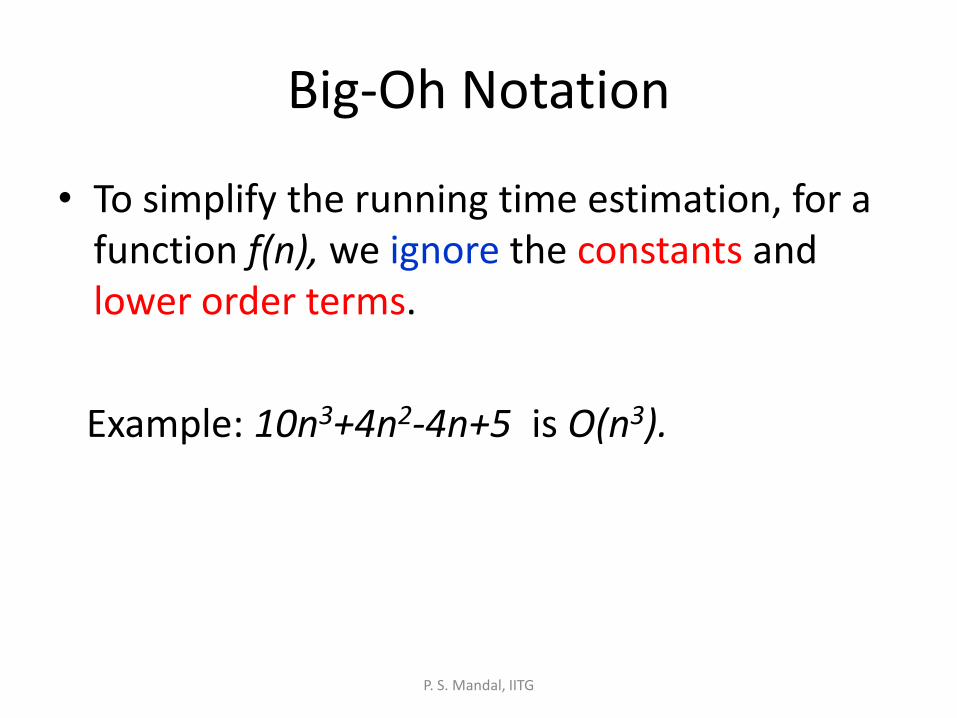
Big-Oh Notation
• To simplify the running time estimation, for a function f(n), we ignore the constants and lower order terms.
Example: 10n3+4n2-4n+5 is O(n3).
P. S. Mandal, IITG
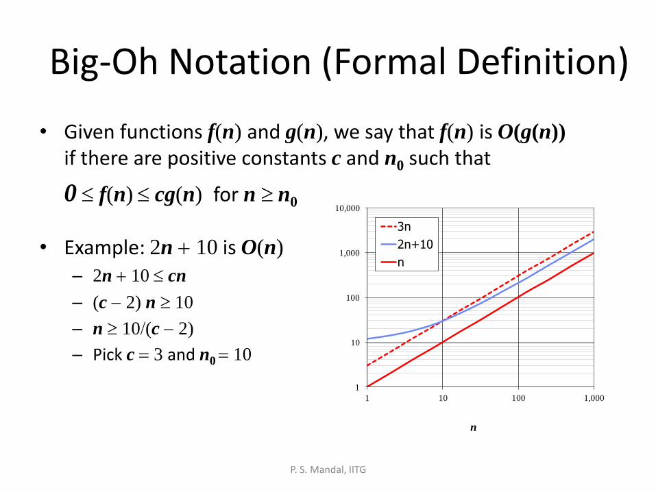
Big-Oh Notation (Formal Definition)
• Given functions f(n) and g(n), we say that f(n) is O(g(n)) if there are positive constants c and n0 such that
0 f(n) cg(n) for n n0
• Example: 2n + 10 is O(n)
– 2n + 10 cn
– (c 2) n 10
– n 10/(c 2)
– Pick c = 3 and n0 = 10
1
10
100
1,000
10,000
1 10 100 1,000
n
3n
2n+10
n
P. S. Mandal, IITG
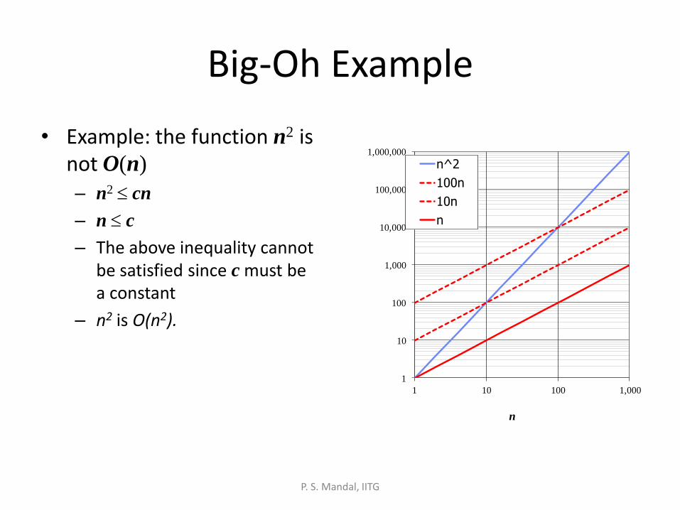
Big-Oh Example
• Example: the function n2 is not O(n)
– n2 cn
– n c
– The above inequality cannot be satisfied since c must be a constant
– n2 is O(n2).
1
10
100
1,000
10,000
100,000
1,000,000
1 10 100 1,000
n
n^2
100n
10n
n
P. S. Mandal, IITG
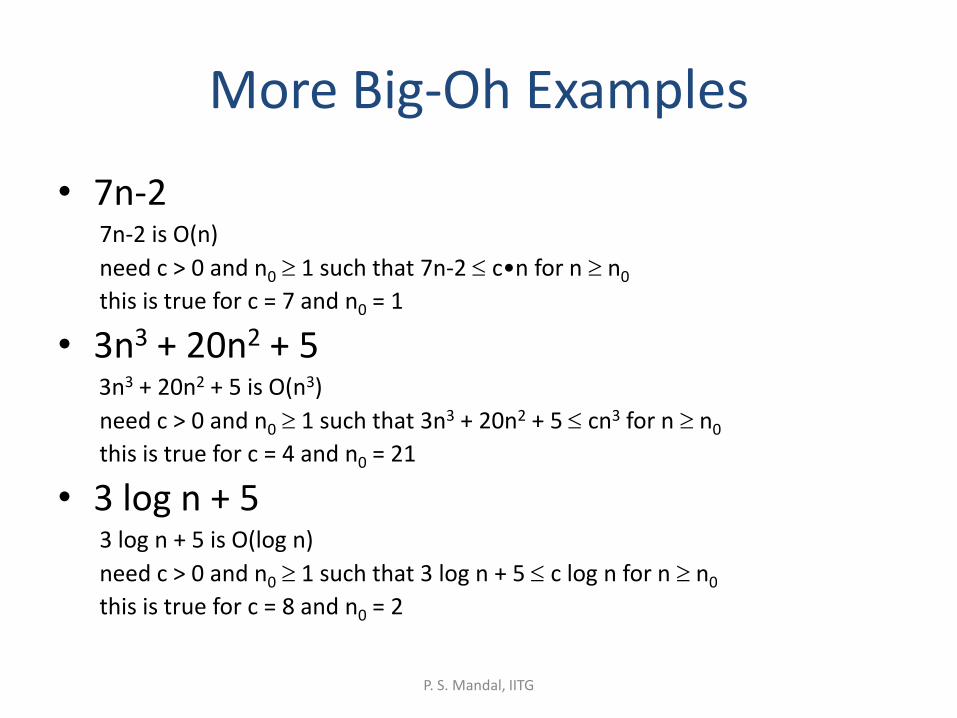
More Big-Oh Examples
• 7n-2 7n-2 is O(n)
need c > 0 and n0 1 such that 7n-2 c•n for n n0
this is true for c = 7 and n0 = 1
• 3n3 + 20n2 + 5 3n3 + 20n2 + 5 is O(n3)
need c > 0 and n0 1 such that 3n3 + 20n2 + 5 cn3 for n n0
this is true for c = 4 and n0 = 21
• 3 log n + 5 3 log n + 5 is O(log n)
need c > 0 and n0 1 such that 3 log n + 5 c log n for n n0
this is true for c = 8 and n0 = 2
P. S. Mandal, IITG
Big-Oh and Growth Rate
• The big-Oh notation gives an upper bound on the growth rate of a function
• The statement “f(n) is O(g(n))” means that the growth rate of f(n) is no more than the growth rate of g(n)
• We can use the big-Oh notation to rank functions according to their growth rate
P. S. Mandal, IITG
Big-Oh Rules
• If f(n) is a polynomial of degree d, then f(n) is O(nd), i.e., – Drop lower-order terms
– Drop constant factors
• Use the smallest possible class of functions
– Say “2n is O(n)” instead of “2n is O(n2)”
• Use the simplest expression of the class
– Say “3n + 5 is O(n)” instead of “3n + 5 is O(3n)”
P. S. Mandal, IITG
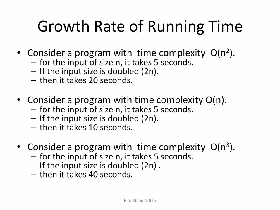
Growth Rate of Running Time
• Consider a program with time complexity O(n2). – for the input of size n, it takes 5 seconds. – If the input size is doubled (2n). – then it takes 20 seconds.
• Consider a program with time complexity O(n).
– for the input of size n, it takes 5 seconds. – If the input size is doubled (2n). – then it takes 10 seconds.
• Consider a program with time complexity O(n3).
– for the input of size n, it takes 5 seconds. – If the input size is doubled (2n) . – then it takes 40 seconds.
P. S. Mandal, IITG
Asymptotic Algorithm Analysis
• The asymptotic analysis of an algorithm determines the running time in big-Oh notation
• To perform the asymptotic analysis – We find the worst-case number of primitive operations executed as
a function of the input size
– We express this function with big-Oh notation
• Example: – We determine that algorithm arrayMax executes at most 6n 1
primitive operations
– We say that algorithm arrayMax “runs in O(n) time”
• Since constant factors and lower-order terms are eventually dropped anyhow, we can disregard them when counting primitive operations.
P. S. Mandal, IITG
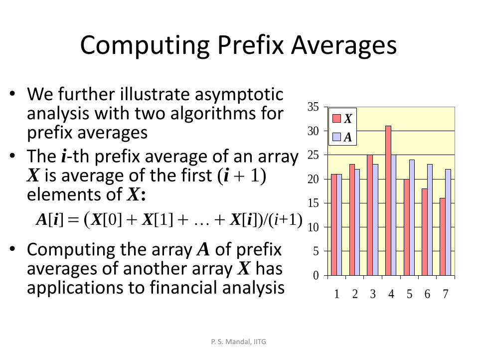
Computing Prefix Averages
• We further illustrate asymptotic analysis with two algorithms for prefix averages
• The i-th prefix average of an array X is average of the first (i + 1) elements of X:
A[i] = (X[0] + X[1] + … + X[i])/(i+1)
• Computing the array A of prefix averages of another array X has applications to financial analysis
0
5
10
15
20
25
30
35
1 2 3 4 5 6 7
X
A
P. S. Mandal, IITG
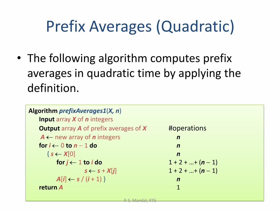
Prefix Averages (Quadratic)
• The following algorithm computes prefix averages in quadratic time by applying the definition.
Algorithm prefixAverages1(X, n) Input array X of n integers
Output array A of prefix averages of X #operations A new array of n integers n for i 0 to n 1 do n { s X[0] n for j 1 to i do 1 + 2 + …+ (n 1) s s + X[j] 1 + 2 + …+ (n 1) A[i] s / (i + 1) } n return A 1
P. S. Mandal, IITG
Arithmetic Progression
• The running time of prefixAverages1 is O(1 + 2 + …+ n)
• The sum of the first n integers is n(n + 1) / 2
– There is a simple visual proof of this fact
• Thus, algorithm prefixAverages1 runs in T(n)=O(n2) time
P. S. Mandal, IITG
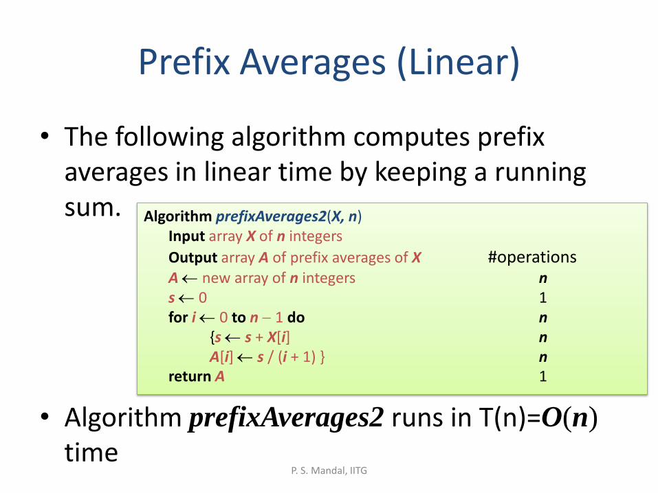
Prefix Averages (Linear)
• The following algorithm computes prefix averages in linear time by keeping a running sum.
• Algorithm prefixAverages2 runs in T(n)=O(n)
time
Algorithm prefixAverages2(X, n) Input array X of n integers
Output array A of prefix averages of X #operations A new array of n integers n s 0 1 for i 0 to n 1 do n {s s + X[i] n A[i] s / (i + 1) } n return A 1
P. S. Mandal, IITG


![[17] Mandal General Insurance_Batkhishig](https://img.pdfslide.us/doc/110x75/577cdfc81a28ab9e78b1f587/17-mandal-general-insurancebatkhishig.jpg)