MA-108 Ordinary Di erential Equations

MA-108 Ordinary Differential Equations

M.K. Keshari

Department of MathematicsIndian Institute of Technology Bombay

Powai, Mumbai - 76

19th March, 2015D3 - Lecture 6

M.K. Keshari D3 - Lecture 6

Recall: We saw some numerial methods to solve y′ = f(x, y)with y(x0) = y0.

Let h be the step size, i.e. xi = x0 + hi.

Euler’s method uses yi = yi−1 + hf(xi−1, yi−1).

Improved Euler Method uses

yi+1 = yi +h

2[f(xi, yi) + f(xi+1, yi + hf(xi, yi)) ].

Runge Kutta Method is the most widely used approximationmethod.For MA 108 exam purpose, we will only consider Euler andInproved Euler.

Now we will consider 2nd order linear ODE.


Solving IVP’s

The function L : C2(I)→ C(I) defined by

L(f) = f ′′ + p(x)f ′ + q(x)f

is a linear transformation. The null space of L,N(L) = {f ∈ C2(I) | L(f) = 0} consists of solutions of ODE

y′′ + p(x)y′ + q(x)y = 0.

Theorem (Uniqueness Theorem to homogeneous IVP)

Consider the homogeneous IVP

y′′ + p(x)y′ + q(x)y = 0, y(x0) = a, y′(x0) = b,

where p(x) and q(x) are continuous on an interval Icontaining x0. Then there is a unique solution to the IVP on I.


Ex. Find the largest interval where the ODE

x2y′′ + xy′ − 4y = 0

with initial condition y(x0) = y0 has a unique solution.

Write the ODE in standard form

y′′ + p(x)y′ + q(x)y = 0

where p(x) =1

xand q(x) =

−4x2

. Since p(x) and q(x) are

continuous on (−∞, 0) ∪ (0,∞), the IVP has has a uniquesolution on (−∞, 0) if x0 < 0 and on (0,∞) if x0 > 0.

• Verify that y1 = x2 is a solution of ODE on (−∞,∞) and

y2 =1

x2is a solution on (−∞, 0) ∪ (0,∞).


Ex. Solve IVP x2y′′ + xy′ − 4y = 0, y(1) = 2, y′(1) = 0.

Since y(x) = c1x2 + c2

1

x2is a solution of ODE. Find c1 and c2

using initial conditions.

We get c1 + c2 = 2, 2c1 − 2c2 = 0.

This gives c1 = 1 and c2 = 1.

Thus solution of IVP is

y(x) = x2 +1

x2

which is unique on the interval (0,∞). �

Ex. Solve x2y′′ + xy′ − 4y = 0, y(−1) = 2, y′(−1) = 0


Dimension Theorem

DIMENSION THEOREM:

If p(x), q(x) are continuous on an open interval I, then the setof solutions of the ODE

y′′ + p(x)y′ + q(x)y = 0 (1)

on I is a vector space of dimension 2. Any basis {y1, y2} ofsolutions of (1) is called a fundamental solutions of (1) �

• The theorem says that once you know that ex and e−x aresolutions of y′′ − y = 0 (1), any other solution will be of theform y(x) = c1e

x + c2e−x. Here {ex, e−x} is a fundamental

solutions of (1).

• Similarly, any solution of y′′ + y = 0 (1) are of the formy(x) = c1 sinx+ c2 cosx. Here {sinx, cosx} is fundamentalsolutions of (1).


Proof of Dimension Theorem

If y1 and y2 are solutions of (1), then c1y1 + c2y2 is also asolution of (1). To see this,

(c1y1 + c2y2)′′ + p(x)(c1y1 + c2y2)

′ + q(x)(c1y1 + c2y2) =

c1[y′′1 + p(x)y′1 + q(x)y1] + c2[y

′′2 + p(x)y′2 + q(x)y2] = 0

Thus the solution space is a vector space. Now

(i) we need to produce two linearly independent solutions, sayf and g, and

(ii) show that any other solution is a linear combination of fand g.


Proof of Dimension Theorem Continued ...

(i) Proof of existence of f and g

Fix x0 ∈ I. Let y1 = f(x) be the unique solution of the IVP

y′′ + p(x)y′ + q(x)y = 0, y(x0) = 1, y′(x0) = 0

y1 exists on I by uniqueness theorem. Similarly, let y2 = g(x)be the unique solution of the IVP

y′′ + p(x)y′ + q(x)y = 0, y(x0) = 0, y′(x0) = 1

We need to show that f, g are linearly independent. Assume

af(x) + bg(x) ≡ 0 =⇒ af ′(x) + bg′(x) ≡ 0

for some scalars a and b. Evaluate at x = x0, we get

a = 0, b = 0

This proves f and g are linearly independent. Now we show(ii) that any solution is a linear combination of f and g.


Proof of Dimension Theorem Continued ...

Let h(x) be an arbitrary solution of the given ODE. We wantto find c and d in R such that

h(x) = cf(x) + dg(x) =⇒ h′(x) = cf ′(x) + dg′(x) on I

Therefore, evaluating at x = x0 gives

h(x0) = cf(x0)+dg(x0) = c and h′(x0) = cf ′(x0)+dg′(x0) = d

Let h̃(x) = h(x0)f(x)+h′(x0)g(x). Then h̃(x) is a solution of

y′′+p(x)y′+q(x)y = 0, h̃(x0) = h(x0), h̃′(x0) = h′(x0) (2)

Since h(x) is also a solution of IVP (2), by uniqueness

theorem, h̃ = h. Thus any solution is a linear combination off and g. Therefore the solution space is 2-dimensional. �


Nonhomogeneous 2nd order linear ODE

Consider 2nd order linear ODE y′′ + p(x)y′ + q(x)y = r(x)(1)with p(x), q(x), r(x) continuous on open interval I.

The homogeneous part is y′′ + p(x)y′ + q(x)y = 0 (2)

We have seen that solution space of (2) is a 2-dimensionalvector space.(i) Suppose y1 is a solution of (1) and y2 is a solution of (2).Then y1 + y2 is a solution of (2). To see this

(y1 + y2)′′ + p(x)(y1 + y2)

′ + q(x)(y1 + y2) =

(y′′1 + p(x)y′1 + q(x)y1) + (y′′2 + p(x)y′2 + q(x)y2)

= r(x) + 0 = r(x).

(ii) Fix a solution y1 of (1). If y is a solution of (1), theny = y1 + y2, for some solution y2 of (2).

To see this, note that y − y1 is a solution of (2). Cally − y1 = y2. Then y = y1 + y2.


1 140260012 KALANTRE SANDESH SACHIN2 140260025 STHITAPRAGYAN MOHANTY3 14B030016 ABHISHEK JORWAL4 14D100002 VAIBHAV UMAKANT NEHETE5 14D100014 ADITYA KALRA6 14D260007 SHIVAM GARG7 140100042 SHIKHAR BUDHIRAJA8 140100007 UTKARSH GUPTA9 140100012 PRASADE RISHIKESH VINAY10 140100038 ASHMAK MOON11 140100050 MITALI ANIL MEDHE12 140100060 YASH DHOBLE13 140100074 PRASHANT KUMAR VARUN14 140100097 PATURU VENKATA SAI15 140100110 RAUNAQ BHIRANGI16 140260006 SHEETAL JAIN17 140260017 ZULFIQAR ALI18 140260029 VISHNU SAJ19 14B030017 SHIVANI CHOUDHARY


Wronskian and Linear Independence

Given two solutions f and g of y′′ + p(x)y′ + q(x)y = 0. Howto check whether f and g are linearly independent?We have seen in numerical method that evaluating a solutionat some point may not be possible. We start with a definitionfor this purpose.

Definition

Let f and g be two differentiable functions on I. TheWronskian of f(x) and g(x) is a function defined by

W (f, g;x) :=

∣∣∣∣ f(x) g(x)f ′(x) g′(x)

∣∣∣∣ = f(x)g′(x)− g(x)f ′(x).

Ex 1. Find Wronskian of ex and e−x at x = 0.W (ex, e−x, 0) = ex(−e−x)− e−xex|x=0 = −2.

2.W (sinx, cosx, 0) = sinx(− sinx)− cosx(cosx)|x=0 = −1.



Theorem (Abel’s Formula)

Assume p(x) and q(x) are continuous on I = (a, b). Let f(x)and g(x) be solutions of y′′ + p(x)y′ + q(x)y = 0.Then Wronskian of f(x) and g(x) is given by

W (f, g;x) = W (f, g; a) e−∫ xa p(t)dt,

for any a ∈ I.

Proof. Set W (f, g;x) = W (x). Then

W (x) = (fg′ − f ′g)(x).

Hence

W ′(x) = (fg′′ + f ′g′)− (f ′g′ + f ′′g)(x) = (fg′′ − f ′′g)(x)



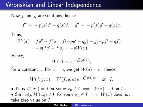
Now f and g are solutions, hence

f ′′ = − p(x)f ′ − q(x)f, g′′ = − p(x)g′ − q(x)g.

Thus,

W ′(x) = fg′′ − f ′′g = f(−pg′ − qg)− g(−pf ′ − qf)

= −p(fg′ − f ′g) = −pW (x).

Hence,W (x) = ce−

∫ xa p(t)dt,

for a constant c. For x = a, we get W (a) = c. Hence,

W (f, g;x) = W (f, g; a) e−∫ xa p(t)dt on I.

• Thus W (x0) = 0 for some x0 ∈ I =⇒ W (x) ≡ 0 on I.• Similarly, W (x0) 6= 0 for some x0 ∈ I =⇒ W (x) does nottake zero value on I.


Ex. Consider ODE x2y′′ + xy′ − 4y = 0.

Here y1 = x2 and y2 =1

x2are solutions. Compute the

Wronskian W (y1, y2;x).

Direct method: W = y1y′2− y′1y2 = x2(

−2x3

)− (2x)1

x2=−4x

.

Let’s verify Abel’s Formula: If x0 and x both are in (−∞, 0)or in (0,∞), then

W (x) = W (x0) exp

[−∫ x

x0

p(t) dt

]= W (x0) exp

[∫ x

x0

−1t

dt

]

= W (x0) exp [−(ln |x| − ln |x0|)] = W (x0) exp(lnx0

x)

=−4x0

x0

x= −4/x



Proposition

Suppose f(x) and g(x) are linearly dependent anddifferentiable on I = (a, b). Then, W (f, g;x) = 0 for allx ∈ I.

Proof. As f(x) and g(x) are linearly dependent, there existc, d ∈ R, not both 0, such that

cf(x) + dg(x) = 0 =⇒ cf ′(x) + dg′(x) = 0.

Hence, (f(x) g(x)f ′(x) g′(x)

) (cd

)=

(00

).

Since

(cd

)6=(00

), W (f, g;x0) = 0 for all x0 ∈ I. �



Note: The converse is not true, i.e. it may happen thatW (f, g, x) ≡ 0 on I, but f and g are linearly independent.

Ex. f(x) = x2 and

g(x) =

{x2 if x ≥ 0

−x2 if x < 0,

then, check that W (f, g;x) = 0 for all x ∈ R.But f and g are linearly independent.

Show that af + bg ≡ 0 =⇒ a = 0 = b. �

• In the next slide, we’ll see a correct formulation of theconverse.


Theorem

Considery′′ + p(x)y′ + q(x)y = 0,

where p(x) and q(x) are continuous on I = (a, b). Suppose fand g are solutions on I. Then f and g are linearlyindependent on I if and only if W (f, g;x) has no zeros in I.

Proof. (i) (⇒). It is enough to show that if W (x0) = 0 forsome x0 ∈ I, then f and g are linearly dependent.

Since f, g are linearly independent, f(x0) 6= 0 for some x0 ∈ I.

Choose an open interval J containing x0 such that f does nottake zero value on J . On J , we have:(

g

f

)′(x) =

(fg′ − f ′g

f 2

)(x) =

W (f, g;x)

f 2(x)= 0

since W (x0) = 0 =⇒ W (x) = W (x0)e∫ xx0−p(t)dt ≡ 0.


Proof continued ...

(g

f

)′≡ 0 on J =⇒ g

f= k

a constant on J . Hence g(x) = kf(x) on J .

But we want g(x) = kf(x) on I. For this, consider the IVP

y′′ + p(x)y′ + q(x)y = 0, y(x0) = 0, y′(x0) = 0 (∗)

y1 ≡ 0 and y2 = g − kf both are solutions of (*). Byuniqueness theorem, y1 = y2 on I. Hence g(x) = kf(x) on I.

Now we have to prove (⇐). It is enough to show that if f andg are linearly dependent, then W (f, g, ;x) ≡ 0. This is provedearlier. �



Remarks:

1 The continuity of p(x) and q(x) is required in the abovetheorem. Consider the DE

x2y′′ − 4xy′ + 6y = 0.

Then, x2 and x3 are linearly independent solutions, butW (x2, x3; 0) = 0.

2 W (f, g; a) = 0 for some a with {f, g} linearlyindependent implies that f and g together are notsolutions of an ODE on any interval containing a.

3 Similar is the case if Wronskian is zero at a point and notidentically zero.


Second Order Linear ODE’s

Consider second order linear homogeneous ODE

y′′ + p(x)y′ + q(x)y = 0.

As we remarked earlier, there is no general method to find abasis of solutions. However, if we know one non-zero solutionf(x), then we have a method to find another solution g(x)such that f(x) and g(x) are linearly independent.To find such a g(x), set

g(x) = v(x)f(x).

We’ll choose v such that f and g will be linearly independent.Can v be a constant? No. Now for g to be a solution of thegiven ODE, we need g′′ + p(x)g′ + q(x)g = 0.

=⇒ (vf)′′ + p(x)(vf)′ + q(x)(vf) = 0.M.K. Keshari D3 - Lecture 6


=⇒ (v′f + vf ′)′ + p(v′f + vf ′) + qvf = 0

=⇒ (v′′f + 2v′f ′ + vf ′′) + p(v′f + vf ′) + qvf = 0

=⇒ v(f ′′ + pf ′ + qf) + v′(2f ′ + pf) + v′′f = 0

=⇒ v′(2f ′ + pf) + v′′f = 0

Thus,v′′

v′= − 2f ′ + pf

f= −2f ′

f− p.

Therefore,

ln |v′| = ln

(1

f 2

)−∫

pdx;

=⇒ v =

∫e−

∫pdx

f 2dx.



Claim: f and vf are linearly independent.

Enough to check Wronskian!

W (f, vf) = f(v′f + f ′v)− f ′vf

= f 2v′ = f 2 e−

∫pdx

f 2= e−

∫pdx 6= 0

Theorem

If y1 is one solution of y′′ + p(x)y′ + q(x)y = 0, then anothersolution is given by

y2(x) = vy1(x) = (

∫e−

∫pdx

y21dx)y1(x)



Example: Find all solutions of

x2y′′ + xy′ − y = 0.

Given that f(x) = x is one solution.

Write this in standard form:

y′′ +y′

x− y

x2= 0.

Let g = vf = vx be another solution. Then,

v(x) =

∫e−

∫pdx

f 2dx =

∫e−

∫dxx

x2dx =

∫dx

x3= − 1

2x2.

Hence, any solution is of the form cx+d

xfor c, d ∈ R.


Documents

MA-108 Ordinary Di erential Equations