M3D-RPN: Monocular 3D Region Proposal Network for Object Detection

Garrick Brazil, Xiaoming Liu

Michigan State University, East Lansing MI

{brazilga, liuxm}@msu.edu

Abstract

Understanding the world in 3D is a critical component

of urban autonomous driving. Generally, the combination

of expensive LiDAR sensors and stereo RGB imaging has

been paramount for successful 3D object detection algo-

rithms, whereas monocular image-only methods experience

drastically reduced performance. We propose to reduce the

gap by reformulating the monocular 3D detection problem

as a standalone 3D region proposal network. We leverage

the geometric relationship of 2D and 3D perspectives, al-

lowing 3D boxes to utilize well-known and powerful con-

volutional features generated in the image-space. To help

address the strenuous 3D parameter estimations, we fur-

ther design depth-aware convolutional layers which enable

location specific feature development and in consequence

improved 3D scene understanding. Compared to prior work

in monocular 3D detection, our method consists of only the

proposed 3D region proposal network rather than relying

on external networks, data, or multiple stages. M3D-RPN

is able to significantly improve the performance of both

monocular 3D Object Detection and Bird’s Eye View tasks

within the KITTI urban autonomous driving dataset, while

efficiently using a shared multi-class model.

1. Introduction

Scene understanding in 3D plays a principal role in de-

signing effective real-world systems such as in urban au-

tonomous driving [2, 10, 15] and robotics [17, 36]. Cur-

rently, the foremost methods [12, 24, 31, 35, 41] on 3D de-

tection rely extensively on expensive LiDAR sensors to pro-

vide sparse depth data as input. In comparison, monocular

image-only 3D detection [7, 8, 28, 40] is considerably more

difficult due to an inherent lack of depth cues. As a conse-

quence, the performance gap between LiDAR-based meth-

ods and monocular approaches remains substantial.

Prior work on monocular 3D detection have each relied

heavily on external state-of-the-art (SOTA) sub-networks,

which are individually responsible for performing point

cloud generation [8], semantic segmentation [7], 2D detec-

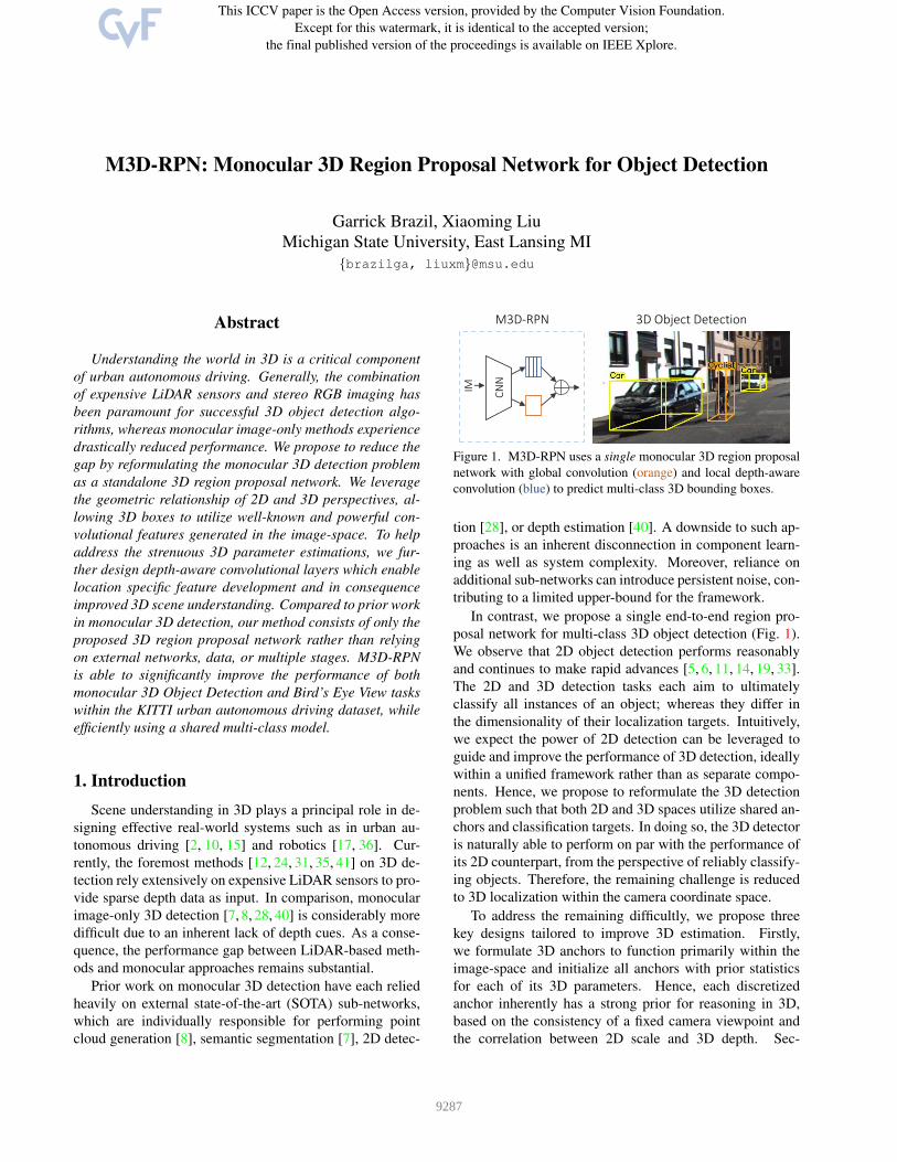
CN

N

IM

M3D-RPN 3D Object Detection

Figure 1. M3D-RPN uses a single monocular 3D region proposal

network with global convolution (orange) and local depth-aware

convolution (blue) to predict multi-class 3D bounding boxes.

tion [28], or depth estimation [40]. A downside to such ap-

proaches is an inherent disconnection in component learn-

ing as well as system complexity. Moreover, reliance on

additional sub-networks can introduce persistent noise, con-

tributing to a limited upper-bound for the framework.

In contrast, we propose a single end-to-end region pro-

posal network for multi-class 3D object detection (Fig. 1).

We observe that 2D object detection performs reasonably

and continues to make rapid advances [5, 6, 11, 14, 19, 33].

The 2D and 3D detection tasks each aim to ultimately

classify all instances of an object; whereas they differ in

the dimensionality of their localization targets. Intuitively,

we expect the power of 2D detection can be leveraged to

guide and improve the performance of 3D detection, ideally

within a unified framework rather than as separate compo-

nents. Hence, we propose to reformulate the 3D detection

problem such that both 2D and 3D spaces utilize shared an-

chors and classification targets. In doing so, the 3D detector

is naturally able to perform on par with the performance of

its 2D counterpart, from the perspective of reliably classify-

ing objects. Therefore, the remaining challenge is reduced

to 3D localization within the camera coordinate space.

To address the remaining difficultly, we propose three

key designs tailored to improve 3D estimation. Firstly,

we formulate 3D anchors to function primarily within the

image-space and initialize all anchors with prior statistics

for each of its 3D parameters. Hence, each discretized

anchor inherently has a strong prior for reasoning in 3D,

based on the consistency of a fixed camera viewpoint and

the correlation between 2D scale and 3D depth. Sec-

9287

ondly, we design a novel depth-aware convolutional layer

which is able to learn spatially-aware features. Tradition-

ally, convolutional operations are preferred to be spatially-

invariant [21, 22] in order to detect objects at arbitrary im-

age locations. However, while it is likely beneficial for

low-level features, we show that high-level features improve

when given increased awareness of their depth and while as-

suming a consistent camera scene geometry. Lastly, we op-

timize the orientation estimation θ using 3D→ 2D projec-

tion consistency loss within a post-optimization algorithm.

Hence, helping correct anomalies within θ estimation while

assuming a reliable 2D bounding box.

To summarize, our contributions are the following:

• We formulate a standalone monocular 3D region pro-

posal network (M3D-RPN) with a shared 2D and 3D

detection space, while using prior statistics to serve as

strong initialization for each 3D parameter.

• We propose depth-aware convolution to improve the

3D parameter estimation, thereby enabling the net-

work to learn more spatially-aware high-level features.

• We propose a simple orientation estimation post-

optimization algorithm which uses 3D projections and

2D detections to improve the θ estimation.

• We achieve state-of-the-art performance on the urban

KITTI [15] benchmark for monocular Bird’s Eye View

and 3D Detection using a single multi-class network.

2. Related Work

2D Detection: Many works have addressed 2D detection

in both generic [20, 23, 25, 29, 32] and urban scenes [3–6,

26, 27, 33, 42, 45]. Most recent frameworks are based on

seminal work of Faster R-CNN [34] due to the introduction

of the region proposal network (RPN) as a highly effective

method to efficiently generate object proposals. The RPN

functions as a sliding window detector to check for the exis-

tence of objects at every spatial location of an image which

match with a set of predefined template shapes, referred to

as anchors. Despite that the RPN was conceived to be a

preliminary stage within Faster R-CNN, it is often demon-

strated to have promising effectiveness being extended to a

single-shot standalone detector [25, 32, 38, 44]. Our frame-

work builds upon the anchors of a RPN, specially designed

to function in both the 2D and 3D spaces, and acting as a

single-shot multi-class 3D detector.

LiDAR 3D Detection: The use of LiDAR data has proven

to be essential input for SOTA frameworks [9, 12, 13, 24,

31, 35, 41] for 3D object detection applied to urban scenes.

Leading methods tend to process sparse point clouds from

LiDAR points [31, 35, 41] or project the point clouds into

sets of 2D planes [9, 12]. While the LiDAR-based meth-

ods are generally high performing for a variety of 3D tasks,

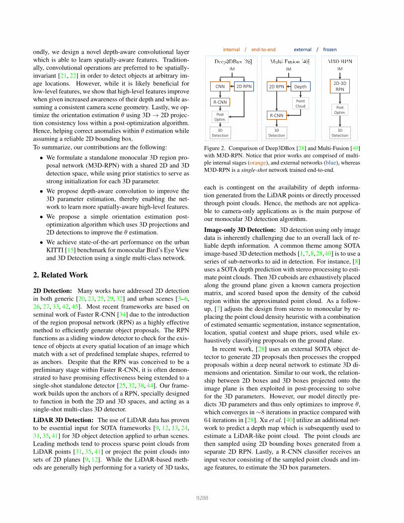
2D RPN

R-CNN

Post

Optim.

CNN

3D

Detection

IM

external / frozeninternal / end-to-end

R-CNN

2D RPN

3D

Detection

IM

Point

Cloud

3D

Detection

IM

Post

Optim.

Depth2D-3D

RPN

Figure 2. Comparison of Deep3DBox [28] and Multi-Fusion [40]

with M3D-RPN. Notice that prior works are comprised of multi-

ple internal stages (orange), and external networks (blue), whereas

M3D-RPN is a single-shot network trained end-to-end.

each is contingent on the availability of depth informa-

tion generated from the LiDAR points or directly processed

through point clouds. Hence, the methods are not applica-

ble to camera-only applications as is the main purpose of

our monocular 3D detection algorithm.

Image-only 3D Detection: 3D detection using only image

data is inherently challenging due to an overall lack of re-

liable depth information. A common theme among SOTA

image-based 3D detection methods [1,7,8,28,40] is to use a

series of sub-networks to aid in detection. For instance, [8]

uses a SOTA depth prediction with stereo processing to esti-

mate point clouds. Then 3D cuboids are exhaustively placed

along the ground plane given a known camera projection

matrix, and scored based upon the density of the cuboid

region within the approximated point cloud. As a follow-

up, [7] adjusts the design from stereo to monocular by re-

placing the point cloud density heuristic with a combination

of estimated semantic segmentation, instance segmentation,

location, spatial context and shape priors, used while ex-

haustively classifying proposals on the ground plane.

In recent work, [28] uses an external SOTA object de-

tector to generate 2D proposals then processes the cropped

proposals within a deep neural network to estimate 3D di-

mensions and orientation. Similar to our work, the relation-

ship between 2D boxes and 3D boxes projected onto the

image plane is then exploited in post-processing to solve

for the 3D parameters. However, our model directly pre-

dicts 3D parameters and thus only optimizes to improve θ,

which converges in∼8 iterations in practice compared with

64 iterations in [28]. Xu et al. [40] utilize an additional net-

work to predict a depth map which is subsequently used to

estimate a LiDAR-like point cloud. The point clouds are

then sampled using 2D bounding boxes generated from a

separate 2D RPN. Lastly, a R-CNN classifier receives an

input vector consisting of the sampled point clouds and im-

age features, to estimate the 3D box parameters.

9288

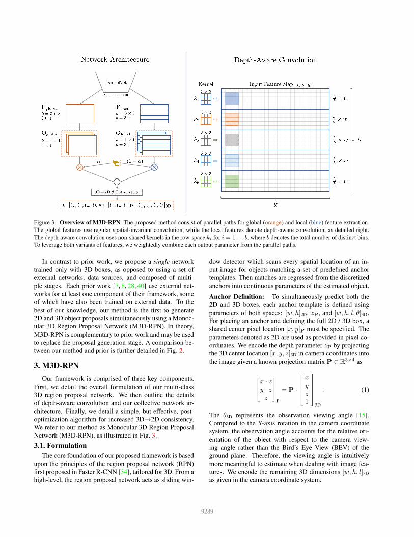
Figure 3. Overview of M3D-RPN. The proposed method consist of parallel paths for global (orange) and local (blue) feature extraction.

The global features use regular spatial-invariant convolution, while the local features denote depth-aware convolution, as detailed right.

The depth-aware convolution uses non-shared kernels in the row-space ki for i = 1 . . . b, where b denotes the total number of distinct bins.

To leverage both variants of features, we weightedly combine each output parameter from the parallel paths.

In contrast to prior work, we propose a single network

trained only with 3D boxes, as opposed to using a set of

external networks, data sources, and composed of multi-

ple stages. Each prior work [7, 8, 28, 40] use external net-

works for at least one component of their framework, some

of which have also been trained on external data. To the

best of our knowledge, our method is the first to generate

2D and 3D object proposals simultaneously using a Monoc-

ular 3D Region Proposal Network (M3D-RPN). In theory,

M3D-RPN is complementary to prior work and may be used

to replace the proposal generation stage. A comparison be-

tween our method and prior is further detailed in Fig. 2.

3. M3D-RPN

Our framework is comprised of three key components.

First, we detail the overall formulation of our multi-class

3D region proposal network. We then outline the details

of depth-aware convolution and our collective network ar-

chitecture. Finally, we detail a simple, but effective, post-

optimization algorithm for increased 3D→2D consistency.

We refer to our method as Monocular 3D Region Proposal

Network (M3D-RPN), as illustrated in Fig. 3.

3.1. Formulation

The core foundation of our proposed framework is based

upon the principles of the region proposal network (RPN)

first proposed in Faster R-CNN [34], tailored for 3D. From a

high-level, the region proposal network acts as sliding win-

dow detector which scans every spatial location of an in-

put image for objects matching a set of predefined anchor

templates. Then matches are regressed from the discretized

anchors into continuous parameters of the estimated object.

Anchor Definition: To simultaneously predict both the

2D and 3D boxes, each anchor template is defined using

parameters of both spaces: [w, h]2D, zP, and [w, h, l, θ]3D.

For placing an anchor and defining the full 2D / 3D box, a

shared center pixel location [x, y]P must be specified. The

parameters denoted as 2D are used as provided in pixel co-

ordinates. We encode the depth parameter zP by projecting

the 3D center location [x, y, z]3D in camera coordinates into

the image given a known projection matrix P ∈ R3×4 as

x · zy · zz

P

= P ·

xyz1

3D

. (1)

The θ3D represents the observation viewing angle [15].

Compared to the Y-axis rotation in the camera coordinate

system, the observation angle accounts for the relative ori-

entation of the object with respect to the camera view-

ing angle rather than the Bird’s Eye View (BEV) of the

ground plane. Therefore, the viewing angle is intuitively

more meaningful to estimate when dealing with image fea-

tures. We encode the remaining 3D dimensions [w, h, l]3D

as given in the camera coordinate system.

9289

Figure 4. Anchor Formulation and Visualized 3D Anchors. We depict each parameter of within the 2D / 3D anchor formulation (left).

We visualize the precomputed 3D priors when 12 anchors are used after projection in the image view (middle) and Bird’s Eye View (right).

For visualization purposes only, we span anchors in specific x3D locations which best minimize overlap when viewed.

The mean statistic for each zP and [w, h, l, θ]3D is pre-

computed for each anchor individually, which acts as strong

prior to ease the difficultly in estimating 3D parameters.

Specifically, for each anchor we use the statistics across

all matching ground truths which have ≥ 0.5 intersection

over union (IoU) with the bounding box of the correspond-

ing [w, h]2D anchor. As a result, the anchors represent dis-

cretized templates where the 3D priors can be leveraged as a

strong initial guess, thereby assuming a reasonably consis-

tent scene geometry. We visualize the anchor formulation

as well as precomputed 3D priors in Fig. 4.

3D Detection: Our model predicts output feature maps per

anchor for c, [tx, ty, tw, th]2D, [tx, ty, tz]P, [tw, th, tl, tθ]3D.

Let us denote na the number of anchors, nc the number of

classes, and h× w the feature map resolution. As such, the

total number of box outputs is denoted nb = w × h × na,

spanned at each pixel location [x, y]P ∈ Rw×h per anchor.

The first output c represents the shared classification predic-

tion of size na×nc×h×w, whereas each other output has

size na × h× w. The outputs of [tx, ty, tw, th]2D represent

the 2D bounding box transformation, which we collectively

refer to as b2D. Following [34], the bounding box transfor-

mation is applied to an anchor with [w, h]2D as:

x′

2D = xP + tx2D· w2D, w′

2D = exp(tw2D) · w2D,

y′2D = yP + ty2D· h2D, h′

2D = exp(th2D) · h2D,

(2)

where xP and yP denote spatial center location of each box.

The transformed box b′2D is thus defined as [x, y, w, h]′2D.

The following 7 outputs represent transformations denoting

the projected center [tx, ty, tz]P, dimensions [tw, th, tl]3D

and orientation tθ3D, which we collectively refer to as b3D.

Similar to 2D, the transformation is applied to an anchor

with parameters [w, h]2D, zP, and [w, h, l, θ]3D as follows:

x′

P= xP + txP

· w2D, w′

3D = exp(tw3D) · w3D,

y′P= yP + tyP

· h2D, h′

3D = exp(th3D) · h3D,

z′P= tzP + zP, l′3D = exp(tl3D

) · l3D,

θ′3D = tθ3D+ θ3D.

(3)

Hence, b′3D is then denoted as [x, y, z]′P

and [w, h, l, θ]′3D.

As described, we estimate the projected 3D center rather

than camera coordinates to better cope with the convolu-

tional features based exclusively in the image space. There-

fore, during inference we back-project the projected 3D

center location from the image space [x, y, z]′P

to camera

coordinates [x, y, z]′3D by using the inverse of Eqn. 1.

Loss Definition: The network loss of our framework is

formed as a multi-task learning problem composed of clas-

sification Lc and a box regression loss for 2D and 3D, re-

spectfully denoted as Lb2Dand Lb3D

. For each generated

box, we check if there exists a ground truth with at least

≥ 0.5 IoU, as in [34]. If yes then we use the best matched

ground truth for each generated box to define a target with

τ class index, 2D box b2D, and 3D box b3D. Otherwise, τis assigned to the catch-all background class and bounding

box regression is ignored. A softmax-based multinomial lo-

gistic loss is used to supervise for Lc defined as:

Lc = − log

(

exp(cτ )

Σnc

i exp(ci)

)

. (4)

We use a negative logistic loss applied to the IoU between

the matched ground truth box b2D and the transformed b′2D

for Lb2D, similar to [37, 43], defined as:

Lb2D= − log

(

IoU(b′2D, b2D))

. (5)

The remaining 3D bounding box parameters are each opti-

mized using a Smooth L1 [16] regression loss applied to the

transformations b3D and the ground truth transformations

g3D (generated using b3D following the inverse of Eqn. 3):

Lb3D= SmoothL1(b3D, g3D). (6)

Hence, the overall multi-task network loss L, including reg-

ularization weights λ1 and λ2, is denoted as:

L = Lc + λ1Lb2D+ λ2Lb3D

. (7)

9290

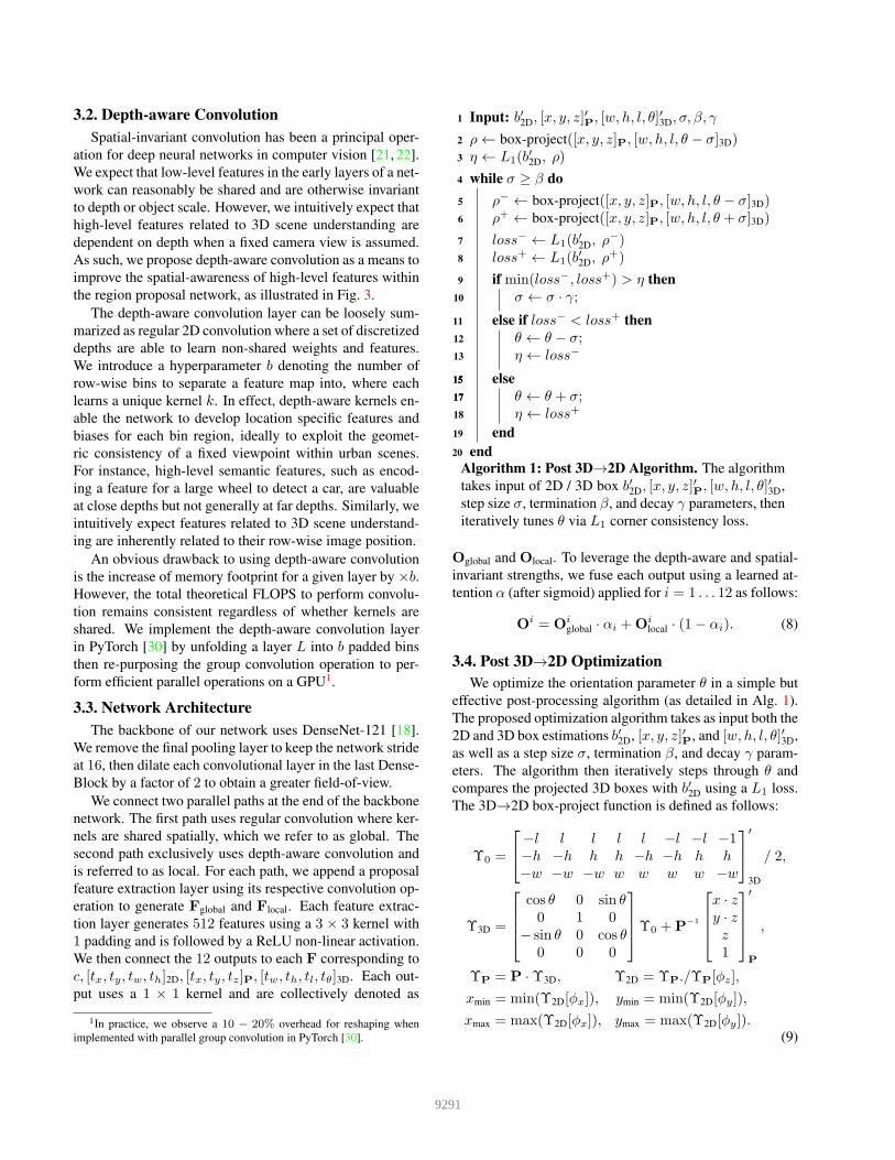
3.2. Depth­aware Convolution

Spatial-invariant convolution has been a principal oper-

ation for deep neural networks in computer vision [21, 22].

We expect that low-level features in the early layers of a net-

work can reasonably be shared and are otherwise invariant

to depth or object scale. However, we intuitively expect that

high-level features related to 3D scene understanding are

dependent on depth when a fixed camera view is assumed.

As such, we propose depth-aware convolution as a means to

improve the spatial-awareness of high-level features within

the region proposal network, as illustrated in Fig. 3.

The depth-aware convolution layer can be loosely sum-

marized as regular 2D convolution where a set of discretized

depths are able to learn non-shared weights and features.

We introduce a hyperparameter b denoting the number of

row-wise bins to separate a feature map into, where each

learns a unique kernel k. In effect, depth-aware kernels en-

able the network to develop location specific features and

biases for each bin region, ideally to exploit the geomet-

ric consistency of a fixed viewpoint within urban scenes.

For instance, high-level semantic features, such as encod-

ing a feature for a large wheel to detect a car, are valuable

at close depths but not generally at far depths. Similarly, we

intuitively expect features related to 3D scene understand-

ing are inherently related to their row-wise image position.

An obvious drawback to using depth-aware convolution

is the increase of memory footprint for a given layer by ×b.However, the total theoretical FLOPS to perform convolu-

tion remains consistent regardless of whether kernels are

shared. We implement the depth-aware convolution layer

in PyTorch [30] by unfolding a layer L into b padded bins

then re-purposing the group convolution operation to per-

form efficient parallel operations on a GPU1.

3.3. Network Architecture

The backbone of our network uses DenseNet-121 [18].

We remove the final pooling layer to keep the network stride

at 16, then dilate each convolutional layer in the last Dense-

Block by a factor of 2 to obtain a greater field-of-view.

We connect two parallel paths at the end of the backbone

network. The first path uses regular convolution where ker-

nels are shared spatially, which we refer to as global. The

second path exclusively uses depth-aware convolution and

is referred to as local. For each path, we append a proposal

feature extraction layer using its respective convolution op-

eration to generate Fglobal and Flocal. Each feature extrac-

tion layer generates 512 features using a 3 × 3 kernel with

1 padding and is followed by a ReLU non-linear activation.

We then connect the 12 outputs to each F corresponding to

c, [tx, ty, tw, th]2D, [tx, ty, tz]P, [tw, th, tl, tθ]3D. Each out-

put uses a 1 × 1 kernel and are collectively denoted as

1In practice, we observe a 10 − 20% overhead for reshaping when

implemented with parallel group convolution in PyTorch [30].

1 Input: b′2D, [x, y, z]′

P, [w, h, l, θ]′3D, σ, β, γ

2 ρ← box-project([x, y, z]P, [w, h, l, θ − σ]3D)3 η ← L1(b

′

2D, ρ)

4 while σ ≥ β do

5 ρ− ← box-project([x, y, z]P, [w, h, l, θ − σ]3D)6 ρ+ ← box-project([x, y, z]P, [w, h, l, θ + σ]3D)

7 loss− ← L1(b′

2D, ρ−)

8 loss+ ← L1(b′

2D, ρ+)

9 if min(loss−, loss+) > η then

10 σ ← σ · γ;

11 else if loss− < loss+ then

12 θ ← θ − σ;13 η ← loss−

1515 else

1717 θ ← θ + σ;18 η ← loss+

19 end

20 end

Algorithm 1: Post 3D→2D Algorithm. The algorithm

takes input of 2D / 3D box b′2D, [x, y, z]′

P, [w, h, l, θ]′3D,

step size σ, termination β, and decay γ parameters, then

iteratively tunes θ via L1 corner consistency loss.

Oglobal and Olocal. To leverage the depth-aware and spatial-

invariant strengths, we fuse each output using a learned at-

tention α (after sigmoid) applied for i = 1 . . . 12 as follows:

Oi = O

iglobal · αi +O

ilocal · (1− αi). (8)

3.4. Post 3D→2D Optimization

We optimize the orientation parameter θ in a simple but

effective post-processing algorithm (as detailed in Alg. 1).

The proposed optimization algorithm takes as input both the

2D and 3D box estimations b′2D, [x, y, z]′P

, and [w, h, l, θ]′3D,

as well as a step size σ, termination β, and decay γ param-

eters. The algorithm then iteratively steps through θ and

compares the projected 3D boxes with b′2D using a L1 loss.

The 3D→2D box-project function is defined as follows:

Υ0 =

−l l l l l −l −l −1−h −h h h −h −h h h−w −w −w w w w w −w

′

3D

/ 2,

Υ3D =

cos θ 0 sin θ0 1 0

− sin θ 0 cos θ0 0 0

Υ0 +P−1

x · zy · zz1

′

P

,

ΥP = P ·Υ3D, Υ2D = ΥP./ΥP[φz],

xmin = min(Υ2D[φx]), ymin = min(Υ2D[φy]),

xmax = max(Υ2D[φx]), ymax = max(Υ2D[φy]).(9)

9291

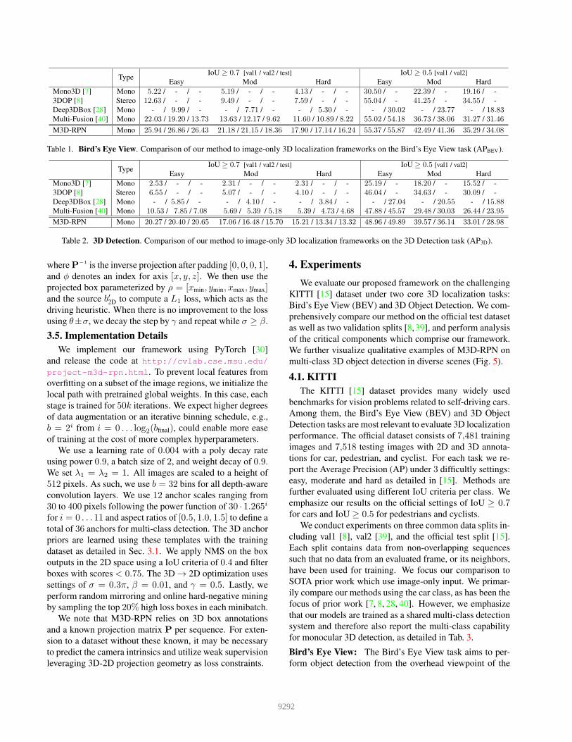
TypeIoU ≥ 0.7 [val1 / val2 / test] IoU ≥ 0.5 [val1 / val2]

Easy Mod Hard Easy Mod Hard

Mono3D [7] Mono 5.22 / - / - 5.19 / - / - 4.13 / - / - 30.50 / - 22.39 / - 19.16 / -

3DOP [8] Stereo 12.63 / - / - 9.49 / - / - 7.59 / - / - 55.04 / - 41.25 / - 34.55 / -

Deep3DBox [28] Mono - / 9.99 / - - / 7.71 / - - / 5.30 / - - / 30.02 - / 23.77 - / 18.83Multi-Fusion [40] Mono 22.03 / 19.20 / 13.73 13.63 / 12.17 / 9.62 11.60 / 10.89 / 8.22 55.02 / 54.18 36.73 / 38.06 31.27 / 31.46

M3D-RPN Mono 25.94 / 26.86 / 26.43 21.18 / 21.15 / 18.36 17.90 / 17.14 / 16.24 55.37 / 55.87 42.49 / 41.36 35.29 / 34.08

Table 1. Bird’s Eye View. Comparison of our method to image-only 3D localization frameworks on the Bird’s Eye View task (APBEV).

TypeIoU ≥ 0.7 [val1 / val2 / test] IoU ≥ 0.5 [val1 / val2]

Easy Mod Hard Easy Mod Hard

Mono3D [7] Mono 2.53 / - / - 2.31 / - / - 2.31 / - / - 25.19 / - 18.20 / - 15.52 / -

3DOP [8] Stereo 6.55 / - / - 5.07 / - / - 4.10 / - / - 46.04 / - 34.63 / - 30.09 / -

Deep3DBox [28] Mono - / 5.85 / - - / 4.10 / - - / 3.84 / - - / 27.04 - / 20.55 - / 15.88Multi-Fusion [40] Mono 10.53 / 7.85 / 7.08 5.69 / 5.39 / 5.18 5.39 / 4.73 / 4.68 47.88 / 45.57 29.48 / 30.03 26.44 / 23.95

M3D-RPN Mono 20.27 / 20.40 / 20.65 17.06 / 16.48 / 15.70 15.21 / 13.34 / 13.32 48.96 / 49.89 39.57 / 36.14 33.01 / 28.98

Table 2. 3D Detection. Comparison of our method to image-only 3D localization frameworks on the 3D Detection task (AP3D).

where P−1 is the inverse projection after padding [0, 0, 0, 1],and φ denotes an index for axis [x, y, z]. We then use the

projected box parameterized by ρ = [xmin, ymin, xmax, ymax]and the source b′2D to compute a L1 loss, which acts as the

driving heuristic. When there is no improvement to the loss

using θ±σ, we decay the step by γ and repeat while σ ≥ β.

3.5. Implementation Details

We implement our framework using PyTorch [30]

and release the code at http://cvlab.cse.msu.edu/

project-m3d-rpn.html. To prevent local features from

overfitting on a subset of the image regions, we initialize the

local path with pretrained global weights. In this case, each

stage is trained for 50k iterations. We expect higher degrees

of data augmentation or an iterative binning schedule, e.g.,

b = 2i from i = 0 . . . log2(bfinal), could enable more ease

of training at the cost of more complex hyperparameters.

We use a learning rate of 0.004 with a poly decay rate

using power 0.9, a batch size of 2, and weight decay of 0.9.

We set λ1 = λ2 = 1. All images are scaled to a height of

512 pixels. As such, we use b = 32 bins for all depth-aware

convolution layers. We use 12 anchor scales ranging from

30 to 400 pixels following the power function of 30 · 1.265i

for i = 0 . . . 11 and aspect ratios of [0.5, 1.0, 1.5] to define a

total of 36 anchors for multi-class detection. The 3D anchor

priors are learned using these templates with the training

dataset as detailed in Sec. 3.1. We apply NMS on the box

outputs in the 2D space using a IoU criteria of 0.4 and filter

boxes with scores < 0.75. The 3D→ 2D optimization uses

settings of σ = 0.3π, β = 0.01, and γ = 0.5. Lastly, we

perform random mirroring and online hard-negative mining

by sampling the top 20% high loss boxes in each minibatch.

We note that M3D-RPN relies on 3D box annotations

and a known projection matrix P per sequence. For exten-

sion to a dataset without these known, it may be necessary

to predict the camera intrinsics and utilize weak supervision

leveraging 3D-2D projection geometry as loss constraints.

4. Experiments

We evaluate our proposed framework on the challenging

KITTI [15] dataset under two core 3D localization tasks:

Bird’s Eye View (BEV) and 3D Object Detection. We com-

prehensively compare our method on the official test dataset

as well as two validation splits [8,39], and perform analysis

of the critical components which comprise our framework.

We further visualize qualitative examples of M3D-RPN on

multi-class 3D object detection in diverse scenes (Fig. 5).

4.1. KITTI

The KITTI [15] dataset provides many widely used

benchmarks for vision problems related to self-driving cars.

Among them, the Bird’s Eye View (BEV) and 3D Object

Detection tasks are most relevant to evaluate 3D localization

performance. The official dataset consists of 7,481 training

images and 7,518 testing images with 2D and 3D annota-

tions for car, pedestrian, and cyclist. For each task we re-

port the Average Precision (AP) under 3 difficultly settings:

easy, moderate and hard as detailed in [15]. Methods are

further evaluated using different IoU criteria per class. We

emphasize our results on the official settings of IoU ≥ 0.7for cars and IoU ≥ 0.5 for pedestrians and cyclists.

We conduct experiments on three common data splits in-

cluding val1 [8], val2 [39], and the official test split [15].

Each split contains data from non-overlapping sequences

such that no data from an evaluated frame, or its neighbors,

have been used for training. We focus our comparison to

SOTA prior work which use image-only input. We primar-

ily compare our methods using the car class, as has been the

focus of prior work [7, 8, 28, 40]. However, we emphasize

that our models are trained as a shared multi-class detection

system and therefore also report the multi-class capability

for monocular 3D detection, as detailed in Tab. 3.

Bird’s Eye View: The Bird’s Eye View task aims to per-

form object detection from the overhead viewpoint of the

9292

APBEV [val1 / val2 / test] AP3D [val1 / val2 / test]

Car 21.18 / 21.15 / 18.36 17.06 / 16.48 / 15.70

Pedestrian 11.60 / 11.44 / 11.35 11.28 / 11.30 / 10.54

Cyclist 10.13 / 9.09 / 1.29 10.01 / 9.09 / 1.03

Table 3. Multi-class 3D Localization. The performance of our

method when applied as a multi-class 3D detection system using a

single shared model. We evaluate using the mod setting on KITTI.

2D Detection [val1 / test]

Easy Mod Hard

Mono3D [7] 93.89 / 92.33 88.67 / 88.66 79.68 / 78.96

3DOP [8] 93.08 / 93.04 88.07 / 88.64 79.39 / 79.10

Deep3DBox [28] - / 92.98 - / 89.04 - / 77.17

Multi-Fusion [40] - / 90.43 - / 87.33 - / 76.78

M3D-RPN 90.24 / 84.34 83.67 / 83.78 67.69 / 67.85

Table 4. 2D Detection. The performance of our method evaluated

on 2D detection using the car class on val1 and test datasets.

ground plane. Hence, all 3D boxes are first projected onto

the ground plane then top-down 2D detection is applied. We

evaluate M3D-RPN on each split as detailed in Tab. 1.

M3D-RPN achieves a notable improvement over SOTA

image-only detectors across all data splits and protocol set-

tings. For instance, under criteria of IoU ≥ 0.7 with val1,

our method achieves 21.18% (↑ 7.55%) on moderate, and

17.90% (↑ 6.30%) on hard. We further emphasize our per-

formance on test which achieves 18.36% (↑ 8.74%) and

16.24% (↑ 8.02%) respectively on moderate and hard set-

tings with IoU≥ 0.7, which is the most challenging setting.

3D Object Detection: The 3D object detection task aims

to perform object detection directly in the camera coor-

dinate system. Therefore, an additional dimension is in-

troduced to all IoU computations, which substantially in-

creases the localization difficulty compared to BEV task.

We evaluate our method on 3D detection with each split un-

der all commonly studied protocols as described in Tab. 2.

Our method achieves a significant gain over state-of-the-art

image-only methods throughout each protocol and split.

We emphasize that the current most difficult challenge

to evalaute 3D localization is the 3D object detection task.

Similarly, the moderate and hard settings with IoU ≥ 0.7are the most difficult protocols to evaluate with. Using these

settings with val1, our method notably achieves 17.06%(↑ 11.37%) and 15.21 (↑ 9.82%) respectively. We fur-

ther observe similar gains on the other splits. For in-

stance, when evaluated using the testing dataset, we achieve

15.70% (↑ 10.52) and 13.32% (↑ 8.64) on the moderate and

hard settings despite being trained as a shared multi-class

model and compared to single model methods [7, 8, 28,40].

When evaluated with less strict criteria such as IoU ≥ 0.5,

our method demonstrates smaller but reasonable margins

(∼3 − 6%), implying that M3D-RPN has similar recall to

prior art but significantly higher precision overall.

b Post-Optim AP2D AP3D APBEV RT (ms)

82.16 10.99 12.99 118

X 82.16 15.08 17.47 128

1 X 82.88 12.87 17.91 133

4 X 84.15 14.46 19.14 134

8 X 83.86 16.04 20.99 143

16 X 83.02 15.97 18.48 153

32 X 83.67 17.06 21.18 161

Table 5. Ablations. We ablate the effects of b for depth-aware con-

volution and the post-optimization 3D→2D algorithm with respect

to performance on moderate setting of cars and runtime (RT).

c x2D y2D w2D h2D xP yP zP w3D h3D l3D θ3D

33 48 47 45 45 44 45 44 42 38 43 38 %

Table 6. Local and Global α weights. We detail the α weights

learned to individually fuse each global and local output. Lower

implies higher weight towards the local depth-aware convolution.

Multi-Class 3D Detection: To demonstrate generalization

beyond a single class, we evaluate our proposed 3D detec-

tion framework on the car, pedestrian and cyclist classes.

We conduct experiments on both the Bird’s Eye View and

3D Detection tasks using the KITTI test dataset, as detailed

in Tab. 3. Although there are not monocular 3D detec-

tion methods to compare with for multi-class, it is notewor-

thy that the performance on pedestrian outperforms prior

work performance on car, which usually has the opposite

relationship, thereby suggesting a reasonable performance.

However, M3D-RPN is noticeably less stable for cyclists,

suggesting a need for advanced sampling or data augmenta-

tion to overcome the data bias towards car and pedestrian.

2D Detection: We evaluate our performance on 2D car

detection (detailed in Tab. 4). We note that M3D-RPN

performs less compared to other 3D detection systems ap-

plied to the 2D task. However, we emphasize that prior

work [7, 8, 28, 40] use external networks, data sources, and

include multiple stages (e.g., Fast [16], Faster R-CNN [34]).

In contrast, M3D-RPN performs all tasks simultaneously

using only a single-shot 3D proposal network. Hence, the

focus of our work is primarily to improve 3D detection pro-

posals with an emphasis on the quality of 3D localization.

Although M3D-RPN does not compete directly with SOTA

methods for 2D detection, its performance is suitable to fa-

cilitate the tasks in focus such as BEV and 3D detection.

4.2. Ablations

For all ablations and experimental analysis we use the

KITTI val1 dataset split and evaluate utilizing the car class.

Further, we use the moderate setting of each task which in-

cludes 2D detection, 3D detection, and BEV (Tab. 5).

Depth-aware Convolution: We propose depth-aware con-

volution as a method to improve the spatial-awareness of

high-level features. To better understand the effect of depth-

aware convolution, we ablate it from the perspective of

9293

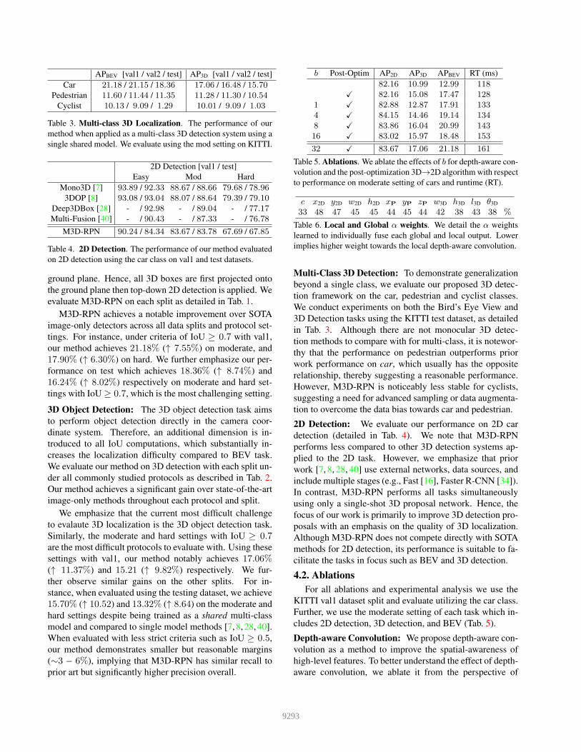
Figure 5. Qualitative Examples. We visualize qualitative examples of our method for multi-class 3D object detection. We use yellow to

denote cars, green for pedestrians, and orange for cyclists. All illustrated images are from the val1 [8] split and not used for training.

the hyperparameter b which denotes the number of discrete

bins. Since our framework uses an image scale of 512 pix-

els with network stride of 16, the output feature map can

naturally be separated into 512

16= 32 bins. We therefore

ablate using bins of [4, 8, 16, 32] as described in Tab. 5.

We additionally ablate the special case of b = 1, which is

the equivalent to utilizing two global streams. We observe

that both b = 1 and b = 4 result in generally worse perfor-

mance than the baseline without local features, suggesting

that arbitrarily adding deeper layers is not inherently help-

ful for 3D localization. However, we observe consistent im-

provements when b = 32 is used, achieving a large gain of

3.71% in APBEV, 1.98% in AP3D, and 1.51% in AP2D.

We breakdown the learned α weights after sigmoid

which are used to fuse the global and local outputs (Tab. 6).

Lower values favor local branch and vice-versa for global.

Interestingly, the classification c output learns the highest

bias toward local features, suggesting that semantic features

in urban scenes have a moderate reliance on depth position.

Post 3D→2D Optimization: The post-optimization algo-

rithm encourages consistency between 3D boxes projected

into the image space and the predicted 2D boxes. We ablate

the effectiveness of this optimization as detailed in Tab. 5.

We observe that the post-optimization has a significant im-

pact on both BEV and 3D detection performance. Specif-

ically, we observe performance gains of 4.48% in APBEV

and 4.09% in AP3D. We additionally observe that the al-

gorithm converges in approximately 8 iterations on average

and adds minor 13 ms overhead (per image) to the runtime.

Efficiency: We emphasize that our approach uses only

a single network for inference and hence involves overall

more direct 3D predictions than the use of multiple net-

works and stages (RPN with R-CNN) used in prior works

[7, 8, 28, 40]. We note that direct efficiency comparison is

difficult due to a lack of reporting in prior work. However,

we comprehensively report the efficiency of M3D-RPN for

each ablation experiment, where b and post-optimization

are the critical factors, as detailed in Tab. 5. The runtime ef-

ficiency is computed using NVIDIA 1080ti GPU averaged

across the KITTI val1 dataset. We note that depth-aware

convolution incurs 2− 20% overhead cost for b = 1 . . . 32,

caused by unfolding and reshaping in PyTorch [30].

5. Conclusion

In this work, we present a reformulation of monocu-

lar image-only 3D object detection using a single-shot 3D

RPN, in contrast to prior work which are comprised of ex-

ternal networks, data sources, and involve multiple stages.

M3D-RPN is uniquely designed with shared 2D and 3D

anchors which leverage strong priors closely linked to the

correlation between 2D scale and 3D depth. To help im-

prove 3D parameter estimation, we further propose depth-

aware convolution layers which enable the network to de-

velop spatially-aware features. Collectively, we are able to

significantly improve the performance on the challenging

KITTI dataset on both the Birds Eye View and 3D object

detection tasks for the car, pedestrian, and cyclist classes.

Acknowledgment: Research was partially sponsored by

the Army Research Office under Grant Number W911NF-

18-1-0330. The views and conclusions contained in this

document are those of the authors and should not be inter-

preted as representing the official policies, either expressed

or implied, of the Army Research Office or the U.S. Gov-

ernment. The U.S. Government is authorized to reproduce

and distribute reprints for Government purposes notwith-

standing any copyright notation herein.

9294

References

[1] Yousef Atoum, Joseph Roth, Michael Bliss, Wende Zhang,

and Xiaoming Liu. Monocular video-based trailer coupler

detection using multiplexer convolutional neural network. In

ICCV. IEEE, 2017. 2

[2] Aseem Behl, Omid Hosseini Jafari, Siva

Karthik Mustikovela, Hassan Abu Alhaija, Carsten Rother,

and Andreas Geiger. Bounding boxes, segmentations and

object coordinates: How important is recognition for 3D

scene flow estimation in autonomous driving scenarios? In

ICCV. IEEE, 2017. 1

[3] Garrick Brazil and Xiaoming Liu. Pedestrian detection with

autoregressive network phases. In CVPR. IEEE, 2019. 2

[4] Garrick Brazil, Xi Yin, and Xiaoming Liu. Illuminating

pedestrians via simultaneous detection segmentation. In

ICCV. IEEE, 2017. 2

[5] Zhaowei Cai, Quanfu Fan, Rogerio S Feris, and Nuno Vas-

concelos. A unified multi-scale deep convolutional neural

network for fast object detection. In ECCV. Springer, 2016.

1, 2

[6] Zhaowei Cai and Nuno Vasconcelos. Cascade R-CNN: Delv-

ing into high quality object detection. In CVPR. IEEE, 2018.

1, 2

[7] Xiaozhi Chen, Kaustav Kundu, Ziyu Zhang, Huimin Ma,

Sanja Fidler, and Raquel Urtasun. Monocular 3D object de-

tection for autonomous driving. In CVPR. IEEE, 2016. 1, 2,

3, 6, 7, 8

[8] Xiaozhi Chen, Kaustav Kundu, Yukun Zhu, Andrew G

Berneshawi, Huimin Ma, Sanja Fidler, and Raquel Urtasun.

3D object proposals for accurate object class detection. In

NIPS, pages 424–432, 2015. 1, 2, 3, 6, 7, 8

[9] Xiaozhi Chen, Huimin Ma, Ji Wan, Bo Li, and Tian Xia.

Multi-view 3D object detection network for autonomous

driving. In CVPR. IEEE, 2017. 2

[10] Yiping Chen, Jingkang Wang, Jonathan Li, Cewu Lu,

Zhipeng Luo, Han Xue, and Cheng Wang. LiDAR-video

driving dataset: Learning driving policies effectively. In

CVPR. IEEE, 2018. 1

[11] Zhe Chen, Shaoli Huang, and Dacheng Tao. Context refine-

ment for object detection. In ECCV. Springer, 2018. 1

[12] Hang Chu, Wei-Chiu Ma, Kaustav Kundu, Raquel Urtasun,

and Sanja Fidler. Surfconv: Bridging 3D and 2D convolution

for RGBD images. In CVPR. IEEE, 2018. 1, 2

[13] Xinxin Du, Marcelo H Ang, Sertac Karaman, and Daniela

Rus. A general pipeline for 3D detection of vehicles. In

ICRA. IEEE, 2018. 2

[14] Mingfei Gao, Ruichi Yu, Ang Li, Vlad I Morariu, and

Larry S Davis. Dynamic zoom-in network for fast object

detection in large images. In CVPR. IEEE, 2018. 1

[15] Andreas Geiger, Philip Lenz, and Raquel Urtasun. Are we

ready for autonomous driving? the KITTI vision benchmark

suite. In CVPR. IEEE, 2012. 1, 2, 3, 6

[16] Ross Girshick. Fast R-CNN. In ICCV. IEEE, 2015. 4, 7

[17] Joris Guerry, Alexandre Boulch, Bertrand Le Saux, Julien

Moras, Aurelien Plyer, and David Filliat. SnapNet-R: Con-

sistent 3D multi-view semantic labeling for robotics. In

ICCV. IEEE, 2017. 1

[18] Gao Huang, Zhuang Liu, Laurens Van Der Maaten, and Kil-

ian Q Weinberger. Densely connected convolutional net-

works. In CVPR. IEEE, 2017. 5

[19] Seung-Wook Kim, Hyong-Keun Kook, Jee-Young Sun,

Mun-Cheon Kang, and Sung-Jea Ko. Parallel feature pyra-

mid network for object detection. In ECCV. Springer, 2018.

1

[20] Tao Kong, Fuchun Sun, Wenbing Huang, and Huaping Liu.

Deep feature pyramid reconfiguration for object detection. In

ECCV. Springer, 2018. 2

[21] Alex Krizhevsky, Ilya Sutskever, and Geoffrey E Hinton.

Imagenet classification with deep convolutional neural net-

works. In NIPS, pages 1097–1105, 2012. 2, 5

[22] Yann LeCun, Patrick Haffner, Leon Bottou, and Yoshua Ben-

gio. Object recognition with gradient-based learning. In

Shape, contour and grouping in computer vision, pages 319–

345. Springer, 1999. 2, 5

[23] Zeming Li, Chao Peng, Gang Yu, Xiangyu Zhang, Yangdong

Deng, and Jian Sun. DetNet: Design backbone for object

detection. In ECCV. Springer, 2018. 2

[24] Ming Liang, Bin Yang, Shenlong Wang, and Raquel Urtasun.

Deep continuous fusion for multi-sensor 3D object detection.

In ECCV. Springer, 2018. 1, 2

[25] Wei Liu, Dragomir Anguelov, Dumitru Erhan, Christian

Szegedy, Scott Reed, Cheng-Yang Fu, and Alexander C

Berg. SSD: Single shot multibox detector. In ECCV.

Springer, 2016. 2

[26] Wei Liu, Shengcai Liao, Weidong Hu, Xuezhi Liang, and

Xiao Chen. Learning efficient single-stage pedestrian detec-

tors by asymptotic localization fitting. In ECCV. Springer,

2018. 2

[27] Xiaoming Liu and Ting Yu. Gradient feature selection for

online boosting. In ICCV. IEEE, 2007. 2

[28] Arsalan Mousavian, Dragomir Anguelov, John Flynn, and

Jana Kosecka. 3D bounding box estimation using deep learn-

ing and geometry. In CVPR. IEEE, 2017. 1, 2, 3, 6, 7, 8

[29] Kemal Oksuz, Baris Can Cam, Emre Akbas, and Sinan

Kalkan. Localization recall precision (LRP): A new perfor-

mance metric for object detection. In ECCV. Springer, 2018.

2

[30] Adam Paszke, Sam Gross, Soumith Chintala, Gregory

Chanan, Edward Yang, Zachary DeVito, Zeming Lin, Al-

ban Desmaison, Luca Antiga, and Adam Lerer. Automatic

differentiation in pytorch. 2017. 5, 6, 8

[31] Charles R Qi, Wei Liu, Chenxia Wu, Hao Su, and Leonidas J

Guibas. Frustum pointnets for 3D object detection from

RGB-D data. In CVPR. IEEE, 2018. 1, 2

[32] Joseph Redmon, Santosh Divvala, Ross Girshick, and Ali

Farhadi. You only look once: Unified, real-time object de-

tection. In CVPR. IEEE, 2016. 2

[33] Jimmy Ren, Xiaohao Chen, Jianbo Liu, Wenxiu Sun, Jiahao

Pang, Qiong Yan, Yu-Wing Tai, and Li Xu. Accurate single

stage detector using recurrent rolling convolution. In CVPR.

IEEE, 2017. 1, 2

[34] Shaoqing Ren, Kaiming He, Ross Girshick, and Jian Sun.

Faster R-CNN: Towards real-time object detection with re-

gion proposal networks. In NIPS, 2015. 2, 3, 4, 7

9295

[35] Shaoshuai Shi, Xiaogang Wang, and Hongsheng Li. PointR-

CNN: 3D object proposal generation and detection from

point cloud. In CVPR. IEEE, 2018. 1, 2

[36] Keisuke Tateno, Federico Tombari, Iro Laina, and Nassir

Navab. CNN-SLAM: Real-time dense monocular slam with

learned depth prediction. In CVPR. IEEE, 2017. 1

[37] Xinlong Wang, Tete Xiao, Yuning Jiang, Shuai Shao, Jian

Sun, and Chunhua Shen. Repulsion loss: Detecting pedestri-

ans in a crowd. In CVPR. IEEE, 2018. 4

[38] Alexander Womg, Mohammad Javad Shafiee, Francis Li,

and Brendan Chwyl. Tiny SSD: A tiny single-shot detection

deep convolutional neural network for real-time embedded

object detection. In CRV. IEEE, 2018. 2

[39] Yu Xiang, Wongun Choi, Yuanqing Lin, and Silvio Savarese.

Subcategory-aware convolutional neural networks for object

proposals and detection. In WACV. IEEE, 2017. 6

[40] Bin Xu and Zhenzhong Chen. Multi-level fusion based 3D

object detection from monocular images. In CVPR. IEEE,

2018. 1, 2, 3, 6, 7, 8

[41] Bin Yang, Wenjie Luo, and Raquel Urtasun. Pixor: Real-

time 3D object detection from point clouds. In CVPR. IEEE,

2018. 1, 2

[42] Fan Yang, Wongun Choi, and Yuanqing Lin. Exploit all the

layers: Fast and accurate CNN object detector with scale de-

pendent pooling and cascaded rejection classifiers. In CVPR.

IEEE, 2016. 2

[43] Jiahui Yu, Yuning Jiang, Zhangyang Wang, Zhimin Cao, and

Thomas Huang. Unitbox: An advanced object detection net-

work. In ICM. ACM, 2016. 4

[44] Zhishuai Zhang, Siyuan Qiao, Cihang Xie, Wei Shen, Bo

Wang, and Alan L Yuille. Single-shot object detection with

enriched semantics. In CVPR. IEEE, 2018. 2

[45] Chunluan Zhou and Junsong Yuan. Bi-box regression for

pedestrian detection and occlusion estimation. In ECCV.

Springer, 2018. 2

9296