M31- Dist of X-bars 1 Department of ISM, University of Alabama, 1992-2003

Sampling Distributions

Our Goal? Our Goal? To make a decisions.To make a decisions.

What are they?

Why do we care?

M31- Dist of X-bars 2 Department of ISM, University of Alabama, 1992-2003

Lesson Objectives

Know what is meant by the “sampling distribution” of a statistic, and the “population of all possible X-bar values.”

Know when the population of allpossible X-bar values IS normal.

Know when the population of allpossible X-bar values IS NOT normal.

M31- Dist of X-bars 3 Department of ISM, University of Alabama, 1992-2003

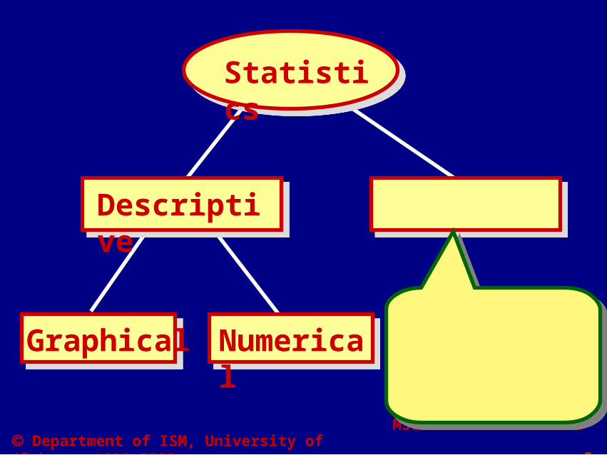
Descriptive

NumericalGraphical

Statistics

M31- Dist of X-bars 4 Department of ISM, University of Alabama, 1992-2003

Statistical Inference

Generalizing from a sample to a population,

by using a statisticto estimate

a parameter.

Goal: Goal: . .

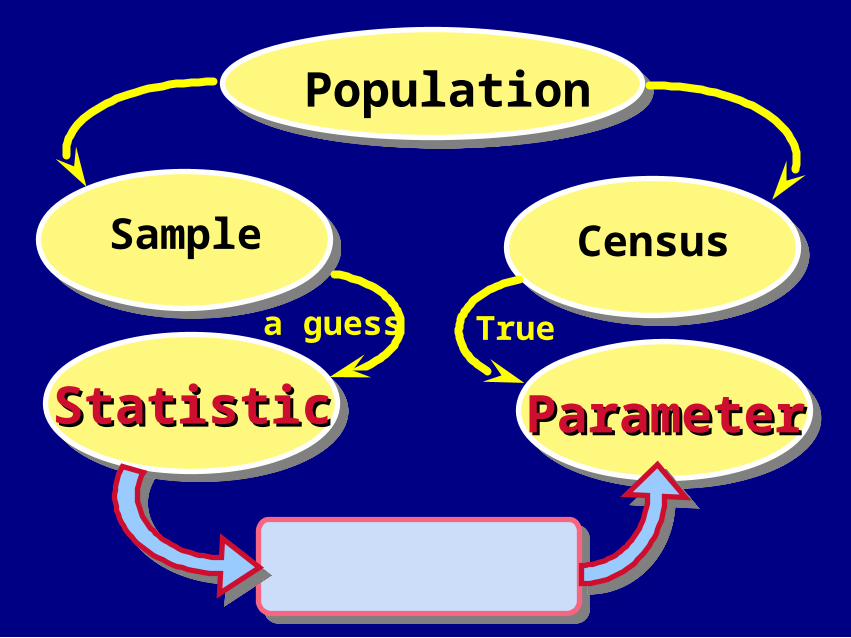
Population

Census

True

ParameterParameter

Sample

StatisticStatistic

a guess

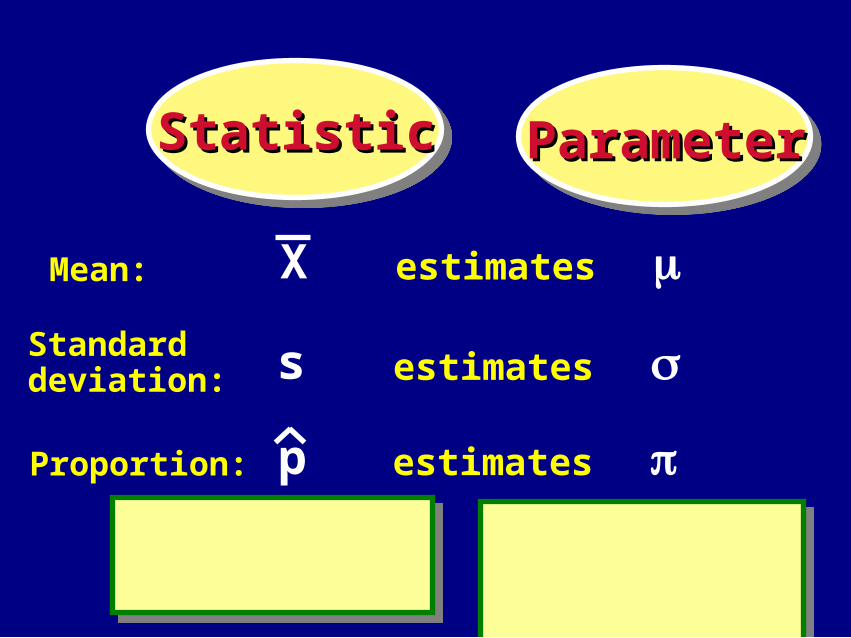
ParameterParameterStatisticStatistic

Mean:

Standard deviation:

Proportion:

s

X

estimates

estimates

estimatesp

M31- Dist of X-bars 7 Department of ISM, University of Alabama, 1992-2003

A A statisticstatistic is a is a . .

Before we can make decisionsBefore we can make decisionsabout parameters about parameters and control and control the degree of riskthe degree of risk, we must know:, we must know:

the the of the statistic of the statistic and its and its values.values.

Objective of this section:

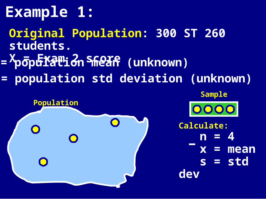
Original Population: 300 ST 260 students.X = Exam 2 score

= population mean (unknown) = population std deviation (unknown)

Calculate:

n = 4 x = mean s = std dev

Example 1:

PopulationSample

M31- Dist of X-bars 9 Department of ISM, University of Alabama, 1992-2003

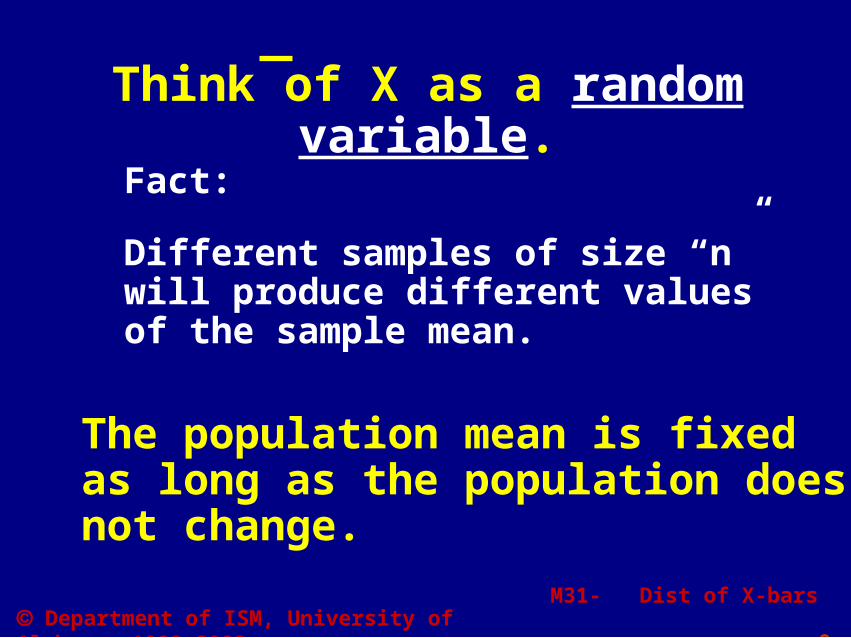
Think of X as a random variable.

Fact:

Different samples of size “n” will produce different values of the sample mean.

The population mean is fixed as long as the population doesnot change.

M31- Dist of X-bars 10 Department of ISM, University of Alabama, 1992-2003

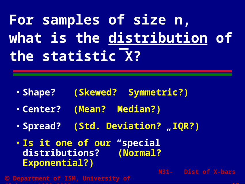
• Shape? (Skewed? Symmetric?)

• Center? (Mean? Median?)

• Spread? (Std. Deviation? IQR?)

• Is it one of our “special” distributions? (Normal? Exponential?)

For samples of size n, what is the distribution of the statistic X?

M31- Dist of X-bars 11 Department of ISM, University of Alabama, 1992-2003

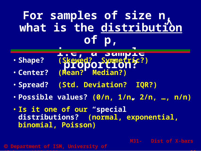
For samples of size n, what is the distribution of p,

i.e, a sample proportion?

• Shape? (Skewed? Symmetric?)

• Center? (Mean? Median?)

• Spread? (Std. Deviation? IQR?)

• Possible values? (0/n, 1/n, 2/n, …, n/n)

• Is it one of our “special” distributions? (normal, exponential, binomial, Poisson)

^

M31- Dist of X-bars 12 Department of ISM, University of Alabama, 1992-2003

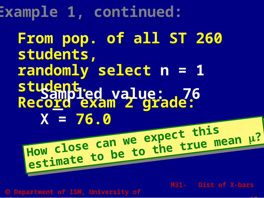
From pop. of all ST 260 students,randomly select n = 1 student.Record exam 2 grade:

Sampled value: 76

X = 76.0

How close can we expect this

estimate to be to the true mean ?How close can we expect this

estimate to be to the true mean ?

Example 1, continued:

M31- Dist of X-bars 13 Department of ISM, University of Alabama, 1992-2003

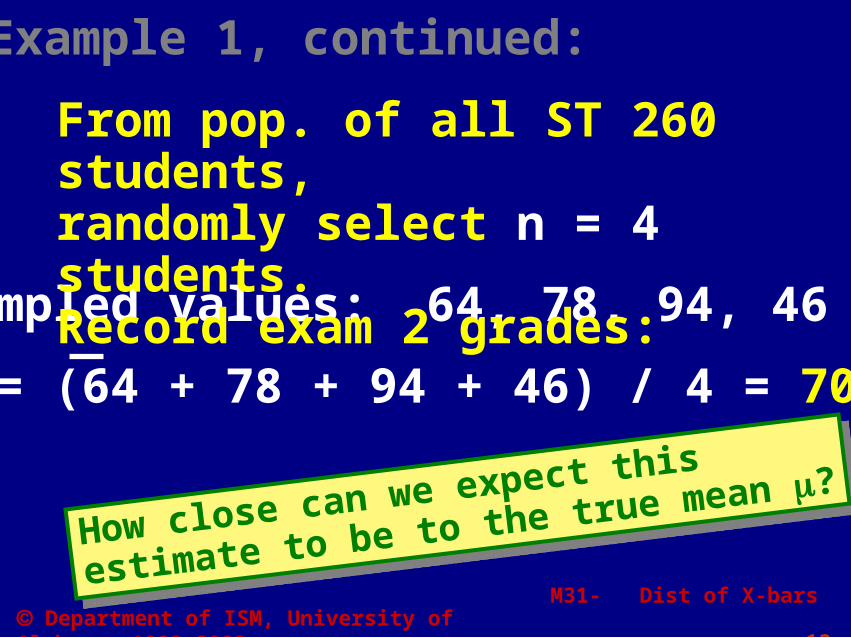
Sampled values: 64, 78, 94, 46

X = (64 + 78 + 94 + 46) / 4 = 70.5

From pop. of all ST 260 students,randomly select n = 4 students.Record exam 2 grades:

How close can we expect this

estimate to be to the true mean ?How close can we expect this

estimate to be to the true mean ?

Example 1, continued:

M31- Dist of X-bars 14 Department of ISM, University of Alabama, 1992-2003

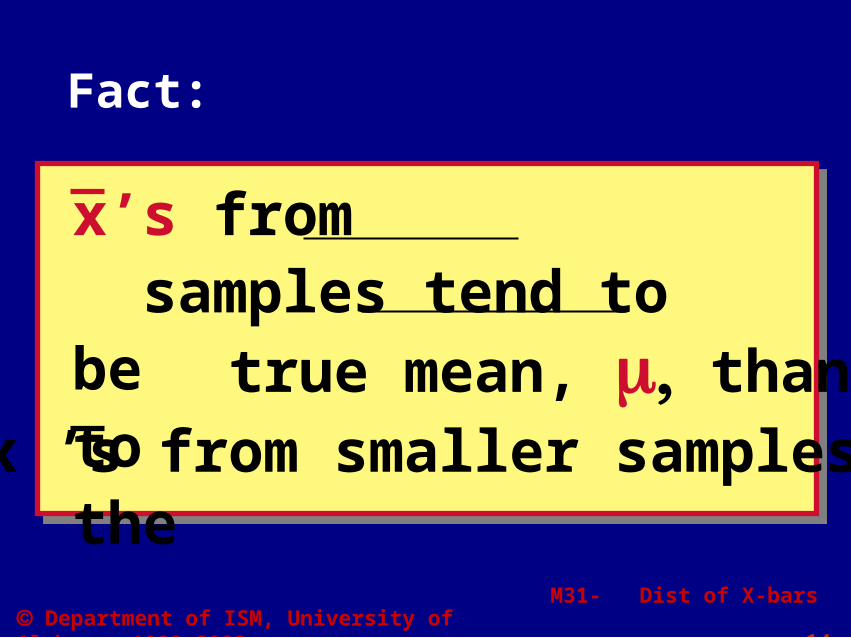
x’s from samples tend to be to the true mean, than x ’s from smaller samples.

Fact:

M31- Dist of X-bars 15 Department of ISM, University of Alabama, 1992-2003

Sampling Distribution of X

is the distribution of all possible

sample means calculated from

all possible samples of size n.

Also calledAlso called “the population “the population

of all possible x-bars”. of all possible x-bars”.

Also calledAlso called “the population “the population

of all possible x-bars”. of all possible x-bars”.

M31- Dist of X-bars 16 Department of ISM, University of Alabama, 1992-2003

And so on, . . . ,

until we collect every possible sample of size n = 4.

How many samples of size 4 are there from a population of 300 members?

M31- Dist of X-bars 17 Department of ISM, University of Alabama, 1992-2003

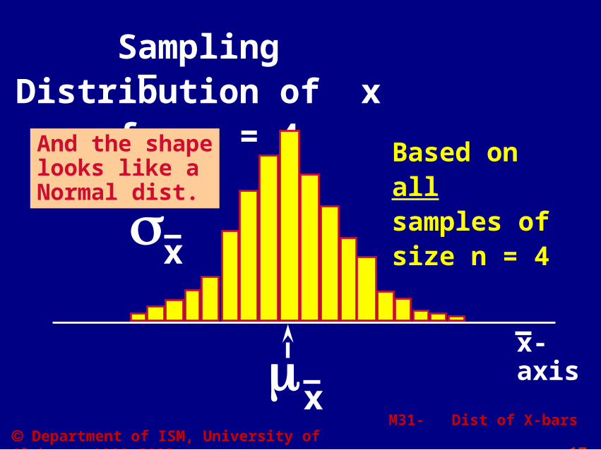
Sampling Distribution of x for n = 4

Based on all samples of size n = 4

x

x

x-axis

And the shapelooks like aNormal dist.

M31- Dist of X-bars 18 Department of ISM, University of Alabama, 1992-2003

x

x

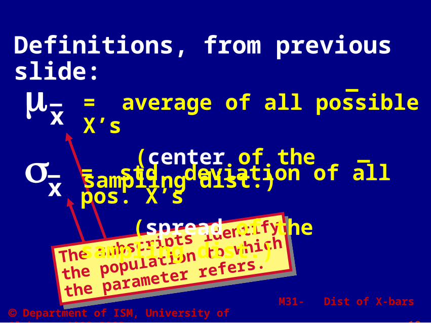
Definitions, from previous slide:

The subscripts identify

the population to which

the parameter refers.The subscripts identify

the population to which

the parameter refers.

= average of all possible X’s

(center of the sampling dist.)

= std. deviation of all pos. X’s

(spread of the sampling dist.)

M31- Dist of X-bars 19 Department of ISM, University of Alabama, 1992-2003

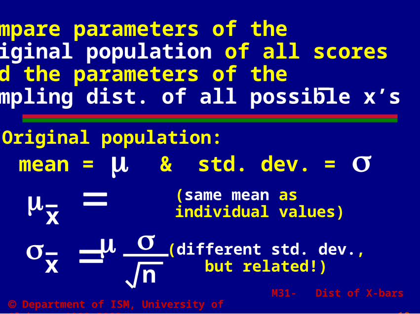
Compare parameters of theoriginal population of all scores and the parameters of the sampling dist. of all possible x’s

mean = & std. dev. = Original population:

x

x

(same mean as individual values)

n

(different std. dev., but related!)

M31- Dist of X-bars 20 Department of ISM, University of Alabama, 1992-2003

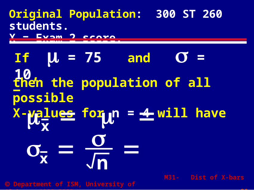
If = 75 and = 10,

Original Population: 300 ST 260 students.X = Exam 2 score.

then the population of all possible X-values for n = 4 will have

x

x n

M31- Dist of X-bars 21 Department of ISM, University of Alabama, 1992-2003

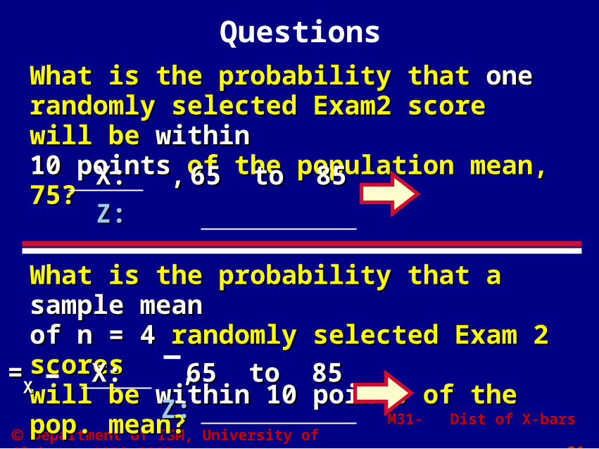
Questions

What is the probability that What is the probability that oneone randomly randomly selected Exam2 score will be selected Exam2 score will be within within 10 points10 points of the population mean, 75? of the population mean, 75?

X: 65 to 85X: 65 to 85

Z:Z:

= ,= ,

What is the probability that a What is the probability that a sample mean sample mean of n = 4of n = 4 randomly selected Exam 2 scores randomly selected Exam 2 scores will be will be within 10 pointswithin 10 points of the pop. mean? of the pop. mean?

= ,= ,XX

X: 65 to 85 X: 65 to 85

Z:Z:

M31- Dist of X-bars 23 Department of ISM, University of Alabama, 1992-2003

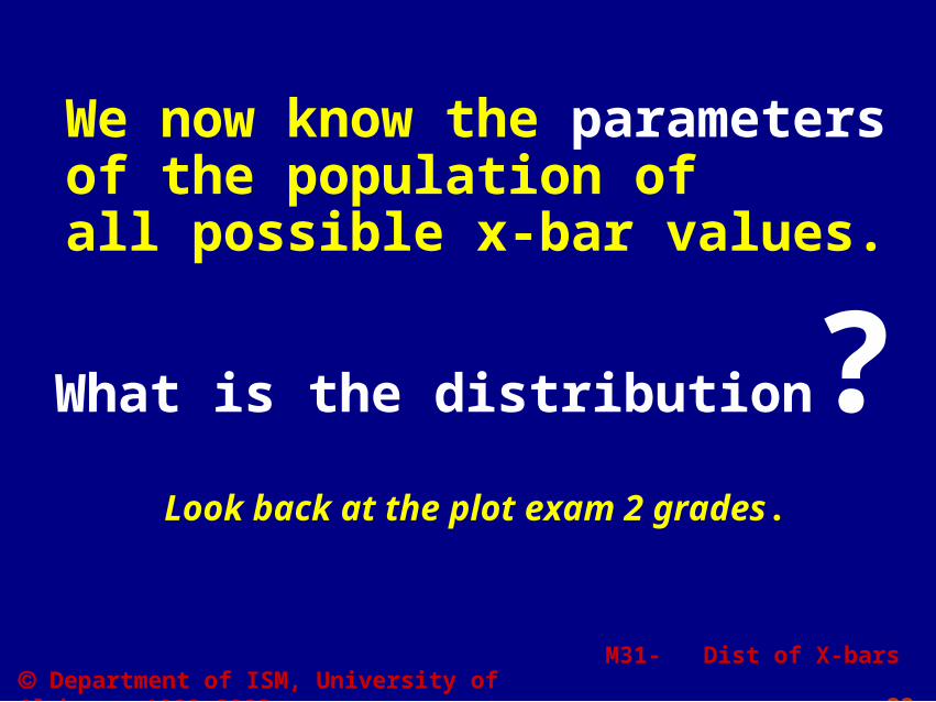
We now know the parametersof the population of all possible x-bar values.

What is the distribution?Look back at the plot exam 2 grades.

M31- Dist of X-bars 24 Department of ISM, University of Alabama, 1992-2003

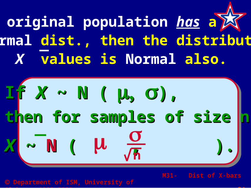
If If XX ~ N ( ~ N ( ),),

then for samples of size n,then for samples of size n,

XX ~ ~ NN ( ( ,, ). ).

If original population has aNormal dist., then the distributionof X values is Normal also.

n

M31- Dist of X-bars 25 Department of ISM, University of Alabama, 1992-2003

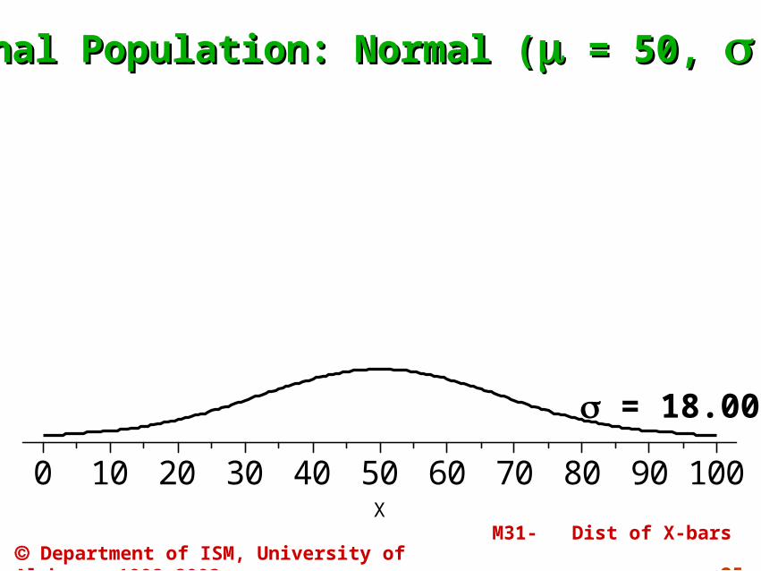
1009080706050403020100X

Original PopulationOriginal Population: Normal (: Normal ( = 50, = 50, = 18) = 18)

= 18.00

M31- Dist of X-bars 26 Department of ISM, University of Alabama, 1992-2003

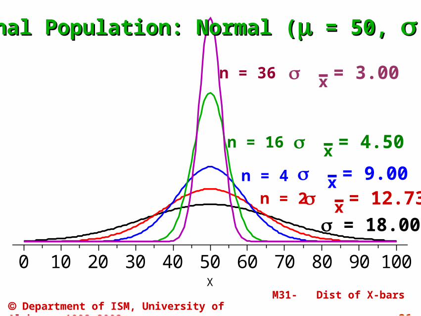
1009080706050403020100X

Original PopulationOriginal Population: Normal (: Normal ( = 50, = 50, = 18) = 18)

n = 36

n = 16

n = 4

n = 2

= 9.00x = 12.73x

= 4.50x

= 3.00x

= 18.00

M31- Dist of X-bars 27 Department of ISM, University of Alabama, 1992-2003

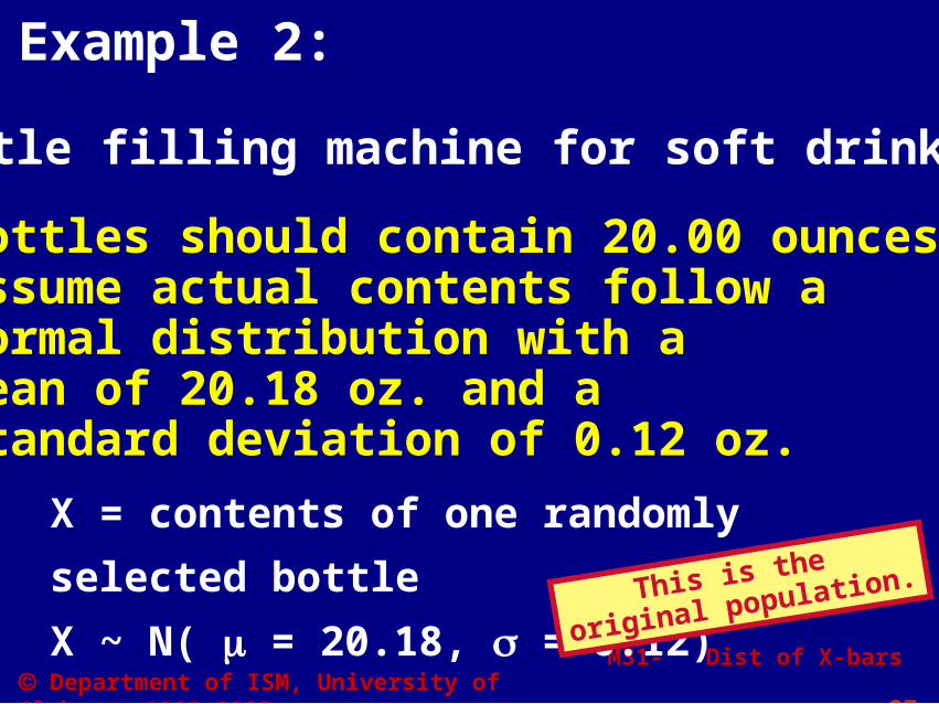
Bottle filling machine for soft drink.

Bottles should contain 20.00 ounces;assume actual contents follow a normal distribution with a mean of 20.18 oz. and a standard deviation of 0.12 oz.

X = contents of one randomly selected bottle

X ~ N( = 20.18, = 0.12)

Example 2:

This is the

original population.

M31- Dist of X-bars 28 Department of ISM, University of Alabama, 1992-2003

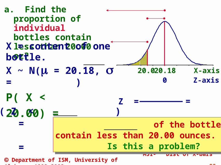
P( X < 20.00)

=

-4.0 -3.0 -2.0 -1.0 0.0 1.0 2.0 3.0 4.0

0

= P( Z < )

a. Find the proportion of individual bottles contain less than 20.00 oz?

20.1820.0

Z =

X = content of one bottle.X ~ N( = 20.18, = )

of the bottles will contain less than 20.00 ounces. Is this a problem?

of the bottles will contain less than 20.00 ounces. Is this a problem?

=

Z-axisX-axis

=

=

M31- Dist of X-bars 29 Department of ISM, University of Alabama, 1992-2003

-4.0 -3.0 -2.0 -1.0 0.0 1.0 2.0 3.0 4.0

0

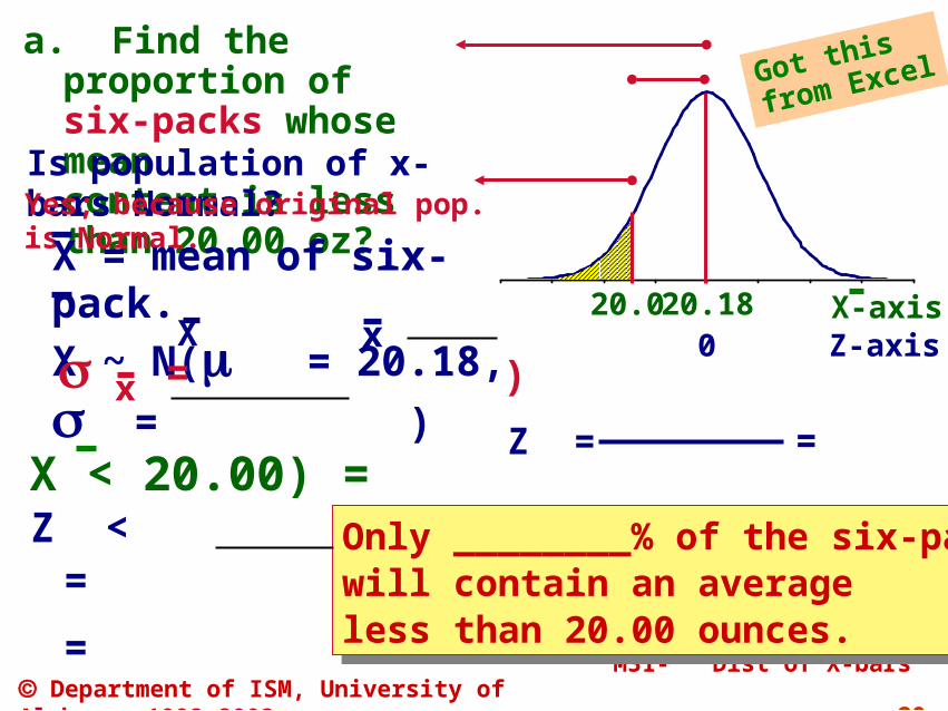
= P( Z < )

a. Find the proportion of six-packs whose mean content is less than 20.00 oz?

20.1820.0

Z =

Only ________% of the six-packswill contain an average less than 20.00 ounces.

Only ________% of the six-packswill contain an average less than 20.00 ounces.

=

Z-axisX-axis

=

=

Is population of x-bars Normal?Yes; because original pop. is Normal.

X = mean of six-pack.X ~ N( = 20.18, = )X x

x = )

P( X < 20.00) =

Got this

from Excel

M31- Dist of X-bars 30 Department of ISM, University of Alabama, 1992-2003

M31- Dist of X-bars 31 Department of ISM, University of Alabama, 1992-2003

New situation

Such as an . . .

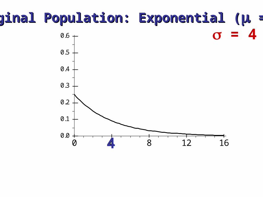
Exponential Distribution?Such as an . . .

Exponential Distribution?

But what if the original population

is not normally distributed?

M31- Dist of X-bars 32 Department of ISM, University of Alabama, 1992-2003

Demonstration Demonstration of theof the

Central Limit TheoremCentral Limit Theorem

Page 289

1612840

0.6

0.5

0.4

0.3

0.2

0.1

0.0

Original Population: Exponential (Original Population: Exponential ( = 4) = 4)

n = 1

= 4

4

1612840

0.6

0.5

0.4

0.3

0.2

0.1

0.0

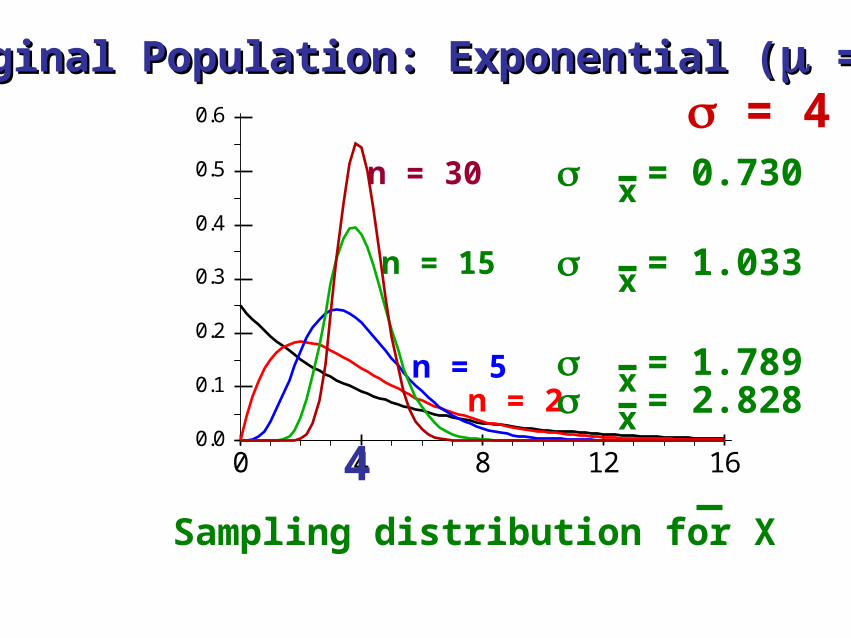
Original Population: Exponential (Original Population: Exponential ( = 4) = 4)

n = 30

n = 15

n = 5n = 2

= 4

Sampling distribution for X

= 1.789x = 2.828x

= 1.033x

= 0.730x

4

M31- Dist of X-bars 35 Department of ISM, University of Alabama, 1992-2003

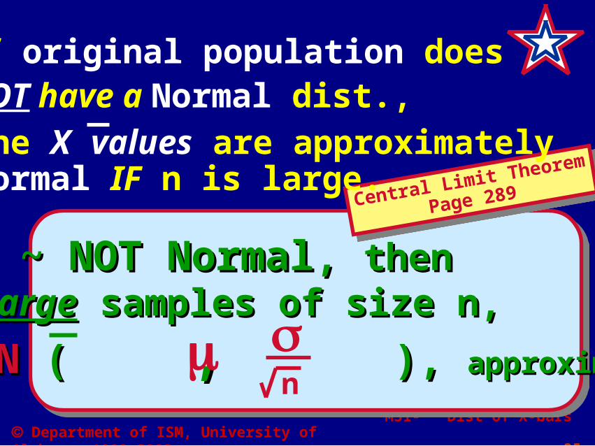
If If XX ~ NOT Normal, ~ NOT Normal, then then for for largelarge samples of size n, samples of size n,

XX ~ ~ NN ( ( ,, ), ), approximately.approximately.

If original population doesNOT have a Normal dist.,

n

Central Limit Theorem

Page 289Central Limit Theorem

Page 289

the X values are approximately Normal IF n is large.

M31- Dist of X-bars 36 Department of ISM, University of Alabama, 1992-2003

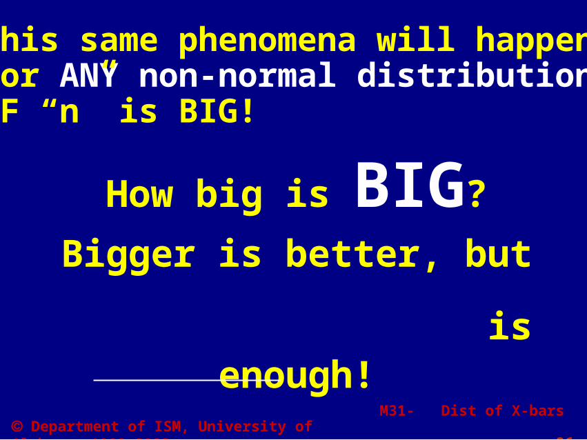
How big is BIG?

Bigger is better, but

is enough!

This same phenomena will happenfor ANY non-normal distribution,IF “n” is BIG!

M31- Dist of X-bars 37 Department of ISM, University of Alabama, 1992-2003

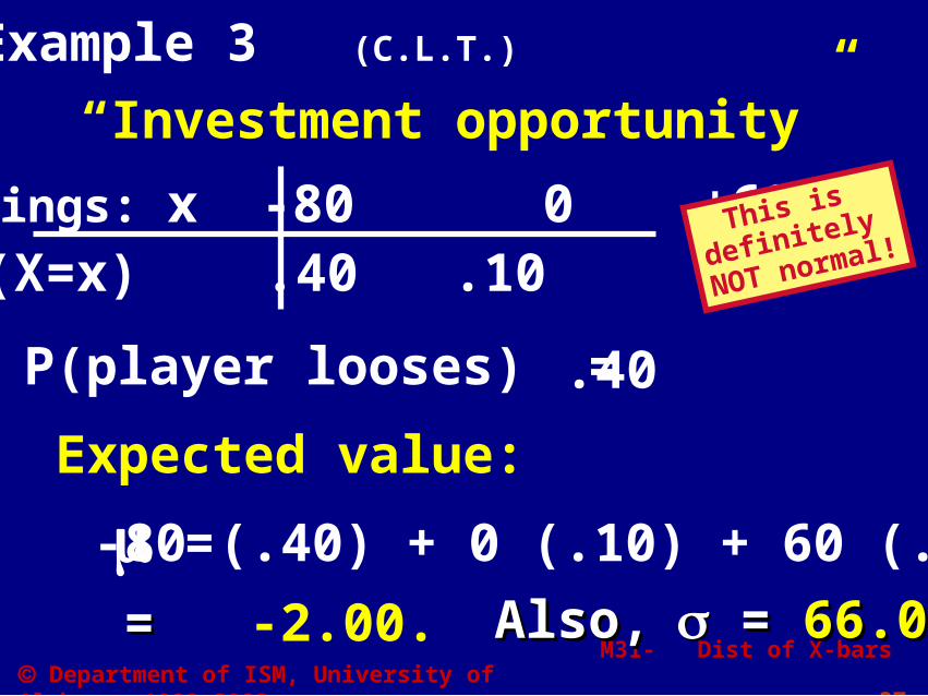
“Investment opportunity”

Earnings: x -80 0 +60 P(X=x) .40 .10 .50

P(player looses) = .40

Expected value:

= -80 (.40) + 0 (.10) + 60 (.50)

Also,Also, = = 66.066.0= = -2.00.

Example 3 (C.L.T.)

This is

definitely

NOT normal!

M31- Dist of X-bars 38 Department of ISM, University of Alabama, 1992-2003

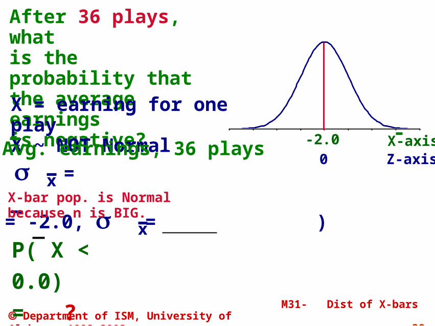
P( X < 0.0) = ?

-4.0 -3.0 -2.0 -1.0 0.0 1.0 2.0 3.0 4.0

0 Z-axis

After 36 plays, what is the probability that the average earnings is negative?

-2.0

X = earning for one playX ~ NOT Normal

= x

X ~ N( = -2.0, = )x

X = Avg. earnings, 36 plays X-axis

X-bar pop. is Normal because n is BIG.

M31- Dist of X-bars 39 Department of ISM, University of Alabama, 1992-2003

-4.0 -3.0 -2.0 -1.0 0.0 1.0 2.0 3.0 4.0

Z-axis

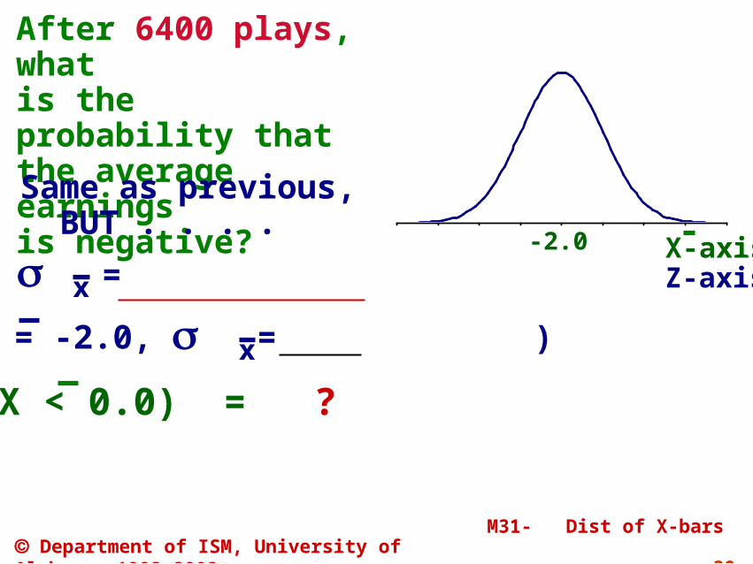
After 6400 plays, what

is the probability that the average earnings is negative?

-2.0

Same as previous, BUT . . . .

= x

X ~ N( = -2.0, = )x

X-axis

P( X < 0.0) = ?

M31- Dist of X-bars 40 Department of ISM, University of Alabama, 1992-2003

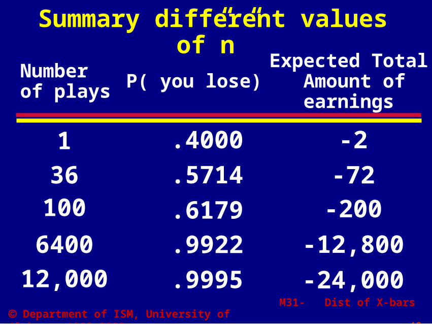
Summary different values of”n”

Number of plays P( you lose)

Expected Total Amount ofearnings

1 .4000 -2

36 .5714 -72100 .6179 -200

6400 .9922 -12,800

12,000 .9995 -24,000

M31- Dist of X-bars 41 Department of ISM, University of Alabama, 1992-2003

The house never

The house never

loses!loses!The house never

The house never

loses!loses!

M31- Dist of X-bars 42 Department of ISM, University of Alabama, 1992-2003

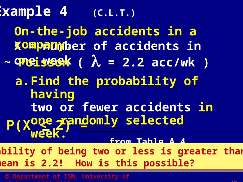
X = number of accidents in one week

On-the-job accidents in a company.

X ~ Poisson ( = 2.2 acc/wk )

Example 4 (C.L.T.)

a. Find the probability of having two or fewer accidents in one randomly selected week.

P(X < 2) = , from Table A.4. This is a Chapter 6 problem.

The probability of being two or less is greater than .5, but the mean is 2.2! How is this possible?

The probability of being two or less is greater than .5, but the mean is 2.2! How is this possible?

M31- Dist of X-bars 43 Department of ISM, University of Alabama, 1992-2003

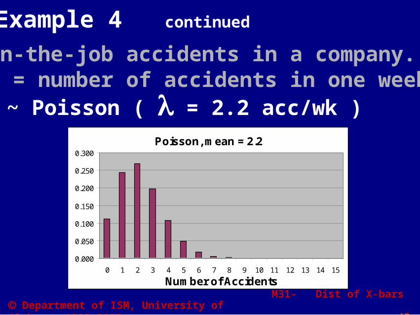
Example 4 continued

X = number of accidents in one weekOn-the-job accidents in a company.

X ~ Poisson ( = 2.2 acc/wk )Poisson, mean = 2.2

0.000

0.050

0.100

0.150

0.200

0.250

0.300

0 1 2 3 4 5 6 7 8 9 10 11 12 13 14 15

Number of Accidents

M31- Dist of X-bars 44 Department of ISM, University of Alabama, 1992-2003

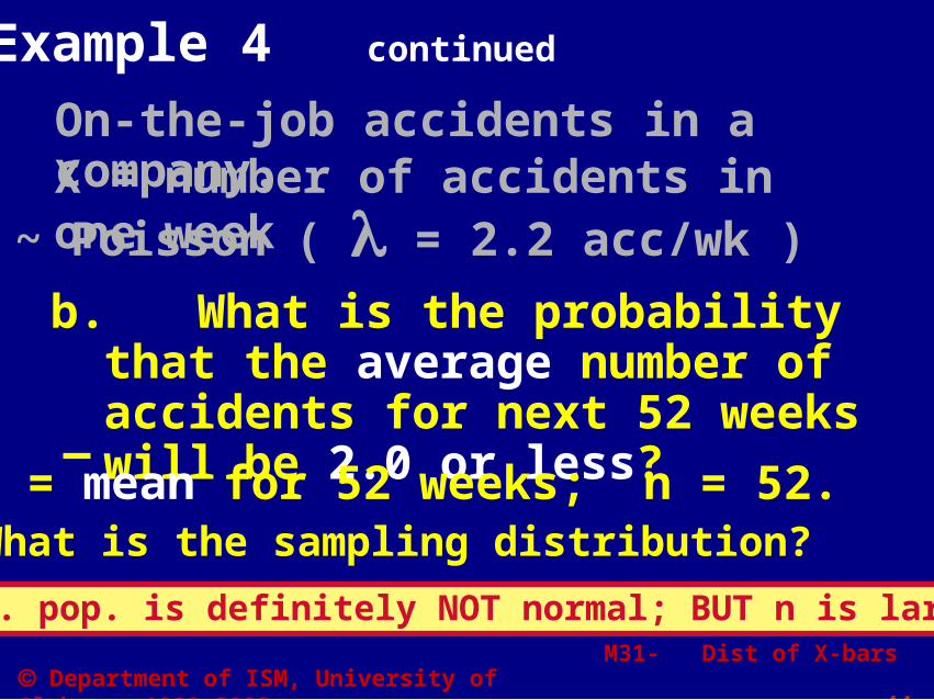
Example 4 continued

Ori. pop. is definitely NOT normal; BUT n is large!

b. What is the probability that the average number of accidents for next 52 weeks will be 2.0 or less?

X = mean for 52 weeks; n = 52.What is the sampling distribution?

X = number of accidents in one week

On-the-job accidents in a company.

X ~ Poisson ( = 2.2 acc/wk )

M31- Dist of X-bars 45 Department of ISM, University of Alabama, 1992-2003

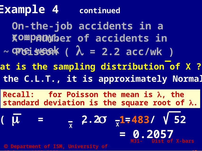
What is the sampling distribution of X ?

XXX ~ N ( = , = )2.2 1.483/ 52

By the C.L.T., it is approximately Normal.

Recall: for Poisson the mean is , the standard deviation is the square root of .

= 0.2057

Example 4 continued

X = number of accidents in one week

On-the-job accidents in a company.

X ~ Poisson ( = 2.2 acc/wk )

M31- Dist of X-bars 46 Department of ISM, University of Alabama, 1992-2003

-4.0 -3.0 -2.0 -1.0 0.0 1.0 2.0 3.0 4.0

0

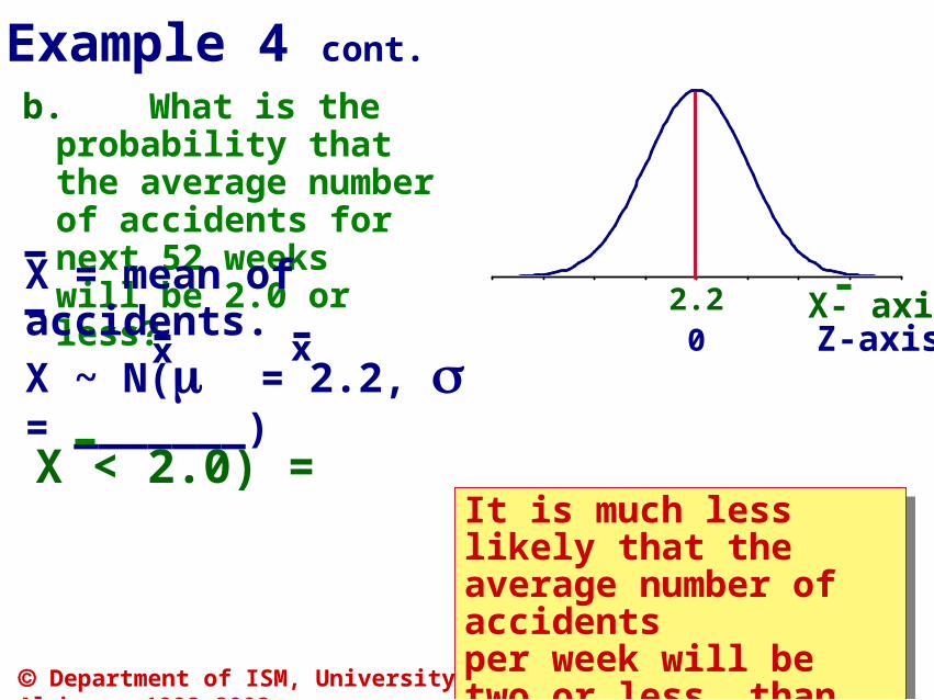
b. What is the probability that the average number of accidents for next 52 weeks

will be 2.0 or less? 2.2

It is much less likely that the average number of accidents per week will be two or less, than any one specific week.

It is much less likely that the average number of accidents per week will be two or less, than any one specific week.

Z-axisX- axis

X = mean of accidents.X ~ N( = 2.2, = _______)x x

P( X < 2.0) =

Example 4 cont.

M31- Dist of X-bars 47 Department of ISM, University of Alabama, 1992-2003

Anytime the original pop. is Normal (true for any n).

Anytime the original pop. is not Normal, but n is BIG (n > 30).

Reminder

When is the population of all possible X values Normal?

M31- Dist of X-bars 48 Department of ISM, University of Alabama, 1992-2003

Anytime the original population

is not Normal AND

n is NOT BIG.

Remember

When is the population of all possible X values NOT Normal?