t .'

T/YI- 8//42

Atmospheric Particulate Analysis Using

Angular light Scattering

M. Z. Hansen

(NASA-TH-81112) ATMOSPHERIC PARTICULATEANALYSIS USING ANGULAR LxvHT SCATTERING

N8J-31995(NASA) 40 p HC A03/bF A01 CSCL 04A

UnclasG3/46 32513

Submitted to Applied Optics

cz.)4 E,V Ep _

`^ ESS DEpj ^'

The majority of this work was completed while the author was at theUniversity of Arizona, Institute of Atmospheric Physics, Tucson, $5721.'The author is presently with the Goddard Space Flight Center, Laboratoryfor Atmospheric Sciences, Greenbelt, Maryland 20771.

https://ntrs.nasa.gov/search.jsp?R=19800023488 2018-06-12T22:00:30+00:00Z

Using the light scattering matrix elements measured by a polar

nephelometer, a procedure for estimating the characteristics of

atmospheric particulates was developed. A theoretical library data

set of scattering matrices derived from Me theory was tabulated for

a range of values of the size parameter and refractive index typical

of atmospheric particles. integration over the size parameter yielded

the scattering matrix elements for a variety of hypothesized particu-

late size distributions. A least squares curve fitting technique was

used to find a best fit from the library data for the experimental

measurements. This was used as a first guess for a nonlinear iterative

Inversion of the size distributions. A real index of 1.50 and an

Imaginary index of -0.005 are representative of the smoothed inversion

results for the near ground level atmospheric aerosol in Tucson.

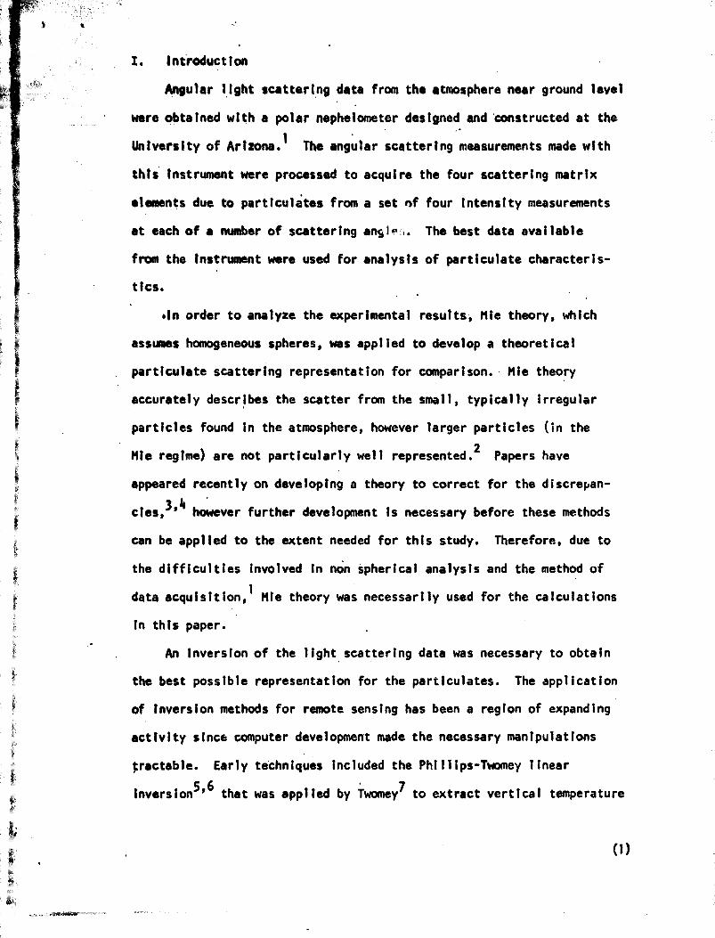
L Introduction

Angular light scattering data from the atmosphere near ground level

were obtained with a polar nephelometer designed and'constructed at the

University of Arizona. ) The angular scattering measurements made with

this instrument were processed to acquire the four scattering matrix

elements due to particulates from a set of four intensity measurements

at each of a number of scattering ang1P::. The best data available

from the instrument were used for analysis of particulate characteris-

tics.

,In order to analyze the experimental results, Hie theory, which

assumes homogeneous spheres, was applied to develop a theoretical

particulate scattering representation for comparison. Hie theory

accurately describes the scatter from the small, typically irregular

particles found in the atmosphere, however larger particles (in the

Hie regime) are not particularly well represented. 2 Papers have

appeared recently on developing a theory to correct for the discrepan-

cies,3 ' 4 however further development is necessary before these methods

can be applied to the extent needed for this study. Therefore, due to

the difficulties involved in non spherical analysis and the method of

data acquisition, ) Hie theory was necessarily used for the calculations

in this paper.

An inversion of the light scattering data was necessary to obtain

the best possible representation for the particulates. The application

of inversion methods for remote sensing has been a region of expanding

activity since computer development made the necessary manipulations

tractable. Early techniques included the Phillips-Twomey linear

inversion5

' 6 that was applied by Twomey) to extract vertical temperature

(1)

profiles in the atmosphere. This linear method has been used extensively,

with success in the analysis of atmospheric particulates from multiwave-

length extinction data,$

i The inversion of atmospheric aerosol angular scattering data to

obtain particulate information has typically met with only marginal

success. .Wastwater and Cohen 10 felt that the Backus-Gilbert inversion'

could retrieve size distributions with angular scattering data from

their theoretical study'with multiwavelength scattering. Postll applied

this method to multiple angle scattering measurements from vaster droplets,

but had poor results at sizes below 10um in radius. Both Post and

Vestwater and Cohen used narrow size distributions and still had a

deterioration of results at small sizes. Some success has been achieved

In inverting bistatic lidar data of atmospheric particulates 12

with the

linear method, but only a very limited data set was available.13

The reasons for using one inversion scheme over another are almost

as varied as the investigators, however the nonlinear algorithm technique

of Twomey 14

has shown promise in retrieving particulate size distribu-

tions and was chosen on this basis for application to angular scattering

measurements in this paper.

II. Data Evaluation Method

An estimate of the size distribution and refractive index of an

atmospheric sample is made by comparing the four scattering matrix

elements measured at various angles with the nephelometer with element`

produced by theoretical.size distributions for various indices of

refraction. A library data set on magnetic tape was created using a

(2)

subroutine by Daveis for scattering by a sphere. Matrix elements were

recorded for 500 size paraoters 10.3 (0.2)100.13 at every integral angle

10°01180°1 of scatter for all combinations of a set of real indices of

refraction 11.40, 1.45, 1.50, 1.54, i.601 and imaginary Indices of refrac-

tion 10.0, -0.003, -0.005, -0.01, -0,'031. (Size parameter, a, is 211

times the particle radius divided by the wavelength of incident light,

0.5145 Vm i'n this case.) The range of real indices was chosen to encom-

pass a region from near that of water up past that for silicates. The

Imaginary index values vary from ho absorption as for water to a value

of -0.03 which is near what King 16

has observed.

Subsequently, these data are integrated over the size parameters

for Junge and two-slope size distributions (Figs. 1-3). The Junge*

size distributions are calculated by setting

dN = Cr- (v+i )

(1)

where N is the partici p number concentration, r is the particle radius,

C is a normalization value set to give 100 uglm 3 mass loading, and v

varies, over a typical range from 2.0 to 4.0-in 0.2 steps. The two-slope

'size distributions are calculated by setting

dN ( i + (rlrB)v2)

= C (1 + (r/rd'O"

(2)

where all combinations of rA = 0.04 um, rg = 0.4 and '1.0 um, v l = 2.09

3.0, and 4.0, and vx = 0.0, 1.0, and 1.5 are used. These parameters

were chosen to give turnover values between 0.01 and 0.1 um. These are

above the values observed by Twomey $ 17 but a higher turnover point is

necessary if any effect were to be observed on the scattering data.

(3)

Comparisons are made between these size distributions and real

data by allowing the mass loading to vary to give a best least squares

fit. The quality of the fit is determined by the size of H, given byH'a Z {b i - Cd l ) 2 (3)

12

where 9 is evaluated at Zd ib I d i for a minimum H and functions as a

mass loadtng.adjustment to obtain the best fit. b i is the observed aerosol

scattering matrix element, and d i is the corresponding theoretical

matrix element normalized for lOd uglm 3 . Biasing of the data according

to scattering volume is also used. Outside the range of the size

parameters on tape, the number concentrations are inadequate (for any

realistic size distribution and visible'waveiengths of light) to affect

the observed scatter and are neglected. The tabulated comparisons are

evaluated to find the best least squares fit with-reasonable mass loading

and to observe any .tendencies such as sensitivity to the parameters that

are varied.

Due to the similarity of many of the kernels, little information

Is gained by using a complete range of angles to obtain a size distribu-

tion. The additional time involved in making excessive measurements can

also be detrimental due to possible changes in the sampled aerosol.

Therefore, consideration should be given to which angles are most

critical. Angles where the scattered light i; minimal have more error

and should be avoided. Also, angles where the scattered radiance changes

very quickly are affected more by positioning error in the detector.

By considering angular scattering measurements made on monodisperse

particles, 2 one finds that . for larger nonspherical laboratory aerosols,

tk)

j [

Hie theory saws to hold best for angles less than about 44 degrees.

Smaller aerosols (as they approach the Raylei gh regime) tend to-follow

his theory quite well. This leads one to Inspect where the larger

aerosols contribute to the scatter. By looking at Figs. 4 and 5, one

observes that the difference due to the large aerosols is limited

mainly to the forward few'degrees. This not only implies that Mie theory

should hold better for a typical aerosol size distribution than for

single large aerosol studies, but that if one desires information con-

tent from the larger aerosols, measurements must be made 'in the forward

direction or little information above i um is obtained for typical size

distributions.

III. Inversion Technique

Continuing with the next step, the Inversion method is considered.

A nonlinear algorithm was developed by Chahine l$ which essentially

assumed delta functions for kernels but acquired inherent instabilities

due to Increased high frequency content when measurements were numerous.

Chahine's algorithm was modified by Twomey 14

to include the entire

nonzero region of the kernel. This eliminated the detrimental factor of

superfluous data and, in fact, caused the Inversion to improve with

additional data due to an effective decrease in measurement error.

The nonlinear inversion has also shown an ability to cope with measure-

ment errors, which greatly strengthens its position in application to

the aerosol size distribution problem. The iterative algorithm is

(5)

i

f' (r) •^ l+s _ 1 k r sfgtr)

(4)f (r)k(r,$)dr k(s)max

where f (r) is the initial guess size distribution, k(r,$) is the kernel

value (the theoretical scattering matrix element for a single particle),

g(s) is the actual measured scattering matrix element for the collection

of particiss, and f l (r) is the modified size distribution. Variable r

refers to the particle radius or size parameter, and variable s refers

to a specific matrix element measurement. Examination of the kernels

shows that a lot of fine structure . typically occurs (Figs. 6-9), particu-

larly near backscatter. Whereas this might be expected to be beneficial

for fine resolution, in practice this structure is too high a frequency to

be effective in improving the inversion accuracy. Since atmospheric aero-

sol size distributions do not seen to have these wild oscillations and

neither do the observed scattering measurements, the fine structure would

not seem necessary to resolve that data even if it were effectively usable.

In fact, it might be desirable to use smoothing of the kernel to assist in

obtaining a stable solution. The power spectra of the kernels also show

that the middle frequencies are often deficient (Fig. 10), and occasionally

even low frequencies are absent (Fig. 11). This is a strong negative factor

in the application of scattering kernels to inversion techniques.

Simple quadrature is used for the integral with the kernels being

read from magnetic tape. Each data value is successively iterated once

through all'the particle sizes on tape, modifying the size distribution

according to the kernel's weighting effect. The weighting is scaled to

less than or equal to one by dividing by the maximum kernel value for a

particular angle and matrix element. After each unknown in the set has

been determined from the first iteration, the process is repeated until

(6)

Is obtained. Although the inversion lends itselfthe final distribution

easily to programming, care is still required In its application.

IV. Inversion of Theoretical Data

Initial runs of the Inversion program were made on data generated

from Mie theory to establish the accuracy of the Inversion with scattering

kernels. The nephelometer measures the radiance of light scatter which

is a function of the particles' scattering cross sections times their

concentrations. It was necessary to weight the scattering kernels

according to an initial, first guess size distribution to obtain reasonable

results. Otherwise, there was a strong tendency for the inversion to

adjust the large particle concentrations to the point of instability.

The runs were made using only the M2 and M 1 elements 1from five forward

angles and two backward angles. These were chosen to maximize Information

content with a minimum of data. A special problem occurs in applying

inversions to the S 21 and D21 elements as it is possible for the theoreti-

cal and measured values to be of opposite sign due to errors in the

measurements or in the first guess size distribution. This would imply

a negative particle concentration that is not allowed. Runs were made

with theoretical data from Junge distributions. A v of two, index of

1.54'- .0051, and mass loadlog of 38 ug/m 3 were used for a first guess,

as these values produced a close fit for one of the real aerosol runs.

A method of overrelaxation was settled upon as the best technique for

applying the algorithm. it has the format

f' (r) - {1 + MR} fo(r) (5)

(7)

where

Ms i k; s

f (r)k(r,$)dr _ max

The absolute value of M is raised to the power R, and that quantity takes

the same positive or negative sign as M.

Not only did overrelaxation with values of R less then one speed

up convergence, but It improved the results grestly (Fig. 12). Too large

of an overrelaxation, however, caused oscillations. A value of 1.7 for R

produced the best stability and convergence although 0.5 gave the fastest

convergence. Excessive iterations are not only costly, but tend to pro-

duce a more highly structured, atypical size distribution. This is

avoided by terminating the iterative process after successive iterations

with less than 0.2 percent improvement in error.

The Inversion program was run with theoretical data to observe the

effect of various size distribution first guesses on the results of the

inversion. large differences between the actual and initial guess mass

loading were difficult for the inversion to handle If no internal mass

loading adjustment is included in the program (Fig. 13). This serves

to point out graphically the size range of information content of the

data and the kind of structure'that can occur due to the oscillatory

nature of the kernels. The response in the region of information

content is adequate to indicate the proper correction necessary (i.e.

higher or lower) in the mass loading. Differences between the actual

and initial guess v values (Fig. 14) have much less effect on the

Inversion. Examination of the region of convergence does show that the

.

.r

scattering Is mainly sensitive to particles In the 0.2 to 2 Um range

and subsequently, this is the region where results are applicable.

Random error was added to the theoretical data to observe Its

effect on the inversion. Neither 4 nor it percent error had a signifi-

cant effect on the Inverted size distribution. This result is essential

to obtaining realistic inversions with experimental data. The convergence

limit on the error (fig. 15) %es, In fact, indicative of the percentage

error in the data; however, more study of this point Is necessary for

verification.

The linear inversion method was also applied to this problem initially.

However, it could not invert the data unless the error level was I percent

or less. This Is an unrealistically low value, especially since Mie theory

alone can account for more than 1 parcent'error. Therefore, the linear

method was dropped.

V. Experimental Results

After checking the ability of the Inversion to reproduce theoretical

data, experimental data were analysed.

A. Curve i'itting

By comparing the experimental data with the theoretical library

data, a best fit was obtained. Typically, about 20 scattering angles

with four matrix elements at each angle were used. The fit was weighted

by the cosecant of the scattering angle to allow more bias for larger

scattering volumes. After checking the data fit with matrix elements

produced by both Jung* and two-slope size distributions and using trun-

cated data sets that excluded measurements of smaller magnitude, an

^9)

estimate for the aerosol srze distribution was obtained. The nephelometer

runs for Harch 9th were averaged and gave a Junge bust fit with3

• - 1.50 - .0031, v • 2.1. and mass loading - 38 bag/m . The two-slope

best fit for the same data was m * 1.50 - .0031, vt - 2.0. v2 - 0,

rA - .04 isa, rg n 1.0 pm. and mass loading - 80 leg /m3.

The mass loading is not extremely critical as the largest particies

dominate this value while they have much less effect on the actual

light scatter on which the measurements are based. Another set of

runs on March 10th was averaged to yield a Junge best fit with3

m - 1.47 - .0091, v - 2.0,^and mass loading - 47 Win 'and two-slope 'it

with m - 1.50 - .0041, v i - 2.0, v2 - 0 . 0, r - .04 lum, rg u 1.0 wa,

and mass loading - 1011 pg/m3 . figs. 16 " 17 show typical graphs of

the experimentally measured matrix elements plotted in comparison with

the theoretical data produced by the corresponding best fit size distribu-

tion. As expected, the curves match closeiy near the forward direction

which is where Mis theory is believed to hold best and where the strongest

welvhting is placed on the least squares fit. The two-slope tnd Junge

distributions which gave the best fits are of similar form over the size

range of information content. Therefore, the siopler Junge distribution

was chosen for combining the March data which gave an overall aerosol3

characterization of m - 1.49 - .0041. v - 2.0, and mass loading - 40 ug/m .

The strnngist sensitivity for the ranges of parameters under con-

sideration was observed to be the size distribution sio;r luxt in

importance was the imaginary index, and the least sensitive was the

real index.

(10)

11. inversion of Size Distributions

Further improvement in the size distribution estimate is attempted

by using the library data closest to the curve fitting results as a

first guess for the inversion. Fairly consistri;t results are obtained

by the inversion has shown by Fig. IS for the March 9th data) even if the

initial v value is varied above or below the curve fitting results.

The convergence of the inversion is shown by the RMS error s thiy

approaching minimum values as the number of iterations increases (Fig. 19).

Even when the initial guess is greatly in error from the data, the RMS

error iterates down to the 15 percent range which is representative for

all the runs. Attempts were made to improve the minimum RMS error of

the iterated inversion by using different indices of refraction; however,

this exercise Just verified the choices of the curve matching technique.

Probable causes of this large of a convergence limit (if it is truly

indicative of the experimental error) are covered in a preceding paper.i

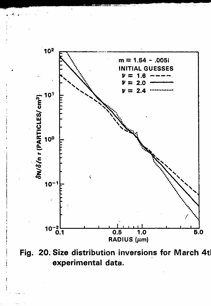
Other inverted size distributions with various initial guesses are

shown in Figs. 20 and 21. Twelve inversions were averaged and smoothed

to obtain a representative Inverted size distribution (Fig. 22). The

results are most closely modeled by a Junge size distribution with

m a 1.50 - .0351, v • 1.8, and mass loading of about 60 uglms . The curve

Is purposeiy truncated so that only the region of sensitivity is shown.

A maximum aerosol number concentration (or- turnover point) of the size

distribution is not observed since the sensitivity of the kernel drops

off sharply below 0.2 um while typical turnover points occur near 0.01 um

for the ground level Tucson aerosol.

(11)

VI. Conclusions and Further Study

The technique developed in this paper has yielded estimates of

atmospheric aerosol characteristics--vis., size distributions and real

and imaginary indices of refraction--from measurements of matrix

scattering elements at various angles. The results are reasonable in

comparison with other wor09-22

in this field, and the size distributions

match quite well near 0.1 um with , nuclepore filter measurements 16 that

were made at the same location but are sensitive to particles from

0.1 um on down.' To achieve a characterization of the ground level

Tucson aerosol, measurements should be made routinely over an extended

period.

Improvement in the stability of the inversion technique might be

achieved by smoothing the kernels to remove the higher frequency informa-

tion. Further sophistication could be achieved by expanding the inversion

routine to include fitting the inversion results to a smooth analytic

function and using this as a new first guess.

A detailed study ' of the information content would be of special

Interest. Initial work in this area has shown that the scattering data

used in this study are in the region of optimum information content.

This could lead to an instrument with a minimum number of fixed detectors

set at carefully chosen angles which would eliminate the need to move

the detector and speed the measurement time.

The author would like to thank Dr. Benjamin M. Herman and Dr. Walter H.

Evans for their assistance on this project. This research was funded by

the Office of Naval Research under Grant 000014-75-C-0208, and computer

time was furnished by the National Center for Atmospheric Research which

Is sponsored by the National Science Foundation, under project #35021004.

(12)

References

1. M. Z. Hansen, Apps. Opt. submitted for publication.

2. R. G. Pinnick, D. E. Carroll, and D. J. Hofman, Appl. Opt. 15,

384 (1976).

3. P. Chylek, G. W. Grams, and R. G. Pinnick, Science 193, 480 (1976).

4. C. Acquista, Appl. Opt. 17, 3851 (1978).

5. D. L. Phillips, J. Assoc Comput. Mach. 9, 84 (1962).

6. S. Twomey, J. Assoc. Comput. Mach. 10, 97 (1963).

7. S. Twomey, Mon. Wea. Rev.. 94, 363 (1966).

8. G. Yamamoto and M. Tanaka, Appl. Opt., 8, 447 (1969).

9. M. D. King,'D. M. Byrne, B. M. Herman, and J. A. Reagan, J. Atmos.

Sci. 35, 2153 (1978).

10. E. R. Westwater and A. Cohen, Appl. Opt. 12, 1340 (1973).

11. M. J. Post, J. Opt. soc.-Am. 66, 483.(1976).

12, B. M. Herman, S. R. Browning, and J. A: Reagan, J. Atmos. Sci.

28, 763 (1971) .

13. D. M. Byrne, Ph.D. Dissertation, U. Arizona (1978).

14. S. Twomey, J. Comp. Phys. 18,188 (1975).

15. J. V. Dave, "Subroutines . for Computing the Parameters of Electro-

magnetic Radiation Scattered by a Sphere," IBM Report 320-3237

(IBM Scientific'Center, Palo.Alto, Calif., 1968).

16. M. D. King, J. Atmos. SO. 36, 1072 (1979).

17. S. Twomey, J. Atmos..Sci. 33, 1 073 (1976).,

18.- M. T. Chahine, J. Opt. Soc &ii. 58, 1634 (1968).

19. J. D. Lindberg and L. S. Laude, Appl. Opt. 13, 1923 (1974).

(13)

20. J. D. Spinhirne, J. A. Reagan, and B. M. Herman, J. Appl. Meteorol.

19, 426 (1980).

21. G. W. Grams, 1. H. Blifford, Jr., D. A. Gillette, and P. B. Russell,

J. Appl. Meteorol. 13, 459 0974).

22. J. A. Reagan, D. M. Byrne, M. D. King, J. D. Spinhirne, and B. M.

Herman, J. Geophys. Res. 85, 1591 (1980).

(14)

Figure Captions

Fig. 1. Junge size distribution curves.

Fig. 2. Two-slope size distribution curves. .

Fig. 3. Scattering element M2 integrated over Junge size distributions.

Fig. 4. Scattering element S21 integrated over a Junge size distribution

for two particle size ranges.

Fig. 5. Scattering element M2 integrated over a Junge size distribution

for two particle size ranges. j

Fig. 6. Weighted scattering element M 2 for single particles.i

Fig. 7. Weighted scattering element M l for single particles. P

Fig. 8. Scattering element M 1 for single particles.

Fig. 9• Scattering element M2 for single particles. 1

Fig. 10. Power spectrum of M2.

Fig. 11. Power spectrum of D21'

Fig. 12. Convergence of iterative inversion for theoretical data with j

no error.

Fig. 13. Theoretical size distribution inversions for various mass

loading initial guesses.

Fig. 14. Theoretical size distribution inversions for various Junge

slope initial guesses.

Fig. 15. Convergence of iterative inversion for theoretical data with

11 percent error.

Fig. 10. M2 scattering matrix element.

Fig. 17. S 21 scattering matrix element.

Fig. 18. Size distribution inversions for March 9th experimental data.

Fig. 19. Convergence of iterative inversion for experimental data with

various mass loading initial guesses.

Fig. 20. Size distribution inversions for March 4th experimental data.

Fig. 21. Size distribution inversions for March 10th experimental data.

Fig. 22. Average of inverted size distributions.

am

a v

10,M

E

WJV

a 100a

sm

C

CIO

ZCIO

M -- 1.54 .0051MASS LOADING= 50 lig /m3

V = 2.0, V = 3.0

V= 4.0 ........................

PARTICLE DENSITY

tiA = 2g/Cm3

,

10-1

\ 10' 20.1 1.0 10.0

RADIUS ([Lm)

Fig. 1. Junge Size distribution curves.

Ub

104

E 102

LU

V 101

4CL

10°

CAD

^ 10-1

10-2

V1 V2 rA (Am)1) 2.0 1.5 .042) 2.0 1.0 .04'

3) 2.0 0.0 .04

4) 2.3 0.0 .01

5 2.3 -0.5 .01PARTICLE DENSITYp = 2g/cm3

3 ••

•

• ••'

1 •.

m = 1.54 - .005i -•.^000rB = 0.4 jim

MASS LOADING = 50 /ig/m3

. 103

10-3 1 - t i t 1 111 1 1. 1 I J 11111 1 1 1 1 1 1111

0.01 0.1 1.0 10.0\ RADIUS (µm)

Fig. 2. Two-slope size distribution curves.

ply' I3QUfXLITY,

E

N

.02<r<8.2µmPARTICLE DENSITY p = 2g/cm3

10-4

10-5

In1

10-1

10-2

10-3

m= 1.50 --.00iA = 0.5145 µm

MASS LOADING = 100 µg/m3

Y 2.0V3.0 .^- r^ r .^r

P = 4.0

♦

^• ♦``

*an woo

^•

0 20 40 60 80 100 120140 160 180SCATTERING ANGLE (DEGREES)

Fig. 3. Scattering element M 2 integratedover Junge size distributions.

a

101

10°

10`1

i,E 10-2

N

10-3

m= 1.54—.0051V = 3.0A= 0.5145 µmUPPER CURVE .02 < r < 8.2 µmLOWER CU RVE .02 < r < 2.0 jim

MASS LOADING = 100 µg/m3(FOR UPPER CURVE)

i`POSITIVEVALUES

}i{

i

4

NEGATIVEVALUES

10-4

10-5 10 20 40 60 80 100 120140 160 180

SCATTERING ANGLE (DEGREES)

Fig. 4. Scattering element S 21 integrated over aJunge size distribution for two particle sizeranges.

OF POOR QUALI"1'Y

i •^ 1

i

10

10°

10-1

r..E 10-2

N

m = 1.54 -- .005iY=3.0A= 0.5145 µmUPPER CURVE .02 < r < 8.2 jimLOWER CURVE .02 < r < 2.O jim

MASS LOADING = 100 jig/m3(FOR UPPER CURVE)

/,

10-3

10-4

i10-51 I I I I I I I I

0 20 40 60 80 100 120 140 160 180

SCATTERING ANGLE (DEGREES)

Fig. 5. Scattering element M 2 integratedover a Junge size distribution for twoparticle size ranges.

101

0 20 40 60 80 100SIZE PARAMETER,

Fig. 6. Weighted scattering element M2for single particles,

ri

10--7u

10-5

10_$

10-3

10_4

zo 40 60 s0 100SIZE PARAMETER, a

i

10°

• 10 -1

10-2

Fig. 7, Weighted scatterin elementment IVI,for single particles,

102

101

10°

10-1

j 10-2

10-3{i 10-4

-510 0

it

m 1.54-.003i8 - 34°

20 40 60 80 100

SIZE PARAMETER, ar

Fig. 8. Scattering element M1for single particles, ,

103

10`2

10-3

10-4

10'5

m = 1.54 -.003i8 = 176°

0 20 40 60 80

100SIZE PARAMETER, a

Fig. 9. Scattering element M 2 for singleparticles. .

1010

109

w ^R

m-- 1.54-.01i8 = 176°

f

0 50 100 150 200 250

FREQUENCY

Fig. 10. Power spectrum of M .2

<r''.I:,ii1t^I, PACs TS

POOR

m= 1.54 -.01i=34°109

1010

' 0i 50 100 150 200 250FREQUENCY

Fig. 11. Power spectrum of D21

^o0 ULM

i L

1

I •

t

i

LO

Ln L

M .o o

sm

1 4 ia ° >o 4)

Z ,>0

O .^.+

L.L. CO) Ln E"

c = c ecc

H ^-a

O v Z3i o w ( Ri

/ a' O/O

' so V +r

cqr-

o Lo

W UOUU3 SWUORIGI T- r 1)4 ( ^ i3nl, I't , rr y

. one

101Co

E

JV

OC 100aV

Z

10-1

10-2 ^--0.1

1m= 1.54-.005iV = 2.0

NO ERROR IN DATAMASS - LOADING = 38 µg/m3

INITIAL GUESSESm.1. = 15 µ.g/m3 ......

i m.1. = 100 11g/m3 _..._1 : ;CORRECT SOLUTION ._.

iH

oi lt j i l t` 1 1 ^, •.

^ ^,^ 11 ! 1 1 1^`

M i =^ 1 t Alts.

lose

• ^i 1 1 1 n

1 1 yll^^ ^^ ^ ^

r'

.,

0.5 1.0 5.0

RADIUS (µm)

Fig. 13. Theoretical size distribution inversionsfor various mass loading initial guesses.

1C'

10

Mme`LV

WVI--Q 10'ac

CIO

zC-0

10-1

V.5 1.0 5.0RADIUS (µm)

Fig. 14. Theoretical size distribution inversions forvarious J unge slope initial guesses.

O"'GI1'A L, P:1r, r: ISOF Pooh ^I)r^ r r t ^,

}

at

i

}

r

i

i

ii

i

i

I

10-20..

F 31

44

Ln LN oi

1 44i i L

W N CE- Io

CDOC .J I i 1

Ln

t O' — O M tVcc

tU

!1a

to IIa^!^ lip iia a a l i

^'u.

,^ ;cv •

OW ..^ i•^ no

Ln L

w

00,^000

Cwoo son

O'm goes

M N O pe- P

til 1101Ja3 swaii

•

101

10-4

•10-5

uu 180SCATTERING ANGLE (DEGREES)

Figs 16. M 2 scattering matrix element.

10 ^

10°

10_4

10-5

MARCH 9TH DATA WITH THEORETICAL

BEST FIT

V.=2.0m = 1.50--.0051

MASS LOADING = 38 µg1 m3

REPRESENT NEGATIVE VALUES

•

•

® • O O 1

ao • ^1it O

11

0 90 180

SCATTERING ANGLE (DEGREES)

Fig. 17. S 21 scattering matrix element.I

i

10-2

10-,{ E

WJ

V

a 100CL

CIO

ZCo

. 0 % " %:

M = 1.50 - 005iINITIAL GUESSES

y = 1.6 - - -y = 2.0 --y = 2.4 ..,,,.,,.

•. i

1 '

t .^

5.0102 L

0.1 0.5 1.0

i

1^^"

3• 1

10

S

RAD 1 U S (µm)

Fig.18. Size distribution inversions for March 9thexperimental data.

Il.

.^

Coboll

am

c tv^w ^

tJ ^ +r

0 , Xt0O

0 0 SPERMS

r

Ch

U.

InN

N

toZO

In

Wl000

U.

OO ^

'r DO

Z

In

^OO

li1 i

•i

W iW

1.

Zo 1W Z .}.1 .

O C7 1

W Q Z 1 •̂

1 •

Q •Z W O 1V~ J 1 1'1 i i• i

N> N 1 i• i'0 co

O W E E .J `^ ^•

i'

loo' 1 '

— 1 .

1^ O V ^ Z co P,O N p '.r.

11 11 ? O iii it tt it ;

E E E E 1 '

wopwoo woo amw

a^

OM ^ M

{^^o) aoaa3 swa

ORIGINAL PAGE ISOE POOR QUALITY

ti

to

Z.40

10-1

I

m = 1.54 -.005iINITIAL GUESSES

V = 2.0 -----w-.,^ y _ 2.4 ..............

M 10^E

WJv

H100a

il

RADIUS (µm)

I Fig. 20. Size distribution inversions for March 4thexperimental data.

OF

i

•^., m = 1.50 - .003i

INITIAL GUESSESs V= 1.6 ---

V= 2.0 -----V ..» 2.4 .........

%I

102

101two%ME

'W

V

CC 100C1.No

CIO

Z

CIO

10-1

` •a

•

1

I i

ir

%\

10-21 1 t --L--.Li fi ll0.1 0.5 1.0 5.0

RADIUS(Am)

Fig. 21. Size distribution inversions for March 10thexperimental data.

Ci,.I 1 ' .^L P k^;E IS

OF POOR QUALITY

m = 1.50 -.005i

101Cl)

EV

W.JV

0~C 100Qaownc^o

Z

`O 10-1

10-2 L0.1

0.5 1.0

5.0

RADIUS (µmj

Fig. 22. Average of inverted size distributions.