Embed Size (px)
Citation preview

MULTI-SCALE CHARACTERIZATION AND MODELING OF SHEAR-TENSION INTERACTION IN
WOVEN FABRICS FOR COMPOSITE FORMING AND STRUCTURAL APPLICATIONS
by
Mojtaba Komeili
M.A.Sc., The University of British Columbia, 2010
B.Sc., Iran University of Science and Technology, 2008
A THESIS SUBMITTED IN PARTIAL FULFILLMENT OF
THE REQUIREMENTS FOR THE DEGREE OF
Doctor of Philosophy
in
THE COLLEGE OF GRADUATE STUDIES
(Mechanical Engineering)
THE UNIVERSITY OF BRITISH COLUMBIA
(Okanagan)
April 2014
© Mojtaba Komeili, 2014

ii
Abstract
Woven fiber-reinforced polymer composites have become superior materials of choice in
advanced industries such as aerospace, energy and automotive. The low in-plane shear stiffness
of woven fabrics provides them with high formability, and hence the characterization of this
stiffness is of high impotence. Although it was assumed in the past that a fabric’s shear modulus
is merely a function of its shear angle, recent evidences show that this material property is also
dependent on other factors such as tension along yarns. However, there are currently difficulties
to fully characterize the level of this shear-tension interaction.
In this thesis, two different approaches are proposed to tackle the above characterization
problem: (1) experimental measurements using a newly developed test fixture; (2) virtual
experiments, which can greatly decrease the characterization cost. However, the input data for
the virtual experiments including material properties for yarns must be provided. Accordingly, a
new inverse identification approach using results of two conventional tests, (1) uni-axial tension
and (2) shear frame tests with initial pre-tension, were used along with a multi-objective genetic
algorithm optimization to arrive at material properties of yarns. Then, virtual experiments at
meso-level are conducted to extract the response surface of a selected fabric (TWINTEX
polypropylene/glass plain weave) under general in-plane combined shear-tension loadings. The
outcome was used in studying twisting moment response of inflatable structures reinforced with
woven fabrics as well as stamping process of the TWINTEX using three different punch and
mold geometries. Eventually, a comparison between earlier models (without interaction between
shear and tension modes) and the new model with shear-tension interaction is presented and
practical recommendations are made for enhanced fabric simulations.

iii
Table of Contents
Abstract .......................................................................................................................................... ii
Table of Contents ......................................................................................................................... iii
List of Tables ............................................................................................................................... vii
List of Figures ............................................................................................................................. viii
List of Symbols ......................................................................................................................... xviii
List of Abbreviations ................................................................................................................ xxii
Acknowledgements .................................................................................................................. xxiii
Dedication ................................................................................................................................. xxiv
Chapter 1: Introduction ...............................................................................................................1
1.1 Fiber reinforced composites ............................................................................................ 2
1.2 Textile composites .......................................................................................................... 3
1.3 Manufacturing of woven fabric composites ................................................................... 6
1.4 Multi-scale nature of woven fabrics ............................................................................... 9
1.5 Homogenization ............................................................................................................ 11
1.6 Motivation and objectives ............................................................................................. 12
1.7 Thesis outline ................................................................................................................ 14
Chapter 2: Background ..............................................................................................................17
2.1 Mechanical behavior of woven fabrics ......................................................................... 17
2.2 Draping and forming simulation of woven fabrics ....................................................... 19
2.2.1 Geometrical models .................................................................................................. 20
2.2.2 Discrete models ......................................................................................................... 21
2.2.3 Semi-discrete models ................................................................................................ 25

iv
2.2.4 Continuous models.................................................................................................... 28
2.3 Summary ....................................................................................................................... 29
Chapter 3: Fundamentals of macro-level fabric simulation using continuous models ........31
3.1 Thin-shell structures...................................................................................................... 31
3.2 Modeling of shells......................................................................................................... 32
3.3 Shell models used in Abaqus ........................................................................................ 34
3.4 In-plane elastic material model for dry fabrics ............................................................. 35
3.5 Built-in fabric material model of Abaqus ..................................................................... 38
3.5.1 FORTRAN subroutine for fabric material model of Abaqus ................................... 39
3.6 Summary ....................................................................................................................... 39
Chapter 4: Conducted experimental characterization techniques .........................................40
4.1 Importance of experimental data and formulations ...................................................... 40
4.2 Fabric material .............................................................................................................. 41
4.3 Uni-axial tension on fabrics .......................................................................................... 43
4.3.1 Conducting the test ................................................................................................... 44
4.3.2 Nominal uni-axial response ...................................................................................... 51
4.4 Shear test on fabrics ...................................................................................................... 53
4.4.1 Bias extension test..................................................................................................... 53
4.4.2 Shear/picture frame test ............................................................................................ 55
4.4.3 Digital Image Correlation (DIC) ............................................................................... 59
4.4.4 Preparations for shear frame test............................................................................... 64
4.4.4.1 Sample sizes ...................................................................................................... 64
4.4.4.2 Preparation of specimens and test fixtures........................................................ 64

v
4.4.5 Conducting the shear frame experiment ................................................................... 66
4.4.5.1 Shear frame test results without pretension ...................................................... 67
4.4.5.2 Pre-tensioning the fabrics ................................................................................. 69
4.4.5.3 Results of shear frame test after pre-tensioning ................................................ 71
4.4.5.4 Challenges in shear frame test .......................................................................... 72
4.4.6 Combined shear-tension loading test fixture ............................................................ 74
4.5 Summary ....................................................................................................................... 79
Chapter 5: Meso-level model development...............................................................................80
5.1 Introduction ................................................................................................................... 80
5.2 Finite element simulation of fabric at meso-level ......................................................... 80
5.2.1 Geometrical details ................................................................................................... 82
5.2.1.1 Unit cell ............................................................................................................. 82
5.2.1.2 The yarn and yarn path geometry ..................................................................... 83
5.2.2 Boundary conditions ................................................................................................. 84
5.2.3 Material constitutive model for yarns ....................................................................... 90
5.2.4 Hypo-elastic modeling and yarn orientation considerations ..................................... 93
5.2.4.1 Transforming Stress and Strain matrices (TSS)................................................ 97
5.2.4.2 Transforming Stiffness Matrix (TSM) .............................................................. 98
5.2.5 Comparing TSS and TSM in practice ....................................................................... 98
5.3 Inverse identification .................................................................................................. 101
5.4 Multi-objective optimization ...................................................................................... 105
5.5 Implementation of multi-objective optimization for current case study ..................... 107
5.5.1 Extracting global force response from nodal reaction forces ................................. 111

vi
5.6 Results of inverse identification.................................................................................. 114
5.7 Validation .................................................................................................................... 117
5.8 Summary ..................................................................................................................... 118
Chapter 6: Macro-level model development and its applications ........................................119
6.1 Effect of combined loading ......................................................................................... 119
6.2 Extraction of response surface functions for the combined loading ........................... 124
6.3 Application 1: the behavior of inflatable structures .................................................... 127
6.4 Application 2: simulation of fabric forming ............................................................... 129
6.4.1 Hemisphere forming ............................................................................................... 132
6.4.2 Double dome benchmark forming .......................................................................... 141
6.4.3 Tetrahedral punch forming ..................................................................................... 151
6.4.4 Concluding remarks on forming simulations with tension-shear coupling ............ 159
6.5 Summary ..................................................................................................................... 161
Chapter 7: Summary, Conclusions, and Future work ..........................................................163
7.1 Summary ..................................................................................................................... 163
7.2 Conclusions ................................................................................................................. 166
7.3 Future work ................................................................................................................. 168
Bibliography ...............................................................................................................................170
Appendices ..................................................................................................................................181
Appendix A: FORTRAN subroutines for meso-level model .................................................181
Appendix B: Transformation matrix of fibers ........................................................................194
Appendix C: FORTRAN subroutine for macro-level model .................................................198

vii
List of Tables
Table 4-1. Specifications of the fabric material used in this research, reported by
woven fabrics benchmark forum (http://www.wovencomposites.org) ......................42
Table 4-2. Average strains in the region of interest after pre-tensioning ...................................71
Table 5-1. Details of applying boundary conditions using the general formula (Eq.
5.5) for each loading mode .........................................................................................88
Table 5-2: Obtained axial stresses (σz) using different combinations of
integrator/material models and their error percentages compared to the
analytical solution of the problem shown in Fig. 5-8 ...............................................100
Table 5-3. Result of inverse identification .................................................................................115
viii
List of Figures
Figure 1-1. Different types of fibers in composites in general .......................................................3
Figure 1-2. Selected types of textile reinforcements that are common in composite
materials (Sherburn, 2007) ...........................................................................................4
Figure 1-3. Three different fabric types and the geometrically repetitive element .........................5
Figure 1-4. Four common techniques of composite manufacturing on woven fabrics;
(a) resin transfer molding (RTM); (b) forming of pre-impregnated fabrics;
(c) thermo-stamping; (d) hydro-forming, the flexible die is formed under
the pressure from punch. Note that (a) and (b) are mostly used for thermo-
set matrices whereas (c) and (d) are for thermo-plastics. .............................................7
Figure 1-5. The multi-scale nature of woven fabrics and the schematic of modeling
assumptions for each scale .........................................................................................11
Figure 1-6. Homogenization of different material scales for woven fabrics .................................12
Figure 1-7. Outline of the topics discussed in each chapter ..........................................................16
Figure 2-1. Kawabata model for meso-level modeling of plain woven fabrics.............................18
Figure 2-2. Discrete models for studying fabric deformation; (a) yarns are modeled by
1D stiffness (translational and rotational spring) elements (Ballhause et al.,
2006); (b) yarns are modeled by shell elements (Gatouillat et al., 2010);
(c) yarns are modeled by solid elements (Tavana et al., 2012) ..................................23
Figure 2-3. The discrete model of macro-level deformation taking into account micro-
level details; (a) fabric geometry before deformation (Durville, 2005); (b)
fabric geometry after deformation (Durville, 2007) ...................................................24
Figure 2-4. The bilinear element in a semi-discrete model (Boisse, 2006) ...................................25

ix
Figure 2-5. Semi-discrete model; (a) the selected unit cell of the fabrics and applied
loads, note that ii subscript is used instead of i for 1 and 2 (Hamila et al.,
2009); (b) loads on the unit cell in decoupled form shown in 3D (Allaoui
et al., 2011) .................................................................................................................27
Figure 3-1. The basic loading modes on a shell: (a) in-plane modes; (b) bending modes ............34
Figure 3-2. Coordinate systems used for simulating the deformation of woven fabrics;
(a) orthogonal coordinate systems before deformation; (b) non-orthogonal
covariant (along yarns) and contravariant coordinate system after
deformation ................................................................................................................37
Figure 4-1. A photo from the fabric samples used in the experiment along with the
geometrical features of its unit cell (spacing, width and thickness) ...........................42
Figure 4-2. Fixture used for uni-axial tension and the schematic of resulting
deformation ................................................................................................................43
Figure 4-3. Instron 5969 universal tension/compression machine ................................................44
Figure 4-4. Response of the fabric to axial tension under five repeats, (a) loading along
warp direction; (b) loading along weft direction ........................................................46
Figure 4-5. Response of the extracted yarns to axial tension, (a) yarns extracted along
warp direction; (b) yarns extracted along weft direction ...........................................48
Figure 4-6. Raveling of the fabric specimen after mounting into the test fixture with
small pretension ..........................................................................................................49
Figure 4-7. Response of the ravelled fabric to axial tension under five repeats, (a)
loading along warp direction; (b) loading along weft direction .................................50

x
Figure 4-8. The averaged axial response of the fabric, ravelled fabric and yarns, (a)
along warp direction; (b) along weft direction ...........................................................51
Figure 4-9. The nominal axial response of the fabric to axial strain along warp and
weft used in the subsequent models ...........................................................................52
Figure 4-10. (a) Bias extension (BE) test fixture (Peng & Cao, 2005); (b) the
schematic of deformation regions; the ideal shear angle in each regions:
C=0, B=γ/2 and A=γ ...................................................................................................54
Figure 4-11. (a) Biaxial bias extension (BBE) test fixture developed by Harrison et al.
(2012); (b) the specimen and ideally distinct deformation zones ..............................55
Figure 4-12. (a) A conventional shear frame test fixture; (b) schematic of the test and
resultant deformation on fabric ..................................................................................56
Figure 4-13. (a) Shear frame test fixture used in this study; (b) schematic of the fixture
and clamping mechanism, bolts on the top are pressing fabric between
clamping parts by pushing the orange piece down. Fabric is pressed
between the bottom of orange part and the internal floor of the blue part.
After placing the fabric, bolts on the sides can be tightened to apply pre-
tension. .......................................................................................................................58
Figure 4-14. The placement of cameras in a relative angle to the specimen for
stereovision .................................................................................................................61
Figure 4-15. Three different sizes of calibration plates for the DIC system which can
be used for experiments in different characteristic lengths ........................................62
Figure 4-16. Image processing for calculation of deformation in DIC, images taken
from left and right cameras are shown together; (a) the facets made on the

xi
surface of specimen in Instra4D® software; (b) the reconstructed plane on
the surface ...................................................................................................................63
Figure 4-17. The geometry of specimens used in the shear frame test ..........................................64
Figure 4-18. The preparation of specimens for shear frame tests; (a) alignment of the
fixture and placing the fabric holder; (b) cutting fabric samples and
drawing the alignment lines; (c) clamping fabric inside the fixture and
placing the foam on top and installing the fixture inside the tension
machine, foam is removed right before the test. ........................................................66
Figure 4-19. The spacers are used in the shear frame fixture to run experiments with
pre-tension. They are removed after placing the fixture in the Instron
machine. Then bolts on the sides are tightened to induce tension. ............................67
Figure 4-20. The outcome of shear frame test with no pre-tension ...............................................68
Figure 4-21. Measurement of average strain over the surface of the specimen after pre-
tensioning; (a) surface constructed through DIC before pre-tensioning; (b)
after pre-tensioning; (c) the state of calculated strain over the region of
interest ........................................................................................................................70
Figure 4-22. The outcome of shear frame test with pre-tension (as reported in Table 4-
2) .................................................................................................................................72
Figure 4-23. Wrinkles developed in the fabric during the shear frame test (surface
generated by DIC) ......................................................................................................73
Figure 4-24. First test fixture developed for studying the effect of combined loading by
UBC, NUWC and CCNY, (a) the fixture inside a tensile machine; (b) the
status of fabric inside the fixture ................................................................................76
xii
Figure 4-25. Deformation of a cross shaped fabric under sliding shear and trellising
shear; (a) sliding shear: the cross over points are moving along the yarns
and yarns are sliding on each other; cross over point after deformation (red
region) is different from cross over points before deformation; (b)
trellising shear: cross over points are not moving relative to yarns and
yarns are pivoting around cross over points ...............................................................77
Figure 4-26. Three initially suggested designs for the new combined shear-tension
fixture .........................................................................................................................78
Figure 4-27. The newly developed test fixture for studying shear-tension coupling
effect; (a) final mechanical design; (b) final manufactured fixture (©
CCNY, UBC, NUWC) ...............................................................................................79
Figure 5-1. Selected unit cell for a balanced plain weave .............................................................83
Figure 5-2. Features of periodically repeating unit cell .................................................................85
Figure 5-3. Decomposition of deformation into macro-level and periodic deformations .............86
Figure 5-4. The corner points to apply the boundary conditions (red points); two
periodically paired points along the border line (blue points) ....................................88
Figure 5-5. Paired nodes in the meso-level model using a MATLAB code ..................................90
Figure 5-6. Tomography image showing fibers in a sample of woven fabric textile
composite laminate (courtesy of Dr. Shah Mohammadi, UBC Okanagan) ...............91
Figure 5-7. The deviation of initial material orientation/frame from the working frame
of finite element that should be considered during stress updates .............................93
Figure 5-8. The simple geometry used for comparing different stress update methods
and its loading condition (dimensions of cube are 20×20×20 mm) ...........................99

xiii
Figure 5-9: The normalized run-time for each simulation. Note that the simulation
could not converge for shear in the explicit integrator .............................................101
Figure 5-10. The discrete values of real response from experiment ( ) are compared
to the response predicted from model ( ) to obtain the residual/error ( ). ...........104
Figure 5-11. The Pareto front (a) with full mapping from space of variables to
objectives; P1 is dominated by several points including P2 and P3; (b)
Pareto front estimated with discrete values and limited number of data
points ........................................................................................................................107
Figure 5-12. The Isight flow-model used for running optimization process for inverse
identification of yarns material properties (details of each step is discussed
above) .......................................................................................................................111
Figure 5-13. Reaction forces on the nodal point for finding tension and shear forces on
the fabric ...................................................................................................................113
Figure 5-14. The force response of model characterized via inverse identification and
compared to the experimental results; (a) uni-axial tension; (b) shear frame
with pre-tension .......................................................................................................115
Figure 5-15. Some of data points generated during the optimization process in inverse
identification; the red points are those on the Pareto front where the blue
point shows the optimum point selected using the above mentioned
weighting and scale functions ..................................................................................116
Figure 5-16. Validating the response of the model using the shear frame experimental
results ........................................................................................................................118

xiv
Figure 6-1. The axial stress response of the unit cell to different combinations of axial
strain and shear levels ...............................................................................................121
Figure 6-2. The shear stress response of the unit cell to different combinations of axial
strain and shear levels ...............................................................................................122
Figure 6-3. Comparing the response of the fabric to different sequences of loading for
the same level of deformation; (a) the axial response along yarns (b) shear
response ....................................................................................................................124
Figure 6-4. The axial stress response of the unit cell and the fitted function; different
surfaces are representing different levels of γ ..........................................................126
Figure 6-5. The shear stress response of the unit cell and the fitted function; different
surfaces are representing different levels of ε1 .........................................................126
Figure 6-6. The geometry of an inflatable beam/shaft under torsion ..........................................128
Figure 6-7. (a) The difference in the torsional response of the inflatable beam to
different internal pressures and twist angles; (b) the percentage difference
between predicted torsional moment between two models with and
without shear-tension coupling ................................................................................129
Figure 6-8. Shear stiffness of the fabric as a function of strain along yarns and shear
angle, extracted from stress response formulas ........................................................130
Figure 6-9. (a) The geometry of the forming simulation; blue edges in the shell are the
symmetric boundary conditions; (b) the dimensions of tools ..................................133
Figure 6-10. Comparison of predicted shear stress in forming with a hemisphere punch
using the uncoupled and coupled models (units in Pa); a blank-holder
force of 200N is used in the simulation ....................................................................135

xv
Figure 6-11. Comparison of predicted relative/shear angle in forming with a
hemisphere punch using the uncoupled and coupled models (units in
Radians); a blank-holder force of 200N is used in the simulation ...........................136
Figure 6-12. Comparison of the predicted shear stress in forming with a hemisphere
punch using the uncoupled and coupled models (units in Pa); a blank-
holder force of 25N and pre-tensioning force of 400 N/m are used in the
simulation .................................................................................................................138
Figure 6-13. Comparison of the predicted relative/shear angle in forming with a
hemisphere punch using the uncoupled and coupled models (units in
radians); a blank-holder force of 25 and pre-tensioning force of 400 N/m
are used in the simulation .........................................................................................139
Figure 6-14. The shear angle distribution along a selected path line in hemisphere
forming: (a) the location of line on the formed fabrics; (b) the values of
shear angle along the line as a function of distance from the center of
hemisphere ................................................................................................................140
Figure 6-15. Validating the forming model; (a) the shear angle (in radians) using the
current coupled model; (b) the shear angle (in degrees) using uncoupled
model (Jauffrès et al., 2011) .....................................................................................141
Figure 6-16. The geometry of the double dome model; only a quarter of the fabric is
simulated and symmetric boundary conditions are applied at the blue
highlighted edges of the fabric. ................................................................................142

xvi
Figure 6-17. Comparison of the predicted shear stress in forming with a double dome
punch and mold using the uncoupled and coupled models (units in MPa); a
blank-holder force of 100N is used in the simulation ..............................................143
Figure 6-18. Comparison of the predicted shear/relative angle in forming with a double
dome punch and mold using the uncoupled and coupled models (units in
radians); a blank-holder force of 100N is used in the simulation ............................144
Figure 6-19. The axial strain along weft (ε2) in the double-dome forming case .........................146
Figure 6-20. Comparison of the predicted shear stress in forming with a double dome
punch and mold using the uncoupled and coupled models (units in MPa); a
blank-holder force of 10N and pre-tensioning force of 400 N/m are used in
the simulation ...........................................................................................................147
Figure 6-21. Comparison of the predicted shear/relative angle in forming with a double
dome punch and mold using the uncoupled and coupled models (units in
radians); a blank-holder force of 10N and pre-tensioning force of 400 N/m
are used in the simulation .........................................................................................148
Figure 6-22. The shear angle distribution along a selected path line in double dome
forming: (a) the location of line on the formed fabrics; (b) the values of
shear angle along the line as a function of distance from the start point .................150
Figure 6-23. Validating the model; (a) the predicted shear angle (in radians) using the
newly developed model; (b) the predicted shear angle (in degrees) in the
simulation conducted by (Peng and Rehman, 2011) ................................................151
Figure 6-24. The geometry of tetrahedral punch and fabric ........................................................152
xvii
Figure 6-25. Comparison of the predicted shear stress in forming with a tetrahedral
punch using the uncoupled and coupled models (units in Pa); a blank-
holder force of 200N is used in the simulation ........................................................153
Figure 6-26. Comparison of the predicted shear/relative angle in forming with a
tetrahedral punch using the uncoupled and coupled models (units in
radians); blank-holder force of 200N is used in the simulation ...............................154
Figure 6-27. Comparison of the predicted shear stress in forming with a tetrahedral
punch using the uncoupled and coupled models (units in Pa); blank-holder
force of 200N and pre-tensioning force of 400 N/m are used in the
simulation .................................................................................................................155
Figure 6-28. Comparison of the predicted shear/relative angle in forming with a
tetrahedral punch using the uncoupled and coupled models (units in
radians); a blank-holder force of 200N and pre-tensioning force of 400
N/m are used in the simulation .................................................................................156
Figure 6-29. The shear angle distribution along a selected path line in tetrahedral
forming: (a) the location of line on the formed fabrics; (b) the values of
shear angle along the line as a function of distance from the start point .................158
Figure 6-30. The out of plane displacement of the fabric (representing wrinkles) in the
tetrahedral forming predicted from the uncoupled model in comparison to
the coupled model ....................................................................................................161

xviii
List of Symbols
Symbol Definition
Material constitutive tensor (Fourth order tensor)
[ ]
In-plane stiffness matrix in non-orthogonal coordinate system
, Objective derivative of stress tensor (Second order tensor)
Deformation gradient tensor (Second order tensor)
Spatial rate of deformation tensor (Second order tensor)
Polar rotation tensor (Second order tensor)
The right stretch tensor (Second order tensor)
The left stretch tensor (Second order tensor)
Spin rate tensor (Second order tensor)
[ ] In-plane stiffness matrix in orthogonal coordinate system
Strain rate tensor (Second order tensor)
Transformation tensor (Second order tensor)
The unit base vectors for working frame of the FE package
The unit base vectors along the fiber direction in a yarn
General strain tensor component in a non-orthogonal covariant coordinate
system
General stress tensor component in a non-orthogonal contravariant coordinate
system
Displacement boundary (boundaries with known displacement values)
Traction boundary (boundaries with known traction force values)

xix
Normalized shear force in the shear frame test
Shear force in the shear frame test or unit cell
,
Tension force along yarns in warp or weft direction at meso-level in the unit
cell
The shear stiffness of the yarns
Transverse shear stiffness in a shell element
Length of the region of interest in the shear frame test
Length of the arms in the shear test fixture
In-plane shear moment of the fabric element in each unit cell (semi-discrete
model)
Bending moment of the fabric shell model in each unit cell (semi-discrete
model)
Bending/twisting components of moment per unit length in a shell
Axial and shear components of in-plane force per unit length in a shell
Transformation tensor between orthogonal and non-orthogonal coordinates
Tension along yarns in each unit cell (semi-discrete model)
Virtual work from the acceleration
Virtual work done by the external forces
Virtual work done by the internal energy storage
Virtual work done by the internal energy storage due to fabric bending
Virtual work done by the internal energy storage due to in-plane shear
Virtual work done by the internal energy storage due to tension along yarns
( ) Suggested function in an inverse identification with a vector of constants,
[ ] Transformation matrix from the frame of fabric to the frame of FE software

xx
[ ] Transformation matrix from the frame of FE software to the frame of fabric
(inverse of [ ])
[ ] Transformation matrix between an orthogonal and non-orthogonal coordinate
system
Base unit vectors in an orthogonal coordinate system
The 3D vector of body forces
The 3D vector of traction forces
Base unit vectors in a non-orthogonal contravariant coordinate system
Base unit vectors in a non-orthogonal covariant coordinate system
In-plane shear strain of shell elements
In-plane axial strain of fabric along yarns
General strain tensor in an orthogonal coordinate system
The scale factor of parameter l in total objective function
Stretch value along warp or weft
The Poisson’s ratio of the yarns
In-plane axial stress components along yarns
General stress tensor in an orthogonal coordinate system
In-plane shear stress of fabric material
Curvature for a fabric shell element
The weight factor of parameter l in total objective function
Vector containing in-plane strains for a shell element
E22, E33 Transverse stiffness of yarns
h Yarn height/thickness in a fabric unit cell
H Height of the specimen in Bias-Extension test

xxi
S Yarn spacing in a fabric unit cell
w Yarn width in a fabric unit cell
W Width of the specimen in Bias-Extension test
The domain of the medium
Volumetric Jacobian
( ) Output as an unknown function of the input vector
Displacement in moving head of the tension machine
The 3D displacement vector
The position vector
The boundary of the meso-level unit cell
Warp rotation angle
Trellis shear angle between warp and weft
The angle between the arms in a shear frame test fixture
The vector of virtual displacement field
( ) ‖ ( ) ‖
Euclidian norm for the vector ( ) which is a function of (material
constants)
( ) ( ) Error associated with predicting function in an inverse identification

xxii
List of Abbreviations
Abbreviation Definition
BBE Biaxial Bias Extension
BE Bias Extension
CAD Computer Aided Design
CAE Computer Aided Engineering
CCNY City College of New York
CRN Composites Research Network
DIC Digital Image Correlation
FE(M/A) Finite Element (Method/Analysis)
KES Kawabata Evaluation System
LRTM Light Resin Transfer Molding
NSERC Natural Sciences and Engineering Research Council of Canada
NUWC Naval Undersea Warfare Center
PP Polypropylene
RTM Resin Transfer Molding
SF/PF Shear Frame / Picture Frame
TWINTEX®
Commercial name for comingled E-glass Polypropylene fibers
VARTM Vacuum Assisted Resin Transfer Molding

xxiii
Acknowledgements
First I would like to thank my supervisor Dr. Abbas S. Milani who supported me during the
challenging times of my PhD research. He was my supervisor for the last 5 year from the
beginning of my graduate studies at Master’s level and I appreciate all his efforts,
encouragement and friendship. The financial support for this research was provided by Natural
Sciences and Engineering Research Council of Canada (NSERC). I want to show my gratitude to
NSERC and also industrial and academic collaborators of this project specially, Mr. Paul
Cavallaro from Naval Undersea Warfare Center (NUWC) and Dr. Ali Sadegh and his team of
capstone students from City College of New York (CCNY). Many thanks also go to my
members of supervisory committee Dr. Spiro Yannacopoulos, Dr. Frank Ko, Dr. Kian
Mehravaran and Dr. Reza Vaziri for their support and feedback during my studies, research, and
preparation of the thesis.
I would also like to thank all my friends in the Composites Research Network (CRN) as well as
UBC Okanagan and my close friends in Canada, Iran and all over the world. Unfortunately,
mentioning all of their names is not feasible in a few pages but I sincerely admire them for being
my source of motivation throughout my life. Last but not least, I show my gratitude to my lovely
parents who have tirelessly supported me to get to this stage of my academic career, and also to
my brother and sisters and their families for their continuous encouragement. Above all, I would
like to thank God almighty for providing me with the blessing of health and knowledge.

xxiv
Dedication
To my parents because of all their unconditional love & sacrifice for our family

1
Chapter 1: Introduction
A composite material can be generally defined as a system of two or more materials which are
combined but are not necessarily chemically dissolved one into another. In an engineering
context, the purpose of this mixture is to achieve a higher level of performance in the ensuing
material system, a level that could not be achieved from the individual constituent materials of a
composite. In the last decades with the rapid advancements in material processing techniques,
composite materials have proven to be an opportunity for enhanced design and manufacturing in
modern industries. The potential for performance-based design and robustness of parts that use
composite materials is far beyond capabilities offered by traditional engineering materials (such
as metals, ceramics and polymers). For instance, since World War II aerospace industries have
been using composite materials (fiber glass and polyester) in their secondary structures without
much load-bearing demands to reduce the weight of aircrafts (Soutis, 2005; Strong, 2008);
however, recent advancements in manufacturing of stronger reinforcement materials as well as
matrix materials have led to a vast development of composites that are now dominant materials
of choice for fuselage in most new aircrafts such as Boeing 787, Airbus A320 and Eurofighter
Typhon (Soutis, 2005).
Automotive industry has also been involved in composites application with a goal of optimizing
the car body weight and reducing manufacturing costs as well as increasing the car crash safety.
Lamborghini Inc. started the first design of carbon fiber chassis for the Countach prototype in
1982 that led to the state of the art carbon fiber monocoque of Aventador for the next generation
of supercars (Nothdurtfer and Oto, 2012). Other automobile manufacturers such as Ford and
Chevrolet explored the possibilities of using capabilities of composites for mass production of
car parts (Strong, 2008). Transportation, construction, marine, sports and leisure, and medical

2
industries are among other venues that have brought the composite materials more and more into
our daily life. Indeed, clay and adobe used by ancient civilization, laminates of metals and
plywood could also be categorized as composite materials (Kaw, 1997). Even the biological
systems have developed some sort of composites during their evolution; for example, wood
which is a combination of cellulose fibers in a natural glue, called lignin (Mazumdar, 2001).
1.1 Fiber reinforced composites
Fiber reinforced composites are one of the most widely used type of composites. They are
generally made of fibrous materials embedded inside another bulk material to satisfy some
mechanical, thermal, physical, etc. design requirements. These fibers are referred to as the
reinforcement because in structural composites, 70% to 90% of the load is carried by fibers
(Mazumdar, 2001). On the other hand, the bulk material is commonly known as the matrix, but
the name polymer or plastic is often used instead of matrix in the case of thermosetting or
thermoplastic composites (this naming may apply even if the reinforcement is made of polymer
based materials). Basically, the matrix bonds the fibers together; distributes the load between
them; protects fibers against the environmental conditions, among numerous other benefits for a
composite system as discussed by Mazumdar (2001).
Architecture and arrangement of fibers inside the matrix can have different forms such as (1)
continuous fibers, (2) random fiber mats and (3) short fibers as illustrated in Figure 1-1.
Generally speaking, continuous long fiber composites have the highest load bearing capacity and
the short fibers have the lowest (Strong, 2008).
3
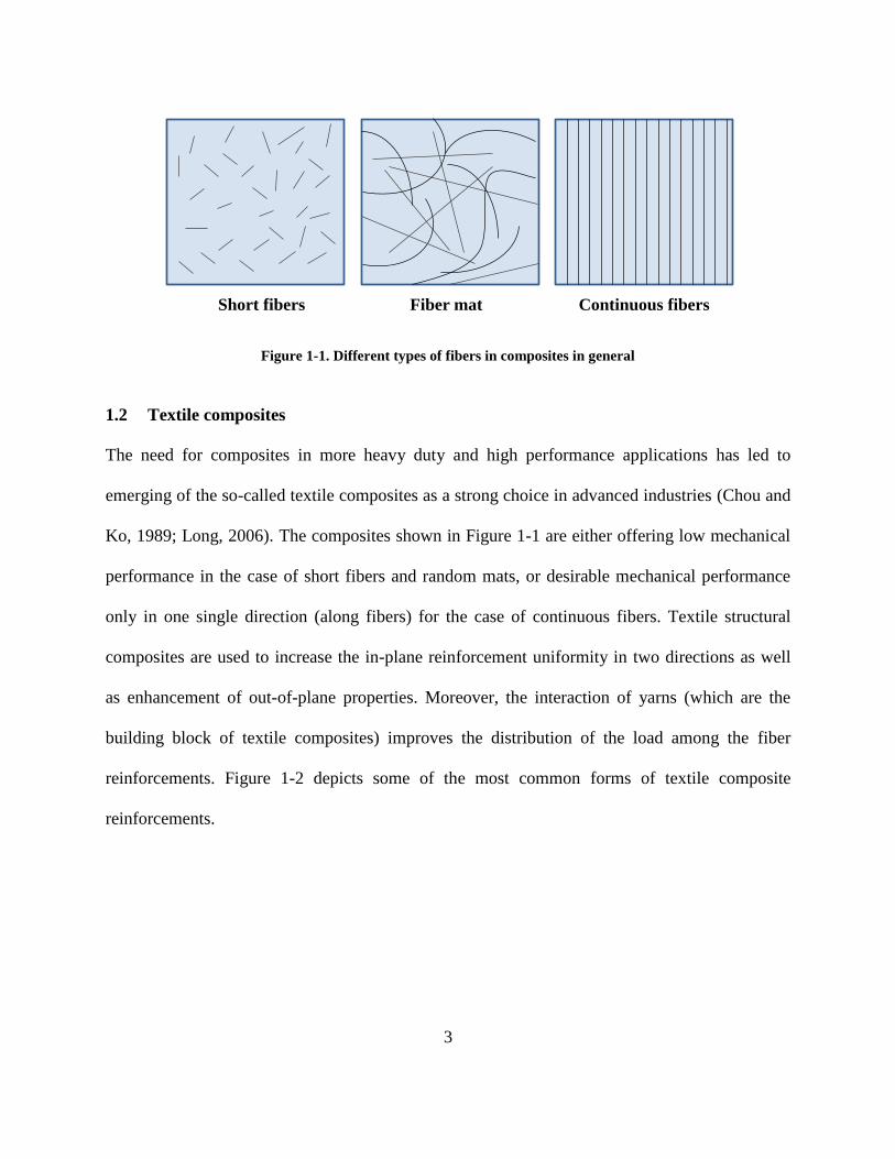
Figure 1-1. Different types of fibers in composites in general
1.2 Textile composites
The need for composites in more heavy duty and high performance applications has led to
emerging of the so-called textile composites as a strong choice in advanced industries (Chou and
Ko, 1989; Long, 2006). The composites shown in Figure 1-1 are either offering low mechanical
performance in the case of short fibers and random mats, or desirable mechanical performance
only in one single direction (along fibers) for the case of continuous fibers. Textile structural
composites are used to increase the in-plane reinforcement uniformity in two directions as well
as enhancement of out-of-plane properties. Moreover, the interaction of yarns (which are the
building block of textile composites) improves the distribution of the load among the fiber
reinforcements. Figure 1-2 depicts some of the most common forms of textile composite
reinforcements.
Short fibers Fiber mat Continuous fibers

4
Figure 1-2. Selected types of textile reinforcements that are common in composite materials (Sherburn, 2007)
Yarns are bundles of relatively long fibers. Each yarn is made of hundreds or thousands of fibers
which are continuous or discontinuous (in case of textile composites continuous fibers are
preferred due to better structural integrity). In addition to the base material of fibers, density of
fibers inside yarns is a crucial factor in properties of yarns. Therefore, there are engineering
parameters to characterize via measuring the linear density of yarns (Long, 2006). Some of the
most common parameters are:
Denier: mass in grams per 9000 meters of yarn length

5
Tex: mass in grams per kilometer of yarn length
Yarn count/number: Length of yarn per unit mass (imperial unit: pound/yard)
Yield: length per unit mass (imperial unit: yard/pound)
There are a vast number of different textile composites with different fiber architectures and
every year new textiles are introduced to the market. However, the main focus of this research is
on woven fabrics. Woven fabrics are made of interlacing of two or more yarn systems (Chou and
Ko, 1989). In the case of two-dimensional orthogonal yarns, interlacing yarns are referred to as
warp and weft. Essentially, manufacturing of woven fabrics is similar to manufacturing of
textiles in apparel industries, where a weaving loom is used to insert weft yarns in between warp
yarns (Long, 2006). Woven fabrics can be classified based on the pattern of interweaving in a
repetitive element. For illustration purpose three most common types of woven fabrics are shown
in Figure 1-3.
Figure 1-3. Three different fabric types and the geometrically repetitive element

6
1.3 Manufacturing of woven fabric composites
As mentioned above, composite materials are composed of at least two constituents known as
reinforcement and matrix. Woven fabrics have high drapability and can form into complex 3D
shapes in order to manufacture a variety of reinforced structures. In manufacturing of composite
materials, woven fabrics are formed into a desired three-dimensional surface shape and then
consolidated via different techniques such as Resin Transfer Molding (RTM) and its family such
as Vacuum Assisted RTM (VARTM), and Light RTM (LRTM) (Long, 2006), and open molding
for thermosetting composites (Cherouat and Billoe, 2001). Woven fabrics are also used
frequently in thermo-stamping (Sargent et al., 2010) or hydro-forming (Yu et al., 2003) of
thermoplastic composites. Figure 1-4 illustrates schematics of these manufacturing techniques.

7
Figure 1-4. Four common techniques of composite manufacturing on woven fabrics; (a) resin transfer
molding (RTM); (b) forming of pre-impregnated fabrics; (c) thermo-stamping; (d) hydro-forming, the
flexible die is formed under the pressure from punch. Note that (a) and (b) are mostly used for thermo-set
matrices whereas (c) and (d) are for thermo-plastics.
Basically, in the RTM techniques, the reinforcement material is formed into the desired shape of
the mold and then the liquid resin is transferred from a barrel to impregnate the fibers. Transfer

8
of resin to the fabric is done by pumping it into the mold cavity and sometimes implementing
vacuum (sink) on the opposite side at an optimum location found through simulation of resin
flow (Long, 2006). For pre-impregnated fabrics, the fabrics are already impregnated with the
liquid resin and it only needs to be formed and cured and find its solid form. These two
techniques are more common for thermoset matrices where the resin has low viscosity at low
temperatures. However, for the case of thermo-plastic matrices, because they are (commonly) in
solid form at room temperature, and after melting their viscosity is high due to large molecular
weights, they cannot be easily processed with similar techniques. Therefore, alternative methods
for assisting fiber wet-out in thermoplastics are explored as some of them are listed here (Strong,
2008):
1- Film stacking: stacking thin sheets of thermo-plastic consolidated polymer on top (or on
both sides) of the woven fabric preforms.
2- Powder coating: the gaps within the fabric are filled with the thermo-plastic powder.
Sometimes a skin material is added to protect powders from falling off.
3- Co-weaving: two sets of yarns made of reinforcement materials and matrix material are
woven together to form the fabrics.
4- Co-mingling: individual yarns in the fabric are made of continuous fibers from both
reinforcement material and matrix together.
All these solid impregnated fabrics can be used in thermo-stamping and hydroforming where
imposing temperature and pressure simultaneously or sequentially can melt the thermo-plastic
matrix and let the fiber wet-out occur. Afterwards, the cooling process is applied to bring the
matrix to a solid form and consolidate the final shape of the composite part. Particularly, the
latter solid impregnation method (co-mingling) has attracted considerable attention in the last

9
couple of decades and has led to invention of advanced, e.g., TWINTEX® fabrics which are
made of E-glass reinforcement fibers commingled with Polypropylene (PP) thermo-plastic
matrix fibers. These fabrics are commercially available in typical forms of plain and 2/2 twill
weaves. The plain TWINTEX is the main selected fabric for subsequent experimentations and
simulations in this research.
1.4 Multi-scale nature of woven fabrics
Heterogeneity of woven fabrics and composite materials in general is one of the most important
challenges in studying their behavior. Although, it is literally impossible to find a perfectly
homogeneous material, most of metals, ceramics and polymers can be assumed to behave close
to an ideally homogeneous material (before yield or damage). On the other hand, fiber reinforced
composite materials are inherently made of different constituents that are bonded together
without chemically dissolving. The ratio of these constituent materials as well as the architecture
of the reinforcement (random fiber mat, continuous fibers, or textiles) can greatly affect the
composite’s effective properties.
Essentially, woven fabrics can be considered as structured, hierarchical materials, having three
structural levels (Lomov et al., 2007). They include micro-level, meso-level, and macro-level
systems as follows:
1- Micro-level: this is the material level of individual fibers. In the case of textile structural
composites they are made of continuous filaments that are often composed of different
types of glass (E-glass, S-glass etc.), carbon/graphite or aramid materials. The length-to-
width ratio of fibers is very large and at the dry form (i.e., with no matrix or resin) this
makes them capable of only carrying high tensile loads (they easily buckle under

10
compression). The characteristic length in this scale depends on the type of fabric and
typically it is in the order of µm.
2- Meso-level: the bundle of fibers constitutes a yarn which is the main element of a fabric
in the meso-level. In a dry from (before resin injection) the only interaction between the
fibers are the forces due to contact and the friction. Essentially, these forces are not
enough to generate substantial stiffness in the shear and transverse loadings, but fibers
show a significant resistance to tension in the axial direction where loads are carried
along the fibers’ axis. In summary, the mechanical (and other) properties of yarns are
dependent on the interaction of fibers at the micro-level. The characteristic length of
elements (yarns) in this scale is normally in the order of mm.
3- Macro-level: this is the level of the final part made of textile composites. The
interweaving of yarns in meso-scale and their interaction is a crucial factor that dictates
the mechanical properties on the final part. The length scale for a macro-level study is
usually in the order of cm or m.
Figure 1-4 illustrates these three geometrical scales. As mentioned above, studying the
mechanical, thermal or physical behavior of woven fabrics at macro-scale (which is usually level
of interest for a product design) is affected by the meso-level elements (yarns) which are in turn
affected by the interaction between the fibers at the micro-level. Considering these elements,
with their interactions at different scales, leads to a complex analysis with a massive amount of
data that cannot be processed for a full-scale product design via capabilities of current
computers. Therefore, homogenization techniques have been suggested to ease this challenge.

11
Figure 1-5. The multi-scale nature of woven fabrics and the schematic of modeling assumptions for each scale
1.5 Homogenization
Due to the aforementioned complexity in studying the multi-scale materials and/or materials with
heterogeneity, homogenization techniques are proven as a powerful tool to analyze the behavior
of these materials at lower computational costs (Bakhvalov and Panasenko, 1989).
Homogenization in composite materials and particularly woven fabric composites (Sejnoha &
Zeman, 2008; Tabiei & Yi, 2002; Takano et al., 1999; Whitcomb et al., 1995) as well as dry
fabrics (Peng & Cao, 2002; Peng & Cao, 2000) has been implemented in finite element
numerical simulations in the past two decades.
The basic idea behind homogenization is to assume that the material in each higher level (e.g.,
meso and macro) is homogeneous. However, the material constitutive behavior is postulated in a
Micro-level
fibers
~10-6 m
Macro-level
part
~100 m
Meso-level
yarns
~10-3 m
Act
ua
lS
imu
lati
on
12
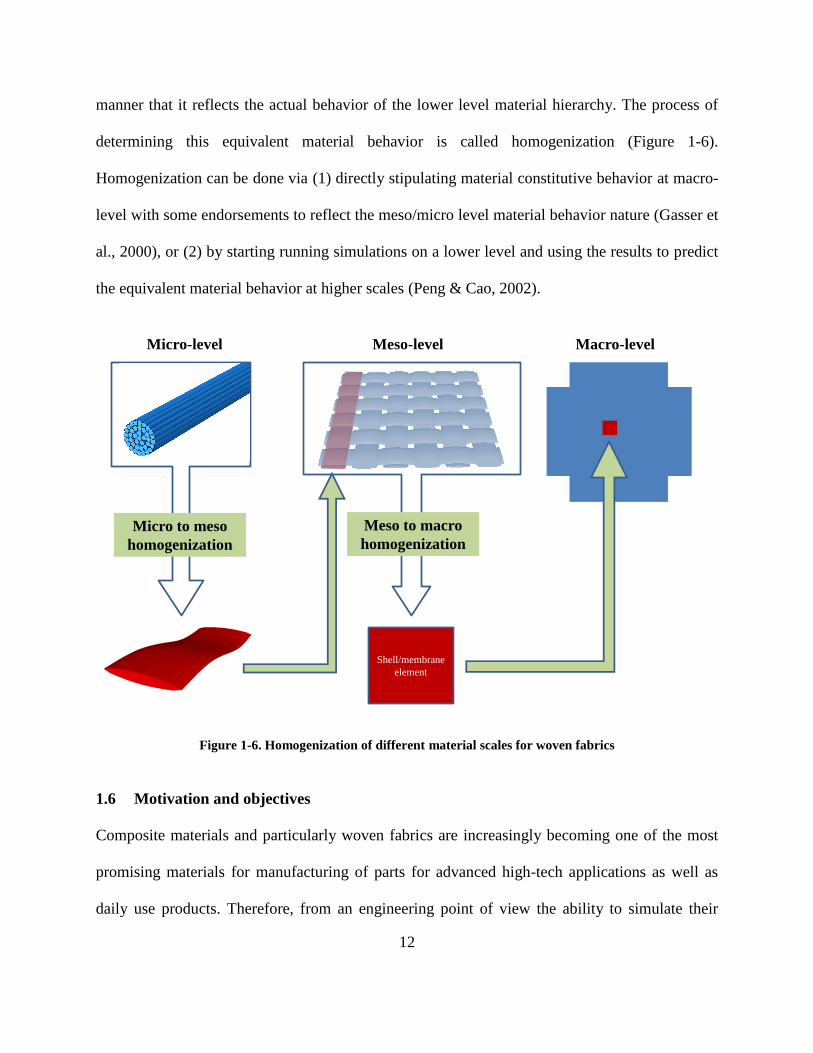
manner that it reflects the actual behavior of the lower level material hierarchy. The process of
determining this equivalent material behavior is called homogenization (Figure 1-6).
Homogenization can be done via (1) directly stipulating material constitutive behavior at macro-
level with some endorsements to reflect the meso/micro level material behavior nature (Gasser et
al., 2000), or (2) by starting running simulations on a lower level and using the results to predict
the equivalent material behavior at higher scales (Peng & Cao, 2002).
Figure 1-6. Homogenization of different material scales for woven fabrics
1.6 Motivation and objectives
Composite materials and particularly woven fabrics are increasingly becoming one of the most
promising materials for manufacturing of parts for advanced high-tech applications as well as
daily use products. Therefore, from an engineering point of view the ability to simulate their
Shell/membrane
element
Micro to meso
homogenization
Meso to macro
homogenization
Micro-level Meso-level Macro-level

13
forming process and performance during service is of crucial significance. Although there has
been a vast amount of research and development in academia as well as industries on these
materials, there remain a number of challenges in terms of realistic simulation of fabrics forming
processes. These challenges are mostly due to the multi-scale nature of woven fabrics which can
not be considered in the conventional numerical simulation packages. Recently, some well-
known developers of Computer Aided Engineering (CAE) tools such as SIMULIA™ and ESI™
have devoted particular numerical functionalities for dry woven fabrics in their software
packages (Abaqus® and PAM-FORM
®, respectively). Nonetheless, there are complex
phenomena that limit full characterization and implementation of these materials. An important
one which has been argued to be of high importance in fabric simulation is the interactions
between tension along yarns (warp and weft direction) and the fabric shear rigidity (resistance to
change in angle between weft and warp yarns, also known as trellising). Although in the past for
the sake of simplicity it was assumed these two deformation modes are decoupled (Xue et al.,
2003; Yu et al., 2002), it has recently been proven by researchers (Launay et al., 2007; Cavallaro
et al., 2004; Komeili and Milani, 2011) that this might not be true for all applications. This proof
has been achieved by using numerical simulations and homogenization (Komeili & Milani,
2011) as well as experimental techniques (Cavallaro et al., 2004; Launay et al., 2007; Willems et
al., 2008a). Therefore, new research projects have been initiated by different groups to study this
coupling effect in more details and include it in numerical simulations of fabrics (Harrison et al.,
2012; Lee et al., 2009a; Lee et al., 2009b). However, there still exists a lack of knowledge in
terms of full characterization and standardization of test methods and fixtures for these materials.
As a result, the following specific objectives are defined for this thesis:

14
1. From fundamental materials science perspective, the first objective is to explore possible
methods for full characterization of shear-tension interaction in woven fabrics. Two
general approaches will be sought: (1) design and manufacture of new test fixtures for
direct experimental characterization; (2) numerical simulations of fabric unit cells at
meso-level followed by the application of homogenization techniques for extracting a
macro-level shell model.
2. To show the application of above methods, as a case study, the second objective includes
performing a full in-plane characterization of a typical TWINTEX plain-weave. In
particular, the virtual experimentation technique will be focused on for this
characterization and new closed-form polynomial functions representing the in-plane
behavior of the fabric will be extracted.
3. From an application perspective, the third objective is aimed at studying the effect of the
characterized shear-tension interaction in predicting mechanical behavior of fabrics in
different applications. Namely, effects of shear-tension coupling during the analysis of
twisting resistance in woven fabric inflatable structures, as well as in a set of stamp
forming simulations via a hemispherical mold shape, a benchmark double dome shape
(Willems et al., 2008b), and a tetrahedral shape are to be discussed.
1.7 Thesis outline
This thesis is composed of 7 chapters and 3 appendices. Chapter 2 discusses a synopsis of past
research conducted on the characterization and modeling of woven fabrics and their forming
studies and simulations. Chapter 3 presents current approaches on the simulation of woven
fabrics at macro-level and non-orthogonal behavior of woven fabrics. Chapter 4 discusses the

15
currently conventional experimental methods for characterization of woven fabrics as well as
some fundamental discussions for using their data in establishing a reliable macro-level fabric
model. It also outlines the missing point of data that are required for macro-level models. As a
suggested solution, it introduces a new test fixture designed and manufactured by the author and
colleagues. Chapter 5 is devoted to developing a meso-level FE model for the TWINTEX plain
weave fabric. It includes a multi-objective inverse identification to obtain yarn properties of the
fabric, which in turn will be used in Chapter 6 to run virtual experiments on the material for a
full characterization under general in-plane loading conditions (tension + shear). Viability of
running virtual tests using the FE method is discussed and tested in Chapter 5. Chapter 6
includes extraction of the material’s stress response surfaces via virtual experiments on the
characterized meso-level fabric model. Then the results are used to study the response of
TWINTEX inflatable beams using classical mechanics of materials, and forming processes using
a macro-level constitutive material model implemented into a non-orthogonal fabric material
model in Abaqus VFABRIC subroutine. Comparisons are made between results of the new
model and earlier model by ignoring the shear-tension coupling terms. Finally, Chapter 7
includes a summary of the work and overall discussions, conclusions and plans for future work.
The appendices include the FORTRAN subroutines developed for implementing the meso-level
model in Abaqus including the yarn material constitutive model and boundary/kinematic
conditions (Appendix A), details of matrix transformations used for the meso-level yarn model
(Appendix B) and the macro-level non-orthogonal model for fabric material model of Abaqus
(Appendix C). Figure 1-7 illustrates the summary of topics discussed in each chapter.

16
Figure 1-7. Outline of the topics discussed in each chapter
17
Chapter 2: Background
This chapter presents the past and current state of the research conducted on analyzing the
mechanical behavior of woven fabrics. This includes efforts for characterization of fabrics’
mechanical behavior, proposed models and simulation techniques.
2.1 Mechanical behavior of woven fabrics
Textile manufacturing is one of the oldest industries that roots in the dawn of human civilization.
Therefore, embedding of reinforcements in the form of textiles into the matrix materials has first
benefited from textile industries in terms of manufacturing preforms with complex geometries,
and second from the analytical and experimental techniques used for characterization of cloth
fabrics (Long, 2006). Most of the early attempts in characterization of woven fabrics for
applications in composite materials are rooted in the techniques that were already developed with
textiles in apparel industries. Haas and Dietzius (1918) studied the mechanical behavior of
woven fabrics used for balloons and airships. Their analytical methods were developed based on
stress equilibrium and incorporated rudimentary models of meso-level yarns. Peirce (1937)
presented extended versions of geometrical models for meso-level yarns for apparel industries.
Moreover, numerous experimental works has been done on different aspects of woven fabrics
including: tension (Freeston et al., 1967; Grosberg & Kedia, 1966), in-plane shear (Grosberg et
al., 1968; Grosberg & Park, 1966; Spivak & Treloar, 1967, 1968; Spivak, 1966), bending
(Abbott et al., 1971; Grosberg & Swani, 1966a; Grosberg, 1966) and buckling (Grosberg and
Swani, 1966b). However, these results were more qualitative and descriptive, and lacked the
details to be incorporated into general purpose, accurate numerical simulations. Kawabata et al.
(1973a, 1973b, 1973c) introduced a set of mechanical models describing the non-linear stress-

18
strain relations for woven fabrics and later suggested comprehensive tests on fabrics called KES
(Kawabata Evaluation System) which enabled an accurate and reproducible measurement of
fabric low-stress mechanical properties (Hu, 2004). Kawabata fabric model includes a set of
truss elements representing yarns and stiffness elements for interaction between yarns (Figure 2-
1). KES set of experiments can be conducted to extract the material constants for this model
(Chou and Ko, 1989). However, this model is a simplification of geometrical and mechanical
system of the total fabric and also the full characterization of its parameters urges the high cost
of experimental setups (Hu, 2004).
Figure 2-1. Kawabata model for meso-level modeling of plain woven fabrics
With the advancement of computational techniques and digital computers, numerical methods
found more and more attraction in the field of structural composites. Among different numerical
techniques, Finite Element Method (FE/FEM) appeared to be the most promising technique. The
first attempt for studying fabrics using FE method was on consolidated textile composites
(Whitcomb, 1989; Whitcomb et al., 1995). However, studies on the dry fabrics in meso-level
simulations of yarns (Gasser et al., 2000; Page & Wang, 2002; Peng & Cao, 2002; Peng & Cao,
Warp
(X1)Weft
(X2)
(X3)
Warp
(X1)Weft
(X2)
(X3)
1D stiffness elements

19
2000) as well as macro-level simulation of fabrics (Boisse et al., 1997; Collier et al., 1991; Lucas
& Pickett, 1998) started to grow fast in the last few decades. Soon the conventional techniques
for finite element analysis proved to be inefficient due to multi-scale nature of woven fabrics
and, hence, modifications into finite element procedures were suggested by different researchers
both in meso-level (Badel et al., 2009; Badel et al., 2007, 2008) and macro-level (Peng & Cao,
2005; Xue et al., 2003; Yu et al., 2002) modeling.
2.2 Draping and forming simulation of woven fabrics
Simulation of fabrics in macro-level can have different applications; for instance in clothing,
fashion and apparel industries (Hu, 2004), computer graphics for animation and games (Breen et
al., 1992), modeling of automotive airbag deployment (Zacharski, 2010), and inflatable
structures (Cavallaro et al., 2006). The purpose of simulation in forming process of woven
fabrics can have multiple notions including but not limited to:
1- Calculating the permeability of a preform in order to simulate the resin injection process
(Loix et al., 2008; Verpoest & Lomov, 2005)
2- To find the properties such as volume fraction, fiber direction etc. in the final composite
part (Long, 2006)
3- Detection of failure modes such as yarn breakage that may happen during manufacturing
(Pickett, 2002) as well as wrinkles developed in fabrics (Zouari et al., 2006).
4- Prediction of ply template and stacking for net-shape forming (Long, 2006).
Although draping and forming simulations are often used interchangeably, it can be said that
forming is a more general term and not all the forming processes involve draping. In the field of
clothing textiles as well as textile composites, draping in its basic meaning is defined as the

20
ability of a fabric to cover a 3D shape under its own weight (Hu, 2004; Strong, 2008). Whereas
forming can be assisted with external forces such as punch and holders (Boisse, 2006).
“Draping” is more common for fabrics in fashion and computer graphics (Breen et al., 1992; Hu,
2004). Thermo-stamping and some other forming techniques are more common for structural
fabrics, where there is a considerable external force from punch and blank-holder. The following
sections will review some of the most common simulation techniques in the latter area.
Nonetheless, there are some techniques for quantitatively studying the general formability of
fabrics. For example Yu et al. (1994) studied the mechanical properties of selected fabric
materials and subsequently by running a forming process on the same fabrics (Cai et al., 1994)
correlated test data and arrived at a formability index which can qualitatively show the
formability of fabrics. However, this assumes a comparison between fabrics under identical
forming condition and is not able to provide designers with details of the formed fabric in the
final part such as updated fiber orientation.
2.2.1 Geometrical models
Geometrical models (also known as mapping approaches) are based on mapping the geometry of
the fabric piece to the shape of the draping object or forming die. Basically, geometrical models
are based on assumptions that ignore the mechanical properties of fabrics and tool-part
interactions. The most simple case can be the assumption of in-extensible yarns in a pin-joint
fisher man network and fitting this network around a 3D shape (Potter, 1979; Robertson et al.,
1981; Van West et al., 1991). Pin-joints are located at the cross-over points of yarns and yarns
are free to rotate. It is also possible to include the coherent slippage of yarns induced at cross-
over points where the yarns are interlaced (Potter, 1979). However, the geometrical methods

21
need introducing an initial point (or direction of warp and weft) to start constructing the rest of
the fabric mapping, whose selection can greatly affect the final outcome of the model (Long,
2006). Moreover, it does not take into account the mechanical resistance and response of the
fabric (or its interaction with the tool) which means fabric is free to deform. Van Der Weeen
(1991) tried to improve the latter limitation by bringing the concept of general energy required
for draping the fabric around 3D shape and minimizing this total energy through iterations.
Geometrical techniques can be effectively used for hand layup simulations and optimization
(Hancock and Potter, 2006). Moreover, they are fast and easy to implement and therefore
recently some commercial CAD (Computer Aided Design) packages started incorporating them.
However, the fact that they ignore the mechanical conditions and tool-part interactions, which
can play a significant role for automated manufacturing process, makes these tools limited
especially for parts with asymmetric shapes (Long, 2006). Therefore, the need for models which
can include the mechanical constitutive behavior, boundary conditions and tool-part interactions
was imminent. Essentially, there are three commonly known techniques which incorporate these
aspects, (1) discrete; (2) semi-discrete; and (3) continuous (also known as constitutive) models
(Boisse et al., 2008; Boisse, 2010), which are discussed as follows.
2.2.2 Discrete models
Multi-scale nature of woven fabrics inherently suggests using a model that includes the
heterogeneity of fabrics up to the meso-level or even micro-level. Although originally this
seemed to be an ambitious plan, successful efforts were made and included the geometrical
features of lower scales into the macro-level simulations. Ballhause et al. (2005, 2006) developed
a discrete model based on the 1D (translational and rotational) stiffness elements with dynamic

22
(inertia) effects. This model was very close to Kawabata’s model (1973a, 1973b, 1973c) and was
successfully implemented into an explicit finite element package in order to simulate basic
deformation modes such as bias-extension and shear/picture frame test (these tests will be
discussed in more details in Chapter 4). Figure 2-2a shows the results of their simulation for
shear frame test. As it can be seen, the phenomenon like fabric wrinkling has been captured by
this method. Later on, Benboubaker et al. (2007) used a similar model for the simulation of
fabric draping. In order to make the simulation physically closer to reality, research projects were
performed to model yarns with shell elements instead of 1D stiffness elements (Boisse et al.,
2011; Gatouillat et al., 2010) or even using full 3D elements to mesh the fibrous yarns (Tavana et
al., 2012). These two approaches are depicted in Figure 2-2(b and c).

23
Figure 2-2. Discrete models for studying fabric deformation; (a) yarns are modeled by 1D stiffness
(translational and rotational spring) elements (Ballhause et al., 2006); (b) yarns are modeled by shell elements
(Gatouillat et al., 2010); (c) yarns are modeled by solid elements (Tavana et al., 2012)
24
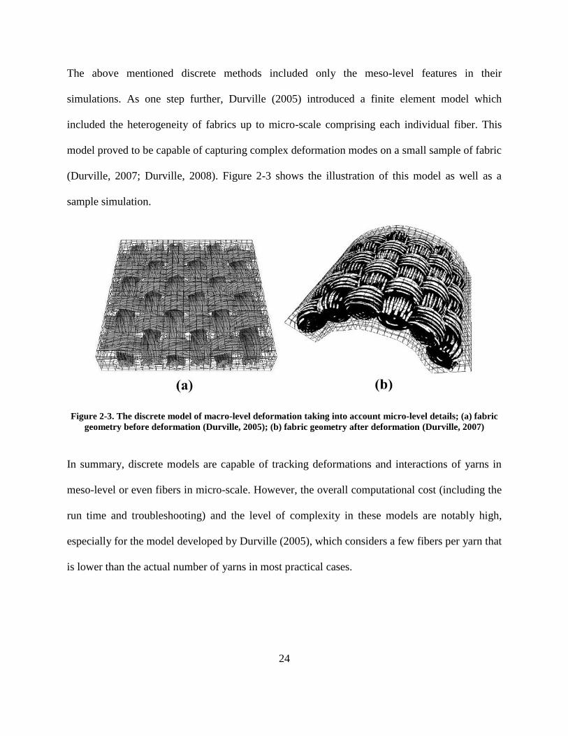
The above mentioned discrete methods included only the meso-level features in their
simulations. As one step further, Durville (2005) introduced a finite element model which
included the heterogeneity of fabrics up to micro-scale comprising each individual fiber. This
model proved to be capable of capturing complex deformation modes on a small sample of fabric
(Durville, 2007; Durville, 2008). Figure 2-3 shows the illustration of this model as well as a
sample simulation.
Figure 2-3. The discrete model of macro-level deformation taking into account micro-level details; (a) fabric
geometry before deformation (Durville, 2005); (b) fabric geometry after deformation (Durville, 2007)
In summary, discrete models are capable of tracking deformations and interactions of yarns in
meso-level or even fibers in micro-scale. However, the overall computational cost (including the
run time and troubleshooting) and the level of complexity in these models are notably high,
especially for the model developed by Durville (2005), which considers a few fibers per yarn that
is lower than the actual number of yarns in most practical cases.

25
2.2.3 Semi-discrete models
These models are again rooted in the multi-scale nature of woven fabrics. The basic idea is to
develop a customized macro-scale element which can be used in regular finite element packages,
while embedding some features of multi-scale nature of fabrics (meso-level yarns in this case).
In other words, each element in a macro-level finite element mesh represents a number of unit
cells of the meso-level woven fabric (Figure 2-4).
Figure 2-4. The bilinear element in a semi-discrete model (Boisse, 2006)
The deformation energy from different loading modes on these unit cells are the basis for
formulating the finite element solver. For example, in virtual displacement field of , the virtual
work theorem can be expressed as (Hamila et al., 2009):
( ) ( ) ( ) (2.1)
where , and are virtual works done by external forces, internal energy storage and
acceleration, respectively. The first and the last terms are similar to the ones for regular elements
and can be calculated as (Boisse et al., 2001):

26
( ) ∫
∫
(2.2)
( ) ∫
(2.3)
In which and are the body forces on the domain (element) and reaction forces on the
traction boundary, is the domain and is the traction boundary. Note that for
displacement boundary conditions ( ) to comply with the weak form formulation in finite
element (Fish and Belytschko, 2007).
Extraction of ( ) for homogeneous materials is a function of stress and strain integrated
over the entire domain (Holzapfel, 2000), however, for the heterogonous woven fabrics it can be
decomposed as energies stored by tension in warp and weft ( ( )), trellising shear between
warp and weft ( ( )) and bending moment of the fabrics (
( )). The calculation of total
and each virtual work component can be done via (Hamila et al., 2009):
( ) ( )
( ) ( ) (2.4)
( ) ∑
( )
( )
(2.5)
( ) ∑ ( )
(2.6)
( ) ∑
( )
( )
(2.7)

27
is the total number of unit cells in the fabrics which are embedded in the macro-level
element and is the index referring to each individual cell, ( ) and
( ) are the virtual
axial strains and virtual curvatures in warp and weft directions, respectively, and ( ) is the
virtual angle change between yarns. Similarly, ,
and are the axial tensions,
bending moments along warp and weft direction, and in-plane shear moment. and are the
length of the element along warp and weft directions, respectively. Figure 2-5 depicts the
superposition of these different loads on a sample fabric unit cell.
Figure 2-5. Semi-discrete model; (a) the selected unit cell of the fabrics and applied loads, note that ii
subscript is used instead of i for 1 and 2 (Hamila et al., 2009); (b) loads on the unit cell in decoupled form
shown in 3D (Allaoui et al., 2011)

28
The level of complexity/details of energy function and the whole analysis can be adjusted by
adding or removing details in the ( ) function (Eq. 2.4). For instance, Boisse et al. (2001,
1997) only included the axial tension terms in the total energy function ( ( ) ( )),
whereas Badel et al. (2008, 2005) and Zouari et al. (2006) added the effect of in-plane shear
( ( ) ( )
( )), and Hamila et al. (2009, 2011) additionally included the effect
of bending (Eq. 2.4). Moreover, the three-node triangular element with this formulation was also
developed (Boisse et al., 2008; Hamila & Boisse, 2008; Hamila & Boisse, 2007) and helped
increasing the flexibility of fabric meshing. While no interaction is assumed between loading
modes in the above formulation, a similar method was used to investigate deformation of textile
fabric composites with interactions (Milani and Nemes, 2004). In the latter study different
energy terms were used for reinforcement and matrix, and it was proven that adding an extra
term which includes the interaction between these two energy terms can increase the prediction
accuracy noticeably.
Results of the worked reviewed in the last paragraph prove that the semi-discrete method is
capable of capturing a realistic macro-level behavior of fabrics and their forming processes.
Moreover, compared to the (fully) discrete method, semi-discrete modeling requires less
computational time. On the other hand, this method needs an augmentation (e.g., UEL as a
FORTRAN subroutine for Abaqus) of finite element codes in a high level which may not be easy
to implement in all finite element packages and/or to assure its convergence.
2.2.4 Continuous models
These models are the most convenient option in terms of implementation into a finite element
package and minimizing the computational cost. Regular shell/membrane elements can be used

29
in these models for meshing fabrics. However, considerations are kept in mind to mimic the
meso-level structure of fabrics and direction of yarns. Changes to material properties and
defining two material directions along warp and weft are among the most important factors to be
taken into account. Moreover, modifications on the orientation of elements during meshing
should be applied to avoid element shear locking during simulations (Yu et al., 2006).
The continuous models are currently the most popular candidates in simulation of forming
processes (Boisse, 2010; Long, 2006) as well as other applications such as impact modeling of
fabrics in the bullet-proof armour systems made of woven fabrics (Shahkarami & Vaziri, 2007;
Shahkarami & Vaziri, 2006; Shahkarami, 2006). This is because of the fact that in these models
only the constitutive material properties of the shell/membrane element needs to be defined in
order to reflect the actual meso-level yarns. Considering the orthogonal arrangement of fibers
prior to loading, orthogonal constitute material models might be the first choice (Dong et al.,
2000). However, keeping track of the deformation and yarn directions in the fabric raises the
need for a non-orthogonal formulation (Xue et al., 2003; Yu et al., 2002). Moreover, focusing
solely on the material constitutive behavior brings the possibility of exploring different options
for the material behavior such as hypo-elastic or hyper-elastic material models (Boisse, 2010;
Milani & Nemes, 2004).
2.3 Summary
A literature review was conducted on the previous efforts in proposed models for the simulation
of woven fabrics. Different approaches to the problem were presented and discussed. As
mentioned earlier, the main goal of this chapter was reviewing different approaches in forming
and draping simulation of woven fabrics, whereas the ultimate aim of the thesis is on enhancing

30
the fabric material constitutive modeling for forming simulations using shell models. Therefore,
more details about the continuous shell models along with their mechanical formulations will be
discussed in the next chapter.

31
Chapter 3: Fundamentals of macro-level fabric simulation using continuous
models
This chapter discusses the principles of shell elements formulation and also their adaptation for
finite element modeling of fabrics. The non-orthogonal aspect of material behavior which
represents the meso-level structure of fabrics (yarns) is elaborated on and the “fabric” material
model developed as a built-in module in Abaqus is discussed.
3.1 Thin-shell structures
The analytical solution of fabrics under simple and basic deformation modes such as uni-axial
tension and shear can be achieved via simple continuum mechanics formulations. However, for
complex deformations such as forming process on a 3D die and punch, this is not possible.
Therefore, finite element analysis along with the discretization of fabric domain is the preferred
method. As mentioned in the previous chapter, there are notable contributions from earlier
studies suggesting to incorporate a new formulation for elements that are used in this type of
simulations (Hamila & Boisse, 2008). However, in order to avoid the challenge of developing a
new formulation and the issues related to its implementation (convergence), it has also been
suggested to use the conventional available elements with modified material formulations
(Boisse, 2010). In the latter approach depending on the type of deformation to be studied, 2D
plane stress (Peng & Cao, 2005), membrane, and shell (Long, 2006) elements are used. Note that
the main difference between membrane and shell elements is neglecting the bending moment in
the material. Although this bending moment is quite small in dry woven fabrics, there are

32
evidences that it can affect the simulation results in particular cases (Hamila et al., 2009).
Standard shell elements are selected in this research as the preferred type of FE elements.
3.2 Modeling of shells
Generally, a continuum media can be simplified as a shell if the length-to-thickness and width-
to-thickness ratios are high (Timoshenko and Woinowsky-Krieger, 1959). There are different
suggestions for the minimum value on this ratio, but the rule of thumb is a value between 10 or
20. In this case the through thickness strains of the shell can be neglected and its deformation is
summarized as a combination of in-plane deformations (tension and shear) and flexural bending.
The principles of shell deformation and the general theory behind it can be found in textbooks
and other studies (Kaw, 1997; Timoshenko and Woinowsky-Krieger, 1959). It must be
mentioned that in general, shells and plates are two entities with similar mathematical
assumptions for material structural behavior where shell is more general by allowing an initial
curvature. In order to provide the reader with a general idea about the shell theory, derivation of
formulation for a flat shell is briefly discussed below.
Using the basic equations of continuum mechanics (i.e., equilibrium, deformation relations, and
constitutive behavior), the following matrix equations for a shell can be written (Chou and Ko,
1989):
[
] [
] [
] (3.1)
Assuming x3 is the direction normal to the plane (direction 3 in Figure 3.1):
∫
(3.2)
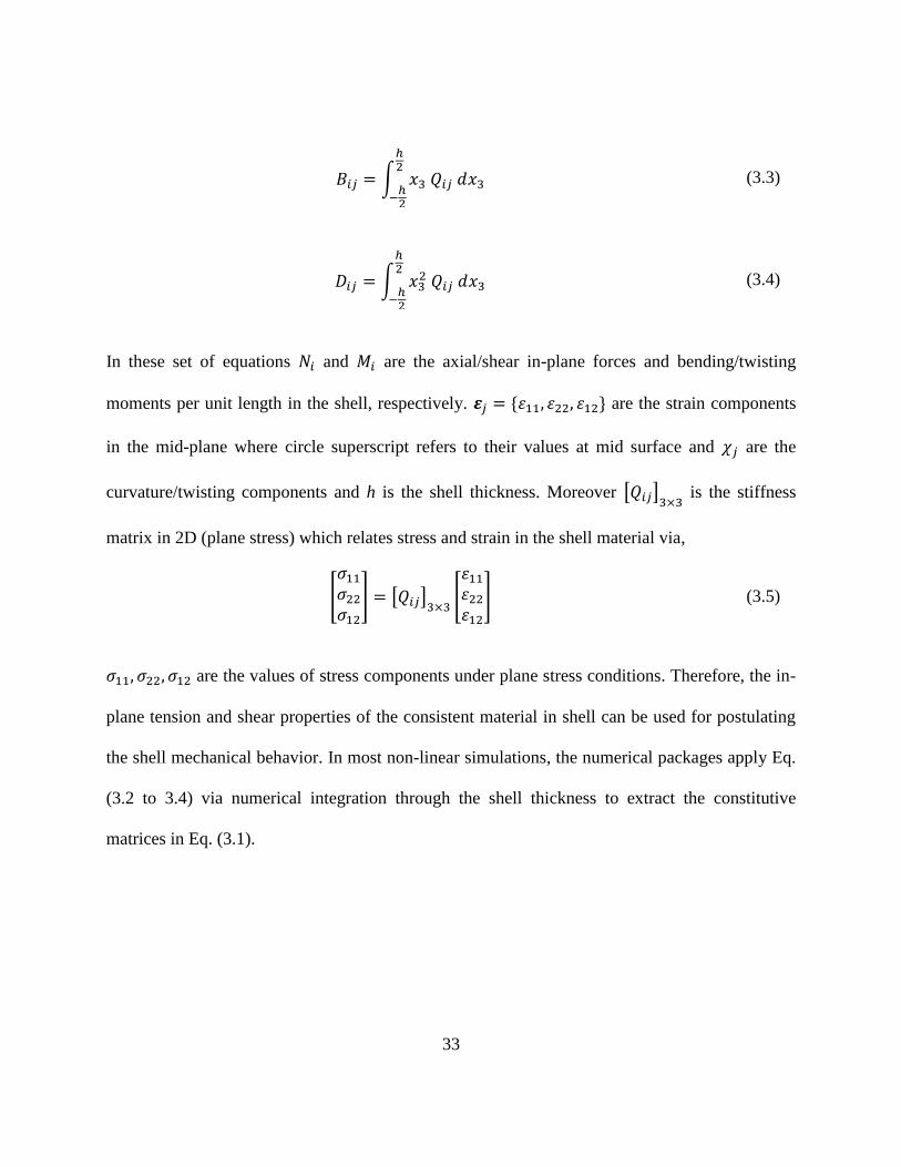
33
∫
(3.3)
∫
(3.4)
In these set of equations and are the axial/shear in-plane forces and bending/twisting
moments per unit length in the shell, respectively. are the strain components
in the mid-plane where circle superscript refers to their values at mid surface and are the
curvature/twisting components and h is the shell thickness. Moreover [ ] is the stiffness
matrix in 2D (plane stress) which relates stress and strain in the shell material via,
[
] [ ] [
] (3.5)
are the values of stress components under plane stress conditions. Therefore, the in-
plane tension and shear properties of the consistent material in shell can be used for postulating
the shell mechanical behavior. In most non-linear simulations, the numerical packages apply Eq.
(3.2 to 3.4) via numerical integration through the shell thickness to extract the constitutive
matrices in Eq. (3.1).

34
Figure 3-1. The basic loading modes on a shell: (a) in-plane modes; (b) bending modes
3.3 Shell models used in Abaqus
SIMULIA Abaqus is the FE package employed in this study. It offers a broad library of shell
elements suitable for different structural applications. The element type used is S4 (and its
closely related element with reduced integration S4R) which allows the modeling of curved
surfaces, exhibits nonlinear material response and undergoes large overall deformations
(SIMULIA, 2010). The formulation of the stiffness matrix in this shell element is a modified
version of Equations (3.1) to (3.5), in order to take into account the effects of surface curvature.
(a)
(b)
1
2
3
N1
N1
N2
N2
N12
N12
N12
N12
M1
M2
M2
M1
M12
M12
M12
M12

35
As it can be seen from the Equation (3.5), the formulation of shell to extract the stiffness matrix
for FE needs the constitutive behavior of the material. In general, the in-plane and transverse
material properties are required to be extracted from mechanical tests. However, measuring the
transverse shear stiffness of dry fabrics is not easy. On the other hand, the effect from this
transverse stuffiness is of secondary importance compared to the in-plane stiffness values that
directly lead to bending stiffness. Moreover, it is shown that the shear stiffness of fabrics is very
low in the dry form and using a small shear value for stability and accuracy of numerical
methods is sufficient (Boisse et al., 2005). Therefore, the main issue is the characterization of in-
plane material properties. The material models available for this purpose are discussed in the
following. Abaqus software has a built-in procedure for estimating the transverse shear stiffness
of the shell elements by matching the shear response for the shell to that of a 3D solid under
bending about one axis (SIMULIA, 2010). However, this capability is not available for elements
with user-defined (FORTRAN subroutine) material properties. In this case, consulting the
software’s documentation, it is suggested to use transverse shear stiffness calculated from
following relationships:
(3.6)
where and are the shear moduli in the out-of-plane directions. These estimations have
been commonly used in simulation of fabric forming processes (Lee et al., 2009).
3.4 In-plane elastic material model for dry fabrics
As mentioned before, dry fabrics are constituted from two main structural directions (warp and
weft). It has been proven that proper modeling of woven fabrics requires tracking of these two

36
structural directions and defining the material stress response based on updated yarn directions
(Peng & Cao, 2005; Xue et al., 2003). General purpose shell elements in a FE code are
formulated based on the stress and strain increments in an orthogonal coordinate system as
follows:
{
} [ ] {
} (3.7)
In which [ ] is the stiffness matrix of the material in the shell element under plane stress
condition. However, the material properties for the fabric with respect to the warp and weft
structural directions (i.e., in fabric local coordinates and shown in Figure 3-2) is written as
(Peng & Cao, 2005):
{
} [ ]
{
} (3.8)
where and are the stress rates in the contravariant and strain rates in the covariant
coordinate systems that are based on warp and weft directions as shown in Figure 3-2, and [ ] is
the material constitutive matrix which relates the latter stress and strain rates. According to the
continuum mechanics formulation (Peng & Cao, 2005),
(3.9)
(3.10)
, and ( ) are the base unit vectors for orthogonal, non-orthogonal covariant and
contravariant (local) coordinate systems, respectively. The relation between covariant and
contravariant coordinate systems base vectors is (Ogden, 1997):

37
(3.11)
where is the Kronecker delta. Figure 3-2 schematically shows the covariant coordinate
system and corresponding contravariant system which can be found through the equation above.
Having that, the P matrix can be defined with respect to (warp rotation) and (relative angle
shear) angles (Figure 3.2) as:
[
( ) ( )
] (3.12)
Figure 3-2. Coordinate systems used for simulating the deformation of woven fabrics; (a) orthogonal
coordinate systems before deformation; (b) non-orthogonal covariant (along yarns) and contravariant
coordinate system after deformation
Expanding this formulation for stress-strain constitutive equation, Peng and Cao (2005)
concluded that a proper form of transformation matrix from the non-orthogonal coordinate
system of fabric (Equation 3.8) to the orthogonal coordinate system of the shell element
(Equation 3.7) can be found as:

38
[ ] [ ] [ ][ ] (3.13)
[ ]
[
( ) ( ) ( ) ( )
( ) ( ) ( ) ( )
( ) ( ) ( ) ( )
( ) ]
(3.14)
This transformation can be incorporated into Abaqus via user-defined material FORTRAN
subroutines such as UMAT (for Abaqus/Standard) and VUMAT (for Abaqus/Explicit).
3.5 Built-in fabric material model of Abaqus
Due to recent popularity of non-orthogonal material models for fabrics, Abaqus has developed a
new built-in material model in its recent releases, hence removing the need for UMAT or
VUMAT implementation of Eq. (3.14). This anisotropic nonlinear fabric model is capable of
tracking the direction of warp and weft yarns and defining the material response based on the
updated directions and the relative shear angle (trellising). The inputs needed to use this material
model include fabrics nominal stresses along warp and weft ( and , respectively) as a
function of nominal strains, and nominal shear stress ( ) as a function of shear angle between
yarns, . The relation between the warp and weft material stress values and the shell element
Cauchy stresses which is used by the FE code is given as (SIMULIA, 2010):
( ) ( ) ( )(
) (3.15)
In which, is the volumetric Jacobian (Mase and Mase, 1999), are the in-plane stretch values
along warp and weft, respectively.

39
3.5.1 FORTRAN subroutine for fabric material model of Abaqus
As mentioned in Section 3.5, the current built-in fabric material model in Abaqus calculates the
stress in warp and weft directions only as function of their respective strains and the biaxial
effect and/or axial-shear interaction is not included. Similarly, shear stress is also only calculated
as a function of shear angle. However, Abaqus provides the user with the ability to define a
customized material response for fabrics. The FORTRAN subroutine, VFABRIC, is specified for
this purpose. The inputs needed for this subroutine include local strain values (warp, weft and
shear angle), increment in strains and some other variables that might be required in particular
models (e.g., temperature and user defined field variables). The output is the updated stress
value, but additional parameters can also be added (e.g., customized state variables). According
to the author’s experience, this model has a better numerical stability for non-orthogonal material
behavior compared to a general purpose UMAT or VUMAT subroutine. Therefore, the fabric
material model of Abaqus along with its related subroutine (VFABRIC) is used in subsequent
chapters for the FE modeling exercise at macro-level.
3.6 Summary
Macro-level modeling for studying deformation of woven fabrics was reviewed by starting from
a general plate/shell model. The non-orthogonal material behavior formulation of fabrics is then
discussed and the built-in material model of Abaqus (fabric which can be customized via vfabric
subroutine) was introduced.

40
Chapter 4: Conducted experimental characterization techniques
Recalling the experimental part of objectives of this thesis (Section 1.6 and Figure 1-7), in this
chapter results of measurements on uni-axial tension response and shear frame response of the
TWINTEX® fabric are presented. Next, arguments on the presence of dependency of the shear
response to the axial tension along yarns are provided and an experimental procedure is
suggested for its full characterization. Accordingly, a new test fixture designed and manufactured
by the author and collaborating research groups is presented and discussed.
4.1 Importance of experimental data and formulations
Every engineering analysis including numerical simulation of fabrics requires a set of input data
in the form of postulated equations and constants. These equations and constants are to
approximate the true nature of the material as it is observed in experiments. In other words,
besides all the principles that are based on theory (e.g., conservation of mass and energy), there
should be actual numbers (model constants) that can represent the given material behavior (e.g.,
Young modulus and Poisson’s ratio). Calculation of stress, strain and material deformation can
be done via continuum mechanics theories and mathematical methods (Mase and Mase, 1999).
However, the relationship between stress and strain values, for instance, is not something that
can be quantified easily. This relationship needs experimental data. Often, postulating
experimental equations with a set of constants are used in order to represent the properties and
response of materials close to what is observed in experiments.
In the case of dry fabrics, the multi-scale nature of these materials, non-orthogonal, anisotropic
and non-linearity of the response are amongst factors that make experimentation particularly
different from that of, e.g., homogeneous metals and polymers. The fact that dry fabric materials

41
are made of two main structural directions along yarns and the main deformation mode during
forming is the trellising shear (the change in the angle between yarns), suggests that studying the
axial (uni-axial and biaxial) response as well as shear response can be a good measure of fabric
deformation (Peng & Cao, 2005; Xue et al., 2003). This was ideally based on the assumption that
these two deformation modes do not have interactions with each other. As it will be shown later,
this assumption has recently been proven to be not valid and therefore extended studies on
characterizing the level of interaction between shear and tension in fabric is required.
4.2 Fabric material
The fabric used in this study is made of yarns with comingled fibers of E-glass and
Polypropylene (PP). The product is commercially known as TWINTEX® and is produced by
Fiber Glass Industries (FGI). The industrial code for the material, TWINTEX® TPP60N22P-060
which signifies a TWINTEX® material with PP matrix and 60% glass content in weight, woven
in-plane weave architecture. A summary of the material and geometrical parameters of this fabric
is summarized in Table 4-1. An image of the fabric sample along with the yarn spacing (S), yarn
width (w) and yarn height/thickness (h) is depicted in Figure 4-1.

42
Table 4-1. Specifications of the fabric material used in this research, reported by woven fabrics benchmark
forum (http://www.wovencomposites.org)
Parameter Plain weave
Commercial code TWINTEX® TPP60N22P-060
Weight fraction (glass) 60%
Area density (g/ m2) 745
Yarn linear density (tex) 1870
Nominal fiber diameter (µm) 18.5
Nominal thickness, h (mm) 1.0~1.5
Nominal yarn spacing, S (mm) Warp 5.2
Weft 5.2
Nominal yarn width, w (mm) Warp 4.2
Weft 4.2
Figure 4-1. A photo from the fabric samples used in the experiment along with the geometrical features of its
unit cell (spacing, width and thickness)

43
4.3 Uni-axial tension on fabrics
Figure 4-2 shows the configuration of the test fixture as well as the kinematics of the uni-axial
tension on the fabrics. As it can be seen in the figure, a particular type of clamp with corrugated
surface is used to hold the fabric. It was noted from multiple experiments that flat surfaces are
not suitable for running tests on dry fabrics because of sliding. On the other hand, threaded
surfaces for clamping may damage the fibers. Indeed, rubber corrugated surfaces are a common
choice for clamping of woven fabrics that has also been suggested by the producer of the fixture
(Instron®
) and used in custom made fixtures (Willems et al., 2008a).
Figure 4-2. Fixture used for uni-axial tension and the schematic of resulting deformation

44
Although the warp and weft yarns in this type of fabric are made of identical yarns, due to the
underlying mechanisms in weaving and different tensions, bending states. that can induce
damage into the yarns during manufacturing (Chou and Ko, 1989), the fabric responses along
warp and weft may be different at macro-level. Therefore, two separate sets of experiments
needed to be conducted on the fabric along warp and weft.
4.3.1 Conducting the test
Tests are conducted on a universal tension/compression Instron® 5969 (Figure 4-3) machine with
grips demonstrated in Figure 4-2. Unfortunately, currently no widely used standard test method
exists for structural textile fabrics, however, guidelines similar to some standards for clothing
fabrics are selected (ASTM, 2011).
Figure 4-3. Instron 5969 universal tension/compression machine

45
A nominal gage length (distance between nips of grips) of 160 mm was selected with a width of
~62 mm that includes 12 yarns under tension. As recommended by ASTM standard for clothing
fabrics, fabric strips were cut with a higher width and ravelled into the required width. A small
amount of initial tension (less than 1 N/yarn) was applied to the fabric samples to keep it straight
before the test. The moving head of the tensile machine travelled with a constant speed of 0.1
mm/s which is much lower than the speed recommended in the above mentioned ASTM
standard, to avoid any dynamic mass or viscoelastic effects. Five specimens were tested for each
loading case (warp and weft). The raw data representing results of each test on all specimens are
illustrated in Figures 4-4. Strain is estimated from the conventional formula of engineering
strain:
(4.1)
where and are the specimen length before and after loading, respectively. Because the
specimen is uniform between the jaws and the macro-level deformation is small, this
approximation can be a fair measure of the axial strain.

46
Figure 4-4. Response of the fabric to axial tension under five repeats, (a) loading along warp direction; (b)
loading along weft direction
As it can be seen in Figure 4-4 the mechanical response of the material along warp and weft is
relatively different. As discussed before, the reason for this phenomenon can be related to the
fact that although the fabric is nominally manufactured to be balanced along warp and weft,

47
different trends of tension and bending is applied on the yarns during weaving process (Chou and
Ko, 1989) and has resulted in variation of properties along warp and weft. One source that can be
clearly identified and measured is the crimp content along warp and weft. Generally, the
waviness of the interlacing yarns is set by the weave pattern and is referred to as crimp (Long,
2006). The crimp content of a fabric along warp or weft is determined via (Buet-Gautier and
Boisse, 2001):
(4.2)
To do this measurement, one yarn is marked in the fabric and its length is measured ( ).
Then it is meticulously extracted from the fabric and its actual length after straightening is
measured ( ). For the current fabric, five readings of this measurement were done along
warp and weft. Results showed that the average crimp content along the warp direction is 3.37%
whereas the average crimp content along the weft direction is 2.69%. Moreover, the variation of
this crimp content in specimens of each sample group (warp and weft) can be the source of non-
repeatability in reaction forces of the samples as can be seen in Figure 4-4.
Basically, the axial deformation of samples occurs in two stages. First, the waviness of the fabric
is removed and yarns are straightened, then yarns go through axial stretch along their axis. The
reaction forces that are developed in the second stage are considerably higher than the first stage.
On the other hand, a higher crimp content and waviness means a longer straightening stage.
Therefore, recalling Figure 4-4 the outcome of axial tension along warp shows a longer region of
soft material response in the beginning as compared to weft.

48
Next, similar procedures were followed to test tensile behavior of single yarns that were
extracted from warp and weft directions of the plain woven fabric. Figure 4-5 shows a summary
of the experiments on the yarns.
Figure 4-5. Response of the extracted yarns to axial tension, (a) yarns extracted along warp direction; (b)
yarns extracted along weft direction
As it can be seen in Figures 4-5, yarns show repeatable behavior before the failure stage and very
different to the fabric response itself (compare Figure 4-4 and 4-5). The noticeable variations

49
observed in the failure point and post-failure force response curves through repeats of the above
tests is due to the fact that, the effect of material uncertainty plays a more important role in the
failure and fiber breakage compared to the yarn elastic response (initial slope of the curves).
Elastic response would be an average of overall behavior of all fibers inside the yarn whereas the
first breakage depends on the weakest fiber(s) in the yarn. Thus, the observed variation in the
failure point in the force response curves is expected to be more obvious; and also because after
the breakage of few fibers the yarn has a smaller effective cross section, this effect is propagated
into the post-failure regions of the response. To explore the influence of weaving more, effect of
yarns perpendicular to the loading direction was studied by conducting similar procedures on the
ravelled fabrics and comparing them with corresponding results from the fabric. The specimen
was first placed into the grip with a very small amount of pretension (less than 1 N/yarn) to avoid
wrinkles and then the perpendicular yarns were extracted with care (Figure 4-6). The axial
response of raveled fabrics tested along warp and weft are summarized in Figure 4-7.
Figure 4-6. Raveling of the fabric specimen after mounting into the test fixture with small pretension

50
Figure 4-7. Response of the ravelled fabric to axial tension under five repeats, (a) loading along warp
direction; (b) loading along weft direction
An overall comparison among the average values of force response of the original fabric, the
raveled fabric and the yarns are presented in Figure 4-8. As it can be seen, the response that is
extracted from the experiment on single yarns cannot represent the response of the fabric. On the
other hand, the raveled fabrics can be a closer representative of the fabric behavior only for the
weft direction.

51
Figure 4-8. The averaged axial response of the fabric, ravelled fabric and yarns, (a) along warp direction; (b)
along weft direction
4.3.2 Nominal uni-axial response
As mentioned before the purpose of running axial tension tests on the fabric samples is to extract
input data that can represent stress vs. strain response of the material. The result of experiments
in the previous sections showed that although the chosen fabric is supposed to be balanced, it
comprises a somewhat unbalanced behavior along warp and weft. This brings extra complexity

52
in the simulation of material. However, because the focus of the current research is more on the
general methodology and not uncertainty concept, an average of the axial response of the fabric
samples between warp and weft (average response seen in Figure 4-4) in a reasonable strain
range of 0-4% (to avoid failure region) is selected for the following chapters. Figure 4-9
illustrates this nominal response as normalized by the width of the specimen. The reason for
normalizing the force response with the width of the specimen is that the effective parameter in
the axial tension response is the number of yarns that are involved in the tension. Therefore,
normalizing the reaction force by the width of the samples assures comparable values among
different experiments.
Figure 4-9. The nominal axial response of the fabric to axial strain along warp and weft used in the
subsequent models

53
4.4 Shear test on fabrics
Due to low resistance of fabric to the change of angle between yarns (trellising), shear
deformation of woven fabrics is considered as the main deformation mechanism during forming.
Indeed, the low shear resistance is one of the significant reasons for high formability of dry
fabrics. However, unfortunately there is no universal standard method for the characterization of
this shear behavior. One of the first methods used for characterization of fabric shear was based
on Kawabata Evaluation System (KES) which was common at the time for fabrics in apparel
industry (Chou and Ko, 1989; Hu, 2004). However, it has proved to be inefficient for dry fabrics
used in structural composite industries due to a variety of reasons including maximum
achievable shear angle on the fabrics and wrinkling (Bassett et al., 1999) and the non-uniformity
of the deformation (Hu, 2004). Nonetheless, there are two commonly used experimental
techniques which are suggested particularly for structural fabrics in composites research: bias
extension (BE) test (Lebrun et al, 2003; Spivak & Treloar, 1968); and the picture/shear frame
(SF/PF) test (Lussier and Chen, 2002).
4.4.1 Bias extension test
In Bias-Extension test the fabric samples are cut in a rectangular shape with a height-to-width
ratio of 2 or more and fibers with 45° with respect to edges of the rectangle. Then they are loaded
along the length of the rectangular specimen (Figure 4-10a). Applying tension in that direction
forms three different regions as depicted in Figure 4-10b. Ideally the shear angle is
approximately , and 0, in the regions A, B and C, respectively, where (Harrison et al.,
2004):

54
[
√ ( )
√ ]
(4.3)
H and W are the height and width of the specimen, respectively, and d is the displacement of the
moving head in the axial tension machine.
Figure 4-10. (a) Bias extension (BE) test fixture (Peng & Cao, 2005); (b) the schematic of deformation regions;
the ideal shear angle in each regions: C=0, B=γ/2 and A=γ
The advantage of this test is that it is easy to implement because of the simple test setup,
however slippage of the fibers during the test and formation of the above mentioned zones with
fuzzy borders make the interpretation of the test results hard (Zhu et al., 2007a). Moreover, at a
higher range of deformation, significant deviations between theoretically calculated shear angles
at the center (Eq. 4.3) and the actual shear angle have been observed (Harrison et al., 2008). The
Digital Image Correlation (DIC) technique has been used as a solution to this problem by
monitoring the real deformation field that happens in each zone and capturing the true fabric
deformation (Dridi et al., 2012; Zhu et al., 2007a). Nevertheless, the complexity and time of
bringing the image correlation analysis into every experiment and the non-uniform state of

55
deformation in this test make it often hard to interpret the image data straight forwardly (Komeili
& Milani, 2013). A new form of this test called Biaxial Bias Extension (BBE) has been recently
suggested (Abdiwi et al., 2013; Harrison et al., 2012) for the characterization of fabric response
under the influence of initial tension. It is based on applying tension on two sides of the
specimen during the deformation (Figure 4-11). However, this test is not still completely free of
the drawbacks mentioned before for the regular bias extension test.
Figure 4-11. (a) Biaxial bias extension (BBE) test fixture developed by Harrison et al. (2012); (b) the specimen
and ideally distinct deformation zones
4.4.2 Shear/picture frame test
Shear Frame (also known as Picture Frame) test is an alternative to the bias extension test in
order to obtain a closer deformation state to the pure trellis mode. The configuration of a regular
shear frame (SF) test fixture and its schematic are shown in Figure (4-12). Ideally, the kinematics

56
of deformation imposes the required deformation to the specimen in the region of interest (the
rectangular piece in the middle), and this shear deformation can be found via (Long, 2006):
(
√
)
(4.4)
where is the distance between the pins in the frame (side length of the frame).
Figure 4-12. (a) A conventional shear frame test fixture; (b) schematic of the test and resultant deformation
on fabric
Nonetheless, the SF test has a few drawbacks too. First, this particular fixture of the SF test is not
standardized yet and a custom made jig is required. Second, it is very sensitive to mishandling
and specimen alignment. Research on the effect of this phenomenon has shown that

57
misalignment can have a significant impact on the noise in the response (Milani et al., 2007).
Although, modifications are suggested to avoid this difficulty (Lebrun et al., 2003; Milani, et al.,
2009), in practice they are not very effective and may end up in wrinkling which is another
undesired noise source in this test (Zhu et al., 2007b). Finally, although the fixture used in this
experiment does not allow the fabric to directly stretch along yarns, the twisting of yarns during
the shear deformation and the associated meso-level structural deformation result in axial stretch
and subsequently axial stress along the yarns. It has been reported that this indirect yarn
tensioning can affect the shear resistance of the fabrics and the outcome of the test (Launay et al.,
2008; Launay et al., 2007). Moreover, a small amount of initial tension along yarns is required
prior to the shear frame test to reduce wrinkling in the fabrics during the test. Therefore, a
control over this initial tension and its accurate measurement are necessary. A modified test
fixture illustrated in Figure 4-13 (the fixture used in this research) can be used to apply
pretension on the fabric along yarns. Moreover, the image correlation (DIC) techniques can be
implemented to measure the axial strains in the region of interest due to applied pre-tension
(Willems et al., 2008a).
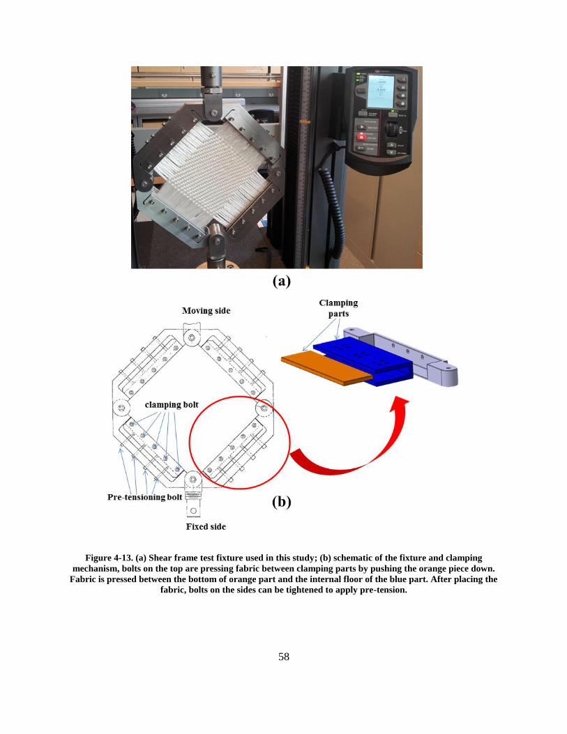
58
Figure 4-13. (a) Shear frame test fixture used in this study; (b) schematic of the fixture and clamping
mechanism, bolts on the top are pressing fabric between clamping parts by pushing the orange piece down.
Fabric is pressed between the bottom of orange part and the internal floor of the blue part. After placing the
fabric, bolts on the sides can be tightened to apply pre-tension.

59
4.4.3 Digital Image Correlation (DIC)
Conventional strain gages have been used for decades to measure and characterize the
deformation of specimens during material testing. However, there are intrinsic deficiencies
associated with them when used on dry fabrics. For example:
Need to have the strain gage attached to the surface of the material; this can induce extra
stiffness in cases that the material is very soft (such as dry fabrics) moreover, there is
always a bonding layer of adhesive between material and strain gage that has its own
problems. Not enough adhesive can result in detachment of strain gage from the surface
and too much adhesive can make the strain gage read deformations in a thick layer of
adhesive instead of specimen.
The gage length in the strain gage is fixed and sometimes too large or too small for the
material of interest. For the dry fabrics where the multi-scale nature of the material can
bring in different scales, this can induce more difficulties; especially if the gage length is
not matching the length of the unit cells. This will make the strain gage to read internal
deformation inside a unit cell which might be different from the macro-level deformation
trend.
The number of strain gages that can be attached to the surface of a material sample is
limited. It is not common to have many strain gages on a small sample. This is both
because of difficulty of adhering them to one sample and also the complexity of
measurement system. Normally for each strain gage a full set of wiring and Wheatstone
bridge (CMH-17, 2012) is required which makes it cumbersome to add more strain
gages.

60
Strain gages are only able to measure the stretch of the specimen along one line. In order
to get better results with more information they are usually placed in particular
arrangements to get strains along at least two to three directions and then data are
combined to get the overall state of deformation (Mase and Mase, 1999). Moreover, they
are not able to distinguish between the out of plane material movement (wrinkles for
example) and tangential deformations on the surface.
One more specific problem associated with strain gages for dry fabrics is that the
adhesive used to attach the strain gage to the sample surface would act like a resin and
after curing consolidates the fabric locally. This will make the region of strain
measurement overly stiff and eventually results in an artifact in data measurement. The
problem becomes worse considering the capillarity of the fibers which soaks a region
larger than the region that was originally wet with adhesive.
All the example problems addressed above suggest the idea of not using traditional strain gages
for testing dry fabrics. Contactless strain gages can be proposed as a potential alternative. Among
different sorts of contactless strain/deformation measurement systems, optical strain gages that
work based on 3D image correlations (Digital Image Correlation, DIC) are shown to be very
promising for the particular type of measurements on dry fabric (Dridi et al., 2012; Lomov, et al.,
2008a; Lomov, et al., 2008b; Willems et al., 2008a).
The basic principle behind the DIC is the stereoscopic vision, which means looking at an object
from two (or more) different viewpoints (cameras). This is similar to the process in human vision
for 3D reconstruction of the images that are received from eyes in brain. Basically, if the relative
distance and angle between cameras are known and they are both looking at the same object
(Figure 4-14), the location of that object can be estimated via certain techniques (DANTEC
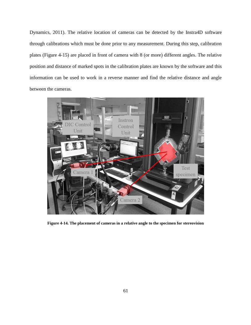
61
Dynamics, 2011). The relative location of cameras can be detected by the Instra4D software
through calibrations which must be done prior to any measurement. During this step, calibration
plates (Figure 4-15) are placed in front of camera with 8 (or more) different angles. The relative
position and distance of marked spots in the calibration plates are known by the software and this
information can be used to work in a reverse manner and find the relative distance and angle
between the cameras.
Figure 4-14. The placement of cameras in a relative angle to the specimen for stereovision

62
Figure 4-15. Three different sizes of calibration plates for the DIC system which can be used for experiments
in different characteristic lengths
By introducing small windows (facets) on the fabric image to refer to a small sub-region of the
surface and locating them in 3D space, the surface of the specimen is reconstructed by the
software. Afterwards, during the deformation, more images are taken from the specimen and
same facets are relocated. By comparing the original position of facets and their current
positions, a discrete deformation gradient matrix is calculated. This deformation gradient matrix
can be used for calculating different strain values. Figure 4-16 demonstrates the grid of facets on
a specimen and the contour of reconstructed surface from viewpoint of left and right cameras.

63
More detailed information on principles of DIC and stereovision can be found in various
references (Bhatti, 2008; Pan et al., 2009; “Q-400 DIC and ISTRA4D training,” 2011).
Figure 4-16. Image processing for calculation of deformation in DIC, images taken from left and right
cameras are shown together; (a) the facets made on the surface of specimen in Instra4D® software; (b) the
reconstructed plane on the surface

64
4.4.4 Preparations for shear frame test
4.4.4.1 Sample sizes
Specimens were cut in the form of a square region with small extended arms as depicted in
Figure 4-17. The region of interest is the square piece of the specimen as shown in the figure.
The regions shown in black are clamped in the shear frame fixture jaws. It was also noted that
extracting one yarn per edge of the region of interest (inner red lines that form the region of
interest rectangle in Figure 4-17) will increase the repeatability of the experimental results by
lowering the change of developing severe wrinkles near the arms.
Figure 4-17. The geometry of specimens used in the shear frame test
4.4.4.2 Preparation of specimens and test fixtures
In the shear frame fixture shown in Figure 4-13, tightening bolts on four sides of the fixture
before placing the fabric inside the fixture would yield no initial tension on the fabric specimen.
As mentioned before, the shear frame test is very sensitive to mishandling, misalignment and
similar errors that can happen. In order to reduce the undesired effects due to these factors, extra

65
attention must be paid in preparation of the specimens and their placement into the fixture. For
this experiment, first the shear frame test fixture was removed from the Instron machine and was
placed on a flat table. Supports on both sides were used to assure horizontal alignment of the
fixture. A support was positioned underneath the fabric during the placement to reduce sagging
of the fabric due to its own weight (Figure 4-18a). This support is not attached to the fixture and
stays separated from the fixture during a test. Guiding lines were drawn on the fabric to help the
alignment of the fabric during the placement (Figure 4-18b). Finally specimen is clamped inside
the fixture using the bolts on the top of the frame. In order to avoid the motion of the frame
during placement of the shear frame inside the tension machine, a foam piece was placed inside
the fixture to limit its movement (Figure 4-18c). The foam was removed right after placing the
fixture inside the tensile machine and prior to starting a test (see Figure 4-13a for a fabric sample
inside SF fixture before starting the test).
Despite this high level of delicacy, small misalignments can still exist after the placement of the
fabric inside the fixture. Also, wrinkles may develop during the loading of the fabric. Close
supervision of fabric samples during this specific type of shear characterization test is necessary
to detect the onset of severe wrinkles and stop the test accordingly. To this end, DIC can be used
to monitor the surface profile of the fabric during the test; if the magnitude of wrinkles passes a
certain limit, subsequent data may be discarded for a pure shear characterization analysis.

66
Figure 4-18. The preparation of specimens for shear frame tests; (a) alignment of the fixture and placing the
fabric holder; (b) cutting fabric samples and drawing the alignment lines; (c) clamping fabric inside the
fixture and placing the foam on top and installing the fixture inside the tension machine, foam is removed
right before the test.
4.4.5 Conducting the shear frame experiment
Shear frame test was conducted on the fabrics via two different strategies. The first set of
experiments was conducted on specimens that were placed inside the fixture without any pre-
tension. The second set was on the specimens that were pre-tensioned in the fixture prior to
running the experiment. In order to induce pre-tension on the specimen, rectangular spacers
made of cardboard were placed in the gap between the jaws and the frame of the fixture prior to
the fabric placement (Figure 4-19). Then removing these spacers and tightening the bolts will
induce some pre-tension in the fabric.

67
Figure 4-19. The spacers are used in the shear frame fixture to run experiments with pre-tension. They are
removed after placing the fixture in the Instron machine. Then bolts on the sides are tightened to induce
tension.
4.4.5.1 Shear frame test results without pretension
The result of shear frame test without initial pre-tension is shown in Figure 4-20. It should be
mentioned that although bolts were not used to directly apply the stretch in the fabric, the
placement of fabric in the fixture and clamping it may induce a slight amount of pre-tension in
the fabric in an uncontrolled manner. Figure below shows the normalized force response of the
fabric in this test.

68
Figure 4-20. The outcome of shear frame test with no pre-tension
Note that in order to make the outcome of different shear frame tests comparable for different
sample and frame sizes, it is common to report the normalized shear force instead of the absolute
value of forces read on the load cell of the Instron machine (F in Figure 4-12). This
normalization is often conducted based on the idea of amount of energy absorbed by the material
and relating it to the energy of deformation (Komeili & Milani, 2013; Peng et al., 2004).
Basically, the normalization formula is given as (Cao et al., 2008):
(4.5)
( )
(4.6)
Similar to the normalization of the uniaxial extension test, which was based on the representing
geometrical parameter in the fabric tensioning mode (i.e., number of yarns or the fabric width),

69
for the shear frame test because the trellising on the crossover points between warp and weft
yarns is the main source of resistance against deformation, the total number of crossover points
(which is related to the total forming area) is an important factor in normalizing the respective
force response. Moreover, because the force delivered to the fabric is related to the size of the
fixture, the length of picture frame should be included in the normalization formula. More details
about extracting the above normalization equation (4-5) can be found in the literature (Peng et
al., 2008, Komeili & Milani 2013).
4.4.5.2 Pre-tensioning the fabrics
After removing the spacers and tightening the bolts on the sides of the frame as shown in Figure
4-19, yarns go under tension before the test. However, because there are different regions on the
specimen, the state of deformation will be non-homogeneous. The area in the region of interest
(Figure 4-17) is under biaxial tension along warp and weft whereas arms are under uni-axial
tension. There are two options to estimate the strains induced after pre-tensioning the fabric. The
amount of elongation in the fabrics ( ) is known from the thickness of spacers which is 1 mm
on each side. Thus, the strain induced in the fabric can be estimated to be
.
Nonetheless, as mentioned above the yarns in the arms are under uni-axial tension compared to
biaxial tension in the middle region of interest. This means, first, the amount of strain in the arms
and region of interest are not the same and second, the strain in the region of interest is going to
be smaller than the total average strain that is calculated from the equation above. The latter is
because of the fact that fabrics under uni-axial tension are softer during the first stage of
tensioning until yarns are straightened (Buet-Gautier and Boisse, 2001). Hence, in order to get

70
the exact state of deformation, DIC was used to extract the image of sample surface before and
after removing the spacers and tightening the side bolts. Figure 4-21 shows the measurement of
this pre-deformation and results. Averaging the strains over the region of interest (shown in
Figure 4-21) resulted in values as reported in Table 4-2.
Figure 4-21. Measurement of average strain over the surface of the specimen after pre-tensioning; (a) surface
constructed through DIC before pre-tensioning; (b) after pre-tensioning; (c) the state of calculated strain over
the region of interest

71
Table 4-2. Average strains in the region of interest after pre-tensioning
Average strain
along direction 1
Average strain
along direction 2
Repeat #1 2.0×10⁻³
1.3×10⁻³
Repeat #2 1.9×10⁻³
1.5×10⁻³
Total Average 1.95×10⁻³
1.4×10⁻³
As it can be noticed from Table 4-2, the average values of strains along two directions of the
sample (X and Y in the coordinate system of DIC software) are different. This can be again
attributed to the difference in the crimp content in warp and weft directions as it was discussed in
Section 4.3.1. Also it is notable that the DIC measured strain is very different from the
approximated strain calculated from
.
The outcome of this test will be used in Chapter 5 and compared to the meso-level simulations of
fabric under equi-biaxial tension. In order to avoid too much complexity and treat samples as a
balanced fabric, in subsequent sections an average value of will be used as the
nominal biaxial strain observed in the fabric during pre-tensioned shear experiments.
4.4.5.3 Results of shear frame test after pre-tensioning
Figure 4-22 shows the response of two specimens in shear frame test after pre-tensioning. The
amount of pre-tensions measured by DIC was reported in Table 4-2. As it can be seen in Figure
4-22, and comparing it to Figure 4-20, the reaction forces closer to the end of the range (i.e.,
~40°) in the shear frame test is increased by roughly 20% by applying initial tension. This clearly
shows the dependency of the shear response on the axial tension in the fabric (which was the
main motivation of this thesis as mentioned in Section 1.6).

72
Figure 4-22. The outcome of shear frame test with pre-tension (as reported in Table 4-2)
4.4.5.4 Challenges in shear frame test
Although it looks straight forward in principle, the shear frame test is a hard experiment to
conduct on the dry fabric and is susceptible to non-repeatability. Discarding some of the
recorded repeats due to unwanted misalignment or mishandling prior to the test is a common
practice in using this experiment. It has been reported that even experiments conducted on the
same type of fabric with different fixtures can present a considerable variation (Cao et al., 2008).
This can be again related to the application of pre-tensioning in the shear frame as was
reconfirmed here and/or the misalignments and uncertainties which are intrinsic to woven fabrics
(Komeili & Milani, 2010; Milani et al., 2007).
Another frequent problem that happens during the shear frame test and can result in discarding
the data is intense wrinkling in the fabric during the test (Chen and Prodromou, 1997; Harrison et

73
al., 2012; Zhu et al., 2007a). Figure 4-23 shows the wrinkling that was recorded during one of
our SF tests. Essentially, this phenomenon occurs when adjacent yarns come to a side to side
contact (shear locking). As it gets harder for the locked yarns to compact in-plane, they start
moving out of plane which in turn yields local wrinkling. By advancement of the fabric
deformation, the out of plane motion becomes more significant and closer to the end of the test
wrinkles can be seen more globally.
Figure 4-23. Wrinkles developed in the fabric during the shear frame test (surface generated by DIC)
Two common assumptions for analyzing the data in a shear frame test are (Cao et al., 2008;
Komeili & Milani, 2013; Milani et al., 2007):
1- There is no axial tension during the shear deformation
2- The force read on the head of the fixture by the load cell is directly related to the shear
deformation and has no effect from yarns axial tension or other deformation modes.

74
Both of these assumptions are made to avoid cumbersome complexity in interpreting the results
of the shear frame tests. However, it has been reported that relying on these assumptions may not
be always correct and there can be an uncertainty in them. This is the topic of a new research
currently under investigation by composites research group at UBC Okanagan.
One more aspect that can be argued during this test is the manual tightening of the pre-tensioning
bolts. It is ideal to apply tension on all four edges of the fabric at the same time, however this
was impossible since it is done manually by operator. Although this was done with extra care
and dexterity, it may still induce some misalignment in the fabric during the pre-tensioning.
4.4.6 Combined shear-tension loading test fixture
Regarding the importance of studying the effect of fabric tension on the shear response (which
was also shown in section 4.4.5.3) of the fabrics, there have been numerous attempts to establish
a test fixture capable of running this type of tests. Regardless of associated numerical methods
and virtual experiments (which are the subjects of Chapter 6), amongst the suggested
experimental methodologies some researchers have been successful in achieving this goal. For
example, Willems et al., (2008a) pre-tensioned the fabric in a biaxial tension machine and then
placed it in the shear frame fixture without releasing the tension. This method provided a
uniform state of initial stress, however it was not clear how much contribution in shear response
comes from the tension along yarns during the deformation. Launay et al. (2008) placed load
sensors on four sides of the shear frame to measure the loads due to tension in the fabric.
Adjustment screws were placed on arms to increase or decrease the stretch in the fabric (i.e.,
apply or release the tension). However, four screws on the sides of the frame had to be tightened
manually which increased the risk of non-uniform tension during applying or releasing tension.

75
(Harrison et al., 2012) followed by (Abdiwi et al., 2013), suggested a new form of the test called
Biaxial Bias Extension (BBE). Nonetheless, as discussed in Section 4.4.1, the BBE test has most
of the difficulties of the standard bias extension test including fiber slippage and formation of
fuzzy deformation regions which are difficult to characterize in the subsequent calculations
(Komeili & Milani, 2013). The industrial partner and collaborators of the current research, Naval
Undersea Warfare Center (NUWC) and City College of New York (CCNY), had developed a
new test fixture (Cavallaro et al., 2004; Cavallaro et al. , 2007) for this purpose. The fixture
which is shown in Figure 4-24 is able to apply a uniform extension on four sides of the specimen
simultaneously while using a standard tension compression machine capable of applying also
torque on the moving head in order to induce shear. However, this fixture also had some
limitations:
1- Due to the linkage mechanism used in the fixture, only the equi-biaxial tension (same
tension on both sides) could be applied to the specimen.
2- The mode of shear using this set-up is different from the shear applied on fabrics during a
bias-extension and/or shear frame test. Later on, it was decided to distinguish between
these forms of shear by referring them as “trellising” and “sliding” shear modes. Where
the former is the type of shear imposed during the shear frame test, the latter is a new
shear mode developed in the fixture, which is proven to be a dominant deformation shear
in particular application such as inflatable structures reinforced with fabrics (Cavallaro et
al., 2003). Figure 4-25 shows the fundamental difference between these two shear modes.
3- There is no direct way to measure the axial response of fabric. In the actual tests that
were conducted, strain gages were mounted on metal arms of the fixture (i.e., in series

76
with the fabric) to correlate to the actual load applied to the fabric, which again adds
uncertainties in measurements.
Figure 4-24. First test fixture developed for studying the effect of combined loading by UBC, NUWC and
CCNY, (a) the fixture inside a tensile machine; (b) the status of fabric inside the fixture

77
Figure 4-25. Deformation of a cross shaped fabric under sliding shear and trellising shear; (a) sliding shear:
the cross over points are moving along the yarns and yarns are sliding on each other; cross over point after
deformation (red region) is different from cross over points before deformation; (b) trellising shear: cross
over points are not moving relative to yarns and yarns are pivoting around cross over points
In an effort to improve the capabilities of the current research, a new test fixture was designed
based on the experience gained from the previous design. After brainstorming for the conceptual
design of the improved test fixture, it was launched as a capstone design project at CCNY.
Having three suggested detailed designs shown in Figure 4-26, the final design was selected
based on the strong and weak points of each. Figure 4-27 shows the 3D draft of the final selected
design including its mechanical parts as well as the final fixture as built. Validating experiment
and calibrating this new fixture is one of the ongoing projects at the Composites research
laboratory at UBC Okanagan.

78
This test fixture uses four servomotors for applying axial tension along warp and weft, as well as
trellising shear and sliding shear. Each motor is connected to a load cell which monitors the
amount of reaction force due to the respective deformation during the test. All the motors and
two of the load cells are connected to a data acquisition system which can be preprogrammed
using NI LabView software for a variety of in-plane loading combinations. Moreover, it can be
automated to run a complicated sequence of loading conditions on the samples in order to study
the effect of loading history on the response of fabrics. Preliminary experiments conducted on
the fabric samples under biaxial tension and shear modes showed the ability of the fixture to
deliver uniform in-plane deformations on samples.
Figure 4-26. Three initially suggested designs for the new combined shear-tension fixture
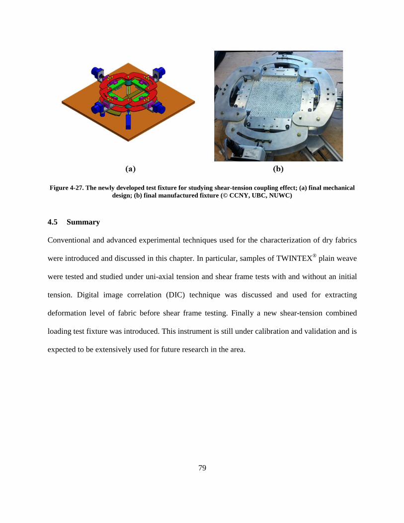
79
Figure 4-27. The newly developed test fixture for studying shear-tension coupling effect; (a) final mechanical
design; (b) final manufactured fixture (© CCNY, UBC, NUWC)
4.5 Summary
Conventional and advanced experimental techniques used for the characterization of dry fabrics
were introduced and discussed in this chapter. In particular, samples of TWINTEX® plain weave
were tested and studied under uni-axial tension and shear frame tests with and without an initial
tension. Digital image correlation (DIC) technique was discussed and used for extracting
deformation level of fabric before shear frame testing. Finally a new shear-tension combined
loading test fixture was introduced. This instrument is still under calibration and validation and is
expected to be extensively used for future research in the area.

80
Chapter 5: Meso-level model development
In this chapter, basics of the meso-level fabric modeling and its application are introduced and
then, using data from Chapter 4, an inverse identification technique is proposed to extract the
material properties of yarns in the TWINTEX material under study. Finally, the fully
characterized meso-level model is validated to ensure correct predictions of the fabric response.
5.1 Introduction
As mentioned earlier the multi-scale nature of woven fabrics makes it literally impossible to
develop a single, complete model that includes all aspects of a fabric from individual fibers to
the final part geometries. Therefore, usually woven fabrics and their forming are studied in
different scales which include: micro, meso and macro levels. Although a final part is in macro-
scale, studying the behavior of woven fabrics in meso-scale is of particular interest. One of the
most important reasons for efforts in simulating fabrics at meso-scale is the fact that if a reliable
meso-level model is available for simulating fabrics deformations, it can be used to run virtual
experiments to estimate macro-level response of the fabric (Boisse et al., 2001; Lee et al., 2009;
Peng & Cao, 2000). Indeed, numerous new loading modes can be studied on a meso-level model
which could bear high cost if run by physical samples.
5.2 Finite element simulation of fabric at meso-level
Every finite element model has different features depending on the given applications and
conditions. Details of the finite element model targeted here for woven fabrics are discussed
under four different categories as follows:
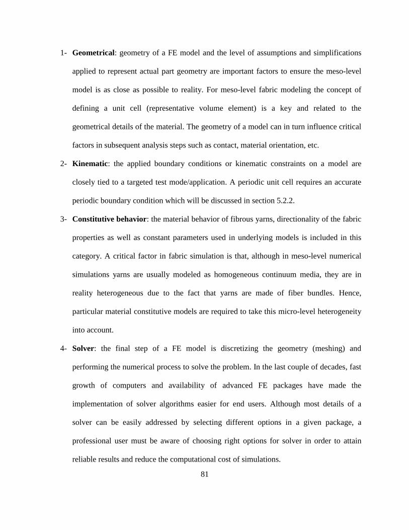
81
1- Geometrical: geometry of a FE model and the level of assumptions and simplifications
applied to represent actual part geometry are important factors to ensure the meso-level
model is as close as possible to reality. For meso-level fabric modeling the concept of
defining a unit cell (representative volume element) is a key and related to the
geometrical details of the material. The geometry of a model can in turn influence critical
factors in subsequent analysis steps such as contact, material orientation, etc.
2- Kinematic: the applied boundary conditions or kinematic constraints on a model are
closely tied to a targeted test mode/application. A periodic unit cell requires an accurate
periodic boundary condition which will be discussed in section 5.2.2.
3- Constitutive behavior: the material behavior of fibrous yarns, directionality of the fabric
properties as well as constant parameters used in underlying models is included in this
category. A critical factor in fabric simulation is that, although in meso-level numerical
simulations yarns are usually modeled as homogeneous continuum media, they are in
reality heterogeneous due to the fact that yarns are made of fiber bundles. Hence,
particular material constitutive models are required to take this micro-level heterogeneity
into account.
4- Solver: the final step of a FE model is discretizing the geometry (meshing) and
performing the numerical process to solve the problem. In the last couple of decades, fast
growth of computers and availability of advanced FE packages have made the
implementation of solver algorithms easier for end users. Although most details of a
solver can be easily addressed by selecting different options in a given package, a
professional user must be aware of choosing right options for solver in order to attain
reliable results and reduce the computational cost of simulations.

82
In the following sections, details of all the above steps for the current research are presented and
discussed.
5.2.1 Geometrical details
5.2.1.1 Unit cell
Considering the meso-level structure of a woven fabric, hundreds of yarns are interlaced to
produce the fabric. Because the simulation of the whole fabric is impractical (if not impossible in
some cases) a unit cell of the fabric is selected for analysis (Badel et al., 2007; Bakhvalov &
Panasenko, 1989; Peng & Cao, 2002). The idea of the unit cell is based on the periodic nature of
fabrics. Basically, it can be said that a unit cell is the smallest element that by repeating in two
directions in a plane, the full geometry of the fabric can be created. Figure 5-1 shows the fabric
geometry and the selected unit cell for the TWINTEX material in this study. It clearly shows that
geometrically repeating this unit can result in the geometry of the whole fabric. Although it has
been proposed by some researchers that using kinematic conditions such as symmetry,
translation, rotation and reflection can help reduce the size of this unit cell in simulations (Li et
al., 2011), it was decided not to use these conditions in here because the overall time of running
each simulation is not considerably high (in order of a couple of minutes).

83
Figure 5-1. Selected unit cell for a balanced plain weave
5.2.1.2 The yarn and yarn path geometry
It is not possible to define a single curve equation that can precisely describe the path or
geometry of all fibers. As is mentioned before, each yarn consists of a bundle of fibers; this in
turn makes it also hard to define a certain boundary or shape for the cross section of a yarn.
Moreover, the fabric interlacing/weaving process induces a complicated curvilinear shape on the
path of yarns. In general, it can be said that due to all uncertainties incorporated into the nature of
yarns and their weaving, the shape and path of a yarn are rarely repeatable. However, in order to
facilitate the analysis using the meso-level modeling there are suggestions for analytically
defining a path and cross sectional shape for the yarns. The simplest way is using circular
sections and straight lines and to define proper contact conditions and avoid penetration at cross
over points; the path can also be changed to be circular (Peirce, 1937). Later on, this definition
was evolved into similar ideas by the introduction of elliptical, lenticular, sine and other
geometrical shapes (Hu, 2004; Mcbride and Chen, 1997). More complex models are being
developed every year in order to capture different yarn paths and geometries; nonetheless, all
those models should satisfy some minimum requirements to be suitable for meshing and FE
simulations (Hivet and Boisse, 2005), among which the penetration between yarns at cross over

84
points is one of the crucial ones. One approach to avoid the difficulty of dealing with fabric
geometrical complexities and programming for design of yarns geometry is using available
software packages that are particularly developed for studying yarns at meso-level.
For example, TexGen® is an open source software package and flexible in defining almost any
type of yarn path and geometry (Sherburn, 2007). Using a periodic spline for defining the yarn
path and lenticular cross section is suggested as default. This type of path and cross section is
selected in the current work as it is proven to be relatively accurate and consistent in 3D
modeling of fabrics (Hivet and Boisse, 2005; Sherburn, 2007). As mentioned in Chapter 4:
generally, an ideal balanced plain weave can be defined by three geometrical constants (Mcbride
& Chen, 1997; Peng & Cao, 2002): the yarn spacing (S), width (w) and yarn thickness/height (h)
(see Table 4-1 for specifications of the fabric used in this research). In the TexGen software,
details of the yarn spline and cross section can be automatically calculated by the software
providing these three parameters as input.
5.2.2 Boundary conditions
As addressed in Section 5.2.1.1, when it comes to modeling fabrics at meso-level, instead of
dealing with a full scale model with an enormous number of yarns, it is preferable to define a
repeatable unit cell. On the other hand, the kinematic conditions on the (in-plane) boundaries of
this unit cell should be defined in a way that the effect of adjacent unit cells and the entire fabric
structure is taken into account. In other words, leaving the surrounding boundaries of the unit
cell free and modeling it as an isolated body will yield completely different results than a unit
cell which is kinematically confined to its neighboring unit cells in a repetitive pattern.

85
The concept of periodic boundary conditions is suggested for this type of situations when
dealing with a substructure whose repeats produces the higher level unit structure (Badel et al.,
2007; Bakhvalov & Panasenko, 1989; Li et al., 2011; Xia et al., 2003). Generally, if the in-plane
boundary/perimeter of the unit cell is shown with , the four sides of the unit cell in the case of a
woven fabric can be divided into four regions as shown in Figure 5-2. Moreover, as it is shown
in the same figure the surfaces of are the same as
in the adjacent cell. So, it can be
intuitively said that the meso-level deformations on one side of the unit cell should conform to
the opposite side.
Figure 5-2. Features of periodically repeating unit cell
In order to formulate this condition, it can be said that generally the deformation/displacement
(as well as some other field variables that are not covered in here such as temperature etc.) in a
unit cell can be decomposed into two components of macroscopic (average) part and periodic
(local) fluctuations (Badel et al., 2007) as follows:

86
( ) ( ) ( ) (5.1)
where ( ) is the displacement vector at a point initially located at and
subscripts m and p refers to the component related to the macroscopic and fluctuating component
of the displacement, respectively (Figure 5-3).
Figure 5-3. Decomposition of deformation into macro-level and periodic deformations
Hence, it can be argued that for each two periodically paired points on the boundaries (Figure 5-
2), we have:
( ) (
) [ ( ) (
)] [ ( ) (
)] (5.2)
Considering the fact that the periodic component of the displacement is the same for both sides
of the unit cell (it can be seen from Figure 5-2 that and
are the same boundaries attached
to two adjacent cells):
( ) (
) (5.3)
Therefore,
( ) (
) ( ) (
) (5.4)

87
Note that this formulation does not explicitly provide an output for the displacement boundaries;
the only variable that can be extracted from this equation is the difference between displacements
in two periodically paired nodes.
One important note to add is that, for points that are located on the “corners” (belong to two
boundaries) the periodic component of their displacements is zero (Badel et al., 2007), or in other
words ( ) and ( ) ( ). Therefore, the expected macro-level boundary conditions
can be imposed on these points, whereas the kinematic condition in Equation 5.4 must be applied
to any other two periodically paired points on the boundary. Considering the four corner points
shown in Figure 5-4, three different types of mechanical deformation modes that were discussed
in Chapter 4 (uni-axial tension, shear, and shear-tension combined) can be imposed on the unit
cell using the following equations:
( ) (
) ( ) (
) (5.5a)
( ) (
) ( ) (
) (5.5b)

88
Figure 5-4. The corner points to apply the boundary conditions (red points); two periodically paired points
along the border line (blue points)
This is the general form of the boundary conditions on four corner points where and are the
axial strains along warp and weft respectively and is the shear angle. For each individual
loading mode of interest, the conditions described in Table 5-1 can be applied to impose the
corresponding loading mode. These boundary conditions were introduced into Abaqus via a
user-defined FORTRAN subroutine UAMP which controls the amplitude of displacement on
each point during the deformation. The FORTRAN code for this subroutine is given in Appendix
A.
Table 5-1. Details of applying boundary conditions using the general formula (Eq. 5.5) for each loading mode
Loading mode Details of boundary condition
Uni-axial tension ; ;
releasing @ and
Shear frame ; ;
Shear frame + tension along yarns ; ;

89
Moreover, the kinematic boundary condition as it was presented in Equation (5.4) can be
incorporated into Abaqus for every other point located on the boundary using a Multi-Point
Constrain (MPC) user-defined subroutine. This subroutine is defined to establish a relation
between degree of freedom (DOF) for each two periodically paired points. In the case of
homogeneous macro-level deformations, it can be said that the macro-level deformation of each
point on the boundary can be found by a liner interpolation between two corner points on that
boundary. For example, Equation 5.4 for the periodically paired points of P and P’ in Figure 5-4
can be written as:
( ) ( ) [ ( ) ( )( )] [ ( ) ( )( )]
(5.6a)
( ) ( ) (5.6b)
This boundary condition is also introduced into Abaqus by MPC subroutine which is given in
Appendix A. Nodes located in the surrounding surfaces of the unit cell need to be properly
paired before sending to MPC subroutines in order to establish proper kinematic constraints
between corresponding nodes. Generally, TexGen is capable of conveniently conducting this
task. For the unit cell used in here, because of changes made in the defaults of the unit cell in
generating its geometry (changing the number of yarns and the box that defines the domain), the
software failed to do so. Therefore, a MATLAB code was generated to identify nodes located on
the periodically paired points and create arrays (node sets in Abaqus) with the right order (i.e.,
paired nodes on each array are given same indices) to establish the correct kinematic constraint

90
using MPC. Figure 5-5 shows the nodes that are identified and paired using the MATLAB file
(paired nodes have the same color).
Figure 5-5. Paired nodes in the meso-level model using a MATLAB code
5.2.3 Material constitutive model for yarns
This aspect of modeling should again be linked to the multi-scale nature of woven fabrics and the
fact that although in their finite element simulations it is often assumed that yarns are
homogeneous continuum media, in reality, they are composed of hundreds of thin and long fibers
(Figure 5-6). In the case of textile structural fabrics, where yarns are made of continuous
filaments, fibers have extremely large length-to-diameter ratios. This suggests that fiber bundles
are not capable of carrying compression loads. Moreover, before consolidation there is no
bonding between fibers and they can easily slide on each other, therefore, the transverse stiffness
and shear modulus for yarns are very small in dry pre-forms. On the other hand, continuous
fibers show a notable stiffness and strength when loaded along fibers direction in tension.
Nonetheless, this is only along fibers and therefore, during simulation accurate procedures must
be planned for tracking this material direction. The transverse stiffness of the dry yarns acts in a

91
very nonlinear manner. At micro-level, the small empty spaces that exist between fibers results
in a very low stiffness under transverse compression for yarns; but for example after the tensile
deformation of fabric proceeds, the distance between the fibers are decreased and there can be
more significant side to side intra-yarn contact forces which means more compressive stiffness
of the yarn cross section in meso-level.
Figure 5-6. Tomography image showing fibers in a sample of woven fabric textile composite laminate
(courtesy of Dr. Shah Mohammadi, UBC Okanagan)
There has been notable effort in the field to take into account the effects mentioned in the
previous paragraph at meso-level fabric simulation models. Gasser et al. (2000) and Boisse et al.
(2001) suggested using zero values (or quasi zero: using very small values for the sake of
numerical convergence) for all the shear stiffness modulus components (G12, G23, G13) and
Poisson’s ratios (ν12, ν23, ν13), and using a nonlinear form of transverse stiffness (E22, E33) as
follows:
| |
(5.7)

92
where E0, n and m are constants to be determined via an inverse identification using results of its
mechanical tests on fabrics such as biaxial tension (Gasser et al., 2000).
The axial stiffness along fibers (which is ideally the same direction as yarn path) has the highest
stiffness values compared to other components of stiffness. Moreover, considering the fact that
due to yarn undulation under axial tension and yarn trellis under shear, the direction of fibers
changes during deformation, an accurate measure for tracking fibers direction and applying
appropriate orientation of the material is highly important during modeling. The important point
is that, although the initial material direction may be correctly assigned inside each yarn, it can
deviate from the yarns direction during the stress updates. In fact, a considerable difference
between the stiffness in the yarn direction and other directions can result in unacceptable errors
even if a small drift happens between the actual orientation of fiber and the direction of stress
updates in the finite element coordinate system. Figure 5-7 illustrates this fact showing the
actual material frame/direction of fiber (the orientation that must be used for the correct material
properties during deformation) and comparing it to another frame that is used by the software
which may result in inaccurate results. The mechanism of controlling material frame/orientation
is one of the biggest challenges in modeling fabrics in meso-level which often requires high level
of modifications to the solver of finite element package (Komeili & Milani, 2010). Handling of
this condition in a commercial FE package such as Abaqus is discussed in the following section.

93
Figure 5-7. The deviation of initial material orientation/frame from the working frame of finite element that
should be considered during stress updates
5.2.4 Hypo-elastic modeling and yarn orientation considerations
The finite element simulations for non-linear behaviors, including non-linear material properties
and large deformations, are usually solved in a step-wise manner. This enhances the convergence
in a non-linear finite element analysis and improves the drifting error (Felippa, 2001). Basically,
the state of stress and deformation along with the kinematic (displacement and strain) and
kinetics (loading and stress) data for each element in each step is used to predict/extrapolate the
next step’s variables. This is done by numerical integration of rate of constitutive equations
(Healy and Dodds, 1992). In an explicit finite element method the sole step of updating field
variables is considered sufficient whereas in an implicit finite element method, another set of
algebraic iterations within each time step is conducted to assure the equilibrium. There are
numerous references that elaborate on details of these two categories of finite element methods
and their applications (Felippa, 2001; Zienkiewicz and Taylor, 2000). For fabric modeling, the
stress update in each step (in both FE methods) is done according to the following hypo-elastic
formula (Badel et al., 2008; Boisse, 2010):
(5.8a)
( ) (5.8b)

94
where , and are the objective derivative of the stress tensor, constitutive tensor and the
strain rate tensor in the current material coordinate system (which is determined by the default
objective derivative used by the software), respectively. is in turn the symmetric part of the
spatial rate of deformation tensor ( ), which is calculated from the rate (shown by dot on the
symbol) and inverse of deformation gradient tensor ( ) as shown in Equation (5.8b) (Mase and
Mase, 1999). The number of bars underneath the symbol shows the order of the corresponding
tensor. The challenging part of this formulation is dealing with the definition of objective
derivative. The goal of objective derivative is to avoid the rigid body rotations that can affect the
stress state. In other words it is to assure that the derivative of stress in the original (initial) frame
of material is the same as the derivative of stress in the frame that is rotated due to rigid body
motion in large deformations. The objective stress derivative update in a hypo-elastic material
model is done by the following formula (Badel et al., 2009; Healy and Dodds, 1992; Peric and
Owen, 1992):
(
( )) (5.9)
where,
(5.10)
is the Cauchy stress (Mase and Mase, 1999) and is a rotation tensor whose definition
depends on the selected stress objective derivative (dot shows the rate with pseudo-time). For a
derivative to be objective, must be associated with the rigid body rotation (Badel et al., 2009).
In a numerical FE package the estimation of objective stress is used to update the stress at

95
current step (n) and predict stress values in the next time-step (n+1). More details on this
integration are discussed later in this chapter and can be found with more elaborations in
numerous references (Badel et al., 2009; Healy and Dodds, 1992; Ogden, 1997). There are
different objective derivatives for stress, however, the two most common options widely used in
available finite element packages are Jaumann (1911) and Green-Naghdi (Green and Naghdi,
1965). In the former, the spin rate tensor ( ) is used for in Equation 5.9 (Healy and Dodds,
1992):
( ) (5.11)
Alternatively, the Green-Naghdi approach assigns (Badel et al., 2009) where is
the polar rotation tensor which can be derived from the deformation gradient tensor using the
following relationship (Mase and Mase, 1999):
(5.12)
in which and are the right and left stretch tensors, respectively. Although both of these stress
derivatives are objective and remove the effect from rigid body rotation in defining the
frame/directionality of the stiffness tensor ( in Equation 5.8), there might be a deviation
between the ensuing transformation tensors between them (e.g., in general). Therefore, a
proper form of stiffness tensor must be used against each method, otherwise using the same set
of constants along with each of the objective derivatives can results in different outcomes (Peric
and Owen, 1992). For the case of dry woven fabrics, according to the discussion mentioned in
Section 5.2.3, it is preferred to have an objective derivative whose transformation tensors are

96
based on the direction of fibers (Badel et al., 2007). Indeed it has been proven that the only
objective derivative which can be used for modeling dry fabric in finite element is the one whose
transformation is based on tracking the direction of fibers (Badel et al., 2009; Badel et al., 2008).
However, the objective stress derivative is usually an internal (built-in) part of a numerical
package and can hardly be changed. For example, Abaqus uses Green-Naghdi objective stress
derivative for its explicit solver and Jaumann for its implicit (also called standard) solver in 3D
continuum elements (SIMULIA, 2010). Nonetheless, a customized material behavior can be
defined via a user-defined FORTRAN subroutine (UMAT for implicit solver and VUMAT for
explicit solver). Basically, the input data for the user-defined material subroutine here are the
deformation variables (e.g., strain, strain increment, deformation gradients), stress and state
variables from the previous step, and other information that might be used for some particular
cases such as the step time and energy. The ensuing output from this subroutine is the new state
of stress. Thus, the input from a previous step can be effectively used along with the deformation
data to calculate customized stress update algorithms for the next step. The practice of defining
customized material behavior for Abaqus has been used extensively in modeling of dry fabrics at
meso-level (Badel et al., 2008; Komeili & Milani, 2011; Komeili & Milani, 2010; Lin et al.,
2009).
In general, it can be said that there is only one transformation tensor/matrix which can relate the
working frame of the software with unit base vectors where , to the frame attached
to the fabric with unit base vectors . The former can be the frame that is rotating with the
Jaumann or Green-Naghdi transformation and the latter is defined in a way that the first local
unit vector ( ) is always in the direction of fibers (for details see Appendix B: Transformation

97
matrix of fibers). In summary, the transformation matrix can be defined as following between
these two coordinate systems as follows.
[ ] (5.13)
is a 6 by 1 vector which can be replaced by stress or
strains vectors as well as their increments, and [ ] is the corresponding 6 by 6 transformation
matrix. It is to note that the vector representation of the variables above is to make it easier for
implementing in Abaqus user-defined subroutines. More details on the transformation matrix
([ ]) are provided in Appendix B along with the user-defined subroutine in Appendix A that has
been used during the subsequent simulations. Having this transformation matrix, there are two
methods suggested for updating the stress tensor (Badel et al., 2009; Badel, et al., 2008) as
follows.
5.2.4.1 Transforming Stress and Strain matrices (TSS)
This method can be summarized in three steps: (1) transforming the current stress, strain, and
strain increment vectors from the frame of software ( ) to the frame of fibers ( ), (2) updating
stress values using a material stiffness matrix defined with respect to the current fiber direction,
and (3) transforming it back from the frame of fibers to the frame of software for reporting the
final output. For the first step:
[ ] (5.14a)
[ ] (5.14b)

98
The superscript ‘n’ on the stress and strain increment refers to the current time step of the
numerical simulation and [ ] is the inverse of the transformation matrix [ ], such that
[ ] [ ] [ ] where [ ] is a 6 by 6 identity matrix. For the second step:
[ ] { }
(5.15)
Note that the above formula is a simplified version of integration formula discussed in Section
5.2.4. What is required at the output for the software is the stress at the next time step in the
working frame of software ( ). The last transformation, for the third step, is done using
the following formula and subsequently the updated stress is reported in the software output.
[ ] (5.16)
5.2.4.2 Transforming Stiffness Matrix (TSM)
Another alternative to the above mentioned approach (TSS) is transforming the stiffness matrix
from the frame of fabric to the frame of software and updating the new step directly in the frame
of the structure using the transformed stiffness matrix. In other words:
[ ] [ ][ ] [ ] (5.17)
And then,
[ ] { }
(5.18)
5.2.5 Comparing TSS and TSM in practice
Considering the fact that there are two options for stress updates using a particular user-defined
material behavior (TSS or TSM) and two options for the numerical solver/integrator (implicit or
explicit), at least four different approaches are available for the meso-level fabric simulations in

99
practice. In order to select the best combination for this research, a comparative study was
conducted by Komeili & Milani (2011) on the selection of the above four different candidates as
well as some other details of fabric finite element simulation (e.g., shear stiffness and hourglass
stiffness effects). In their study, a simple case of a cubical shape was subjected to displacement
boundary conditions as shown in Figure 5-8.
Figure 5-8. The simple geometry used for comparing different stress update methods and its loading
condition (dimensions of cube are 20×20×20 mm)
It was assumed that the cube is made of fibers located along the z-direction. Accordingly, the
stiffness in z-direction is taken to be much higher (50 GPa) compared to the stiffness in the
lateral direction and for the shear (5 MPa). Regarding the given imposed boundary
displacements, a logarithmic strain value of 0.03845 was calculated analytically along the fiber
direction which results in a stress value of , in a frame that follows the
orientation of fibers. A comparison between reported stress values between the user-defined
simulation codes in Abaqus using TSS, TSM methods as well as the default objective stress
The main axial
stiffness
direction
uy = 4 (mm)
ux = 4 (mm)
x
yz

100
derivative option by the software (Jaumann for implicit/standard solver and Green-Naghdi fot
explicit solver) is presented in Table 5-2.
Table 5-2: Obtained axial stresses (σz) using different combinations of integrator/material models and their
error percentages compared to the analytical solution of the problem shown in Fig. 5-8
Method Explicit Implicit
σzz (GPa) Error σzz (GPa) Error
Default 0.994 48.3% 1.013 47.3%
TSM 1.983 3.1% 1.961 2.0%
TSS 1.983 3.1% 1.961 2.0%
Moreover, in order to check the computational cost of each option, a more detailed analysis on a
unit cell model similar to the one in Figure 5-1 was conducted under three loading conditions:
uni-axial tension, biaxial tension and trellising shear. For uni-axial and biaxial tensions a strain
value of ε=19.5×10⁻³
was selected for simulation and for shear trellising a shear angle of
was applied.
It was reported that the convergence range (the percentage of analysis completion before
divergence; in cases that divergence happened) is different for each integrator type under
different loading conditions. However, in general implicit integrator showed superiority to the
explicit integrator. Charts in Figure 5-9 roughly show the computational efficiency of each
method by illustrating the ratio of run time to the convergence range (the percentage of
completion of the analysis before it stops due to numerical divergence).

101
Figure 5-9: The normalized run-time for each simulation. Note that the simulation could not converge for
shear in the explicit integrator
Therefore, the implicit integrator was selected for the rest of analyses in this research. It should
also be mentioned that in comparison to the explicit integrator, the implicit integrator uses the
stiffness matrix in each time step for internal iterations. Therefore, the user-defined subroutine
for implicit integrator (UMAT) needs to include the stiffness matrix as well as the stress updated
at the end of each step. On the other hand, the only required output for the subroutine in the
explicit solver is the stress update. Details of implementing these techniques are provided by
(Komeili & Milani, 2010).
5.3 Inverse identification
The next step of modeling was to quantify the stiffness matrix of yarn in the fiber coordinate
([ ] ) in Equations (5.15) and (5.17). Measurement of material properties such as stiffness and
0
2
4
6
8
10
12
14
16
TSM, Implicit TSS, Implicit TSM, Explicit TSS, Explicit
No
rmli
zed
ru
n t
ime
Selected method (stress update, integrator)
uni-axial
bi-axial
shear

102
strength in homogeneous conventional materials such as most metals can be done via testing a
sample in displacement or force controlled conditions. However, for geometrically multi-scale
materials such as woven fabrics this cannot be done as conveniently. The measurement of fabric
response in macro-level such as axial stiffness (Buet-Gautier and Boisse, 2001) and shear (Cao et
al., 2008) can be performed, e.g., from uniaxial tension and shear frame tests. However, the
properties of yarns are harder to measure directly, especially considering the fact that running
tests on a straight yarn as a single identity may be meaningless. A single yarn before weaving
cannot reflect the properties of a yarn that is woven inside a fabric, because of tension and
damages that are induced during the weaving process (Chou and Ko, 1989).
The second difficulty in measuring the mechanical properties of yarns in a fabric is the fact that
some of these properties are related to the interactions between yarns as a whole system. For
example, the interaction of fibers at cross over points, which is due to contact and interlacing of
yarns, is the main factor for determining the non-linear form of the transverse stiffness. It has
been shown that a proper use of transverse stiffness (crushing formula) can assist in more
accurately modeling fiber interactions and local deformations at cross over points (Badel et al.,
2008). This brings the need for a very accurate inverse identification strategy for woven fabric
materials.
There are numerous investigations on model identification of composites that have used inverse
identification in macro (Milani and Nemes, 2004; Milani, 2005) and meso-levels (Gasser et al.,
2000; Komeili & Milani, 2012). The principle behind an inverse identification is described
below.

103
Assume the response of a material system, regardless of the underlying deformation mechanism
(i.e., considering the system as a black box), to a set of controlled inputs is given by the
following function:
( ) (5.19)
is the vector of input variables, is the response of the system, and ( ) is
the unknown function to be identified. In general, the analytical form of the latter function for
complex multi-scale materials is not available and it is impossible (or extremely complicated) to
extract. However, observations on the system output to different inputs are normally possible
through running experiments with a set of known controlled inputs ( ). For a given number (n)
of experimental inputs which results in the same number of output variables, the following set of
data points can be generated:
( ) (5.20)
Because the general form of the ( ) function is not known, it is widely accepted to use an
approximating function with a set of unknown coefficients (Wu and Hamada, 2009).
Nonetheless, it must be selected with a trend similar to the observations made from experiments.
The predicting function can be represented as:
( ) (5.21)
where is the predicted output from the given set of inputs and the set of constants
. Because the approximation function is deterministic and it is not mimicking the
exact observations in practice, there is a residual, ,value associated as follows:
( ) ( ) ( ) (5.22)

104
In practice it might not be possible to completely eliminate the error, however by choosing a
proper approximating function and minimizing the residuals at different observed points and
finding the optimum values for , it can be reduced to an acceptable level.
Considering the fact that there are known data points ( ) through experiments, the above
formula can be expressed as:
( ) ( ) ( ) (5.23)
Accordingly, ( ) is a vector of ‘n’ discrete values that are functions of . Figure 5-10
illustrates a schematic of data points and an approximation function as well as the resulting
residual values.
Figure 5-10. The discrete values of real response from experiment ( ) are compared to the response
predicted from model ( ) to obtain the residual/error ( ).
For minimization of all error values, a norm of ( ) vector can be used. Among norms
available for evaluating a vector (Lancaster and Tismenetsky, 1985), the Euclidian norm is
commonly used for curve fitting and inverse identification purposes in numerical simulations

105
(Felippa, 2001; Gasser et al., 2000; Milani, 2005). The Euclidian norm for the vector ( ) is
defined as (Lancaster and Tismenetsky, 1985):
( ) ‖ ( ) ‖ √∑| ( )|
(5.24)
Minimizing the ( ) for the values (which are constants in the model ( )) is the last step to
identify a function for the observed material behavior through the standard least squares method:
( ) (5.25)
Therefore, choosing a proper optimization scheme is also necessary in order to solve equation
(5.25) which will be discussed in the following section.
5.4 Multi-objective optimization
The statements made above for the inverse identification for one experimental mode (e.g., uni-
axial tension) can be expanded to the inverse identification on a system using different test
modes/output variables (i.e., different categories of values). Assuming two experimental
modes running on a material system (uni-axial tension and shear test in this case), the output of
each test is a separate variable such as:
( )
( ) (5.26)
where superscript refers to the test mode. Similarly, each residual can be written as:
( ) ( ) ( ) (5.27)

106
which results in ( ) for each experimental mode. Hence, the minimization formula in
Equation (5.25) can be expressed as:
( ) (5.28)
where,
( ) ∑ ( )
(5.29)
are the scale factors used when the output variables have values of different order of
magnitudes, and are the weighting factors which is used to adjust the importance of selected
modes. Indeed, the biggest difficulty in this multi-objective minimization is the fact that there is
no unique answer for choosing these weights. Whereas in a single objective optimization it can
be argued that there is at least one vector which is absolute extremum, such an argument can
rarely be made in a multi-objective problem. As a result, the term Pareto-optimal (Pareto front)
is often used in dealing with multi-objective problems. A solution is Pareto-optimal if it is not
dominated by no other feasible solution (Lampinen, 2000). The Pareto-optimal solution points in
a Pareto front are schematically depicted in Figure 5-11a. Assuming that each objective function
can be evaluated for every input variable in optimization (in this case ), the mapping from to
the (only 2 objectives are selected for illustration purpose) will result in a set of feasible
solutions in the blue region of Figure 5.11a. Then, it can be argued that every point on the Pareto
front (red curve) is superior to other points inside the blue region. In other words, points inside
the blue region are dominated by points on Pareto front. For example, point P1 is dominated by
P2, and P3, because having the same value for , P3 has a lower ; and similarly having the
same value of , P2 has a lower . Whereas, for instance, P3 is not fully dominated by any

107
other point because there is no other feasible point which has the same or lower values of both
and than those of P3. In the case of numerical simulations, there are often a limited number of
points that can be generated, so the Pareto front would be estimated in a discrete space similar to
Figure 5-11b.
Figure 5-11. The Pareto front (a) with full mapping from space of variables to objectives; P1 is dominated by
several points including P2 and P3; (b) Pareto front estimated with discrete values and limited number of data
points
It can be said that all the points that are Pareto-optimal are possible solutions to the multi-
objective optimization problem. In order to choose only one solution with one set of , the
multi-objective problem may be reduced to a single objective problem via Equation (5.29). Here
it is the decision of the designer/data analyzer to choose proper values of weighting factors based
on the priorities of the given application or even the confidence in outcomes of the
simulations/experiments (Milani, 2005).
5.5 Implementation of multi-objective optimization for current case study
The goal here is to establish a material constitutive model which is suitable for studying the
TWINTEX plain woven fabric under general in-plane loadings including axial tension and shear.

108
Although, results of axial tension tests on individual yarns were used by other researchers to set
the axial stiffness of yarns (Charmetant et al., 2011; Chou & Ko, 1989), inverse identification via
biaxial tension tests has also been practiced in the past to arrive at formulations of transverse
stiffness (Badel et al., 2007; Badel et al., 2008; Gasser et al., 2000). Komeili & Milani (2012) for
the first time suggested an inverse method using multi-objective optimization for identifying
axial stiffness as well as transverse stiffness constants for a sample of E-glass fabric. Similar
procedures are pursued here. The general form of the total objective function is expressed as:
( ) ∑ ( )
( ) ( ) (5.30)
denotes the objective function and the total error in the uni-axial tension mode ( ), and
indicates the shear frame test ( ) with an initial tension, as discussed in Section 4.4.5.3.
The reason that the pre-tensioned shear frame test was selected here is simply because it can be a
better indication of simulations to be ran on the effect of combined (shear + tension) loading.
The sets of input variables defined are for shear frame test, and for
uni-axial tension. The optimization variables ( ) are the material constants in the stiffness
matrix of the yarns. The stiffness matrix of yarns can be put in a proper form for this
optimization purpose as follows:
[ ]
[
]
(5.31)
where,

109
{
| |(| | ) (| | )
| |(| | ) (| | )
( | |)
(5.32)
In this case the variables of optimization are . And there is another
set of user-defined constants shown as in Equation (5.32) which are merely used to assure
numerical stability for the cases where the stiffness should be set at very low quasi-zero values
(Gasser et al., 2000). In this study, , and are used, where
. The formulation of the transverse stiffness in Equation (5.32) is selected close to
the suggested form by Gasser et al. (2000) with proper modifications to take into account the
lower stiffness when there is tension in lateral direction. Basically, the dry yarns cannot bear any
stiffness when they are pulled in the lateral direction because there is no bonding between fibers,
whereas they are crushed against each other in lateral compression.
Results of experiments from uni-axial tension (Figure 4-9) and average response from results of
the shear test with pretension (Figure 4-22) were used as the observed data points ( ( )).
Then simulations were run in Abaqus using the material constitutive model discussed above and
optimization was run on variables. The whole process of running Abaqus simulations,
comparing results to the experimental data, and running the optimization was automated in
Isight®
software (Komeili & Milani, 2012; SIMULIA, 2011). A schematic of the Isight flow-
model used is shown in Figure 5-12. The optimization process is accomplished in the bigger loop

110
shown in Figure 5-12. Each time that the loop is run, one value is extracted for the total objective
function. Each one of the small loops calculates the value of objective function for uni-axial
tension or shear following five steps:
1- Abaqus runs with the set of that are passed to from a given iteration of the optimization
algorithm.
2- Python script reads the reaction forces at four nodal points at the corners of the unit cell
(Figure 5-4) which impose the corresponding loading boundary condition, and saves
results in an ASCII file.
3- Data are read from the ASCII file and saved in new internal variables defined in Isight.
4- Latter variables having values from ASCII files are copied in an Excel file which has
functions for calculating shear force and/or axial tension force in the unit cell from nodal
forces on four corners (more details of this calculation is discussed in Section 5.5.1).
Then the total response force of the unit cell (axial or shear) is read from the Excel file.
Moreover, the data from experimental measurements are stored in the Excel file which
are read by Isight.
5- The normalized force responses (Komeili & Milani, 2013; Peng et al., 2004) at data
points from both simulation and experiment are compared to calculate the Euclidian norm
of residual vectors ( ( ) ), which is then used as objective function for that particular
loading mode.

111
Figure 5-12. The Isight flow-model used for running optimization process for inverse identification of yarns
material properties (details of each step is discussed above)
5.5.1 Extracting global force response from nodal reaction forces
As mentioned before, the predefined displacements at four corners of the unit cell are the way of
imposing the corresponding loading condition, in each deformation mode. Considering the unit
cell of the fabric as a rectangle before deformation, the macro-level displacement field is a
parallelogram as shown in Figure 5-13. Force equilibrium equations must be used to extract the
magnitudes of tension force in yarns along warp and weft (
and
, respectively) and
shear forces ( and ) from these nodal points. Forces at four nodal points on corners of
unit cell are equivalent to the axial tension and shear forces (
,
and ) on the
selected edges as shown in Figure 5-13. Note that, these forces (
,
and ) are
the reaction forces that are exerted from fabric on nodal points so the direction of forces shown
are opposite of what is seen on the unit cell side. Also similar argument about reaction forces on
the corners of unit cell can be made on the other edges; nonetheless the final results will be the

112
same keeping in mind the overall periodicity of the unit cell. Considering that
,
,
and are alternatives/equivalents to ,
, ,
, and
on each edge, the
following equilibrium equations must hold:
(
) (
) (5.33a)
(
) (
) (5.33b)
(
) (
) (5.33c)
(
) (
) (5.33d)
Equations (5.33a) and (5.33b) are for the edge on the left side, while (5.33c) and (5.33d) are for
the bottom edge. Because each pair of the latter equations refers to the equilibrium on different
edges, they must be solved separately. Accordingly, solving the system of equations in (5.33a)
and (5.33b) for
and :
(
) ( ) (
) (
)
( ) (5.34a)
(
) (
) (
) (
)
( ) (5.34b)
Similarly solving (5.33c) and (5.33d) for
and :
(
) (
) (
) (
)
( ) (5.34c)

113
(
) (
) (
) (
)
( ) (5.34d)
Note that theoretically for a fully balanced fabric, (and the corresponding shear stress
component in the non-orthogonal coordinate system) is expected to be equal to (and its
respective shear stress); for more details see (Peng & Cao, 2003). Our numerical results on the
balanced plain weave also showed that these two force components are literally the same (the
difference was in the order of < 0.1% and was presumed to be due to round-off errors during
numerical calculations). In addition, the warp and weft forces in an equi-biaxial ( )
tension (with or without shear) are checked to be equal in their numerical values.
Figure 5-13. Reaction forces on the nodal point for finding tension and shear forces on the fabric
After running each simulation and imposing boundary conditions on the nodes, the above
formulation was used to extract shear forces and normalize them in order to be compared with
the results of experiments. Normalization of tension forces was done by finding the force per unit

114
length. Whereas for shear force normalization, an energy-based method (Komeili & Milani,
2013; Peng et al., 2004) was employed as in Eq. (4.5).
5.6 Results of inverse identification
The inverse identification was ran using the MIGA (Multi Island Genetic Algorithm) method in
Isight (SIMULIA, 2011). Running the multi-objective form of optimization was necessary since
the characterized model is to be used under general in-plane loading conditions (Komeili &
Milani, 2012). Moreover, it was realized during the optimization that there is a high possibility of
convergence to local minima and the process can be highly sensitive to initial guess of .
Therefore, a genetic algorithm optimization was used to reduce the risk of converging to local
minima. First, the analysis was run for single-objective optimization on each mode. Then, the
value of optimum objective functions were found at the end of single-objective optimizations for
tension and shear ( , ) and the value of scale factors was
accordingly set to the reciprocal of the above objective functions ( ( ) ,
( ) ). As mentioned before, all the points located on Pareto front can be claimed as
possible solution; however it is up to the analyzer to choose the proper point between them by
deciding on the weighting factors in Eq. (5.25). A few numbers of initial iterations were
conducted and the comparison between the response from simulations and experiments was
qualitatively made in order to attain an agreeable response for both tension and shear modes.
Eventually the weighting factors of and were selected and the final results
are shown in Figure 5-14. Result of this multi-objective inverse identification for estimating the
material constants of the yarns constitutive model is summarized in Table 5-3.

115
Table 5-3. Result of inverse identification
Parameter
Value obtained from
inverse identification 9.39 (GPa) 70.22 (GPa) 72.66 (GPa) 44.36
Figure 5-14. The force response of model characterized via inverse identification and compared to the
experimental results; (a) uni-axial tension; (b) shear frame with pre-tension
Remark: The reason for having a high difference between weighting factors of the tension and
shear modes can be further explained due to dominant sensitivity of the total objective function
on the tension mode compared to the shear mode. Namely, without any weighting factor, the
overall objective function, , (Equation 5.30) was seen to be highly affected by the uniaxial

116
objective function, , rather than the shear objective function, . In that case, although the
acquired parameters would still belong to Pareto optimum set, the objective function of the
uniaxial tension mode was overly minimized, to the extent that the objective function of the
shear mode was not minimized enough to accurately capture the picture frame experimental
points. Thus, higher weighting factors needed to be tried for the shear objective function in order
to balance out the dominant effect of the uniaxial objective function on the overall prediction of
the model in both deformation modes. Figure 5-15 shows some of the obtained optimum points
during these weighting trials. The red points are on the Pareto front and the blue point is the
selected final optimum point. From the axis values in Figure 5-15, it is noticed that the Pareto
front in this specific multi-objective identification problem has been much steeper on the
direction of uni-axial tension objective function.
Figure 5-15. Some of data points generated during the optimization process in inverse identification; the red
points are those on the Pareto front where the blue point shows the optimum point selected using the above
mentioned weighting and scale functions

117
It should also be mentioned that in this work only a nominal experimental response was selected
and the inverse identification was conducted based on the assumption that there is a uniform
uncertainty in the results at every given data point. However, in order to increase the accuracy
the signal-to-noise analysis could be incorporated into the analysis (Milani, 2005). Moreover, the
sensitivity of the outcome as a result of choosing different weighting factors could be conducted
to asses the robustness of the results. Nonetheless, this is beyond the objectives of the current
research and the study can be proposed as a new topic.
5.7 Validation
In order to verify identified yarn material properties and the whole FE meso-level model in
general, the shear response of the fabric in the shear frame test with no pre-tension (Figure 4-20)
was compared to the results from finalized simulation using constants in Table 5-3. Figure 5-16
illustrates this comparison. The simulation results are in a fairly acceptable range of the
experiment data, considering the variations and uncertainties (such as misalignment and
wrinkling) that may happen in shear frame testing without pre-tensioning the specimen (Cao et
al., 2008; Milani, 2005).

118
Figure 5-16. Validating the response of the model using the shear frame experimental results
5.8 Summary
A meso-level FE model of the plain weave TWINTEX® material including its unit cell,
kinematic conditions, periodic boundary conditions and the yarn material constitutive model
were explained in details. A multi-objective inverse identification process along with the
incorporated optimization process was discussed for this fabric and used in conjunction with uni-
axial extension and shear frame experiments from the previous chapter.

119
Chapter 6: Macro-level model development and its applications
Following the thesis flow-diagram of Figure 1-7, using the meso-level unit cell model of the
woven fabric which was characterized in Chapter 5, a set of new virtual experiments were ran in
this chapter to extract the full response of the TWINTEX fabric to the in-plane combined loads
(tension + shear). Then, polynomial functions are fitted to the experimental response surface to
obtain a general stress response formulation. Finally, the stress response is used in studying
practical applications at macro-level including the deformation of woven fabric inflatable beams
under torsion and the punch forming of dry fabrics.
6.1 Effect of combined loading
The general in-plane response of the plain TWINTEX®
fabric was fully characterized in this
section via running virtual experiments on the meso-model developed in Chapter 5. The selected
ranges of deformations for general model are 0 to 0.01, 0 to 0.01, and 0 to 32°.
Each strain or shear angle value was divided into 10 equally spaced subintervals and all possible
combinations of strain and shear angles were ran. A total number of 103 runs were performed to
extract the full response of the fabric under general (tension + shear) in-plane loading.
Because the final goal was the homogenization of the meso-level fabric material properties for an
equivalent medium at macro-level, the nominal in-plane stress values for a shell medium with
the same thickness and width as the unit cell needed to be evaluated. In order to calculate a
nominal (average) stress value for each unit cell, the axial and shear forces that were obtained
after the analysis were divided by the nominal cross sectional area of the cell (i.e., area of the
side surfaces, in Figure 4-1). Figure 6-1 shows the nominal stress along warp/weft
direction ( ) at different combinations of axial strains as well as shear deformation. Similarly,

120
Figure 6-2 shows the shear stress response of the fabric unit cell to different combinations of
axial strain and shear deformation. As it can be concluded from surfaces in Figures 6-1 and 6-2,
the axial stress response is only affected by axial strains along warp and weft ( , rather than
), whereas the shear response is dependent on axial responses as well as the shear angle. This
also verifies the previous numerical (Komeili & Milani, 2011; W. Lee et al., 2009) and
experimental observations (Buet-Gautier & Boisse, 2001; Cavallaro et al., 2004; Launay et al.,
2008) on the effect of fiber tension on fabric shear rigidity.

121
Figure 6-1. The axial stress response of the unit cell to different combinations of axial strain and shear levels

122
Figure 6-2. The shear stress response of the unit cell to different combinations of axial strain and shear levels

123
It should be noted that the reported stress values in Figures 6-1 and 6-2 are values calculated
after deformation where the two axial strains and shear angle start at zero and proceed to the
assigned maximum values simultaneously. Nonetheless, it can be shown that the sequences of
applying axial strains and shear deformation can change the fabric response (Komeili & Milani,
2011). For example, Figure 6-3 compares the axial and shear responses of the unit cell for
after it is pre-tensioned with , and vice versa, as well as to the response
if the shear and axial tension are applied linearly from zero to the final values simultaneously.
The time in the horizontal axis represents the progress of the total loading in the FE code
(pseudo-time). For the simultaneous loading case, the strains and shear angle increase with a
linear ramp from the beginning to the end, whereas for the sequential case the axial/shear strain
is applied in a time window of 0-0.5 and then fixing the axial/shear strain in yarns, the
shear/axial deformation is applied in a 0.5-1.0 time interval. As it can be seen, the maximum
axial responses are almost the same (despite different history), whereas the shear responses can
be up to ~40% different. However, to avoid too much complexity, at this stage it is assumed that
the responses illustrated in Figures 6-1 and 6-2 (i.e., for when tensile and shear loads are applied
simultaneously) can be a fair representative of deformation in actual fabric forming.

124
Figure 6-3. Comparing the response of the fabric to different sequences of loading for the same level of
deformation; (a) the axial response along yarns (b) shear response
6.2 Extraction of response surface functions for the combined loading
In order to incorporate the material general response shown in Figures 6-1 and 6-2 within an
analytical calculation of deformation or a finite element package for forming simulations, the
response must be formulated into a function with strains and shear angle as input and stress
values as output. Afterward, this function can be used in calculation or included in a finite
0
0.02
0.04
0.06
0.08
0.1
0.12
0.14
0 0.2 0.4 0.6 0.8 1
No
rma
lzie
d r
eact
ion
fo
rce
(N/m
m)
Simulation time
Trellising shear
Simultanouse
Sequential (Axial followed by shear)
Sequential (Shear followed by axial)
0
1
2
3
4
5
6
7
8
9
10
0 0.2 0.4 0.6 0.8 1
No
rma
lzie
d r
eact
ion
fo
rce
(N/m
m)
Simulation time
Axial tension
Simultanouse
Sequential (Axial followed by shear)
Sequential (Shear followed by axial)
(a)
(b)

125
element model via the “fabric” material behavior in Abaqus and defining a customized user
subroutine (VFABRIC).
There are numerous candidate functions for representing the stress responses shown in Figures 6-
1 and 6-2. The literature in the composites field proves that polynomials can be simple but
reliable candidates for this purpose (Boisse et al., 2011; Milani, 2005).
Because the given fabric is assumed to be balanced, the material responses for warp and weft
yarns are deemed the same. Moreover, because of the same reason, instead of using and in
the shear response functions separately, the summation ( ) and difference between them
( ) are used as variables in the corresponding polynomial. Eventually, after trying
different forms the following functions were selected as the response surfaces for axial tension
stress and shear stress. The comparison between the surfaces generated directly from virtual test
data points and the fitted responses are shown in Figures 6-4 and 6-5, respectively. Different
surface layers in these figures refer to different levels of shear angles in Figure 6-4 and different
axial strains in Figure 6-5. The dependency of axial strain on shear angle is neglected as was
shown in Figure 6-1 to be small. This small dependency has also been verified experimentally in
the past (Buet-Gautier and Boisse, 2001). The fitted stress responses are:
(6.1)
( ) (6.2)
( ) [ ( ) ( ) ( )
( )
( )] ( )
where is the shear angle in degree.

126
Figure 6-4. The axial stress response of the unit cell and the fitted function; different surfaces are
representing different levels of γ
Figure 6-5. The shear stress response of the unit cell and the fitted function; different surfaces are
representing different levels of ε1

127
6.3 Application 1: the behavior of inflatable structures
As mentioned in the introduction in Chapter 1, woven fabrics are often used in inflatable
structures for increasing structural strength where the main pressure load is carried by the fabric
under tension. Studying this application and comparing the new (shear-tension coupled) model to
the old (uncoupled) model can provide a valuable insight.
An inflatable beam similar to the study conducted by (Cavallaro et al., 2003) was selected.
Preliminary studies on the bending response of the structure showed that bending is not affected
by the coupling feature. This was a result of the fact that bending is more affected by fibers
tension, which is a function of internal pressure. Indeed, as it is known from the long beams
theory, shear is not an influential factor (Beer et al., 2009). Therefore, the second study was
focused on the torsional response of the composite beam. The geometry of the beam as a circular
shaft, as shown in Figure 6-6, was selected with a length of and the radius of
. Assuming an internal pressure of P inside the beam and considering its geometry to
be close to a cylinder, there were two components of stresses along the circumference and axial
direction of cylinder to extract. Without losing generality, assuming that initially the warp is in
circumferential (hoop) direction and weft is in axial direction before loading (Beer et al., 2009),
we have:
(6.3)
(6.4)
where warp and weft are shown by subscripts 1 and 2, respectively. Assuming a displacement
controlled loading with the twist angle of , which leads to a shear angle of , after the
torsional loading and change in the direction of fibers similar derivations can be used for the

128
equilibrium of forces in axial and circumferential directions (Figure 6-6). Using the force
equilibrium on a differentially small ring and its cross section, the updated values of stresses
under large deformation are calculated from:
(6.5)
( )
( )
( ) (6.6)
Figure 6-6. The geometry of an inflatable beam/shaft under torsion
Having the twist, the torsional reaction moment at the loading end can be calculated as:
[ ( )] (6.7)

129
Using Equations (6.1) to (6.3), a MATLAB® script was used to run different combinations of the
twist angles and internal pressure inside the inflatable beam to find torsional reaction moment.
Note that the stress response formulation in Eqs. (6.1) to (6.3) was given for stress as a function
of strains, hence in order to find the induced strains due to internal pressure and loading
condition in the given application, a root finding algorithm from MATLAB’s internal function
library (fsolve) was used. The results and comparison between the two coupled and uncoupled
models are illustrated in Figure 6-7. As it can be seen the difference in predicted load value due
to the coupling effect is ~5%.
Figure 6-7. (a) The difference in the torsional response of the inflatable beam to different internal pressures
and twist angles; (b) the percentage difference between predicted torsional moment between two models with
and without shear-tension coupling
6.4 Application 2: simulation of fabric forming
The formulas in Equation (6.1) and (6.2) were implemented in a VFABRIC subroutine shown in
Appendix C. It should be noted that the derivative of the stress response formulas (6.1) and (6.2)

130
could also be used to form the stiffness response. Figure 6-8 shows an example of the shear
stiffness derived from derivative of Equation (6.2) in two different levels of shear angle.
However, to keep the formulation in the FE code simple, the stress response can be used directly
without losing details.
Moreover, because dry fabrics are not able to take compression, an algorithm was defined in the
subroutine to check for this condition and in case of compression in the fabric it brings the axial
stiffness down to a small value (5 MPa; zero must be avoided for numerical convergence).
Figure 6-8. Shear stiffness of the fabric as a function of strain along yarns and shear angle, extracted from
stress response formulas
There are still some debates on whether or not using membrane elements (no bending stiffness)
or shell elements can result in the same outcome in forming simulations of fabrics. There are
evidences which argue that for some forming simulations the results are quite the same (Long,
2006) and others which emphasize the importance of including bending stiffness (Boisse et al.,

131
2011) in fabric response. Nonetheless, in general, shell elements are expected to yield more
accurate responses, but are computationally more expensive. Here, four node shell elements in
Abaqus (S4) were selected for subsequent fabric simulations. Using the fabric material along
with the shell element defines the in-plane behavior of the fabric; however for the transverse
behavior of the elements, transverse shear values were required. As mentioned in Chapter 3, the
shear stiffness values of fabrics (in-plane and out of plane) are very low, thus a small value of
transverse shear according to Equation (3.6) was used as a constant parameter in shell elements.
Five points Simpson integration was selected in Abaqus in the thickness direction of elements to
find the bending moments from through-thickness stress values.
The meso-level structure (multi-scale nature) of woven fabrics not only influences the material
behavior of the shell, but also it dictates the form of meshing that should be used on a part made
of fabric material. It has been shown that in order to avoid premature intra-ply shear locking in
finite element analysis, it is important to align the direction of edges in a 4-node element to the
direction of warp and weft (Yu et al., 2006). Thus, this point was applied in the following
simulations.
Remark: Because according to the current study only the shear behavior of the fabric is affected
by the axial tension, and the shear angle does not have much influence on the fabric axial
stiffness, comparisons are mainly made between shear stresses and shear angles that are
predicted by the coupled (new) and uncoupled (old) models. In addition, as mentioned before the
shear deformation is the main deformation mode during the forming of woven fabrics.

132
6.4.1 Hemisphere forming
The forming of fabric using a spherical punch is one of the benchmark case studies in textile
forming literature (Boisse et al., 2008; Buet-Gautier & Boisse, 2001; Cai et al., 1994; Jauffrès et
al., 2010; Van West et al., 1991). Similarly, a finite element model shown in Figure 6-9 was
created for the present study. Dimensions for the tooling were selected following the previous
studies by Fetfatsidis et al. (2011) and Jauffrès et al. (2010). The punch moves downward 76 mm
to form the hemisphere made of the fabric. Because of the inherent symmetry of the forming set-
up, only a quarter of the shell model was created and appropriate symmetry boundary condition
was applied on the corresponding edges. Symmetry boundary condition removes the
displacement degree-of-freedom along the symmetry direction and rotation (curvature) normal to
that direction on the boundary edge (SIMULIA, 2010). Tools including mold, punch and blank-
holder (also referred to as binder) were modeled by rigid body parts in Abaqus (discrete rigid).
Contacts were defined between the tool and the fabric surfaces using kinematic contact method.
Although extended studies show that the friction coefficient can be a function of fabric
temperature, contact force, slipping speed etc. (Fetfatsidis et al., 2011; Lee et al., 2009), in order
to reduce the complexity and focus on shear-tension interaction in the present work, a constant
friction coefficient of 0.3 was selected as an average value at room temperature.
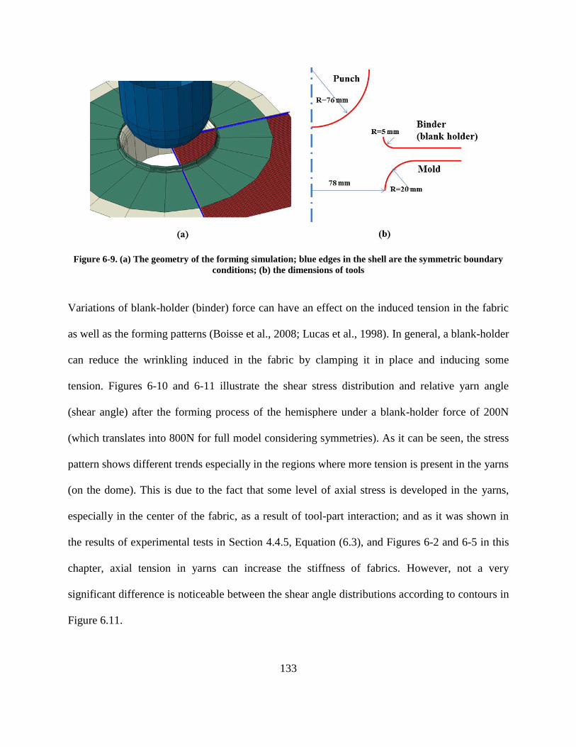
133
Figure 6-9. (a) The geometry of the forming simulation; blue edges in the shell are the symmetric boundary
conditions; (b) the dimensions of tools
Variations of blank-holder (binder) force can have an effect on the induced tension in the fabric
as well as the forming patterns (Boisse et al., 2008; Lucas et al., 1998). In general, a blank-holder
can reduce the wrinkling induced in the fabric by clamping it in place and inducing some
tension. Figures 6-10 and 6-11 illustrate the shear stress distribution and relative yarn angle
(shear angle) after the forming process of the hemisphere under a blank-holder force of 200N
(which translates into 800N for full model considering symmetries). As it can be seen, the stress
pattern shows different trends especially in the regions where more tension is present in the yarns
(on the dome). This is due to the fact that some level of axial stress is developed in the yarns,
especially in the center of the fabric, as a result of tool-part interaction; and as it was shown in
the results of experimental tests in Section 4.4.5, Equation (6.3), and Figures 6-2 and 6-5 in this
chapter, axial tension in yarns can increase the stiffness of fabrics. However, not a very
significant difference is noticeable between the shear angle distributions according to contours in
Figure 6.11.

134
It should be noted that although in most cases the final configuration of fabric (e.g., the relative
angle between warp and weft, and the final shape) would be of primary interest to manufacturers,
the general distribution of stresses and particularly the shear stress in the fabric can also be of
high importance to designers. More specifically, stresses developed in the fabric during the
forming stage can yield residual stresses in the final manufactured part. These stresses can play
even a more critical role when parts are prematurely de-molded. In industrial scale applications,
in order to increase the rate of production, parts are often de-molded before the resin is fully
consolidated. This is specially the case for the thermoset resins where a quite slow chemical
reaction needs to take place for full cure. It has been shown that due to the effect of the residual
stresses, if the part is de-molded prior to full consolidation of the resin, there can be noticeable
changes in its final shape (Komeili and Milani, 2013). Moreover, it has been shown that even
when a part has enough time for curing steadily inside the mold to an asymptotic level, during its
operational life if exposed to a temperature close to the material glass transition temperature, the
part may experience cure progression and, hence, cause further distortions due to original
residual stresses (Mohammadi et al., 2013).

135
Figure 6-10. Comparison of predicted shear stress in forming with a hemisphere punch using the uncoupled
and coupled models (units in Pa); a blank-holder force of 200N is used in the simulation
To
p v
iew
Isom
etric
view
Uncoupled
tension-shear
Coupled
tension-shear

136
Figure 6-11. Comparison of predicted relative/shear angle in forming with a hemisphere punch using the
uncoupled and coupled models (units in Radians); a blank-holder force of 200N is used in the simulation
In order to further study the effect of in-plane tension during hemisphere forming, another case
study with similar geometry and punch motion was run with lower blank force of 25N (which
translates into 100N for full model considering symmetries) and in-plane pre-tension of 400 N/m
along the free edges of the fabric. Results for in-plane shear stress and relative shear angle are
To
p v
iew
Isom
etric
view
Uncoupled
tension-shear
Coupled
tension-shear

137
demonstrated in Figures 6-12 and 6-13, respectively. As it can be seen in this case, despite
significant stress variations in the fabric especially closer to the center where there is more
tension, the deformation of the fabric in hemispherical punch still is not affected distinctly by the
coupling. Results of these two case studies on the forming of hemisphere can be related to the
fact that this forming process is dominated by the mold, punch and binder shape and is more or
less a displacement-controlled deformation. Therefore, although the level of predicted stress is
higher in shear-tension coupled model, it is not high enough to affect the distribution of shear
angle in the fabric. That is why previous models (even geometrical models for draping) were
able to capture the hemisphere draping of fabrics with high accuracy. In other words, this can be
related to the fact that the hemisphere mold does not have sharp corner features around which the
forming fabric could be more flexible to take an arbitrary shape inside the mold (this proposition
will be further investigated in the next examples). Almost regardless of stiffness of fabric, very
similar shapes were formed as final product in hemisphere forming process.

138
Figure 6-12. Comparison of the predicted shear stress in forming with a hemisphere punch using the
uncoupled and coupled models (units in Pa); a blank-holder force of 25N and pre-tensioning force of 400 N/m
are used in the simulation
To
p v
iew
Isom
etric
view
Uncoupled
tension-shear
Coupled
tension-shear

139
Figure 6-13. Comparison of the predicted relative/shear angle in forming with a hemisphere punch using the
uncoupled and coupled models (units in radians); a blank-holder force of 25 and pre-tensioning force of 400
N/m are used in the simulation
In order to gain a better insight into the deformation/shear angle pattern on the formed fabrics in
the present case study, the shear angle along a selected path line starting from center of the
hemisphere towards the corner point of fabric was extracted. The selected path line as well as
To
p v
iew
Isom
etric
view
Uncoupled
tension-shear
Coupled
tension-shear

140
values of shear angle distribution along the path is shown in Figure 6-14. As it can be seen, the
difference between models in various situations is more noticeable closer to the end of the path
line which is the area not bounded between punch and mold and fabric can move more freely.
Figure 6-14. The shear angle distribution along a selected path line in hemisphere forming: (a) the location of
line on the formed fabrics; (b) the values of shear angle along the line as a function of distance from the
center of hemisphere
Start point
0
0.1
0.2
0.3
0.4
0.5
0.6
0.7
0.8
0 0.02 0.04 0.06 0.08 0.1 0.12 0.14 0.16 0.18 0.2
Sh
ear
an
gle
(ra
dia
ns)
Distance from the center point (m)
(UnCoupled) Blank force 200 N
(UnCoupled)Blank force 25 N, PreTen 400 N/m
(Coupled)Blank force 200 N
(Coupled)Blank force 25 N, PreTen 400 N/m
(a)
(b)

141
Figure 6-15 shows a comparison between the shear angles predicted by the present model
(including the shear-tension interaction) and the results of a similar analysis conducted by
(Jauffres et al. 2011) without the coupling terms. The overall trend of the shear angle and the
final shape of the fabric show very similar trends. Next to the coupling effect, the small
variations in the predicted shear angles can be due to differences in the geometrical features,
range of legends, frictions and boundary conditions used in these two simulations.
Figure 6-15. Validating the forming model; (a) the shear angle (in radians) using the current coupled model;
(b) the shear angle (in degrees) using uncoupled model (Jauffrès et al., 2011)
6.4.2 Double dome benchmark forming
Double dome benchmark is another process studied by researchers as a benchmark for forming
simulation of woven fabrics (Boisse, 2010; Khan et al., 2010; Wonoh Lee et al., 2009; Sargent et
al., 2010). The tooling geometry is depicted in Figure 6-16 and includes more curvatures and
complex surfaces compared to the single dome hemisphere studied in Section 6.4.1. The

142
geometrical details of this model are accessible through woven fabric composites forum online
(www.wovencomposites.org). Because of the symmetry in the fabric, only a quarter of the fabric
is modeled and similar to the hemisphere forming case study, appropriate symmetry boundary
conditions are applied in the corresponding edges. All the details of tool-part interactions are
similar to the hemisphere case in Section 6.4.1.
Figure 6-16. The geometry of the double dome model; only a quarter of the fabric is simulated and symmetric
boundary conditions are applied at the blue highlighted edges of the fabric.
The first attempt was to simulate the above forming process with 100N (which corresponds to
400N for the full model) of blank-holder force and no fabric pretension on the free edges. The
corresponding shear stress and shear angle distributions in the fabric are demonstrated in Figures
6-17 and 6-18.
143
Figure 6-17. Comparison of the predicted shear stress in forming with a double dome punch and mold using
the uncoupled and coupled models (units in MPa); a blank-holder force of 100N is used in the simulation
To
p v
iew
Isom
etric
view
Uncoupled
tension-shear
Coupled
tension-shear

144
Figure 6-18. Comparison of the predicted shear/relative angle in forming with a double dome punch and
mold using the uncoupled and coupled models (units in radians); a blank-holder force of 100N is used in the
simulation
Again the stress trends are locally different in the coupled model compared to the uncoupled
model. Moreover, as it can be seen from the above figures, in this case there is more noticeable
Top
vie
wIso
metr
ic v
iew
Uncoupled
tension-shear
Coupled
tension-shear

145
difference between deformation patterns (relative angle between yarns) of the coupled and
uncoupled models of the fabric, when compared to hemisphere punch forming process. Although
the uncoupled model is still reasonably accurate in most of regions of the part, the highest
difference has occurred in the sharp corner of the formed fabric which corresponds to a zone
with a relatively high shear angle (the change in the relative angle between warp and weft).
Namely, the shear angle in this region is in the range of 0.8-0.9 radians. According to the
experiments conducted by Zhu et al. (2007b), the locking angle (side to side contact between
adjacent yarns), which can result in wrinkles in the fabric, starts around the shear angle of ~0.85
radians for this type of fabric. Thus, the comparison of the high shear angles in the present
forming simulation and the above experimental work would suggest that the use of the coupled
model may be more critical in predicting wrinkling defect in critical zones of the fabric during
forming.
Recalling Figure 6-5, it can also be mentioned that the differences in the fabric shear stress
response at different levels of yean tensioning are more noticeable when . When a
small amount of yarn tension is involved there should be no considerable difference between the
model that takes into account the coupling with the one that ignores the effect. In the punch
forming simulations, the axial strains induced inside the fabric are higher on the sharp corners
where the difference between the two models is also noticed. For example, Figure 6-19 shows
the distribution of the axial strain along weft ( ) in the double-dome forming case. As it can be
seen, the regions with higher amount of axial tension correspond to the regions in Figure 6-17
where the difference between the shear stress response of the uncoupled and coupled model is
apparent. The effect of shear-tension interaction is even clearer where higher shear angles are
involved. Indeed, according to the shear response surface in Figure 6-5a, the combination of high

146
shear angle and high axial strain along yarns can result in the most distinct predictions between
the coupled and uncoupled models during forming simulations. This combination is precisely
what is experienced by the fabric in the sharp corners during the double-dome forming process.
Figure 6-19. The axial strain along weft (ε2) in the double-dome forming case
A second example with this punch and mold was conducted with 10N blank-holder force (which
corresponds to 40N for the full model) along with a 400 N/m pre-tension along yarns on the free
edges of fabric. Results are illustrated in Figures 6-20 and 6-21.

147
Figure 6-20. Comparison of the predicted shear stress in forming with a double dome punch and mold using
the uncoupled and coupled models (units in MPa); a blank-holder force of 10N and pre-tensioning force of
400 N/m are used in the simulation
To
p v
iew
Isom
etric
view
Uncoupled
tension-shear
Coupled
tension-shear

148
Figure 6-21. Comparison of the predicted shear/relative angle in forming with a double dome punch and
mold using the uncoupled and coupled models (units in radians); a blank-holder force of 10N and pre-
tensioning force of 400 N/m are used in the simulation
As it can be seen from comparing figures that illustrate forming of the hemisphere to those for
the double-dome, the influence of the shear-tension coupling in the latter forming case is more
evident for both the predicted pattern of deformation and shear stress values. The reason can be
To
p v
iew
Isom
etric
view
Uncoupled
tension-shear
Coupled
tension-shear

149
related to the fact that the punch and mold in the double-dome forming process has more
geometrical features that fabric needs to be formed into, when compared to the hemisphere mold.
Therefore, the effect of locally higher axial tension and higher shear angle can play a more
important role in determining the final shape of the fabric. That is why the highest difference is
observed in the corner of the part (the red region in Figures 6-18 and 6-21), where the fabric is
formed around a sharp corner with a double curvature and more tension along warp and weft is
involved at the same time with a larger shear angle. This fact can also be noted quantitatively
from Figure 6-22 where the difference between various double dome forming conditions is more
emphasized compared to the hemisphere forming, especially on the regions far from the center.

150
Figure 6-22. The shear angle distribution along a selected path line in double dome forming: (a) the location
of line on the formed fabrics; (b) the values of shear angle along the line as a function of distance from the
start point
Start point
(a)
(b)
0
0.1
0.2
0.3
0.4
0.5
0.6
0.7
0.8
0.9
0 20 40 60 80 100 120 140 160 180
Sh
ear
an
gle
(ra
dia
ns)
Distance from the center point (mm)
(UnCoupled) Blank force 100 N
(UnCoupled)Blank force 10 N, PreTen 400 N/m
(Coupled)Blank force 100 N
(Coupled)Blank force 10 N, PreTen 400 N/m

151
Figure 6-23 illustrates a comparison between the predicted shear angle by the current coupled
model with 100 N blank-holder force (Figure 6-18) and the model used by (Peng and Rehman,
2011). While similarities between the tends of predicted shear angles and the final form of the
fabric are noticeable, the deviations in the magnitude of shear angles between the two studies can
be related to other differences in details of the modeling including the geometry of the blank-
holder, the friction coefficient, and the forces applied on the blank holder.
Figure 6-23. Validating the model; (a) the predicted shear angle (in radians) using the newly developed
model; (b) the predicted shear angle (in degrees) in the simulation conducted by (Peng and Rehman, 2011)
6.4.3 Tetrahedral punch forming
After simulating the fabric forming with a simple curvature (hemisphere punch) and a more
complicated case (double-dome punch and mold) it was realized that the effect of including
shear-tension can have a better pay-off for accuracy in regions where fabric can move more
freely and around sharp corners. Thus, a third case study for forming of a very sharp corner,
which includes both of these features, was considered. Indeed, the manufacturing of a tetrahedral

152
shape with punching is a complicated forming process, and one that is prone to occurrence of
several defects. As a step to explore application of fabrics in manufacturing this type of parts,
and also to evaluate the capabilities of numerical methods for predicting their underlying
forming pattern, the forming study of woven fabrics using a tetrahedral shape punch has been
explored recently by researchers (Allaoui et al., 2011; Hamila et al., 2009; Hivet et al., 2009). A
similar case study with geometrical details shown in Figure 6-24 was studied here.
Figure 6-24. The geometry of tetrahedral punch and fabric
Details of the FE model and fabric-tool interaction are similar to two previously studied forming
cases in this chapter (hemisphere and double-dome forming). This time, however, there is only
one plane of symmetry. Thus, only half of the fabric is modeled and appropriate symmetry
boundary conditions were applied on the corresponding edges. Results for a blank-holder force
of 200 N (which corresponds to 400N for the full model) are illustrated in Figures 6-25 and 6-26.
80
75
40
200
Blank-holders
Punch

153
Figure 6-25. Comparison of the predicted shear stress in forming with a tetrahedral punch using the
uncoupled and coupled models (units in Pa); a blank-holder force of 200N is used in the simulation
To
p v
iew
Isom
etric
view
Uncoupled
tension-shear
Coupled
tension-shear

154
Figure 6-26. Comparison of the predicted shear/relative angle in forming with a tetrahedral punch using the
uncoupled and coupled models (units in radians); blank-holder force of 200N is used in the simulation
As it can be seen in this case, similar to the forming of the hemisphere, significant differences
are observed in terms of the shear stress distributions between the coupled and the uncoupled
models, where the shear angle distributions do not show noticeable differences. This can be
related back to the fact that there is not much tension involved along warp and weft in this
Top
vie
wIso
metric
vie
w
Uncoupled
tension-shear
Coupled
tension-shear

155
forming process and therefore the shear stiffness is not affected by the coupling effect enough to
develop a distinct distribution of shear angle in the formed fabric.
Next, similar to previous cases the effect of pre-tensioning on the fabric was studied by keeping
the same blank force and adding a pre-tension force of 400 N/m on the free edges of the fabric.
Results are illustrated in Figures 6-27 and 6-28.
Figure 6-27. Comparison of the predicted shear stress in forming with a tetrahedral punch using the
uncoupled and coupled models (units in Pa); blank-holder force of 200N and pre-tensioning force of 400 N/m
are used in the simulation
Top
vie
wIso
metric
vie
w
Uncoupled
tension-shear
Coupled
tension-shear

156
Figure 6-28. Comparison of the predicted shear/relative angle in forming with a tetrahedral punch using the
uncoupled and coupled models (units in radians); a blank-holder force of 200N and pre-tensioning force of
400 N/m are used in the simulation
As it can be seen from comparing Figure 6-27, again the shear stress trend is noticeably affected
by including the coupling/interaction that exists between shear and tension using the model
Top
vie
wIso
metric
vie
w
Uncoupled
tension-shear
Coupled
tension-shear
157
developed in this thesis. However, from Figure 6-28 the shear angle distribution is fairly
comparable between coupled and decoupled models. Figure 6-29 shows a path line along the
edge of the deformed fabric in this molding configuration and the corresponding distributions of
the shear angle using uncoupled and coupled models in two different forming scenarios (i.e.,
with or without shear pre-tension). As it can be seen in the figure, the deformation difference
between the two scenarios is quite evident especially for regions away from the punch and closer
to the free edges of the fabric. The interesting point in this simulation compared to the double-
dome forming was that within each scenario, the effect of including the shear-tension coupling
could make more clear difference between results in the double-dome forming case. This
suggests the fact that the presence of only one sharp corner may not affect the overall formation
of shear angle in a fabric. The effect of increase in shear stiffness from tension depends on the
whole geometry of the mold and punch and the resulting local formation of fabric regions with
different geometrical features.

158
Figure 6-29. The shear angle distribution along a selected path line in tetrahedral forming: (a) the location of
line on the formed fabrics; (b) the values of shear angle along the line as a function of distance from the start
point
Start point
(a)
(b)-1.2
-1
-0.8
-0.6
-0.4
-0.2
0
0.2
0.4
0.6
0.8
0 0.02 0.04 0.06 0.08 0.1
Sh
ear
an
gle
(ra
dia
ns)
Distance from the center point (m)
(UnCoupled) Blank force 200 N
(UnCoupled)Blank force 200 N, PreTen 400 N/m
(Coupled)Blank force 200 N
(Coupled)Blank force 200 N, PreTen 400 N/m

159
6.4.4 Concluding remarks on forming simulations with tension-shear coupling
Three different forming processes for manufacturing of hemisphere, double dome and tetrahedral
shapes with sharp corners were studied in Sections 6.4.1 to 6.4.3 and the general conclusion was
that including the interaction between shear and tension affects the shear stress distribution in the
fabric considerably. The distribution of stresses induced during the forming process of fabrics
can have an effect on the final product performance after curing the composite and de-molding
(Komeili & Milani, 2013).
It was reported that the effect of coupling in the current case studies does not influence the
overall shear angle deformation in most cases. This is due to the fact that the levels of tensioning
in most of the forming regions are not high enough to distinguish the results between the coupled
model and the uncoupled model. However, in some particular regions where the fabric in fact
goes under high amount of in-plane tension along warp and weft (such as the sharp corner that
was noticed in the double-dome case study), there is a noticeable difference between the shear
angles predicted with the coupled model compared to the uncoupled model. What makes this
observation more interesting is that this deviation on the above mentioned region has happened
in a shear angle which is close to the locking angle of this particular fabric (TWINTEX plain
weave). Therefore, having a reliable prediction of shear angle on these critical regions can be of
high interest.
On the other hand, the inherent uncertainties that exist in fabrics such as yarn dimensional
variations and misalignment (Abdiwi et al., 2012; Komeili & Milani, 2010) may have similar or
even more effect on the forming quality of a final product. In practice, they can add to the effect
of coupling. For example, it is reported that during the shear frame test the misalignment of the
fibers can induce excessive tension in the fabric (Milani et al., 2007). Using the uncoupled model
160
the effect of this interaction on the shear stiffness cannot be taken into account, whereas the
coupled model can be more accurate in predicting the real amount of shear stress and separating
it from the tensile stresses due to yarn extension. Similarly in forming complex geometries if the
fabric is aligned in a direction exerting high amounts of tension along yarns, the effect of
increase in the shear stiffness and its influence on the final shape of the part can be taken into
account more closely via the coupled model.
One of the other facts about the studied punching processes was that they are normally
displacement-controlled. In other words, the geometry of the mold and punch does not allow the
fabric to have a flexible shape to form into; fabric is draped by punch into the mold shape
regardless of its stiffness. Therefore, changes in shear stiffness due to tension which was of the
order of 30-50% can only affect the stress/force response. However, studying the deformation on
local regions that are allowed to deform more freely (areas that are not squeezed into mold by
punch; such as those closer to blank holder) and some critical regions around sharp corners
provided some different results using the coupled model. In particular, among the punches
studied, the first two had large forming areas under the punch, and also due to the geometry of
blank-holder in the hemisphere case and constraints of mold and punch in the double dome case,
there was not much out-of-plane wrinkling even in the absence of fiber tensioning. However,
studying the out of plane displacement (u3) of the fabric in the tetrahedral forming at the areas far
from punch showed formation of regions with out of plane waviness in the fabric which could
point to the presence and onset of wrinkles (see Figure 6-30), especially when the fabric is under
initial tension.

161
Figure 6-30. The out of plane displacement of the fabric (representing wrinkles) in the tetrahedral forming
predicted from the uncoupled model in comparison to the coupled model
6.5 Summary
In this chapter the meso-level model characterized in the previous chapter was used to generate
response surfaces for stress response of the TWINTEX plain woven fabric under general in-
plane deformation modes. Then the stress behavior equations were used to predict the response
Bla
nk
force : 2
00 N
No
prete
nsio
n
Uncoupled
tension-shear
Coupled
tension-shear
Bla
nk
force
: 20
0 N
Pre-ten
sion
: 40
0 N
/m

162
of an inflatable composite structure (shaft) to twisting moment. A noticeable difference was
found between predictions of the old model (with no shear-tension coupling) and the new
coupled model. Then Abaqus finite element software was used along with its fabric material
model to simulate forming with three different shapes. It was found that, although the decoupled
model seems to be decently accurate in predicting the global shear angle distribution in most
forming cases (which is due to displacement-controlled nature of the studied punching
processes), more clear differences can be observed in terms of shear stress, local shear angle on
critical regions around sharp corners as well as wrinkling pattern which can in turn justify
characterizing coupled models for design of advanced parts.

163
Chapter 7: Summary, Conclusions, and Future work
7.1 Summary
Despite their popularity and wide applications, simulation models of textile composites are sill
not as advanced as conventional materials such as metals, polymers and unidirectional
composites. This lack of knowledge is mainly related to the inherent heterogeneity and multi-
scale nature of textile composites with complex fibrous architectures. In the case of woven
fabrics, a part formed at the macro-level is made of several yarn subsystems at meso-level which
are in turn made of micro-level fiber substructures. The complexity of interactions between
different elements in different scales/levels makes the behavior of woven fabrics complicated to
characterize using conventional mechanical tests and simulation models.
Low in-plane shear stiffness of woven fabrics is known to be one of their important properties
providing them with a superior formability. Therefore, understanding shear stiffness of fabrics is
crucial in studying their deformation and forming processes. There have been several attempts in
characterizing the shear response of woven materials using different tests such as bias-extension
and shear frame tests. Despite benefits and drawbacks of each method, one important question
has been, “Is the fabric shear stiffness an independent material property and only a function of
shear angle?” Although in most past research this stiffness was assumed to be an independent
property and a function of shear strain (relative angle between warp and weft yarns), recent
evidences from experiments as well as simplified numerical simulations pointed that in fact there
can be a strong dependency between shear stiffness and tensile properties along yarns in woven
fabrics. Hence, to enhance the reliability of numerical simulation of fabric forming processes, the
research motivation for this thesis was a full characterization of shear-tension coupling in dry
woven fabrics.

164
Two approaches were possible for studying and characterizing the coupling phenomenon. First
one was based on designing a new test fixture capable of inducing mixed mode deformations
(axial tension + in-plane shear) in a controlled manner, and the second one was proposing a
virtual experimentation technique. While some advances in the former approach was made in
this research, it still requires further fixture design modifications and calibration with standard
tests such biaxial tension and shear frame. The latter approach, which formed the bulk of the
research, required a fully characterized meso-level (yarn) model to extract macro-level (fabric)
material response under combined loading modes. Choosing a typical dry woven composite
(TWINTEX®
plain weave fabric), it was shown that physically separating meso-level elements
(yarns) from the whole system (fabric) and running tensile and shear experiments on individual
yarns is not practical, due to variability and induced damage/local crimping in yarns during each
extraction. Therefore, a new multi-objective inverse identification method was proposed to
determine material properties of yarns at meso-level. Finite element-based inverse identification
methods in general are based on the principles of curve fitting, where the difference between
model predictions and experimental data are minimized. In multi-objective identification,
however, errors corresponding to multiple deformation modes should be minimized
simultaneously. In order to retain the finite element model suitable for simulating general in-
plane deformations (i.e., relevant to actual forming processes), two different characterization
experiments were selected during inverse identification. Namely, uni-axial tension along yarns
and shear frame (trellis) deformation after pre-tensioning were conducted on fabric samples and
used as the input data for inverse identification of yarn constitutive model constants. Multi-
objective genetic algorithm tool was used to run the inverse identification and minimize the error
between predictions of meso-level models and the macro-level experimental data.

165
Having identified the material properties of yarns, the meso-level finite element model was run
in a 10-level full factorial design under all different combinations of axial tensions along warp
and weft as well as different shear angles. A response surface was then extracted based on a
polynomial function of tensile and shear strains, which could accurately reproduce the original
full-factorial data. Primarily results showed (a) a strong dependency of shear stiffness on axial
tension of yarns, but (b) a low contribution of shear on the axial response of the fabric along
yarns. Moreover, it was shown than there is a high level of non-linearity in the response of fabric
under combined loading, which can make the deformation dependent on the sequence of the
deformation modes. In other words, the sequence of applying the shear and tension (under
identical levels of deformation) can lead to different deformation histories. However, this level
of nonlinearity due to loading sequence is neglected at the moment and the polynomial stress
response mentioned above was selected as the general material response under simultaneous
shear-tension loading (which would be more common in practical applications).
The characterized macro-level material behavior was then used in applications of woven fabrics
in two ways. First an analytical closed-form formula was driven from the identified response
surface and used for studying inflatable woven fabric beams under torsional loading. Second, a
series of finite element simulation of different stamp forming processes were presented for the
same fabric. It was observed that in the case of inflatable beams, the structure’s torsional
performance can be up to 5% different using old (un-coupled) method compared to the newly
developed coupled model.
For forming process simulations, the non-orthogonal material behavior of dry fabrics was
handled in Abaqus using the built-in fabric material model which was customized via
FORTRAN subroutine of vfabric in order to embed the identified stress response surface under

166
shear-tension coupling. Three different benchmark forming cases including hemisphere, double
dome and tetrahedral shapes were used as case studies. Results of simulations for this particular
fabric showed that in general, although the level of predicted shear stress in the coupled model is
higher than the un-coupled model, the overall deformation patterns (particularly relative angle
between yarns) are not significantly affected, except for some critical regions of the part with
complex geometrical features such as sharp corners or double curvature. The high level of axial
strain along yarns and shear angle are the reasons that considerable deviation happens in these
particular regions of the fabric, whereas in most of other regions the level of axial strain and
shear angle is not high enough for the coupled model to be distinguishable from the uncoupled
model. However, design point of view, these sharp corner regions are practically critical zones
where fabric is susceptible to failure or wrinkles. Moreover, for some forming shapes, such as
tetrahedral case, waviness forming in regions away from the punch showed very different
patterns using uncoupled versus coupled models. Nonetheless, for a small amount of tensile
force along the yarns and simple geometries (such as hemisphere), the conventional decoupled
models can be accurate enough to predict the overall form of the part and global shear angle
response, especially considering the high level of variability that exists within the fabric
properties itself. The stress response can however be notably different between the two models.
Moreover, for complex shapes (e.g., with sharp corners) and/or advanced quality measures such
as local wrinkles, the effect of shear-tension coupling should be taken into account.
7.2 Conclusions
The main findings and contributions of the presented thesis, following the same order of the
objectives defined in Section 1.6, can be summarized as follows.

167
1. A new test device was designed for studying in-plane pin-joint shear (trellising)
deformation of fabrics under simultaneous axial tension along yarns. The device is also
capable of applying a newly defined mode of shear, known as sliding shear, which has
different kinematics than trellising mode. Virtual experimentation was suggested as an
alternative method to reduce the high cost of experiments. However, a careful multi-
objective inverse identification along with macro-level testing using existing benchmark
fixtures were required to characterize the model constants for yarns within the fabric
material system. During multi-objective optimization, the Pareto curves can assist the
analysis to adjust the weighing factor between different deformation modes.
2. The general stress response function of the dry TWINTEX® plain-weave fabric was
extracted via virtual experiments at meso-level in conjunction with full-factorial design
of experiment (DOE) methodology under different combinations of yarn tension and in-
plane trellis shear levels. The material properties of yarns were characterized using the
multi-objective inverse identification. Results proved that there is a strong dependency of
the fabric shear stiffness on tensile stiffness of yarns, and not vice versa.
3. Two sets of case studies were investigated to further understand the effect of shear-
tension interaction in practical applications:
(i) Using the characterized model with shear-tension interaction, the
response of inflatable structures made of woven fabrics was analyzed and
results were compared to the earlier (un-coupled) models. Up to 5%
difference can be observed between these two approaches due to the
coupling.

168
(ii) Forming process of hemisphere, double dome and tetrahedral shapes was
investigated for the first time using a coupled non-orthogonal fabric
model in Abaqus which was customized for the proposed model via a
vfabric subroutine. Results indicated that generally both coupled and
uncoupled models can predict the overall deformation patterns accurately;
however, the coupled model can be superior in predicting the shear angle
in critical zones of formed part with complex curvatures as well as
waviness developed in the free surfaces of the fabric. Also, the level of
stresses that material undergoes was found to be more accurate in the
coupled model, which can be important for estimating residual stresses in
composites.
7.3 Future work
For potential future work, the response surface generated in this research by virtual
experimentation can be further validated through physical experiments using the newly
developed combined loading test fixture. This can be done using both sequential and
simultaneous loading scenarios, and subsequently new state variables may be introduced to the
response surface to take into account the dependency of fabric behavior on the loading history.
The study of fabric response under general in-plane loadings at high temperatures, or during
curing process of composite parts, can also be a very worthwhile future research topic.
Moreover, similar experiments can be conducted on other types of fabric architecture and fiber
materials to investigate the generalization of current conclusions.

169
Problems reported by advanced manufacturers during forming of textile composites indicate that
wrinkling is one of the main forms of defects; since it can result in deterioration of mechanical
properties of the final part and its quality. This problem becomes even more sophisticated when
forming multi-layer composites under interactions effect both within and between layers.
Occurrence of locking and formation of wrinkles in the critical zones should be studied in more
details via the coupled model developed here.

170
Bibliography
Abbott, G. M., Grosberg, P., & Leaf, G. A. V. (1971). The Mechanical Properties of Woven
Fabrics: Part VII: The Hysteresis During Bending of Woven Fabrics. Textile Research
Journal, 41(4), 345–358.
Abdiwi, F., Harrison, P., Koyama, I., Yu, W. R., Long, a. C., Corriea, N., & Guo, Z. (2012).
Characterising and modelling variability of tow orientation in engineering fabrics and
textile composites. Composites Science and Technology, 72(9), 1034–1041.
Abdiwi, F., Harrison, P., & Yu, W. R. (2013). Modelling the Shear-Tension Coupling of Woven
Engineering Fabrics. Advances in Materials Science and Engineering, 2013, 1–9.
Allaoui, S., Boisse, P., Chatel, S., Hamila, N., Hivet, G., Soulat, D., & Vidal-Salle, E. (2011).
Experimental and numerical analyses of textile reinforcement forming of a tetrahedral
shape. Composites Part A: Applied Science and Manufacturing, 42(6), 612–622.
ASTM. (2011). ASTM D5035-11: Standard test method for breaking force and elongation of
textile fabrics (strip method).
Badel, P., Gauthier, S., Vidal-Sallé, E., & Boisse, P. (2009). Rate constitutive equations for
computational analyses of textile composite reinforcement mechanical behaviour during
forming. Composites Part A: Applied Science and Manufacturing, 40(8), 997–1007.
Badel, P., Vidal-Salle, E., & Boisse, P. (2007). Computational determination of in-plane shear
mechanical behaviour of textile composite reinforcements. Computational Materials
Science, 40(4), 439–448.
Badel, P., Vidal-Salle, E., & Boisse, P. (2008). Large deformation analysis of fibrous materials
using rate constitutive equations. Computers & Structures, 86(11-12), 1164–1175.
Badel, P., Vidal-Salle, E., Maire, E., & Boisse, P. (2008). Simulation and tomography analysis of
textile composite reinforcement deformation at the mesoscopic scale. Composites Science
and Technology, 68(12), 2433–2440.
Bakhvalov, N., & Panasenko, G. (1989). Homogenisation: averaging processes in periodic
media: mathematical problems in the mechanics of composite materials. Boston: Kluwer
academic publisher.
Ballhause, D., König, M., & Kröplin, B. (2005). A microstructure model for fabric-reinforced
membranes based on discrete element modelling. In International conference on Textile
Composites and Inflatable Structures. Barcelona: CIMNE.
Ballhause, D., Konig, M., Kroplin, B., & Source, C. (2006). Modelling of woven fabrics with the
Discrete Element Method. In European Conference on Computational Mechanics. Lisbon,
Portugal.
Bassett, R. J., Postle, R., & Pan, N. (1999). Experimental Methods for Measuring Fabric
Mechanical Properties: A Review and Analysis. Textile Research Journal, 69(11), 866–875.
Beer, F. P., Johnston, E. R., DeWolf, J. T., & David, M. F. (2009). Mechanics of Material (5th
ed.). Singapore: McGraw-Hill Higher Education.

171
Benboubaker, B., Haussy, B., & Ganghoffer, J. (2007). Discrete models of woven structures.
Macroscopic approach. Composites Part B: Engineering, 38(4), 498–505.
Bhatti, A. (Ed.). (2008). Stereo Vision. InTech. doi:10.5772/89
Boisse, P, Gasser, A., & Hivet, G. (2001). Analyses of fabric tensile behaviour: determination of
the biaxial tension–strain surfaces and their use in forming simulations. Composites Part A:
Applied Science and Manufacturing, 32(10), 1395–1414.
Boisse, P, Zouari, B., & Gasser, A. (2005). A mesoscopic approach for the simulation of woven
fibre composite forming. Composites Science and Technology, 65(3-4), 429–436.
Boisse, P., Borr, M., Buet, K., & Cherouat, A. (1997). Finite element simulations of textile
composite forming including the biaxial fabric behaviour. Composites. Part B, Engineering,
28(4), 453–464.
Boisse, P., Buet, K., Gasser, A., & Launay, J. (2001). Meso/macro-mechanical behaviour of
textile reinforcements for thin composites. Composites Science and Technology, 61(3),
395–401.
Boisse, P., Hamila, N., Helenon, F., Hagege, B., & Cao, J. (2008). Different approaches for
woven composite reinforcement forming simulation. International Journal of Material
Forming, 1(1), 21–29.
Boisse, P., Hamila, N., Vidal-Sallé, E., & Dumont, F. (2011). Simulation of wrinkling during
textile composite reinforcement forming. Influence of tensile, in-plane shear and bending
stiffnesses. Composites Science and Technology, 71(5), 683–692.
Boisse, Philippe. (2006). Meso-macro approach for composites forming simulation. Journal of
Materials Science, 41(20), 6591–6598.
Boisse, Philippe. (2010). Simulations of Woven Composite Reinforcement Forming. In Woven
Fabric Engineering (pp. 387–414). InTech.
Boisse, Philoppe, Hamila, N., Wang, P., Gatouillat, S., & Charmetant, A. (2011). Composite
Reinforcement Forming Simulation : Continuous And Mesoscopic Approaches. In 18th
International Conference On Composite Materials (pp. 1–6). Jeju, South Korea.
Breen, D. E., House, D. H., & Getto, P. H. (1992). A physically-based particle model of woven
cloth. The Visual Computer, 8(5-6), 264–277.
Buet-Gautier, K., & Boisse, P. (2001). Experimental analysis and modeling of biaxial
mechanical behavior of woven composite reinforcements. Experimental Mechanics, 41(3),
260–269.
Cai, Z., Yu, J. Z., & Ko, F. K. (1994). Formability of textile preforms for composite applications.
Part 2: Evaluation experiments and modelling. Composites Manufacturing, 5(2), 123–132.
Cao, J., Akkerman, R., Boisse, P., Chen, J., Cheng, H., Degraaf, E., Gorczyca, J., Harrison, P.,
Hivet, G., & Launay, J. (2008). Characterization of mechanical behavior of woven fabrics:
Experimental methods and benchmark results. Composites Part A: Applied Science and
Manufacturing, 39(6), 1037–1053.

172
Cavallaro, Paul V, Sadegh, A. M., & Quigley, C. J. (2006). Bending Behavior of Plain-Woven
Fabric Air Beams : Fluid-Structure Interaction Approach. Technical report: Naval
Undersea Warfare Center Division New Port, Rhode Island.
Cavallaro, Paul V, Sadegh, A. M., Quigley, C. J., & Johnson, A. R. (2004). Effects of Coupled
Biaxial Tension and Shear Stresses on Decrimping Behavior in Pressurized Woven Fabrics.
Technical report: Naval Undersea Warfare Center Division New Port, Rhode Island.
Cavallaro, P. V., Sadegh, A. M., & Quigley, C. J. (2007). Decrimping Behavior of Uncoated
Plain-woven Fabrics Subjected to Combined Biaxial Tension and Shear Stresses. Textile
Research Journal, 77(6), 403–416.
Cavallaro, Paul V., Johnson, M. E., & Sadegh, A. M. (2003). Mechanics of plain-woven fabrics
for inflated structures. Composite Structures, 61(4), 375–393.
Charmetant, a., Vidal-Sallé, E., & Boisse, P. (2011). Hyperelastic modelling for mesoscopic
analyses of composite reinforcements. Composites Science and Technology, 71(14), 1623–
1631.
Chen, J., & Prodromou, A. G. (1997). On the relationship between shear angle and wrinkling of
textile composite preforms. Composites Part A, 491–503.
Cherouat, A., & Billoe, J. L. (2001). Mechanical and numerical modelling of composite
manufacturing processes deep-drawing and laying-up of thin pre-impregnated woven
fabrics. Journal of Materials Processing Technology, 118, 460–471.
Chou, T., & Ko, F. (Eds.). (1989). Composite Material Series: Textile structural composites
(Vol. 3). Amsterdam: Elsevier.
Collier, J., Collier, B., O’Toole, G., & S.M., S. (1991). Drape prediction by means of finite-
element analysis. Journal of the Textile Institute, 82(1), 96–107.
Dong, L., Lekakou, C., & Bader, M. (2000). Solid-mechanics finite element simulations of the
draping of fabrics: a sensitivity analysis. Composites Part A: Applied Science and
Manufacturing, 31(7), 639–652.
Dridi, S., Morestin, F., & Dogui, a. (2012). Use of Digital Image Correlation to Analyse the
Shearing Deformation in Woven Fabric. Experimental Techniques, 36(5), 46–52.
Durville, D. (2007). Finite element simulation of textile materials at mesoscopic scale. In
Proceedings of the symposium ‘Finite element modelling of textiles and textile composites.
St. Petersburg.
Durville, Damien. (2005). Approach of the constitutive material behaviour of textile composites
through simulation. In International conference on Textile Composites and Inflatable
Structures. France.
Durville, Damien. (2008). Finite Element Simulation of the Mechanical Behaviour of Textile
Composites at the Mesoscopic Scale of Individual Fibers. In E. Oñate & B. Kröplin (Eds.),
Textile Composites and Inflatable Structures II. Netherlands.
Felippa, C. A. (2001). Nonlinear Finite Element Methods. Boulder, Colorado: University of
Colorado.

173
Fetfatsidis, K. a., Jauffrès, D., Sherwood, J. a., & Chen, J. (2011). Characterization of the
tool/fabric and fabric/fabric friction for woven-fabric composites during the
thermostamping process. International Journal of Material Forming.
Fish, J., & Belytschko, T. (2007). A First Course in Finite Elements. Chichester, UK: John
Wiley & Sons, Ltd.
Freeston, W. D., Platt, M. M., & Schoppee, M. M. (1967). Mechanics of Elastic Performance of
Textile Materials: Part XVIII. Stress-Strain Response of Fabrics Under Two-Dimensional
Loading1. Textile Research Journal, 37(11), 948–975.
Gasser, A., Boisse, P., & Hanklar, S. (2000). Mechanical behaviour of dry fabric reinforcements.
3D simulations versus biaxial tests. Computational Materials Science, 17(1), 7–20.
Gatouillat, S., Vidal-Sallé, E., & Boisse, P. (2010). Advantages of the Meso/Macro Approach for
the Simulation of Fibre Composite Reinforcements. International Journal of Material
Forming, 3(S1), 643–646.
Green, A. E., & Naghdi, P. M. (1965). A general theory of an elastic-plastic continuum. Archive
for rational mechanics and analysis, 18(4).
Grosberg, P. (1966). The Mechanical Properties of Woven Fabrics Part II: The Bending of
Woven Fabrics. Textile Research Journal, 36(3), 205–211.
Grosberg, P., & Kedia, S. (1966). The Mechanical Properties of Woven Fabrics: Part I: The
Initial Load Extension Modulus of Woven Fabrics. Textile Research Journal, 36(1), 71–79.
Grosberg, P., Leaf, G. a. V., & Park, B. J. (1968). The Mechanical Properties of Woven Fabrics:
Part VI: The Elastic Shear Modulus of Plain-Weave Fabrics. Textile Research Journal,
38(11), 1085–1100.
Grosberg, P., & Park, B. J. (1966). The Mechanical Properties of Woven Fabrics: Part V: The
Initial Modulus and the Frictional Restraint in shearing of Plain Weave Fabrics. Textile
Research Journal, 36(5), 420–431.
Grosberg, P., & Swani, N. M. (1966a). The Mechanical Properties of Woven Fabrics: Part IV:
The Determination of the Bending Rigidity and Frictional Restraint in Woven Fabrics.
Textile Research Journal, 36(4), 338–345.
Grosberg, P., & Swani, N. M. (1966b). The Mechanical Properties of Woven Fabrics: Part III:
The Buckling of Woven Fabrics. Textile Research Journal, 36(4), 332–338.
Haas, R., & Dietzius, A. (1918). The stretching of the fabric and the deformation of the envelope
in nonrigid balloons. NACA Technical Report.
Hamila, N, & Boisse, P. (2008). Simulations of textile composite reinforcement draping using a
new semi-discrete three node nite element. Composites Part B: Engineering, 39(6), 999–
1010.
Hamila, N, Boisse, P., Sabourin, F., & Brunet, M. (2009). A semi-discrete shell finite element for
textile composite reinforcement forming simulation. International Journal for Numerical
Methods in Engineering, 79(12), 1443–1466.

174
Hamila, N., A., K., Gatouillat, S., De Luycker, E., Vidal-Sallé, E., Mabrouki, T., & Boisse, P.
(2011). Composite Reinforcement Forming Simulation : A Multiscale Approach. In 18th
International conference on composite materials. Jeju, South Korea.
Hamila, Nahiène, & Boisse, P. (2007). A Meso–Macro Three Node Finite Element for Draping
of Textile Composite Preforms. Applied Composite Materials, 14(4), 235–250.
Hancock, S. G., & Potter, K. D. (2006). The use of kinematic drape modelling to inform the hand
lay-up of complex composite components using woven reinforcements. Composites Part A:
Applied Science and Manufacturing, 37(3), 413–422.
Harrison, P., Abdiwi, F., Guo, Z., Potluri, P., & Yu, W. R. (2012). Characterising the shear–
tension coupling and wrinkling behaviour of woven engineering fabrics. Composites Part
A: Applied Science and Manufacturing, 43(6), 903–914.
Harrison, P., Clifford, M. J. J., & Long, A. C. C. (2004). Shear characterisation of viscous woven
textile composites: a comparison between picture frame and bias extension experiments.
Composites Science and Technology, 64(10-11), 1453–1465.
Harrison, P., Wiggers, J., & Long, A. C. (2008). Normalization of Shear Test Data for Rate-
independent Compressible Fabrics. Journal of Composite Materials, 42(22), 2315–2344.
Healy, B., & Dodds, R. (1992). A large strain plasticity model for implicit finite element
analyses. Computational mechanics, 9(2), 95–112.
Hivet, G., Allaoui, S., Soulat, D., Wendling, A., Chatel, S., Works, I., & Modelling, M. (2009).
Analysis of woven reinforcement preforming using an experimental approach. In
Proceedings of the 17th International Conference on Composite Materials. Edinburgh, UK.
Hivet, G., & Boisse, P. (2005). Consistent 3D geometrical model of fabric elementary cell.
Application to a meshing preprocessor for 3D finite element analysis. Finite Elements in
Analysis and Design, 42(1), 25–49.
Holzapfel, G. A. (2000). Nonlinear solid mechanics: a continuum approach for engineering.
John Wiley & Sons Ltd.
Hu, J. (2004). Structure and mechanics of woven fabrics. Cornwall, England: Woodhead
Publishing Ltd and CRC Press LLC.
CMH-17. (2012). Composite Materials Handbook, Volume 1. SAE International.
Jauffrès, D., Sherwood, J. A., Morris, C. D., & Chen, J. (2010). Discrete mesoscopic modeling
for the simulation of woven-fabric reinforcement forming. International Journal of
Material Forming, 3(S2), 1205–1216.
Jaumann, G. (1911). Geschlossenes System physikalischer und chemischer Differentialgesetze.
Sitzgsber. Akad. Wiss. Wien (IIa).
Kaw, A. K. (1997). Mechanics of composite materials. New York: CRC Press.
Kawabata, S., Niwa, M., & Kawai, H. (1973a). Finite-deformation theory of plain-weave fabrics
- 1. The biaxial-deformation theory. Journal of the Textile Institute, 64, 21–46.
Kawabata, S., Niwa, M., & Kawai, H. (1973b). Finite-deformation theory of plain-weave fabrics
- 2. The uniaxial-deformation theory. Journal of the Textile Institute, 64, 47–61.

175
Kawabata, S., Niwa, M., & Kawai, H. (1973c). Finite-deformation theory of plain-weave fabrics
- 3. The shear-deformation theory. Journal of the Textile Institute, 64, 62–85.
Khan, M. a., Mabrouki, T., Vidal-Sallé, E., & Boisse, P. (2010). Numerical and experimental
analyses of woven composite reinforcement forming using a hypoelastic behaviour.
Application to the double dome benchmark. Journal of Materials Processing Technology,
210(2), 378–388.
Komeili, M, & Milani, A. (2013). An elaboration on the shear characterization of dry woven
fabrics using trellising tests. Polymer Composites, 34(3), 359–367.
Komeili, M, & Milani, A. S. (2011). A comparison of implicit and explicit finite element
methods for the meso-level simulation of dry woven fabric composites. In 18th
International conference on composite materials. Jeju, South Korea.
Komeili, M., & Milani, A. S. (2010). Meso-Level Analysis of Uncertainties in Woven Fabrics.
VDM Verlag Dr. Muller GmbH & C. KG.
Komeili, M., & Milani, A. S. (2011). Finite Element Modeling of Woven Fabric Composites at
Meso-Level Under Combined Loading Modes. In S. Vassiliadis (Ed.), Advances in Modern
Woven Fabrics Technology. InTech.
Komeili, M., & Milani, A. S. (2012). Inverse identification of meso-level material properties in
woven fabrics using multi-objective optimization. In 15th European Conference on
Composite Materials. Venice, Italy.
Komeili, M., & Milani, A. S. (2013). Solid Mechanics-based Simulation of Composite Forming
with Stress Relaxation in the Dry Fabric Reinforcement and Resin Curing. In 19th
international conference on composite materials (ICCM19). Montreal, Canada.
Lampinen, J. (2000). Multiobjective Nonlinear Pareto-Optimization. Lappeenranta university of
technology.
Lancaster, P., & Tismenetsky, M. (1985). The theory of matrices: with applications. Acadenic
press.
Launay, J, Hivet, G., Duong, A., & Boisse, P. (2008). Experimental analysis of the influence of
tensions on in plane shear behaviour of woven composite reinforcements. Composites
Science and Technology, 68(2), 506–515.
Launay, Jean, Hivet, G., Vu Duong, A., & Boisse, P. (2007). Experimental analysis of in plane
shear behaviour of woven composite reinforcements. Influence of tensions. In AIP
Conference Proceedings (pp. 1033–1038). AIP.
Lebrun, G., Bureau, M., & Denault, J. (2003). Evaluation of bias-extension and picture-frame
test methods for the measurement of intraply shear properties of PP/glass commingled
fabrics. Composite Structures, 61(4), 341–352.
Lee, W., Byun, J. H., Um, M. K., Cao, J., & Boisse, P. (2009). Coupled Non-orthogonal
Constitutive Model For Woven Fabric Composites. In 17th International Conference on
Composite Materials. Edinburgh.
176
Lee, Wonoh, Um, M., Byun, J., Boisse, P., & Cao, J. (2009). Numerical study on thermo-
stamping of woven fabric composites based on double-dome stretch forming. International
Journal of Material Forming, 3(S2), 1217–1227.
Li, S., Zhou, C., Yu, H., & Li, L. (2011). Formulation of a unit cell of a reduced size for plain
weave textile composites. Computational Materials Science, 50(5), 1770–1780.
Lin, H., Clifford, M. J., Long, A. C., & Sherburn, M. (2009). Finite element modelling of fabric
shear. Modelling and Simulation in Materials Science and Engineering, 17(1).
Loix, F., Badel, P., Orgéas, L., Geindreau, C., & Boisse, P. (2008). Woven fabric permeability:
From textile deformation to fluid flow mesoscale simulations. Composites Science and
Technology, 68(7-8), 1624–1630.
Lomov, S., Boisse, P., Deluycker, E., Morestin, F., Vanclooster, K., Vandepitte, D., Verpoest, I.,
& Willems, A. (2008a). Full-field strain measurements in textile deformability studies.
Composites Part A: Applied Science and Manufacturing, 39(8), 1232–1244.
Lomov, S., Ivanov, D., Verpoest, I., Zako, M., Kurashiki, T., Nakai, H., & Hirosawa, S. (2007).
Meso-FE modelling of textile composites: Road map, data flow and algorithms. Composites
Science and Technology, 67(9), 1870–1891.
Lomov, S., Ivanov, D., Verpoest, I., Zako, M., Kurashiki, T., Nakai, H., Molimard, J., & Vautrin,
A. (2008b). Full-field strain measurements for validation of meso-FE analysis of textile
composites. Composites Part A: Applied Science and Manufacturing, 39(8), 1218–1231.
Long, A. C. (Ed.). (2006). Design and manufacturing of textile composites (1st ed.). Boston:
CRC Press.
Lucas, P. De, P., L., & Pickett, A. K. (1998). Numerical and experimental investigation of some
press forming parameters of two fibre reinforced thermoplastics : APC2-AS4 and PEI-
CETEX. Composites Part A, 29(1), 101–110.
Lussier, D., & Chen, J. (2002). Material characterization of woven fabrics for thermoforming of
composites. Journal of Thermoplastic Composite Materials, 15(6), 497.
Mase, G. T., & Mase, G. E. (1999). Continuum mechanics for engineers. CRC Press LLC.
Mazumdar, S. K. (2001). Composites manufacturing : materials, product, and process. Boca
Raton, Florida: CRC Press.
Mcbride, T. M., & Chen, J. (1997). Unit-cell geometry in plain-weave during shear deformations
fabrics. Composites Science and Technology, 57, 345–351.
Milani, A. S. (2005). A Multi-Objective Inverse Method for Obtaining Constitutive Material
Parameters of Textile Composites Using Two Hyperelastic Models. Citeseer.
Milani, A. S., & Nemes, J. A. (2004). An intelligent inverse method for characterization of
textile reinforced thermoplastic composites using a hyperelastic constitutive model.
Composites Science and Technology, 64(10-11), 1565–1576.
Milani, A. S., Nemes, J. A., Lebrun, G., & Bureau, M. N. (2009). A comparative analysis of a
modified picture frame test for characterization of woven fabrics. Polymer Composites,
31(4), 561–568.

177
Milani, A. S., Nemes, J., Abeyaratne, R., & Holzapfel, G. (2007). A method for the
approximation of non-uniform fiber misalignment in textile composites using picture frame
test. Composites Part A: Applied Science and Manufacturing, 38(6), 1493–1501.
Mohammadi, M., Solnickova, L., Crawford, B., Komeili, M. & Milani, A.S. (2013). A Case
Study On Dimensional Change Of Glass Fibre Reinforced Polymers After Demoulding: A
Combined Effect Of Cure Progression And Thermo-viscoelastic Behaviour, in: 19th
International Conference on Composite Materials (ICCM19). Montreal, Canada.
Nothdurtfer, S. K., & Oto, L. De. (2012). Lightweight construction in automative: the
Lamborghini aventador. In 15th European Conference on Composite Materials. Venice,
Italy.
Ogden, R. W. (1997). Non-linear elastic deformations. Mineola, NY: Dover publications.
Page, J., & Wang, J. (2002). Prediction of shear force using 3D non-linear FEM analyses for a
plain weave carbon fabric in a bias extension state. Finite Elements in Analysis and Design,
38(8), 755–764.
Pan, B., Qian, K., Xie, H., & Asundi, A. (2009). Two-dimensional digital image correlation for
in-plane displacement and strain measurement: a review. Measurement Science and
Technology, 20(6), 062001.
Peirce, F. T. (1937). The geometry of cloth structure. The journal of the Textile Institute,
28(March), 45–96.
Peng, X., & Cao, J. (2005). A continuum mechanics-based non-orthogonal constitutive model for
woven composite fabrics. Composites Part A: Applied Science and Manufacturing, 36(6),
859–874.
Peng, X., Cao, J., Chen, J., Xue, P., Lussier, D., & Liu, L. (2004). Experimental and numerical
analysis on normalization of picture frame tests for composite materials. Composites
Science and Technology, 64(1), 11–21.
Peng, X., & Cao, J. (2002). A dual homogenization and finite element approach for material
characterization of textile composites. Composites Part B, 33(1), 45–56.
Peng, X., & Cao, J. (2000). Numerical determination of mechanical elastic constants of textile
composites. In 15th Annual Technical Conference of the American Society of Composite,
College Station, TX.
Peng, X. & Rehman, Z. U. (2011). Textile composite double dome stamping simulation using a
non-orthogonal constitutive model. Composites Science & Technology, 71, 1075–1081.
Peric, D., & Owen, D. R. J. (1992). A model for finite strain elasto-plasticity based on
logarithmic strains: Computational issues. Computer Methods in Applied Mechanics and
Engineering, 94(1), 35–61.
Pickett, A. K. (2002). Review of Finite Element Simulation Methods Applied to Manufacturing
and Failure Prediction in Composites Structures. Computational Materials Science, 9(1),
43–58.

178
Potter, K. (1979). The influence of accurate stretch data for reinforcements on the production of
complex structural mouldings: Part 1. Deformation of aligned sheets and fabrics.
Composites 10(3),161–167.
Q-400 DIC and ISTRA4D training. (2011). DANTEC Dynamics.
Robertson, R. E., Hsiue, E. S., Sickafus, E. N., & Yeh, G. S. Y. (1981). Fiber rearrangements
during the molding of continuous fiber composites. I. Flat cloth to a hemisphere. Polymer
Composites, 2(3), 126–131.
Sargent, J., Chen, J., Sherwood, J., Cao, J., Boisse, P., Willem, A., Vanclooster, K., Lomov, S.
V., Khan, M., Mabrouki, T., Fetfatsidis, K., & Jauffres, D. (2010). Benchmark Study of
Finite Element Models for Simulating the Thermostamping of Woven-Fabric Reinforced
Composites. International Journal of Material Forming, 3(978), 683–686.
Sejnoha, M., & Zeman, J. (2008). Micromechanical modeling of imperfect textile composites.
International Journal of Engineering Science, 46(6), 513–526.
Shahkarami, A. (2006). An efficient unit cell based numerical model for continuum
representation of fabric systems. The University of British Columbia, PhD thesis,
Vancouver.
Shahkarami, A. & Vaziri, R. (2006). An Efficient Shell Element Based Approach to Modeling
the Impact Response of Fabrics, in 9th International LS-DYNA Users Conference.
Dearborn, Michigan.
Shahkarami, A. & Vaziri, R. (2007). A continuum shell finite element model for impact
simulation of woven fabrics. Int. J. Impact Eng., 34 (1), 104–119.
Sherburn, M. (2007). Geometric and Mechanical Modelling of Textiles. University of
Nottingham.
SIMULIA. (2010). Abaqus 6.10-1 Documentation. Dassault systems.
SIMULIA. (2011). Isight 5.5 Documentation. Dassault Systèmes.
Soutis, C. (2005). Fibre reinforced composites in aircraft construction. Progress in Aerospace
Sciences, 41(2), 143–151.
Spivak, S. M. (1966). The Behavior of Fabrics in Shear: Part I: Instrumental Method and the
Effect of Test Conditions. Textile Research Journal, 36(12), 1056–1063.
Spivak, S. M., & Treloar, L. R. G. (1967). The Behavior of Fabrics in Shear: Part II: Heat-Set
Nylon Monofil Fabrics and a New Dynamic Method for the Measurement of Fabric Loss
Properties in Shear. Textile Research Journal, 37(12), 1038–1049.
Spivak, S. M., & Treloar, L. R. G. (1968). The Behavior of Fabrics in Shear: Part III: The
Relation Between Bias Extension and Simple Shear. Textile Research Journal, 38(9), 963–
971.
Strong, A. B. (2008). Fundamentals of Composites Manufacturing (2nd ed.). Dearborn,
Michigan: Society of Manufacturing Engineers.
Tabiei, A., & Yi, W. (2002). Comparative study of predictive methods for woven fabric
composite elastic properties. Composite Structures, 58(1), 149–164.

179
Takano, N., Uetsuji, Y., Kashiwagi, Y., & Zako, M. (1999). Hierarchical modelling of textile
composite materials and structures by the homogenization method. Modelling and
Simulation in Materials Science and Engineering, 7, 207–231.
Tavana, R., Najar, S. S., Abadi, M. T., & Sedighi, M. (2012). Meso/macro-scale finite element
model for forming process of woven fabric reinforcements. Journal of Composite
Materials, 47(17), 2075-2085.
Timoshenko, S., & Woinowsky-Krieger, S. (1959). Theory of Plates and Shells (2nd ed.). New
York: Mc Graw-Hill.
Van Der Weeen, F. (1991). Algorithms for draping fabrics on doubly-curved surfaces.
International journal for numerical methods in engineering, 31(7), 1415–1426.
Van West, B. P., Pipes, R. B., Keefe, M., & Advani, S. G. (1991). The draping and consolidation
of commingled fabrics. Composites Manufacturing, 2(1), 10–22.
Verpoest, I., & Lomov, S. (2005). Virtual textile composites software: Integration with micro-
mechanical, permeability and structural analysis. Composites Science and Technology,
65(15-16), 2563–2574.
Whitcomb, J. D. (1989). Three-dimensional stress analysis of plain weave composites.
Composite Materials: Fatigue and Fracture (Third Volume). Hampton, Virginia.
Whitcomb, J., Srirengan, K., & Chapman, C. (1995). Evaluation of homogenization for
global/local stress analysis of textile composites. Composite Structures, 31(2), 137–150.
Willems, A., Lomov, S., Verpoest, I., & Vandepitte, D. (2008a). Optical strain fields in shear and
tensile testing of textile reinforcements. Composites Science and Technology, 68(3-4), 807–
819.
Willems, A., Lomov, S. V., Verpoest, I., Vandepitte, D., Harrison, P., & Yu, W. R. (2008b).
Forming simulation of a thermoplastic commingled woven textile on a double dome.
International Journal of Material Forming, 1(S1), 965–968.
Wu, C. F. J., & Hamada, M. (2009). Experiments: Planning, Analysis, and Optimization (2nd
ed.). Hoboken, New Jersey: John Wiley & Sons Ltd.
Xia, Z., Zhang, Y., & Ellyin, F. (2003). A unified periodical boundary conditions for
representative volume elements of composites and applications. International Journal of
Solids and Structures, 40(8), 1907–1921.
Xue, P., Peng, X., & Cao, J. (2003). A non-orthogonal constitutive model for characterizing
woven composites. Composites Part A: Applied Science and Manufacturing, 34, 183–193.
Yu, J. Z., Cai, Z., & Ko, F. K. (1994). Formability of textile preforms for composite applications.
Part 1: Characterization experiments. Composites Manufacturing, 5(2), 113–122.
Yu, W. R., Pourboghrat, F., Chung, K., Zampaloni, M., & Kang, T. J. T. J. (2002). Non-
orthogonal constitutive equation for woven fabric reinforced thermoplastic composites.
Composites Part A, 33(8), 1095–1105.
Yu, W., Zampaloni, M., Pourboghrat, F., Chung, K., & Kang, T. (2003). Sheet hydroforming of
woven FRT composites: non-orthogonal constitutive equation considering shear stiffness
and undulation of woven structure. Composite Structures, 61(4), 353–362.

180
Yu, X., Cartwright, B., Mcguckin, D., Ye, L., & Mai, Y. (2006). Intra-ply shear locking in finite
element analyses of woven fabric forming processes. Composites Part A: Applied Science
and Manufacturing, 37(5), 790–803.
Zacharski, S. E. (2010). Nonlinear mechanical behavior of automotive airbag fabrics: an
experimental and numerical investigation. The University of British Columbia.
Zhu, B., Yu, T., & Tao, X. (2007a). Large deformation and slippage mechanism of plain woven
composite in bias extension. Composites Part A: Applied Science and Manufacturing,
38(8), 1821–1828.
Zhu, B., Yu, T., & Tao, X. (2007b). An experimental study of in-plane large shear deformation
of woven fabric composite. Composites Science and Technology, 67(2), 252–261.
Zienkiewicz, O. C., & Taylor, R. L. (2000). The Finite Element Method, The Basis (Volume 1).
Wiley.
Zouari, B., Daniel, J., & Boisse, P. (2006). A woven reinforcement forming simulation method.
Influence of the shear stiffness. Computers & Structures, 84(5-6), 351–363.

181
Appendices
Appendix A: FORTRAN subroutines for meso-level model
This appendix includes the FORTRAN file that was called with the meso-level unit cell
simulations. It includes three user-defined Abaqus subroutines (UMAT, UAMP and MPC) as
well as some other subroutines called within the latter subroutines to perform operations such as
cross product, matrix square root etc.
##################################################################################################################### C C AMPLITUDES C C ##################################################################################################################### SUBROUTINE UAMP( * ampName, time, ampValueOld, dt, nSvars, svars, * lFlagsInfo, * nSensor, sensorValues, sensorNames, jSensorLookUpTable, * AmpValueNew, * lFlagsDefine, * AmpDerivative, AmpSecDerivative, AmpIncIntegral, * AmpDoubleIntegral) C INCLUDE 'ABA_PARAM.INC' C time indices parameter (iStepTime = 1, * iTotalTime = 2, * nTime = 2) C flags passed in for information parameter (iInitialization = 1, * iRegularInc = 2, * iCuts = 3, * ikStep = 4, * nFlagsInfo = 4) C optional flags to be defined parameter (iComputeDeriv = 1, * iComputeSecDeriv = 2, * iComputeInteg = 3, * iComputeDoubleInteg = 4, * iStopAnalysis = 5, * iConcludeStep = 6, * nFlagsDefine = 6) dimension time(nTime), lFlagsInfo(nFlagsInfo), * lFlagsDefine(nFlagsDefine) dimension jSensorLookUpTable(*) dimension sensorValues(nSensor), svars(nSvars) character*80 sensorNames(nSensor) character*80 ampName REAL*8 TOTAL_EPS_X1, TOTAL_EPS_X2, TOTAL_GAMMA REAL*8 L, PI, RATIO, X1, X2 REAL*8 GAMMA, EPS_X1, EPS_X2, VAL

182
INTEGER I, MODE PI= 2*DACOS(0.0D0) L = 10.4D0 TOTAL_EPS_X1 = 1.7D-3 TOTAL_EPS_X2 = 1.7D-3 TOTAL_GAMMA = 38 ! Degree IF (time(iStepTime) .LE. 0.5) THEN ! Axial EPS_X1 = 2 * time(iStepTime) * TOTAL_EPS_X1 EPS_X2 = 2 * time(iStepTime) * TOTAL_EPS_X2 GAMMA = 0 ! To radians ELSE EPS_X1 = TOTAL_EPS_X1 EPS_X2 = TOTAL_EPS_X2 GAMMA = 2*(time(iStepTime)-0.5) * TOTAL_GAMMA * PI / 180 ! Degree ENDIF IF (ampName .EQ. 'RP1-X1') THEN CALL DEFORMATION_X1(L/2, L/2, VAL, 2 EPS_X1, EPS_X2, GAMMA) AmpValueNew = VAL WRITE(*,*) "TIME=", time(iStepTime), " DTIME=", dt ELSEIF (ampName .EQ. 'RP1-X2') THEN CALL DEFORMATION_X2(L/2, L/2, VAL, 2 EPS_X1, EPS_X2, GAMMA) AmpValueNew = VAL ELSEIF (ampName .EQ. 'RP2-X1') THEN CALL DEFORMATION_X1(L/2, -L/2, VAL, 2 EPS_X1, EPS_X2, GAMMA) AmpValueNew = VAL ELSEIF (ampName .EQ. 'RP2-X2') THEN CALL DEFORMATION_X2(L/2, -L/2, VAL, 2 EPS_X1, EPS_X2, GAMMA) AmpValueNew = VAL ELSEIF (ampName .EQ. 'RP3-X1') THEN CALL DEFORMATION_X1(-L/2, L/2, VAL, 2 EPS_X1, EPS_X2, GAMMA) AmpValueNew = VAL ELSEIF (ampName .EQ. 'RP3-X2') THEN CALL DEFORMATION_X2(-L/2, L/2, VAL, 2 EPS_X1, EPS_X2, GAMMA) AmpValueNew = VAL ELSEIF (ampName .EQ. 'RP4-X1') THEN CALL DEFORMATION_X1(-L/2, -L/2, VAL, 2 EPS_X1, EPS_X2, GAMMA) AmpValueNew = VAL ELSEIF (ampName .EQ. 'RP4-X2') THEN CALL DEFORMATION_X2(-L/2, -L/2, VAL, 2 EPS_X1, EPS_X2, GAMMA) AmpValueNew = VAL ELSEIF (ampName .EQ. 'XN-NODE-X1') THEN CALL DEFORMATION_X1(-L/2, 0, VAL, 2 EPS_X1, EPS_X2, GAMMA)

183
AmpValueNew = VAL ELSEIF (ampName .EQ. 'XN-NODE-X2') THEN CALL DEFORMATION_X2(-L/2, 0, VAL, 2 EPS_X1, EPS_X2, GAMMA) AmpValueNew = VAL ELSEIF (ampName .EQ. 'YN-NODE-X1') THEN CALL DEFORMATION_X1(0, -L/2, VAL, 2 EPS_X1, EPS_X2, GAMMA) AmpValueNew = VAL ELSEIF (ampName .EQ. 'YN-NODE-X2') THEN CALL DEFORMATION_X2(0, -L/2, VAL, 2 EPS_X1, EPS_X2, GAMMA) AmpValueNew = VAL ELSE WRITE (*,*) "NO AMP!" WRITE (*,*) ampName END IF RETURN END C C C The defined functions for the deformation of the field C C SUBROUTINE DEFORMATION_X1(X1_INIT,X2_INIT,X1_NEW,E1,E2,G) C X1_NEW is the AmpValueNew REAL*8 X1_INIT, X2_INIT, X1_NEW, E1, E2, G X1_NEW = X1_INIT*(1+E1)*DCOS(G/2) + X2_INIT*(1+E2)*DSIN(G/2) 2 - X1_INIT END SUBROUTINE DEFORMATION_X1 SUBROUTINE DEFORMATION_X2(X1_INIT,X2_INIT,X2_NEW,E1,E2,G) C X2_NEW is the AmpValueNew REAL*8 X1_INIT, X2_INIT, X2_NEW, E1, E2, G X2_NEW = X1_INIT*(1+E1)*DSIN(G/2) + X2_INIT*(1+E2)*DCOS(G/2) 2 - X2_INIT END SUBROUTINE DEFORMATION_X2 C C ##################################################################################################################### C C MATERIAL C C ##################################################################################################################### C SUBROUTINE UMAT(STRESS,STATEV,DDSDDE,SSE,SPD,SCD, 1 RPL,DDSDDT,DRPLDE,DRPLDT, 2 STRAN,DSTRAN,TIME,DTIME,TEMP,DTEMP,PREDEF,DPRED,CMNAME, 3 NDI,NSHR,NTENS,NSTATV,PROPS,NPROPS,COORDS,DROT_2,PNEWDT, 4 CELENT,DFGRD0,DFGRD1,NOEL,NPT,LAYER,KSPT,KSTEP,KINC) C INCLUDE 'ABA_PARAM.INC'

184
C CHARACTER*80 CMNAME DIMENSION STRESS(NTENS),STATEV(NSTATV), 1 DDSDDE(NTENS,NTENS),DDSDDT(NTENS),DRPLDE(NTENS), 2 STRAN(NTENS),DSTRAN(NTENS),TIME(2),PREDEF(1),DPRED(1), 3 PROPS(NPROPS),COORDS(3),DROT_2(3,3),DFGRD0(3,3),DFGRD1(3,3) C REAL*8 e0_1(3,1), e0_2(3,1), e0_3(3,1), eb1(3,1), eb2(3,1), eb3(3,1) REAL*8 f1(3,1), f2(3,1), f3(3,1), f1v(3,1), f2v(3,1), f2b(1,1) REAL*8 MAG_f1v, MAG_f2v, DUM(1,1) REAL*8 THETA(3,3), R(3,3), F(3,3) REAL*8 USQUARED(3,3), U(3,3), U_Inv(3,3), STATEV_VEC(6,1) REAL*8 STRAIN_INC(6,1), NEW_STRESS(6,1), STRAIN_VEC(6,1) REAL*8 STRAIN_VEC_F(6,1), NEW_STRESS_F(6,1), STRAIN_INC_F(6,1) REAL*8 FABRIC_DDSDDE(6,6), M_MAT(6,6) REAL*8 G, EComp, E, E0_lat, E0_22, E0_33, p INTEGER ERR E = PROPS(2) E0_22 = PROPS(3) E0_33 = PROPS(4) p = PROPS(5) E0_lat = 5.0D6 EComp = E/20 G = 25.0D6 * PROPS(6) ! PROPS(7) is The G factor in Isight F(1,1) = DBLE(DFGRD1(1,1)) F(1,2) = DBLE(DFGRD1(1,2)) F(1,3) = DBLE(DFGRD1(1,3)) F(2,1) = DBLE(DFGRD1(2,1)) F(2,2) = DBLE(DFGRD1(2,2)) F(2,3) = DBLE(DFGRD1(2,3)) F(3,1) = DBLE(DFGRD1(3,1)) F(3,2) = DBLE(DFGRD1(3,2)) F(3,3) = DBLE(DFGRD1(3,3)) USQUARED = MATMUL(TRANSPOSE(F),F) CALL MATSQRT(USQUARED,U) CALL FINDInv(U, U_Inv, 3, ERR) R = MATMUL(F, U_Inv) F = MATMUL(R,MATMUL(F,TRANSPOSE(R))) e0_1 = RESHAPE((/1, 0, 0/), (/3, 1/)) e0_2 = RESHAPE((/0, 1, 0/), (/3, 1/)) e0_3 = RESHAPE((/0, 0, 1/), (/3, 1/)) eb1= MATMUL(R, e0_1) eb2= MATMUL(R, e0_2) eb3= MATMUL(R, e0_3) f1v = MATMUL(F ,e0_1) MAG_f1v = DSQRT(f1v(1,1)**2 + f1v(2,1)**2 + f1v(3,1)**2) f1 = f1v / MAG_f1v f2b = MATMUL(TRANSPOSE(MATMUL(F ,e0_2)),f1) f2v = MATMUL(F, e0_2) - f2b(1,1) * f1

185
MAG_f2v = DSQRT(f2v(1,1)**2 + f2v(2,1)**2 + f2v(3,1)**2) f2 = f2v / MAG_f2v CALL CROSSPRODUCT(f3, f1, f2) DUM = MATMUL(TRANSPOSE(f1),eb1) THETA(1,1) = DUM(1,1) DUM = MATMUL(TRANSPOSE(f1),eb2) THETA(2,1) = DUM(1,1) DUM = MATMUL(TRANSPOSE(f1),eb3) THETA(3,1) = DUM(1,1) DUM = MATMUL(TRANSPOSE(f2),eb1) THETA(1,2) = DUM(1,1) DUM = MATMUL(TRANSPOSE(f2),eb2) THETA(2,2) = DUM(1,1) DUM = MATMUL(TRANSPOSE(f2),eb3) THETA(3,2) = DUM(1,1) DUM = MATMUL(TRANSPOSE(f3),eb1) THETA(1,3) = DUM(1,1) DUM = MATMUL(TRANSPOSE(f3),eb2) THETA(2,3) = DUM(1,1) DUM = MATMUL(TRANSPOSE(f3),eb3) THETA(3,3) = DUM(1,1) DO I = 1,6 DO J = 1,6 FABRIC_DDSDDE(I,J) = 0.0D0 M_MAT(I,J) = 0.0D0 END DO END DO DO I=1,NSTATV STATEV(I) = 0.0D0 END DO DO I = 1,3 NEW_STRESS(I,1) = DBLE(STRESS(I)) STRAIN_INC(I,1) = DBLE(DSTRAN(I)) STRAIN_VEC(I,1) = DBLE(STRAN(I)) M_MAT(I,I) = 1.0D0 J = I + 3 NEW_STRESS(J,1) = DBLE(STRESS(J)) STRAIN_INC(J,1) = DBLE(DSTRAN(J))/2 STRAIN_VEC(J,1) = DBLE(STRAN(J))/2 M_MAT(J,J) = 2.0D0 END DO CALL ROTATE(STRAIN_VEC, STRAIN_VEC_F, THETA) STR = DABS(STRAIN_VEC_F(1,1)) IF (STRAIN_VEC_F(1,1) .GE. 0) THEN FABRIC_DDSDDE(1,1) = E ELSE FABRIC_DDSDDE(1,1) = EComp END IF G = G * (1 + STR * 1.0D3) FABRIC_DDSDDE(2,2) = E0_22 * STR * 1 (DABS(STRAIN_VEC_F(2,1)) - STRAIN_VEC_F(2,1))**p 2 * (DABS(STRAIN_VEC_F(3,1)) - STRAIN_VEC_F(3,1)) + E0_lat

186
FABRIC_DDSDDE(3,3) = E0_33 * STR * 1 (DABS(STRAIN_VEC_F(3,1)) - STRAIN_VEC_F(3,1))**p 2 * (DABS(STRAIN_VEC_F(2,1)) - STRAIN_VEC_F(2,1)) + E0_lat FABRIC_DDSDDE(4,4) = 2*G FABRIC_DDSDDE(5,5) = 2*G FABRIC_DDSDDE(6,6) = 2*G IF (PROPS(1) .EQ. 1.0) THEN ! TSM CALL ROTATEC(FABRIC_DDSDDE,DDSDDE,THETA) NEW_STRESS = NEW_STRESS + MATMUL(DDSDDE, 1 MATMUL(M_MAT,STRAIN_INC)) CALL ROTATE(NEW_STRESS, STATEV_VEC, THETA) ELSE IF (PROPS(1) .EQ. 2.0) THEN ! TSS CALL ROTATEC(FABRIC_DDSDDE,DDSDDE,THETA) CALL ROTATE(NEW_STRESS, NEW_STRESS_F, THETA) CALL ROTATE(STRAIN_INC, STRAIN_INC_F, THETA) NEW_STRESS_F = NEW_STRESS_F + MATMUL(FABRIC_DDSDDE, 1 MATMUL(M_MAT,STRAIN_INC_F)) STATEV_VEC = NEW_STRESS_F CALL ROTATE(NEW_STRESS_F, NEW_STRESS, TRANSPOSE(THETA)) ELSE IF (PROPS(1) .EQ. 3.0) THEN ! REGULAR STRESS UPDATE DDSDDE = FABRIC_DDSDDE NEW_STRESS = NEW_STRESS + MATMUL(FABRIC_DDSDDE, 1 MATMUL(M_MAT,STRAIN_INC)) STATEV_VEC = NEW_STRESS END IF DO I = 1,6 STATEV(I) = STATEV_VEC(I,1) STRESS(I) = NEW_STRESS(I,1) END DO STATEV(7) = G STATEV(8) = FABRIC_DDSDDE(2,2) STATEV(9) = FABRIC_DDSDDE(3,3) RETURN END C ########################################################################### C THE SUBROUTINES DEVELOPED OR MODIFIED BY MOJTABA C C THE SUBROUTINES WHICH ARE USED WITHOUT ANY CHANGES ARE ADDED C IN THE INCLUDED FILE "EISPACK_Functions.for" SUBROUTINE FINDInv(matrix, inverse, n, errorflag) !Subroutine to find the inverse of a square matrix !Author : Louisda16th a.k.a Ashwith J. Rego !Reference : Algorithm has been well explained in: !http://math.uww.edu/~mcfarlat/inverse.htm !http://www.tutor.ms.unimelb.edu.au/matrix/matrix_inverse.html INTEGER, INTENT(IN) :: n INTEGER, INTENT(OUT) :: errorflag !Return -1 for error, 0 for normal REAL*8, INTENT(IN), DIMENSION(n,n) :: matrix !Input matrix REAL*8, INTENT(OUT), DIMENSION(n,n) :: inverse !Inverted matrix LOGICAL :: FLAG = .TRUE. INTEGER :: i, j, k, l

187
REAL*8 m REAL*8, DIMENSION(n,2*n) :: augmatrix !augmented matrix !Augment input matrix with an identity matrix DO i = 1, n DO j = 1, 2*n IF (j <= n ) THEN augmatrix(i,j) = matrix(i,j) ELSE IF ((i+n) == j) THEN augmatrix(i,j) = 1 Else augmatrix(i,j) = 0 ENDIF END DO END DO !Reduce augmented matrix to upper traingular form DO k =1, n-1 IF (augmatrix(k,k) == 0) THEN FLAG = .FALSE. DO i = k+1, n IF (augmatrix(i,k) /= 0) THEN DO j = 1,2*n augmatrix(k,j) = augmatrix(k,j)+augmatrix(i,j) END DO FLAG = .TRUE. EXIT ENDIF IF (FLAG .EQV. .FALSE.) THEN PRINT*, "Matrix is non - invertible" inverse = 0 errorflag = -1 return ENDIF END DO ENDIF DO j = k+1, n m = augmatrix(j,k)/augmatrix(k,k) DO i = k, 2*n augmatrix(j,i) = augmatrix(j,i) - m*augmatrix(k,i) END DO END DO END DO !Test for invertibility DO i = 1, n IF (augmatrix(i,i) == 0) THEN PRINT*, "Matrix is non - invertible" inverse = 0 errorflag = -1 return ENDIF END DO !Make diagonal elements as 1 DO i = 1 , n m = augmatrix(i,i) DO j = i , (2 * n) augmatrix(i,j) = (augmatrix(i,j) / m) END DO END DO !Reduced right side half of augmented matrix to identity matrix DO k = n-1, 1, -1

188
DO i =1, k m = augmatrix(i,k+1) DO j = k, (2*n) augmatrix(i,j) = augmatrix(i,j) -augmatrix(k+1,j) * m END DO END DO END DO !store answer DO i =1, n DO j = 1, n inverse(i,j) = augmatrix(i,j+n) END DO END DO errorflag = 0 END SUBROUTINE FINDinv C NORMALIZES A VECOTR (EIGENVECTOR) SUBROUTINE NORMALIZE(INP, OUT) REAL*8 INP(3,1), OUT(3,1) REAL*8 MAG MAG = DSQRT(INP(1,1)**2 + INP(2,1)**2 + INP(3,1)**2) OUT = INP / MAG END SUBROUTINE NORMALIZE SUBROUTINE CROSSPRODUCT(ANS, A, B) REAL*8 ANS(3,1), A(3,1), B(3,1) ANS(1,1) = A(2,1)*B(3,1) - A(3,1)*B(2,1) ANS(2,1) =-(A(1,1)*B(3,1) - A(3,1)*B(1,1)) ANS(3,1) = A(1,1)*B(2,1) - A(2,1)*B(1,1) END SUBROUTINE CROSSPRODUCT C SQUARE ROOT OF A MATRIX C ///////////////////////////////////////////////////////// SUBROUTINE MATSQRT(USQUARED, U) REAL*8 USQUARED(3,3), TEMP_USQUARED(6), U(3,3), DIAGONALIZED(3,3) REAL*8 EIGVAL(3), EIGVECS(3,3), TEMP(3) REAL*8 EIGVEC1(3,1), EIGVEC2(3,1), EIGVEC3(3,1), Q(3,3) INTEGER ERR, I TEMP_USQUARED(1) = USQUARED(1,1) TEMP_USQUARED(2) = USQUARED(2,2) TEMP_USQUARED(3) = USQUARED(3,3) TEMP_USQUARED(4) = USQUARED(1,2) TEMP_USQUARED(5) = USQUARED(1,3) TEMP_USQUARED(6) = USQUARED(2,3) CALL SPRIND(TEMP_USQUARED, EIGVAL, EIGVECS, 1, 3, 3) DO I=1,3 EIGVEC1(I,1) = EIGVECS(1,I) EIGVEC2(I,1) = EIGVECS(2,I) EIGVEC3(I,1) = EIGVECS(3,I) END DO CALL NORMALIZE(EIGVEC1, EIGVEC1) CALL NORMALIZE(EIGVEC2, EIGVEC2) CALL NORMALIZE(EIGVEC3, EIGVEC3)

189
Q(1,1) = EIGVEC1(1,1) Q(2,1) = EIGVEC1(2,1) Q(3,1) = EIGVEC1(3,1) Q(1,2) = EIGVEC2(1,1) Q(2,2) = EIGVEC2(2,1) Q(3,2) = EIGVEC2(3,1) Q(1,3) = EIGVEC3(1,1) Q(2,3) = EIGVEC3(2,1) Q(3,3) = EIGVEC3(3,1) DIAGONALIZED = MATMUL(MATMUL(TRANSPOSE(Q),USQUARED),Q) DIAGONALIZED = DSQRT(DABS(DIAGONALIZED)) U = MATMUL(MATMUL(Q,DIAGONALIZED),TRANSPOSE(Q)) END SUBROUTINE MATSQRT C SUBROUTINE FOR ROTATING DDSDDE MATRIX C ///////////////////////////////////////// SUBROUTINE ROTATEC(C,C_PRIME, TH) REAL*8 C(6,6), C_PRIME(6,6), T(6,6), TP(6,6), TH(3,3) REAL*8 M(6,6), M_INV(6,6) REAL*8 F11, F12, F13 REAL*8 F21, F22, F23 REAL*8 F31, F32, F33 INTEGER I, J F11 = TH(1,1) F12 = TH(2,1) F13 = TH(3,1) F21 = TH(1,2) F22 = TH(2,2) F23 = TH(3,2) F31 = TH(1,3) F32 = TH(2,3) F33 = TH(3,3) DO I = 1,6 DO J = 1,6 C_PRIME(I,J) = 0.0D0 M(I,J) = 0.0D0 M_INV(I,J) = 0.0D0 END DO END DO C DEFINING T MATRIX T(1,1) = F11**2 T(1,2) = F21**2 T(1,3) = F31**2 T(2,1) = F12**2 T(2,2) = F22**2 T(2,3) = F32**2 T(3,1) = F13**2 T(3,2) = F23**2 T(3,3) = F33**2 T(1,4) = 2 * F11 * F21 T(1,5) = 2 * F11 * F31 T(1,6) = 2 * F31 * F21

190
T(2,4) = 2 * F12 * F22 T(2,5) = 2 * F12 * F32 T(2,6) = 2 * F32 * F22 T(3,4) = 2 * F13 * F23 T(3,5) = 2 * F13 * F33 T(3,6) = 2 * F33 * F23 T(4,1) = F11 * F12 T(4,2) = F21 * F22 T(4,3) = F31 * F32 T(5,1) = F11 * F13 T(5,2) = F21 * F23 T(5,3) = F31 * F33 T(6,1) = F12 * F13 T(6,2) = F22 * F23 T(6,3) = F32 * F33 T(4,4) = F12 * F21 + F11 * F22 T(4,5) = F12 * F31 + F11 * F32 T(4,6) = F22 * F31 + F21 * F32 T(5,4) = F13 * F21 + F11 * F23 T(5,5) = F13 * F31 + F11 * F33 T(5,6) = F23 * F31 + F21 * F33 T(6,4) = F13 * F22 + F12 * F23 T(6,5) = F13 * F32 + F12 * F33 T(6,6) = F23 * F32 + F22 * F33 C DEFINING THE T_PRIME MATRIX TP(1,1) = F11**2 TP(1,2) = F12**2 TP(1,3) = F13**2 TP(2,1) = F21**2 TP(2,2) = F22**2 TP(2,3) = F23**2 TP(3,1) = F31**2 TP(3,2) = F32**2 TP(3,3) = F33**2 TP(1,4) = 2 * F11 * F12 TP(1,5) = 2 * F11 * F13 TP(1,6) = 2 * F12 * F13 TP(2,4) = 2 * F21 * F22 TP(2,5) = 2 * F21 * F23 TP(2,6) = 2 * F22 * F23 TP(3,4) = 2 * F31 * F32 TP(3,5) = 2 * F31 * F33 TP(3,6) = 2 * F32 * F33 TP(4,1) = F11 * F21 TP(4,2) = F12 * F22 TP(4,3) = F13 * F23 TP(5,1) = F11 * F31 TP(5,2) = F12 * F32 TP(5,3) = F13 * F33

191
TP(6,1) = F21 * F31 TP(6,2) = F22 * F32 TP(6,3) = F23 * F33 TP(4,4) = F12 * F21 + F11 * F22 TP(4,5) = F13 * F21 + F11 * F23 TP(4,6) = F13 * F22 + F12 * F23 TP(5,4) = F12 * F31 + F11 * F32 TP(5,5) = F13 * F31 + F11 * F33 TP(5,6) = F13 * F32 + F12 * F33 TP(6,4) = F22 * F31 + F21 * F32 TP(6,5) = F23 * F31 + F21 * F33 TP(6,6) = F23 * F32 + F22 * F33 DO I = 1,3 M(I,I) = 1.0D0 M_INV(I,I) = 1.0D0 J = I + 3 M(J,J) = 2.0D0 M_INV(J,J) = 0.5D0 END DO C_PRIME = MATMUL(T,MATMUL(C,MATMUL(M,MATMUL(TP,M_INV)))) END SUBROUTINE ROTATEC SUBROUTINE ROTATE(S,S_PRIME, TH) REAL*8 S(6,1), S_PRIME(6,1), TP(6,6), TH(3,3) REAL*8 F11, F12, F13 REAL*8 F21, F22, F23 REAL*8 F31, F32, F33 INTEGER I, J F11 = TH(1,1) F12 = TH(2,1) F13 = TH(3,1) F21 = TH(1,2) F22 = TH(2,2) F23 = TH(3,2) F31 = TH(1,3) F32 = TH(2,3) F33 = TH(3,3) TP(1,1) = F11**2 TP(1,2) = F12**2 TP(1,3) = F13**2 TP(2,1) = F21**2 TP(2,2) = F22**2 TP(2,3) = F23**2 TP(3,1) = F31**2 TP(3,2) = F32**2 TP(3,3) = F33**2 TP(1,4) = 2 * F11 * F12 TP(1,5) = 2 * F11 * F13 TP(1,6) = 2 * F12 * F13 TP(2,4) = 2 * F21 * F22 TP(2,5) = 2 * F21 * F23 TP(2,6) = 2 * F22 * F23

192
TP(3,4) = 2 * F31 * F32 TP(3,5) = 2 * F31 * F33 TP(3,6) = 2 * F32 * F33 TP(4,1) = F11 * F21 TP(4,2) = F12 * F22 TP(4,3) = F13 * F23 TP(5,1) = F11 * F31 TP(5,2) = F12 * F32 TP(5,3) = F13 * F33 TP(6,1) = F21 * F31 TP(6,2) = F22 * F32 TP(6,3) = F23 * F33 TP(4,4) = F12 * F21 + F11 * F22 TP(4,5) = F13 * F21 + F11 * F23 TP(4,6) = F13 * F22 + F12 * F23 TP(5,4) = F12 * F31 + F11 * F32 TP(5,5) = F13 * F31 + F11 * F33 TP(5,6) = F13 * F32 + F12 * F33 TP(6,4) = F22 * F31 + F21 * F32 TP(6,5) = F23 * F31 + F21 * F33 TP(6,6) = F23 * F32 + F22 * F33 S_PRIME = MATMUL(TP,S) END SUBROUTINE ROTATE C C ##################################################################################################################### C C CONSTRAINTS C C ##################################################################################################################### C SUBROUTINE MPC(UE,A,JDOF,MDOF,N,JTYPE,X,U,UINIT,MAXDOF, * LMPC,KSTEP,KINC,TIME,NT,NF,TEMP,FIELD,LTRAN,TRAN) C INCLUDE 'ABA_PARAM.INC' C DIMENSION A(N),JDOF(N),X(6,N),U(MAXDOF,N),UINIT(MAXDOF,N), * TIME(2),TEMP(NT,N),FIELD(NF,NT,N),LTRAN(N),TRAN(3,3,N) REAL*8 L, RATIO INTEGER I L = 10.4 C ############################################## C C IF USED FOR X FACE SETS C U3, NODE-3, xNzP; U4, NODE-1, xPzP C U5, NODE-4, xNzN; U6, NODE-2, xPzN C C ############################################## C C IF USED FOR Z FACE SETS

193
C U3, NODE-1, xPzP; U4, NODE-2, xPzN C U5, NODE-3, xNzP, U6, NODE-4, xNzN IF (JTYPE .EQ. 1) THEN C THE CONSTRAINT FOR DOF(1) DO I = 1,N JDOF(I) = 1 END DO ELSEIF (JTYPE .EQ. 2) THEN C THE CONSTRAINT FOR DOF(2) DO I = 1,N JDOF(I) = 2 END DO ELSE WRITE(*,*) "ERROR!" END IF RATIO = SQRT((X(1,1)-X(1,3))**2 + (X(2,1)-X(2,3))**2)/L A(1) = 1 A(2) = -1 A(3) = -1 * (1-RATIO) A(4) = -1 * RATIO A(5) = 1 * (1-RATIO) A(6) = 1 * RATIO RETURN END

194
Appendix B: Transformation matrix of fibers
As mentioned in Chapter 5, there is a transformation matrix for stress and strain components
from the working frame of the finite element software (e.g., Abaqus) to the fibers coordinate
system. Abaqus is using Green-Naghdi objective derivative for simulation of continuum
elements using explicit integrator (Abaqus explicit), and Jaumann for implicit integrator (Abaqus
standard). Assuming the initially defined material/yarn direction is defined by three normal
vectors for such that
is along the fibers direction and and
are two
transverse directions (Figure 5-7 shows a 2D version of these vectors), it can be shown that
(Badel et al., 2009; Badel et al., 2008):
| |
(B.1)
( )
| (
) | (B.2)
(B.3)
where is the coordinate system unit vectors attached to the fibers, assuming is in the fiber
direction; and is the deformation gradient matrix (Mase and Mase, 1999). Therefore the
general transformation matrix between the base unit vectors software and yarn ( ) is (Badel et
al., 2009):
( )
(B.4)

195
Nonetheless, this transformation matrix is between initial direction of the software frame ( )
and the current position of fiber frame ( ). Whereas in the subroutine (VUMAT or UMAT) the
material direction is already updated based on the objective derivative (SIMULIA, 2010). So
similarly the rotation matrix ( ) between the current frame of software ( ) and the
fabric frame can be made only by altering Equation (B.4) as (Badel et al., 2009):
( ) (B.5)
Definition of the transformation matrix depends on the objective stress used (Chapter 5.2.4)
which is Green-Naghdi for Abaqus/standard and Jaumann for Abaqus/explicit (SIMULIA,
2010). Although these two objective derivatives can yield different results in general, it is known
that when the shear deformation inside an element is small they can be almost identical. On the
other hand because of the limited set of inputs that Abaqus/standard uses for implicit integrator
and UMAT subroutine, it makes it too complex to achieve this goal via just material subroutine.
Therefore, the same transformation matrix based on Green-Naghdi objective derivative has been
used for explicit and implicit subroutines of Abaqus.
Transformation matrices for transforming stress and strain vectors from one coordinate system to
another via a rotation can be derived from the formulation of transformation for tensorial form of
stress or strain. Assume to be a second order tensor in three-dimensional space and the
transformation tensor. Then the stress or strain tensor in rotated coordinate can be found by
(Mase and Mase 1999):
(B.6)

196
Considering the symmetry in and (namely when the software uses Cauchy stress and
logarithmic strain, as it is the default option in Abaqus), they can be stored in the software as 6
by 1 vectors to reduce the computational effort. Accordingly, we cannot use the conventional
formula for stress and strain tensor transformations and a new transformation matrix can be
applied following (Komeili & Milani, 2010):
[
]
[ ]
[ ]
(B.7)
In which,
[ ] [[ ] [ ] [ ] [ ]
] (B.8)
[ ] [
( ) ( )
( )
( ) ( )
( )
( ) ( )
( )
]
[ ] [
( ) ( ) ( ) ( ) ( ) ( ) ( ) ( ) ( ) ( ) ( ) ( ) ( ) ( ) ( ) ( ) ( ) ( )
]
[ ] [
( ) ( ) ( ) ( ) ( ) ( ) ( ) ( ) ( ) ( ) ( ) ( ) ( ) ( ) ( ) ( ) ( ) ( )
]
[ ] [
( ) ( ) ( ) ( ) ( ) ( ) ( ) ( ) ( ) ( ) ( ) ( ) ( ) ( ) ( ) ( ) ( ) ( ) ( ) ( ) ( ) ( ) ( ) ( ) ( ) ( ) ( ) ( ) ( ) ( ) ( ) ( ) ( ) ( ) ( ) ( )
]
and similarly,

197
[ ]
[ ]
[
]
(B.9)
where,
[ ] [[ ] [ ] [ ] [ ]
] (B.8)
[ ] [ ]
[ ] [
( ) ( ) ( ) ( ) ( ) ( ) ( ) ( ) ( ) ( ) ( ) ( ) ( ) ( ) ( ) ( ) ( ) ( )
]
[ ] [
( ) ( ) ( ) ( ) ( ) ( ) ( ) ( ) ( ) ( ) ( ) ( ) ( ) ( ) ( ) ( ) ( ) ( )
]
[ ] [ ]

198
Appendix C: FORTRAN subroutine for macro-level model
This appendix includes the FORTRAN file that was called with the macro-level shell model. It is
used along with the fabric material properties of Abaqus. Note that because dry fabrics cannot
tolerate compression along yarns, the mechanism checks for compression and in case it exists
drops the mentioned stiffness to a very small value.
C ##################################################################################################################### C C VFABRIC C ABAQUS EXPLICIT C ##################################################################################################################### subroutine vfabric( C Read only (unmodifiable)variables - 1 nblock, ndim, npt, layer, kspt, kstep, kinc, 2 nstatev, nfieldv, nprops, 3 lOp, jElem, stepTime, totalTime, dt, cmname, coordMp, 4 charLength, props, density, braidAngle, fabricStrain, 5 fabricStrainInc, 6 tempOld, fieldOld, fabricStressOld, stateOld, 7 tempNew, fieldNew, enerIntern, C Write only (modifiable) variables - 8 fabricStressNew, stateNew, enerInelas ) C C NOTE: In addition to the above "Write only" variables, C the thickness direction component of fabricStrainInc C i.e, fabricStrainInc(*,ndirStrain) may also be set by the user C for changing thickness as a function of material in-plane C state. C include 'vaba_param.inc' C parameter( ndirStrain = 3, nshr = 1, ndirStress = 2 ) C C NOTE: The constants defined above are used for array C dimensions below. C dimension * jElem(nblock), * coordMp(nblock,ndim), * charLength(nblock), * props(nprops), * density(nblock), * braidAngle(nblock), * fabricStrain(nblock,ndirStrain+nshr), * fabricStrainInc(nblock,ndirStrain+nshr), * tempOld(nblock), * fieldOld(nblock,nfieldv), * fabricStressOld(nblock,ndirStress+nshr), * stateOld(nblock,nstatev), * tempNew(nblock), * fieldNew(nblock,nfieldv), * fabricStressNew(nblock,ndirStress+nshr),
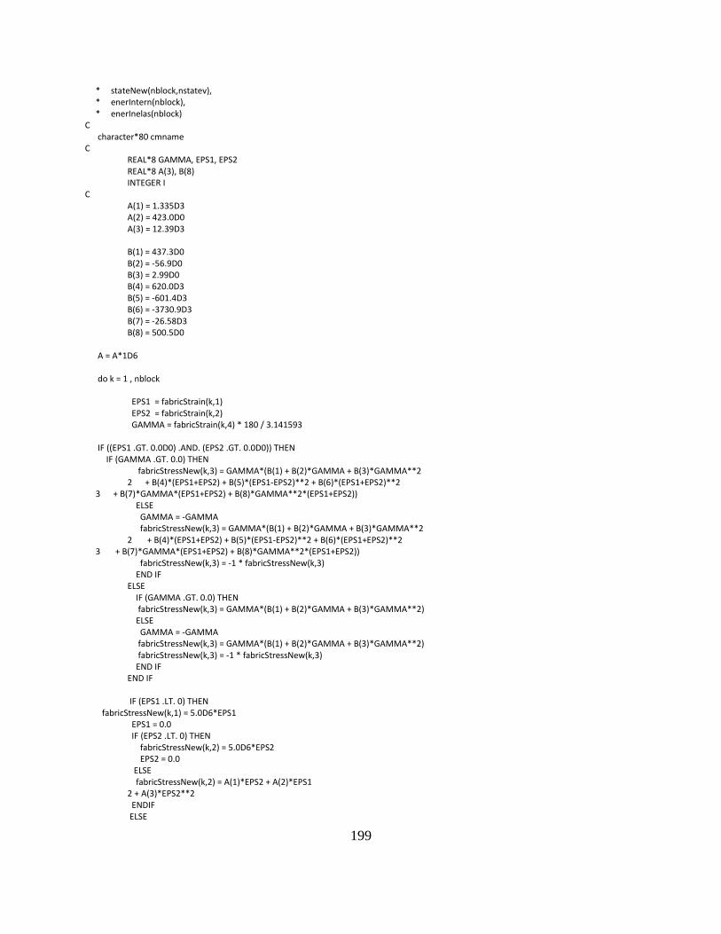
199
* stateNew(nblock,nstatev), * enerIntern(nblock), * enerInelas(nblock) C character*80 cmname C REAL*8 GAMMA, EPS1, EPS2 REAL*8 A(3), B(8) INTEGER I C A(1) = 1.335D3 A(2) = 423.0D0 A(3) = 12.39D3 B(1) = 437.3D0 B(2) = -56.9D0 B(3) = 2.99D0 B(4) = 620.0D3 B(5) = -601.4D3 B(6) = -3730.9D3 B(7) = -26.58D3 B(8) = 500.5D0 A = A*1D6 do k = 1 , nblock EPS1 = fabricStrain(k,1) EPS2 = fabricStrain(k,2) GAMMA = fabricStrain(k,4) * 180 / 3.141593 IF ((EPS1 .GT. 0.0D0) .AND. (EPS2 .GT. 0.0D0)) THEN IF (GAMMA .GT. 0.0) THEN fabricStressNew(k,3) = GAMMA*(B(1) + B(2)*GAMMA + B(3)*GAMMA**2 2 + B(4)*(EPS1+EPS2) + B(5)*(EPS1-EPS2)**2 + B(6)*(EPS1+EPS2)**2 3 + B(7)*GAMMA*(EPS1+EPS2) + B(8)*GAMMA**2*(EPS1+EPS2)) ELSE GAMMA = -GAMMA fabricStressNew(k,3) = GAMMA*(B(1) + B(2)*GAMMA + B(3)*GAMMA**2 2 + B(4)*(EPS1+EPS2) + B(5)*(EPS1-EPS2)**2 + B(6)*(EPS1+EPS2)**2 3 + B(7)*GAMMA*(EPS1+EPS2) + B(8)*GAMMA**2*(EPS1+EPS2)) fabricStressNew(k,3) = -1 * fabricStressNew(k,3) END IF ELSE IF (GAMMA .GT. 0.0) THEN fabricStressNew(k,3) = GAMMA*(B(1) + B(2)*GAMMA + B(3)*GAMMA**2) ELSE GAMMA = -GAMMA fabricStressNew(k,3) = GAMMA*(B(1) + B(2)*GAMMA + B(3)*GAMMA**2) fabricStressNew(k,3) = -1 * fabricStressNew(k,3) END IF END IF IF (EPS1 .LT. 0) THEN fabricStressNew(k,1) = 5.0D6*EPS1 EPS1 = 0.0 IF (EPS2 .LT. 0) THEN fabricStressNew(k,2) = 5.0D6*EPS2 EPS2 = 0.0 ELSE fabricStressNew(k,2) = A(1)*EPS2 + A(2)*EPS1 2 + A(3)*EPS2**2 ENDIF ELSE

200
IF (EPS2 .LT. 0) THEN fabricStressNew(k,2) = 5.0D6*EPS2 EPS2 = 0.0 fabricStressNew(k,1) = A(1)*EPS1 + A(2)*EPS2 2 + A(3)*EPS1**2 ELSE fabricStressNew(k,1) = A(1)*EPS1 + A(2)*EPS2 2 + A(3)*EPS1**2 fabricStressNew(k,2) = A(1)*EPS2 + A(2)*EPS1 2 + A(3)*EPS2**2 ENDIF ENDIF end do return end