Embed Size (px)
Citation preview
Multiple hurdle models in R The mhurdle Package
Fabrizio CarlevaroUniversite de Geneve
Yves CroissantUniversite de la Reunion
Stephane HoareauUniversite de la Reunion
Abstract
mhurdle is a package for R enabling the estimation of a wide set of models for which theresponse is zero left-censored This kind of models are called limited dependent or Tobitmodels in the econometric literature and are of particular interest to analyze householdsrsquoconsumption data provided by family expenditure surveys
Keywords˜limited dependent variable maximum likelihood estimation R
1 Introduction
In applied econometric studies the dependent variable often exhibits a large proportion offixed values eg
bull the number of hours of work supplied is zero for all unemployed or inactive persons
bull the expenditure for particular goods are nil for all households not consuming thesegoods
bull the attendance of a show is always equal to the capacity of the room each time the showis performed at ldquoposition closedrdquo
In these circumstances ordinary least-squares estimation is biased and inconsistent Howeverthe model can be estimated consistently using maximum likelihood methods by taking intoaccount the censored nature of the dependent variable
This problem has been treated for a long time in the statistics literature dealing with survivalmodels which are implemented in R with the survival package of Therneau and Lumley (2008)
It has also close links with the problem of selection bias for which some methods are imple-mented in the sampleSelection package of Toomet and Henningsen (2008b)
mhurdle deals specifically with models where the dependent variable is zero-left censoredand the observationsrsquo sample consequently may present a large proportion of zeros which istypically the case in household expenditure surveys1
1This package has been developed as part of a PhD dissertation carried out by Stephane Hoareau (2009)at the University of La Reunion under the supervision of Fabrizio Carlevaro and Yves Croissant
2 Multiple hurdle models in R The mhurdle Package
Since Tobin (1958) seminal paper a large econometric literature has been developed to dealcorrectly with this problem of zero observations More specifically zero observations mayappear for the following three reasons
lack of resources the household would like to consume the good but cannot afford it withits present budget
good rejection the good is not selected by the household because it is harmful or can bereplaced by some substitute good
purchase infrequency the good is bought by the household but with a low frequencyso that zero expenditure may be observed if the survey is carried out over a too shortperiod (see Deaton and Irish 1984)
The original Tobinrsquos model takes only the first source of zeros into account With mhurdlethe three sources of zero may be introduced in the model
For each of the three sources of zeros a continuous latent variable is defined with a zeroobserved if the latent variable is negative These latent variables are defined as the sumof a linear combination of covariates and a random disturbance with a possible correlationbetween the disturbances of different latent variables
The paper is organized as follows Section˜2 presents an overview of the theoretical modelsused Section˜3 presents the theoretical framework for model estimation evaluation andselection Section˜4 discusses the software rationale used in the package Section˜5 illustratesthe use of mhurdle with several examples Section˜6 concludes
2 Econometric framework
21 Model specification
Our modeling strategy rests on the following three equationsylowast1 = βgt1 x1 + ε1ylowast2 = βgt2 x2 + ε2ylowast3 = βgt3 x3 + ε3
where x1 x2 x3 stand for column-vectors of explanatory variables (called covariates in thefollowings) β1 β2 β3 for column-vectors of the impact coefficients of the explanatory variableson the dependent variables ylowast1 ylowast2 ylowast3 and ε1 ε2 ε3 for random disturbances
bull The first equation defines the good selection mechanism if ylowast1 lt 0 the good is notconsumed because it is not identified by the household as a relevant consumption good
bull The second equation defines the desired consumption level of the good therefore ifylowast2 lt 0 the good is not consumed as a negative consumption level implied by the budgetconstraint cannot be realized
Fabrizio Carlevaro Yves Croissant Stephane Hoareau 3
bull The third equation defines the frequency of purchase mechanism if ylowast3 lt 0 the good isnot purchased during the survey period while it is purchased at least one time whenylowast3 gt 0 Assuming that the survey period is a fraction P of the purchase period apurchase y = ylowast2P is observed with probability P = Probylowast3 gt 0 during the surveywhile no purchase is observed with probability (1minus P )
As ylowast1 and ylowast3 are unobservable indicators of dichotomous variables ε1 and ε3 stand for N(0 1)random disturbances while ε2 sim N(0 σ2) with unknown σ2 since ylowast2 is an observable variablewhen uncensored
A priori information may suggest that one or more of these censoring mechanisms is ineffectiveFor instance we know in advance that all households purchase food regularly implying thatthe first two censoring mechanisms are inoperative for food In this case the relevant modelis defined by only two equations one defining the desired consumption level of food andthe other the decision of food purchasing during the survey period Besides the desiredconsumption equation explaining dependent variable ylowast2 must be specified as a non negativeparametric function of covariates x2 and random disturbance ε2 For the time being twofunctional forms of this equation have been programmed in mhurdle namely a log-normalfunctional form
ln ylowast2 = βgt2 x2 + ε2
and a truncated normal functional form defined by a linear desired consumption equationwith ε2 distributed according to a N(0 σ2) left-truncated at ε2 = minusβgt2 x2 as suggested byCragg (1971)
A priori information may also suggest to set to zero some or all correlations between randomdisturbances ε1 ε2 ε3 entailing a partial or total independence between the above definedcensoring mechanisms In particular it seems appropriate to a priori suppose zero correlationbetween ε1 and ε3 as well as between ε2 and ε3 as a consequence of the different nature in thedeterminants responsible on one hand of the good selection and desired consumption leveldecisions and on the other hand of those responsible of the frequency of purchase decision
Figure 1 outlines the full set of special models that can be generated from this general econo-metric framework by enforcing ineffective censoring mechanisms and by selecting an appro-priate functional form of the desired consumption equation
This figure shows that 12 different consistent models can be estimated by the mhurdle packageleading to 23 different parametric specifications when no correlation between random distur-bances ε1 and ε2 is considered as a different specification assumption from that of correlateddisturbances
Note that among these models two are not concerned by censored data namely models 1and 2 These two specifications are relevant only for modeling uncensored samples
All the other models are potentially able to analyze censored samples by combining up tothe three censoring mechanisms described above With the notable exception of the standardTobit model that can be estimated also by the survival package of Therneau and Lumley(2008) these models cannot be found in an other R-library
Some of mhurdle models have already been used in the applied econometric literature Inparticular models 3 and 4 are single hurdle good selection models originated by Cragg (1971)
4 Multiple hurdle models in R The mhurdle Package
Lack
of
ress
ou
rces
(eq
uat
ion
2)
Fun
ctio
nal
form
of
des
ired
con
sum
pti
on
Go
od
reje
ctio
n
(eq
uat
ion
1)
TRU
E
FALS
E
TRU
E
FALS
E
FALS
E
TRU
E
FALS
E
n
n n
n
l
Mo
del
12
(Tri
ple
Hu
rdle
mo
del
)
Mo
del
8 (
Do
ub
le H
urd
le m
od
el)
Mo
del
11
(P-T
ob
it m
od
el)
Mo
del
5 (
Tob
it m
od
el)
Mo
del
9
Mo
del
10
Mo
del
1
Mo
del
4
Mo
del
6
Mo
del
7
Mo
del
3
Mo
del
2 M
od
els
t l t l t l t
Lack
of
ress
ou
rces
(eq
uat
ion
2)
Pu
rch
ase
infr
equ
ency
(eq
uat
ion
3)
Fun
ctio
nal
form
of
des
ired
con
sum
pti
on
TRU
E
TRU
E
TRU
E
FALS
E
FALS
E
FALS
E
TRU
E
n=n
orm
al
l=lo
g-n
orm
al
t=tr
un
cate
d-n
orm
al
Figure 1 The full set of mhurdle special models
The double hurdle model combining uncorrelated good selection and lack of resources cen-
Fabrizio Carlevaro Yves Croissant Stephane Hoareau 5
soring mechanisms is also due to Cragg (1971) the correlated version of this double hurdlemodel has been originated by Blundell and Meghir (1987)
P-Tobit model is due to Deaton and Irish (1984) and explains zero purchases as the resultof lack of resources andor infrequent purchases Models 6 and 7 are single hurdle modelsnot yet used in applied demand analysis where the operating censoring mechanism is due toinfrequent purchases
Among the original models encompassed by mhurdle models 9 and 10 are double hurdlemodels combining good selection and frequency of purchase mechanisms to explain censoredsamples
Model 12 is an original three hurdle model originated in Hoareau (2009) This model ex-plains censored purchases either as the result of good rejection lack of resources or infrequentpurchases
22 Likelihood function
As for the standard Tobit model the likelihood of our censored models have two componentsthe first one is the probability of a binary choice (purchasing or not) the second one isthe density function of the chosen expenditure level of consumption for the households thatconsume
The contribution of a zero observation to the sample log-likelihood function can be writtenas follow
lnLminusi =
ln(
1minus Φ(βgt1 x1i
βgt2 x2iσ ρ
)Φ(βgt3 x3i)
)for normal models
ln(1minus Φ(βgt1 x1i)Φ(βgt3 x3i)
)for log-normal models
ln
1minusΦ
(βgt1 x1i
βgt2 x2iσ
ρ
)Φ
(βgt2 x2iσ
) Φ(βgt3 x3i)
for truncated-normal models
where Φ(z) denotes the distribution function of a N(0 1) random variable We remind thatlog-normal and truncated normal models assume that the lack of resources mechanism isinoperative whereas it is operative in normal models
The second and the third expression correspond to the case where a zero purchase is observedonly for good rejection or for purchase infrequency reasons In the second expression thedesired consumption equation is specified according to a log-normal functional form whereasin the third expression it is specified according to a truncated-normal functional form Thefirst expression corresponds to the case where a zero purchase is observed either for goodrejection for lack of resources or for purchase infrequency reasons
These expressions become simpler in the following special cases
bull when the good selection mechanism is inoperative implying
Pylowast1i gt 0 = Φ(βgt1 x1i) = 1
and consequently
lnLminusi =
ln(
1minus Φ(βgt2 x2iσ
)Φ(βgt3 x3i)
)for normal models
ln(1minus Φ(βgt3 x3i)
)otherwise
6 Multiple hurdle models in R The mhurdle Package
bull when the purchase frequency mechanism is inoperative implying
Pylowast3i gt 0 = Φ(βgt3 x3i) = 1
and consequently
lnLminusi =
ln(
1minus Φ(βgt1 x1i
βgt2 x2iσ ρ
))for normal models
ln(1minus Φ(βgt1 x1i)
)for log-normal models
ln
1minusΦ
(βgt1 x1i
βgt2 x2iσ
ρ
)Φ
(βgt2 x2iσ
) for truncated-normal models
bull when the good selection mechanism and the desired consumption equation are uncorre-lated (ρ = 0) implying
Φ
(βgt1 x1i
βgt2 x2i
σ 0
)= Φ(βgt1 x1i)Φ
(βgt2 x2i
σ
)and consequently
lnLminusi =
ln(
1minus Φ(βgt1 x1i)Φ(βgt2 x2iσ
)Φ(βgt3 x3i)
)for normal models
ln(1minus Φ(βgt1 x1i)Φ(βgt3 x3i)
)otherwise
bull when both the good selection and the frequency of purchase mechanisms are inoperativeimplying
lnLminusi =
ln(
1minus Φ(βgt2 x2iσ
))for normal models
minusinfin for log-normal and truncated-normal models
Consequently in this very special case log-normal and truncated-normal model speci-fications can only be used to analyze uncensored samples
The contribution of a positive observation to the log-likelihood function is best presented bydefining a ldquoresidualrdquo of the fit as
ei =
ln yi + ln Φ(βgt3 x3i)minus βgt2 x2i for log-normal modelsyiΦ(βgt3 x3i)minus βgt2 x2i otherwise
One observes that the parameters and the covariates of the frequency of purchase equationenter the definition of this ldquoresidualrdquo because this residual is defined for the average consump-tion which depends on the probability of purchasing as described previously
The contribution of a positive observation to the log-likelihood function is then written as
lnL+i = minus lnσ + lnφ
(eiσ
)+ ln Φ
(βgt1 x1i+
ρσeiradic
(1minusρ2)
)+ ln Φ(βgt3 x3i)
+
ln Φ(βgt3 x3i) for normal modelsminus ln yi for log-normal models
minus ln Φ(βgt2 x2iσ
)+ ln Φ(βgt3 x3i) for truncated-normal models
Fabrizio Carlevaro Yves Croissant Stephane Hoareau 7
where φ(z) denotes the density function of a N(0 1) random variable
As for the log-likelihood function of a censored observation the expression of the log-likelihoodfunction of an uncensored observation become simpler in the following special cases
bull when the good selection mechanism is inoperative implying
lnL+i = minus lnσ + lnφ
(eiσ
)+ ln Φ(βgt3 x3i)
+
ln Φ(βgt3 x3i ) for normal modelsminus ln yi for log-normal models
minus ln Φ(βgt2 x2iσ
)+ ln Φ(βgt3 x3i ) for truncated-normal models
bull when the purchase frequency mechanism is inoperative implying
ei =
ln yi minus βgt2 x2i for log-normal modelsyi minus βgt2 x2i otherwise
and
lnL+i = minus lnσ + lnφ
(eiσ
)+ ln Φ
(βgt1 x1i+
ρσeiradic
(1minusρ2)
)+
minus ln yi for log-normal models
minus ln Φ(βgt2 x2iσ
)for truncated-normal models
bull when the good selection mechanism and the desired consumption equation are uncorre-lated (ρ = 0) implying
lnL+i = minus lnσ + lnφ
(eiσ
)+ ln Φ(βgt1 x1i) + ln Φ(βgt3 x3i)
+
ln Φ(βgt3 x3i ) for normal modelsminus ln yi for log-normal models
minus ln Φ(βgt2 x2iσ
)+ ln Φ(βgt3 x3i ) for truncated-normal models
bull when both the good selection and the frequency of purchase mechanisms are inoperativeimplying
ei =
ln yi minus βgt2 x2i for log-normal modelsyi minus βgt2 x2i otherwise
and
lnL+i = minus lnσ + lnφ
(eiσ
)+
minus ln yi for log-normal models
minus ln Φ(βgt2 x2iσ
)for truncated-normal models
8 Multiple hurdle models in R The mhurdle Package
Combining these log-likelihood function for zero and positive expenditure observations thesample log-likelihood function is written as
lnL =sumi|yi=0
lnLminusi +sumi|yigt0
lnL+i
Note that for uncorrelated single-hurdle good selection models lnLminusi depends only on β1 andlnL+
i depends only on β2 and σ allowing to separate the model estimation according to twoindependent models
bull a binary probit model allowing to estimate β1 independently of β2 and σ
bull a linear log-linear or truncated regression model allowing to estimate β2 and σ inde-pendently of β1
3 Model estimation evaluation and selection
The econometric framework described in the previous section provides a theoretical frameworkfor tackling the problems of model estimation evaluation and selection within the statisticaltheory of classical inference
31 Model estimation
The full parametric specification of our multiple hurdle models allows to efficiently estimatetheir parameters by means of the maximum likelihood principle Indeed it is well knownfrom classical estimation theory that under the assumption of correct model specificationand for a likelihood function sufficiently well behaved the maximum likelihood estimator isasymptotically efficient within the class of consistent and asymptotically normal estimators2
More precisely the asymptotic distribution of the maximum likelihood estimator θ of a mhur-dle model parameter vector θ is written as
θAsim N(θ
1
nIA(θ)minus1)
whereAsim stands for rdquoasymptotically distributed asrdquo and
IA(θ) = plim1
n
nsumi=1
E(part2 lnLi(θ)
partθpartθgt) = plim
1
n
nsumi=1
E(part lnLi(θ)
partθ
part lnLi(θ)
partθgt)
for the asymptotic RA Fisher information matrix of a sample of n independent observations
More generally any inference about a differentiable vector function of θ denoted by γ = h(θ)can be based on the asymptotic distribution of its implied maximum likelihood estimatorγ = h(θ) This distribution can be derived from the asymptotic distribution of θ accordingto the so called delta method
2See Amemiya (1985) chapter 4 for a more rigorous statement of this property
Fabrizio Carlevaro Yves Croissant Stephane Hoareau 9
γAsim h(θ) +
parth
partθgt(θ minus θ) Asim N(γ
1
n
parth
partθgtIA(θ)minus1parth
gt
partθ)
The practical use of these asymptotic distributions requires to replace the theoretical variance-covariance matrix of these asymptotic distributions with consistent estimators which can be
obtained by using parth(θ)partθgt
as a consistent estimator for parth(θ)partθgt
and either 1n
sumni=1
part2 lnLi(θ)partθpartθgt
or
1n
sumni=1
part lnLi(θ)partθ
part lnLi(θ)partθgt
as a consistent estimator for IA(θ) The last two estimators are di-rectly provided by two standard iterative methods used to compute the maximum likelihoodparameterrsquos estimate namely the Newton-Raphson method and the Berndt Hall Hall Haus-man or BHHH method respectively mentioned in section 43
32 Model evaluation
Two fundamental principles should be used to appraise the results of a model estimationnamely its economic relevance and its statistical and predictive adequacy The first principledeals with the issues of accordance of model estimate with the economic rationale underlyingthe model specification and of its relevance for answering the questions for which the modelhas been built These issues are essentially context specific and therefore cannot be dealtwith generic criteria The second principle refers to the issues of empirical soundness of modelestimate and of its ability to predict sample or out-of-sample observations These issues can betackled by means of formal tests of significance based on the previously presented asymptoticdistributions of model estimates and by measures of goodness of fitprediction respectively
To assess the goodness of fit of mhurdle estimates two pseudo R2 coefficients are providedThe first one is an extension of the classical coefficient of determination used to explain thefraction of variation of the dependent variable explained by the covariates included in a linearregression model with intercept The second one is an extension of the likelihood ratio indexintroduced McFadden (1974) to measure the relative gain in the maximized log-likelihoodfunction due to the covariates included in a qualitative response model
To define a pseudo coefficient of determination we rely on the non linear regression modelexplaining the dependent variable of a mhurdle model This model is written as
yi = E(yi) + εi i = 1 n
where εi stands for a zero expectation heteroskedastic random disturbance and E(yi) =Probyi gt 0E(yi|yi gt 0) with Probyi gt 0 = 1minus Lminusi and
E(yi|yi gt 0) =
βgt2 x2i
Φ(βgt3 x3i)+ σ
ψn(βgt1 x1iβgt2 x2iσ
ρ)
Φ(βgt1 x1iβgt2 x2iσ
ρ)Φ(βgt3 x3i)for normal and truncated-normal models
expβgt2 x2i+05σ2(1minusρ2)ψl(βgt1 x1iρσ)
Φ(βgt1 x1i)Φ(βgt3 x3i)for log-normal models
where
ψn(βgt1 x1iβgt2 x2i
σ ρ) =
int infinminusβgt1 x1i
[ρε1Φ
(βgt2 x2iσ + ρε1radic
1minus ρ2
)+radic
1minus ρ2φ
(βgt2 x2iσ + ρε1radic
1minus ρ2
)]φ(ε1)dε1
10 Multiple hurdle models in R The mhurdle Package
and
ψl(βgt1 x1i ρσ) =
int infinminusβgt1 x1i
expρσε1φ(ε1)dε1
Notice that these two last integrals can be computed using the first terms of a Taylor seriesexpansion around ρ = 0 and ρσ = 0 respectively as detailed for the first integral in CarlevaroCroissant and Hoareau (2008) Moreover the above general expressions of E(yi|yi gt 0)become simpler in the following special cases
bull when the good selection mechanism is inoperative (Φ(βgt1 x1i) = 1) leading to
E(yi|yi gt 0) =
βgt2 x2i
Φ(βgt3 x3i)+ σ
φ(βgt2 x2iσ
Φ(βgt2 x2iσ
)Φ(βgt3 x3i)for normal and truncated-normal models
expβgt2 x2i+05σ2Φ(βgt3 x3i)
for log-normal models
bull when the purchase frequency mechanism is inoperative (Φ(βgt3 x3i) = 1) leading to
E(yi|yi gt 0) =
βgt2 x2i + σ
ψn(βgt1 x1iβgt2 x2iσ
ρ)
Φ(βgt1 x1iβgt2 x2iσ
ρ)for normal and truncated-normal models
expβgt2 x2i + 05σ2
(1minus ρ2
) ψl(βgt1 x1iρσ)
Φ(βgt1 x1i)for log-normal models
bull when the good selection mechanism and the desired consumption equation are uncorre-lated (ρ = 0) implying
Φ
(βgt1 x1i
βgt2 x2i
σ 0
)= Φ(βgt1 x1i)Φ
(βgt2 x2i
σ
)as well as
ψn
(βgt1 x1i
βgt2 x2i
σ 0
)= ψl
(βgt1 x1i 0
)= Φ(βgt1 x1i)
and consequently
E(yi|yi gt 0) =
βgt2 x2i
Φ(βgt3 x3i)+ σ
φ
(βgt2 x2iσ
)Φ(
βgt2 x2iσ
)Φ(βgt3 x3i)for normal and truncated-normal models
expβgt2 x2i+05σ2Φ(βgt3 x3i)
for log-normal models
namely the same formulas of E(yi|yi gt 0) as when the good selection mechanism isinoperative
Fabrizio Carlevaro Yves Croissant Stephane Hoareau 11
bull when both the good selection and the frequency of purchase mechanisms are inoperativeleading to
E(yi|yi gt 0) =
βgt2 x2i + σφ
(βgt2 x2iσ
)Φ(
βgt2 x2iσ
)for normal and truncated-normal models
expβgt2 x2i + 05σ2
for log-normal models
Denoting by yi the fitted values of yi obtained by computing predictor E(yi) for yi withthe maximum likelihood estimate of model parameters we define a pseudo coefficient ofdetermination for a mhurdle model according to the following formula
R2 = 1minus RSS
TSS
with RSS =sum
(yi minus yi)2 the residual sum of squares and TSS =sum
(yi minus y0)2 the total sumof squares where y0 denotes the maximum likelihood estimate of E(yi) in the mhurdle modelwithout covariates (intercept-only model) Notice that this goodness of fit measure cannotexceed one but can be negative as a consequence of the non linearity of E(yi) with respectto the parameters
Two other formulas which are equivalent to compute R2 in the linear regression model withintercept could have been used to define a pseudo coefficient of determination namely theratio of the explained sum of square to the total sum of squares or the squared correlationbetween actual and fitted values We disregarded these alternatives because the former mea-sure can exceed one in a non linear regression model while the latter although providingvalues always within zero and one cannot be adjusted for degrees of freedom for a use as amodel selection criterion A more promising approach consists in computing RSS and TSSwith standardized residuals to correct for the heteroskedasticity of row residuals This Pear-son goodness of fit measure requiring to write down analytically the variance of εi is notcurrently implemented
The extension of the McFadden likelihood ratio index for qualitative response models tomhurdle models is straightforwardly obtained by substituting in this index formula
ρ2 = 1minus lnL(θ)
lnL(α)=
lnL(α)minus lnL(θ)
lnL(α)
the maximized log-likelihood function of a qualitative response model with covariates and thelog-likelihood function of the corresponding model without covariates or intercept-only modelwith the maximized log-likelihood functions of a mhurdle model with covariates lnL(θ) andwithout covariates lnL(α) respectively This goodness of fit measure takes values within zeroand one and as it can be easily inferred from the above second expression of ρ2 it measuresthe relative increase of the maximized log-likelihood function due to the use of explanatoryvariables with respect to the maximized log-likelihood function of a naive intercept-only model
33 Model selection
Model selection deals with the problem of discriminating between alternative model specifi-cations used to explain the same dependent variable with the view of finding the one best
12 Multiple hurdle models in R The mhurdle Package
suited to explain the sample of observations at hand This decision problem can be tackledfrom two point of view namely that of the model specification achieving the best in-samplefit on one hand and that of the model specification that is favored in a formal test comparingtwo model alternatives on the other hand
The first selection criterion is easy to apply as it consists in comparing one of the above definedmeasures of fit computed for the competing model specifications after adjusting them for theloss of sample degrees of freedom due to model parametrization Indeed the value of thesemeasures of fit can be improved by increasing model parametrization in particular when theparameter estimates are obtained by optimizing a criteria functionally related to the selectedmeasure of fit as it is the case when using the ρ2 fit measure with a maximum likelihoodestimate Consequently a penalty that increases with the number of model parameters shouldbe added to the R2 and ρ2 fit measures to trade off goodness of fit improvements withparameter parsimony losses
To define an adjusted pseudo coefficient of determination we rely on Theil (1971)rsquos correctionof R2 in a linear regression model defined by
R2 = 1minus nminusK0
nminusKRSS
TSS
where K and K0 stand for the number of parameters of the mhurdle model with covariatesand without covariates respectively Therefore choosing the model specification with thelargest R2 is equivalent to choosing the model specification with the smallest model residualvariance estimate s2 = RSS
nminusK
To define an adjusted likelihood ratio index we replace in this goodness of fit measure ρ2
the log-likelihood criterion with the Akaike information criterion AIC = minus2 lnL(θ) + 2KTherefore choosing the model specification with the largest
ρ2 = 1minus lnL(θ)minusKlnL(α)minusK0
is equivalent to choosing the model specification that minimizes the Akaike (1973) predictorof the Kullback-Liebler Information Criterion (KLIC) This criterion measures the distancebetween the conditional density function f(y|x θ) of a possibly misspecified parametric modeland that of the true unknown model denoted by h(y|x) It is defined by the following formula
KLIC = E
[ln
(h(y|x)
f(y|x θlowast)
)]=
intln
(h(y|x)
f(y|x θlowast)
)dH(y x)
where H(y x) denotes the distribution function of the true joint distribution of (y x) and θlowastthe probability limit with respect to H(y x) of θ the so called quasi-maximum likelihoodestimator obtained by applying the maximum likelihood when f(y|x θ) is misspecified
Our second model selection criterion relies on the use of a test proposed by Vuong (1989)According to the rationale of this test the rdquobestrdquo parametric model specification among acollection of competing specifications is the one that minimizes the KLIC criterion or equiv-alently the specification for which the quantity
E[ln f(y|x θlowast)] =
intln f(y|x θlowast)dH(y x)
Fabrizio Carlevaro Yves Croissant Stephane Hoareau 13
is the largest Therefore given two competing conditional models with density functionsf(y|x θ) and g(y|xπ) and parameter vectors θ and π of size K and L respectively Vuongsuggests to discriminate between these models by testing the null hypothesis
H0 E[ln f(y|x θlowast)] = E[ln g(y|xπlowast)]lArrrArr E
[lnf(y|x θlowast)
g(y|xπlowast)
]= 0
meaning that the two models are equivalent against
Hf E[ln f(y|x θlowast)] gt E[ln g(y|xπlowast)]lArrrArr E
[lnf(y|x θlowast)
g(y|xπlowast)
]gt 0
meaning that specification f(y|x θ) is better than g(y|xπ) or against
Hg E[ln f(y|x θlowast)] lt E[ln g(y|x θlowast)]lArrrArr E
[lnf(y|x θlowast)
g(y|xπlowast)
]lt 0
meaning that specification g(y|xπ) is better than f(y|x θ)
The quantity E[ln f(y|x θlowast)] is unknown but it can be consistently estimated under some reg-ularity conditions by 1n times the log-likelihood evaluated at the quasi-maximum likelihoodestimator Hence 1n times the log-likelihood ratio (LR) statistic
LR(θ π) =nsumi=1
lnf(yi|xi θ)g(yi|xi π)
is a consistent estimator of E[ln f(y|xθlowast)
g(y|xπlowast)
] Therefore an obvious test of H0 consists in
verifying whether the LR statistic differs from zero The distribution of this statistic can bework out even when the true model is unknown as the quasi-maximum likelihood estimatorsθ and π converge in probability to the pseudo-true values θlowast and πlowast respectively and haveasymptotic normal distributions centered on these pseudo-true values
The resulting distribution of LR(θ π) depends on the relation linking the two competing mod-els To this purpose Vuong differentiates among three types of competing models namelynested strictly non nested and overlapping However for model comparisons within the setof mhurdle special models presented in FIG 1 only the first two cases are really relevant atleast as long as we compare model specifications with identical covariates
A parametric model Gπ defined by the conditional density function (cdf) g(y|xπ) is saidto be nested in parametric model Fθ with cdf f(y|x θ) if and only if any cdf of Gπ isequal to a cdf of Fθ for almost all x Within our mhurdle special models this is the casewhen comparing two specifications differing only with respect to the presence or the absenceof correlated disturbances For these models it is necessarily the case that f(y|x θlowast) equivg(y|xπlowast) Therefore H0 is tested against Hf
If model Fθ is misspecified it has been shown by Vuong that
bull under H0 the quantity 2LR(θ π) converges in distribution towards a weighted sum ofK + L iid χ2(1) random variables where the weights are the K + L possibly negativeeigenvalues of a theoretical symmetric matrix that can be consistently estimated by a
14 Multiple hurdle models in R The mhurdle Package
sample analogue Notice that the density function of this random variable has not beenworked out analytically Therefore we compute it by simulation
bull under Hf the same statistic converge almost surely towards +infin
As a consequence for a test with critical value c H0 is rejected in favor of Hf if 2LR(θ π) gt c
or if the p-value associated to the observed value of 2LR(θ π) is less than the significancelevel of the test Notice that if model Fθ is correctly specified the asymptotic distributionof the LR statistic is as expected a χ2 random variable with K minus L degrees of freedom
Two parametric models Fθ and Gπ defined by cdf f(y|x θ) and g(y|xπ) are said to bestrictly non-nested if and only if no cdf of model Fθ is equal to a cdf of Gπ for almostall x and conversely Within mhurdle special models this is the case when comparing twospecifications differing with respect either to the effective censoring mechanisms or to thefunctional form of the desired consumption equation For these models it is necessarily thecase that f(y|x θlowast) 6= g(y|xπlowast) implying that both models are misspecified under H0
For such strictly non-nested models Vuong has shown that
bull under H0 the quantity nminus12LR(θ π) converges in distribution towards a normal ran-dom variable with zero expectation and variance
ω2 = V
(lnf(y|x θlowast)
g(y|xπlowast)
)computed with respect to the distribution function of the true joint distribution of (y x)
bull under Hf the same statistic converge almost surely towards +infin
bull under Hg the same statistic converge almost surely towards minusinfin
Hence H0 is tested against Hf or Hg using the standardized LR statistic
TLR =LR(θ π)radic
nω
where ω2 denotes the following consistent estimator for ω2
ω2 =1
n
nsumi=1
(lnf(yi|xi θ)g(yi|xi π)
)2
minus
(1
n
nsumi=1
lnf(yi|xi θ)g(yi|xi π)
)2
As a consequence for a test with critical value c H0 is rejected in favor of Hf if TLR gt cor if the p-value associated to the observed value of TLR in less than the significance level ofthe test Conversely H0 is rejected in favor of Hg if TLR lt minusc or if the p-value associated tothe observed value of |TLR| in less than the significance level of the test Notice that if oneof models Fθ or Gπ is assumed to be correctly specified the Cox (1961 1962) LR test of nonnested models needs to be used
4 Software rationale
Fabrizio Carlevaro Yves Croissant Stephane Hoareau 15
There are three important issues to be addressed to correctly implement in R the econometricframework described in the previous section The first one is to provide a good interface todescribe the model to be estimated The second one is the problem of finding good startingvalues for computing model estimates The third one is to offer flexible optimization tools forlikelihood maximization
41 Model syntax
In R the model to be estimated is described using formula objects the left-hand side denotingthe censored dependent variable y and the right-hand side the functional relation explainingy as a function of covariates For example y ~ x1 + x2x3 indicates that y linearly dependson variables x1x2x3 and on the interaction term x2 times x3
For the models implemented in mhurdle three kinds of covariates should be specified theones of the consumption equation (denoted x2) the ones of the selection equation (denotedx1) and those of the infrequency equation (denoted x3) To define a model with three kindsof covariates a general solution is given by the Formula package developed by Zeileis andCroissant (2010) which provides extended formula objects To define a model where y isthe censored dependent variable x21 and x22 two covariates for the desired consumptionequation x11 and x12 two covariates for the selection and x31 and x32 two covariates for theinfrequency of purchase equation we use the following commands
Rgt library(Formula)
Rgt f lt- Formula(y ~ x11 + x12 | x21 + x22 | x31 + x32)
To illustrate the use of Formula letrsquos use the tobin dataframe from the survival packageThis dataframe is a sub-sample of 20 observations of the original data used by Tobin (1958)in his seminal paper
Rgt data(tobin package = survival)
Rgt head(tobin 3)
durable age quant
1 00 577 236
2 07 509 283
3 00 485 207
The variables of this dataframe are
durable the durable good expenditures in thousands of US$
age the age of the head of the family in years
quant the liquidity ratio in per thousands
To estimate a model for durable good expenditures using age and quant as covariates forthe desired consumption equation age for the selection equation and quant for the purchaseinfrequency equation we use the following syntax
16 Multiple hurdle models in R The mhurdle Package
Rgt f lt- Formula(durable ~ age | age + quant | quant)
Several methods are provided to deal with these extended formulas In particular the modelcovariate matrices for the three equations are easily computed using
Rgt S lt- modelmatrix(f data = tobin rhs = 1)
Rgt X lt- modelmatrix(f data = tobin rhs = 2)
Rgt P lt- modelmatrix(f data = tobin rhs = 3)
Rgt head(X 3)
(Intercept) age quant
1 1 577 236
2 1 509 283
3 1 485 207
Rgt head(S 3)
(Intercept) age
1 1 577
2 1 509
3 1 485
Rgt head(P 3)
(Intercept) quant
1 1 236
2 1 283
3 1 207
For the end user all these manipulations are internal to mhurdle function All he should do isentering a formula of the type y ~ x11 + x12 | x21 + x22 | x31 + x32 as first argumentof the function
42 Starting values
For the models we consider the log-likelihood function will be in general not concave More-over this kind of models are highly non linear with respect to parameters and thereforedifficult to estimate For these reasons the question of finding good starting values for theiterative computation of parameter estimates is crucial
As a less computer intensive alternative to maximum likelihood estimation Heckman (1976)has suggested a two step estimation procedure based on a respecification of the censoredvariable linear regression model sometimes called ldquoHeckitrdquo model avoiding inconsistency ofordinary least-squares estimator This two step estimator is consistent but inefficient It isimplemented in package sampleSelection
According to Carlevaro et˜al (2008) experience in applying this estimation procedure to two-hurdle models this approach doesnrsquot seem to work well with our correlated hurdle-models
Fabrizio Carlevaro Yves Croissant Stephane Hoareau 17
Indeed except for the very special case of model 3 (log-normal correlated single-hurdle selec-tion model) the probability of observing a censored purchase is not that of a simple probitmodel (see the formula of lnLminusi )
As noted previously for uncorrelated single-hurdle good selection models the estimationmay be performed in a sequence of two simple estimations namely the maximum likelihoodestimation of a standard dichotomous probit model followed by the ordinary least-squaresestimation of a linear log-linear or linear-truncated regression model In the last case packagetruncreg (Croissant 2009) is used
In case of correlated single-hurdle good selection models the coefficient maximum likelihoodestimate of the corresponding uncorrelated model (ρ = 0) is used as starting values
For purchase infrequency models (P-Tobit models) the starting values are computed usingan Heckman-like two step procedure In the first step parameters β3 are estimated using asimple probit In the second step a linear log-linear or linear-truncated model is estimatedon the sub-sample of uncensored observations using yiΦ(β
prime3x3) or ln yi + ln Φ(β
prime3x3) (in the
case of a log-normal specification) as the dependent variable of the regression model estimatedby ordinary least squares
43 Optimisation
Two kinds of routines are currently used for maximum likelihood estimation The first onecan be called ldquoNewton-likerdquo methods With these routines at each iteration an estimationof the log-likelihood hessian matrix is computed using either the second derivatives of thecriterion function (Newton-Raphson method) or the outer product of the gradient (BerndtHall Hall Hausman or BHHH method) This approach is very powerful if the criterionfunction is well-behaved but it may perform poorly otherwise and fail after a few iterations
The second one called Broyden Fletcher Goldfarb Shanno or BFGS method updates ateach iteration an estimate of the log-likelihood hessian matrix It is often more robust andmay perform better in cases where the former doesnrsquot work
Two optimization functions are included in core R nlm which uses the Newton-Raphsonmethod and optim which uses the BFGS method (among others) The recently developedmaxLik package by Toomet and Henningsen (2008a) provides a unified framework With aunique interface all the previously described methods are available
The behavior of maxLik can be controlled by the user using mhurdle arguments like printlevel(from 0-silent to 2-verbal) iterlim (the maximum number of iterations) methods (themethod used one of nr bhhh or bfgs) that are passed to maxLik
5 Examples
The package is loaded using
Rgt library(mhurdle)
51 Estimation
The estimation is performed using the mhurdle function which has the following arguments
18 Multiple hurdle models in R The mhurdle Package
formula a formula describing the model to estimate It should have three parts on the right-hand side specifying in the first part the desired consumption equation covariates inthe second part the good selection equation covariates and in the third part thepurchase frequency equation covariates
data a dataframe containing the observations of the variables present in the formula
subset weights naaction these are arguments passed on to the modelframe function inorder to extract the data suitable for the model These arguments are present in the lm
function and most of the estimation functions
start the starting values If NULL the starting values are computed as described in theprevious section
dist this argument indicates the functional form of the desired consumption equation whichmay be either log-normal l (the default) normal n or truncated normal t
corr a logical argument indicating whether the disturbances of the selection equation andthe consumption equation are correlated or not The default is FALSE
further arguments that are passed to the optimization function maxLik
Different combinations of these arguments lead to a large variety of models Note that someof them are logically inconsistent and therefore irrelevant For example a model with no goodselection equation and corr = TRUE is logically inconsistent because only good selection anddesired consumption equations can be correlated
To illustrate the use of mhurdle package we first estimate an independent triple-hurdle modelwhich we call model12i
Rgt model12i lt- mhurdle(durable ~ age + quant | age + quant | age +
+ quant tobin dist = n method = bfgs)
In applied work the issue may be to select the relevant hurdles As an alternative to thepreviously estimated three hurdle model we can now estimate more a priori restricted modelswhere only one or two hurdles are relevant
To estimate a model where only lack of resources is relevant to explain censored durable goodexpenditures we use
Rgt model5 lt- mhurdle(durable ~ 0 | age + quant | 0 tobin dist = n
+ method = nr)
To estimate an independent log-normal single-hurdle good rejection model we use
Rgt model3i lt- mhurdle(durable ~ age + quant | age + quant | 0 tobin
+ dist = l)
To estimate a log-normal single-hurdle purchase infrequency model we use
Fabrizio Carlevaro Yves Croissant Stephane Hoareau 19
Rgt model6 lt- mhurdle(durable ~ 0 | age + quant | age + quant tobin
+ dist = l)
To estimate an independent model where censured durable good expenditures may be ex-plained by lack of resources or good rejection we use
Rgt model8i lt- mhurdle(durable ~ age + quant | age + quant | 0 tobin
+ dist = n)
We then update this model in order to estimate a dependent double-hurdle (lack of resourcesor good rejection) model
Rgt model8d lt- update(model8i corr = TRUE)
52 Methods
A summary method is provided for mhurdle objects
Rgt summary(model8i)
Call
mhurdle(formula = durable ~ age + quant | age + quant | 0 data = tobin
dist = n)
Frequency of 0 065
Newton-Raphson maximisation
gradient close to zero
5 iterations 0h0m0s
g(-H)^-1g = 612E-22
Coefficients
Estimate Std Error t-value Pr(gt|t|)
sel(Intercept) 1461792 3710805 03939 06936338
selage -0122834 0072312 -16987 00893830
selquant 0017997 0015802 11389 02547578
reg(Intercept) 12841869 5321390 24133 00158108
regage 0404577 0098441 41098 3959e-05
regquant -0113719 0019904 -57132 1108e-08
sigma 1434599 0397077 36129 00003028
---
Signif codes 0 0001 001 005 01 1
Log-Likelihood -22186 on 7 Df
rho score test z = 0016 (pvalue = 0494)
20 Multiple hurdle models in R The mhurdle Package
R^2
McFadden 025143
Regression 037556
This method displays the percentage of 0 in the sample the coefficient table several measuresof goodness of fit and for independent models a score test of correlation
coef vcov logLik predict methods are provided in order to extract part of the results
Coefficients and the estimated asymptotic variance matrix of maximum likelihood estimatorsare extracted using the usual coef and vcov functions mhurdle object methods have a secondargument indicating which subset has to be returned (the default is to return all)
Rgt coef(model12i reg)
(Intercept) age quant
0200499276 0013152493 -0002808693
Rgt coef(model12i sel)
(Intercept) age quant
964594522 027385000 -007744716
Rgt coef(model12i sigma)
sigma
07949458
Rgt coef(summary(model12i) ifr)
Estimate Std Error t-value Pr(gt|t|)
(Intercept) 20520340 69683632 0002944786 09976504
age -25905681 3701866 -0069980062 09442095
quant 05774693 1034643 0055813405 09554905
Rgt vcov(model12i reg)
(Intercept) age quant
(Intercept) 1386563162 -0113600675 -00350976222
age -011360067 0008281271 -00011242924
quant -003509762 -0001124292 00003623083
Log-likelihood may be obtained for the estimated model or for a ldquonaiverdquo model ie a modelwithout covariates Moreover the component of the likelihood for null and for positive ob-servations may be obtained separately
Rgt logLik(model12i)
Fabrizio Carlevaro Yves Croissant Stephane Hoareau 21
[1] -181697
Rgt logLik(model12i which = positive)
[1] -1347851
Rgt logLik(model12i naive = TRUE which = zero)
zero
-5600195
Fitted values are obtained using the fitted function The output is a matrix whose twocolumns are the estimated probability of censoring Probyi = 0 and the estimated expectedvalue of an uncensored dependent variable observation E(yi|yi gt 0)
Rgt head(fitted(model12i))
zero positive
[1] 10000000 1809788e+29
[2] 04795935 1703160e+00
[3] 09999849 2743720e+05
[4] 04478696 4027116e+00
[5] 04366752 4276167e+00
[6] 10000000 4486644e+174
A predict function is also provided which returns the same two columns for given values ofthe covariates
Rgt pr lt- predict(model12i newdata = dataframe(durable = c(0 1
+ 0) age = c(50 32 48) quant = c(206 232 245)))
Rgt head(pr)
zero positive
[1] 10000000 9074063e+17
[2] 06532498 8239173e-01
[3] 04428734 3816195e+00
For model evaluation and selection purposes goodness of fit measures and Vuong tests de-scribed in section 3 are provided These criteria allow to select the most empirically appro-priate model specification
Two goodness of fit measures are provided The first measure is an extention to limiteddependent variable models of the classical coefficient of determination for linear regressionmodels This pseudo coefficient of determination is computed both without (R2) and with(R2) adjustment for the loss of sample degrees of freedom due to model parametrizationThe unadjusted coefficient of determination allows to compare the goodness of fit of modelspecifications having the same number of parameters whereas the adjusted version of thiscoefficient is suited for comparing model specifications with a different number of parameters
22 Multiple hurdle models in R The mhurdle Package
Rgt rsquared(model12i which = all type = regression)
[1] 04608687
The second measure is an extension to limited dependent variable models of the likelihoodratio index for qualitative response models This pseudo coefficient of determination is alsocomputed both without (ρ2) and with (ρ2) adjustment for the loss of sample degrees of freedomdue to model parametrization in order to allow model comparisons with the same or with adifferent number of parameters
Rgt rsquared(model12i type = mcfadden which = all dfcor = TRUE)
[1] 01922852
The Vuong test based on the TLR statistic as presented in section 33 is also provided as acriteria for model selection within the family of 12 strictly non nested models of FIG 1
Rgt vuongtest(model6 model8d)
Vuong Test (non-nested)
data model6 model8d
z = -10376 p-value = 01497
alternative hypothesis The second model is better
Testing the hypothesis of no correlation between the good selection mechanism and the desiredconsumption equation can be performed by means of a Wald test a Lagrange multiplier (LM)test or a log-likelihood ratio (LR) statistic
Likelihood ratio tests are performed using a Vuong test and more precisely the nested versionof this test As explained in section 33 the critical value or the p-value to be used to performthis test is not the same depending on the model builder believes or not that his model iscorrectly specified In the first case the p-value is computed using the standard chi squaredistribution in the second case a weighted chis square distribution is used
Rgt vuongtest(model8d model8i type = nested hyp = TRUE)
Vuong Test (nested)
data model8d model8i
chisq = 0002 df = 1 p-value = 09646
alternative hypothesis The larger model is better
Rgt vuongtest(model8d model8i type = nested hyp = FALSE)
Fabrizio Carlevaro Yves Croissant Stephane Hoareau 23
Vuong Test (nested)
data model8d model8i
wchisq = 0002 df = 1 p-value = 0661
alternative hypothesis The larger model is better
The LM test is performed using the independent model (model8i) The summary performsthe test as seen previously the p-value for this test is 0494 The Wald test is simply obtainedin the coefficient table of the dependent model (model8d)
Rgt coef(summary(model8d) rho)
Estimate Std Error t-value Pr(gt|t|)
rho 005469814 1218839 004487724 09642052
In the previous example all the tests donrsquot reject the hypothesis of no correlation
6 Conclusion
mhurdle aims at providing a unified framework allowing to estimate and assess a varietyof extensions of the standard Tobit model particularly suitable for single-equation demandanalysis not currently implemented in R
References
Akaike H (1973) ldquoInformation Theory and an Extension of the Maximum Likelihood Princi-plerdquo In B˜Petrov F˜Csake (eds) ldquoSecond International Symposion on Information The-oryrdquo Budapest Akademiai Kiado
Amemiya T (1985) Advanced Econometrics Harvard University Press Cambridge (MA)
Blundell R Meghir C (1987) ldquoBivariate Alternatives to the Tobit Modelrdquo Journal of Econo-metrics 34 179ndash200
Carlevaro F Croissant Y Hoareau S (2008) ldquoModelisation Tobit a double obstacle desdepenses de consommation Estimation en deux etapes et comparaisons avec la methodedu maximum de vraisemblancerdquo In ldquoXXV journees de microeconomie appliquerdquo Universityof la Reunion
Cox DR (1961) ldquoTests of Separate Families of Hypothesesrdquo In ldquoProceedings of the FourthBerkeley Symposium on Mathematical Statistics and Probabilityrdquo volume˜1 pp 105ndash123
Cox DR (1962) ldquoFurther Results on Tests of Separate Families of Hypothesesrdquo Journal ofthe Royal Statistical Society Series B 24 406ndash424
Cragg JG (1971) ldquoSome Statistical Models for Limited Dependent Variables with Applicationsfor the Demand for Durable Goodsrdquo Econometrica 39(5) 829ndash44
24 Multiple hurdle models in R The mhurdle Package
Croissant Y (2009) truncreg Truncated Regression Models R package version 01-1 URLhttpwwwr-projectorg
Deaton A Irish M (1984) ldquoA Statistical Model for Zero Expenditures in Household BudgetsrdquoJournal of Public Economics 23 59ndash80
Heckman J (1976) ldquoThe Common Structure of Statistical Models of Truncation SampleSelection and Limited Dependent Variables and a Simple Estimator for Such ModelsrdquoAnnals of Economic and Social Measurement 5 475ndash92
Hoareau S (2009) Modelisation econometrique des depenses de consommation censureesPhD thesis Faculty of Law and Economics University of La Reunion
McFadden D (1974) ldquoThe Measurement of Urban Travel Demandrdquo Journal of Public Eco-nomics 3 303ndash328
Theil H (1971) Principles of Econometrics New York John Wiley and Sons
Therneau T Lumley T (2008) survival Survival Analysis Including Penalised LikelihoodR package version 234-1
Tobin J (1958) ldquoEstimation of Relationships for Limited Dependent Variablesrdquo Econometrica26(1) 24ndash36
Toomet O Henningsen A (2008a) maxLik Maximum Likelihood Estimation R packageversion 05-8 URL httpCRANR-projectorghttpwwwmaxLikorg
Toomet O Henningsen A (2008b) ldquoSample Selection Models in R Package sampleSelectionrdquoJournal of Statistical Software 27(7) URL httpwwwjstatsoftorgv27i07
Vuong QH (1989) ldquoLikelihood Ratio Tests for Selection and Non-Nested Hypothesesrdquo Econo-metrica 57(2) 397ndash333
Zeileis A Croissant Y (2010) ldquoExtended Model Formulas in R Multiple Parts and MultipleResponsesrdquo Journal of Statistical Software 34(1) 1ndash13 ISSN 1548-7660 URL http
wwwjstatsoftorgv34i01
Affiliation
Fabrizio CarlevaroFaculte des sciences economiques et socialesUniversite de GeneveUni Mail40 Bd du Pont drsquoArveCH-1211 Geneve 4Telephone +41223798914E-mailfabriziocarlevarounigech
Yves Croissant
Fabrizio Carlevaro Yves Croissant Stephane Hoareau 25
Faculte de Droit et drsquoEconomieUniversite de la Reunion15 avenue Rene CassinBP 7151F-97715 Saint-Denis Messag Cedex 9Telephone +33262938446E-mail yvescroissantuniv-reunionfr
Stephane HoareauFaculte de Droit et drsquoEconomieUniversite de la Reunion15 avenue Rene CassinBP 7151F-97715 Saint-Denis Messag Cedex 9Telephone +33262938446E-mail stephanehoareauuniv-reunionfr
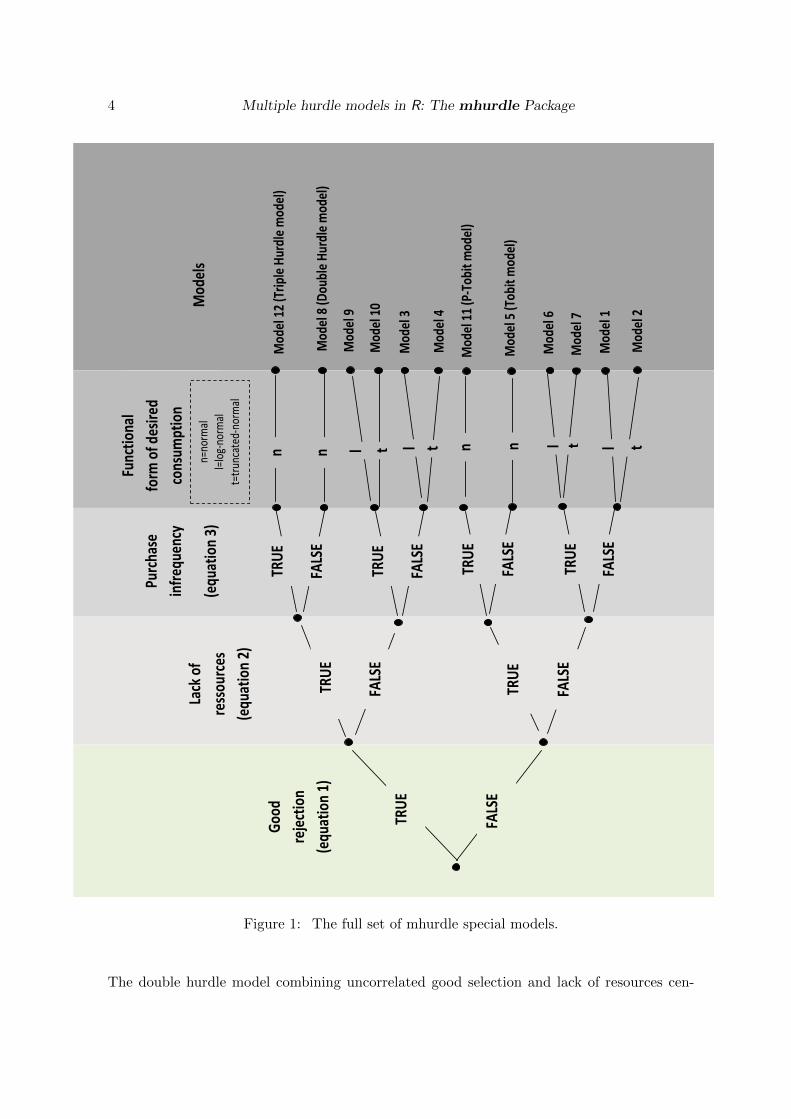
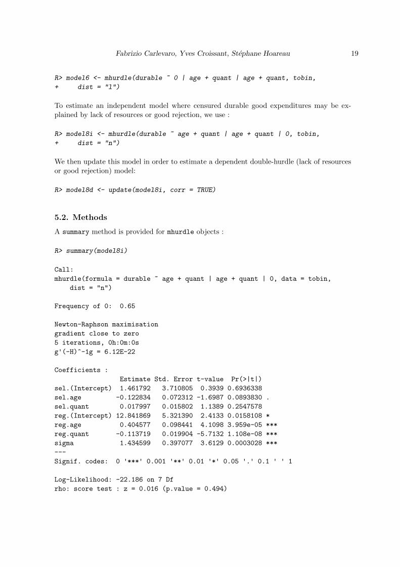