Embed Size (px)
Citation preview
Scientific Computing
M. Caliari
a.y. 2018/2019
Contents
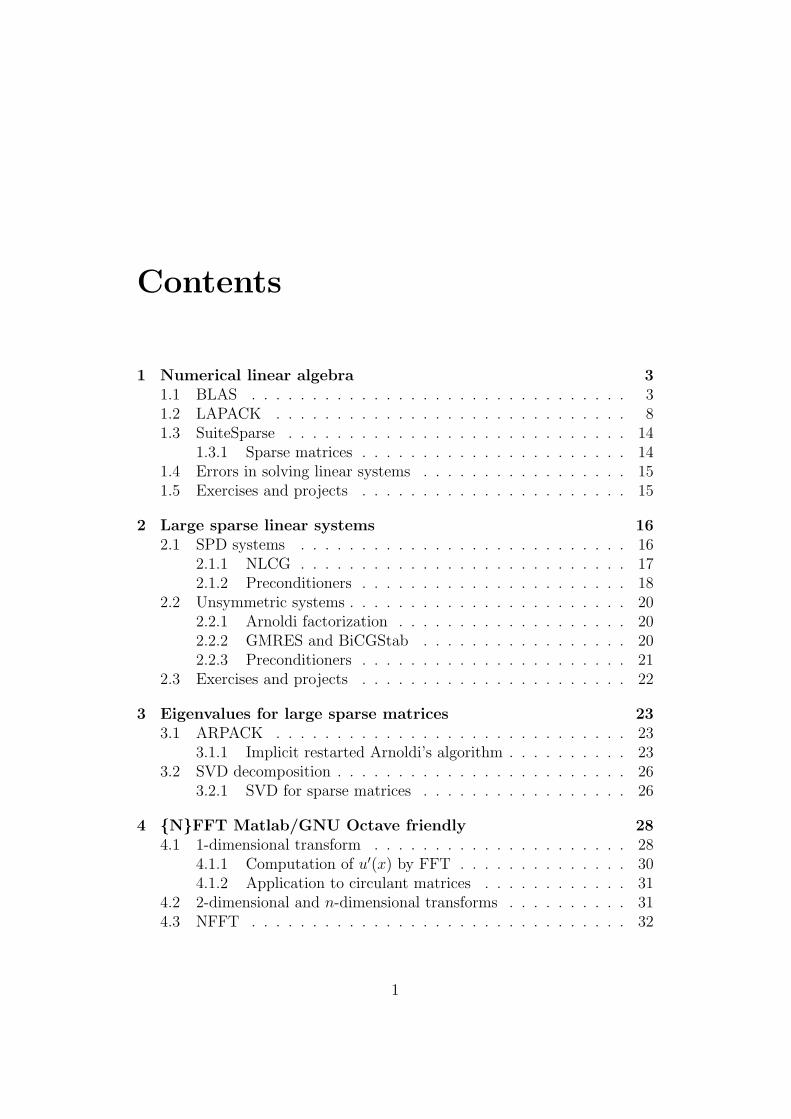
1 Numerical linear algebra 31.1 BLAS . . . . . . . . . . . . . . . . . . . . . . . . . . . . . . . 31.2 LAPACK . . . . . . . . . . . . . . . . . . . . . . . . . . . . . 81.3 SuiteSparse . . . . . . . . . . . . . . . . . . . . . . . . . . . . 14
1.3.1 Sparse matrices . . . . . . . . . . . . . . . . . . . . . . 141.4 Errors in solving linear systems . . . . . . . . . . . . . . . . . 151.5 Exercises and projects . . . . . . . . . . . . . . . . . . . . . . 15
2 Large sparse linear systems 162.1 SPD systems . . . . . . . . . . . . . . . . . . . . . . . . . . . 16
2.1.1 NLCG . . . . . . . . . . . . . . . . . . . . . . . . . . . 172.1.2 Preconditioners . . . . . . . . . . . . . . . . . . . . . . 18
2.2 Unsymmetric systems . . . . . . . . . . . . . . . . . . . . . . . 202.2.1 Arnoldi factorization . . . . . . . . . . . . . . . . . . . 202.2.2 GMRES and BiCGStab . . . . . . . . . . . . . . . . . 202.2.3 Preconditioners . . . . . . . . . . . . . . . . . . . . . . 21
2.3 Exercises and projects . . . . . . . . . . . . . . . . . . . . . . 22
3 Eigenvalues for large sparse matrices 233.1 ARPACK . . . . . . . . . . . . . . . . . . . . . . . . . . . . . 23
3.1.1 Implicit restarted Arnoldi’s algorithm . . . . . . . . . . 233.2 SVD decomposition . . . . . . . . . . . . . . . . . . . . . . . . 26
3.2.1 SVD for sparse matrices . . . . . . . . . . . . . . . . . 26
4 NFFT Matlab/GNU Octave friendly 284.1 1-dimensional transform . . . . . . . . . . . . . . . . . . . . . 28
4.1.1 Computation of u′(x) by FFT . . . . . . . . . . . . . . 304.1.2 Application to circulant matrices . . . . . . . . . . . . 31
4.2 2-dimensional and n-dimensional transforms . . . . . . . . . . 314.3 NFFT . . . . . . . . . . . . . . . . . . . . . . . . . . . . . . . 32
1
5 Finite Differences 335.1 1-dimensional . . . . . . . . . . . . . . . . . . . . . . . . . . . 33
5.1.1 Boundary conditions . . . . . . . . . . . . . . . . . . . 335.2 2-dimensional . . . . . . . . . . . . . . . . . . . . . . . . . . . 33
6 Finite Elements 356.1 Poisson problem . . . . . . . . . . . . . . . . . . . . . . . . . . 356.2 p-Laplace problem . . . . . . . . . . . . . . . . . . . . . . . . 36
6.2.1 Use of a preconditioner . . . . . . . . . . . . . . . . . . 376.3 Exercises and projects . . . . . . . . . . . . . . . . . . . . . . 38
7 Matrix functions 397.1 Matrix exponential . . . . . . . . . . . . . . . . . . . . . . . . 39
7.1.1 Taylor’s truncated series . . . . . . . . . . . . . . . . . 397.1.2 Eigenvalue decomposition . . . . . . . . . . . . . . . . 40
7.2 Matrix exponential-related functions . . . . . . . . . . . . . . 41
2
Chapter 1
Numerical linear algebra
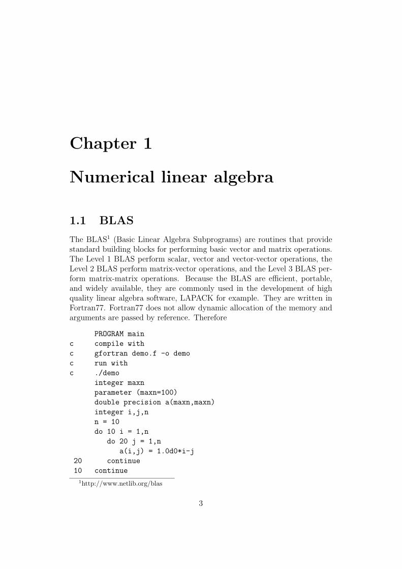
1.1 BLAS
The BLAS1 (Basic Linear Algebra Subprograms) are routines that providestandard building blocks for performing basic vector and matrix operations.The Level 1 BLAS perform scalar, vector and vector-vector operations, theLevel 2 BLAS perform matrix-vector operations, and the Level 3 BLAS per-form matrix-matrix operations. Because the BLAS are efficient, portable,and widely available, they are commonly used in the development of highquality linear algebra software, LAPACK for example. They are written inFortran77. Fortran77 does not allow dynamic allocation of the memory andarguments are passed by reference. Therefore
PROGRAM main
c compile with
c gfortran demo.f -o demo
c run with
c ./demo
integer maxn
parameter (maxn=100)
double precision a(maxn,maxn)
integer i,j,n
n = 10
do 10 i = 1,n
do 20 j = 1,n
a(i,j) = 1.0d0*i-j
20 continue
10 continue
1http://www.netlib.org/blas
3
call disp(a,maxn,n)
stop
end
SUBROUTINE disp(a,lda,n)
integer lda,n
double precision a(lda,n)
integer i,j
do 10 i = 1,n
write(6,’(10(1x,e8.2))’) (a(i,j),j=1,n)
10 continue
return
end
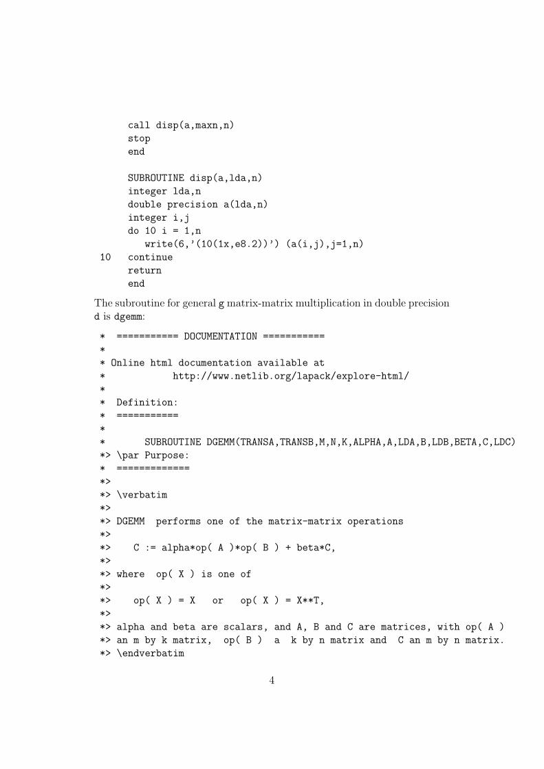
The subroutine for general gmatrix-matrix multiplication in double precisiond is dgemm:
* =========== DOCUMENTATION ===========
*
* Online html documentation available at
* http://www.netlib.org/lapack/explore-html/
*
* Definition:
* ===========
*
* SUBROUTINE DGEMM(TRANSA,TRANSB,M,N,K,ALPHA,A,LDA,B,LDB,BETA,C,LDC)
*> \par Purpose:
* =============
*>
*> \verbatim
*>
*> DGEMM performs one of the matrix-matrix operations
*>
*> C := alpha*op( A )*op( B ) + beta*C,
*>
*> where op( X ) is one of
*>
*> op( X ) = X or op( X ) = X**T,
*>
*> alpha and beta are scalars, and A, B and C are matrices, with op( A )
*> an m by k matrix, op( B ) a k by n matrix and C an m by n matrix.
*> \endverbatim
4
*
* Arguments:
* ==========
*
*> \param[in] TRANSA
*> \verbatim
*> TRANSA is CHARACTER*1
*> On entry, TRANSA specifies the form of op( A ) to be used in
*> the matrix multiplication as follows:
*>
*> TRANSA = ’N’ or ’n’, op( A ) = A.
*>
*> TRANSA = ’T’ or ’t’, op( A ) = A**T.
*>
*> TRANSA = ’C’ or ’c’, op( A ) = A**T.
*> \endverbatim
*>
*> \param[in] TRANSB
*> \verbatim
*> TRANSB is CHARACTER*1
*> On entry, TRANSB specifies the form of op( B ) to be used in
*> the matrix multiplication as follows:
*>
*> TRANSB = ’N’ or ’n’, op( B ) = B.
*>
*> TRANSB = ’T’ or ’t’, op( B ) = B**T.
*>
*> TRANSB = ’C’ or ’c’, op( B ) = B**T.
*> \endverbatim
*>
*> \param[in] M
*> \verbatim
*> M is INTEGER
*> On entry, M specifies the number of rows of the matrix
*> op( A ) and of the matrix C. M must be at least zero.
*> \endverbatim
*>
*> \param[in] N
*> \verbatim
*> N is INTEGER
*> On entry, N specifies the number of columns of the matrix
5
*> op( B ) and the number of columns of the matrix C. N must be
*> at least zero.
*> \endverbatim
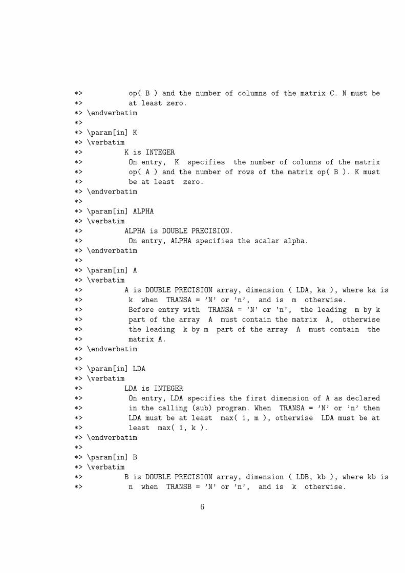
*>
*> \param[in] K
*> \verbatim
*> K is INTEGER
*> On entry, K specifies the number of columns of the matrix
*> op( A ) and the number of rows of the matrix op( B ). K must
*> be at least zero.
*> \endverbatim
*>
*> \param[in] ALPHA
*> \verbatim
*> ALPHA is DOUBLE PRECISION.
*> On entry, ALPHA specifies the scalar alpha.
*> \endverbatim
*>
*> \param[in] A
*> \verbatim
*> A is DOUBLE PRECISION array, dimension ( LDA, ka ), where ka is
*> k when TRANSA = ’N’ or ’n’, and is m otherwise.
*> Before entry with TRANSA = ’N’ or ’n’, the leading m by k
*> part of the array A must contain the matrix A, otherwise
*> the leading k by m part of the array A must contain the
*> matrix A.
*> \endverbatim
*>
*> \param[in] LDA
*> \verbatim
*> LDA is INTEGER
*> On entry, LDA specifies the first dimension of A as declared
*> in the calling (sub) program. When TRANSA = ’N’ or ’n’ then
*> LDA must be at least max( 1, m ), otherwise LDA must be at
*> least max( 1, k ).
*> \endverbatim
*>
*> \param[in] B
*> \verbatim
*> B is DOUBLE PRECISION array, dimension ( LDB, kb ), where kb is
*> n when TRANSB = ’N’ or ’n’, and is k otherwise.
6
*> Before entry with TRANSB = ’N’ or ’n’, the leading k by n
*> part of the array B must contain the matrix B, otherwise
*> the leading n by k part of the array B must contain the
*> matrix B.
*> \endverbatim
*>
*> \param[in] LDB
*> \verbatim
*> LDB is INTEGER
*> On entry, LDB specifies the first dimension of B as declared
*> in the calling (sub) program. When TRANSB = ’N’ or ’n’ then
*> LDB must be at least max( 1, k ), otherwise LDB must be at
*> least max( 1, n ).
*> \endverbatim
*>
*> \param[in] BETA
*> \verbatim
*> BETA is DOUBLE PRECISION.
*> On entry, BETA specifies the scalar beta. When BETA is
*> supplied as zero then C need not be set on input.
*> \endverbatim
*>
*> \param[in,out] C
*> \verbatim
*> C is DOUBLE PRECISION array, dimension ( LDC, N )
*> Before entry, the leading m by n part of the array C must
*> contain the matrix C, except when beta is zero, in which
*> case C need not be set on entry.
*> On exit, the array C is overwritten by the m by n matrix
*> ( alpha*op( A )*op( B ) + beta*C ).
*> \endverbatim
*>
*> \param[in] LDC
*> \verbatim
*> LDC is INTEGER
*> On entry, LDC specifies the first dimension of C as declared
*> in the calling (sub) program. LDC must be at least
*> max( 1, m ).
*> \endverbatim
*
* Authors:
7
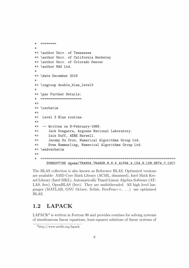
* ========
*
*> \author Univ. of Tennessee
*> \author Univ. of California Berkeley
*> \author Univ. of Colorado Denver
*> \author NAG Ltd.
*
*> \date December 2016
*
*> \ingroup double_blas_level3
*
*> \par Further Details:
* =====================
*>
*> \verbatim
*>
*> Level 3 Blas routine.
*>
*> -- Written on 8-February-1989.
*> Jack Dongarra, Argonne National Laboratory.
*> Iain Duff, AERE Harwell.
*> Jeremy Du Croz, Numerical Algorithms Group Ltd.
*> Sven Hammarling, Numerical Algorithms Group Ltd.
*> \endverbatim
*>
* =====================================================================
SUBROUTINE dgemm(TRANSA,TRANSB,M,N,K,ALPHA,A,LDA,B,LDB,BETA,C,LDC)
The BLAS collection is also known as Reference BLAS. Optimized versionsare available: AMD Core Math Library (ACML, dismissed), Intel Math Ker-nel Library (Intel MKL), Automatically Tuned Linear Algebra Software (AT-LAS, free), OpenBLAS (free). They are multithreaded. All high level lan-guages (MATLAB, GNU Octave, Scilab, FreeFem++, . . . ) use optimizedBLAS.
1.2 LAPACK
LAPACK2 is written in Fortran 90 and provides routines for solving systemsof simultaneous linear equations, least-squares solutions of linear systems of
2http://www.netlib.org/lapack
8
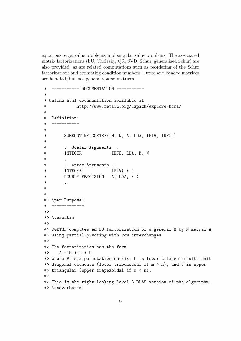
equations, eigenvalue problems, and singular value problems. The associatedmatrix factorizations (LU, Cholesky, QR, SVD, Schur, generalized Schur) arealso provided, as are related computations such as reordering of the Schurfactorizations and estimating condition numbers. Dense and banded matricesare handled, but not general sparse matrices.
* =========== DOCUMENTATION ===========
*
* Online html documentation available at
* http://www.netlib.org/lapack/explore-html/
*
* Definition:
* ===========
*
* SUBROUTINE DGETRF( M, N, A, LDA, IPIV, INFO )
*
* .. Scalar Arguments ..
* INTEGER INFO, LDA, M, N
* ..
* .. Array Arguments ..
* INTEGER IPIV( * )
* DOUBLE PRECISION A( LDA, * )
* ..
*
*
*> \par Purpose:
* =============
*>
*> \verbatim
*>
*> DGETRF computes an LU factorization of a general M-by-N matrix A
*> using partial pivoting with row interchanges.
*>
*> The factorization has the form
*> A = P * L * U
*> where P is a permutation matrix, L is lower triangular with unit
*> diagonal elements (lower trapezoidal if m > n), and U is upper
*> triangular (upper trapezoidal if m < n).
*>
*> This is the right-looking Level 3 BLAS version of the algorithm.
*> \endverbatim
9
*
* Arguments:
* ==========
*
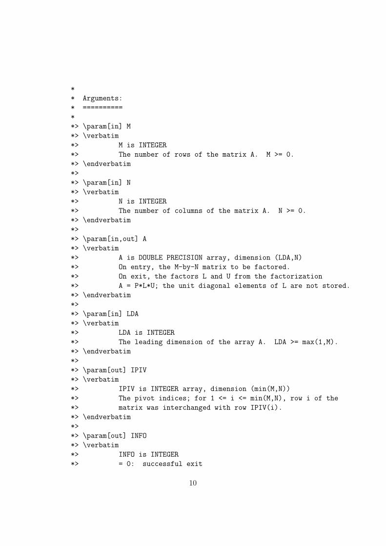
*> \param[in] M
*> \verbatim
*> M is INTEGER
*> The number of rows of the matrix A. M >= 0.
*> \endverbatim
*>
*> \param[in] N
*> \verbatim
*> N is INTEGER
*> The number of columns of the matrix A. N >= 0.
*> \endverbatim
*>
*> \param[in,out] A
*> \verbatim
*> A is DOUBLE PRECISION array, dimension (LDA,N)
*> On entry, the M-by-N matrix to be factored.
*> On exit, the factors L and U from the factorization
*> A = P*L*U; the unit diagonal elements of L are not stored.
*> \endverbatim
*>
*> \param[in] LDA
*> \verbatim
*> LDA is INTEGER
*> The leading dimension of the array A. LDA >= max(1,M).
*> \endverbatim
*>
*> \param[out] IPIV
*> \verbatim
*> IPIV is INTEGER array, dimension (min(M,N))
*> The pivot indices; for 1 <= i <= min(M,N), row i of the
*> matrix was interchanged with row IPIV(i).
*> \endverbatim
*>
*> \param[out] INFO
*> \verbatim
*> INFO is INTEGER
*> = 0: successful exit
10
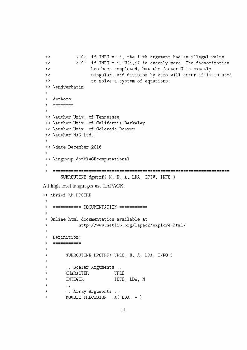
*> < 0: if INFO = -i, the i-th argument had an illegal value
*> > 0: if INFO = i, U(i,i) is exactly zero. The factorization
*> has been completed, but the factor U is exactly
*> singular, and division by zero will occur if it is used
*> to solve a system of equations.
*> \endverbatim
*
* Authors:
* ========
*
*> \author Univ. of Tennessee
*> \author Univ. of California Berkeley
*> \author Univ. of Colorado Denver
*> \author NAG Ltd.
*
*> \date December 2016
*
*> \ingroup doubleGEcomputational
*
* =====================================================================
SUBROUTINE dgetrf( M, N, A, LDA, IPIV, INFO )
All high level languages use LAPACK.
*> \brief \b DPOTRF
*
* =========== DOCUMENTATION ===========
*
* Online html documentation available at
* http://www.netlib.org/lapack/explore-html/
*
* Definition:
* ===========
*
* SUBROUTINE DPOTRF( UPLO, N, A, LDA, INFO )
*
* .. Scalar Arguments ..
* CHARACTER UPLO
* INTEGER INFO, LDA, N
* ..
* .. Array Arguments ..
* DOUBLE PRECISION A( LDA, * )
11
* ..
*
*
*> \par Purpose:
* =============
*>
*> \verbatim
*>
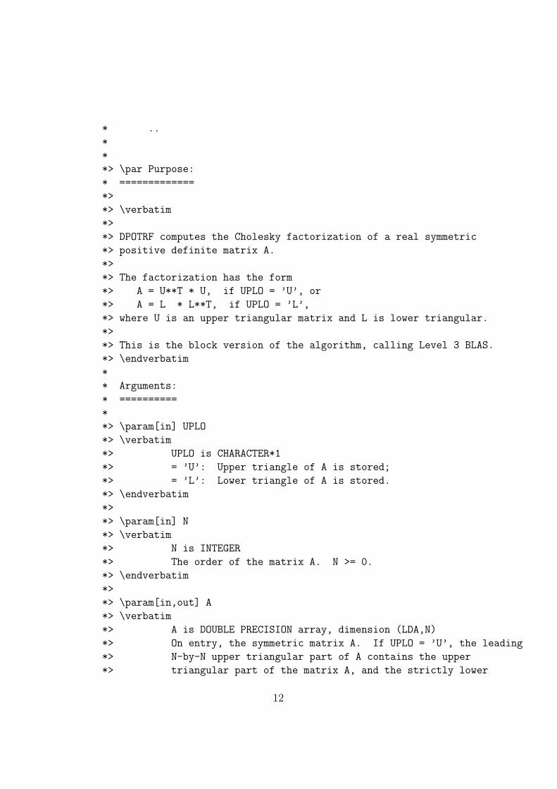
*> DPOTRF computes the Cholesky factorization of a real symmetric
*> positive definite matrix A.
*>
*> The factorization has the form
*> A = U**T * U, if UPLO = ’U’, or
*> A = L * L**T, if UPLO = ’L’,
*> where U is an upper triangular matrix and L is lower triangular.
*>
*> This is the block version of the algorithm, calling Level 3 BLAS.
*> \endverbatim
*
* Arguments:
* ==========
*
*> \param[in] UPLO
*> \verbatim
*> UPLO is CHARACTER*1
*> = ’U’: Upper triangle of A is stored;
*> = ’L’: Lower triangle of A is stored.
*> \endverbatim
*>
*> \param[in] N
*> \verbatim
*> N is INTEGER
*> The order of the matrix A. N >= 0.
*> \endverbatim
*>
*> \param[in,out] A
*> \verbatim
*> A is DOUBLE PRECISION array, dimension (LDA,N)
*> On entry, the symmetric matrix A. If UPLO = ’U’, the leading
*> N-by-N upper triangular part of A contains the upper
*> triangular part of the matrix A, and the strictly lower
12
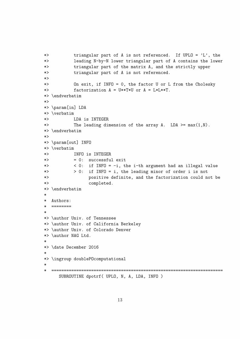
*> triangular part of A is not referenced. If UPLO = ’L’, the
*> leading N-by-N lower triangular part of A contains the lower
*> triangular part of the matrix A, and the strictly upper
*> triangular part of A is not referenced.
*>
*> On exit, if INFO = 0, the factor U or L from the Cholesky
*> factorization A = U**T*U or A = L*L**T.
*> \endverbatim
*>
*> \param[in] LDA
*> \verbatim
*> LDA is INTEGER
*> The leading dimension of the array A. LDA >= max(1,N).
*> \endverbatim
*>
*> \param[out] INFO
*> \verbatim
*> INFO is INTEGER
*> = 0: successful exit
*> < 0: if INFO = -i, the i-th argument had an illegal value
*> > 0: if INFO = i, the leading minor of order i is not
*> positive definite, and the factorization could not be
*> completed.
*> \endverbatim
*
* Authors:
* ========
*
*> \author Univ. of Tennessee
*> \author Univ. of California Berkeley
*> \author Univ. of Colorado Denver
*> \author NAG Ltd.
*
*> \date December 2016
*
*> \ingroup doublePOcomputational
*
* =====================================================================
SUBROUTINE dpotrf( UPLO, N, A, LDA, INFO )
13
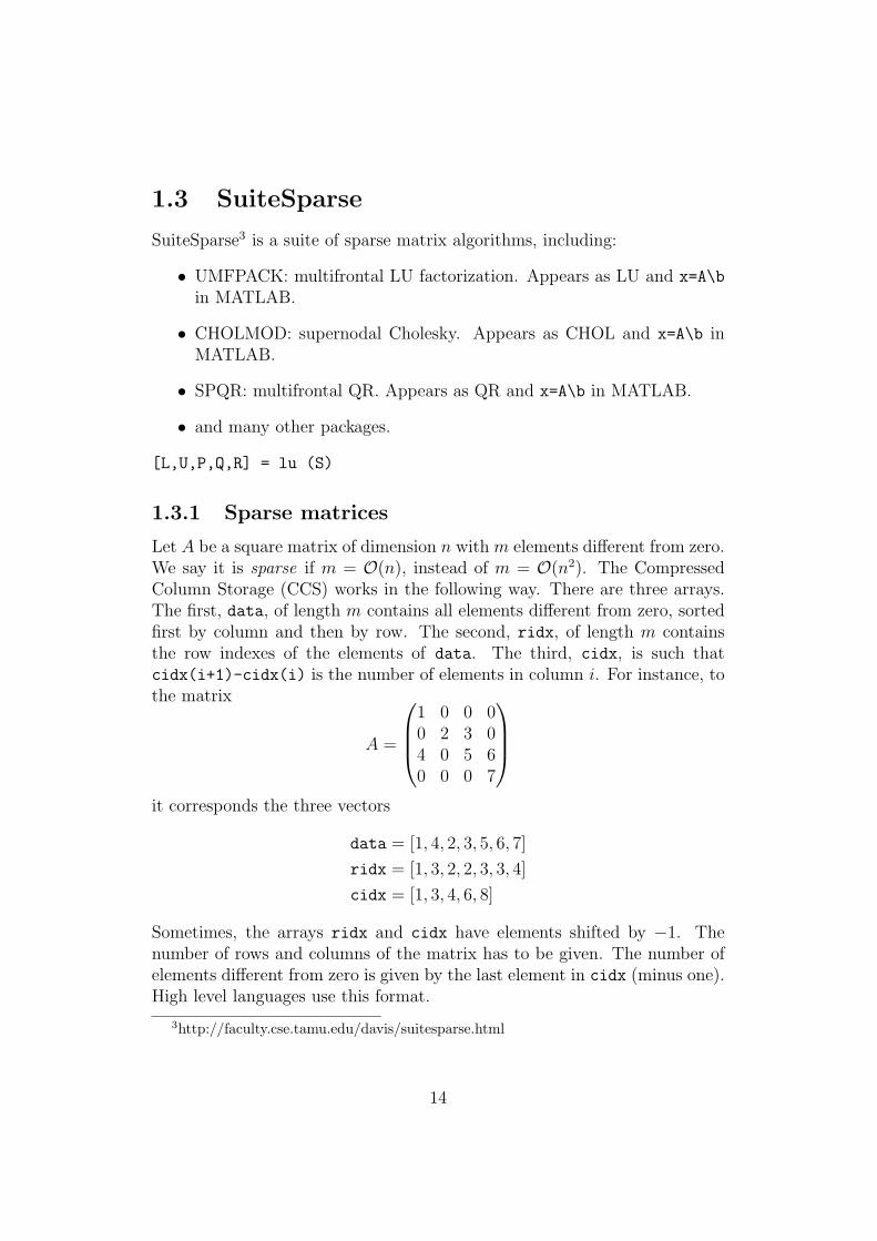
1.3 SuiteSparse
SuiteSparse3 is a suite of sparse matrix algorithms, including:
• UMFPACK: multifrontal LU factorization. Appears as LU and x=A\b
in MATLAB.
• CHOLMOD: supernodal Cholesky. Appears as CHOL and x=A\b inMATLAB.
• SPQR: multifrontal QR. Appears as QR and x=A\b in MATLAB.
• and many other packages.
[L,U,P,Q,R] = lu (S)
1.3.1 Sparse matrices
Let A be a square matrix of dimension n with m elements different from zero.We say it is sparse if m = O(n), instead of m = O(n2). The CompressedColumn Storage (CCS) works in the following way. There are three arrays.The first, data, of length m contains all elements different from zero, sortedfirst by column and then by row. The second, ridx, of length m containsthe row indexes of the elements of data. The third, cidx, is such thatcidx(i+1)-cidx(i) is the number of elements in column i. For instance, tothe matrix
A =
1 0 0 00 2 3 04 0 5 60 0 0 7
it corresponds the three vectors
data = [1, 4, 2, 3, 5, 6, 7]
ridx = [1, 3, 2, 2, 3, 3, 4]
cidx = [1, 3, 4, 6, 8]
Sometimes, the arrays ridx and cidx have elements shifted by −1. Thenumber of rows and columns of the matrix has to be given. The number ofelements different from zero is given by the last element in cidx (minus one).High level languages use this format.
3http://faculty.cse.tamu.edu/davis/suitesparse.html
14
1.4 Errors in solving linear systems
Suppose that a numerical method finds x such that r = b−Ax, the residual,is small. Then, we have
‖e‖‖x‖ =
‖x− x‖‖x‖ =
‖A−1((b− r)− b)‖‖x‖ =
‖A−1r‖‖x‖ ≤ ‖A−1‖‖r‖
‖x‖ ≤
≤ ‖A−1‖‖A‖‖r‖‖b‖ ≤ cond(A)
‖r‖‖b‖
1.5 Exercises and projects
1. Implement the function function w = matvec (data, ridx, cidx, v)
and w = matvect (data, ridx, cidx, v) which implement the sparse(transposed) matrix-vector products for square matrices.
2. Project: implement the function [L, U, P] = lu (data, ridx, cidx)
for LU factorization of a sparse matrix.
15
Chapter 2
Large sparse linear systems
Besides methods base on the SuiteSparse library (which are direct methods),it is possible to use iterative methods [7]. By iterative methods I mean Krylovmethods and not Jacobi, Gauss–Sidel, or SOR methods. It is difficult to saywhich class is better. The main advantage of iterative methods is that it ispossible to specify a tolerance for the error. Moreover, usually the entries ofthe matrix A are not required, but only the action of A (and possibly of AT )to a vector.
2.1 SPD systems
The most used method for symmetric (Hermitian) positive definite systemsis the Conjugate Gradient method. The idea is that, instead of solving thelinear system Ax = b, one tries to minimize the quadratic functional
J(x) =1
2xTAx− xT b
Starting from an initial guess x0, iterates are given by
xm = xm−1 + αm−1pm−1
where pm−1 is a “descent” direction. Given it, it is easy to determine αm−1:in fact
J(xm−1+αpm−1) =1
2xTm−1Axm−1−xTm−1b+α(p
Tm−1Axm−1−pTm−1b)+
1
2α2pTm−1Apm−1
and the minimum, in α, is taken by
αm−1 =pTm−1rm−1
pTm−1Apm−1
16
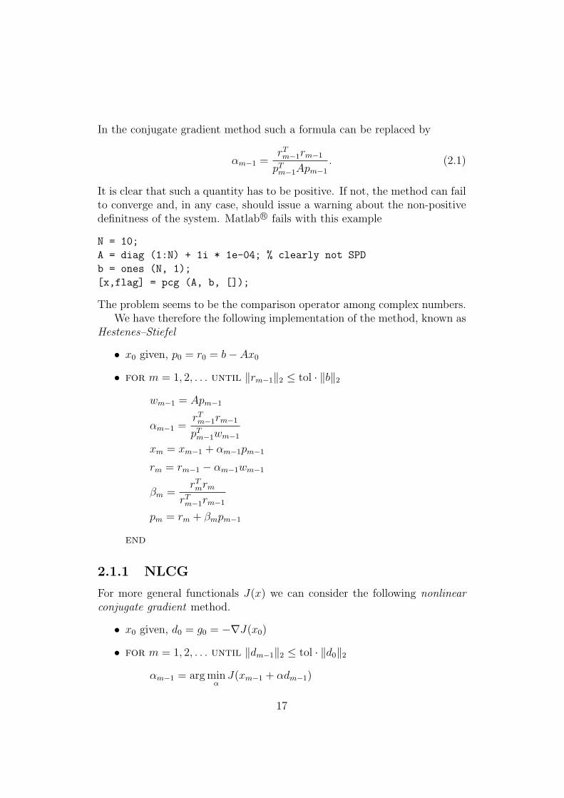
In the conjugate gradient method such a formula can be replaced by
αm−1 =rTm−1rm−1
pTm−1Apm−1
. (2.1)
It is clear that such a quantity has to be positive. If not, the method can failto converge and, in any case, should issue a warning about the non-positivedefinitness of the system. Matlab R© fails with this example
N = 10;
A = diag (1:N) + 1i * 1e-04; % clearly not SPD
b = ones (N, 1);
[x,flag] = pcg (A, b, []);
The problem seems to be the comparison operator among complex numbers.We have therefore the following implementation of the method, known as
Hestenes–Stiefel
• x0 given, p0 = r0 = b− Ax0
• for m = 1, 2, . . . until ‖rm−1‖2 ≤ tol · ‖b‖2wm−1 = Apm−1
αm−1 =rTm−1rm−1
pTm−1wm−1
xm = xm−1 + αm−1pm−1
rm = rm−1 − αm−1wm−1
βm =rTmrm
rTm−1rm−1
pm = rm + βmpm−1
end
2.1.1 NLCG
For more general functionals J(x) we can consider the following nonlinear
conjugate gradient method.
• x0 given, d0 = g0 = −∇J(x0)
• for m = 1, 2, . . . until ‖dm−1‖2 ≤ tol · ‖d0‖2αm−1 = argmin
αJ(xm−1 + αdm−1)
17
xm = xm−1 + αm−1dm−1
gm = −∇J(xm)
βm =gTm∇J(xm)
gTm−1∇J(xm−1)
dm = gm + βmdm−1
end
It is in general not necessary to compute exactly αm−1. In this case we speakabout inexact linesearch. It can be performed, for instance, by few steps ofgolden search of g(α) = J(xm−1 + αdm−1). Or it is possible to look for thezero of the univariate function dTm−1∇J(xm−1 + αdm−1). The choice of βmcorresponds to Fletcher–Reeves. NLCG is available in FreeFem++.
2.1.2 Preconditioners
The idea is to changeAx = b
intoP−1Ax = P−1b
in such a way that P−1A is better conditioned than A and the conjugategradient method faster (left preconditioning). The main problem for theCG algorithm is that even if P is SPD, P−1A is not SPD. We can thereforefactorize P into P = RTR and consider the linear system
P−1AR−1y = P−1b⇔ R−TAR−1y = R−T b, R−1y = x
Now, A = R−TAR−1 is SPD and we can solve the system Ay = b, b = R−T b,with the CG method. Setting xm = Rxm, we have rm = b− Axm = R−T b−R−TAxm = R−T rm. This is called split preconditioning. It is possible thento arrange the CG algorithm for A, x0 and b as
• x0 given, r0 = b− Ax0, Pz0 = r0, p0 = z0
• for m = 1, 2, . . . until ‖rm‖2 ≤ tol · ‖b‖2
wm−1 = Apm−1
αm−1 =zTm−1rm−1
pTm−1wm−1
xm = xm−1 + αm−1pm−1
18
rm = rm−1 − αm−1wm−1
Pzm = rm
βm =zTmrm
zTm−1rm−1
pm = zm + βmpm−1
end
The directions pm are still A conjugate directions (with Pp0 = r0). Thisalgorithm requires the solution of the linear system Pzm = rm at each itera-tion. From one side P should be as close as possibile to A, from the other itshould be easy to “invert”. The simplest choice is P = diag(A). It is calledJacobi preconditioner. This preconditioner is the default in FreeFem++. IfP is not diagonal, usually it is factorized once and for all into P = RTR, Rthe triangular Cholesky factor, in such a way that zm can be recovered bytwo simple triangular linear systems. A possibile choice is the incompleteCholesky factorization of A. That is, P = RT R ≈ A where
(A− RT R)ij = 0 if aij 6= 0
rij = 0 if aij = 0
The preconditioned Conjugate Gradient method does not explicitely requirethe entries of P , but only the action of P−1 (which can be R−1R−T ) toa vector zm (that is the solution of a linear system with matrix P ). Thedefinition of αm−1
αm−1 =rTm−1Prm−1
pTm−1Apm−1
(2.2)
now requires that both the numerator and the denomination be positive. Theusual way to call this method in matlab is
pcg (A, x, tol, maxit, M) % a preconditioner M easy to invert
pcg (A, x, tol, maxit, M1, M2) % a preconditioner M in the form M1 * M2
From Matlab R© documentation, it seems that a left preconditioner is used,but it is not true.
It is possible to apply a preconditioner to the nonlinear conjugate gradientmethod, too. In fact, suppose that −∇J(xm) is of type b− A(xm) for somefunction A : Rn → R
n. It is then possible to approximate A(x) with Amxand use the matrix Am (which is ∇(Amx)) as preconditioner and computegm as −A−1
m ∇J(xm). Instead of the matrix Am, in order to reduce the costof inverting it, can be replaced by Ap⌊m/p⌋, for p > 1 integer.
19
2.2 Unsymmetric systems
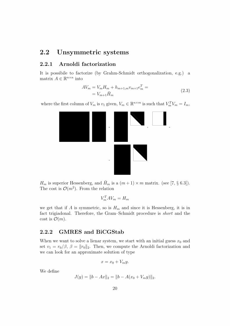
2.2.1 Arnoldi factorization
It is possibile to factorize (by Grahm-Schmidt orthogonalization, e.g.) amatrix A ∈ R
n×n into
AVm = VmHm + hm+1,mvm+1eTm =
= Vm+1Hm
(2.3)
where the first column of Vm is v1 given, Vm ∈ Rn×m is such that V T
mVm = Im,
+=
=
=
Hm is superior Hessenberg, and Hm is a (m+1)×m matrix. (see [7, § 6.3]).The cost is O(m2). From the relation
V TmAVm = Hm
we get that if A is symmetric, so is Hm and since it is Hessenberg, it is infact trigiadonal. Therefore, the Gram–Schmidt procedure is short and thecost is O(m).
2.2.2 GMRES and BiCGStab
When we want to solve a lienar system, we start with an initial guess x0 andset v1 = r0/β, β = ‖r0‖2. Then, we compute the Arnoldi factorization andwe can look for an approximate solution of type
x = x0 + Vmy.
We defineJ(y) = ‖b− Ax‖2 = ‖b− A(x0 + Vmy)‖2.
20
Moreover, we have
b− Ax = b− A(x0 + Vmy) =
= r0 − AVmy =
βv1 − Vm+1Hmy =
= Vm+1(βe1 − Hmy).
Therefore,J(y) = ‖βe1 − Hmy‖2
The GMRES methods attempts to minimize J and compute
ym = arg miny∈Rm
‖βe1 − Hmy‖2, xm = x0 + Vmym.
The linear system Hmy = βe1 is rectangular (over-determined) and it ispossible to find the least squares solution using the SVD decomposition.GMRES is available in FreeFem++.
Another popular method for general systems is BiCGStab. The maindifferences are:
• given the number of iterations m, the cost of GMRES is one matrix-vector product per iteration and m2 vector operations, while the cost ofBiCGStab is two matrix vector products per iteration (one with A andthe other with AT , even if AT is not required) and m vector operations
• GMRES uses a left preconditioner, while BiCGStab a right precondi-tioner (Ax = b ⇔ Ay = b, Px = y, Matlab documentation is con-fused).
2.2.3 Preconditioners
The basic code for the incomplete LU factorization is a very simple modifi-cation of the standard LU factorization.
n = length (A);
for k = 1:n - 1
for i = k + 1:n
if (A(i, k) ~= 0)
A(i, k) = A(i, k) / A(k, k);
for j = k + 1:n
if (A(i, j) ~= 0)
A(i, j) = A(i, j) - A(i, k) * A(k, j);
21
end
end
end
end
end
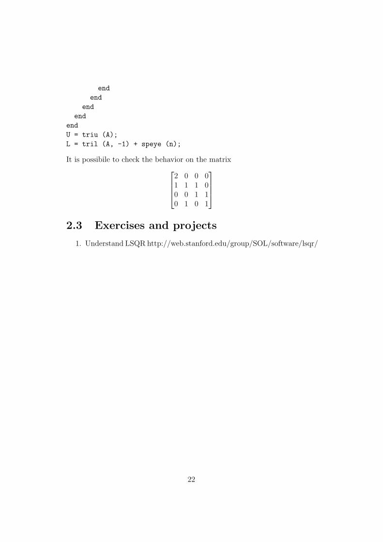
U = triu (A);
L = tril (A, -1) + speye (n);
It is possibile to check the behavior on the matrix
2 0 0 01 1 1 00 0 1 10 1 0 1
2.3 Exercises and projects
1. Understand LSQR http://web.stanford.edu/group/SOL/software/lsqr/
22
Chapter 3
Eigenvalues for large sparsematrices
The computation of eigenvalues and eigenvectors for “small” full matrices indone in LAPACK with optimized implmentations of the QR algorithm. TheQR algorithm is based on the QR factorization of a matrix. Any matrix canbe split according to
A = QR
withQ orthogonal and R upper triangular. The QR algorithm for eigenvaluesproduces a sequence
A0 = A = Q0R0, A1 = R0Q0 = Q1R1, A2 = R1Q1 = . . .
ClearlyAk+1 = RkQk = QT
kQkRkQk = QTkAkQk
and thus all the matrices in the sequence are similar and share the sameeigenvalues. Under some hypothesis, the limit of Ak for k → ∞ is an uppertriangular matrix whose eigenvalues are in the diagonal.
For large sparse matrices, several techniques are available.
3.1 ARPACK
3.1.1 Implicit restarted Arnoldi’s algorithm
Let us analyze the method under the popular ARPACK [6] package in For-tran77 for eigenvalue problems. It allows to compute “some” eigenvalues oflarge sparse matrices (such as the largest in magnitude, the smallest, . . . ).We start with an Arnoldi factorization (m≪ n)
V TmAVm = Hm
23
If (θ, s) is an eigenpair for Hm, that is Hms = θs, then
(v, Ax− θx) = 0, ∀v ∈ K
where x = Vms and K is the Krylov space spanned by the columns of Vm. Infact, v can be written as Vmy and therefore
(Vmy, Ax− θx) = yTV TmAVms− yTV T
mVmsθ = yT (Hms− θs) = 0
The couple (θ, x) is called Ritz pair and it is close to an eigenpair of A. Infact
‖Ax− θx‖2 = ‖(AVm − VmHm)s‖2 =∣
∣βmeTms∣
∣
where βm = ‖wm‖2. “In the Hermitian case, this estimate on the residualcan be turned into a precise statement about the accuracy of the Ritz valueθ as an approximation to the eigenvalue of A that is nearest to θ. However,an analogous statement in the non-Hermitian case is not possible withoutfurther information concerning nonnormality and defectiveness.” [6, p. 64].We can compute the eigenvalues of Hm, for instance by the QR method,and select an “unwanted” eigenvalue µm (which is an approximation of aneigenvalue µ of A). Then, we apply one iteration of shifted QR algorithm,that is
Hm − µmIm = Q1R1, H+m = R1Q1 + µmIm
Of course, Q1 is Hessenberg and Q1H+m = HmQ1. Now we right-multiply the
Arnoldi factorization, in order to get
AVmQ1 = VmHmQ1 + wmeTmQ1 (3.1)
With few manipulations
AVmQ1 = VmQ1H+m + wme
TmQ1
AVmQ1 = (VmQ1)(R1Q1 + µmIm) + wmeTmQ1
(A− µmIn)VmQ1 = (VmQ1)(R1Q1) + wmeTmQ1
(A− µmIn)Vm = VmQ1R1 + wmeTm
and by setting V +m = VmQ1, we have that the first column of the last expres-
sion is(A− µmIn)v1 = V +
mR1e1 = v+1 (eT1R1e1)
that is, the first column of V +m is a multiple of (A − µmIn)v1. If v1 was a
linear combination of the eigenvectors xj of A, then
v+1 ‖ (A− µmIn)v1 =∑
j
(αjλjxj − αjµmxj)
24
Since µm is close to a λj, v+1 lacks the component parallel to xj. Relation (3.1)
can be rewritten asAV +
m = V +mH
+m + wme
TmQ1
ans if we consider the first column, it is an Arnoldi factorization with a start-ing vector v+1 (which is of unitary norm) lacking the unwanted component.In practice, given the m eigenvalues of Hm, they are split into the k wantedand the p = m − k unwanted and p shifted QR decompositions (with eachof the unwanted eigenvalues) are performed. Then, the Arnoldi factorizationis right-multiplied by Q = Q1Q2 . . . Qp and the first k columns kept. Thisturns out to be an Arnoldi factorization. In fact
AV +m Im,k = AV +
k ,
where now V +m = VmQ, and
V +mH
+mIm,k = V +
k H+k + (V +
m ek+1hk+1,k)eTk
and, since the Qj are Hessenberg matrices, the last row of Q, that is eTmQ, hasthe first k−1 entries which are zero and then a value σ (and then somethingelse). Therefore
wmeTmQIm,k = wmσe
Tk
All together, the first k columns are
AV +k = V +
k H+k + w+
k eTk , w+
k = (V +m ek+1hk+1,k + wmσ)
that is an Arnoldi factorization applied to an initial vector lacking the un-wanted components. Then, the the factorization is continued up tom columns.
The easyest to compute eigenvalues with a Krylov methods are the largestin magnitute (as for the power method). Therefore, if some other eigevaluesare desired, it is necessary to apply proper transformations. Let us considerthe generalized problem
Ax = λMx
If we are interested into eigenvalues around σ, first we notice that
(A− σM)x = (λ− σ)Mx⇒ x = (λ− σ)(A− σM)−1Mx
from which
(A− σM)−1Mx = νx, ν =1
λ− σ
Therefore, if we apply the Krylov method (or the power method) to theoperator OP−1B = (A − σM)−1M we end up with the eigenvalues closer
25
to σ. In order to do that, we need to be able to solve linear systems with(A− σM) and multiply vectors with M .
High level languages use ARPACK, although Matlab moved to a Krylov–Schur method [8] inside its eigs function. Another possible method is de- show
Mat-labhelp
scribed here [2]. A gateway for the Jacobi–Davidson method is here1. Skew-symmetric matrices!
3.2 SVD decomposition
Let us start with the SVD decomposition. Given a matrix A ∈ Rm×n, it
is A = USV T , where U ∈ Rm×m and V ∈ R
n×n are orthogonal matricesand S ∈ R
m×n is “diagonal” with elements σi, i = 1, 2, . . . ,minm,n. Theelements σi satisfy σ1 ≥ σ2 ≥, . . . , σminm,n ≥ 0 and r among them arestrictly positive if r = rank(A). The values σi are called “singular values”of A and do coincide with the square roots of the eigenvalues of ATA. TheSVD decomposition in MATLAB is [U, S, V] = svd (A) and it is basedon LAPACK libraries.
3.2.1 SVD for sparse matrices
“Many problems in scientific computation require knowledge of a few of thelargest or smallest singular values of a matrix and associated left and rightsingular vectors. These problems include the approximation of a large matrixby a matrix of low rank, the computation of the null space of a matrix, totalleast-squares prolems, as well as tracking of signals” [3]. A simple approachis the following: it is possible to compute few eigenvalues of
Z =
[
0 AAT 0
]
In fact, from
Z
[
uv
]
= λ
[
uv
]
we getAv = λu, ATu = λv ⇒ ATAv = ATλu = λ2v.
Therefore, |λ| is a singular value of A. Notice that Z is a symmetric ma-trix (all eigenvalues are real) and if λ ∈ σ(Z), so is −λ (associated to the
1http://www.win.tue.nl/casa/research/scientificcomputing/topics/jd/
26

eigenvector [−u, v]T ). Therefore, we have
[
0 AAT 0
]
=
[
U −UV V
] [
S 00 −S
] [
UT V T
−UT V T
]
where if σ ∈ S, then σ ≥ 0, from which A = USV T . Since UUT + UUT = Iand V V T + V V T = I,
√2U and
√2V are orthogonal matrices.
27
Chapter 4
NFFT Matlab/GNU Octavefriendly
4.1 1-dimensional transform
We consider, for N even,
u(x) =
N/2−1∑
j=−N/2
uj+1+N/2eij2π(x−a)/(b−a)
√b− a
=
=N∑
j=1
ujei(j−1−N/2)2π(x−a)/(b−a)
√b− a
=N∑
j=1
ujφj(x)
(4.1)
where uj is the approximation by trapezoidal quadrature rule of
∫ b
a
u(x)φj(x)dx
(we assume u(x) periodic in [a, b]) that is
uj =
∫ b
a
u(x)φj(x)dx =√b− a
∫ 1
0
u(a+ y(b− a))e−i(j−1)2πyeiNπydy ≈
≈√b− a
N
N∑
n=1
(
u(xn)eiNπyn
)
e−i(j−1)2πyn = uj
where yn = (n− 1)/N and xn = a+ (b− a)yn. We say that the 0 frequencyis in the center of spectrum. What is written in the box is the result of fft
28
([u(x1)eiNπy1 , . . . , u(xN )e
iNπyN ] ). We consider now, for 1 ≤ j ≤ N/2,
fft ([u(x1), . . . , u(xN )])j =N∑
n=1
u(xn)e−i(j−1)2πyn =
=N∑
n=1
(
u(xn)eiNπyn
)
e−i(N/2+j−1)2πyn =N√b− a
uN/2+j
and, for N/2 < j ≤ N ,
fft ([u(x1), . . . , u(xN )])j =N∑
n=1
u(xn)e−i(j−1)2πyn =
=N∑
n=1
(
u(xn)eiNπyn
)
e−i(j−N/2−1)2πyn =N√b− a
uj−N/2
taking into account that eiN2πyn = 1. Therefore uhat = fftshift (fft
(u)) * sqrt (b - a) / N. Then we have
ˆvn =N∑
k=1
vkφk(xn) =N∑
k=1
vkei(k−1−N/2)2π(xn−a)/(b−a)
√b− a
=
=N√b− a
1
N
(
N∑
k=1
vkei(k−1)2πyn
)
e−iNπyn
What written in the box is the result of ifft (vhat). We observe thate−iNπyn = (−1)n+1. We consider now
N∑
k=1
ifftshift ([v1, . . . , vN ])kei(k−1)2πyn =
N/2∑
k=1
vN/2+kei(k−1)2πyn +
N∑
k=N/2+1
vk−N/2ei(k−1)2πyn =
=N∑
k=N/2+1
vkei(k−N/2−1)2πyn +
N/2∑
k=1
vkei(N/2+k−1)2πyn =
= (−1)n+1
N/2∑
k=1
vkei(k−1)2πyn + (−1)n+1
N∑
k=N/2+1
vkei(k−1)2πyn =
=
(
N∑
k=1
vkei(k−1)2πyn
)
e−iNπyn
29
Therefore, vhathat=ifft (ifftshift (vhat)) * N / sqrt (b - a). Itis not difficult to prove that
u(xn) = u(xn)
that is, u(x) is an approximation of u(x) which interpolates u(x) at xn,n = 1, 2, . . . , N . The advantage of using the FFT algorithm (over a standardmatrix-vector product) is that its cost is O(N logN) instead of O(N2). Theuse of the scaling factor sqrt (b - a) / N has the following purpose. Withthe definition (4.1), we have
∫ b
a
|u(x)|2 dx =∞∑
j=−∞
|uj|2
(Parseval’s identity), withouth any scaling factor. When we replace the seriesby a sum, what happens in practice is
∫ b
a
|u(x)|2 dx ≈ b− a
N
N∑
n=1
|u(xn)|2 =N∑
j=1
|uj|2 .
The three main common mistakes when using FFT in Matlab are
• to forget to remove the last point from x = linspace (a, b, N + 1)
• to use the transpose conjugate operator ’ (single quote) to simply trans-pose a vector, while the operator .’ was probably what needed.
• to use i for the imaginary unit and then to overwrite it. Use 1i instead.
4.1.1 Computation of u′(x) by FFT
We have
u′(x) ≈(
N∑
j=1
ujφj(x)
)′
=N∑
j=1
ujφ′j(x) =
N∑
j=1
ujλjφj(x)
where λj = i(j− 1−N/2)2π/(b− a). You can try the following Matlab code
a = -2;
b = 2;
N = 32;
x = linspace(a,b,N+1)’;
x = x(1:N);
30
u = 1./(sin(2*pi*(x-a)/(b-a))+2);
u1 = -cos(2*pi*(x-a)/(b-a))*2*pi/(b-a)./(sin(2*pi*(x-a)/(b-a))+2).^2;
uhat = fftshift(fft(u))*sqrt(b-a)/N;
lambda = 1i*(-N/2:N/2-1)’*2*pi/(b-a);
vhat = uhat.*lambda;
vhathat = ifft(ifftshift(vhat))*N/sqrt(b-a);
norm(vhathat-u1,inf)
4.1.2 Application to circulant matrices
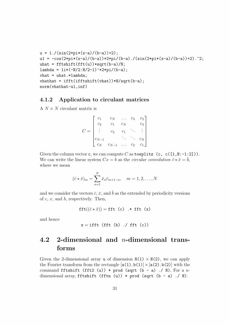
A N ×N circulant matrix is
C =
c1 cN . . . c3 c2c2 c1 cN c3... c2 c1
. . ....
cN−1. . . . . . cN
cN cN−1 . . . c2 c1
Given the column vector c, we can compute C as toeplitz (c, c([1,N:-1:2])).We can write the linear system Cx = b as the circular convolution c ⋆ x = b,where we mean
(c ⋆ x)m =N∑
n=1
xncm+1−n, m = 1, 2, . . . , N
and we consider the vectors c, x, and b as the extended by periodicity versionsof c, x, and b, respectively. Then,
fft((c ⋆ x)) = fft (c) .* fft (x)
and hencex = ifft (fft (b) ./ fft (c))
4.2 2-dimensional and n-dimensional trans-
forms
Given the 2-dimensional array u of dimension N(1) × N(2), we can applythe Fourier transform from the rectangle [a(1), b(1)]× [a(2), b(2)] with thecommand fftshift (fft2 (u)) * prod (sqrt (b - a) ./ N). For a n-dimensional array, fftshift (fftn (u)) * prod (sqrt (b - a) ./ N).
31
4.3 NFFT
The Nonuniform Fast Fourier Transform aims at being fast (O(N logN)) inevaluating a truncated Fourier series at a set of N general points. In fact,given the set of points xnNn=1, one could compute the matrix
Φ = (φj(xk))
and evaluate
u(x1)u(x2)...
u(xN)
= Φ
u1u2...uN
.
This would cost O(N2). The NFFT algorithm developed in [5] works in thefollowing way. It evaluates in a fast (and approximate) way a sum of type
N/2−1∑
j=−N/2
ψje−2πijξn , ξn ∈
[
−1
2,1
2
)
.
It is clear that we have to manipulate it in order to evaluate a sum oftype (4.1), with xn ∈ [a, b). In fact, the NFFT algorithm has to be fedwith
ξn = mod
(
xn − a
b− a, 1
)
− 1
2
ψj = ujeπi(j−1−N/2)
√b− a
= uj(−1)j−1−N/2
√b− a
Paper [4] contains a library for an easy integration and usage of NFFT (upto dimension 3) in Matlab/GNU Octave.
32
Chapter 5
Finite Differences
5.1 1-dimensional
On x = linspace (a, b, n)’, with h = (b - a) / (n - 1) we can con-struct the discretization matrices of first derivative and second derivative
Dx = toeplitz (sparse (1, 2, -1 / (2 * h), 1, n), ...
sparse (1, 2, 1 / (2 * h), 1, n));
Dxx = toeplitz (sparse ([1, 1], [1, 2], [-2, 1] / h ^ 2, 1, n));
5.1.1 Boundary conditions
Dirichlet b.c.
Periodic b.c.
Neumann b.c.
5.2 2-dimensional
Let’s check how to construct a grid in Matlab/GNU Octave.
x = linspace (a, b, n)’;
hx = (b - a) / (n - 1);
Dx = toeplitz (sparse (1, 2, -1 / (2 * hx), 1, n), ...
sparse (1, 2, 1 / (2 * hx), 1, n));
Dxx = toeplitz (sparse ([1, 1], [1, 2], [-2, 1] / hx ^ 2, 1, n));
y = linspace (c, d, m)’;
hy = (d - c) / (m - 1);
Dy = toeplitz (sparse (1, 2, -1 / (2 * hy), 1, m), ...
33
sparse (1, 2, 1 / (2 * hy), 1, m));
Dyy = toeplitz (sparse ([1, 1], [1, 2], [-2, 1] / hy ^ 2, 1, m));
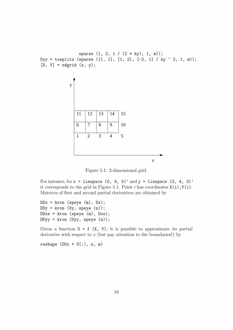
[X, Y] = ndgrid (x, y);
1 2 3 4 5
6 7 8 9 10
11 12 13 14 15
y
x
Figure 5.1: 2-dimensional grid.
For instance, for x = linspace (0, 4, 5)’ and y = linspace (2, 4, 3)’
it corresponds to the grid in Figure 5.1. Point i has coordinates X(i),Y(i).Matrices of first and second partial derivatives are obtained by
DDx = kron (speye (m), Dx);
DDy = kron (Dy, speye (n));
DDxx = kron (speye (m), Dxx);
DDyy = kron (Dyy, speye (n));
Given a function U = f (X, Y), it is possible to approximate its partialderivative with respect to x (but pay attention to the boundaries!) by
reshape (DDx * U(:), n, m)
34
Chapter 6
Finite Elements
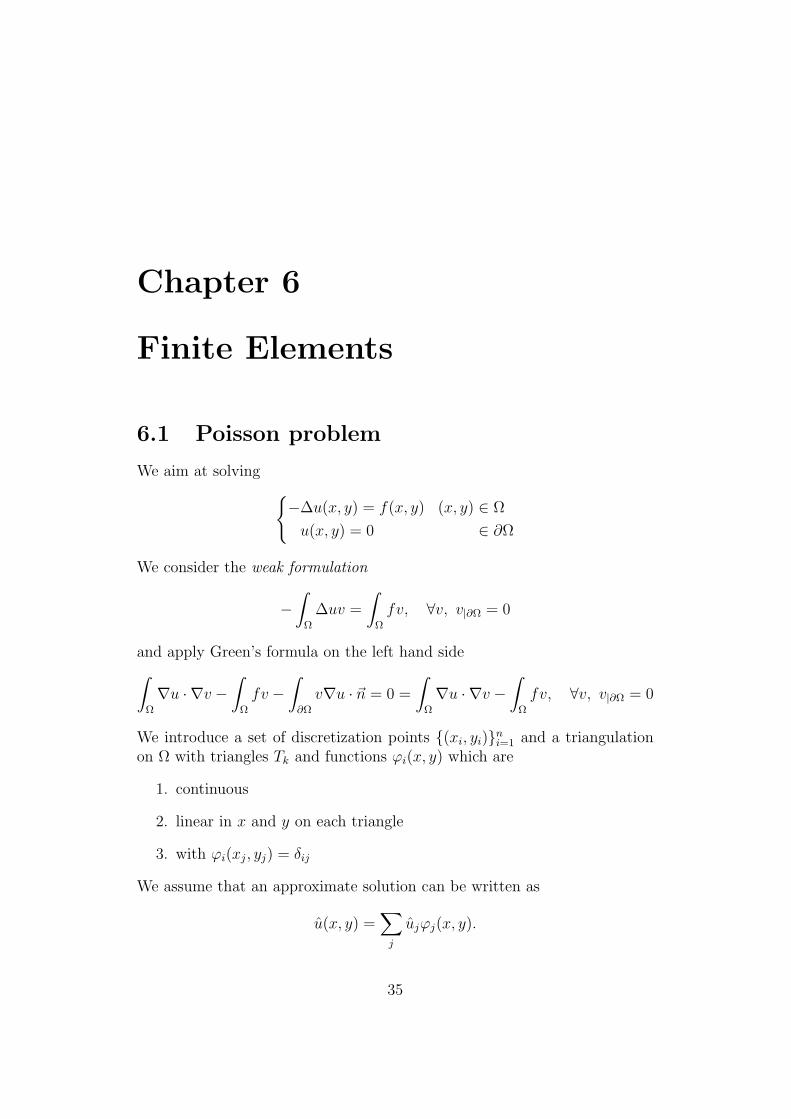
6.1 Poisson problem
We aim at solving
−∆u(x, y) = f(x, y) (x, y) ∈ Ω
u(x, y) = 0 ∈ ∂Ω
We consider the weak formulation
−∫
Ω
∆uv =
∫
Ω
fv, ∀v, v|∂Ω = 0
and apply Green’s formula on the left hand side
∫
Ω
∇u · ∇v −∫
Ω
fv −∫
∂Ω
v∇u · ~n = 0 =
∫
Ω
∇u · ∇v −∫
Ω
fv, ∀v, v|∂Ω = 0
We introduce a set of discretization points (xi, yi)ni=1 and a triangulationon Ω with triangles Tk and functions ϕi(x, y) which are
1. continuous
2. linear in x and y on each triangle
3. with ϕi(xj, yj) = δij
We assume that an approximate solution can be written as
u(x, y) =∑
j
ujϕj(x, y).
35
We insert such an approximation into the equation and get∫
Ω
∇u · ∇v −∫
Ω
fv = 0, ∀v, v|∂Ω = 0 (6.1)
where by ∇u we mean the piecewise gradient of u. The first term is a bilinearform on u and v and the second a linear form on v (that is a trivial bilinearform on nothing and v). If we insert the definitions of u and consider all theϕi instead of all the v, we get
∑
j
uj
(
∑
k
∫
Tk
∇ϕj · ∇ϕi
)
−(
∑
k
∫
Tk
fϕi
)
, ∀ϕi.
This is a linear system in the unknowns uj. Formulation (6.1) can be solvedby FreeFem++.
Another possibility it to look for the minimum of the functional
J(u) =1
2
∫
Ω
|∇u|2 −∫
Ω
fu.
In fact, a critical point for J is
δJ(u)v =
∫
Ω
∇u · ∇v −∫
Ω
fv = 0, ∀v, v|∂Ω = 0
Of course, we have to restrict the search in the finite dimensional space andlook for
u = arg minv, v|∂Ω=0
J(v)
6.2 p-Laplace problem
Now we consider the solution of
−div(|∇u|p−2 ∇u) = f Ω
u = 0 ∂Ω
for p ≥ 2. This problem is the Poisson problem for p = 2. The correspondingJ functional is
J(u) =1
p
∫
Ω
|∇u|p −∫
Ω
fu.
In FreeFem++ it possible to use the nonlinear conjugate gradient method tofind
u = arg minv, v|∂Ω=0
J(v).
36
It is necessary to compute
δJ(u)v =
∫
Ω
|∇u|p−2 ∇u · ∇v −∫
Ω
fv =
∫
Ω
(∇u · ∇u) p−2
2 ∇u · ∇v −∫
Ω
fv.
Since u =∑
j ujϕj and v =∑
i viϕi, it is possible to introduce the functionalδJR(u) : R
n → R defined by
δJR(u)v =
∫
Ω
∣
∣
∣
∣
∣
∑
j
uj∇ϕj
∣
∣
∣
∣
∣
p−2∑
j
uj∇ϕj ·∑
i
vi∇ϕi −∫
Ω
f∑
i
viϕi =
=∑
i
vi
∫
Ω
∣
∣
∣
∣
∣
∑
j
uj∇ϕj
∣
∣
∣
∣
∣
p−2∑
j
uj∇ϕj · ∇ϕi −∫
Ω
fϕi
.
Another way to write it is vT δJR(u). By the nonlinear conjugate gradient
method (NLCG in FreeFem++) it is possible to solve
u = argminv
JR(v).
Only the action of δJR(u) is required.
6.2.1 Use of a preconditioner
In a minimization method, a sequence umm is produced which tries tominimize JR defined by
JR(u) =1
p
∫
Ω
∣
∣
∣
∣
∣
∑
j
uj∇ϕj
∣
∣
∣
∣
∣
p
−∫
Ω
f∑
j
ujϕj
From the definition of δJR(u), we see that it is of type A(u) − b ∈ Rn. At
iteration m, its i-th component can be approximated by
∫
Ω
∣
∣
∣
∣
∣
∑
j
umj ∇ϕj
∣
∣
∣
∣
∣
p−2∑
j
uj∇ϕj · ∇ϕi −∫
Ω
fϕi =
=∑
j
uj
∫
Ω
∣
∣
∣
∣
∣
∑
j
umj ∇ϕj
∣
∣
∣
∣
∣
p−2
∇ϕj · ∇ϕi
−∫
Ω
fϕi
in such a way that the approximate differential can be casted as
Amu− b,
with Am a symmetric matrix. Well, Am, which is δ(Amu) (which is an
approximation of δ(A(u)− b)) is a preconditioner.
37

6.3 Exercises and projects
1. Write a FreeFem++ code which solve the p-Laplace problem for p upto 1000.
38
Chapter 7
Matrix functions
7.1 Matrix exponential
The matrix exponential for A ∈ Cn×n is defined as
exp(A) =∞∑
k=0
Ak
k!
In order to numerically evaluate it, we may think to two simple strategies:Taylor’s truncated series and eigenvalue decomposition.
7.1.1 Taylor’s truncated series
It is a strong temptation to approximate
exp(A) ≈m∑
k=0
Ak
k!= Tm(A)
Unfortunately, it does not work, even in simple scalar cases (try to com-pute the relative error e100(e−100 − Tm(−100)) for increasing values of m).The problem is that Taylor’s series, although everywhere convergent, is fastenough (that is it converges to machine precision before truncation errorsshow up) only in a neighborhood of 0. To this aim, the scaling and squaring
technique may help. That is, taken s = 2j such that ‖A‖ < 1, E = exp(A/s)is approximated by Tm(A/s) and later exp(A) is recovered by
E = E2 j times
39
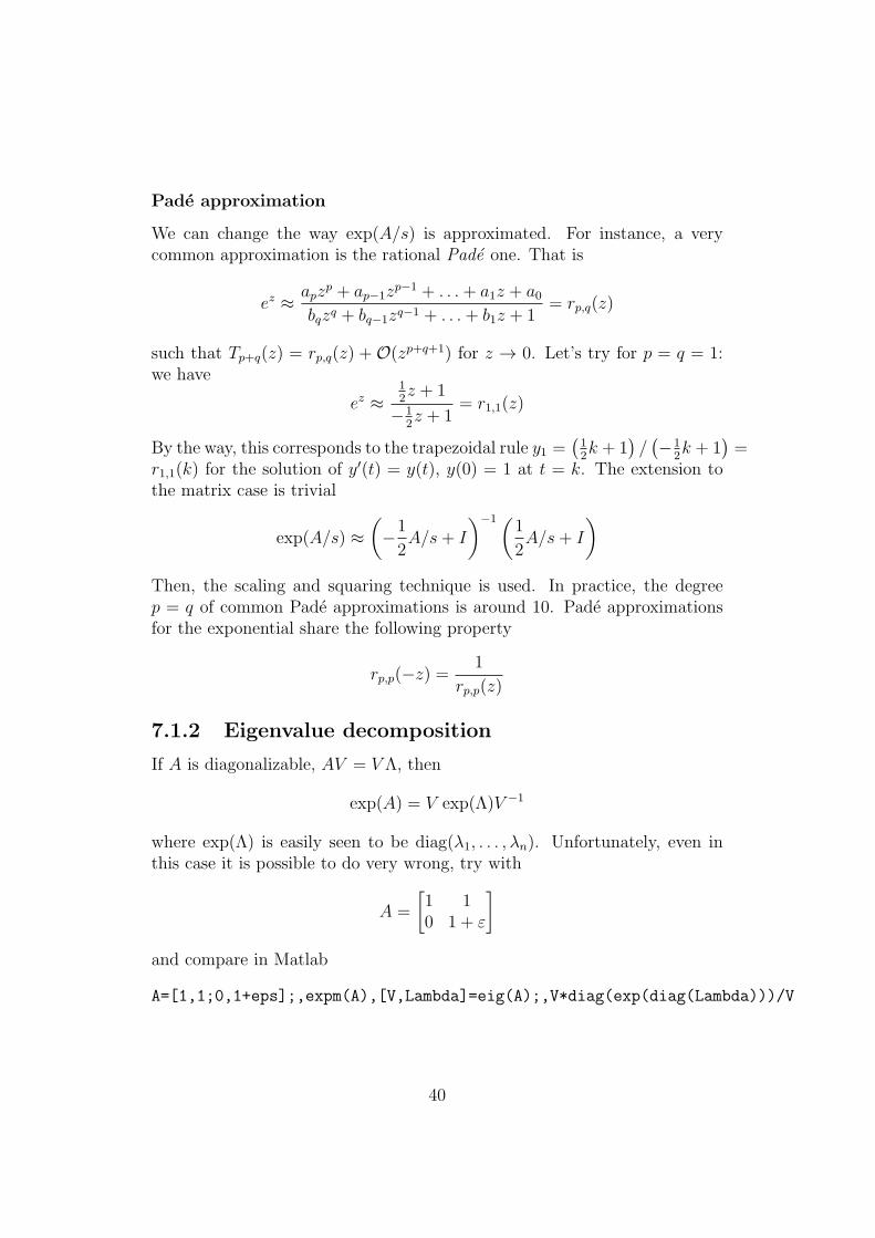
Pade approximation
We can change the way exp(A/s) is approximated. For instance, a verycommon approximation is the rational Pade one. That is
ez ≈ apzp + ap−1z
p−1 + . . .+ a1z + a0bqzq + bq−1zq−1 + . . .+ b1z + 1
= rp,q(z)
such that Tp+q(z) = rp,q(z) + O(zp+q+1) for z → 0. Let’s try for p = q = 1:we have
ez ≈12z + 1
−12z + 1
= r1,1(z)
By the way, this corresponds to the trapezoidal rule y1 =(
12k + 1
)
/(
−12k + 1
)
=r1,1(k) for the solution of y′(t) = y(t), y(0) = 1 at t = k. The extension tothe matrix case is trivial
exp(A/s) ≈(
−1
2A/s+ I
)−1(1
2A/s+ I
)
Then, the scaling and squaring technique is used. In practice, the degreep = q of common Pade approximations is around 10. Pade approximationsfor the exponential share the following property
rp,p(−z) =1
rp,p(z)
7.1.2 Eigenvalue decomposition
If A is diagonalizable, AV = V Λ, then
exp(A) = V exp(Λ)V −1
where exp(Λ) is easily seen to be diag(λ1, . . . , λn). Unfortunately, even inthis case it is possible to do very wrong, try with
A =
[
1 10 1 + ε
]
and compare in Matlab
A=[1,1;0,1+eps];,expm(A),[V,Lambda]=eig(A);,V*diag(exp(diag(Lambda)))/V
40
7.2 Matrix exponential-related functions
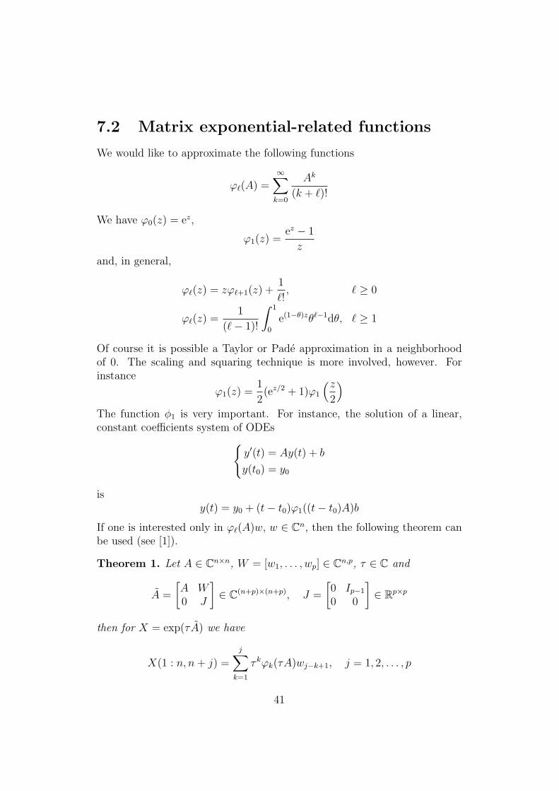
We would like to approximate the following functions
ϕℓ(A) =∞∑
k=0
Ak
(k + ℓ)!
We have ϕ0(z) = ez,
ϕ1(z) =ez − 1
z
and, in general,
ϕℓ(z) = zϕℓ+1(z) +1
ℓ!, ℓ ≥ 0
ϕℓ(z) =1
(ℓ− 1)!
∫ 1
0
e(1−θ)zθℓ−1dθ, ℓ ≥ 1
Of course it is possible a Taylor or Pade approximation in a neighborhoodof 0. The scaling and squaring technique is more involved, however. Forinstance
ϕ1(z) =1
2(ez/2 + 1)ϕ1
(z
2
)
The function φ1 is very important. For instance, the solution of a linear,constant coefficients system of ODEs
y′(t) = Ay(t) + b
y(t0) = y0
isy(t) = y0 + (t− t0)ϕ1((t− t0)A)b
If one is interested only in ϕℓ(A)w, w ∈ Cn, then the following theorem can
be used (see [1]).
Theorem 1. Let A ∈ Cn×n, W = [w1, . . . , wp] ∈ C
n,p, τ ∈ C and
A =
[
A W0 J
]
∈ C(n+p)×(n+p), J =
[
0 Ip−1
0 0
]
∈ Rp×p
then for X = exp(τA) we have
X(1 : n, n+ j) =
j∑
k=1
τ kϕk(τA)wj−k+1, j = 1, 2, . . . , p
41
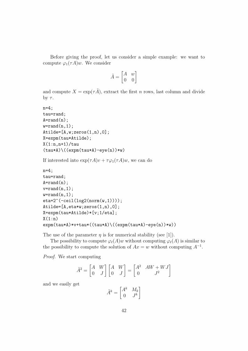
Before giving the proof, let us consider a simple example: we want tocompute ϕ1(τA)w. We consider
A =
[
A w0 0
]
and compute X = exp(τA), extract the first n rows, last column and divideby τ .
n=4;
tau=rand;
A=rand(n);
w=rand(n,1);
Atilde=[A,w;zeros(1,n),0];
X=expm(tau*Atilde);
X(1:n,n+1)/tau
(tau*A)\((expm(tau*A)-eye(n))*w)
If interested into exp(τA)v + τϕ1(τA)w, we can do
n=4;
tau=rand;
A=rand(n);
v=rand(n,1);
w=rand(n,1);
eta=2^(-ceil(log2(norm(w,1))));
Atilde=[A,eta*w;zeros(1,n),0];
X=expm(tau*Atilde)*[v;1/eta];
X(1:n)
expm(tau*A)*v+tau*((tau*A)\((expm(tau*A)-eye(n))*w))
The use of the parameter η is for numerical stability (see [1]).The possibility to compute ϕℓ(A)w without computing ϕℓ(A) is similar to
the possibility to compute the solution of Ax = w without computing A−1.
Proof. We start computing
A2 =
[
A W0 J
] [
A W0 J
]
=
[
A2 AW +WJ0 J2
]
and we easily get
Ak =
[
Ak Mk
0 Jk
]
42
with M0 = 0, M1 = W , Mk = Ak−1W +Mk−1J . Then WJ(:, j) = wj−1 andJJ(:, j) = J(:, j − 1) for 1 ≤ j ≤ p where we define w0 = J(:, 0) = 0. Thus
Mk(:, j) = Ak−1wj + (Ak−2W +Mk−2J)J(:, j) =
= Ak−1wj + Ak−2wj−1 +Mk−2J(:, j − 1) =
=
mink,j∑
i=1
Ak−iwj−i+1
Moreover
X(1 : n, n+ 1 : n+ p) =∞∑
k=0
τ kMk
k!=
∞∑
k=1
τ kMk
k!
and now we can compute
X(1 : n, n+ j) =∞∑
k=1
τ kMk(:, j)
k!=
∞∑
k=1
1
k!
minj,k∑
i=1
τ i(τA)k−iwj−i+1
=
=
j∑
i=1
τ i
(
∞∑
k=i
(τA)k−i
k!
)
wj−i+1 =
=
j∑
i=1
τ i
(
∞∑
k=0
(τA)k
(k + i)!
)
wj−i+1 =
j∑
i=1
τ iϕi(τA)wj−i+1
43
Bibliography
[1] A. H. Al-Mohy and N. J. Higham. Computing the action of the matrixexponential with an application to exponential integrators. SIAM J. Sci.
Comput., 33(2):488–511, 2011.
[2] J. Baglama. Augmented block Householder Arnoldi method. Linear
Algebra Appl., 429:2315–2334, 2008.
[3] J. Baglama and L. Reichel. Augmented implicitly restared Lanczos bidi-agonalization methods. SIAM J. Sci. Comput., 27(1):19–42, 2005.
[4] M. Caliari and S. Zuccher. INFFTM: Fast evaluation of 3d Fourier se-ries in MATLAB with an application to quantum vortex reconnection.Comput. Phys. Commun., 213:197–207, 2017.
[5] J. Keiner, S. Kunis, and D. Potts. Using NFFT 3—A Software Libraryfor Various Nonequispaced Fast Fourier Transforms. ACM Trans. Math.
Software, 36(4):19:1–19:30, 2009.
[6] R. B. Lehoucq, D. C. Sorensen, and C. Yang. ARPACK User’s Guide:
Solution of Large Scale Eigenvalue Problems with Implicitly Restarted
Arnoldi Methods. Software Environments Tools. SIAM, 1998.
[7] Y. Saad. Iterative Methods for Sparse Linear systems. Other Titles inApplied Mathematics. SIAM, 2nd edition, 2003.
[8] G. W. Stewart. A Krylov–Schur algorithm for large eigenproblems. SIAMJ. Matrix Anal., 23(3):601–614, 2001.
44