Embed Size (px)
Citation preview

Foundations of Biostatistics
M. Ataharul Islam Abdullah Al-Shiha

Foundations of Biostatistics

M. Ataharul Islam • Abdullah Al-Shiha
Foundations of Biostatistics
123

M. Ataharul IslamISRTUniversity of DhakaDhakaBangladesh
Abdullah Al-ShihaDepartment of Statistics and OperationsResearch
College of Science, King Saud UniversityRiyadhSaudi Arabia
ISBN 978-981-10-8626-7 ISBN 978-981-10-8627-4 (eBook)https://doi.org/10.1007/978-981-10-8627-4
Library of Congress Control Number: 2018939003
© Springer Nature Singapore Pte Ltd. 2018This work is subject to copyright. All rights are reserved by the Publisher, whether the whole or partof the material is concerned, specifically the rights of translation, reprinting, reuse of illustrations,recitation, broadcasting, reproduction on microfilms or in any other physical way, and transmissionor information storage and retrieval, electronic adaptation, computer software, or by similar or dissimilarmethodology now known or hereafter developed.The use of general descriptive names, registered names, trademarks, service marks, etc. in thispublication does not imply, even in the absence of a specific statement, that such names are exempt fromthe relevant protective laws and regulations and therefore free for general use.The publisher, the authors and the editors are safe to assume that the advice and information in thisbook are believed to be true and accurate at the date of publication. Neither the publisher nor theauthors or the editors give a warranty, express or implied, with respect to the material contained herein orfor any errors or omissions that may have been made. The publisher remains neutral with regard tojurisdictional claims in published maps and institutional affiliations.
Printed on acid-free paper
This Springer imprint is published by the registered company Springer Nature Singapore Pte Ltd.part of Springer NatureThe registered company address is: 152 Beach Road, #21-01/04 Gateway East, Singapore 189721,Singapore

Preface
The importance of learning biostatistics has been growing very fast due to itsincreasing usage in addressing challenges in life sciences – in particular biomedicaland biological sciences. There are challenges, both old and new, in nature, mostlyattributable to interactive developments in the fields of life sciences, statistics, andcomputer science. The developments in statistics and biostatistics have beencomplementary to each other, biostatistics being focused to address the challengesin the field of biomedical sciences including its close links with epidemiology,health, biological science, and other life sciences. Despite the focus onbiomedical-related problems, the need for addressing important issues of concern inthe life science problems has been the source of some major developments in thetheory of statistics. The current trend in the development of data science indicatesthat biostatistics will be in greater demand in the future.
The compelling motivation behind writing this book stemmed from our longexperience of teaching the foundation course on biostatistics in different universitiesto students having varied background. The students seek a thorough knowledgewith adequate background in both theory and applications, employing a morecohesive approach such that all the relevant foundation concepts can be linked as abuilding block. This book provides a careful presentation of topics in a sequencenecessary to make the students and users of the book proficient in foundations ofbiostatistics. In other words, the understanding of any of the foundation materials isnot left to the unfamiliar domain. In biostatistics, all these foundation materials aredeeply interconnected and even a single source of unfamiliarity may cause difficultyin understanding and applying the techniques properly. In this textbook, immenseemphasis is given on coverage of relevant topics with adequate details, to facilitateeasy understanding of these topics by the students and users. We have used mostlyelementary mathematics with minor exceptions in a few sections in order to providea more comprehensive view of the foundations of biostatistics that are expectedfrom a biostatistician in real-life situations.
v

There are 11 chapters in this book. Chapter 1 introduces basic concepts, andorganizing and displaying data. One section includes the introduction to designingof sample surveys to make the students familiar with the steps necessary for col-lecting data. Chapter 2 provides a thorough background on basic summary statis-tics. The fundamental concepts and their applications are illustrated. In Chap. 3,basic probability concepts are discussed and illustrated with the help of suitableexamples. The concepts are introduced in a self-explanatory manner. The appli-cations to biomedical sciences are highlighted. The fundamental concepts ofprobability distributions are included in Chap. 4. All examples are self-explanatoryand will help students and users to learn the basics without difficulty. Chapter 5includes a brief introduction of continuous probability distributions, mainly normaland standard normal distributions. In this chapter, emphasis is given mostly to theappropriate understanding and knowledge about applications of these two distri-butions to the problems in biomedical science. The sampling distribution plays avital role in inferential procedures of biostatistics. Without understanding theconcepts of sampling distribution, students and users of biostatistics would not beable to face the challenges in comprehensive applications of biostatistical tech-niques. In Chap. 6, concepts of sampling distribution are illustrated with verysimple examples. This chapter provides a useful link between descriptive statisticsin Chap. 2 with inferential statistics in Chaps. 7 and 8. Chapters 7 and 8 provideinferential procedures, estimation, and tests of hypothesis, respectively. As a pre-lude to Chap. 6 along with Chaps. 7 and 8, Chaps. 3–5 provide very importantbackground support in understanding the underlying concepts of biostatistics. Allthese chapters are presented in a very simple manner and the linkages are easilyunderstandable by students and users. Chapters 9–11 cover the most extensivelyemployed models and techniques that provide any biostatistician the necessaryunderstanding and knowledge to explore the underlying association between risk orprognostic factors with outcome variables. Chapter 9 includes correlation andregression, and Chap. 10 introduces essential techniques of analysis of variance.The most useful techniques of survival analysis are introduced in Chap. 11 whichincludes a brief discussion about topics on study designs in biomedical science,measures of association such as odds ratio and relative risk, logistic regression andproportional hazards model. With clear understanding of the concepts illustrated inChaps. 1–8, students and users will find the last three chapters very useful andmeaningful to obtain a comprehensive background of foundations of biostatistics.
We want to express our gratitude to Halida Hanum Akhtar and Mahbub ElahiChowdhury for the BIRPERHT data on pregnancy-related complications, theHealth and Retirement Study (HRS), USA, M. Lichman, Machine LearningRepository (http://archive.ics.uci.edu/ml) of the Center for Machine Learning andIntelligent Systems, UCI, W. H. Wolberg, W. N. Street, and O. L. Mangasarianof the University of Wisconsin, Creators of the Breast Cancer Wisconsin Data Set,and NIPORT for BDHS 2014 and BMMS 2010 data. We would like to express ourdeep gratitude to the Royal Statistical Society for permission to reproduce thestatistical tables included in the appendix, and our special thanks to AtinukePhillips for her help. We also acknowledge that one table has been reproduced from
vi Preface

C. Dougherty’s tables that have been computed to accompany the text ‘Introductionto Econometrics’ (second edition 2002, Oxford University Press, Oxford).
We are grateful to our colleagues and students at the King Saud University andthe University of Dhaka. The idea of writing this book has stemmed from teachingand supervising research students at the King Saud University. We want to expressour heartiest gratitude to the faculty members and the students of the Department ofStatistics and Operations Research of the King Saud University and to the Instituteof Statistical Research and Training (ISRT) of the University of Dhaka. Our specialthanks to ISRT for providing every possible support for completing this book. Wewant to thank Shahariar Huda for his continued support to our work. We extend ourdeepest gratitude to Rafiqul I. Chowdhury for his immense help at different stagesof writing this book. We want to express our gratitude to F. M. Arifur Rahman forhis unconditional support to our work whenever we needed. We would like to thankMahfuzur Rahman for his contribution in preparing the manuscript. Our specialthanks to Amiya Atahar for her unconditional help during the final stage of writingthis book. Further, we acknowledge gratefully the continued support from TahminaKhatun, Jayati Atahar, and Shainur Ahsan. We acknowledge with deep gratitudethat without help from Mahfuza Begum, this work would be difficult to complete.We extend our deep gratitude to Syed Shahadat Hossain, Azmeri Khan, JahidaGulshan, Shafiqur Rahman, Israt Rayhan, Mushtaque Raza Chowdhury, LutforRahman, Rosihan M. Ali, Adam Baharum, V. Ravichandran, and A. A. Kamil fortheir support. We are also indebted to M. Aminul Islam, P. K. Motiur Rahman, andSekander Hayat Khan for their encouragement and support at every stage of writingthis book.
Dhaka, Bangladesh M. Ataharul IslamRiyadh, Saudi Arabia Abdullah Al-Shiha
Preface vii

Contents
1 Basic Concepts, Organizing, and Displaying Data . . . . . . . . . . . . . . 11.1 Introduction . . . . . . . . . . . . . . . . . . . . . . . . . . . . . . . . . . . . . . 11.2 Some Basic Concepts . . . . . . . . . . . . . . . . . . . . . . . . . . . . . . . 41.3 Organizing the Data . . . . . . . . . . . . . . . . . . . . . . . . . . . . . . . . 10
1.3.1 Frequency Distribution: Ungrouped . . . . . . . . . . . . . . . 101.3.2 Grouped Data: The Frequency Distribution . . . . . . . . . 14
1.4 Displaying Grouped Frequency Distributions . . . . . . . . . . . . . . 191.5 Designing of Sample Surveys . . . . . . . . . . . . . . . . . . . . . . . . . 25
1.5.1 Introduction . . . . . . . . . . . . . . . . . . . . . . . . . . . . . . . . 251.5.2 Planning a Survey . . . . . . . . . . . . . . . . . . . . . . . . . . . 251.5.3 Major Components of Designing a Sample Survey . . . . 271.5.4 Sampling . . . . . . . . . . . . . . . . . . . . . . . . . . . . . . . . . . 281.5.5 Methods of Data Collection . . . . . . . . . . . . . . . . . . . . 31
1.6 Summary . . . . . . . . . . . . . . . . . . . . . . . . . . . . . . . . . . . . . . . . 33Exercises . . . . . . . . . . . . . . . . . . . . . . . . . . . . . . . . . . . . . . . . . . . . . 33
2 Basic Summary Statistics . . . . . . . . . . . . . . . . . . . . . . . . . . . . . . . . 392.1 Descriptive Statistics . . . . . . . . . . . . . . . . . . . . . . . . . . . . . . . . 392.2 Measures of Central Tendency . . . . . . . . . . . . . . . . . . . . . . . . . 40
2.2.1 Mean . . . . . . . . . . . . . . . . . . . . . . . . . . . . . . . . . . . . . 412.2.2 Median . . . . . . . . . . . . . . . . . . . . . . . . . . . . . . . . . . . 432.2.3 Mode . . . . . . . . . . . . . . . . . . . . . . . . . . . . . . . . . . . . . 452.2.4 Percentiles and Quartiles . . . . . . . . . . . . . . . . . . . . . . . 46
2.3 Measures of Dispersion . . . . . . . . . . . . . . . . . . . . . . . . . . . . . . 472.3.1 The Range . . . . . . . . . . . . . . . . . . . . . . . . . . . . . . . . . 492.3.2 The Variance . . . . . . . . . . . . . . . . . . . . . . . . . . . . . . . 492.3.3 Standard Deviation . . . . . . . . . . . . . . . . . . . . . . . . . . . 532.3.4 Coefficient of Variation (C.V.) . . . . . . . . . . . . . . . . . . 542.3.5 Some Properties of �x; s; s2 . . . . . . . . . . . . . . . . . . . . . . 552.3.6 Interquartile Range . . . . . . . . . . . . . . . . . . . . . . . . . . . 582.3.7 Box-and-Whisker Plot . . . . . . . . . . . . . . . . . . . . . . . . 58
ix
2.4 Moments of a Distribution . . . . . . . . . . . . . . . . . . . . . . . . . . . . 612.5 Skewness . . . . . . . . . . . . . . . . . . . . . . . . . . . . . . . . . . . . . . . . 642.6 Kurtosis . . . . . . . . . . . . . . . . . . . . . . . . . . . . . . . . . . . . . . . . . 672.7 Summary . . . . . . . . . . . . . . . . . . . . . . . . . . . . . . . . . . . . . . . . 68Exercises . . . . . . . . . . . . . . . . . . . . . . . . . . . . . . . . . . . . . . . . . . . . . 69Reference . . . . . . . . . . . . . . . . . . . . . . . . . . . . . . . . . . . . . . . . . . . . . 72
3 Basic Probability Concepts . . . . . . . . . . . . . . . . . . . . . . . . . . . . . . . 733.1 General Definitions and Concepts . . . . . . . . . . . . . . . . . . . . . . 733.2 Probability of an Event . . . . . . . . . . . . . . . . . . . . . . . . . . . . . . 743.3 Marginal Probability . . . . . . . . . . . . . . . . . . . . . . . . . . . . . . . . 813.4 Applications of Relative Frequency or Empirical Probability . . . 823.5 Conditional Probability . . . . . . . . . . . . . . . . . . . . . . . . . . . . . . 873.6 Conditional Probability, Bayes’ Theorem, and Applications . . . . 933.7 Summary . . . . . . . . . . . . . . . . . . . . . . . . . . . . . . . . . . . . . . . . 98Exercises . . . . . . . . . . . . . . . . . . . . . . . . . . . . . . . . . . . . . . . . . . . . . 99Reference . . . . . . . . . . . . . . . . . . . . . . . . . . . . . . . . . . . . . . . . . . . . . 102
4 Probability Distributions: Discrete . . . . . . . . . . . . . . . . . . . . . . . . . 1034.1 Introduction . . . . . . . . . . . . . . . . . . . . . . . . . . . . . . . . . . . . . . 1034.2 Probability Distributions for Discrete Random Variables . . . . . . 1034.3 Expected Value and Variance of a Discrete Random
Variable . . . . . . . . . . . . . . . . . . . . . . . . . . . . . . . . . . . . . . . . . 1084.4 Combinations . . . . . . . . . . . . . . . . . . . . . . . . . . . . . . . . . . . . . 1134.5 Bernoulli Distribution . . . . . . . . . . . . . . . . . . . . . . . . . . . . . . . 1144.6 Binomial Distribution . . . . . . . . . . . . . . . . . . . . . . . . . . . . . . . 1154.7 The Poisson Distribution . . . . . . . . . . . . . . . . . . . . . . . . . . . . . 1214.8 Geometric Distribution . . . . . . . . . . . . . . . . . . . . . . . . . . . . . . 1244.9 Multinomial Distribution . . . . . . . . . . . . . . . . . . . . . . . . . . . . . 1254.10 Hypergeometric Distribution . . . . . . . . . . . . . . . . . . . . . . . . . . 1264.11 Negative Binomial Distribution . . . . . . . . . . . . . . . . . . . . . . . . 1304.12 Summary . . . . . . . . . . . . . . . . . . . . . . . . . . . . . . . . . . . . . . . . 133Exercises . . . . . . . . . . . . . . . . . . . . . . . . . . . . . . . . . . . . . . . . . . . . . 133Reference . . . . . . . . . . . . . . . . . . . . . . . . . . . . . . . . . . . . . . . . . . . . . 135
5 Probability Distributions: Continuous . . . . . . . . . . . . . . . . . . . . . . . 1375.1 Continuous Probability Distribution . . . . . . . . . . . . . . . . . . . . . 1375.2 Continuous Probability Distributions . . . . . . . . . . . . . . . . . . . . 1375.3 The Normal Distribution . . . . . . . . . . . . . . . . . . . . . . . . . . . . . 1395.4 The Standard Normal Distribution . . . . . . . . . . . . . . . . . . . . . . 1415.5 Normal Approximation for Binomial Distribution . . . . . . . . . . . 1505.6 Summary . . . . . . . . . . . . . . . . . . . . . . . . . . . . . . . . . . . . . . . . 152Exercises . . . . . . . . . . . . . . . . . . . . . . . . . . . . . . . . . . . . . . . . . . . . . 152
x Contents
6 Sampling Distribution . . . . . . . . . . . . . . . . . . . . . . . . . . . . . . . . . . . 1556.1 Sampling Distribution . . . . . . . . . . . . . . . . . . . . . . . . . . . . . . . 1556.2 Sampling Distribution of the Sample Mean . . . . . . . . . . . . . . . 1566.3 Some Important Characteristics of the Sampling
Distribution of X . . . . . . . . . . . . . . . . . . . . . . . . . . . . . . . . . . 1586.4 Sampling from Normal Population . . . . . . . . . . . . . . . . . . . . . . 158
6.4.1 Central Limit Theorem: Sampling from Non-normalPopulation . . . . . . . . . . . . . . . . . . . . . . . . . . . . . . . . . 160
6.4.2 If r2 is Unknown and Sample is Drawn from NormalPopulation . . . . . . . . . . . . . . . . . . . . . . . . . . . . . . . . . 160
6.5 The T-Distribution . . . . . . . . . . . . . . . . . . . . . . . . . . . . . . . . . 1616.6 Distribution of the Difference Between Two Sample
Means (�X1 � �X2) . . . . . . . . . . . . . . . . . . . . . . . . . . . . . . . . . . . 1696.7 Distribution of the Sample Proportion (p) . . . . . . . . . . . . . . . . . 1746.8 Distribution of the Difference Between Two Sample
Proportions, p1 � p2ð Þ . . . . . . . . . . . . . . . . . . . . . . . . . . . . . . . 1766.9 Chi-Square Distribution (v2—Distribution) . . . . . . . . . . . . . . . . 1806.10 F-Distribution . . . . . . . . . . . . . . . . . . . . . . . . . . . . . . . . . . . . . 1826.11 Summary . . . . . . . . . . . . . . . . . . . . . . . . . . . . . . . . . . . . . . . . 184Exercises . . . . . . . . . . . . . . . . . . . . . . . . . . . . . . . . . . . . . . . . . . . . . 185
7 Estimation . . . . . . . . . . . . . . . . . . . . . . . . . . . . . . . . . . . . . . . . . . . . 1897.1 Introduction . . . . . . . . . . . . . . . . . . . . . . . . . . . . . . . . . . . . . . 1897.2 Estimation . . . . . . . . . . . . . . . . . . . . . . . . . . . . . . . . . . . . . . . 190
7.2.1 Methods of Finding Point Estimators . . . . . . . . . . . . . . 1917.2.2 Interval Estimation . . . . . . . . . . . . . . . . . . . . . . . . . . . 1957.2.3 Estimation of Population Mean lð Þ . . . . . . . . . . . . . . . 1977.2.4 Estimation of the Difference Between Two Population
Means (l1 − l2) . . . . . . . . . . . . . . . . . . . . . . . . . . . . . 2087.2.5 Estimation of a Population Proportion (P) . . . . . . . . . . 2167.2.6 Estimation of the Difference Between Two Population
Proportions ðp1 � p2Þ . . . . . . . . . . . . . . . . . . . . . . . . . 2237.3 Summary . . . . . . . . . . . . . . . . . . . . . . . . . . . . . . . . . . . . . . . . 227Exercises . . . . . . . . . . . . . . . . . . . . . . . . . . . . . . . . . . . . . . . . . . . . . 227References . . . . . . . . . . . . . . . . . . . . . . . . . . . . . . . . . . . . . . . . . . . . 231
8 Hypothesis Testing . . . . . . . . . . . . . . . . . . . . . . . . . . . . . . . . . . . . . 2338.1 Why Do We Need Hypothesis Testing? . . . . . . . . . . . . . . . . . . 2338.2 Null and Alternative Hypotheses . . . . . . . . . . . . . . . . . . . . . . . 2348.3 Meaning of Non-rejection or Rejection of Null Hypothesis . . . . 2358.4 Test Statistic . . . . . . . . . . . . . . . . . . . . . . . . . . . . . . . . . . . . . . 2368.5 Types of Errors . . . . . . . . . . . . . . . . . . . . . . . . . . . . . . . . . . . . 2378.6 Non-rejection and Critical Regions . . . . . . . . . . . . . . . . . . . . . 2398.7 p-Value . . . . . . . . . . . . . . . . . . . . . . . . . . . . . . . . . . . . . . . . . 2408.8 The Procedure of Testing H0 (Against HA) . . . . . . . . . . . . . . . . 243
Contents xi

8.9 Hypothesis Testing: A Single Population Mean (l) . . . . . . . . . . 2448.10 Hypothesis Testing: The Difference Between Two Population
Means: Independent Populations . . . . . . . . . . . . . . . . . . . . . . . 2498.11 Paired Comparisons . . . . . . . . . . . . . . . . . . . . . . . . . . . . . . . . 2608.12 Hypothesis Testing: A Single Population Proportion (P) . . . . . . 2648.13 Hypothesis Testing: The Difference Between Two Population
Proportions (P1 − P2) . . . . . . . . . . . . . . . . . . . . . . . . . . . . . . . 2688.14 Summary . . . . . . . . . . . . . . . . . . . . . . . . . . . . . . . . . . . . . . . . 272Exercises . . . . . . . . . . . . . . . . . . . . . . . . . . . . . . . . . . . . . . . . . . . . . 272References . . . . . . . . . . . . . . . . . . . . . . . . . . . . . . . . . . . . . . . . . . . . 275
9 Correlation and Regression . . . . . . . . . . . . . . . . . . . . . . . . . . . . . . . 2779.1 Introduction . . . . . . . . . . . . . . . . . . . . . . . . . . . . . . . . . . . . . . 2779.2 Correlation Analysis . . . . . . . . . . . . . . . . . . . . . . . . . . . . . . . . 278
9.2.1 Pearson’s Correlation Coefficient . . . . . . . . . . . . . . . . . 2809.2.2 Two Important Properties of the Correlation
Coefficient . . . . . . . . . . . . . . . . . . . . . . . . . . . . . . . . . 2829.2.3 Inferences About the Correlation Coefficient . . . . . . . . 287
9.3 Spearman’s Rank Correlation Coefficient . . . . . . . . . . . . . . . . . 2929.4 Regression Analysis . . . . . . . . . . . . . . . . . . . . . . . . . . . . . . . . 295
9.4.1 Simple Linear Regression Model . . . . . . . . . . . . . . . . . 2969.4.2 Estimation of b0 and b1 . . . . . . . . . . . . . . . . . . . . . . . 2989.4.3 Interpretations of the Parameters of the Regression
Line . . . . . . . . . . . . . . . . . . . . . . . . . . . . . . . . . . . . . 3029.4.4 Properties of the Least Squares Estimators and the
Fitted Regression Model . . . . . . . . . . . . . . . . . . . . . . . 3029.4.5 Hypothesis Testing on the Slope and Intercept . . . . . . . 3079.4.6 Testing Significance of Regression . . . . . . . . . . . . . . . 3109.4.7 Analysis of Variance . . . . . . . . . . . . . . . . . . . . . . . . . 3109.4.8 Interval Estimation in Simple Linear Regression . . . . . 3129.4.9 Interval Estimation of Mean Response . . . . . . . . . . . . . 3149.4.10 Coefficient of Determination of the Regression
Model . . . . . . . . . . . . . . . . . . . . . . . . . . . . . . . . . . . . 3169.4.11 Tests for the Parameters . . . . . . . . . . . . . . . . . . . . . . . 3209.4.12 Testing Significance of Regression . . . . . . . . . . . . . . . 322
9.5 Multiple Linear Regression . . . . . . . . . . . . . . . . . . . . . . . . . . . 3239.5.1 Estimation of the Model Parameters . . . . . . . . . . . . . . 3249.5.2 Properties the Least Squares Estimators . . . . . . . . . . . . 3289.5.3 The Coefficient of Multiple Determination . . . . . . . . . . 3309.5.4 Tests for Significance of Regression . . . . . . . . . . . . . . 3319.5.5 Tests on Regression Coefficients . . . . . . . . . . . . . . . . . 3329.5.6 Confidence Interval for Mean Response . . . . . . . . . . . . 3339.5.7 Prediction of New Observations . . . . . . . . . . . . . . . . . 334
xii Contents

9.6 Summary . . . . . . . . . . . . . . . . . . . . . . . . . . . . . . . . . . . . . . . . 336Exercises . . . . . . . . . . . . . . . . . . . . . . . . . . . . . . . . . . . . . . . . . . . . . 336Reference . . . . . . . . . . . . . . . . . . . . . . . . . . . . . . . . . . . . . . . . . . . . . 343
10 Analysis of Variance . . . . . . . . . . . . . . . . . . . . . . . . . . . . . . . . . . . . 34510.1 Introduction . . . . . . . . . . . . . . . . . . . . . . . . . . . . . . . . . . . . . . 34510.2 Completely Randomized Design: One-Way Classification . . . . . 346
10.2.1 Analysis of Variance Technique . . . . . . . . . . . . . . . . . 34610.2.2 Decomposition of the Total Sum of Squares . . . . . . . . 34810.2.3 Pooled Estimate of the Variance . . . . . . . . . . . . . . . . . 34910.2.4 Testing the Equality of Treatments’ Means . . . . . . . . . 35110.2.5 Estimation of the Differences Between the Treatment
Means l1 � l2ð Þ . . . . . . . . . . . . . . . . . . . . . . . . . . . . 35610.3 Randomized Completely Block Design . . . . . . . . . . . . . . . . . . 359
10.3.1 The Model and the Estimates of Parameters . . . . . . . . . 36010.3.2 Testing the Equality of Treatment Means . . . . . . . . . . . 363
10.4 Summary . . . . . . . . . . . . . . . . . . . . . . . . . . . . . . . . . . . . . . . . 368Exercises . . . . . . . . . . . . . . . . . . . . . . . . . . . . . . . . . . . . . . . . . . . . . 369
11 Survival Analysis . . . . . . . . . . . . . . . . . . . . . . . . . . . . . . . . . . . . . . 37311.1 Introduction . . . . . . . . . . . . . . . . . . . . . . . . . . . . . . . . . . . . . . 37311.2 Some Measures of Association . . . . . . . . . . . . . . . . . . . . . . . . 37511.3 Nonparametric Estimation . . . . . . . . . . . . . . . . . . . . . . . . . . . . 38711.4 Logistic Regression Model . . . . . . . . . . . . . . . . . . . . . . . . . . . 39411.5 Models Based on Longitudinal Data . . . . . . . . . . . . . . . . . . . . 39811.6 Proportional Hazards Model . . . . . . . . . . . . . . . . . . . . . . . . . . 40311.7 Summary . . . . . . . . . . . . . . . . . . . . . . . . . . . . . . . . . . . . . . . . 409Exercises . . . . . . . . . . . . . . . . . . . . . . . . . . . . . . . . . . . . . . . . . . . . . 409References . . . . . . . . . . . . . . . . . . . . . . . . . . . . . . . . . . . . . . . . . . . . 420
Appendix . . . . . . . . . . . . . . . . . . . . . . . . . . . . . . . . . . . . . . . . . . . . . . . . . . . 421
References . . . . . . . . . . . . . . . . . . . . . . . . . . . . . . . . . . . . . . . . . . . . . . . . . . 457
Index . . . . . . . . . . . . . . . . . . . . . . . . . . . . . . . . . . . . . . . . . . . . . . . . . . . . . . 459
Contents xiii

About the Authors
M. Ataharul Islam is currently QMH Professor at ISRT, University of Dhaka,Bangladesh. He is a former professor of statistics at the University Sains Malaysia,King Saud University, University of Dhaka, and East West University, and was avisiting scholar at the University of Hawaii and University of Pennsylvania. He isthe recipient of Pauline Stitt Award, WNAR Biometric Society Award for contentand writing, University Grants Commission Award for book and research, and theIbrahim Gold Medal for research. He has published more than 100 papers ininternational journals on various topics, particularly longitudinal and repeatedmeasures data, including multistate and multistage hazards models, statisticalmodels for repeated measures data, Markov models with covariate dependence,generalized linear models, and conditional and joint models for correlatedoutcomes.
Abdullah Al-Shiha is currently a professor of statistics at the Department ofStatistics and Operations Research, King Saud University, Riyadh, Saudi Arabia.He has published in international journals on various topics, particularly experi-mental design. He has authored (and co-authored) books on this topic. In addition tohis academic career, he has worked as a consultant and as a statistician with severalgovernmental and private institutions, and has also received several research grants.
xv

List of Figures
Fig. 1.1 Classification of variables by measurement scales . . . . . . . . . . . 9Fig. 1.2 Bar chart displaying frequency distribution of level
of education . . . . . . . . . . . . . . . . . . . . . . . . . . . . . . . . . . . . . . . . 11Fig. 1.3 Dot plot displaying level of education of women
in a sample . . . . . . . . . . . . . . . . . . . . . . . . . . . . . . . . . . . . . . . . . 12Fig. 1.4 Pie chart displaying level of education of women
in a sample . . . . . . . . . . . . . . . . . . . . . . . . . . . . . . . . . . . . . . . . . 13Fig. 1.5 Histogram of weight of women (in kg) . . . . . . . . . . . . . . . . . . . 20Fig. 1.6 Histogram and open-ended frequency polygon for displaying
frequency distribution of age of 100 women . . . . . . . . . . . . . . . 21Fig. 1.7 Histogram and closed-ended frequency polygon for displaying
frequency distribution of age of 100 women . . . . . . . . . . . . . . . 21Fig. 1.8 A closed-ended frequency polygon for displaying frequency
distribution of age of 100 women. . . . . . . . . . . . . . . . . . . . . . . . 22Fig. 1.9 An ogive displaying frequency distribution of age
of 100 women . . . . . . . . . . . . . . . . . . . . . . . . . . . . . . . . . . . . . . 23Fig. 2.1 Displaying median using a dot plot . . . . . . . . . . . . . . . . . . . . . . 47Fig. 2.2 Figure displaying smaller and larger variations using
the same center . . . . . . . . . . . . . . . . . . . . . . . . . . . . . . . . . . . . . . 48Fig. 2.3 Figure displaying small and large variations . . . . . . . . . . . . . . . . 48Fig. 2.4 Deviations and squared deviations of sample values
from mean . . . . . . . . . . . . . . . . . . . . . . . . . . . . . . . . . . . . . . . . . 50Fig. 2.5 Box-and-whisker plot . . . . . . . . . . . . . . . . . . . . . . . . . . . . . . . . . 60Fig. 2.6 Box-and-whisker plot displaying outliers from the sample
data; sample size: 20, median: 31.1, minimum: 14.6,maximum: 44.0, first quartile: 27.25, third quartile: 33.525,interquartile range: 6.275, and outliers: 14.6, 44.0 . . . . . . . . . . . 62
Fig. 2.7 Symmetric, negatively skewed, and positively skewedcurves . . . . . . . . . . . . . . . . . . . . . . . . . . . . . . . . . . . . . . . . . . . . . 65
Fig. 2.8 Figure displaying leptokurtic, mesokurtic, and platykurticdistributions . . . . . . . . . . . . . . . . . . . . . . . . . . . . . . . . . . . . . . . . 68
xvii

Fig. 4.1 Figure displaying probabilities of number of accidents . . . . . . . . 108Fig. 4.2 Figure displaying binomial probabilities . . . . . . . . . . . . . . . . . . . 118Fig. 5.1 Displaying areas under the probability density curves . . . . . . . . 138Fig. 5.2 Figures displaying areas . . . . . . . . . . . . . . . . . . . . . . . . . . . . . . . 138Fig. 5.3 Figures displaying probabilities greater than or equal
to a and between a and b . . . . . . . . . . . . . . . . . . . . . . . . . . . . . . 139Fig. 5.4 Figure displaying a normal distribution with mean l
and variance r2. . . . . . . . . . . . . . . . . . . . . . . . . . . . . . . . . . . . . . 140Fig. 5.5 Comparison of normal distributions with X1 �Nðl1; r21Þ
and X2 �Nðl2; r22Þ . . . . . . . . . . . . . . . . . . . . . . . . . . . . . . . . . . . 141Fig. 5.6 Figure displaying a standard normal distribution . . . . . . . . . . . . 142Fig. 5.7 Areas under standard normal distribution curve . . . . . . . . . . . . . 143Fig. 5.8 Binomial probability using continuity correction
for normal approximation . . . . . . . . . . . . . . . . . . . . . . . . . . . . . . 151Fig. 6.1 Comparison between normal and t-distributions . . . . . . . . . . . . . 162Fig. 6.2 Areas of t-distribution to the left and right tails . . . . . . . . . . . . . 163Fig. 6.3 Area of t to the left with 14 degrees of freedom. . . . . . . . . . . . . 164Fig. 6.4 Area of t to the right with 14 degrees of freedom. . . . . . . . . . . . 164Fig. 6.5 t0.93 for v = 10 . . . . . . . . . . . . . . . . . . . . . . . . . . . . . . . . . . . . . . 165Fig. 6.6 Figure displaying the shape of a chi-square distribution . . . . . . . 181Fig. 6.7 Area of chi-square with 10 degrees of freedom . . . . . . . . . . . . . 182Fig. 6.8 Figure displaying the shape of an F-distribution. . . . . . . . . . . . . 183Fig. 6.9 Figure displaying F-distribution with (5, 10) degrees
of freedom . . . . . . . . . . . . . . . . . . . . . . . . . . . . . . . . . . . . . . . . . 184Fig. 7.1 Chi-square distribution . . . . . . . . . . . . . . . . . . . . . . . . . . . . . . . . 197Fig. 7.2 F-distribution . . . . . . . . . . . . . . . . . . . . . . . . . . . . . . . . . . . . . . . 198Fig. 7.3 Finding reliability coefficient using Z-table . . . . . . . . . . . . . . . . . 203Fig. 7.4 Finding reliability coefficient using t-table . . . . . . . . . . . . . . . . . 204Fig. 8.1 Standard normal distribution . . . . . . . . . . . . . . . . . . . . . . . . . . . . 236Fig. 8.2 t-distributions with degrees of freedom 3, 9 and 25 . . . . . . . . . . 237Fig. 8.3 Figure displaying standard normal distribution
with two-sided critical regions . . . . . . . . . . . . . . . . . . . . . . . . . . 241Fig. 8.4 Figure displaying standard normal distribution
with critical region to the right tail . . . . . . . . . . . . . . . . . . . . . . . 242Fig. 8.5 Figure displaying standard normal distribution
with critical region to the right tail . . . . . . . . . . . . . . . . . . . . . . . 243Fig. 8.6 Figure displaying standard normal distribution
with critical values for two-sided alternative. . . . . . . . . . . . . . . . 245Fig. 8.7 Figure displaying standard normal distribution
with non-rejection and rejection regions . . . . . . . . . . . . . . . . . . . 245Fig. 8.8 Figure displaying t-distribution with non-rejection
and rejection regions. . . . . . . . . . . . . . . . . . . . . . . . . . . . . . . . . . 246Fig. 8.9 Figure displaying critical regions for test about population
mean, when variance is known. . . . . . . . . . . . . . . . . . . . . . . . . . 248
xviii List of Figures

Fig. 8.10 Figure displaying critical regions for test about populationmean when variance is unknown . . . . . . . . . . . . . . . . . . . . . . . . 249
Fig. 8.11 Figure displaying critical regions for test about equality ofpopulation means when population variances are known . . . . . . 251
Fig. 8.12 Figure displaying critical regions for test about equality ofpopulation means when population variances are unknown . . . . 254
Fig. 8.13 Figure displaying critical regions for test about equalityof population means when population variances are unknownbut sample sizes are large . . . . . . . . . . . . . . . . . . . . . . . . . . . . . . 254
Fig. 8.14 Figure displaying critical regions for test about equality ofpopulation means when population variances are known . . . . . . 256
Fig. 8.15 Figure displaying critical regions for test about equality ofpopulation means when population variances are unknown . . . . 258
Fig. 8.16 Figure displaying critical regions for test about equalityof population means when population variances are unknownand unequal . . . . . . . . . . . . . . . . . . . . . . . . . . . . . . . . . . . . . . . . 260
Fig. 8.17 Figure displaying critical regions for test about equalityof population means using paired t-test. . . . . . . . . . . . . . . . . . . . 262
Fig. 8.18 Figure displaying critical regions for paired t-test usingthe sample data . . . . . . . . . . . . . . . . . . . . . . . . . . . . . . . . . . . . . . 264
Fig. 8.19 Figure displaying critical regions for test about populationproportion assuming normality approximation . . . . . . . . . . . . . . 266
Fig. 8.20 Figure displaying critical regions for test about populationproportion using sample data assuming normalityapproximation . . . . . . . . . . . . . . . . . . . . . . . . . . . . . . . . . . . . . . . 267
Fig. 8.21 Figure displaying critical regions for test about equality ofpopulation proportions assuming normality approximation . . . . . 270
Fig. 8.22 Figure displaying critical regions for test about equalityof population proportions using sample data assumingnormality approximation . . . . . . . . . . . . . . . . . . . . . . . . . . . . . . . 272
Fig. 9.1 Scatter plot of height and weight of 12 children of age under5 years . . . . . . . . . . . . . . . . . . . . . . . . . . . . . . . . . . . . . . . . . . . . 285
Fig. 11.1 Survival curve for the observed lifetimes of a sampleof 16 subjects in a test . . . . . . . . . . . . . . . . . . . . . . . . . . . . . . . . 393
List of Figures xix

List of Tables
Table 1.1 Frequency distribution of level of educationof 16 women . . . . . . . . . . . . . . . . . . . . . . . . . . . . . . . . . . . . . 12
Table 1.2 A frequency distribution table for weights of women for aselected enumeration area from BDHS 2014 (n = 24) . . . . . . 16
Table 1.3 A frequency distribution table for weights of women for aselected enumeration area from BDHS 2014 (n = 24) . . . . . . 16
Table 1.4 Frequency distribution of weight of women (in kg) usingtrue class intervals . . . . . . . . . . . . . . . . . . . . . . . . . . . . . . . . . 17
Table 1.5 Frequency distribution, relative frequency distribution,cumulative relative frequency distribution, percentagefrequency, and cumulative percentage frequency of weights(in kg) of women . . . . . . . . . . . . . . . . . . . . . . . . . . . . . . . . . . 18
Table 1.6 Frequency distribution of weight of women (in kg) usingtrue class intervals . . . . . . . . . . . . . . . . . . . . . . . . . . . . . . . . . 19
Table 1.7 Frequency distribution of age of 100 women . . . . . . . . . . . . . 20Table 2.1 A frequency distribution table for number of children
ever born of 20 women . . . . . . . . . . . . . . . . . . . . . . . . . . . . . 42Table 2.2 Mean from two hypothetical sets of data . . . . . . . . . . . . . . . . 43Table 2.3 Median from two sets of data. . . . . . . . . . . . . . . . . . . . . . . . . 45Table 2.4 Mode from seven sets of data . . . . . . . . . . . . . . . . . . . . . . . . 46Table 2.5 Modes from two sets of data with and without extreme
values . . . . . . . . . . . . . . . . . . . . . . . . . . . . . . . . . . . . . . . . . . . 46Table 2.6 Four sets of data with same arithmetic mean . . . . . . . . . . . . . 48Table 3.1 Joint frequency distribution for m categories of A
and s categories of B . . . . . . . . . . . . . . . . . . . . . . . . . . . . . . . 81Table 3.2 Joint probability distribution for m categories of A
and s categories of B . . . . . . . . . . . . . . . . . . . . . . . . . . . . . . . 82Table 3.3 Number of elements in each cell . . . . . . . . . . . . . . . . . . . . . . 82Table 3.4 Probabilities of events . . . . . . . . . . . . . . . . . . . . . . . . . . . . . . 82
xxi

Table 3.5 Data on two variables, clump thickness, and class referringto whether the case is malignant or benign (B) . . . . . . . . . . . 84
Table 3.6 (a) An incomplete two-way table representing percentage ofrespondents by whether visited physician and whether usedany medication. (b) A complete two-way table representingpercentage of respondents by whether visited physician andwhether used any medication . . . . . . . . . . . . . . . . . . . . . . . . . 86
Table 3.7 Two-way table displaying number of respondents by ageand smoking habit of respondents smoking habit . . . . . . . . . . 88
Table 3.8 A two-way table displaying probabilities . . . . . . . . . . . . . . . . 91Table 3.9 Table displaying test result and true status of disease. . . . . . . 94Table 3.10 Table displaying test result and status of disease for the
respondents with or without symptoms of a disease . . . . . . . . 96Table 4.1 Frequency distribution of number of injury accidents
in a day . . . . . . . . . . . . . . . . . . . . . . . . . . . . . . . . . . . . . . . . . 105Table 4.2 Relative frequency of number of accidents in a day. . . . . . . . 106Table 4.3 Probability distribution of number of accidents in a day . . . . 106Table 6.1 Sample means of all possible samples of size 3 from a
population of size 5 . . . . . . . . . . . . . . . . . . . . . . . . . . . . . . . . 157Table 9.1 Table for computation of Pearson’s correlation coefficient
on height and weight of 12 children under 5 yearsof age . . . . . . . . . . . . . . . . . . . . . . . . . . . . . . . . . . . . . . . . . . . 286
Table 9.2 Table for computation of rank correlation using Pearson’smethod . . . . . . . . . . . . . . . . . . . . . . . . . . . . . . . . . . . . . . . . . . 294
Table 9.3 Table for computation of rank correlation using theSpearman’s method . . . . . . . . . . . . . . . . . . . . . . . . . . . . . . . . 295
Table 9.4 Height (x) and weight (y) of 12 children under 5 yearsof age and calculations necessary for estimating theparameters of a simple regression model . . . . . . . . . . . . . . . . 305
Table 9.5 Height (x) and weight (y) of 12 children under 5 yearsof age and calculations necessary for estimating thevariance . . . . . . . . . . . . . . . . . . . . . . . . . . . . . . . . . . . . . . . . . 308
Table 9.6 The analysis of variance table for a simple regressionmodel . . . . . . . . . . . . . . . . . . . . . . . . . . . . . . . . . . . . . . . . . . . 312
Table 9.7 Height (X) and Weight (Y) of 12 children under 5 yearsof age and calculations necessary for estimating thevariance . . . . . . . . . . . . . . . . . . . . . . . . . . . . . . . . . . . . . . . . . 319
Table 9.8 The analysis of variance table for a simple regression modelon height and weight of children under 5 years of age. . . . . . 323
Table 9.9 Analysis of variance table for the regression model . . . . . . . . 332Table 9.10 Estimation and tests on the fit of multiple regression model
for weight of elderly people . . . . . . . . . . . . . . . . . . . . . . . . . . 335Table 11.1 Table for displaying exposure and disease status from a
prospective study disease status . . . . . . . . . . . . . . . . . . . . . . . 375
xxii List of Tables
Table 11.2 Table for displaying exposure and disease status from acase-control study disease status. . . . . . . . . . . . . . . . . . . . . . . 376
Table 11.3 Table for displaying exposure and disease status from amatched case-control study cases . . . . . . . . . . . . . . . . . . . . . . 376
Table 11.4 Table for displaying exposure and disease status from across-sectional study. . . . . . . . . . . . . . . . . . . . . . . . . . . . . . . . 377
Table 11.5 Probabilities of exposure and disease status from across-sectional study. . . . . . . . . . . . . . . . . . . . . . . . . . . . . . . . 383
Table 11.6 Table for displaying hypothetical data on birth weightand disease status from a prospective study . . . . . . . . . . . . . . 385
Table 11.7 Computation of the P-L estimates of survival function. . . . . . 392Table 11.8 Model fit statistics, estimates, and tests on the logistic
regression model for depression status among elderlypeople. . . . . . . . . . . . . . . . . . . . . . . . . . . . . . . . . . . . . . . . . . . 399
Table 11.9 Estimates of mean and median survival times andestimation and tests on the proportional hazards model ontime to pregnancy complication of excessivehemorrhage. . . . . . . . . . . . . . . . . . . . . . . . . . . . . . . . . . . . . . . 408
Table 11.10 Test for proportionality assumption . . . . . . . . . . . . . . . . . . . . 409
List of Tables xxiii

Chapter 1Basic Concepts, Organizing,and Displaying Data
1.1 Introduction
Biostatistics has emerged as one of the most important disciplines in recent decades.A fast development in biostatistics has been experienced during the past decadesdue to interactive advancements in the fields of statistics, computer science, and lifesciences. The process of development in biostatistics has been continuing to addressnew challenges due to new sources of data and growing demand for biostatisticianswith sound background to face the needs. Biostatistics deals with designing studies,analyzing data, and developing new statistical techniques to address the problems inthe fields of life sciences. It includes statistical analysis with special focus to theneeds in the broad field of life sciences including public health, biomedical science,medicine, biological science, community medicine, etc. It may be noted that manyof the remarkable developments in statistical science were stemmed from the needsin the biomedical sciences. A working definition of biostatistics states biostatisticsas the discipline that deals with the collection, organization, summarization, andanalysis of data in the fields of biological, health, and medical sciences includingother life sciences. Sometimes, biostatistics is defined as a branch of statistics thatdeals with data relating to living organisms; however, due to rapid developments inthe fields of statistics, computer science, and life sciences interactively, the role andscope of biostatistics have been widened to a large extent during the past decades.Despite the differences at an advanced level of applications of statistics and bio-statistics due to recent challenges, the fundamental components of both may bedefined to encompass the procedures with similar guiding principles.
At the current stage of information boom in every sector, we need to attain anoptimum decision utilizing the available data. The information used for makingdecision through a statistical process is called data. The decision about theunderlying problem is to be made on the basis of a relatively small set of data thatcan be generalized for the whole population of interest. Here, the term population isused with specific meaning and a defined domain. For example, if an experimenter
© Springer Nature Singapore Pte Ltd. 2018M. A. Islam and A. Al-Shiha, Foundations of Biostatistics,https://doi.org/10.1007/978-981-10-8627-4_1
1

wants to know the prevalence of a disease among the children of age under 5 yearsin a small town, then the population is comprised of every child of under 5 years ofage in that small town. In reality, it is difficult to conduct the study on the wholepopulation due to cost, time, and skilled manpower needed to collect quality data.Under this circumstance, the population is represented statistically by a smaller setto help the experimenter to provide with the required information. At this stage, theexperimenter faces two challenges: (i) to find the values that summarize the basicfacts about the unknown characteristics of the population as sought in the study, and(ii) to make sure that the values obtained to characterize the sample can be shown tohave adequate statistical support for generalizing the findings for the domain ormore specifically the population from where the sample is drawn. These two criteriadescribe the essential foundations of both statistics and biostatistics.
The data obtained from experiments or surveys among the subjects can provideuseful information concerning underlying reasons for such variations leading toimportant findings for the users, researchers, and policymakers. Using the tech-niques of biostatistics, we try to understand the underlying relationships and theextent of variation caused by the potential risk or prognostic factors. The identifi-cation of potential risk or prognostic factors associated with a disease, the efficacyof a treatment, the relationship between prognostic factors and survival status, etc.are some examples that can be analyzed by using biostatistical techniques.
Let us consider that an experimenter wants to know about the prevalence ofdiabetes in an urban community. There are two major types of diabetes melli-tus, insulin-dependent diabetes mellitus (IDDM) or Type 1 diabetes andnon-insulin-dependent diabetes mellitus (NIDDM) or Type 2 diabetes. The firsttype may occur among the young, but the other type usually occurs among rela-tively older population. To know the prevalence of the disease, we have to definethe population living in the community as the study population. It would be difficultto conduct the study on the whole population because collection of blood glucosesample from each one of the population would take a very long time, would be veryexpensive, and a large number of skilled personnel with appropriate background forcollecting blood samples need to be involved. In addition, the nonresponse ratewould be very high resulting in bias in the estimate of prevalence rate. Thus, asample survey would be a better choice in this situation considering the pressingconstraints. For conducting the survey, the list of households in the community isessential, and then we may collect the data from the population. It is obvious thatthe result may deviate from the true population value due to use of a sample or apart of the population to find the prevalence of diabetes mellitus. The representationof the unknown population value by an estimate from the sample data is animportant biostatistical concern to an experimenter.
A similar example is if we want to find whether certain factors cause a disease ornot. It is difficult to establish a certain factor as a cause of that disease statisticallyalone, but we can have adequate statistical reasoning to provide insights to makeconclusions that are of immense importance to understand the mechanism morelogically. It may be noted here that biostatistics has been developing very exten-sively due to increasing demand for analyzing concerns regarding the health
2 1 Basic Concepts, Organizing, and Displaying Data

problems worldwide. Biostatistics covers a wide range of applications such asdesigning and conducting biomedical experiments and clinical trials, study ofanalyzing data from biological and biomedical studies along with the techniques todisplay the data meaningfully and developing appropriate computational algo-rithms, and also to develop statistical theories needed for analyzing and interpretingsuch data. It is very important to note that biostatisticians provide insights toanalyze the problems that lead to advances in knowledge in the cross-cutting fieldsof biology, health policy, epidemiology, community medicine, occupational haz-ards, clinical medicine, public health policy, environmental health, health eco-nomics, genomics, and other disciplines. One major task of a biostatistician is toevaluate data as scientific evidence, so that the interpretations and conclusions fromthe data can be generalized for the populations from which the samples are drawn.A biostatistician must have (i) the expertise in the designing and conducting ofexperiments, (ii) the knowledge of relevant techniques of collecting data, (iii) anawareness of the advantages and limitations of employing certain techniquesappropriate for a given situation and the analysis of data, and (iv) the understandingof employing the statistical techniques to the scientific contexts of a problem suchthat meaningful interpretations can be provided to address the objectives of a study.The results of a study should have the property of reproducibility in order toconsider the validity of a study. The insights provided by a biostatistician essen-tially bridge the gap between statistical theories and applications to problems inbiological and biomedical sciences.
The fundamental objective is to learn the basics about two major aspects ofstatistics: (i) descriptive statistics and (ii) inferential statistics. The descriptivestatistics deals with organization, summarization, and description of data usingsimple statistical techniques, whereas the inferential statistics link the descriptivestatistics measures from smaller data sets, called samples, with the larger body ofdata, called population from which the smaller data sets are drawn. In addition, theinferential techniques take into account analytical techniques in order to reveal theunderlying relationships that might exist in the population on the basis of analysisfrom the sample data.
In this book, the elementary measures and techniques covering the followingmajor issues will be addressed:
1. Descriptive statistics: This will address the organization, summarization, andanalysis of data.
2. Inferential statistics: This will address the techniques to reach decision aboutcharacteristics of the population data by analyzing the sample data. The sampleis essentially a small representative part of the population.
For understanding the underlying mechanism to address issues concerninginferential statistics, we need basic concepts of probability. Some important basicconcepts of probability and probability distributions are included in this book for athorough understanding of biostatistics.
1.1 Introduction 3

1.2 Some Basic Concepts
StatisticsStatistics, as a subject, can be defined as the study of collection, organization,summarization, analysis of data, and the decision-making about the body of datacalled population on the basis of only a representative part of the data calledsample. There are other usages of the term statistic in singular and statistics in pluralsenses. The term statistic is defined as a value representing a descriptive measureobtained from sample observations, and statistics is used in plural sense.
PopulationThe term population has a very specific meaning in statistics that may refer tohuman population or population of the largest possible set of values on which weneed to conduct a study. For conducting a study on infants living in a certain ruralcommunity, all the infants in that community constitute the population of infants ofthat community at a particular time. In this case, the population is subject to changeover time. If we shift the date of our reference time by 3 months, then the popu-lation of infants in the same community will be changed during the 3 monthspreceding the new date due to inclusion of additional newborn babies during the 3months preceding the new date, exclusion of infant deaths during the 3 monthspreceding the new date, and exclusion of some infants who will be more than 1 yearold during the 3-month period preceding the new study time because they cannot beconsidered as infants. A population of values is defined as the collection of allpossible values at the specified time of study of a random variable for which wewant to conduct the study. If a population is comprised of a fixed number of values,then the population is termed as a finite population and on the other hand if apopulation is defined to have an endless succession of values, then it is termed as aninfinite population. Hence, a population is the collection of all the possible entities,elements, or individuals, on which we want to conduct a study at a specified timeand want to draw conclusions regarding the objectives of that study. It may benoted that all the measurements of the characteristic of elements or individuals onwhich the study is conducted form the population of values of that characteristic orvariable.Example: Let us consider a study for estimating the prevalence of a disease amongthe children of age under 5 years in a community. Then, all the under 5 children inthe community constitute the population for this study. If the objective of the studyis to find the prevalence of a specific disease, then we need to define a variable foridentifying each child under 5 in that community. The response may be coded as 1for the presence of disease and 0 for the absence of disease at the time of study. Thepopulation of the variable prevalence of that disease is comprised of all theresponses from each child of age under 5 year in that community.
4 1 Basic Concepts, Organizing, and Displaying Data

Population Size (N)The population size is the total number of subjects or elements in the population,usually denoted by N. In the previous example, the total number of children of ageunder 5 years in the community is the population size of the study area.
SampleA sample is defined as the representative part of a population that needs to bestudied in order to represent the characteristics of the population. The collection ofsample data is one of the major tasks that use some well-defined steps to ensure therepresentativeness of the sample to represent the population from which the sampleis drawn.
Example: In the hypothetical example of the population of children of age under5 years in a community being conducted to study the prevalence of a disease, all thechildren of age under 5 years are included in the population for obtaining responseregarding the status of that disease among the children. If only some of the childrenfrom the population are selected to represent all the children in the defined popu-lation, then it is called a sample.
Sample Size (n)The number of individuals, subjects, or elements selected in the sample is called thesample size and is usually denoted by n.
ParameterParameter is defined to represent any descriptive characteristic or measure obtainedfrom the population data. Parameter is a function of population values.
Example: Prevalence of heart disease in a population, average weight of patientssuffering from diabetes in a defined population, average number of days sufferedfrom seasonal flu by children of age under 5 years in a population, etc.
StatisticStatistic is defined to represent any descriptive characteristic or measure obtainedfrom sample data. In other words, statistic is a function of sample observations.
Example: Prevalence of heart disease computed from sample observations,average weight of patients suffering from diabetes obtained from sample observa-tions, average number of days suffered from seasonal flu by children of age under5 years computed from sample observations, etc.
DataWe have already used the term data in our previous discussion several times whichindicates that data is one of the most extensively used terms in statistics. In thesimplest possible way, we define data as the raw material of statistics. Data may bequantitative or qualitative in nature. The quantitative data may result from twosources: (i) measurements: temperature, weight, height, etc., and (ii) counts: numberof patients, number of participants, number of accidents, etc. The qualitative datamay emerge from attributes indicating categories of an element such as blood type,educational level, nationality, etc.
1.2 Some Basic Concepts 5

Sources of DataThe raw materials of statistics can be collected from various sources. Broadly, thesources of data are classified in terms of whether the data are being collected byeither conducting a new study or experiment or from an existing source alreadycollected by some other organization beforehand. In other words, data may becollected for the first time by conducting a study or experiment if the objectives ofthe study cannot be fulfilled on the basis of data from the existing sources. In somecases, there is no need to conduct a new study or experiment by collecting a new setof data because similar studies might have been conducted earlier but some of theanalysis, required for fulfilling the objectives of a new study, might not be per-formed before. It may be noted here that most of the data collected by differentagencies remain unanalyzed. Hence, we may classify the sources of data as thefollowing types:
Primary Data: Primary data refer to the data being collected for the first time byeither conducting a new study or experiment which has not been analyzed before.Primary data may be collected by using either observational studies for obtainingdescriptive measures or analytical studies for analyzing the underlying relation-ships. We may conduct surveys or experimental studies to collect primary datadepending on the objectives of the study. The data may be collected by employingquestionnaires or schedules through observations, interviews, local sources, tele-phones, Internet, etc. Questionnaire refers to a series of questions arranged in asequential order filled out by respondents and schedule is comprised of questions orstatements filled out by the enumerators by asking questions or observing thenecessary item in spaces provided.
Secondary Data: Secondary data refer to a set of data collected by otherssometime in the past. Hence, secondary data does not represent the responsesobtained at current time rather collected by someone else in the past for fulfillingspecific objectives which might be different or not from that of the researchers orusers. Sources of these data include data collected, compiled and published bygovernment agencies, hospital records, vital registrations (collected and compiledby both government and non-government organizations), Internet sources, websites,internal records of different organizations, books, journal articles, etc.
Levels of MeasurementThe data obtained either from the primary or secondary sources can be classifiedinto four types of measurements or measurement scales. The four types or levels ofmeasurement are nominal, ordinal, interval, and ratio scales. These measures arevery important for analyzing data, and there are four criteria based on which theselevels are classified. The four criteria for classifying the scales of measurements areidentification, order, distance, and ratio. Identification indicates the lowest level ofmeasuring scale which is used to identify the subject or object in a category andthere are no meaningful order, difference between measures, and no meaningfully
6 1 Basic Concepts, Organizing, and Displaying Data

defined zero exists. The next higher level of measurement scale is order in themeasure such as greater than, less than, or equal. It is possible to find a rank order ofmeasurements. It is obvious that for measuring order by a scale both identificationand order must be satisfied. This shows that a scale that measures order needs tosatisfy identification criteria first implying that a measure for order satisfies two ofthe four properties, identification and order. Similarly, the next higher criterion isdistance. To measure a distance, both identification and order criteria must besatisfied. It means that a distance measure, the interval scale, satisfies three criteria,identification, order, and distance. The highest level of criterion in measuring data isratio that satisfies all the lower levels of criteria, identification, order, and distanceand possesses an additional property of ratio. In this case, it is important to note thata meaningful ratio measure needs to satisfy the condition that zero exists in thescale such that it defines absolute zero for indicating the absence of any value. Forany lower level measure, zero is not a precondition or necessity but for ratiomeasure the value of zero must exist with meaningful definition.
The levels of measurements are based on the four criteria discussed above. Thelevels or scales of measurements are discussed below:
1. Nominal: Nominal scale measure is used to identify by name or label of cat-egories. The order, distance, and ratio of measurement are not meaningful, andthus can be used only for identification by names or labels of various categories.Nominal data measure qualitative characteristics of data expressed by variouscategories. Examples: gender (male or female), disease category (acute orchronic), place of residence (rural or urban), etc.
2. Ordinal: Ordinal data satisfy both identification and order criteria, but if weconsider interval and ratio between measurements, then there is no meaningfulinterpretation in case of ordinal data. Examples: Educational level of respondent(no schooling, primary incomplete, primary complete, secondary incomplete,secondary complete, college, or higher), status of a disease (severe, moderate,normal), etc.
3. Interval: Interval data have better properties than the nominal and ordinal data.In addition to identification and order, interval data possess the additionalproperty that the difference between interval scale measurements is meaningful.However, there is a limitation of the interval data due to the fact that there is notrue starting point (zero) in case of interval scale data. Examples: temperature,IQ level, ranking an experience, score in a competition, etc. If we considertemperature data, then the zero temperature is arbitrary and does not mean theabsence of any temperature implying that zero temperature is not absolute zero.Hence, any ratio between two values of temperature by Celsius or Fahrenheitscales is not meaningful.
1.2 Some Basic Concepts 7

4. Ratio: Ratio data are the highest level of measurements with optimum prop-erties. Ratios between measurements are meaningful because there is a startingpoint (zero). Ratio scale satisfies all the four criteria including absolute zeroimplying that not only difference between two values but also ratio of twovalues is also meaningful. Examples: age, height, weight, etc.
Variable and Random VariableThe variable is defined as the measure of a characteristic on the elements. Theelement is the smallest unit on which the data are collected. The variable may takeany value within a specified range for each element. However, this definition ofvariable does not express the underlying concept of a variable used in statisticsadequately. It is noteworthy that the data in statistics are collected through a randomexperiment from a population. The sample collected from a population through arandom experiment is called a random sample. There may be numerous possiblerandom samples of size n from a population of size N. The selection of any value ina random sample that is drawn from the population depends on the chance orprobability being assigned to draw each element of a sample. Hence, a randomvariable is subject to random variation such that it can take different values eachwith an associated probability. Examples: blood glucose level of respondents,disease status of individuals, gender, level of education, etc. The values of theserandom variables are not known until the selection of potential respondents andselection of a respondent from the defined population depend on associatedprobability.
Types of Random Variables
(1) Quantitative Random Variables
A quantitative random variable is a random variable that can be measured usingscales of measurement. The value of a quantitative variable is measured numericallysuch as quantity that provides value in terms of measurements or counts. Examples:family size, weight, height, expenditure on medical care, number of patients, etc.
Types of Quantitative Random Variables
(a) Discrete Random Variables
A discrete random variable is defined as a random variable that takes only countablevalues from a random experiment. Examples: number of children ever born,number of accidents during specified time intervals, number of obese children in afamily, etc.
(b) Continuous Random Variables
A continuous random variable is defined as a random variable that can take anyvalue within a specified interval or intervals of values. More specifically, it can be
8 1 Basic Concepts, Organizing, and Displaying Data
said that a continuous random variable can take any value from one or moreintervals resulting from a random experiment. Examples: height, blood sugar level,weight, waiting time in a hospital, etc.
(2) Qualitative Random Variables
The values of a qualitative random variable are obtained from a random experimentand take names, categories with or without meaningful ordering or attributesindicating to which category an element belongs. Examples: gender of respondent,type of hospital, level of education, opinion on the quality of medical care services,etc.
Types of Qualitative Random Variables
(a) Nominal Qualitative Variables
A nominal random variable is a qualitative variable that considers non-ranked andmutually exclusive categories of the variable. A nominal variable takes attributessuch as names or categories that are used for identification only but cannot beordered or ranked. Examples: sex, nationality, place of residence, blood type, etc.
(b) Ordinal Qualitative Variables
An ordinal variable is a qualitative variable that considers ranked and mutuallyexclusive categories of the variable. In other words, an ordinal variable takes thequalitative observations classified into various mutually exclusive categories thatcan be ranked. It is possible to order or rank the categories of an ordinal variable.Examples: severity of disease, level of satisfaction about the healthcare servicesprovided in a community, level of education, etc.
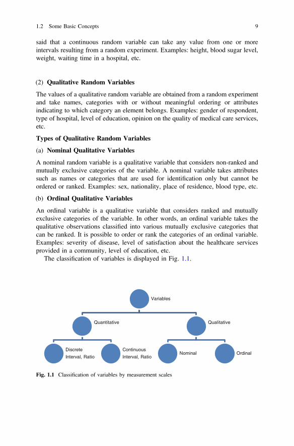
The classification of variables is displayed in Fig. 1.1.
Variables
Quantitative
Discrete
Interval, Ratio
Continuous
Interval, Ratio
Qualitative
Nominal Ordinal
Fig. 1.1 Classification of variables by measurement scales
1.2 Some Basic Concepts 9

1.3 Organizing the Data
After collecting data, the major task is to organize data in such way that will help usto find information which are of interest to a study. Collection of data from aprimary or secondary source is in a format that requires special techniques toarrange the data for answering the questions related to the objectives of a study orexperiment. We need to organize the data from raw form in order to make suitablefor such applications. In this section, some basic techniques for organization of dataare discussed.
1.3.1 Frequency Distribution: Ungrouped
The data are collected on different variables from a well-defined population. Eachvariable can be organized and presented in a suitable form to highlight the mainfeatures of the data. One way to represent the sample data is to find the frequencydistribution. In other words, the data are presented in a form where the character-istics of the original data are presented in a more meaningful way and the basiccharacteristics of the data are self-explanatory.
To organize the data using ungrouped frequency distribution for qualitativevariables or discrete quantitative variables with a small number of distinct valuesare relatively easy computationally. The frequency of a distinct value from a samplerepresents the number of times the value is found in the sample. It means that if avalue occurs 20 times then it is not necessary to write it 20 times rather we may usethe frequency of that value 20, hence, it can be visualized in a more meaningful anduseful way. The relative frequency is defined as the proportion of frequency for avalue in the sample to the sample size. This can be multiplied by 100 to express it inpercentage of the sample size. We can also find the frequency up to a certain valuewhich is called the cumulative frequency.
In ungrouped form, data are displayed for each distinct value of the observations.In case of qualitative variable, the categories of a qualitative variable are summa-rized to display the number of times each category occurs. The number of timeseach category occurs is the frequency of that category and the table is called afrequency distribution table. Each observation is represented by only one categoryin a frequency distribution table such that the total frequency is equal to the samplesize, n. An example below illustrates the construction of an ungrouped frequencydistribution table.
Example 1.1Let us consider hypothetical data on level of education of 16 women in a sample:3, 5, 2, 4, 0, 1, 3, 5, 2, 3, 2, 3, 3, 2, 4, 1 where 0 = no education, 1 = primaryincomplete, 2 = primary complete, 3 = secondary level education, 4 = collegelevel education, and 5 = university level education.
10 1 Basic Concepts, Organizing, and Displaying Data
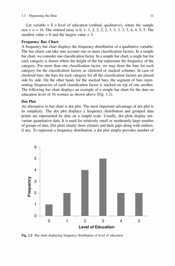
Let variable = X = level of education (ordinal, qualitative), where the samplesize = n = 16. The ordered array is 0, 1, 1, 2, 2, 2, 2, 3, 3, 3, 3, 3, 4, 4, 5, 5. Thesmallest value = 0 and the largest value = 5.
Frequency Bar ChartA frequency bar chart displays the frequency distribution of a qualitative variable.The bar charts can take into account one or more classification factors. In a simplebar chart, we consider one classification factor. In a simple bar chart, a single bar foreach category is drawn where the height of the bar represents the frequency of thecategory. For more than one classification factor, we may draw the bars for eachcategory for the classification factors as clustered or stacked columns. In case ofclustered bars, the bars for each category for all the classification factors are placedside by side. On the other hand, for the stacked bars, the segment of bars repre-senting frequencies of each classification factor is stacked on top of one another.The following bar chart displays an example of a simple bar chart for the data oneducation level of 16 women as shown above (Fig. 1.2).
Dot PlotAn alternative to bar chart is dot plot. The most important advantage of dot plot isits simplicity. The dot plot displays a frequency distribution and grouped datapoints are represented by dots on a simple scale. Usually, dot plots display uni-variate quantitative data. It is used for relatively small or moderately large numberof groups of data. Dot plots clearly show clusters and their gaps along with outliers,if any. To represent a frequency distribution, a dot plot simply provides number of
0
1
2
3
4
5
6
0 1 2 3 4 5
Fre
qu
ency
Level of Education
Fig. 1.2 Bar chart displaying frequency distribution of level of education
1.3 Organizing the Data 11
dots on the vertical axis against the values of the variable on the horizontal axis.Here, the bars are replaced by stacks of dots. From a dot plot, some descriptivemeasures such as mean, median, mode, and range can be obtained easily. It is alsoconvenient to compare two or three frequency distributions using a dot plot.
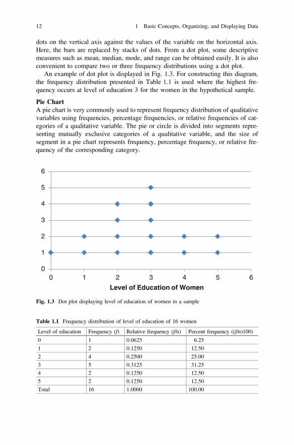
An example of dot plot is displayed in Fig. 1.3. For constructing this diagram,the frequency distribution presented in Table 1.1 is used where the highest fre-quency occurs at level of education 3 for the women in the hypothetical sample.
Pie ChartA pie chart is very commonly used to represent frequency distribution of qualitativevariables using frequencies, percentage frequencies, or relative frequencies of cat-egories of a qualitative variable. The pie or circle is divided into segments repre-senting mutually exclusive categories of a qualitative variable, and the size ofsegment in a pie chart represents frequency, percentage frequency, or relative fre-quency of the corresponding category.
0
1
2
3
4
5
6
0 1 2 3 4 5 6
Level of Education of Women
Fig. 1.3 Dot plot displaying level of education of women in a sample
Table 1.1 Frequency distribution of level of education of 16 women
Level of education Frequency (f) Relative frequency (f/n) Percent frequency ((f/n)100)
0 1 0.0625 6.25
1 2 0.1250 12.50
2 4 0.2500 25.00
3 5 0.3125 31.25
4 2 0.1250 12.50
5 2 0.1250 12.50
Total 16 1.0000 100.00
12 1 Basic Concepts, Organizing, and Displaying Data

A pie chart can be drawn using relative frequencies of a qualitative variable asfollows:
(i) A circle contains 360° which is equivalent to sample size n = total frequencyor 1 in case of relative frequency.
(ii) Compute the relative frequency for each category.(iii) Multiply relative frequency by 360° to find the share of angle size for the
segment corresponding to the category. The total of all the angles corre-sponding to exhaustive and mutually exclusive categories is 360°.
Alternatively, percentage frequency can also be used to draw a pie chart fol-lowing the guidelines stated below.
(i) A circle contains 360° which is equivalent to sample size.(ii) Compute the percentage frequencies for each category which add to 100%
for all the categories combined.(iii) Dividing percentage for each category by 100 provides relative frequency,
and the size of the angle corresponding to a category is obtained by multi-plying the relative frequency by 360°.
The following pie chart displays the level of education of women in a samplewhere the frequency distribution includes 1 in no school, 6 in primary, 5 in sec-ondary, and remaining 4 in college categories. The total sample size is 16. Therelative frequencies are 0.0625, 0.375, 0.3125, and 0.25, respectively, for noschooling, primary, secondary, and college levels, respectively. The angle sizes areobtained by multiplying the relative frequencies by 360° to draw the pie chart asdisplayed below. The sizes of angles for no schooling, primary schooling, sec-ondary schooling, and college level education are 22.5°, 135°, 112.5°, 45°, and 45°,respectively. It can be checked that the total angle size in degrees for the pie chart is22.5 + 135 + 112.5 + 45 + 45 = 360 (Fig. 1.4).
No Schooling
Primary
Secondary
College
Fig. 1.4 Pie chart displaying level of education of women in a sample
1.3 Organizing the Data 13

1.3.2 Grouped Data: The Frequency Distribution
For ungrouped data, the frequency distribution is constructed for distinct values ofcategories or values of the variable. In case of continuous variables, the number ofdistinct values of the variable is too many and it is not meaningful or logical toconstruct the frequency distribution using all the distinct values of the variableobserved in the sample. We know that the continuous random variable takes valuesfrom intervals, and in that case it would be logical to group the set of observationsin intervals called class intervals. These class intervals are contiguous andnonoverlapping and selected suitably such that the sample observations can beplaced in one and, only in one, of the class intervals. These groups are displayed ina frequency distribution table where the frequencies represent the number ofobservations recorded in a group. In grouped data, the choice of class intervalsneeds special attention. If the variable is quantitative and discrete such as size ofhousehold, then intervals such as 1–5, 6–10, 11–15, etc. are nonoverlapping.However, if we consider a continuous variable such as age of individuals admittedto a hospital, then the intervals 0–4, 5–9, 10–14, 15–19, etc. may raise the questionwhat happens if someone reports age between the upper limit of an interval andlower limit of the next interval, for instance, if the reported age is 4 years 6 months.To avoid such ambiguity, if we may consider the intervals 0–5, 5–10, 10–15, etc.,then there is clear overlapping between two consecutive age intervals because theupper limit of an interval is same as the lower limit of the next interval. To addressthis situation, we need to find the true class intervals which ensure continuity of theconsecutive intervals and the values of the observations are considered to benonoverlapping. A simple way to compute the true class interval is summarizedhere: (i) Find the gap between the consecutive class intervals, d = (lower limit of aclass interval − upper limit of the preceding interval); (ii) Divide the gap, d, by 2,i.e., d/2; (iii) Lower limit of the true class interval can be obtained by subtractingd/2 from the lower limit of a class interval; and (iv) Upper limit of the true classinterval can be obtained by adding d/2 to the upper limit of the class interval.
In grouped data, the class intervals are to be constructed in a meaningful waydepending on the nature of data. The number of class intervals should not be toosmall or too large. However, in most of the cases, the number of intervals dependson the purpose of the study. For example, if you conduct a survey to find the agecomposition of the patients admitted to a hospital, then the class intervals may beconsidered in five-yearly intervals such as 0–4, 5–9, 10–14, …, 90–94, where 90–94 is the last interval. Here, the last interval depends on the largest observed value.The five-yearly or ten-yearly age intervals are considered here to keep similaritywith the age compositions available from other sources. However, if we need toconstruct intervals for data from laboratory tests, the intervals need to highlight theranges usually employed for normal, mild complication, severe complication, etc. Ifthese cut-off points are not taken into account, the main purpose of the table is notfulfilled and the table will not provide any meaningful information.
14 1 Basic Concepts, Organizing, and Displaying Data

Let us consider that there are k intervals and the frequencies in those intervals aref1; . . .; fk , then the sum of the frequencies is
Pki¼1 fi ¼ n. Now, we can define the
following terms necessary for constructing a table:
(i) Frequency in the ith class interval: Number of observations in the ith classinterval is fi; i ¼ 1; 2; . . .; k.
(ii) Relative frequency in the ith class interval: Proportion of total observationsin the ith class interval is fi=n, where fi is the frequency in the ith classinterval and n is the sample size, i = 1,2, …, k.
(iii) Percentage relative frequency in the ith class interval: Percentage of totalobservations in the ith class interval is fi=nð Þ�100, where fi is the frequencyin the ith class interval and n is the sample size.
(iv) Cumulative frequency: Number of observations less than or equal to theupper limit of a class interval is the cumulative frequency, usually denoted byFi for the ith class interval. As all the observations are less than the upperlimit of the last class interval, Fk ¼ n. For instance, the cumulative frequencyless than or equal to the upper limit of the first class interval is F1 ¼ f1;similarly, the cumulative frequency less than or equal to the upper limit ofthe second class interval is F2 ¼ f1 þ f2 (alternatively, F2 ¼ F1 þ f2) which isthe sum of frequencies in the first two classes, and the cumulative frequencyless than or equal to the upper limit of the last class interval (or the kth classinterval) is Fk ¼ f1 þ f2 þ � � � þ fk ¼ Fk�1 þ fk which is the sum of fre-quencies in all the classes.
(v) Relative cumulative frequency: Proportion of observations less than or equalto the upper limit of a class interval, which is Fi=n, is called the relativecumulative frequency corresponding to the upper limit of the ith classinterval. As all the observations are less than the upper limit of the last classinterval, the proportion of cumulative frequency in the last class isFk=nð Þ ¼ n=nð Þ ¼ 1.
(vi) Percentage cumulative frequency: Percentage of observations less than orequal to the upper limit of the ith class interval which is Fi=nð Þ�100 is calledthe percentage cumulative frequency corresponding to the upper limit of theith class interval. As all the observations are less than the upper limit of thelast class interval, the corresponding percentage cumulative frequency isFk=nð Þ�100 ¼ n=nð Þ�100 ¼ 100.
Example 1.2The following data represent the weight of 24 women in kilograms taken from arandomly selected enumeration area of Bangladesh Demographic and HealthSurvey 2014.
1.3 Organizing the Data 15

Weight (in kilogram) of 24 women
46.4 53.2 52.8 42 50.8 43
51.9 59.2 55.1 38.9 49.7 43.1
42.2 52.7 49.8 50.7 44.8 49.2
47.7 42.9 52.9 54.1 45.4 49.9
In this example, let us denote the variable X = weight of women (in kg). Thesample size is n = 24. The minimum weight observed in this sample is 38.9 kg.Similarly, the maximum weight is 59.2 kg. The range is the difference between themaximum and the minimum weights which is range = maximum weight − mini-mum weight = 59.2 kg − 38.9 kg = 20.3 kg. The possible class intervals includethe lowest weight in the first and the largest weight in the last interval; we may usethe following intervals of weight: 35.0–39.9, 40.0–44.9, 45.0–49.9, 50.0–54.9, and55.0–59.9. There are 5 class intervals for grouping the weights (in kg) of 24 womenin this example, where the smallest value, 38.9 kg, is included in the first interval,35.0–39.9, and the largest value, 59.2 kg, is included in the last interval, 55.0–59.9.
Table 1.2 displays the construction of frequency distribution table for weights ofwomen using tally marks. Then, dropping the column for tally marks fromTable 1.2, we can display the grouped frequency distribution of the weights of 24women as shown in Table 1.3.
Table 1.2 A frequency distribution table for weights of women for a selected enumeration areafrom BDHS 2014 (n = 24)
Class interval of weights of women (in kg) Tally Frequency (number of women)
35.0–39.9 1
40.0–44.9 6
45.0–49.9 7
50.0–54.9 8
55.0–54.9 2
Table 1.3 A frequencydistribution table for weightsof women for a selectedenumeration area from BDHS2014 (n = 24)
Class interval of weights ofwomen (in kg)
Frequency (number ofwomen)
35.0–39.9 1
40.0–44.9 6
45.0–49.9 7
50.0–54.9 8
55.0–54.9 2
16 1 Basic Concepts, Organizing, and Displaying Data

Mid-Points of Class IntervalsWe can find the mid-point of a class interval as shown below:
mid-point ¼ lower limitþ upper limit2
:
It may be noted here that the mid-point of a class interval is considered as arepetitive or typical value for all observations in that interval.
True Class IntervalsIn a frequency distribution table for a continuous variable, there cannot be any gapbetween two consecutive class intervals as displayed in Table 1.3. It is seen fromTable 1.3 that the first class interval is 35.0–39.9 and the second class interval startsfrom 40.0 and ends at 44.9. Hence, there is a gap, d = 40.0 − 39.9 = 0.1, betweenthe end point of the first interval and the starting point of the second interval. Inother words, there is no continuity between these two points which violates thecondition of continuity necessary for a continuous variable. To overcome thisproblem in constructing the frequency distribution of a continuous variable, let uscompute the true class intervals or class boundaries as follows (Table 1.4):
d = gap between class intervals,d = lower limit − upper limit of the preceding class interval,true upper limit = upper limit + d/2, andtrue lower limit = lower limit − d/2.
The computations mid-points of the first and last intervals are
mid-point of the first interval = (34.95 + 39.95)/2 = 37.45;mid-point of the last interval = (54.95 + 59.95)/2 = 57.45.
It may be noted that (i) mid-point of a class interval can be used to represent allvalues of a class interval approximately, and (ii) there are no gaps between con-secutive true class intervals. It may also be noted that the end point (true upperlimit) of each true class interval equals to the starting point (true lower limit) of thenext true class interval.
Cumulative Frequency Cumulative frequency of the first class interval = F1 ¼ f1.Cumulative frequency of a class interval = frequency + cumulative frequency ofthe preceding class interval. Hence, it can be shown that
Table 1.4 Frequencydistribution of weight ofwomen (in kg) using trueclass intervals
Classinterval
True classinterval
Mid-point Frequency
35.0–39.9 34.95–39.95 37.45 1
40.0–44.9 39.95–44.95 42.45 6
45.0–49.9 44.95–49.95 47.45 7
50.0–54.9 49.95–54.95 52.45 8
55.0–59.9 54.95–59.95 57.45 2
1.3 Organizing the Data 17

F1 ¼ f1;F2 ¼ F1 þ f2;F3 ¼ F2 þ f3;...
Fk ¼ Fk�1 þ fk:
�
Relative Frequency and Percentage Frequency
Relative frequency = frequency/n,Relative frequency of the ith class interval = fiPk
i¼1fi¼ fi
n.
Percentage frequency = Relative frequency � 100%.Percentage frequency of the ith class interval = fiPk
i¼1fi�100% ¼ fi
n�100%.
We can answer different types of questions from the information summarized inTable 1.5. Some examples are shown below using different columns of the table.
Frequency The most frequently responded weight of women belongs to the weightinterval 50.0–54.9 kg and the number of women in this interval is 8.
Cumulative Frequency The number of women having weight less than 50 kg is 14.
Percentage Frequency The percentage of women with weights in the interval50.0–54.9 kg is 33.4% which is one-third of the total number of women in thesample.
Cumulative Percentage Frequency The percentage of women with weight lessthan 55 kg is 58.4%.
Table 1.5 Frequency distribution, relative frequency distribution, cumulative relative frequencydistribution, percentage frequency, and cumulative percentage frequency of weights (in kg) ofwomen
Classinterval
Frequency Cumulativefrequency
Relativefrequency
Cumulativerelativefrequency
Percentagefrequency
Cumulativepercentagefrequency
35.0–39.9 1 1 0.042 0.042 4.2 4.2
40.0–44.9 6 7 0.250 0.292 25.0 29.2
45.0–49.9 7 14 0.292 0.584 29.2 58.4
50.0–54.9 8 22 0.333 0.917 33.3 91.7
55.0–59.9 2 24 0.083 1.000 8.3 100.0
18 1 Basic Concepts, Organizing, and Displaying Data

1.4 Displaying Grouped Frequency Distributions
To display frequency, relative frequency, or percentage frequency distributions, wemay consider one of the following graphs or plots:
(i) The Histogram,(ii) The Frequency Polygon,(iii) Ogive, and(iv) Stem-and-Leaf display.
For illustration of the graphs, the data on weights of 24 women presented in thissection are summarized in Table 1.6. This table is a slightly extended version ofTable 1.4.
HistogramA histogram is constructed for continuous variable. In the X-axis, class boundaries ortrue class intervals and in the Y-axis, the frequencies or relative frequencies are used.The histogram displays the frequency distribution and that is why the underlyingcharacteristics of a frequency distribution are well represented by a histogram. Wecan use the relative frequency to represent the frequency distribution. It is noteworthythat area of rectangle is proportional to the frequency in a histogram. If an interval istwo times of other intervals, then the height for that interval in the Y-axis isheight = (relative frequency/2), in other words, height = (relative frequency/width ofthe interval). The histogram is considered as very useful diagram for self-explanatoryexposition of a data set. There are some disadvantages of histogram: (i) classboundaries are chosen arbitrarily and hence any change in the boundaries may changethe appearance of a histogram quite substantially specially in case of small samples,(ii) the representation of a histogram by rectangular shapes assumes uniformity withineach interval which may not be true in real-life frequency distributions and it dependslargely on the width of an interval, and (iii) the comparison of two or more frequencydistributions by histograms is not a convenient option.
Organizing and Displaying Data using Histogram: Using the data presented inTable 1.5, we can draw the following histogram (Fig. 1.5).
The Frequency PolygonThe frequency polygon is constructed for both continuous and discrete variables.We can use relative frequencies to draw a frequency polygon too. We can plot
Table 1.6 Frequency distribution of weight of women (in kg) using true class intervals
Class interval True class interval Mid-point Frequency Cumulative frequency
35.0–39.9 34.95–39.95 37.45 1 1
40.0–44.9 39.95–44.95 42.45 6 7
45.0–49.9 44.95–49.95 47.45 7 14
50.0–54.9 49.95–54.95 52.45 8 22
55.0–59.9 54.95–59.95 57.45 2 24
1.4 Displaying Grouped Frequency Distributions 19

frequency corresponding to mid-point of each class. Mid-values of class intervalsare plotted along the X-axis and frequencies are plotted at the Y-axis. The latterpoints are then joined by straight lines. The frequency polygon should be broughtdown at each end to the X-axis by joining it to the mid-values of the next outlyinginterval of zero frequency which is called the closed-ended frequency polygon andif the outlying interval of zero frequency is not considered then it is called theopen-ended frequency polygon. The frequency polygon can be used for comparisonby superimposing two or more polygons. Both histogram and frequency polygonsare used to represent frequency distributions.
Example 1.3Let us consider the following hypothetical frequency distribution of the age of 100women (Table 1.7).
Table 1.7 Frequency distribution of age of 100 women
True class interval(age in years)
Frequency(No. of women)
Cumulative Frequency Mid-points
14.5–19.5 8 8 17
19.5–24.5 16 24 22
24.5–29.5 32 56 27
29.5–34.5 28 84 32
34.5–39.5 12 96 37
39.5–44.5 4 100 42
Total n = 100
Width of the interval: W = true upper limit − true lower limit = 19.5 − 14.5 = 5.0
Fig. 1.5 Histogram of weight of women (in kg)
20 1 Basic Concepts, Organizing, and Displaying Data
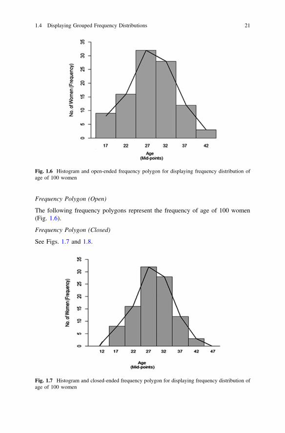
Frequency Polygon (Open)
The following frequency polygons represent the frequency of age of 100 women(Fig. 1.6).
Frequency Polygon (Closed)
See Figs. 1.7 and 1.8.
Fig. 1.6 Histogram and open-ended frequency polygon for displaying frequency distribution ofage of 100 women
Fig. 1.7 Histogram and closed-ended frequency polygon for displaying frequency distribution ofage of 100 women
1.4 Displaying Grouped Frequency Distributions 21
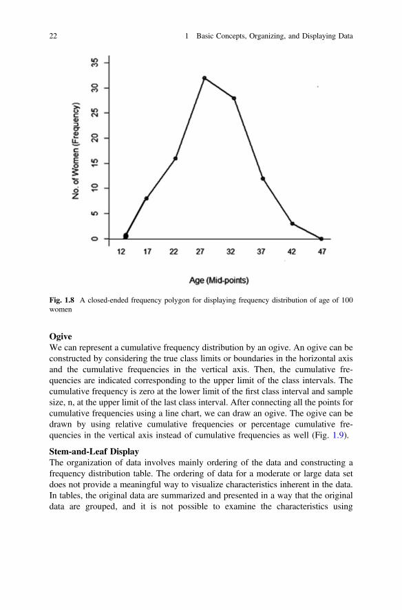
OgiveWe can represent a cumulative frequency distribution by an ogive. An ogive can beconstructed by considering the true class limits or boundaries in the horizontal axisand the cumulative frequencies in the vertical axis. Then, the cumulative fre-quencies are indicated corresponding to the upper limit of the class intervals. Thecumulative frequency is zero at the lower limit of the first class interval and samplesize, n, at the upper limit of the last class interval. After connecting all the points forcumulative frequencies using a line chart, we can draw an ogive. The ogive can bedrawn by using relative cumulative frequencies or percentage cumulative fre-quencies in the vertical axis instead of cumulative frequencies as well (Fig. 1.9).
Stem-and-Leaf DisplayThe organization of data involves mainly ordering of the data and constructing afrequency distribution table. The ordering of data for a moderate or large data setdoes not provide a meaningful way to visualize characteristics inherent in the data.In tables, the original data are summarized and presented in a way that the originaldata are grouped, and it is not possible to examine the characteristics using
Fig. 1.8 A closed-ended frequency polygon for displaying frequency distribution of age of 100women
22 1 Basic Concepts, Organizing, and Displaying Data
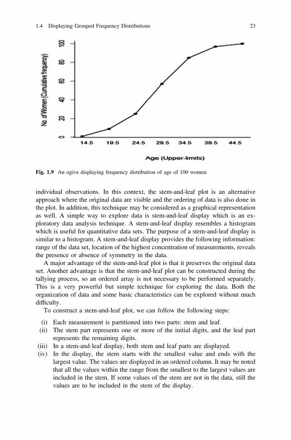
individual observations. In this context, the stem-and-leaf plot is an alternativeapproach where the original data are visible and the ordering of data is also done inthe plot. In addition, this technique may be considered as a graphical representationas well. A simple way to explore data is stem-and-leaf display which is an ex-ploratory data analysis technique. A stem-and-leaf display resembles a histogramwhich is useful for quantitative data sets. The purpose of a stem-and-leaf display issimilar to a histogram. A stem-and-leaf display provides the following information:range of the data set, location of the highest concentration of measurements, revealsthe presence or absence of symmetry in the data.
A major advantage of the stem-and-leaf plot is that it preserves the original dataset. Another advantage is that the stem-and-leaf plot can be constructed during thetallying process, so an ordered array is not necessary to be performed separately.This is a very powerful but simple technique for exploring the data. Both theorganization of data and some basic characteristics can be explored without muchdifficulty.
To construct a stem-and-leaf plot, we can follow the following steps:
(i) Each measurement is partitioned into two parts: stem and leaf.(ii) The stem part represents one or more of the initial digits, and the leaf part
represents the remaining digits.(iii) In a stem-and-leaf display, both stem and leaf parts are displayed.(iv) In the display, the stem starts with the smallest value and ends with the
largest value. The values are displayed in an ordered column. It may be notedthat all the values within the range from the smallest to the largest values areincluded in the stem. If some values of the stem are not in the data, still thevalues are to be included in the stem of the display.
Fig. 1.9 An ogive displaying frequency distribution of age of 100 women
1.4 Displaying Grouped Frequency Distributions 23
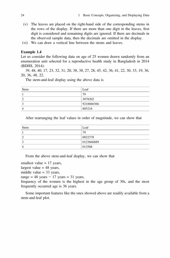
(v) The leaves are placed on the right-hand side of the corresponding stems inthe rows of the display. If there are more than one digit in the leaves, firstdigit is considered and remaining digits are ignored. If there are decimals inthe observed sample data, then the decimals are omitted in the display.
(vi) We can draw a vertical line between the stems and leaves.
Example 1.4Let us consider the following data on age of 25 women drawn randomly from anenumeration unit selected for a reproductive health study in Bangladesh in 2014(BDHS, 2014):
39, 48, 40, 17, 23, 32, 31, 20, 38, 38, 27, 28, 45, 42, 36, 41, 22, 30, 33, 19, 36,20, 36, 48, 22.
The stem-and-leaf display using the above data is
Stem Leaf
1 79
2 3078202
3 9218860366
4 805218
After rearranging the leaf values in order of magnitude, we can show that
Stem Leaf
1 79
2 0022378
3 0123666889
4 012588
From the above stem-and-leaf display, we can show that
smallest value = 17 years,largest value = 48 years,middle value = 33 years,range = 48 years − 17 years = 31 years,frequency of the women is the highest in the age group of 30s, and the mostfrequently occurred age is 36 years.
Some important features like the ones showed above are readily available from astem-and-leaf plot.
24 1 Basic Concepts, Organizing, and Displaying Data

1.5 Designing of Sample Surveys
We have mentioned in the previous sections that data are the raw materials forstatistics. The drawing of a representative sample from the population is the mostimportant part to make the statistical exercises meaningful. In this section, a briefdescription is highlighted for an understanding about the data collection procedureswith introduction to the preliminary concepts necessary for the data collectionprocedures.
1.5.1 Introduction
It is known that the objective of statistics is to make inference about a populationfrom information contained in a sample. Some of the concepts necessary tounderstand the data collection mechanism are described below.
Population: We have already defined population at the beginning of thischapter. In the context of sampling, let us define the population once again. Theentire set of collection of elements about which we wish to make an inference canbe defined as population. In sampling, we may call population as target populationor universe too.
Element: An element is the smallest unit in a sampling on which data arecollected. In other words, measurement on a variable is obtained from an element.
Sampling Unit: Sampling units are elements or group of elements that aredefined clearly, can be identified without any ambiguity, and can be observedconveniently. If the sampling unit is an element, then we may call it samplingelement.
Frame: An exhaustive and nonoverlapping list of all sampling units is called thesampling frame.
Sample: A sample is defined as the collection of sampling units or samplingelements selected for a study with specific objectives from the sampling frame.
1.5.2 Planning a Survey
Each item on the following checklist should be carefully considered in the planningof a survey.
(i) Statement of objectives: It is necessary to state the objectives of the surveyat the planning stage. The stated objectives have to be very clear andprecise. At every stage of survey design and its implementation, the statedobjectives provide the guiding principles.
1.5 Designing of Sample Surveys 25
(ii) Target population: It is necessary to define the population to be sampledand it is called the target population due to its specified domain based on theobjectives of the study as well as its exhaustive coverage of sampling unitsfor selecting the sample. It is important to keep in mind that a sample mustbe selected from the target population such that each unit in the populationcan be assigned with a probability of being selected in the sample.
(iii) Frame: The sampling frame is comprised of the list of all sampling unitsfrom the entire population, nonoverlapping, and exhaustive. It is expectedthat there is close agreement between the target population and list ofsampling units because sampling units are defined using the elements of theentire population.
(iv) Sample design: It is important to choose the design of the sample withspecial attention to number of sampling units/elements and method ofselecting the sampling units/elements from the population in order to fulfillthe stated objectives of a study.
(v) Method of measurement: At the planning stage, it is necessary to decideon the method of measurement. There are several methods of measurementemployed in sampling including personal interviews, telephone interviews,mailed questionnaires, or direct observations.
(vi) Measurement instrument: To collect data from the elements of a survey,we need to specify the necessary measurements and the method of obtainingthe relevant information using appropriate instruments to address theobjectives of the study. This step requires a detailed plan necessary to setthe questions for obtaining the data rigorously. The nonresponse andincorrect response can be minimized by a carefully designed instrument.
(vii) Selection and training of fieldworkers: With a very well-planned design,the success of a sample survey depends to a large extent on the selection,training of fieldworkers, and monitoring the collection of data at the fieldlevel. The fieldworkers are the most important persons responsible forcollecting quality data at the field level. Hence, the implementation of theplans of a survey design heavily depends on the selection and training offieldworkers on questionnaire and measurements for producing quality data.
(viii) Pretest: It is very useful to select a small sample and conduct pretestingprior to implement the survey design. The purpose of a pretest is to findwhether there are deficiencies in the questionnaire or other data collectingmeasurement instrument, training of the fieldworkers, and monitoring ofsurvey design activities. The pretest findings can provide useful feedbacksfor making timely modifications prior to implementation at the field level.
(ix) Organization of fieldwork: To make a large-scale survey successful, theorganization of fieldwork plays a vital role. The management of fieldactivities at the field level involves careful monitoring activities of inter-viewers, coordinators, and data managers with possible backup support.
26 1 Basic Concepts, Organizing, and Displaying Data

(x) Organization of data management: A carefully planned outline of han-dling data at each stage of conducting a survey is an essential step. Inorganizing data, different steps such as code plan, data entry, checking,rechecking, editing, tabulation plan, analysis, etc. are to be planned verycarefully.
(xi) Data analysis: Data analysis is performed on the basis of the objectives ofthe study.
1.5.3 Major Components of Designing a Sample Survey
The major components in designing sample surveys are
(i) sample design,(ii) survey measurements,(iii) survey operations, and(iv) statistical analysis and report writing.
Sample DesignThe core component of designing a sample survey is sample design and dependingon the sample design of a sample survey, other components are planned. Thesample design includes the core tasks of sampling plan and inferential procedure.The selection of sample from the population is designed in the sampling plan of asample survey. The sampling plan provides the methodology of selecting thesampling units and illustrating the selection of elements to be included in thesample from the sampling frame. The sampling plan provides the outline of relatingthe sample to the target population. The inferential procedure provides specific planfor estimation and tests based on the objectives stated for conducting a survey.
Survey MeasurementsThe survey measurements are very crucial that need careful expert opinion andextensive literature review in the light of the underlying objectives of the studybefore making measurements to be employed finally. A pretest can play a vital roleto obtain feedback on whether the measurements are relevant and observable. Themain concern regarding the survey measurements is about addressing the objectivesadequately by analyzing the data obtained from the survey. If there is problem withcore measurements necessary to obtain estimates relevant to the objectives of astudy, the purpose of conducting a sample survey is grossly undermined.
Survey Operations The collection of data is the most important task in a samplesurvey because all the estimates needed to address the stated objectives are obtainedfrom the data that are collected from the field. At this stage, every operation needsto be implemented very carefully because once the data are collected there will beno way to repeat the whole process once again. The quality requirements are to beensured from the beginning and monitored and coordinated with extensive survey
1.5 Designing of Sample Surveys 27

operations strategy for ensuring quality of the data. The steps of survey operationsinclude preparation of the process for data collection, training of the fieldwork teamand management, data collection at the field level, review of field level operationsfor collecting data as an integral part, check for any inconsistency in the mea-surements and necessary remedial steps such as re-interview, repeated attempts toreduce the nonresponse, collection of the measurement instruments followed bydata entry, consistency check, coding process, and storing of data for analysis.
Statistical Analysis and Report WritingAfter the data have been collected at the field level, the processes of coding, editing,and processing for analysis are completed carefully. Once the data are processed,the next step is to use the data for conducting statistical analysis necessary in orderto address the objectives of the sample survey and the findings are presented in afinal report.
1.5.4 Sampling
In a very broad term, we can say that the primary objectives of conducting a samplesurvey are (i) to draw a random sample from the target population and (ii) toestimate the parameters of the target population from the sample.
Probability and Nonprobability SamplingThere are two broad classes of sampling: (i) probability sampling and (ii) non-probability sampling. The definition of a random variable has been introduced inthis chapter, and it is noted that a random variable has an associated probabilitysuch that each value of a random variable has a known and nonzero probability ofbeing selected. In a probability sampling, there is an assigned probability for eachelement of being selected in the sample which is performed by applying the processof randomization. However, in case of a nonprobability sampling, the selection ofelements does not use any randomization and there is no known probabilityof being selected. Only probability sampling can provide the estimated reliability ofwhich can be evaluated. On the other hand, the reliability of an estimate based onnonprobability sampling cannot be evaluated and this weakness restricts a non-probability sampling to generalize the estimates for any target population.
Probability Sampling A variety of probability sampling techniques have beendeveloped to provide efficient practical sample designs:
(i) Simple random sampling,(ii) Stratified sampling,(iii) Systematic sampling,(iv) Cluster sampling,(v) Multistage sampling, etc.
28 1 Basic Concepts, Organizing, and Displaying Data

Simple Random Sampling The simple random sampling is a simple but idealsampling procedure but cannot be applied in many situations particularly in largesurveys. A simple random sampling procedure is performed by drawing a sample ofsize n from a population of size N where each element in the population of sizeN has an equal probability or same chance of being included in the sample. In asimple random sampling, the chance of being selected for every possible sample ofsize n from a population of size N is same. Two types of simple random samplingare (i) simple random sampling with replacement and (ii) simple random samplingwithout replacement. We can use the random number tables for drawing a sampleof size n from a population of size N. A random number table displays a set ofintegers that include all digits (0, 1, …, 9) with equal proportions approximately. Itis noteworthy that there is no observable trend in the patterns of digits included in agenerated random number table (see Appendix A.9).
Stratified Sampling It is important for sample survey to consider a strategy for afixed cost to maximize the amount of information by implementing. It is not alwayspossible to maximize the amount of information by using the simple randomsampling for a fixed cost due to practical reasons and there is a need for alternativesampling procedures. One of the most popular alternatives is the stratified samplingwhich may increase the amount of information for a given cost.
In a simple random sampling procedure, the sample is drawn from a singlepopulation without separating the population elements into separate groups on thebasis of any criteria. Sometimes, it would be cost-effective in terms of sample size ifthe population elements are classified into nonoverlapping groups termed as strata.Then, simple random sampling from each stratum provides the stratified sample.The reasons for choosing a stratified random sampling are as follows:
(i) Stratification is performed usually if there is proven homogeneity withinstrata and there is heterogeneity between strata. In that case, the bound oferror estimation is smaller for sample data from a stratified sampling com-pared to that of a simple random sample of same size.
(ii) Due to construction of strata by taking into account naturally formed groupssuch as rural and urban areas as strata, the cost per element is reduced to alarge extent.
(iii) Sometimes, it is of great importance to obtain estimate for each stratum and astratified random sampling provides the random sample for each stratumfrom which estimates for all the strata can be attained.
Systematic Sampling In a practical sense, both simple random sampling andstratified sampling may involve steps that may pose formidable difficulty forensuring a feasible sample selection process in terms of time and cost. The sys-tematic sampling procedure simplifies the sample selection process and it is usedwidely for practical reasons.
In a systematic sampling, the basic idea is very simple. Instead of sampling eachunit at a time, an appropriate interval of units in the sampling frame is chosen andthe starting point is selected randomly from the first interval of the list and every
1.5 Designing of Sample Surveys 29

other element is selected at equal intervals from the list or frame. This systematicprocedure of selecting the sample with randomization of the element in the firstinterval and selecting the remaining elements at equal intervals is known as thesystematic sampling.
In a link systematic sampling, the first element is selected from the first k ele-ments of the sampling frame and every kth element thereafter is selected from thecomplete list of elements. Often, the systematic sampling is used as an alternative tothe simple random sampling for the reasons listed below:
(i) Selection of elements by simple or stratified random sampling is difficult andmay be subject to error if the sampling frame is not updated or complete. Inthis case, the systematic sampling can provide a sample with less selectionerror at the field level.
(ii) Per unit cost may be reduced to a great extent for a systematic sampling ascompared to simple random sampling.
Cluster Sampling If we consider cluster of elements or collection of elementsinstead of elements, then a cluster sampling can be employed to draw a sample. In acluster sampling, the sampling units are cluster of elements and the clusters areselected using the simple random sampling. For a large sample survey, it is verycostly to prepare the updated sampling frame of elements, and the cost is reducedsubstantially if a cluster of elements is considered as the sampling unit. The cost ofobtaining measurements from elements increases if the selected elements are spreadover at distant locations. On the other hand, the cost is reduced for a clustersampling because the elements form a cluster at the same location. The clustersampling can be used with minimum per unit cost under the following situations:
(i) The sampling frame of elements is either not available or may be very costly toobtain or update but the list of clusters can be obtained and updated easily.
(ii) The distance separating the elements cause increased cost per element insimple or stratified sampling but if the units are clusters then the cost ofobtaining observations from each element reduces substantially.
There is noteworthy difference between construction of strata and clusters. Thestrata are constructed such that there is homogeneity within a stratum but hetero-geneity between strata for the variable being measured from the elements. Inconstructing the cluster, on the other hand, we have to consider just the opposite,heterogeneity within the cluster, and homogeneity between clusters. If the hetero-geneity within and homogeneity between clusters is satisfied, then the clustersampling can produce estimates with very low cost per unit.
Multistage SamplingIt has been stated that cluster sampling is economical under certain circumstances butthe cluster sampling may result in increased variance of the desired estimator for alarge population with large size of clusters. This limitation restricts the use of clustersampling to some extent. A possible remedy is to select only a small number of unitsfrom each cluster rather than collecting data from each element of the selected
30 1 Basic Concepts, Organizing, and Displaying Data

clusters. In that case, we can increase the number of clusters in order to redistributenumber of elements being selected per cluster to a larger number of clusters. In thiscase, two-stage sampling design is conducted. In the first stage, clusters are selectedand at the second stage a specified number of elements are selected from each of theselected clusters. The first stage sampling units are called the primary sampling units(clusters) and the second stage units are called the secondary sampling units (ele-ments). This sampling procedure is known as a two-stage sampling and can be furthergeneralized to multistage sampling for three or higher stages.
Multistage sampling has been extensively used in practice in large-scale surveys.It is noteworthy that the multistage sampling is expected to be
(i) less efficient than single-stage sampling and more efficient than cluster sam-pling from the sampling variability point of view, and
(ii) more efficient than single-stage random sampling and less efficient than clustersampling from the cost and operational point of view.
The main advantage of this sampling procedure is that, at the first stage, theframe of primary sampling units is required, which can be prepared easily. At thesecond stage, the frame of second stage units is required only for the selected PSUs,and so on.
The multistage sampling design is very flexible and allows different selectionprocedures at different stages depending on the requirement of the study. In manypractical situations, the multistage sampling design may be considered as the onlychoice for selecting ultimate sampling units in the context of availability of suitableframe as well as cost per unit.
Design Effect (Deff)With the more complex sampling plans such as multistage sampling, a usefulquantity is the design effect (deff) of the plan. The design effect is described as theratio of the variance of the estimate obtained by employing a more complexsampling technique such as the multistage sampling to the variance of the estimatethat could be obtained from a simple random sampling of the same sample size. Ingeneral, the design effect is used for determining sample size and assessing theefficiency of a more complex sampling technique.
1.5.5 Methods of Data Collection
The major types of data collection methods are:
(i) personal interviews,(ii) telephone interviews,(iii) self-administered questionnaires, and(iv) direct observation.
1.5 Designing of Sample Surveys 31
Personal InterviewsThe personal interviews are conducted on the selected elements with questionnairesconstructed beforehand and the responses are recorded. In most of the cases, therespondents agree to respond if contacted personally. The advantage of personalinterview is obvious, ambiguity in a question can be explained, and reaction of arespondent can be noted on a question. There are some disadvantages too, partic-ularly if the interviewers are not trained adequately or are biased toward certainpotential responses, then that may influence the respondents and will result in biasin the sample data.
Telephone InterviewsTelephone interviews have become a very popular mode of conducting interviews,and the reasons for this popularity are (i) less expensive than personal interviews,(ii) less time is needed because interviewers do not have to travel to the respon-dents, and (ii) can be monitored whether the protocol is maintained or not. Theproblems with telephone interviews cannot be ignored. Some of the limitations are(i) there may be mismatch between sampling frame and list of telephone numbers,(ii) telephone directory may contain numbers do not belong to the potentialrespondents, (iii) there may be unlisted numbers, (iv) telephone interviews must beshort so the number of questions need to be very few, and (v) the nonresponse ratecan be much higher in telephone interviews.
Self-administered QuestionnairesAnother very common mode is use of self-administered questionnaires. In thismethod, the questionnaires are either mailed or distributed using other means toselected individuals of the sample. Using this method, the cost of the survey can beminimized. The major limitation of the self-administered questionnaire method is avery low response rate.
Direct ObservationSometimes, direct observation method is used to collect data if questionnairemethod cannot provide necessary information effectively. If the objective of a studyis to measure change in the behavior, occurrence of an event, physical condition,prevailing situation, etc., then a direct observation may provide necessary data thatcan reflect the objective of a study more appropriately and effectively. The directobservation method can use both the structured and unstructured observationmethods; structured method may provide quantitative data and unstructured methodresults in qualitative data. The use of direct observation methods may be effective ifthe objective of the study is to provide estimates on indicators that do not involveresponses from respondents directly but the observation method can sufficientlyprovide necessary data. This restricts the use of the direct observation method tostudies with only very special needs of such data.
32 1 Basic Concepts, Organizing, and Displaying Data

1.6 Summary
This chapter introduces biostatistics as a discipline that deals with designingstudies, analyzing data, and developing new statistical techniques to address theproblems in the fields of life sciences. This includes collection, organization,summarization, and analysis of data in the fields of biological, health, and medicalsciences including other life sciences. One major objective of a biostatistician is tofind the values that summarize the basic facts from the sample data and to makeinference about the representativeness of the estimates using the sample data tomake inference about the corresponding population characteristics. The basicconcepts are discussed along with examples and sources of data, levels of mea-surement, and types of variables. Various methods of organizing and displayingdata are discussed for both ungrouped and grouped data. The construction of tableis discussed in details. This chapter includes methods of constructing frequency barchart, dot plot, pie chart, histogram, frequency polygon, and ogive. In addition, theconstruction of stem-and-leaf display is discussed in details. All these are illustratedwith examples. As the raw materials of statistics are data, a brief section ondesigning of sample surveys including planning of a survey and major componentsare introduced in order to provide some background about collection of data.
Exercises
1:1 Classify the following variables by the following types: (i) scale of mea-surement, (ii) quantitative or qualitative, (iii) if qualitative, nominal or ordinal,and (iv) if quantitative, discrete, or continuous:
(i) number of patients admitted to a hospital each day,(ii) blood type of children,(iii) age of individuals in a study,(iv) height of individuals in a study,(v) weight of individuals in a study,(vi) duration of stay in emergency care,(vii) level of education,(viii) years of schooling,(ix) gender of respondent,(x) survival status of patient suffered from heart disease,(xi) place of delivery,(xii) current marital status,(xiii) number of children ever born,(xiv) pregnancy resulting in live birth or not,(xv) duration of current pregnancy,(xvi) number of antenatal visits during pregnancy,
1.6 Summary 33
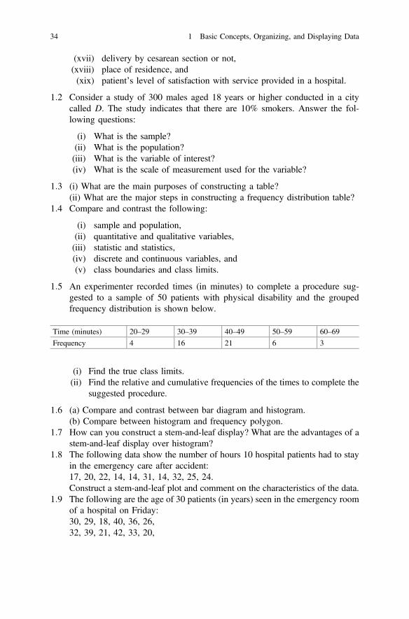
(xvii) delivery by cesarean section or not,(xviii) place of residence, and(xix) patient’s level of satisfaction with service provided in a hospital.
1:2 Consider a study of 300 males aged 18 years or higher conducted in a citycalled D. The study indicates that there are 10% smokers. Answer the fol-lowing questions:
(i) What is the sample?(ii) What is the population?(iii) What is the variable of interest?(iv) What is the scale of measurement used for the variable?
1:3 (i) What are the main purposes of constructing a table?(ii) What are the major steps in constructing a frequency distribution table?
1:4 Compare and contrast the following:
(i) sample and population,(ii) quantitative and qualitative variables,(iii) statistic and statistics,(iv) discrete and continuous variables, and(v) class boundaries and class limits.
1:5 An experimenter recorded times (in minutes) to complete a procedure sug-gested to a sample of 50 patients with physical disability and the groupedfrequency distribution is shown below.
Time (minutes) 20–29 30–39 40–49 50–59 60–69
Frequency 4 16 21 6 3
(i) Find the true class limits.(ii) Find the relative and cumulative frequencies of the times to complete the
suggested procedure.
1:6 (a) Compare and contrast between bar diagram and histogram.(b) Compare between histogram and frequency polygon.
1:7 How can you construct a stem-and-leaf display? What are the advantages of astem-and-leaf display over histogram?
1:8 The following data show the number of hours 10 hospital patients had to stayin the emergency care after accident:17, 20, 22, 14, 14, 31, 14, 32, 25, 24.Construct a stem-and-leaf plot and comment on the characteristics of the data.
1:9 The following are the age of 30 patients (in years) seen in the emergency roomof a hospital on Friday:30, 29, 18, 40, 36, 26,32, 39, 21, 42, 33, 20,
34 1 Basic Concepts, Organizing, and Displaying Data
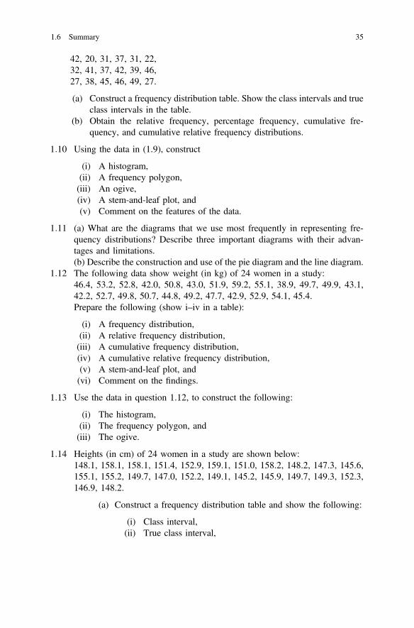
42, 20, 31, 37, 31, 22,32, 41, 37, 42, 39, 46,27, 38, 45, 46, 49, 27.
(a) Construct a frequency distribution table. Show the class intervals and trueclass intervals in the table.
(b) Obtain the relative frequency, percentage frequency, cumulative fre-quency, and cumulative relative frequency distributions.
1:10 Using the data in (1.9), construct
(i) A histogram,(ii) A frequency polygon,(iii) An ogive,(iv) A stem-and-leaf plot, and(v) Comment on the features of the data.
1:11 (a) What are the diagrams that we use most frequently in representing fre-quency distributions? Describe three important diagrams with their advan-tages and limitations.(b) Describe the construction and use of the pie diagram and the line diagram.
1:12 The following data show weight (in kg) of 24 women in a study:46.4, 53.2, 52.8, 42.0, 50.8, 43.0, 51.9, 59.2, 55.1, 38.9, 49.7, 49.9, 43.1,42.2, 52.7, 49.8, 50.7, 44.8, 49.2, 47.7, 42.9, 52.9, 54.1, 45.4.Prepare the following (show i–iv in a table):
(i) A frequency distribution,(ii) A relative frequency distribution,(iii) A cumulative frequency distribution,(iv) A cumulative relative frequency distribution,(v) A stem-and-leaf plot, and(vi) Comment on the findings.
1:13 Use the data in question 1.12, to construct the following:
(i) The histogram,(ii) The frequency polygon, and(iii) The ogive.
1:14 Heights (in cm) of 24 women in a study are shown below:148.1, 158.1, 158.1, 151.4, 152.9, 159.1, 151.0, 158.2, 148.2, 147.3, 145.6,155.1, 155.2, 149.7, 147.0, 152.2, 149.1, 145.2, 145.9, 149.7, 149.3, 152.3,146.9, 148.2.
(a) Construct a frequency distribution table and show the following:
(i) Class interval,(ii) True class interval,
1.6 Summary 35

(iii) Frequency distribution,(iv) Relative frequency distribution,(v) Cumulative frequency distribution,(vi) Relative cumulative frequency distribution,(vii) Construct a stem-and-leaf plot, and(viii) Comment on the main features of the data.
1:15 Use the data in Question 1.14 to construct the following:
(i) The histogram,(ii) The frequency polygon, and(iii) The ogive.
1:16 Fill in the following table on number of hours slept in a study on 100individuals:
Class interval(number ofhours)
Trueclassinterval
Frequency Cumulativefrequency
Relativefrequency
Cumulativerelativefrequency
3.0–4.9 15
5.0–6.9 40 B C
7.0–8.9 30
9.0–10.9 15 A 0.15
Find the following values from the table above:
(a) The value of A is(b) The value of B is(c) The value of C is(d) What percentage of observations is less than 9 h?(e) The true class interval for the first class is(f) The percentage of observations greater than 4.9 h is
1:17 Suppose we have conducted a study on 200 males with age more than20 years living in a city. We want to estimate the average weight for themales of age more than 20 years living in that city. It is found that the averageweight of the men is 76 kg.
(i) What is the variable in this study?(ii) What is the sample size?(iii) (a) What is the scale of the variable?
(b) Is it qualitative or quantitative?(c) If quantitative, discrete or continuous?
36 1 Basic Concepts, Organizing, and Displaying Data

1:18 Classify the following variables by (i) scale of measurement, (ii) quantitativeor qualitative, and (iii) if quantitative, discrete, or continuous:
Variable Scale ofmeasurement
Qualitative/quantitative
Attribute/discrete/continuous
Blood group
Time spent inexerciseDaily
Temperature ofpatients
Quality of service
1.6 Summary 37

Chapter 2Basic Summary Statistics
2.1 Descriptive Statistics
In Chap. 1, we have displayed the techniques of organizing and displaying the data.In this chapter, we introduce the concept of summarization of data by means ofdescriptive measures. A descriptive measure computed from the values of a sampleis called a statistic. A descriptive measure computed from the values of a populationis called a parameter.
As we have mentioned earlier, for the variable of interest, there are N populationvalues, and n sample of values. Let X1;X2; . . .;XN be the population values (ingeneral, they are unknown) of the variable of interest where the populationsize = N and x1; x2; . . .; xn be the sample values (these values are known) where thesample size = n.
A parameter is a measure, quantity, or numerical value obtained from thepopulation values X1;X2; . . .;XN ; and the value of a parameter is generally anunknown but constant value characterizing the population. As the value of aparameter is generally unknown but constant, we are interested in estimating aparameter to understand the characteristic of a population using the sample data.
A statistic is a measure, quantity, or numerical value obtained from the samplevalues x1; x2; . . .; xn and values of statistics can be computed from the sample asfunctions of observations. Since parameters are unknown, statistics are used toapproximate (estimate) parameters.
The necessity of descriptive statistics is quite self-explanatory. In Chap. 1, wehave shown that the data can be organized and presented using figures and tables inorder to display the important features and characteristics contained in data.However, tables and figures may not reveal the underlying characteristics verycomprehensively. For instance, if we want to characterize the data with a singlevalue, it would be very useful not only for communicating to everyone but also formaking comparisons. Let us consider that we are interested in number of c-sectionbirths among the women during their reproductive period in different regions of a
© Springer Nature Singapore Pte Ltd. 2018M. A. Islam and A. Al-Shiha, Foundations of Biostatistics,https://doi.org/10.1007/978-981-10-8627-4_2
39

country. To collect information on this variable, we need to consider women whohave completed their reproductive period. With tables and figures, we can displaytheir frequency distributions. However, to compare tables and figures for differentregions, it would be a very difficult task. In such situations, we need a singlestatistic which contains the salient feature of the data for a region. This single valuecan be a statistic such as arithmetic mean in this case. In case of a qualitativevariable, it could be a proportion. With this single value, we can represent the wholedata set in a meaningful way to represent the corresponding population character-istic and we may compare this value with similar other values at different times orfor different groups or regions conveniently. A single value makes it very conve-nient to represent a whole data set of small, medium, or large size. This would be anideal situation if we could have represented the important features of the data setusing only a single value or a single measure but this may not be the case in reality.Sometimes, we may need more such measures to provide as much insight aspossible.
The descriptive statistics are needed for representing the important features ofdata using only a few measures. These measures are known broadly as descriptivestatistics. Four types of descriptive measures are commonly used for characterizingunderlying features of data:
(i) Measures of central tendency,(ii) Measures of dispersion,(iii) Measures of skewness, and(iv) Measures of kurtosis.
All these measures are used to characterize different features contained in a set ofdata. The first measure, central tendency or location, provides the central valuearound which all other values in the data set are located. In other words, themeasure of central tendency provides the most important representative value of thedata set. The dispersion quantifies or measures the variability in the data wherevariability between values of the data or difference between each value and themeasure of central tendency may reflect how scattered the data are from a centralvalue or what extent in variation among values of the data is there. The thirdmeasure is used to know whether there is symmetry from the central value or thereexists asymmetry from the central value. The fourth measure indicates whether thedata are more concentrated with high peak, low or normal peaks, or frequenciesindicating extent of concentration of values.
2.2 Measures of Central Tendency
The values of a variable often tend to be concentrated around the center of the data.The center of the data can be determined by the measures of central tendency.A measure of central tendency is considered to be a typical (or a representative)
40 2 Basic Summary Statistics

value of the set of data as a whole. The measures of central tendency are sometimesreferred as the measures of location too. The most commonly used measures ofcentral tendency are the mean, the median, and the mode.
2.2.1 Mean
The Population Mean lð ÞIf X1;X2; . . .;XN are the population values, then the population mean is
l ¼ X1 þX2 þ � � � þXN
N¼
PNi¼1 Xi
N:
The population mean l is a parameter. It is usually unknown, and we areinterested to estimate its value.
The Sample Mean �xð ÞIf x1; x2; . . .; xn are the sample values, then the sample mean is
�x ¼ x1 þ x2 þ � � � þ xnn
¼Pn
i¼1 xin
:
It is noteworthy that the sample mean �x is a statistic. It is known and we cancalculate it from the sample. The sample mean �x is used to approximate (estimate)the population mean, l. A more precise way to compute the mean from a frequencydistribution is
�x ¼ f1x1 þ f2x2 þ � � � þ fkxkf1 þ f2 þ � � � þ fk
¼Pk
i¼1 fixin
;
where fi denotes the frequency of distinct sample observation xi; i ¼ 1; . . .; k:
Example 2.1 Let us consider the data on number of children ever born reported by20 women in a sample: 4, 2, 1, 0, 2, 3, 2, 1, 1, 2, 3, 4, 3, 2, 1, 2, 2, 1, 3, 2. Heren = 20. We want to find the average number of children ever born from this sample.
The sample mean is
�x ¼Pn
i¼1 xin
¼ 4þ 2þ 1þ 0þ 2þ 3þ 2þ 1þ 1þ 2þ 3þ 4þ 3þ 2þ 1þ 2þ 2þ 1þ 3þ 220
¼ 4120
¼ 2:05:
Example 2.2 Employing the same data shown above, we can compute the arith-metic mean in a more precise way by using frequencies. We can construct a
2.2 Measures of Central Tendency 41

frequency distribution table from this data to summarize the data first. The fre-quency distribution table is displayed in Table 2.1.
Here, n ¼ P5i¼1 fi ¼ 20 and k = 5. The value of k denotes the number of distinct
values observed for the variable X in the sample. It means that number of times avalue occurs becomes the frequency of that variable. The distinct values observed inthis case are 0, 1, 2, 3, and 4 with frequencies 1, 5, 8, 4, and 2, respectively. Thesample arithmetic can be computed from the above table easily as shown below:
�x ¼Pk
i¼1 fixiPki¼1 fi
¼Pk
i¼1 fixin
¼ 1� 0þ 5� 1þ 8� 2þ 4� 3þ 2� 420
¼ 4120
¼ 2:05:
Advantages and disadvantages of the arithmetic mean
Advantages of the arithmetic mean are
(i) Simplicity: The mean is easily understood and easy to compute.(ii) Uniqueness: There is one and only one mean for a given set of data.(iii) The mean takes into account all values of the data.
Disadvantage
(i) The main disadvantage of the arithmetic mean is that extreme values have aninfluence on the mean. Therefore, the mean may be distorted by extremevalues (Table 2.2).
(ii) The arithmetic mean cannot be used for qualitative data. The arithmetic meancan only be found for quantitative variables.
Example 2.3
Table 2.1 A frequencydistribution table for numberof children ever born of 20women
i Number of children ever born(xi)
Number of women(fi)
1 0 1
2 1 5
3 2 8
4 3 4
5 4 2
Total 20
42 2 Basic Summary Statistics
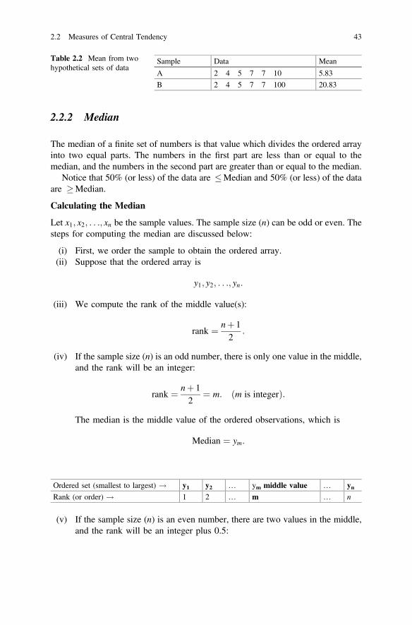
2.2.2 Median
The median of a finite set of numbers is that value which divides the ordered arrayinto two equal parts. The numbers in the first part are less than or equal to themedian, and the numbers in the second part are greater than or equal to the median.
Notice that 50% (or less) of the data are �Median and 50% (or less) of the dataare �Median.
Calculating the Median
Let x1; x2; . . .; xn be the sample values. The sample size (n) can be odd or even. Thesteps for computing the median are discussed below:
(i) First, we order the sample to obtain the ordered array.(ii) Suppose that the ordered array is
y1; y2; . . .; yn:
(iii) We compute the rank of the middle value(s):
rank ¼ nþ 12
:
(iv) If the sample size (n) is an odd number, there is only one value in the middle,and the rank will be an integer:
rank ¼ nþ 12
¼ m: m is integerð Þ:
The median is the middle value of the ordered observations, which is
Median ¼ ym:
Ordered set (smallest to largest) ! y1 y2 … ym middle value … ynRank (or order) ! 1 2 … m … n
(v) If the sample size (n) is an even number, there are two values in the middle,and the rank will be an integer plus 0.5:
Table 2.2 Mean from twohypothetical sets of data
Sample Data Mean
A 2 4 5 7 7 10 5.83
B 2 4 5 7 7 100 20.83
2.2 Measures of Central Tendency 43

rank ¼ nþ 12
¼ mþ 0:5:
Therefore, the ranks of the middle values are (m) and (m + 1).The median is the mean (average) of the two middle values of the ordered
observations:
Median ¼ ym þ ymþ 1
2:
Ordered set y1 y2 … ym ymþ 1 … ynRank (or order) 1 2 m m + 1 … n
Example 2.4 (Odd number) Find themedian for the sample values: 10, 54, 21, 38, 53.
Solutionn = 5 (odd number)
There is only one value in the middle.The rank of the middle value is
rank ¼ nþ 12
¼ 5þ 12
¼ 3: ðm ¼ 3Þ
Ordered set ! 10 21 38 (middle value) 53 54
Rank (or order) ! 1 2 3 (m) 4 5
The median = 38 (unit).
Example 2.5 (Even number) Find the median for the sample values: 10, 35, 41, 16,20, 32.
Solutionn = 6 (even number)
There are two values in the middle. The rank is
rank ¼ nþ 12
¼ 6þ 12
¼ 3:5: ðm ¼ 3Þ
Ordered set ! 10 16 20 (middle value) 32 (middle value) 35 41
Rank (or order) ! 1 2 3 (m) 4 (m + 1) 5 6
The middle values are 20 and 32.The median ¼ 20þ 32
2 ¼ 522 ¼ 26 unitð Þ:
It may be noted here that the unit of the median is the same as the unit of thedata.
44 2 Basic Summary Statistics

Advantages and disadvantages of the medianAdvantages of the median are
(i) Simplicity: The median is easily understood and easy to compute.(ii) Uniqueness: There is only one median for a given set of data.(iii) The median is not as drastically affected by extreme values as is the mean.
An example is illustrated in Table 2.3.Disadvantages of median are as follows:
(i) The median does not take into account all values of the sample after orderingthe data in ascending order.
(ii) In general, the median can only be found for quantitative variables. However,in some cases, the median can be found for ordinal qualitative variables too.
2.2.3 Mode
The mode of a set of values is that value which occurs most frequently (i.e., with thehighest frequency). If all values are different or have the same frequencies, therewill be no mode. A set of data may have more than one mode (Table 2.4).
Example 2.6 It may be noted that the unit of the mode is same as the unit of thedata.
Advantages and disadvantages of the mode
Advantages of the mode are
(i) Simplicity: the mode is easily understood and easy to compute.(ii) The mode is not as drastically affected by extreme values as is the mean
(Table 2.5).(iii) The mode may be found for both quantitative and qualitative variables.
Disadvantages of the mode are as follows:
(i) The mode is not a good measure of location, because it depends on a fewvalues of the data.
(ii) The mode does not take into account all values of the sample.(iii) There might be no mode for a data set.(iv) There might be more than one mode for a data set.
Example 2.7
Table 2.3 Median from twosets of data
Sample Data Median
A 9 4 5 9 2 10 7
B 9 4 5 9 2 100 7
2.2 Measures of Central Tendency 45

2.2.4 Percentiles and Quartiles
The mean, median, and mode are the measures of central tendency. There are othermeasures, percentiles, and quartiles, which do not represent a measure of centraltendency generally (with some exceptions such as median) but represent a measureof position. The measures of position indicate the location of a data set. The medianis a special case of the family of parameters known as position parameters. Thesedescriptive measures are called position parameters because they can be used todesignate certain positions on the horizontal axis when the distribution of a variableis graphed. The position parameters include percentile and quartiles.
Percentile: Given a set of observations x1; x2; . . .; xn, the pth percentile, Pp, p = 0,1, 2,…, 100, is the value of X such that p percent or less of the observations are lessthan Pp and (100 − p) percent or less of the observations are greater than Pp.
The 10th percentile is denoted by P10 where P10 ¼ 10ðnþ 1Þ100
th ordered value:
The 50th percentile is P50 ¼ 50ðnþ 1Þ100
th ordered value ¼ median:
The median is a special case of percentile and it represents the 50th percentile.
Quartile: Given a set of observations x1; x2; . . .; xn, the rth quartile,Qr, r = 1, 2, 3,is the value of X such that ð25� rÞ percent or less of the observations are less thanQr
and [100 − ð25� rÞ] percent or less of the observations are greater than Qr.
Table 2.4 Mode from sevensets of data
Data set Type Mode(s)
26, 25, 25, 34 Quantitative 25
3, 7, 12, 6, 19 Quantitative No mode
3, 3, 7, 7, 12, 12, 6, 6, 19, 19 Quantitative No mode
3, 3, 12, 6, 8, 8 Quantitative 3 and 8
B C A B B B C B B Qualitative B
B C A B A B C A C Qualitative No mode
B C A B B C B C C Qualitative B and C
Table 2.5 Modes from twosets of data with and withoutextreme values
Sample Data Mode
A 7 4 5 7 2 10 7
B 7 4 5 7 2 100 7
46 2 Basic Summary Statistics

For quartiles, we use the following formulas:
Q1 ¼ nþ 14
th ordered observation,
Q2 ¼ 2ðnþ 1Þ4
th ordered observation,
Q3 ¼ 3ðnþ 1Þ4
th ordered observation:
The second quartile is Q2 ¼ 2ðnþ 1Þ4 ¼ nþ 1
2 ¼ median and this is equal to the 50thpercentile.
2.3 Measures of Dispersion
The dispersion of a set of observations refers to the variation contained in the data.A measure of dispersion conveys information regarding the amount of variabilitypresent in a set of data. There are several measures of dispersion, some of which arerange, variance, standard deviation, and coefficient of variation. In addition, somemeasures of dispersion based on percentiles and quartiles are also introduced in thissection. The box-and-whisker plot is a very useful technique to summarize the datawhich is displayed in this section as well.
The variation or dispersion in a set of values refers to how spread out the valuesis from each other. The dispersion is small when the values are close together.There is no dispersion if the values are the same (Figs. 2.1, 2.2 and 2.3; Table 2.6).
Example 2.8 Let us consider the hypothetical data sets of size 5 with same measureof central tendency displayed in Table 2.6, say arithmetic mean in this case:
In this example, if we represent the samples by only measure of central ten-dency, or by arithmetic mean in this case, then all the samples have the same value.In other words, although we observe that the measure of central tendency remains
Fig. 2.1 Displaying median using a dot plot
2.2 Measures of Central Tendency 47

same, the variation contained in each data set, or more specifically, the variation invalues of a data set from its central value are not same at all. This indicates that themeasure of central tendency alone fails to characterize different types of propertiesof data sets. We want to represent the data by a small number of measures, ifpossible by a single value, but sometimes a single value cannot represent the dataadequately or sufficiently. The above example shows one such inadequacy. Themeasure of variation is an additional measure needed to characterize the data inaddition to a measure of central tendency.
Some of the most important measures of dispersion are discussed below.
Fig. 2.2 Figure displaying smaller and larger variations using the same center
Fig. 2.3 Figure displaying small and large variations
Table 2.6 Four sets of datawith same arithmetic mean
Data set 1 8, 9, 10, 11, 12 �x = 10
Data set 2 6, 8, 10, 12, 14 �x = 10
Data set 3 4, 7, 10, 13, 16 �x = 10
Data set 4 2, 6, 10, 14, 18 �x = 10
48 2 Basic Summary Statistics

2.3.1 The Range
The range is the difference between the largest value (Max) and the smallest value(Min):
Range ðRÞ ¼ Max�Min:
Example 2.9 Find the range for the sample values: 26, 25, 35, 27, 29, 29.
Solution
Max ¼ 35
Min ¼ 25
Range ðRÞ = Max�Min ¼ 35� 25 ¼ 10:
The unit of the range is the same as the unit of the data. The usefulness of the rangeis limited. The range is a poor measure of the dispersion because it only takes intoaccount two of the values, maximum and minimum; however, it plays a significantrole in many applications to have a quick view of the dispersion in a data set.
2.3.2 The Variance
The variance is one of the most important measures of dispersion. The variance is ameasure that uses the mean as a point of reference. More precisely, the varianceprovides an average measure of squared difference between each observation andarithmetic mean. The variance of the data is small when the observations are closeto the mean, is large when the observations are spread out from the mean, and iszero (no variation) when all observations have the same value (concentrated at themean). In other words, the variance shows, on an average, how close the values of avariable are to the arithmetic mean.
Deviations of sample values from the sample mean
Let x1; x2; . . .; xn be the sample values, and �x be the sample mean. The deviation ofthe value xi from the sample mean �x is
xi � �x:
The squared deviation is
ðxi � �xÞ2:
2.3 Measures of Dispersion 49

The sum of squared deviations is
Xni¼1
ðxi � �xÞ2:
Figure 2.4 shows the deviations and squared deviations of the values from theirmean.
The Population Variance, r2
Let X1;X2; . . .;XN be the population values. The population variance, r2, is definedby
r2 ¼PN
i¼1 Xi � lð Þ2N
¼ X1 � lð Þ2 þ X2 � lð Þ2 þ � � � þ XN � lð Þ2N
ðunitÞ2
where l ¼PN
i¼1Xi
N is the population mean and N is the population size.It may be noted here that r2 is a parameter because it is obtained from the
population values, it is generally unknown. It is also always true that r2 � 0:
The Sample Variance, s2
Let x1; x2; . . .; xn be the sample values. The sample variance s2 is defined by
s2 ¼Pn
i¼1 ðxi � �xÞ2n
¼ ðx1 � �xÞ2 þðx2 � �xÞ2 þ � � � þ ðxn � �xÞ2n
;
Fig. 2.4 Deviations and squared deviations of sample values from mean
50 2 Basic Summary Statistics

where �x ¼Pn
i¼1xi
n is the sample mean, and n is the sample size. It may be noted herethat the estimate of the population variance can be obtained as
s2 ¼Pn
i¼1 ðxi � �xÞ2n� 1
¼ ðx1 � �xÞ2 þðx2 � �xÞ2 þ � � � þ ðxn � �xÞ2n� 1
:
For our estimate of the variance, we will use this formula to avoid ambiguity inthe subsequent chapters. The underlying reason will be clear in the later chapters onestimation and test of hypothesis.
We can show that the numerator of the variance is
Xn
i¼1ðxi � �xÞ2 ¼
Xn
i¼1x2i � 2�x
Xn
i¼1xi þ
Xn
i¼1�x2
¼Xn
i¼1x2i � 2�xðn�xÞþ n�x2
¼Xn
i¼1x2i � n�x2:
Hence, the sample variance is
s2 ¼Pn
i¼1 x2i � n�x2
n� 1:
Equivalently, we can also express the above for computational convenience as
s2 ¼Pn
i¼1 x2i � n
Pni¼1 xi=n
� �2n� 1
;
which is
s2 ¼Pn
i¼1 x2i �
Pni¼1
xi
� �2
=n
n� 1:
The estimate of the population variance as shown above will be used forinferential purposes in later sections. Hence, we have this expression of the samplevariance subsequently to avoid any ambiguity.
We may note that
(i) s2 is a statistic because it is obtained from the sample values and it is known.(ii) s2 is used to approximate (estimate) r2.(iii) s2 � 0; in other words, the sample variance is nonnegative.(iv) s2 ¼ 0, this happens if all observations have the same value, indicating that
there is no dispersion.
2.3 Measures of Dispersion 51

Using a frequency distribution, the sample variance with denominators n and(n − 1) can be expressed as follows:
s2 ¼Pk
i¼1 fiðxi � xÞ2n
;
and
s2 ¼Pk
i¼1 fiðxi � xÞ2n� 1
:
In both the cases, the arithmetic mean can be expressed as
�x ¼Pk
i¼1 fixiPki¼1 fi
¼Pk
i¼1 fixin
:
Example 2.10 We want to compute the sample variance of the following samplevalues: 10, 21, 33, 53, 54.
Solutionn = 5
�x ¼Pn
i¼1 xin
¼P5
i¼1 xi5
¼ 10þ 21þ 33þ 53þ 545
¼ 1715
¼ 34:2
s2 ¼Pn
i¼1 xi � �xð Þ2n� 1
¼P5
i¼1 xi � 34:2ð Þ25� 1
:
s2 ¼ 10� 34:2ð Þ2 þ 21� 34:2ð Þ2 þ 33� 34:2ð Þ2 þ 53� 34:2ð Þ2 þ 54� 34:2ð Þ24
¼ 1506:84
¼ 376:7:
Another method for calculating sample variance:
xi xi � xð Þ ¼ xi � 34:2ð Þ xi � xð Þ2 ¼ xi � 34:2ð Þ210 −24.2 585.64
21 −13.2 174.24
33 −1.2 1.44
53 18.8 353.44
54 19.8 392.04P5i¼1 xi ¼ 171
P5i¼1 xi � �xð Þ ¼ 0
Pxi � �xð Þ2¼ 1506:8
52 2 Basic Summary Statistics

x ¼P5
i¼1 xi5
¼¼ 1715
¼ 34:2 and s2 ¼ 1506:84
¼¼ 376:7:
Using the alternative methods, we can compute the sample variance for the samedata as shown below:
s2 ¼Pn
i¼1 x2i � n�x2
n� 1
where
X5
i¼1x2i ¼ 102 þ 212 þ 332 þ 532 þ 542 ¼ 100þ 441þ 1089þ 2809þ 2916 ¼ 7355;
n�x2 ¼ 5� ð34:2Þ2 ¼ 5� 1169:64 ¼ 5848:20; and
s2 ¼P5
i¼1 x2i � nx2
5� 1¼ 7355� 5848:20
4¼ 1506:80
4¼ 376:70:
Similarly,
s2 ¼Pn
i¼1 x2i � ðPn
i¼1 xiÞ2=nn� 1
;
where
X5
i¼1x2i ¼ 102 þ 212 þ 332 þ 532 þ 542 ¼ 100þ 441þ 01089þ 2809þ 2916 ¼ 7355;X5
i¼1xi
� �2=5 ¼ ð171Þ2=5 ¼ 29241
5¼ 5848:20; and
s2 ¼P5
i¼1 x2i � ðP5
i¼1 xiÞ2=55� 1
¼ 7355� 5848:204
¼ 1506:804
¼ 376:70:
2.3.3 Standard Deviation
The variance represents squared units, and therefore is not appropriate measure ofdispersion when we wish to express the concept of dispersion in terms of theoriginal unit. The standard deviation is another measure of dispersion. The standarddeviation is the positive square root of the variance and is expressed in the originalunit of the data.
(i) Population standard deviation is r ¼ffiffiffiffiffir2
p:
(ii) Sample standard deviation is s ¼ffiffiffiffis2
p;
2.3 Measures of Dispersion 53

s ¼ffiffiffiffiffiffiffiffiffiffiffiffiffiffiffiffiffiffiffiffiffiffiffiffiffiffiffiffiffiPn
i¼1 ðxi � xÞ 2n� 1
s:
Example 2.11 For the previous example, the sample standard deviation is
s ¼ffiffiffiffis2
p¼
ffiffiffiffiffiffiffiffiffiffiffi376:7
p¼ 19:41:
2.3.4 Coefficient of Variation (C.V.)
Although the variance and the standard deviation are useful measures of variationof the values of a single variable for a single population, sometimes we need tocompare the variation of two variables. In that case, we cannot use the variance orthe standard deviation directly, because (i) the variables might have different unitsand (ii) the variables might have different means. For comparison, we need ameasure of the relative variation that does not depend on either the units or on thevalues of means. This measure is called the coefficient of variation (C.V.).
The coefficient of variation is defined by
C:V: ¼ s�x� 100%:
It is clearly evident that the C.V. is free of unit and the standard deviation isdivided by the corresponding arithmetic mean to make it comparable for differentmeans.
To compare the variability of two sets of data (i.e., to determine which set ismore variable), we need to calculate the following quantities:
Data set Mean Standard deviation C.V.
1 �x1 s1 C.V:1 ¼ s1�x1100%
2 �x2 s2 C.V.2 ¼ s2�x2100%
The data set with the larger value of C.V. has larger variation which is expressedin percentage. The relative variability of the data set 1 is larger than the relativevariability of the data set 2 if C.V.1 > C.V.2 and vice versa.
Example 2.12 Suppose we have two data sets from two samples:Data set 1: Let us consider that from the data in sample 1, the mean and the standarddeviation are �x1 ¼ 66 kg and s1 ¼ 4.5 kg, respectively. Hence, the coefficient ofvariation is
54 2 Basic Summary Statistics

C.V.1 ¼ 4:566
� 100% ¼ 6:8%:
Data set 2: The mean and the standard deviation from the second sample are x2 ¼36 kg and s2 ¼ 4.5 kg, respectively. The coefficient of variation for this data set is
C.V.2 ¼ 4:536
� 100% ¼ 12:5%:
Since C.V.2 [C.V.1, the relative variability of the data set 2 is larger than therelative variability of the data set 1.
If we use the standard deviation to compare the variability of the two data sets,we will wrongly conclude that the two data sets have the same variability becausethe standard deviation of both sets is 4.5 kg.
2.3.5 Some Properties of �x; s; s2
Let the sample values are x1; x2; . . .; xn and let a and b are constants. Then, we cansummarize the impact of the shift in origin and scale in the data on the variance andstandard deviation as follows:
Case Sample data Samplemean
Sample standarddeviation
Samplevariance
1 x1; . . .; xn �x s s2
2 ax1; . . .; axn a�x aj js a2s2
3 x1 þ b; . . .; xn þ b �xþ b s s2
4 ax1 þ b; . . .; axn þ b a�xþ b aj js a2s2
Case 1 Case 1 represents the data without any change in the origin or scale.Hence, the mean, the standard deviation, and the variance represent the measuresunaffected.
Example 2.13 Let us consider a hypothetical data set of size 5 as follows:
x1 ¼ 3; x2 ¼ 1; x3 ¼ 4; x4 ¼ 2; x5 ¼ 1:
Using these data, we obtain the following measures of central tendency andvariation
�x ¼ 2:2;
s ¼ 1:3038;
s2 ¼ 1:7:
2.3 Measures of Dispersion 55
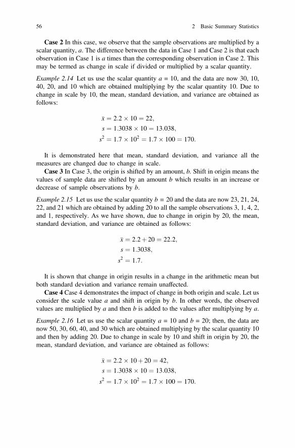
Case 2 In this case, we observe that the sample observations are multiplied by ascalar quantity, a. The difference between the data in Case 1 and Case 2 is that eachobservation in Case 1 is a times than the corresponding observation in Case 2. Thismay be termed as change in scale if divided or multiplied by a scalar quantity.
Example 2.14 Let us use the scalar quantity a = 10, and the data are now 30, 10,40, 20, and 10 which are obtained multiplying by the scalar quantity 10. Due tochange in scale by 10, the mean, standard deviation, and variance are obtained asfollows:
�x ¼ 2:2� 10 ¼ 22;
s ¼ 1:3038� 10 ¼ 13:038;
s2 ¼ 1:7� 102 ¼ 1:7� 100 ¼ 170:
It is demonstrated here that mean, standard deviation, and variance all themeasures are changed due to change in scale.
Case 3 In Case 3, the origin is shifted by an amount, b. Shift in origin means thevalues of sample data are shifted by an amount b which results in an increase ordecrease of sample observations by b.
Example 2.15 Let us use the scalar quantity b = 20 and the data are now 23, 21, 24,22, and 21 which are obtained by adding 20 to all the sample observations 3, 1, 4, 2,and 1, respectively. As we have shown, due to change in origin by 20, the mean,standard deviation, and variance are obtained as follows:
�x ¼ 2:2þ 20 ¼ 22:2;
s ¼ 1:3038;
s2 ¼ 1:7:
It is shown that change in origin results in a change in the arithmetic mean butboth standard deviation and variance remain unaffected.
Case 4 Case 4 demonstrates the impact of change in both origin and scale. Let usconsider the scale value a and shift in origin by b. In other words, the observedvalues are multiplied by a and then b is added to the values after multiplying by a.
Example 2.16 Let us use the scalar quantity a = 10 and b = 20; then, the data arenow 50, 30, 60, 40, and 30 which are obtained multiplying by the scalar quantity 10and then by adding 20. Due to change in scale by 10 and shift in origin by 20, themean, standard deviation, and variance are obtained as follows:
�x ¼ 2:2� 10þ 20 ¼ 42;
s ¼ 1:3038� 10 ¼ 13:038;
s2 ¼ 1:7� 102 ¼ 1:7� 100 ¼ 170:
56 2 Basic Summary Statistics

It is demonstrated here that mean, standard deviation, and variance all thesemeasures are changed due to change in scale and shift in origin. In this case, thearithmetic mean is affected by both change in scale and shift in origin but standarddeviation and variance are affected due to change in scale only.
A more detailed example is shown below.
Example 2.17 Let us consider a sample of size 5 as follows: 5, 3, 2, 4, 1. Let a = 3and b = 5. Then, the mean, variance, and standard deviations from the original datax1 ¼ 5, x2 ¼ 3, x3 ¼ 2, x4 ¼ 4, and x5 ¼ 1 are
�x ¼P5
i¼1 xi5
¼ 5þ 3þ 2þ 4þ 15
¼ 155
¼ 3;
s2 ¼P5
i¼1 x2i � ðP5
i¼1 xiÞ2=55� 1
¼ 52 þ 32 þ 22 þ 42 þ 12 � ð15Þ2=54
¼ 55� 454
¼ 104
¼ 2:5;
s ¼ffiffiffiffiffiffiffi2:5
p¼ 1:5811:
Let us consider that the scale is changed by a, then the new data set isax1; ax2; . . .; axn. Here, a = 3 and n = 5; hence, the mean, the variance, and thestandard deviation are
mean = a�x ¼ 3� 3 ¼ 9;
variance ¼ a2s2 ¼ 9� 2:5 ¼ 22:5 ¼ 2:5; and
standard deviation ¼ aj js ¼ 3j jffiffiffiffiffiffiffi2:5
p¼ 3� 1:5811 ¼ 4:7433:
This shows that change in the scale changes both the mean and the variancewhich implies change in the standard deviation as well.
If we shift the origin by 5 such that the new data set is x1 þ b; x2 þ 5; . . .; xn þ 5,then the mean, variance, and standard deviation are
mean ¼ �xþ b ¼ 3þ 5 ¼ 8;
variance ¼ s2 ¼ 2:5; and
standard deviation ¼ s ¼ffiffiffiffiffiffiffi2:5
p¼ 1:5811:
It is clearly observed that if the origin is shifted by any value, then the mean isshifted too but the variance and standard deviation remain unchanged. In otherwords, the mean is affected by a shift in the origin but variance and standarddeviation are not affected.
Similarly, if we change both the scale and origin such that the new data set isax1 þ b; ax2 þ b; . . .; axn þ b, then we obtain the following:
2.3 Measures of Dispersion 57
mean ¼ a�xþ b ¼ 3� 3þ 5 ¼ 9þ 5 ¼ 14;
variance ¼ a2s2 ¼ 9� 2:5 ¼ 22:5 ¼ 2; 5; and
standard deviation ¼ aj js ¼ 3j jffiffiffiffiffiffiffi2:5
p¼ 3� 1:5811 ¼ 4:7433:
This shows that if we consider changes in both scale and origin, then the mean isaffected by both but the variance and standard deviation need to be adjusted foronly the quantity of the change in scale only. In other words, the measure of centraltendency, mean, depends on both the scale and origin but the measures of dis-persion, variance, and standard deviation are independent of change in the originbut depend on the change in the scale.
2.3.6 Interquartile Range
A disadvantage of the range is that it is computed using the two extreme values ofthe sample data, the smallest and the largest values. If the data contain extremeoutlier values, then the range is affected by those outliers. To overcome this limi-tation of the range, an alternative measure called the interquartile range can be used.The interquartile range is computed by taking the difference between the thirdquartile and the first quartile. The interquartile range provides a more meaningfulmeasure that represents the range of the middle 50% of the data. The interquartilerange is defined as
IQR ¼ Q3 � Q1;
where Q3 is the third quartile and Q1 is the first quartile. As the extreme values arenot considered, the IQR is a more robust measure of variation in the data and is notaffected by outliers. The semi-interquartile range is defined as
ðQ3 � Q1Þ=2:
2.3.7 Box-and-Whisker Plot
We know that a measure of central tendency or location is a value around whichother values are clustered. The variation or spread in the data from the central valueis usually measured by a measure of dispersion. In addition, we want to knowwhether the data are symmetric or not. The box-and-whisker plot displays all thesein a simple plot where the box contains features included in the middle 50% of the
58 2 Basic Summary Statistics
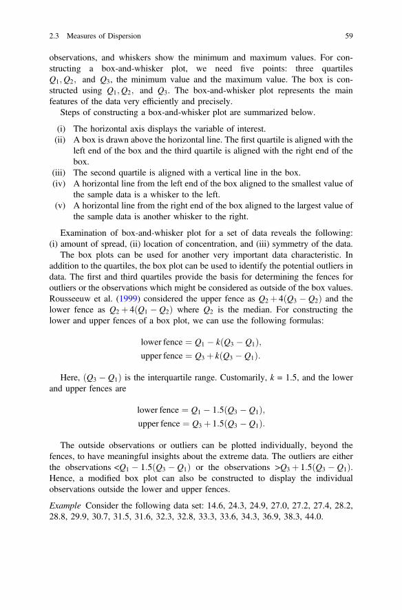
observations, and whiskers show the minimum and maximum values. For con-structing a box-and-whisker plot, we need five points: three quartilesQ1;Q2; and Q3, the minimum value and the maximum value. The box is con-structed using Q1;Q2; and Q3. The box-and-whisker plot represents the mainfeatures of the data very efficiently and precisely.
Steps of constructing a box-and-whisker plot are summarized below.
(i) The horizontal axis displays the variable of interest.(ii) A box is drawn above the horizontal line. The first quartile is aligned with the
left end of the box and the third quartile is aligned with the right end of thebox.
(iii) The second quartile is aligned with a vertical line in the box.(iv) A horizontal line from the left end of the box aligned to the smallest value of
the sample data is a whisker to the left.(v) A horizontal line from the right end of the box aligned to the largest value of
the sample data is another whisker to the right.
Examination of box-and-whisker plot for a set of data reveals the following:(i) amount of spread, (ii) location of concentration, and (iii) symmetry of the data.
The box plots can be used for another very important data characteristic. Inaddition to the quartiles, the box plot can be used to identify the potential outliers indata. The first and third quartiles provide the basis for determining the fences foroutliers or the observations which might be considered as outside of the box values.Rousseeuw et al. (1999) considered the upper fence as Q2 þ 4ðQ3 � Q2Þ and thelower fence as Q2 þ 4ðQ1 � Q2Þ where Q2 is the median. For constructing thelower and upper fences of a box plot, we can use the following formulas:
lower fence ¼ Q1 � kðQ3 � Q1Þ;upper fence ¼ Q3 þ kðQ3 � Q1Þ:
Here, ðQ3 � Q1Þ is the interquartile range. Customarily, k = 1.5, and the lowerand upper fences are
lower fence ¼ Q1 � 1:5ðQ3 � Q1Þ;upper fence ¼ Q3 þ 1:5ðQ3 � Q1Þ:
The outside observations or outliers can be plotted individually, beyond thefences, to have meaningful insights about the extreme data. The outliers are eitherthe observations <Q1 � 1:5ðQ3 � Q1Þ or the observations >Q3 þ 1:5ðQ3 � Q1Þ.Hence, a modified box plot can also be constructed to display the individualobservations outside the lower and upper fences.
Example Consider the following data set: 14.6, 24.3, 24.9, 27.0, 27.2, 27.4, 28.2,28.8, 29.9, 30.7, 31.5, 31.6, 32.3, 32.8, 33.3, 33.6, 34.3, 36.9, 38.3, 44.0.
2.3 Measures of Dispersion 59

Here, n = 20.
Q1 ¼ nþ 14
th ordered observation ¼ 20þ 14
¼ 5:25th ordered observation
¼ 5th ordered observationþð0:25Þð27:4� 27:2Þ ¼ 27:2þð0:25Þð0:2Þ ¼ 27:25
Q2 ¼ 2ðnþ 1Þ4
th ordered observation ¼ 20þ 12
¼ 10:5th ordered observation
¼ 10th ordered observationþð0:5Þð31:5� 30:7Þ¼ 30:7þð0:5Þð31:5�30:7Þ ¼ 31:1
Q3 ¼ 3ðnþ 1Þ4
th ordered observation ¼ 3ð20þ 1Þ4
¼ 15:75th ordered observation
¼ 15th ordered observationþð0:75Þð33:6� 33:3Þ¼ 33:3þð0:75Þð33:6�33:3Þ ¼ 33:525
IQR ¼ 33:525� 27:25 ¼ 6:275
Range ¼ 44:0� 14:6 ¼ 29:4
Ratio of IQR to Range (% ) ¼ 6:27529:4
� 100 ¼ 21% of range:
Using the data shown in this example, we can construct the box-and-whiskerplot or box plot. The traditional box plot is based on five points, Q1;Q2; and Q3 fordrawing the box and minimum and maximum values for the whiskers as shown inFig. 2.5.
The second box plot shows the box plot where in addition to the box usingQ1;Q2; and Q3, the lower and upper fences are also shown. The lower and upperfences are
Fig. 2.5 Box-and-whisker plot
60 2 Basic Summary Statistics

lower fence ¼ Q1 � 1:5 Q3 � Q1ð Þ¼ 27:25� 1:5� IQR
¼ 27:25� 1:5� 6:275
¼ 17:8375
and
upper fence ¼ Q3 þ kðQ3 � Q1Þ¼ 33:525þ 1:5� IQR
¼ 33:525þ 1:5� 6:275
¼ 42:9375:
We can find the outliers from the observations either the observations<Q1 � 1:5ðQ3 � Q1Þ or the observations >Q3 þ 1:5ðQ3 � Q1Þ. It is observed thatfollowing this rule for detecting the outliers, there are two outliers in the sample data:one is less than the lower fence or outside the lower fence, 14.6, and the other value isgreater than the upper fence or outside the upper fence, 44.0.
The results from sample data used for constructing Fig. 2.6 are sample size: 20,median: 31.1, minimum: 14.6, maximum: 44.0, first quartile: 27.25, third quartile:33.525, interquartile range: 6.275, lower fence = 17.8375, upper fence = 42.9375,and outliers: 14.6, 44.0, as shown in Fig. 2.6.
2.4 Moments of a Distribution
The moments are used to summarize the characteristics of data. These are de-scriptive statistics if calculated from sample that can be used to explore charac-teristics of data such as central tendency, dispersion, skewness, and kurtosis. Themeasures of skewness and kurtosis are shape characteristics of the data which willbe discussed in subsequent sections. We can define both the population and samplemoments but for the sake of simplicity only sample moments are defined in thissection. The moments can be classified as (i) the raw moments, (ii) the momentsabout any arbitrary value a, and (iii) the moments about mean or the centralmoments.
Let x1; x2; . . .; xn be the n values assumed by the variable, X, then the quantity
m0r ¼
Pni¼1 x
ri
n
is called the rth raw sample moment of the variable, X.
2.3 Measures of Dispersion 61

The rth sample moment about any value a, also denoted by m0r, is defined as
m0r ¼
Pni¼1 ðxi � aÞr
n:
The rth central moment about mean or the rth moment about the mean is defined as
mr ¼Pn
i¼1 ðxi � �xÞrn
:
Fig. 2.6 Box-and-whiskerplot displaying outliers fromthe sample data; sample size:20, median: 31.1, minimum:14.6, maximum: 44.0, firstquartile: 27.25, third quartile:33.525, interquartile range:6.275, and outliers: 14.6, 44.0
62 2 Basic Summary Statistics
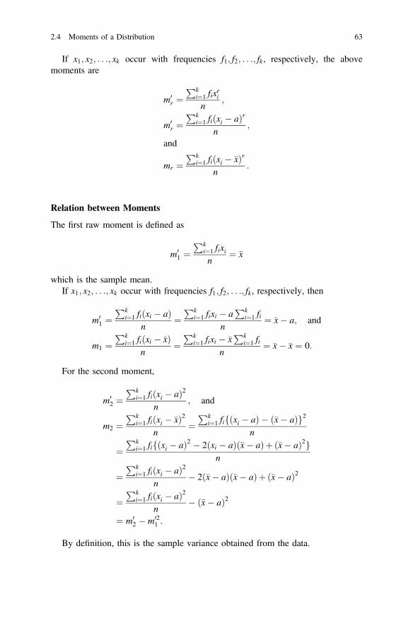
If x1; x2; . . .; xk occur with frequencies f1; f2; . . .; fk , respectively, the abovemoments are
m0r ¼
Pki¼1 fix
ri
n;
m0r ¼
Pki¼1 fiðxi � aÞr
n;
and
mr ¼Pk
i¼1 fiðxi � �xÞrn
:
Relation between Moments
The first raw moment is defined as
m01 ¼
Pki¼1 fixin
¼ �x
which is the sample mean.If x1; x2; . . .; xk occur with frequencies f1; f2; . . .; fk , respectively, then
m01 ¼
Pki¼1 fiðxi � aÞ
n¼
Pki¼1 fixi � a
Pki¼1 fi
n¼ �x� a; and
m1 ¼Pk
i¼1 fiðxi � �xÞn
¼Pk
i¼1 fixi � �xPk
i¼1 fin
¼ �x� �x ¼ 0:
For the second moment,
m02 ¼
Pki¼1 fiðxi � aÞ2
n; and
m2 ¼Pk
i¼1 fiðxi � �xÞ2n
¼Pk
i¼1 fifðxi � aÞ � ð�x� aÞg2n
¼Pk
i¼1 fifðxi � aÞ2 � 2ðxi � aÞð�x� aÞþ ð�x� aÞ2gn
¼Pk
i¼1 fiðxi � aÞ2n
� 2ð�x� aÞð�x� aÞþ ð�x� aÞ2
¼Pk
i¼1 fiðxi � aÞ2n
� ð�x� aÞ2
¼ m02 � m02
1 :
By definition, this is the sample variance obtained from the data.
2.4 Moments of a Distribution 63

Similarly, it can also be shown that
m3 ¼ m03 � 3m0
2m01 þ 2m03
1 ; and
m4 ¼ m04 � 4m0
3m01 þ 6m0
2m021 � 3m04
1 :
Example 2.19 Let us consider the following data from a sample:x1 ¼ 2; x2 ¼ 1; x3 ¼ 4; x4 ¼ 0; x5 ¼ 2, n = 5.
The sample raw moments are
m01 ¼
2þ 1þ 4þ 0þ 25
¼ 95¼ 1:8
m02 ¼
22 þ 12 þ 42 þ 02 þ 22
5¼ 25
5¼ 5
m03 ¼
23 þ 13 þ 43 þ 03 þ 23
5¼ 81
5¼ 16:2
m04 ¼
24 þ 14 þ 44 þ 04 þ 24
5¼ 289
5¼ 57:8:
Using the relationships between raw and central moments, we can compute thecentral sample moments as follows:
m2 ¼ m02 � m02
1 ¼ 5� ð1:8Þ2 ¼ 1:76
m3 ¼ m03 � 3m0
2m01 þ 2m03
1 ¼ 16:2� 3� 5� 1:8þ 2� ð1:8Þ3¼ 0:864;
m4 ¼ m04 � 4m0
3m01 þ 6m0
2m021 � 3m04
1 ¼ 57:8� 4� 16:2� 1:8þ 6� 5� ð1:8Þ2 � 3� ð1:8Þ4¼ 6:8672:
2.5 Skewness
Skewness is the degree of asymmetry or departure of symmetry of a distribution. Ina skew distribution, the mean tends to lie on the same side of the mode as the longertail. In a symmetric distribution, the mean, the mode, and the median coincide.Some commonly used measures of skewness are discussed as shown in Fig. 2.7.
64 2 Basic Summary Statistics

Pearson’sMeasure
skewness ¼ (mean-mode)standard deviation
¼ 0 for symmetry,
[ 0 for positively skewed distribution,
\0 for negatively skewed distribution.
Alternatively,
skewness ¼ 3(mean-median)standard deviation
¼ 0 for symmetry,
[ 0 for positively skewed distribution,
\0, for negatively skewed distribution.
Bowley’sMeasure
skewness ¼ ðQ3 � Q2Þ � ðQ2 � Q1ÞðQ3 � Q1Þ
ðQ3 � Q2Þ ¼ ðQ2 � Q1Þ for symmetry,
ðQ3 � Q2Þ[ ðQ2 � Q1Þ for positively skewed distribution,
ðQ3 � Q2Þ\ðQ2 � Q1Þ for negatively skewed distribution.
Example 2.20 Consider the following data set: 14.6, 24.3, 24.9, 27.0, 27.2, 27.4,28.2, 28.8, 29.9, 30.7, 31.5, 31.6, 32.3, 32.8, 33.3, 33.6, 34.3, 36.9, 38.3, 44.0.
Here, n = 20. �x ¼ 30:58: There is no mode. The sample variance, s2 ¼ 36:3417and the sample standard deviation, s ¼ 6:0284:
Fig. 2.7 Symmetric, negatively skewed, and positively skewed curves
2.5 Skewness 65
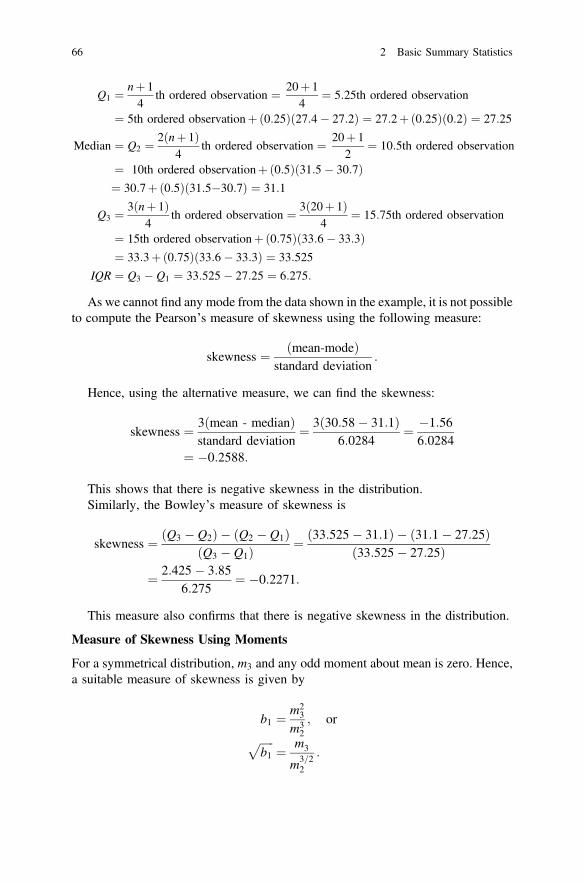
Q1 ¼ nþ 14
th ordered observation ¼ 20þ 14
¼ 5:25th ordered observation
¼ 5th ordered observationþð0:25Þð27:4� 27:2Þ ¼ 27:2þð0:25Þð0:2Þ ¼ 27:25
Median ¼ Q2 ¼ 2ðnþ 1Þ4
th ordered observation ¼ 20þ 12
¼ 10:5th ordered observation
¼ 10th ordered observationþð0:5Þð31:5� 30:7Þ¼ 30:7þð0:5Þð31:5�30:7Þ ¼ 31:1
Q3 ¼ 3ðnþ 1Þ4
th ordered observation ¼ 3ð20þ 1Þ4
¼ 15:75th ordered observation
¼ 15th ordered observationþð0:75Þð33:6� 33:3Þ¼ 33:3þð0:75Þð33:6� 33:3Þ ¼ 33:525
IQR ¼ Q3 � Q1 ¼ 33:525� 27:25 ¼ 6:275:
As we cannot find any mode from the data shown in the example, it is not possibleto compute the Pearson’s measure of skewness using the following measure:
skewness ¼ ðmean-modeÞstandard deviation
:
Hence, using the alternative measure, we can find the skewness:
skewness ¼ 3ðmean - medianÞstandard deviation
¼ 3ð30:58� 31:1Þ6:0284
¼ �1:566:0284
¼ �0:2588:
This shows that there is negative skewness in the distribution.Similarly, the Bowley’s measure of skewness is
skewness ¼ ðQ3 � Q2Þ � ðQ2 � Q1ÞðQ3 � Q1Þ ¼ ð33:525� 31:1Þ � ð31:1� 27:25Þ
ð33:525� 27:25Þ¼ 2:425� 3:85
6:275¼ �0:2271:
This measure also confirms that there is negative skewness in the distribution.
Measure of Skewness Using Moments
For a symmetrical distribution, m3 and any odd moment about mean is zero. Hence,a suitable measure of skewness is given by
b1 ¼ m23
m32; or
ffiffiffiffiffib1
p¼ m3
m3=22
:
66 2 Basic Summary Statistics

This is the most important measure of skewness from theoretical point of view.
Example 2.21 Let us consider the following data from a sample: x1 ¼ 2; x2 ¼ 1;x3 ¼ 4; x4 ¼ 0; x5 ¼ 2, n = 5.
Then,
m2 ¼ 1:76;
m3 ¼ 0:864:
Hence, the measure of skewness employing moments is
b1 ¼ m23
m32¼ 0:8642
1:763¼ 0:7465
5:4518¼ 0:1369
ffiffiffiffiffib1
p¼ m3
m3=22
¼ 0:3700:
The above data indicates a positively skewed distribution.The measure of skewness is -0.0817 for the weights of women in the data of 24
women shown in Chap. 1 which shows that weight of women data is negativelyskewed.
2.6 Kurtosis
Kurtosis is the peakedness of a distribution, usually taken relative to a normaldistribution. A distribution with a relatively high peak is called leptokurtic; a curvewhich is relatively flat topped is called platykurtic; a curve which is neither toopeaked nor flat topped is called mesokurtic (Fig. 2.8).
The measure of kurtosis is
b2 ¼ m4
m22¼ n
Pni¼1 ðxi � �xÞ4Pn
i¼1 ðxi � �xÞ2� �2
and b2 � 3
¼ 0; mesokurtic (not too high peak or not too flat topped)
\0; platykurtic (flat topped)
[ 0; leptokurtic (high peak):
Example 2.22 Using the same data as displayed in the previous example,x1 ¼ 2; x2 ¼ 1; x3 ¼ 4; x4 ¼ 0; x5 ¼ 2, the second and fourth sample centralmoments are
2.5 Skewness 67

m2 ¼ 1:76;
m4 ¼ 6:8672:
b2 ¼ m4
m22¼ 6:8672
1:762¼ 2:2169
and
b2 � 3 ¼ 2:2169� 3 ¼ �0:7831:
This indicates that the distribution is platykurtic or flat topped.
2.7 Summary
The basic descriptive statistics are introduced in this chapter. This chapter includesthe basic measures of summary statistics, namely measures of central tendency,measures of dispersion, measures of skewness, and measures of kurtosis. Thesesummary measures of descriptive statistics characterize the underlying features ofdata. The measures of central tendency include arithmetic mean, median, and modewith examples; advantages and disadvantages of the measures are highlighted. Themeasures of dispersion are discussed along with their properties. The measures ofdispersion include range, variance, standard deviation, coefficient of variation, andinterquartile range. In statistics and biostatistics, the first measure, central tendencyor location, provides the central value around which all other values in the data set
Fig. 2.8 Figure displayingleptokurtic, mesokurtic, andplatykurtic distributions
68 2 Basic Summary Statistics

are located. In other words, the measure of central tendency provides the mostimportant representative value of the data set. The dispersion quantifies or measuresthe variability in the data where variability between values of the data or differencebetween each value and the measure of central tendency may reflect how scatteredthe data are from a central value or what extent in variation among values of thedata is there. The third measure is used to know whether there is symmetry from thecentral value or there exists asymmetry from the central value. The fourth measureindicates whether the data are more concentrated with high peak, low or normalpeaks, or frequencies indicating extent of concentration of values.
Exercises
2:1 Are the following statements true? Write the correct answer giving appro-priate justification:
(i) For any set of data x1; x2; . . .; xn with mean �xPn
i¼1 ðxi � �xÞ ¼ 0.(ii) The standard deviation of a set of data does not depend on the units of
measurement of the data.(iii) The median of 0, −1, −2, −3, and 6 is 0.(iv) If n = 5 and
P5i¼1 xi ¼ 10, then
P5i¼1 x
2i is not less than 20.
2:2 Consider the following sets of data:
E: 10, 15, 23, 30F: 110, 115, 123, 130.
Is the data set F more dispersed than the data set E?2:3 (a) The average and the standard deviation of weight of 24 women are
�x ¼ 50 kg and standard deviation = 9:5 kg. What are the average andstandard deviation in pounds (1 kg = 2.2046 lb)?
(b) The average and the standard deviation of temperature of 50 patients in asample are �x ¼ 37:8 �C and standard deviation = 6:5 �C. Let the con-version from Celsius to Fahrenheit scale can be obtained by using therelationship Fahrenheit = 32 + 1.8 °C. Find the average and standarddeviation in Fahrenheit scale.
2:4 Are the following statements true? Justify your answer.The median of a set of data is affected by extreme values.If the range of data is zero, the standard deviation must also be zero.
2:5 (a) Define two measures of skewness and show how these measures indicatesymmetry, positive skewness, and negative skewness.
(b) Show the following relationships: ðiÞm2 ¼ m02 � m02
1 ; ðiiÞm3 ¼ m03�
3m02m
01 þ 2m03
1 . Also show that if ui ¼ xi�ac then m0
rðxÞ ¼ crm0rðuÞ.
2.7 Summary 69

2:6 The following data show the number of hours 10 hospital patients had to stayat the emergency care after accident:17, 20, 22, 14, 14, 31, 14, 32, 25, 24
(i) Compute the following:
(a) the mean, median, and mode,(b) the sample variance,(c) the interquartile range, and(d) the coefficient of variation.
(ii) Construct the Box-and-Whisker plot.
2:7 (i) If for a sample we have RX2 = 12, RX = 4, n = 5then find the sample variance.
(ii) Consider the data given in the table below:
X −1 0 1
Frequency 10 5 10
Find the following:
(i) the mean,(ii) the median,(iii) the range,(iv) the variance,(v) the standard deviation, and(vi) the coefficient of variation.
2:8 Age (in years) of 50 patients in a study are summarized in the followingtable.
Age in years Frequency f
10–19 12
20–29 23
30–39 15
50
Find the following:
(i) the mean,(ii) the median,(iii) the variance,(iv) the standard deviation, and(v) the coefficient of variation.
70 2 Basic Summary Statistics

2:9 (i) Define the raw and corrected moments. Show the relationship between thefirst two raw and corrected moments.
(ii) Construct the box-and-whisker plot using the following data: 10, 10, 14,15, 15,15, 17, 19, 20, 25. Comment on the main features of these data.
(iii) Using the data in 8(b), find the skewness and comment on the finding.2:10 (i) Use the following data on weight (in pounds) of 20 individuals in a
sample: 100, 110, 114, 115, 115,115, 117, 119, 120, 135, 141, 143, 147,150, 152, 157, 161, 162, 162, and 179 to compute the first four raw andcorrected moments.
(ii) Compute the quartiles 1, 2, and 3.(iii) Compute percentiles 23, 55, and 80.(iv) Construct the box-and-whisker plot using the same data. Is there any
outlier in the data? Comment on the main features of these data.(v) Compute the measures of skewness and kurtosis using the moments.
2:11 Suppose we have two data sets with the following arithmetic means andstandard deviations:
Data Set 1: �x1 ¼ 60; s1 ¼ 30Data Set 2: �x2 ¼ 40; s2 ¼ 30
Compute the coefficient of variation and compare the variability in two datasets.
2:12 Consider the following data on age of 10 persons with allergy problems: 20,25, 25, 30, 35, 30, 35, 40, 45, 40.
a. Find the following:
(i) Range(ii) First quartile,(iii) Second quartile,(iv) Third quartile,(v) Interquartile range,(vi) Semi-interquartile range, and(vii) Construct the box-and-whisker plot.
2:13 (i) If the sample variance of a variable, X, is 5, then what is the variance of10X?
(ii) If the sample variance of a variable, X, is 5, then what is the variance of10X + 3?
2:14 Show thatPn
i¼1 ðxi � �xÞ2 ¼ Pni¼1 x
2i � n�x2:
2:15 Consider the following data on the study hours of 10 students in a university:3, 5, 4, 5, 6, 4, 5, 5, 7, 3.
(i) Find the range and interquartile range.(ii) Construct the box-and-whisker plot.(iii) Compute the Pearson’s and Bowley’s measures of skewness and
comment.
2.7 Summary 71
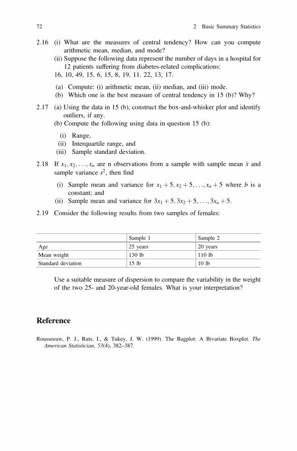
2:16 (i) What are the measures of central tendency? How can you computearithmetic mean, median, and mode?
(ii) Suppose the following data represent the number of days in a hospital for12 patients suffering from diabetes-related complications:
16, 10, 49, 15, 6, 15, 8, 19, 11. 22, 13, 17.
(a) Compute: (i) arithmetic mean, (ii) median, and (iii) mode.(b) Which one is the best measure of central tendency in 15 (b)? Why?
2:17 (a) Using the data in 15 (b), construct the box-and-whisker plot and identifyoutliers, if any.
(b) Compute the following using data in question 15 (b):
(i) Range,(ii) Interquartile range, and(iii) Sample standard deviation.
2:18 If x1; x2; . . .; xn are n observations from a sample with sample mean �x andsample variance s2, then find
(i) Sample mean and variance for x1 þ 5; x2 þ 5; . . .; xn þ 5 where b is aconstant; and
(ii) Sample mean and variance for 3x1 þ 5; 3x2 þ 5; . . .; 3xn þ 5.
2:19 Consider the following results from two samples of females:
Sample 1 Sample 2
Age 25 years 20 years
Mean weight 130 lb 110 lb
Standard deviation 15 lb 10 lb
Use a suitable measure of dispersion to compare the variability in the weightof the two 25- and 20-year-old females. What is your interpretation?
Reference
Rousseeuw, P. J., Ruts, I., & Tukey, J. W. (1999). The Bagplot: A Bivariate Boxplot. TheAmerican Statistician, 53(4), 382–387.
72 2 Basic Summary Statistics

Chapter 3Basic Probability Concepts
3.1 General Definitions and Concepts
As we have defined statistics, in broad terms, it deals with two major components,descriptive measures, and inference. Probability is the foundation for makinginference about the population based on the sample as representative part of thepopulation. In other words, probability is the link between population and sample insuch a way that we can have an understanding about the degree of uncertainty inmaking decision about the population characteristics on the basis of sample char-acteristics with the help of underlying probabilities.
ProbabilityProbability is a measure used to measure the chance of the occurrence of someevent. Probability measure ranges from 0 to 1, where 0 indicates impossibility and 1indicates the certainty of the occurrence of an event.
ExperimentAn experiment is a procedure (or process) that we perform whose outcomes are notpredictable in advance.
Example: Experiment with coin tossing results in two outcomes, head or tail, butthe outcome is not known until the coin is tossed or until the experiment is con-ducted. Here, the two outcomes, head and tail, are exhaustive, because one of thesetwo outcomes must occur in each experiment and there are no other possibleoutcomes in this experiment.
Sample SpaceThe sample space of an experiment is the set of all possible outcomes of anexperiment. Also, it is called the universal set and is denoted by X.
Example In the coin tossing experiment with a single coin, the possible outcomesare head (H) or tail (T). Hence, the sample space is X ¼ H; Tf g.
© Springer Nature Singapore Pte Ltd. 2018M. A. Islam and A. Al-Shiha, Foundations of Biostatistics,https://doi.org/10.1007/978-981-10-8627-4_3
73
EventAny subset of the sample space X is called an event. For example, in the cointossing experiment, an event called success may occur if the outcome is a head (H).If a tail (T) appears, then it may be called failure. It may be noted that
(i) / � X is an event is an impossible event, and(ii) X � X is an event is a sure or certain event.
An example is shown here to illustrate the sample space and events.Let us consider selecting a patient from a hospital room with six beds numbered
from 1 to 6 and observing the patient of the selected bed. Here, the patients areidentified by their respective bed numbers.
This experiment has six possible outcomes or elements.The sample space is X ¼ 1; 2; 3; 4; 5; 6f g.Consider the following events and the elements corresponding to the events:
E1 = getting an even number ¼ 2; 4; 6f g � X,E2 = getting a number less than 4 ¼ 1; 2; 3f g � X,E3 = getting 1 or 3 ¼ 1; 3f g � X,E4 = getting an odd number ¼ 1; 3; 5f g � X,E5 = getting a negative number ¼ fg ¼ / � X, andE6 = getting a number less than 10 ¼ 1; 2; 3; 4; 5; 6f g ¼ X � X.
Notation nðXÞ = number of outcomes (elements) in X andnðEÞ = number of outcomes (elements) in the event E.
Equally Likely OutcomesThe outcomes of an experiment are equally likely if the outcomes have the samechance of occurrence. In other words, an experiment resulting in equally likelyoutcomes is equally probable. It implies that if the sample space contains n equallylikely outcomes, then it is likely that probability of each outcome is 1/n. In case ofthe coin tossing example, the outcomes are (H, T) and the outcomes are equallylikely for a fair coin. The probabilities of outcomes, Head or Tail, are equally likelywith probability 1/2 for each outcome.
Mutually Exclusive OutcomesIn an experiment, if only one outcome is observed at a time excluding the occur-rence of any other outcome, then it is called mutually exclusive.
Example: In the coin tossing experiment, if the outcome is observed to be head,the occurrence of tail is not possible at the same time and vice versa.
3.2 Probability of an Event
If the experiment has nðXÞ equally likely outcomes, then the probability of theevent E is denoted by P(E) and is defined by:
74 3 Basic Probability Concepts

PðEÞ ¼ nðEÞnðXÞ ¼
number of outcomes in Enumber of outcomes in X
:
This is the classical definition of probability and under this definition the ex-periment should satisfy the condition of equally likely as an essential preconditionwhich may not be true in many practical situations.Example: If we conduct an experiment with a fair coin, then the outcomes H orT are equally likely but if we consider outcomes of defective and non-defectiveproducts from an experiment, the condition of equally likely outcomes may beviolated because outcomes are not necessarily equally likely. In that case, we mayuse an alternative definition known as the relative frequency or empirical definitionto measure the probability as stated below.
Let an event E occurs nðEÞ times in a series of n trials, where n is the totalnumber of trials or sample size, the trials are conducted under the same conditions
in the experiment. Here, the ratio nðEÞn is the relative frequency of the event E in
n trials. If n tends to infinity, then we can define the probability of E as follows:
PðEÞ ¼ limn!1
nðEÞn
:
Example 3.1 (Example of Classical Probability)In the experiment for selecting patients identified by bed number of six patients
as discussed in the previous example, suppose the bed number is selected at ran-dom. Determine the probabilities of the following events:
E1 = the patient staying in a bed with even number,E2 = the patient staying in a bed with a number less than 4, andE3 = the patient staying in a bed with numbers 1 or 3.
Solution
X ¼ 1; 2; 3; 4; 5; 6f g ; n Xð Þ ¼ 6E1 ¼ 2; 4; 6f g ; n E1ð Þ ¼ 3E2 ¼ 1; 2; 3f g ; n E2ð Þ ¼ 3E3 ¼ 1; 3f g ; n E3ð Þ ¼ 2
The outcomes are equally likely. Then, by definition the probabilities of theevents, E1;E2; andE3 are
P E1ð Þ ¼ 36; P E2ð Þ ¼ 3
6; and P E3ð Þ ¼ 2
6:
Some Operations on EventsLet A and B be two events defined on the sample space X.
3.2 Probability of an Event 75

(i) Union of Two events: (A[B)The event A[B consists of all outcomes in A or in B or in both A and B. Theevent A[B occurs if A occurs, or B occurs, or both A and B occur.
(ii) Intersection of Two Events: (A\B)The event A\B consists of all outcomes in both A and B. The event A\Boccurs if both A and B occur.
(iii) Complement of an Event: (A) or (AC) or (A0)The complement of the event A is denoted by A. The event A consists of alloutcomes of X that are not in A. The event A occurs if A does not.
Example 3.2 (Classical Probability)Experiment: Selecting a patient randomly from a hospital room having six beds
numbered 1, 2, 3, 4, 5, and 6.Define the following events:
E1 ¼ 2; 4; 6f g = selected an even number.E2 ¼ 1; 2; 3f g = selecting a number <4.E4 ¼ 1; 3; 5f g = selecting an odd number.
76 3 Basic Probability Concepts

(1) E1 [E2 ¼ 1; 2; 3; 4; 6f g ¼ selecting an even number or a number less than 4:
P E1 [E2ð Þ ¼ n E1 [E2ð Þn Xð Þ ¼ 5
6
(2) E1 [E4 ¼ 1; 2; 3; 4; 5; 6f g ¼ X ¼ selecting an even number or an odd number:
P E1 [E4ð Þ ¼ n E1 [E4ð Þn Xð Þ ¼ 6
6¼ 1:
It can be shown that E1 [E4 ¼ X where E1 and E4 are called exhaustive events.The union of these events gives the whole sample space.
(3) E1 \E2 ¼ 2f g = selecting an even number and a number less than 4.
P E1 \E2ð Þ ¼ n E1 \E2ð Þn Xð Þ ¼ 1
6
3.2 Probability of an Event 77
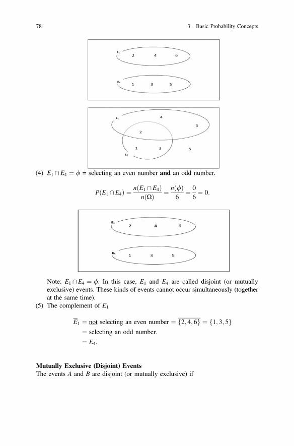
(4) E1 \E4 ¼ / = selecting an even number and an odd number.
P E1 \E4ð Þ ¼ n E1 \E4ð Þn Xð Þ ¼ n /ð Þ
6¼ 0
6¼ 0:
Note: E1 \E4 ¼ /. In this case, E1 and E4 are called disjoint (or mutuallyexclusive) events. These kinds of events cannot occur simultaneously (togetherat the same time).
(5) The complement of E1
E1 ¼ not selecting an even number ¼ f2; 4; 6g ¼ 1; 3; 5f g¼ selecting an odd number:
¼ E4:
Mutually Exclusive (Disjoint) EventsThe events A and B are disjoint (or mutually exclusive) if
78 3 Basic Probability Concepts

A\B ¼ /:
In this case, it is impossible that both events occur simultaneously (i.e., togetherin the same time). Hence,
(i) P A\Bð Þ ¼ 0(ii) P A[Bð Þ ¼ PðAÞþPðBÞ:
If A \ B 6¼ /, then A and B are not mutually exclusive (not disjoint).
A \ B 6¼ / A \ B = /
A and B are not mutually exclusive A and B are mutually exclusive (disjoint)
It is possible that both events may occur at thesame time.
It is impossible that both events occur at thesame time.
Exhaustive EventsThe events A1;A2; . . .;An are exhaustive events if
A1 [A2 [ . . .[An ¼ X:
For this case, P A1 [A2 [ . . .[Anð Þ ¼ PðXÞ ¼ 1.
Note
1. A[A ¼ X (A and A are exhaustive events),2. A\A ¼ / (A and A are mutually exclusive (disjoint) events),3. nðAÞ ¼ nðXÞ � nðAÞ, and4. P A
� � ¼ 1� PðAÞ.
3.2 Probability of an Event 79
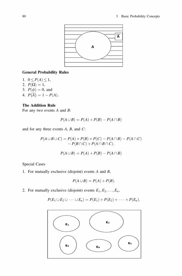
General Probability Rules
1. 0�P Að Þ� 1,2. P Xð Þ ¼ 1,3. P /ð Þ ¼ 0, and4. P A
� � ¼ 1� P Að Þ.
The Addition RuleFor any two events A and B:
P A[Bð Þ ¼ P Að ÞþP Bð Þ � P A\Bð Þ
and for any three events A, B, and C:
PðA[B[CÞ ¼ PðAÞþPðBÞþPðCÞ � PðA\BÞ � PðA\CÞ� PðB\CÞþPðA\B\CÞ:
P A[Bð Þ ¼ P Að ÞþP Bð Þ � P A\Bð Þ
Special Cases
1. For mutually exclusive (disjoint) events A and B,
P A[Bð Þ ¼ P Að ÞþP Bð Þ:
2. For mutually exclusive (disjoint) events E1;E2; . . .;En,
P E1 [E2 [ � � � [Enð Þ ¼ P E1ð ÞþP E2ð Þþ � � � þP Enð Þ:
80 3 Basic Probability Concepts
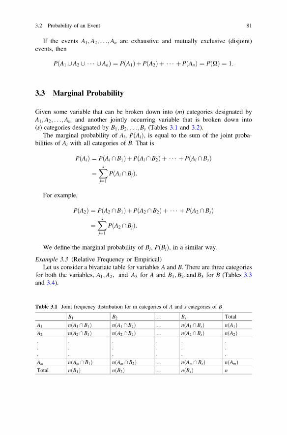
If the events A1;A2; . . .;An are exhaustive and mutually exclusive (disjoint)events, then
P A1 [A2 [ � � � [Anð Þ ¼ P A1ð ÞþP A2ð Þþ � � � þP Anð Þ ¼ PðXÞ ¼ 1:
3.3 Marginal Probability
Given some variable that can be broken down into (m) categories designated byA1;A2; . . .;Am and another jointly occurring variable that is broken down into(s) categories designated by B1;B2; . . .;Bs (Tables 3.1 and 3.2).
The marginal probability of Ai, PðAiÞ, is equal to the sum of the joint proba-bilities of Ai with all categories of B. That is
PðAiÞ ¼ PðAi \B1ÞþPðAi \B2Þþ � � � þPðAi \BsÞ
¼Xs
j¼1
PðAi \BjÞ:
For example,
PðA2Þ ¼ PðA2 \B1ÞþPðA2 \B2Þþ � � � þPðA2 \BsÞ
¼Xs
j¼1
PðA2 \BjÞ:
We define the marginal probability of Bj, PðBjÞ, in a similar way.
Example 3.3 (Relative Frequency or Empirical)Let us consider a bivariate table for variables A and B. There are three categories
for both the variables, A1;A2; and A3 for A and B1;B2; andB3 for B (Tables 3.3and 3.4).
Table 3.1 Joint frequency distribution for m categories of A and s categories of B
B1 B2 … Bs Total
A1 nðA1 \B1Þ nðA1 \B2Þ … nðA1 \BsÞ nðA1ÞA2 nðA2 \B1Þ nðA2 \B2Þ … nðA2 \BsÞ nðA2Þ...
.
.
.
.
.
.
.
.
.
.
.
.
.
.
.
Am nðAm \B1Þ nðAm \B2Þ … nðAm \BsÞ nðAmÞTotal nðB1Þ nðB2Þ … nðBsÞ n
3.2 Probability of an Event 81
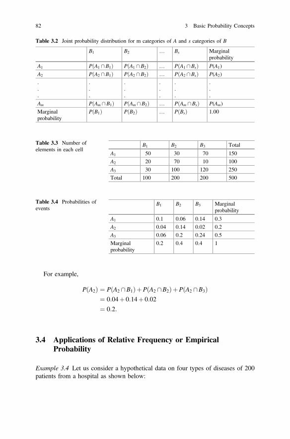
For example,
PðA2Þ ¼ PðA2 \B1ÞþPðA2 \B2ÞþPðA2 \B3Þ¼ 0:04þ 0:14þ 0:02
¼ 0:2:
3.4 Applications of Relative Frequency or EmpiricalProbability
Example 3.4 Let us consider a hypothetical data on four types of diseases of 200patients from a hospital as shown below:
Table 3.2 Joint probability distribution for m categories of A and s categories of B
B1 B2 … Bs Marginalprobability
A1 PðA1 \B1Þ PðA1 \B2Þ … PðA1 \BsÞ P(A1)
A2 PðA2 \B1Þ PðA2 \B2Þ … PðA2 \BsÞ P(A2)
.
.
.
.
.
.
.
.
.
.
.
.
.
.
.
.
.
.
Am PðAm \B1Þ PðAm \B2Þ … PðAm \BsÞ P(Am)
Marginalprobability
PðB1Þ PðB2Þ … PðBsÞ 1.00
Table 3.3 Number ofelements in each cell
B1 B2 B3 Total
A1 50 30 70 150
A2 20 70 10 100
A3 30 100 120 250
Total 100 200 200 500
Table 3.4 Probabilities ofevents
B1 B2 B3 Marginalprobability
A1 0.1 0.06 0.14 0.3
A2 0.04 0.14 0.02 0.2
A3 0.06 0.2 0.24 0.5
Marginalprobability
0.2 0.4 0.4 1
82 3 Basic Probability Concepts

Disease type A B C D Total
Number of patients 90 80 20 10 200
Experiment: Selecting a patient at random and observe his/her disease type.Total number of trials, sample size, in this case, is
n ¼ 200:Define the events
E1 = the disease type of the selected patient is A,E2 = the disease type of the selected patient is B,E3 = the disease type of the selected patient is C, andE4 = the disease type of the selected patient is D.
Number of elements for each event is shown below:
n E1ð Þ ¼ 90; n E2ð Þ ¼ 80;n E3ð Þ ¼ 20; n E4ð Þ ¼ 10:
Probabilities of the events are
P E1ð Þ ¼ 90200
¼ 0:45; P E2ð Þ ¼ 80200
� 0:40;
P E3ð Þ ¼ 20200
¼ 0:1; P E4ð Þ ¼ 10200
¼ 0:05:
Some Operations on the Events
1. E2 \E4 = the disease type of the selected patients is “B” and “D”.E2 \E4 ¼ / (disjoint events/mutually exclusive events)
PðE2 \E4Þ ¼ Pð/Þ ¼ 0:
2. E2 [E4 = the disease type of the selected patients is “B” or “D”.
PðE2 [E4Þ ¼n E2 [E4ð Þ
n Xð Þ ¼ 80þ 10200
¼ 90200
¼ 0:45
or
P E2ð ÞþP E4ð Þ ¼ 80200
þ 10200
¼ 90200
¼ 0:45;
8>><>>:
since E2 \E4 ¼ /.3. E1 = the disease type of the selected patients is not “A”.
nðE1Þ ¼ n� nðE1Þ ¼ 200� 90 ¼ 110
PðE1Þ ¼ nðE1Þn
¼ 110200
¼ 0:55:
3.4 Applications of Relative Frequency or Empirical Probability 83
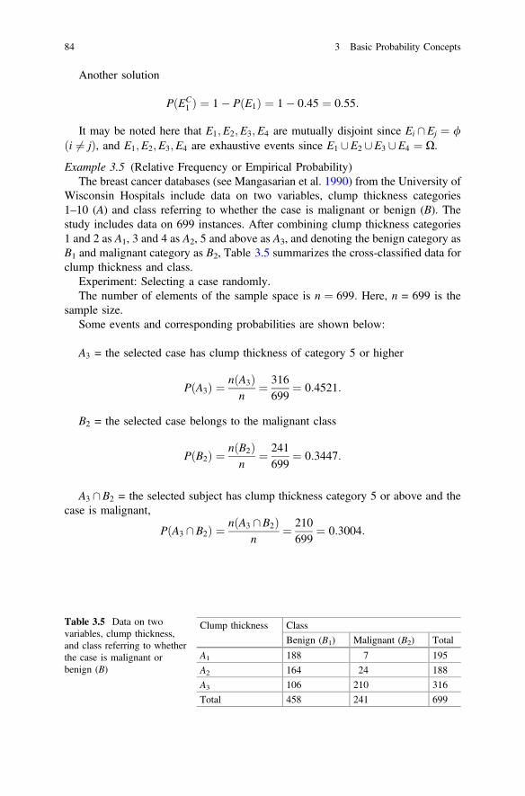
Another solution
PðEC1 Þ ¼ 1� PðE1Þ ¼ 1� 0:45 ¼ 0:55:
It may be noted here that E1;E2;E3;E4 are mutually disjoint since Ei \Ej ¼ /i 6¼ jð Þ, and E1;E2;E3;E4 are exhaustive events since E1 [E2 [E3 [E4 ¼ X.
Example 3.5 (Relative Frequency or Empirical Probability)The breast cancer databases (see Mangasarian et al. 1990) from the University of
Wisconsin Hospitals include data on two variables, clump thickness categories1–10 (A) and class referring to whether the case is malignant or benign (B). Thestudy includes data on 699 instances. After combining clump thickness categories1 and 2 as A1, 3 and 4 as A2, 5 and above as A3, and denoting the benign category asB1 and malignant category as B2, Table 3.5 summarizes the cross-classified data forclump thickness and class.
Experiment: Selecting a case randomly.The number of elements of the sample space is n ¼ 699. Here, n = 699 is the
sample size.Some events and corresponding probabilities are shown below:
A3 = the selected case has clump thickness of category 5 or higher
P A3ð Þ ¼ n A3ð Þn
¼ 316699
¼ 0:4521:
B2 = the selected case belongs to the malignant class
P B2ð Þ ¼ n B2ð Þn
¼ 241699
¼ 0:3447:
A3 \B2 = the selected subject has clump thickness category 5 or above and thecase is malignant,
P A3 \B2ð Þ ¼ n A3 \B2ð Þn
¼ 210699
¼ 0:3004:
Table 3.5 Data on twovariables, clump thickness,and class referring to whetherthe case is malignant orbenign (B)
Clump thickness Class
Benign (B1) Malignant (B2) Total
A1 188 7 195
A2 164 24 188
A3 106 210 316
Total 458 241 699
84 3 Basic Probability Concepts
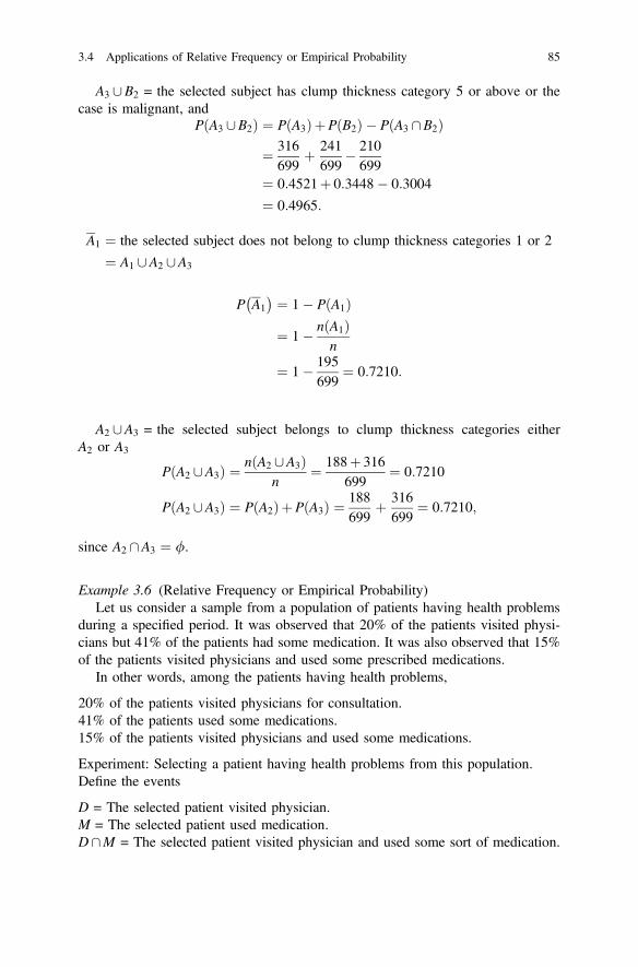
A3 [B2 = the selected subject has clump thickness category 5 or above or thecase is malignant, and
P A3 [B2ð Þ ¼ P A3ð ÞþP B2ð Þ � P A3 \B2ð Þ¼ 316
699þ 241
699� 210699
¼ 0:4521þ 0:3448� 0:3004
¼ 0:4965:
A1 ¼ the selected subject does not belong to clump thickness categories 1 or 2
¼ A1 [A2 [A3
P A1� � ¼ 1� P A1ð Þ
¼ 1� n A1ð Þn
¼ 1� 195699
¼ 0:7210:
A2 [A3 = the selected subject belongs to clump thickness categories eitherA2 or A3
P A2 [A3ð Þ ¼ n A2 [A3ð Þn
¼ 188þ 316699
¼ 0:7210
P A2 [A3ð Þ ¼ P A2ð ÞþP A3ð Þ ¼ 188699
þ 316699
¼ 0:7210;
since A2 \A3 ¼ /.
Example 3.6 (Relative Frequency or Empirical Probability)Let us consider a sample from a population of patients having health problems
during a specified period. It was observed that 20% of the patients visited physi-cians but 41% of the patients had some medication. It was also observed that 15%of the patients visited physicians and used some prescribed medications.
In other words, among the patients having health problems,
20% of the patients visited physicians for consultation.41% of the patients used some medications.15% of the patients visited physicians and used some medications.
Experiment: Selecting a patient having health problems from this population.Define the events
D = The selected patient visited physician.M = The selected patient used medication.D\M = The selected patient visited physician and used some sort of medication.
3.4 Applications of Relative Frequency or Empirical Probability 85
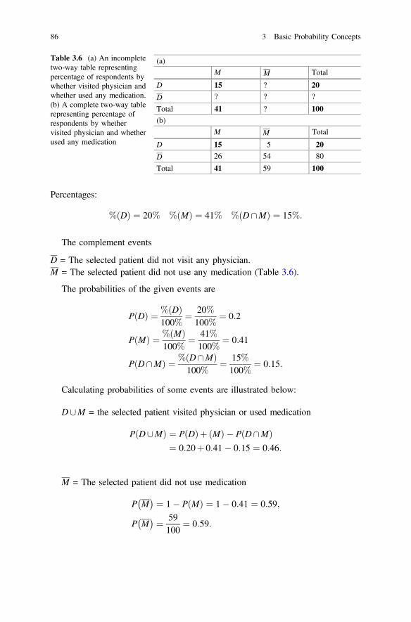
Percentages:
% Dð Þ ¼ 20% % Mð Þ ¼ 41% % D\Mð Þ ¼ 15%:
The complement events
D = The selected patient did not visit any physician.M = The selected patient did not use any medication (Table 3.6).
The probabilities of the given events are
P Dð Þ ¼ % Dð Þ100%
¼ 20%100%
¼ 0:2
P Mð Þ ¼ % Mð Þ100%
¼ 41%100%
¼ 0:41
P D\Mð Þ ¼ % D\Mð Þ100%
¼ 15%100%
¼ 0:15:
Calculating probabilities of some events are illustrated below:
D[M = the selected patient visited physician or used medication
P D[Mð Þ ¼ P Dð Þþ Mð Þ � P D\Mð Þ¼ 0:20þ 0:41� 0:15 ¼ 0:46:
M = The selected patient did not use medication
P M� � ¼ 1� P Mð Þ ¼ 1� 0:41 ¼ 0:59;
P M� � ¼ 59
100¼ 0:59:
Table 3.6 (a) An incompletetwo-way table representingpercentage of respondents bywhether visited physician andwhether used any medication.(b) A complete two-way tablerepresenting percentage ofrespondents by whethervisited physician and whetherused any medication
(a)
M M Total
D 15 ? 20
D ? ? ?
Total 41 ? 100(b)
M M Total
D 15 5 20
D 26 54 80
Total 41 59 100
86 3 Basic Probability Concepts

D = The selected patient did not visit physician
P D� � ¼ 1� P Dð Þ ¼ 1� 0:20 ¼ 0:80;
P D� � ¼ 80
100¼ 0:80:
D\M = the selected patient did not visit physician and did not use medication.
P D\M� � ¼ 54
100¼ 0:54:
D\M = the selected patient did not visit physician and used medication.
P D\M� � ¼ 5
100¼ 0:05:
D\M = the selected patient visited physician and did not use medication.
P D\M� � ¼ 5
100¼ 0:05:
D[M = the selected patient visited physician or did not use medication.
P D[M� � ¼ P Dð Þþ M
� �� P D\M� �
¼ 0:20þ 0:59� 0:26 ¼ 0:53:
D[M = the selected patient did not visit physician or used medication.
P D[M� � ¼ P D
� �þ Mð Þ � P D\M� �
¼ 0:80þ 0:41� 0:26 ¼ 0:95:
D[M = the selected patient did not visit physician or did not use medication.
P D[M� � ¼ P D
� �þ M� �� P D\M
� �¼ 0:80þ 0:59� 0:54 ¼ 0:85:
3.5 Conditional Probability
The conditional probability of the event A when we know that the event B hasalready occurred is defined by
3.4 Applications of Relative Frequency or Empirical Probability 87

P AjBð Þ ¼ P A\Bð ÞP Bð Þ ; P Bð Þ 6¼ 0:
P(A|B) = The conditional probability of A given B.The following figure shows the events graphically:
Notes:
1. P AjBð Þ ¼ P A\Bð ÞP Bð Þ ¼ n A\Bð Þ=n Xð Þ
n Bð Þ=n Xð Þ ¼ n A\Bð Þn Bð Þ
2. P BjAð Þ ¼ P A\Bð ÞP Að Þ
3. For calculating P AjBð Þ, we may use any one of the following:
i. P AjBð Þ ¼ P A\Bð ÞP Bð Þ
ii. P AjBð Þ ¼ n A\Bð Þn Bð Þ
iii. Using the restricted table directly.
Multiplication Rules of ProbabilityFor any two events A and B, we have
P A\Bð Þ ¼ P Bð ÞP AjBð Þ;P A\Bð Þ ¼ P Að ÞP BjAð Þ:
Example 3.7 Let us consider a hypothetical set of data on 600 adult males classifiedby their ages and smoking habits as summarized in Table 3.7.
Consider the following event:(B1|A2) = smokes daily given that age is between 30 and 39
Table 3.7 Two-way table displaying number of respondents by age and smoking habit ofrespondents smoking habit
Daily B1ð Þ Occasionally B2ð Þ Not at all B3ð Þ Total
Age 20–29 A1ð Þ 57 18 13 88
30–39 A2ð Þ 200 55 90 345
40–49 A3ð Þ 50 40 55 145
50+ A4ð Þ 7 0 15 22
Total 314 113 173 600
88 3 Basic Probability Concepts

P B1ð Þ ¼ nðB1Þn
¼ 314600
¼ 0:523
P B1jA2ð Þ ¼ P B1 \A2ð ÞP A2ð Þ
¼ 0:3330:575
¼ 0:579
P B1 \A2ð Þ ¼ n B1 \A2ð Þn ¼ 200
600 ¼ 0:333
P A2ð Þ ¼ n A2ð Þn ¼ 345
600 ¼ 0:575
( )
Another solution
P B1jA2ð Þ ¼ n B1 \A2ð Þn A2ð Þ ¼ 200
345¼ 0:579:
Notice that
P B1ð Þ ¼ 0:523
P B1jA2ð Þ ¼ 0:579
P B1jA2ð Þ[P B1ð Þ; P B1ð Þ 6¼ P B1jA2ð Þ:
Example 3.8 (Multiplication Rule of Probability)It was found from a study that 20% of the patients with some general health
problems visited physicians and out of those who visited physicians 75% wereprescribed some medications. If a person with health problem is selected randomlyfrom the population, what is the probability that the person will use medicine? Whatis the percentage of patients who use medication?
SolutionDefine the following events:
A = the event of visiting physician,B = the event of using medication, andA\B ¼ the event of visiting physician and using medication
¼ the event of experiencing both events:
Therefore, the probability of visiting physician and using medication is P(A\B).From the given information, the probability of visiting physician is
P Að Þ ¼ 0:220%100%
¼ 0:2� �
:
3.5 Conditional Probability 89
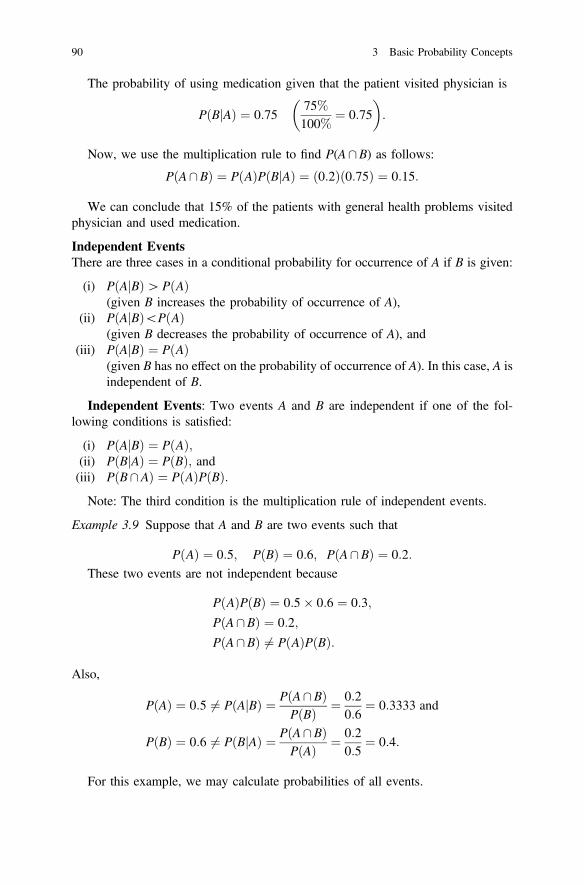
The probability of using medication given that the patient visited physician is
P BjAð Þ ¼ 0:7575%100%
¼ 0:75� �
:
Now, we use the multiplication rule to find P(A\B) as follows:
PðA\BÞ ¼ P Að ÞP BjAð Þ ¼ 0:2ð Þ 0:75ð Þ ¼ 0:15:
We can conclude that 15% of the patients with general health problems visitedphysician and used medication.
Independent EventsThere are three cases in a conditional probability for occurrence of A if B is given:
(i) P AjBð Þ[P Að Þ(given B increases the probability of occurrence of A),
(ii) P AjBð Þ\P Að Þ(given B decreases the probability of occurrence of A), and
(iii) P AjBð Þ ¼ P Að Þ(given B has no effect on the probability of occurrence of A). In this case, A isindependent of B.
Independent Events: Two events A and B are independent if one of the fol-lowing conditions is satisfied:
(i) P AjBð Þ ¼ P Að Þ;(ii) P BjAð Þ ¼ P Bð Þ; and(iii) P B\Að Þ ¼ P Að ÞP Bð Þ:Note: The third condition is the multiplication rule of independent events.
Example 3.9 Suppose that A and B are two events such that
P Að Þ ¼ 0:5; P Bð Þ ¼ 0:6; PðA\BÞ ¼ 0:2:These two events are not independent because
P Að ÞP Bð Þ ¼ 0:5� 0:6 ¼ 0:3;
PðA\BÞ ¼ 0:2;
PðA\BÞ 6¼ P Að ÞP Bð Þ:
Also,
PðAÞ ¼ 0:5 6¼ PðAjBÞ ¼ PðA\BÞPðBÞ ¼ 0:2
0:6¼ 0:3333 and
PðBÞ ¼ 0:6 6¼ PðBjAÞ ¼ PðA\BÞPðAÞ ¼ 0:2
0:5¼ 0:4:
For this example, we may calculate probabilities of all events.
90 3 Basic Probability Concepts

We can use a two-way table of the probabilities as follows:
B B Total
A 0.2 ? 0.5
A ? ? ?
Total 0.6 ? 1.00
We complete Table 3.8:
PðAÞ ¼ 0:5
PðBÞ ¼ 0:4
PðA\BÞ ¼ 0:3
PðA\BÞ ¼ 0:4
PðA\BÞ ¼ 0:1
PðA[BÞ ¼ PðAÞþPðBÞ � PðA\BÞ ¼ 0:5þ 0:6� 0:2 ¼ 0:9
PðA[BÞ ¼ PðAÞþPðBÞ � PðA\BÞ ¼ 0:5þ 0:4� 0:3 ¼ 0:6:
The Addition Rule for Independent EventsIf the events A and B are independent, then
P A[Bð Þ ¼ P Að ÞþP Bð Þ � P A\Bð Þ¼ P Að ÞþP Bð Þ � PðAÞPðBÞ:
Example 3.10 Suppose that 12 patients admitted with fever (F = high fever,F = low fever) in a hospital are selected randomly and asked their opinion aboutwhether they were satisfied with the services in the hospital (S = satisfied, S = notsatisfied). The table below summarizes the data.
F (high fever) F (low fever) Total
S (satisfied) 2 1 3
S (not satisfied) 6 3 9
Total 8 4 12
The experiment is to randomly choose one of these patients. Consider the fol-lowing events:
Table 3.8 A two-way tabledisplaying probabilities
B B Total
A 0.2 0.3 0.5
A 0.4 0.1 0.5
Total 0.6 0.4 1.00
3.5 Conditional Probability 91

S = satisfied with service andF = high fever.
(a) Find the probabilities of the following events:
1. the chosen patient is satisfied with service in the hospital,2. the chosen patient is suffering from high fever,3. the chosen patient is satisfied with service and suffering from high fever, and4. the chosen patient is satisfied with service and is not suffering from high
fever.
(b) Find the probability of choosing a patient who is suffering from high fevergiven that the patient has high fever.
(c) Are the events S and F independent? Why?(d) Are the events S and F disjoint? Why?
Solution
(a) The experiment has n = 12.P(patient is satisfied with service)
P Sð Þ ¼ nðSÞn
¼ 312
¼ 0:25:
P(patient suffers from high fever)
P Fð Þ ¼ nðFÞn
¼ 812
¼ 0:6667:
P(satisfied with service and suffers from high fever)
PðS\FÞ ¼ nðS\FÞn
¼ 212
¼ 0:16667:
P(satisfied with service and does not suffer from high fever)
PðS\FÞ ¼ nðS\FÞn
¼ 112
¼ 0:0833:
(b) The probability of selecting a patient who suffers from high fever given that thepatient is satisfied with service is
PðFjSÞ ¼ PðS\FÞPðSÞ ¼ 2=12
0:25¼ 0:6667:
(c) The events S and F are independent because PðFjSÞ ¼ PðFÞ.(d) The events S and F are not disjoint because S\F 6¼ /; nðS\FÞ ¼ 2.
92 3 Basic Probability Concepts

3.6 Conditional Probability, Bayes’ Theorem,and Applications
Bayes’ theorem gives a posterior probability using the estimate used for a priorprobability. This procedure is performed using the concept of the conditionalprobability. Let us consider that there are two states regarding the disease and twostates stating the result of a test then the outcomes are
We define the following events:
D: the individual has the disease (presence of the disease),D: the individual does not have the disease (absence of the disease),T: the individual has a positive screening test result, andT : the individual has a negative screening test result.
There are four possible situations as shown in the following table:
Status of the disease
+ve (D: Present) −ve (D: Absent)
Result of the test +ve (T) Correct diagnosis False positive result
−ve (T) False-negative result Correct diagnosis
We are interested in the true status of the disease for given test result which is aposterior probability. This is essentially a conditional probability, for instance,probability of being suffered from disease for the given fact that the screening testresult shows positive. On the other hand, the estimate of the prevalence of thedisease in the population may be considered as the prior probability which is amarginal probability and does not depend on any other condition. This helps us tounderstand or confirm how good the true status of the disease is for a given testresult.
There are two false results that can happen in an experiment concerning diseasestatus and test results.
1. A false-positive result: This is defined by a conditional probability
PðT jDÞ ¼ P positive resultjabsence of the diseaseð Þ
and this result happens when a test shows a positive status if the true status isknown to be negative.
3.6 Conditional Probability, Bayes’ Theorem, and Applications 93

2. A false-negative result: The false negative can be defined by the followingconditional probability:
PðT jDÞ ¼ P negative resultjpresence of the diseaseð Þ;
where the conditional probability states that a test shows a negative status;however, the true status is known to be positive.
Two Important Measures: The Sensitivity and Specificity of a Test
1. The Sensitivity: The conditional probability of a positive test given that thedisease status is the presence of disease is
PðT jDÞ ¼ P positive result of the testjpresence of the diseaseð Þ;
which is known as sensitivity of a test.2. The specificity: The specificity is defined as
PðT jDÞ ¼ P negative result of the testjabsence of the diseaseð Þ;
which is the probability of a negative test result given the absence of the disease.
To clarify these concepts, suppose we have a sample of (n) subjects who arecross-classified according to disease status and screening test result (Table 3.9).
For example, there are “a” subjects who have the disease and whose screeningtest result was positive.
From this table, we may compute the following conditional probabilities:
1. The probability of false-positive result
PðTjDÞ ¼ nðT \DÞnðDÞ ¼ b
bþ d:
2. The probability of false negative result
PðTjDÞ ¼ nðT \DÞnðDÞ ¼ c
aþ c:
Table 3.9 Table displayingtest result and true status ofdisease
Test result Disease
Present (D) Absent (D) Total
Positive (T) a b a + b = n(T)
Negative(T)
c d c + d = n(T)
Total a + c = n(D)
b + d = n(D)
n
94 3 Basic Probability Concepts
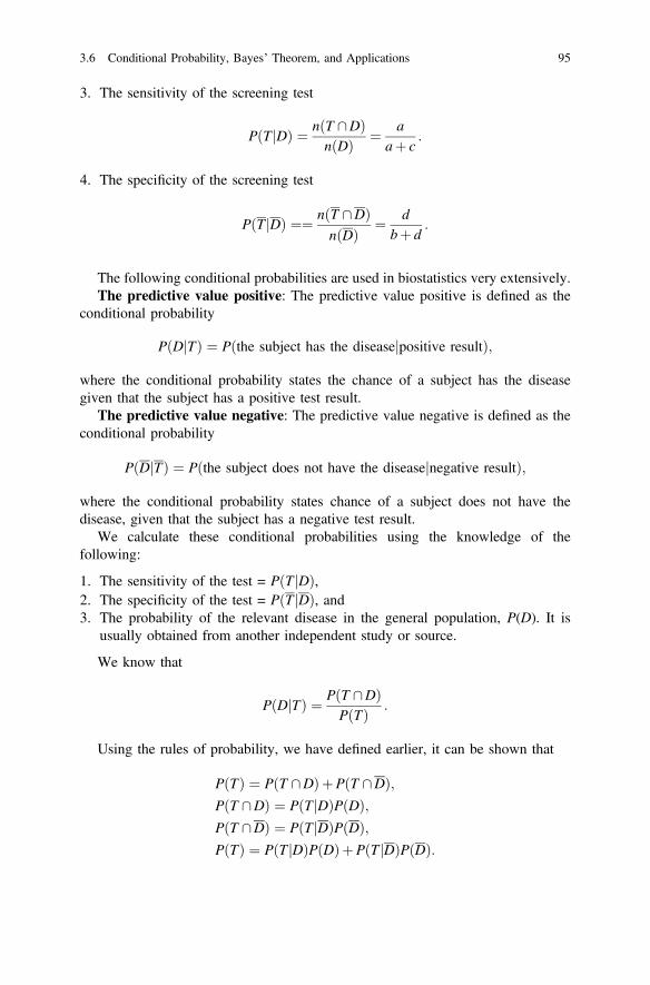
3. The sensitivity of the screening test
PðTjDÞ ¼ nðT \DÞnðDÞ ¼ a
aþ c:
4. The specificity of the screening test
PðTjDÞ ¼¼ nðT \DÞnðDÞ ¼ d
bþ d:
The following conditional probabilities are used in biostatistics very extensively.The predictive value positive: The predictive value positive is defined as the
conditional probability
PðDjTÞ ¼ P the subject has the diseasejpositive resultð Þ;
where the conditional probability states the chance of a subject has the diseasegiven that the subject has a positive test result.
The predictive value negative: The predictive value negative is defined as theconditional probability
PðDjTÞ ¼ P the subject does not have the diseasejnegative resultð Þ;
where the conditional probability states chance of a subject does not have thedisease, given that the subject has a negative test result.
We calculate these conditional probabilities using the knowledge of thefollowing:
1. The sensitivity of the test = PðTjDÞ,2. The specificity of the test = PðTjDÞ, and3. The probability of the relevant disease in the general population, P(D). It is
usually obtained from another independent study or source.
We know that
PðDjTÞ ¼ PðT \DÞPðTÞ :
Using the rules of probability, we have defined earlier, it can be shown that
PðTÞ ¼ PðT \DÞþPðT \DÞ;PðT \DÞ ¼ PðTjDÞPðDÞ;PðT \DÞ ¼ PðTjDÞPðDÞ;PðTÞ ¼ PðT jDÞPðDÞþPðT jDÞPðDÞ:
3.6 Conditional Probability, Bayes’ Theorem, and Applications 95

Therefore, we reach the following version of Bayes’ theorem:
PðDjTÞ ¼ PðT jDÞPðDÞPðTjDÞPðDÞþPðTjDÞPðDÞ :
It is noteworthy that
PðT jDÞ ¼ sensitivity;
PðT jDÞ ¼ 1� PðT jDÞ ¼ 1�specificity;P(D) = The probability of the relevant disease in the general population,
PðDÞ ¼ 1� PðDÞ:
To compute the predictive value negative of a test, we use the followingstatement of Bayes’ theorem:
PðDjTÞ ¼ PðT jDÞPðDÞPðTjDÞPðDÞþPðTjDÞPðDÞ :
It may be noted that PðT jDÞ = specificity and PðT jDÞ ¼ 1� PðTjDÞ =1 − sensitivity.
Example 3.11 Let us consider a study to examine the relationship between diseaseand a screening test result. Two samples were drawn from the population, one forthe patients with symptoms of disease and another sample without symptoms of thedisease. For both the samples, the screening tests were performed in order toconfirm the disease status. The results are summarized in Table 3.10.
Based on another independent study, it is known that the percentage of patientswith disease (the rate of prevalence of the disease) is 8 per 100.
Table 3.10 Table displayingtest result and status ofdisease for the respondentswith or without symptoms ofa disease
Disease status
Test result Present ðDÞ Absent (D) Total
Positive (T) 950 20 970
Negative (T) 50 980 1030
Total 1000 1000 2000
96 3 Basic Probability Concepts

SolutionUsing these data, we estimate the following probabilities:
1. The sensitivity of the test
PðT jDÞ ¼ nðT \DÞnðDÞ ¼ 950
1000¼ 0:95:
2. The specificity of the test:
PðT jDÞ ¼ nðT \DÞnðDÞ ¼ 980
1000¼ 0:98:
3. The probability of the disease in the general population, P(D).
The rate of disease in the relevant general population, P(D), cannot be computedfrom the sample data given in the table. However, it is estimated from a differentstudy that 8% of the population suffered from the disease. Therefore, P(D) can beestimated as
P Dð Þ ¼ 8%100%
¼ 0:08:
4. The predictive value positive of the test.
We wish to estimate the probability that a subject who is positive on the test hasthe disease. We use the Bayes’ theorem as follows:
PðDjTÞ ¼ PðT jDÞPðDÞPðTjDÞPðDÞþPðTjDÞPðDÞ :
From the data displayed in table, we compute
PðT jDÞ ¼ 9501000
¼ 0:95; and
PðT jDÞ ¼ nðT \DÞnðDÞ ¼ 20
1000¼ 0:02:
Substituting these results, we get
PðDjTÞ ¼ ð0:95ÞPðDÞð0:95ÞPðDÞþ ð0:02ÞPðDÞ
¼ 0:95ð Þ 0:08ð Þ0:95ð Þ 0:08ð Þþ 0:02ð Þ 1� 0:08ð Þ ¼ 0:81:
3.6 Conditional Probability, Bayes’ Theorem, and Applications 97

As we see, in this case, the predictive value positive of the test is moderatelyhigh.
5. The predictive value negative of the test
We wish to estimate the probability that a subject who is negative on the testdoes not have the disease. Using the Bayes’ formula, we obtain
PðDjTÞ ¼ PðT jDÞPðDÞPðTjDÞPðDÞþPðTjDÞPðDÞ :
To compute PðDjTÞ, we first compute the following probabilities:
PðT jDÞ ¼ 9801000
¼ 0:98;
PðDÞ ¼ 1� PðDÞ ¼ 1� 0:08 ¼ 0:92;
PðT jDÞ ¼ nðT \DÞnðDÞ ¼ 50
1000¼ 0:05:
Substituting these values, we find
PðDjTÞ ¼ PðTjDÞPðDÞPðT jDÞPðDÞþPðT jDÞPðDÞ
¼ ð0:98Þð0:92Þð0:98Þð0:92Þþ ð0:05Þð0:08Þ
¼ 0:996:
As we see, the predictive value negative is very high.
3.7 Summary
The basic probability concepts are introduced in this chapter. It has been mentionedin Chap. 1 that probability plays a vital role to link the measures based on samplesto the corresponding population values. The concept of random sampling providesthe foundation for such links that depend on the concepts of probability. Thedefinitions of probability along with experiment, sample space, event, equallylikely, and mutually exclusive outcomes are highlighted. The important operationson events are discussed with examples. The concepts of marginal and conditionalprobabilities are discussed in a self-explanatory manner with several examples. Themultiplication rules of probability and the concept of independent events areintroduced in this chapter. The applications of conditional probability and Bayes’theorem in analyzing epidemiological data are shown. The measures of sensitivityand specificity of tests are illustrated with examples.
98 3 Basic Probability Concepts

Exercises
3:1 Three patients are selected at random from a hospital. Consider that at eachdraw it is equally likely that the randomly drawn patient can be either male(M) or female (F).
(i) Write the elements of the sample space.(ii) Write the elements corresponding to the event E = at least one of the
selected patients is female.(iii) Define the event for the subset of sample space containing two male
patients.(iv) Define the subset of sample space containing only male patients.
3:2 In Question 3.1, specify three patients by number of male patients out ofthree randomly selected patients.
(i) Write the elements of the sample space.(ii) Define the subspace of the sample space corresponding to the event
E1 = two or more male patients.(iii) Define the subspace of the space corresponding to the event E2 = less
than two male patients.(iv) Define the subspace of the sample space corresponding to the event
E3 = three male patients.
3:3 Define the subspace of the sample space defined in Question 3.2 for thefollowing events:
(i) E1 [E2;(ii) E1 [E3;(iii) E2 \E3;(iv) E1 [E2 [E3;(v) ðE1 [E2Þ \E3; and(vi) ðE1 \E3Þ [E2:
3:4 Define the subspace of the sample space defined in Question 3.2 for thefollowing events:
(i) E1 [E2;
(ii) E1 [E3;
(iii) E1 \E3;
(iv) E2 \E3;
(v) ðE1 \E2Þ [E3; and(vi) ðE1 \E2Þ \E3:
3:5 For sample space of Exercise 3.2, find the following probabilities:
(i) PðE1Þ;PðE2Þ andPðE3Þ;(ii) PðE1 [E2Þ;
3.7 Summary 99

(iii) PðE1 [E3Þ;(iv) PðE1 \E3Þ;(v) PðE2 \E3Þ;(vi) PðE1 [E2 [E3Þ;(vii) P½ðE1 [E2Þ \E3�; and(viii) P½ðE1 \E3Þ [E2�:
3:6 The following table shows a hypothetical bivariate representation of 100,000pregnant women by maternal age (A) and pregnancy-related deaths (B) in acommunity.
Maternal age in years (A) Pregnancy-related deaths orsurvival (B)
Total
Survived (B1) Died (B2)
<20 (A1) 19,989 11 20,000
20–39 (A2) 59,910 90 60,000
40–49 (A3) 19,993 7 20,000
Total 99,892 108 100,000
Find the following probabilities:
(i) PðA1Þ;PðA2Þ; andPðA3Þ:(ii) PðB1Þ andPðB2Þ:(iii) PðB2jA1Þ;PðB2jA2Þ andPðB2jA3Þ:(iv) PðB1jA1Þ;PðB1jA2Þ andPðB1jA3Þ:(v) Comment on your findings about pregnancy-related deaths and
maternal age for the community.
3:7 In a study on incidence of common flu among the students of a university.Suppose the study was conducted on 200 male and female students during asemester. The data are summarized in the following table:
Gender of students (A) Incidence of flu duringsemester (B)
Total
Yes (Y) No (N)
Male (M) 15 85 100
Female (F) 20 80 100
Total 35 165 200
Suppose we pick a subject randomly from this group. Then, answer thefollowing questions:
(i) Find PðM \ YÞ.(ii) Find PðM \ YÞ.
100 3 Basic Probability Concepts
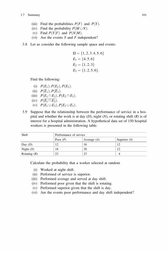
(iii) Find the probabilities PðFÞ and PðYÞ.(iv) Find the probability PðM [NÞ.(v) Find PðY Fj Þ and PðN Mj Þ.(vi) Are the events Y and F independent?
3:8 Let us consider the following sample space and events:
X ¼ 1; 2; 3; 4; 5; 6f gE1 ¼ 4; 5; 6f gE2 ¼ 1; 2; 3f gE3 ¼ 1; 2; 5; 6f g:
Find the following:
(i) PðE1Þ;PðE2Þ;PðE3Þ:(ii) PðE1Þ;PðE3Þ:(iii) PðE1 \E2Þ;PðE2 \E3Þ:(iv) PðE1 \E2Þ:(v) PðE1 [E2Þ;PðE2 [E3Þ:
3:9 Suppose that the relationship between the performance of service in a hos-pital and whether the work is at day (D), night (N), or rotating shift (R) is ofinterest for a hospital administration. A hypothetical data set of 150 hospitalworkers is presented in the following table.
Shift Performance of service
Poor (P) Average (A) Superior (S)
Day (D) 12 16 12
Night (N) 18 30 12
Rotating (R) 23 23 4
Calculate the probability that a worker selected at random
(i) Worked at night shift.(ii) Performed of service is superior.(iii) Performed average and served at day shift.(iv) Performed poor given that the shift is rotating.(v) Performed superior given that the shift is day.(vi) Are the events poor performance and day shift independent?
3.7 Summary 101
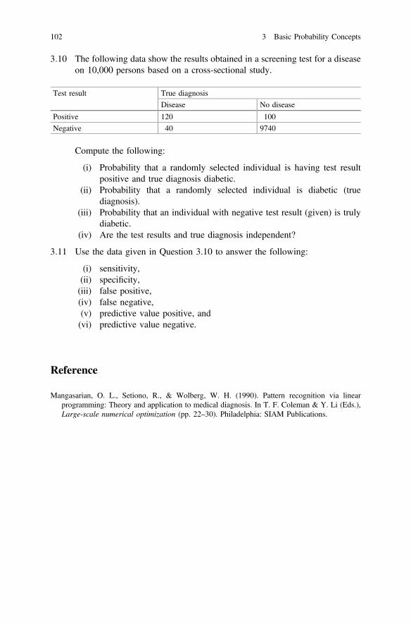
3:10 The following data show the results obtained in a screening test for a diseaseon 10,000 persons based on a cross-sectional study.
Test result True diagnosis
Disease No disease
Positive 120 100
Negative 40 9740
Compute the following:
(i) Probability that a randomly selected individual is having test resultpositive and true diagnosis diabetic.
(ii) Probability that a randomly selected individual is diabetic (truediagnosis).
(iii) Probability that an individual with negative test result (given) is trulydiabetic.
(iv) Are the test results and true diagnosis independent?
3:11 Use the data given in Question 3.10 to answer the following:
(i) sensitivity,(ii) specificity,(iii) false positive,(iv) false negative,(v) predictive value positive, and(vi) predictive value negative.
Reference
Mangasarian, O. L., Setiono, R., & Wolberg, W. H. (1990). Pattern recognition via linearprogramming: Theory and application to medical diagnosis. In T. F. Coleman & Y. Li (Eds.),Large-scale numerical optimization (pp. 22–30). Philadelphia: SIAM Publications.
102 3 Basic Probability Concepts
Chapter 4Probability Distributions: Discrete
4.1 Introduction
The concept of random variables plays a pivotal role in statistics. A variable iscalled a random variable if the value that the variable assumes in a given experi-ment is a chance or random outcome which cannot be known before the experimentis conducted. Some events can be defined using random variables.
There are two types of random variables: (i) discrete random variables, and(ii) continuous random variables. If observations on a quantitative random variablecan assume only a countable number of values then the variable is defined as adiscrete random variable. On the other hand, if observations on a quantitativerandom variable can assume any value from an interval, then the variable is definedas a continuous random variable.
We need to know the probability of observing a particular sample outcome inorder to make any inference about the population from which the sample is drawn.This necessitates the knowledge about the probability of each outcome of thevariable under consideration. It may be noted here that the relative frequenciesprovide the empirical foundation of the theoretical probability distribution of theunderlying variable.
4.2 Probability Distributions for Discrete RandomVariables
The probability distribution for a discrete random variable shows the probabilityassociated with each value of the discrete random variable. The relative frequencybased on the sample data approximates the probability distribution for a largesample size. The main properties of a discrete random variable are: (i) the proba-bility of every value of a variable lies between 0 and 1; (ii) the sum of all
© Springer Nature Singapore Pte Ltd. 2018M. A. Islam and A. Al-Shiha, Foundations of Biostatistics,https://doi.org/10.1007/978-981-10-8627-4_4
103
probabilities of the variable is equal to 1; and (iii) the probabilities of a discreterandom variable are additive.
The probability distribution of a discrete variable, X, can be shown for differentnumber of outcome values of the variable. Some examples are shown below:
(i) PðX ¼ xÞ; x ¼ 0; 1;(ii) PðX ¼ xÞ; x ¼ 0; 1; . . .; k;(iii) PðX ¼ xÞ; x ¼ 0; 1; . . .;1.
Case (i) may arise from an experiment where there are only two outcomes suchas success or failure, defective or non-defective, disease or disease-free, yes or no,etc. This type of a discrete variable may result from an experiment with twooutcomes where the outcomes may be qualitative in nature representing a nominalscale but in this case, we consider this variable as discrete variable with binaryoutcomes. Case (ii) variable is also discrete with (k + 1) outcomes ranging from 0to k. A typical example of this type of discrete variables is number of successes inan experiment which may be considered as a generalization of a binary variable inCase (i). In other words, sum of binary variables may result in this type of discretevariables. Case (iii) variables may take values ranging from 0 to infinity. In reality,we may observe large values instead of infinity indicating that there may be small orlarge values and the outcome values are not restricted to a specified upper limit.Some examples are number of accidents in a city during a specified time interval,number of experiments needed to get the first success, number of experimentsrequired to obtain the rth success, etc.
It can be shown that for the abovementioned probability distributions, theprobabilities add to 1:
(i) PðX ¼ 0ÞþPðX ¼ 1Þ ¼ P1x¼0
PðX ¼ xÞ ¼1;
(ii) PðX ¼ 0ÞþPðX ¼ 1Þþ � � � þPðX ¼ kÞ ¼ Pkx¼0
PðX ¼ xÞ ¼ 1;
(iii) PðX ¼ 0ÞþPðX ¼ 1Þþ � � � ¼ P1x¼0
PðX ¼ xÞ ¼ 1.
First one represents a binary outcome with possible outcomes 0 or 1, second oneshows that there are k + 1 possible distinct outcome values ranging from 0, 1 to k,and the third one shows that the number of possible distinct values of outcome isnot specified, it may be very large. However, under all these circumstances, theprobabilities add to one.
Example 4.1 The data on number of daily injury accidents for a period is used inthis example (Leiter and Hamdan 1973). Let us define the following discrete ran-dom variable X = the number of daily injury accidents in a day.
The frequency distribution of number of injury accidents is displayed inTable 4.1.
104 4 Probability Distributions: Discrete

Note that the possible values of the random variable X areX = 0, 1, 2, 3, 4, 5.Experiment: Selecting a day at randomDefine the events
(X = 0) = The event that on the selected day there was no accident,(X = 1) = The event that on the selected day there was one accident,(X = 2) = The event that on the selected day there were 2 accidents,(X = 3) = The event that on the selected day there were 3 accidents,(X = 4) = The event that on the selected day there were 4 accidents,(X = 5) = The event that on the selected day there were 5 accidents.
In general(X = x) = the event that on the selected day there were x accidents.Using the relative frequency definition, we know that n = 639.The number of elements of the event (X = x) is n(X = x) = frequency of x.
nðX ¼ xÞ ¼ frequency of x:
The probability of the event (X = x) is (Table 4.2)
P X ¼ xð Þ ¼ n X ¼ xð Þn
¼ nðX ¼ xÞ639
; for x ¼ 0; 1; 2; 3; 4; 5:
We can show that
P X ¼ xð Þ ¼ n X ¼ xð Þ639
¼ relative frequency ¼ frequency639
The probability distribution of the discrete random variable X is given inTable 4.3.
Table 4.1 Frequency distribution of number of injury accidents in a day
X = x (number of accidents) Frequency of X = x (number of days)
0 286
1 216
2 92
3 30
4 14
5 1
Total 639
4.2 Probability Distributions for Discrete Random Variables 105

The probability distribution of any discrete random variable X must satisfy thefollowing three properties:
(i) 0�P X ¼ xð Þ� 1;(ii)
Px P X ¼ xð Þ ¼ 1; and
(iii) the probabilities are additive,for example, PðX ¼ 2 or X ¼ 3Þ ¼ PðX ¼ 2ÞþPðX ¼ 3Þ.
Some examples
(i) P X� 2ð Þ ¼ P X ¼ 2ð ÞþP X ¼ 3ð ÞþP X ¼ 4ð ÞþP X ¼ 5ð Þ ¼ 0:1440þ0:0469þ 0:0219þ 0:0016 ¼ 0:2144:
(ii) P X[ 2ð Þ ¼ P X ¼ 3ð ÞþP X ¼ 4ð ÞþP X ¼ 5ð Þ ¼ 0:0469þ 0:0219þ 0:0016 ¼ 0:0704:
½note : P X[ 2ð Þ 6¼ P X� 2ð Þ�(iii) P 1�X\3ð Þ ¼ P X ¼ 1ð ÞþP X ¼ 2ð Þ ¼ 0:3380þ 0:1440 ¼ 0:4820:
(iv) P X� 2ð Þ ¼ P X ¼ 0ð ÞþP X ¼ 1ð ÞþP X ¼ 2ð Þ¼ 0:4476þ 0; 3380þ 0:1440 ¼ 0:9296:
This can be solved alternatively using the following relationship:
P X� 2ð Þ ¼ 1� PððX � 2ÞÞ¼ 1� P X[ 2ð Þ ¼ 1� P X ¼ 3ð Þ � P X ¼ 4ð Þ � P X ¼ 5ð Þ¼ 1� 0:0469� 0:0219� 0:0016 ¼ 1� 0:0704 ¼ 0:9296:
Table 4.2 Relativefrequency of number ofaccidents in a day
X = x Frequency of X = xn X ¼ xð Þ
P X ¼ xð Þ ¼ n X¼xð Þ639
(relative frequency)
0 286 0.4476
1 216 0.3380
2 92 0.1440
3 30 0.0469
4 14 0.0219
5 1 0.0016
Total 639 1.0000
Table 4.3 Probabilitydistribution of number ofaccidents in a day
X = x P X ¼ xð Þ ¼ f ðxÞ0 0.4476
1 0.3380
2 0.1440
3 0.0469
4 0.0219
5 0.0016
Total 1.0000
106 4 Probability Distributions: Discrete
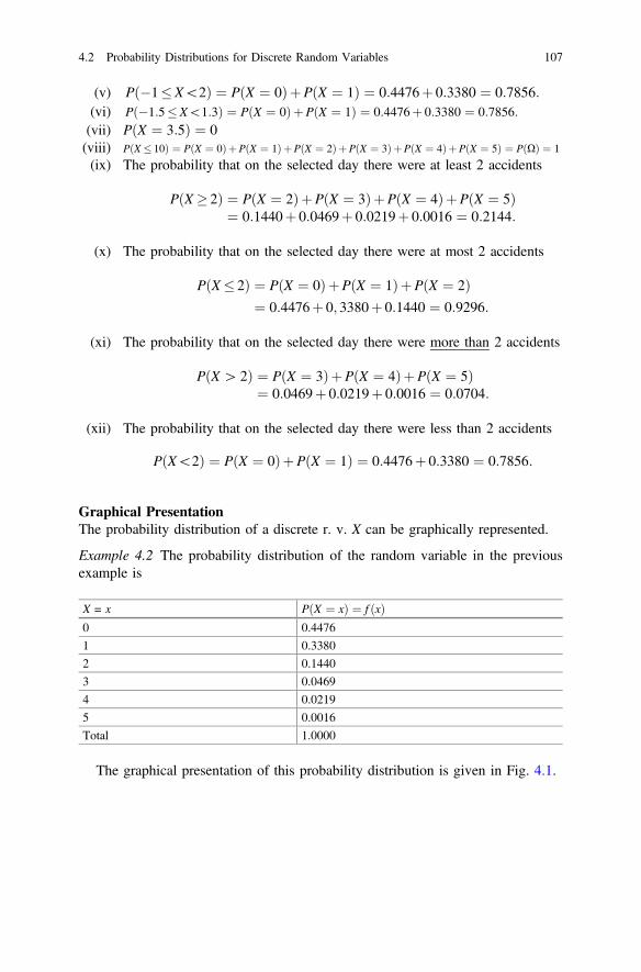
(v) P �1�X\2ð Þ ¼ P X ¼ 0ð ÞþP X ¼ 1ð Þ ¼ 0:4476þ 0:3380 ¼ 0:7856:(vi) P �1:5�X\1:3ð Þ ¼ P X ¼ 0ð ÞþP X ¼ 1ð Þ ¼ 0:4476þ 0:3380 ¼ 0:7856:(vii) PðX ¼ 3:5Þ ¼ 0(viii) P X � 10ð Þ ¼ PðX ¼ 0ÞþPðX ¼ 1ÞþPðX ¼ 2ÞþPðX ¼ 3ÞþPðX ¼ 4ÞþPðX ¼ 5Þ ¼ P Xð Þ ¼ 1
(ix) The probability that on the selected day there were at least 2 accidents
P X � 2ð Þ ¼ P X ¼ 2ð ÞþP X ¼ 3ð ÞþP X ¼ 4ð ÞþP X ¼ 5ð Þ¼ 0:1440þ 0:0469þ 0:0219þ 0:0016 ¼ 0:2144:
(x) The probability that on the selected day there were at most 2 accidents
P X� 2ð Þ ¼ P X ¼ 0ð ÞþP X ¼ 1ð ÞþP X ¼ 2ð Þ¼ 0:4476þ 0; 3380þ 0:1440 ¼ 0:9296:
(xi) The probability that on the selected day there were more than 2 accidents
P X[ 2ð Þ ¼ P X ¼ 3ð ÞþP X ¼ 4ð ÞþP X ¼ 5ð Þ¼ 0:0469þ 0:0219þ 0:0016 ¼ 0:0704:
(xii) The probability that on the selected day there were less than 2 accidents
P X\2ð Þ ¼ P X ¼ 0ð ÞþP X ¼ 1ð Þ ¼ 0:4476þ 0:3380 ¼ 0:7856:
Graphical PresentationThe probability distribution of a discrete r. v. X can be graphically represented.
Example 4.2 The probability distribution of the random variable in the previousexample is
X = x PðX ¼ xÞ ¼ f ðxÞ0 0.4476
1 0.3380
2 0.1440
3 0.0469
4 0.0219
5 0.0016
Total 1.0000
The graphical presentation of this probability distribution is given in Fig. 4.1.
4.2 Probability Distributions for Discrete Random Variables 107

4.3 Expected Value and Variance of a Discrete RandomVariable
The population mean and variance are introduced in Chap. 2. It is shown in Chap. 2that if we use all the population values, then the population mean and variance canbe defined. In this section, the population mean and variance are defined usingcorresponding probabilities of a variable. The population mean is defined as theexpected value of a variable and it can be expressed as follows:
The population mean or expected value of a discrete random variable X isdenoted by l or lX and it is defined by
EðXÞ ¼ l ¼Xx
x P X ¼ xð Þ:
Similarly, the population variance of a discrete random variable X is denoted byr2 or r2X and it is defined by
Fig. 4.1 Figure displaying probabilities of number of accidents
108 4 Probability Distributions: Discrete

VarðXÞ ¼ EðX � lÞ2 ¼ r2 ¼Xx
ðx� lÞ2P X ¼ xð Þ:
An alternative expression for the variance of a variable, X, is
VarðXÞ ¼ EðX � lÞ2 ¼ r2 ¼ EðX2Þ � EðXÞ½ �2;
where
EðXÞ ¼ l and EðX2Þ ¼Xx
x2PðX ¼ xÞ:
Example 4.3 We wish to calculate the mean l and the variance r2 of the discreterandom variable X whose probability distribution is given by the following table:
x P X ¼ xð Þ0 0.05
1 0.25
2 0.45
3 0.25
SolutionX P X ¼ xð Þ x P X ¼ xð Þ ðx� lÞ ðx� lÞ2 ðx� lÞ2
PðX ¼ xÞ0 0.05 0 −1.9 3.61 0.1805
1 0.25 0.25 −0.9 0.81 0.2025
2 0.45 0.9 0.1 0.01 0.0045
3 0.25 0.75 1.1 1.21 0.3025
Total l ¼P x P X ¼ xð Þ ¼ 1:9 r2 ¼P ðx� lÞ2PðX ¼ xÞ ¼ 0:69
l ¼Xx
x P X ¼ xð Þ ¼ 0ð Þ 0:05ð Þþ 1ð Þ 0:25ð Þþ 2ð Þ 0:45ð Þþ 3ð Þ 0:25ð Þ ¼ 1:9
r2 ¼Xx
ðx� 1:9Þ2 P X ¼ xð Þ
¼ 0� 1:9ð Þ2 0:05ð Þþ 1� 1:9ð Þ2 0:25ð Þþ 2� 1:9ð Þ2 0:45ð Þþ 3� 1:9ð Þ2 0:25ð Þ¼ 0:69:
4.3 Expected Value and Variance of a Discrete Random Variable 109
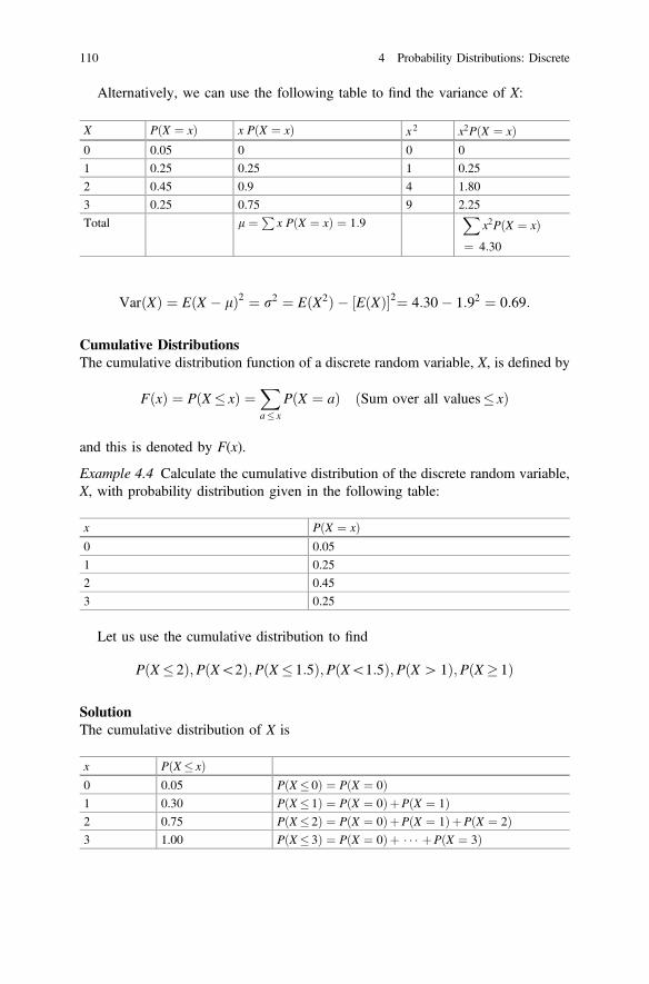
Alternatively, we can use the following table to find the variance of X:
X P X ¼ xð Þ x P X ¼ xð Þ x 2 x2PðX ¼ xÞ0 0.05 0 0 0
1 0.25 0.25 1 0.25
2 0.45 0.9 4 1.80
3 0.25 0.75 9 2.25
Total l ¼P x P X ¼ xð Þ ¼ 1:9X
x2PðX ¼ xÞ¼ 4:30
VarðXÞ ¼ EðX � lÞ2 ¼ r2 ¼ EðX2Þ � EðXÞ½ �2¼ 4:30� 1:92 ¼ 0:69:
Cumulative DistributionsThe cumulative distribution function of a discrete random variable, X, is defined by
FðxÞ ¼ P X � xð Þ ¼Xa� x
P X ¼ að Þ ðSum over all values� xÞ
and this is denoted by F(x).
Example 4.4 Calculate the cumulative distribution of the discrete random variable,X, with probability distribution given in the following table:
x P X ¼ xð Þ0 0.05
1 0.25
2 0.45
3 0.25
Let us use the cumulative distribution to find
PðX� 2Þ;P X\2ð Þ;PðX � 1:5Þ;P X\1:5ð Þ;P X[ 1ð Þ;PðX � 1Þ
SolutionThe cumulative distribution of X is
x P X� xð Þ0 0.05 P X� 0ð Þ ¼ P X ¼ 0ð Þ1 0.30 P X� 1ð Þ ¼ P X ¼ 0ð ÞþP X ¼ 1ð Þ2 0.75 P X� 2ð Þ ¼ P X ¼ 0ð ÞþP X ¼ 1ð ÞþP X ¼ 2ð Þ3 1.00 P X� 3ð Þ ¼ P X ¼ 0ð Þþ � � � þP X ¼ 3ð Þ
110 4 Probability Distributions: Discrete

Using the cumulative distribution, the probabilities are
PðX� 2Þ ¼ 0:75
P X\2ð Þ ¼ PðX� 1Þ ¼ 0:30
PðX � 1:5Þ ¼ PðX� 1Þ ¼ 0:30
PðX\1:5Þ ¼ PðX� 1Þ ¼ 0:30
PðX[ 1Þ ¼ 1� P ðX[ 1Þ� �
¼ 1� PðX� 1Þ ¼ 1� 0:30 ¼ 0:70
PðX� 1Þ ¼ 1� P ðX� 1Þ� �
¼ 1� PðX\1Þ ¼ 1� PðX� 0Þ¼ 1� 0:05 ¼ 0:95:
Example 4.5 Let us consider the following probability distribution for the variableX = number of children died to a mother in a village community from hypotheticalrelative frequencies.
x Frequency P(X = x)Relative frequency
0 79 0.65
1 27 0.22
2 10 0.08
3 4 0.03
4 2 K
Total 122 1
(a) Find the value of K.(b) Find the following probabilities:
1. P(X < 3)2. P(X � 3)3. P(X < 5)4. P(X < 1)5. P(X = 3.5)
(c) Find the probability that a mother has lost at least two children.(d) Find the probability that a mother has lost at most two children.(e) Find the expected number of children died.(f) Find the variance of X.
4.3 Expected Value and Variance of a Discrete Random Variable 111
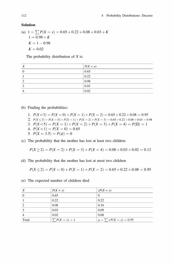
Solution
(a) 1 ¼PPðX ¼ xÞ ¼ 0:65þ 0:22þ 0:08þ 0:03þK1 ¼ 0:98þK
K ¼ 1� 0:98
K ¼ 0:02
The probability distribution of X is:
X P(X = x)
0 0.65
1 0.22
2 0.08
3 0.03
4 0.02
(b) Finding the probabilities:
1. PðX\3Þ ¼ PðX ¼ 0ÞþPðX ¼ 1ÞþPðX ¼ 2Þ ¼ 0:65þ 0:22þ 0:08 ¼ 0:952. PðX� 3Þ ¼ PðX ¼ 0ÞþPðX ¼ 1ÞþPðX ¼ 2ÞþPðX ¼ 3Þ ¼ 0:65þ 0:22þ 0:08þ 0:03 ¼ 0:98
3. PðX\5Þ ¼ PðX ¼ 1ÞþPðX ¼ 2ÞþPðX ¼ 3ÞþPðX ¼ 4Þ ¼ PðXÞ ¼ 14. PðX\1Þ ¼ PðX ¼ 0Þ ¼ 0:655. PðX ¼ 3:5Þ ¼ Pð/Þ ¼ 0
(c) The probability that the mother has lost at least two children
PðX � 2Þ ¼ PðX ¼ 2ÞþPðX ¼ 3ÞþPðX ¼ 4Þ ¼ 0:08þ 0:03þ 0:02 ¼ 0:13
(d) The probability that the mother has lost at most two children
PðX � 2Þ ¼ PðX ¼ 0ÞþPðX ¼ 1ÞþPðX ¼ 2Þ ¼ 0:65þ 0:22þ 0:08 ¼ 0:95
(e) The expected number of children died
X P(X = x) xP(X = x)
0 0.65 0
1 0.22 0.22
2 0.08 0.16
3 0.03 0.09
4 0.02 0.08
TotalP
PðX ¼ xÞ ¼ 1 l ¼P x PðX ¼ xÞ ¼ 0:55
112 4 Probability Distributions: Discrete
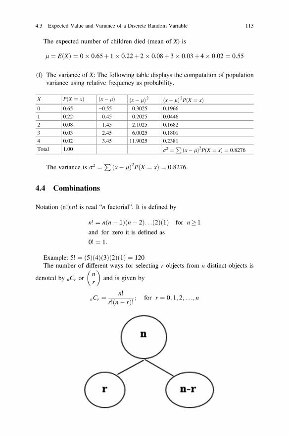
The expected number of children died (mean of X) is
l ¼ EðXÞ ¼ 0� 0:65þ 1� 0:22þ 2� 0:08þ 3� 0:03þ 4� 0:02 ¼ 0:55
(f) The variance of X: The following table displays the computation of populationvariance using relative frequency as probability.
X P X ¼ xð Þ ðx� lÞ ðx� lÞ 2 ðx� lÞ 2PðX ¼ xÞ0 0.65 −0.55 0.3025 0.1966
1 0.22 0.45 0.2025 0.0446
2 0.08 1.45 2.1025 0.1682
3 0.03 2.45 6.0025 0.1801
4 0.02 3.45 11.9025 0.2381
Total 1.00 r2 ¼P ðx� lÞ2PðX ¼ xÞ ¼ 0:8276
The variance is r2 ¼P ðx� lÞ2PðX ¼ xÞ ¼ 0:8276:
4.4 Combinations
Notation (n!):n! is read “n factorial”. It is defined by
n! ¼ n n� 1ð Þ n� 2ð Þ. . . 2ð Þ 1ð Þ for n� 1
and for zero it is defined as
0! ¼ 1:
Example: 5! ¼ ð5Þð4Þð3Þð2Þð1Þ ¼ 120The number of different ways for selecting r objects from n distinct objects is
denoted by nCr ornr
� �and is given by
nCr ¼ n!r! n� rð Þ! ; for r ¼ 0; 1; 2; . . .; n
4.3 Expected Value and Variance of a Discrete Random Variable 113

Notes:
1. nCr is read as “n” choose “r”.2. nCn ¼ 1; nC0 ¼ 1;3. nCr ¼ nCn�r (for example: 10C3 ¼ 10C7
4. nCr = number of unordered subsets of a set of (n) objects such that each subsetcontains (r) objects.
Example 4.6 For n = 4 and r = 2,
4C2 ¼ 4!2! 4� 2ð Þ! ¼
4!2!� 2!
¼ 4� 3� 2� 1ð2� 1Þ � ð2� 1Þ ¼ 6
4C2 = 6 = the number of different ways for selecting 2objects from 4 distinct objects.
Example 4.7 Suppose that we have the set {a, b, c, d} of (n = 4) objects.We wish to choose a subset of two objects. The possible subsets of this set with
two elements in each subset are
fa; bg; fa; cg; fa; dg; fb; dg; fb; cg; fc; dg
The number of these subsets is 4C2 ¼ 6:
4.5 Bernoulli Distribution
The Bernoulli distribution arises from a trial with two possible outcomes which aretermed traditionally as success or failure. Each trial with two outcomes may beconsidered as a Bernoulli trial. The probabilities of success or failure are comple-mentary to each other so that if the probability of success is denoted by p then theprobability of failure is 1 − p, where p satisfies 0� p� 1. One very familiarexample is if we randomly draw an individual then the selected individual may ormay not suffer from a disease at the time of survey with probability p of sufferingfrom the disease and with probability 1 − p = q of not suffering from the disease. Inthat case, p + q = 1. A Bernoulli process consists of n repeated Bernoulli trialswhere trials are independent with a constant probability of success, p. The Bernoullidistribution plays a very important role in biostatistics and epidemiology.
The Bernoulli variable, X, is a binary variable with discrete probability massfunction as shown below
f ðx; pÞ ¼ PðX ¼ xÞ ¼ pxð1� pÞ1�x for x = 0,10 otherwise:
�
114 4 Probability Distributions: Discrete
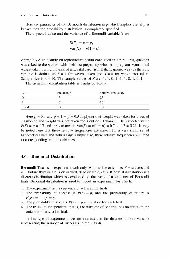
Here the parameter of the Bernoulli distribution is p which implies that if p isknown then the probability distribution is completely specified.
The expected value and the variance of a Bernoulli variable X are
EðXÞ ¼ l ¼ p;
VarðXÞ ¼ pð1� pÞ:
Example 4.8 In a study on reproductive health conducted in a rural area, questionwas asked to the women with their last pregnancy whether a pregnant woman hadweight taken during the time of antenatal care visit. If the response was yes then thevariable is defined as X = 1 for weight taken and X = 0 for weight not taken.Sample size is n = 10. The sample values of X are: 1, 1, 0, 1, 1, 1, 0, 1, 0, 1.
The frequency distribution table is displayed below
X Frequency Relative frequency
0 3 0.3
1 7 0.7
Total 10 1.0
Here p = 0.7 and q = 1 − p = 0.3 implying that weight was taken for 7 out of10 women and weight was not taken for 3 out of 10 women. The expected valueE(X) = p = 0.7 and the variance is Var(X) = p(1 − p) = 0.7 � 0.3 = 0.21. It maybe noted here that these relative frequencies are shown for a very small set ofhypothetical data and with a large sample size, these relative frequencies will tendto corresponding true probabilities.
4.6 Binomial Distribution
Bernoulli Trial is an experiment with only two possible outcomes: S = success andF = failure (boy or girl, sick or well, dead or alive, etc.). Binomial distribution is adiscrete distribution which is developed on the basis of a sequence of Bernoullitrials. Binomial distribution is used to model an experiment for which:
1. The experiment has a sequence of n Bernoulli trials.2. The probability of success is PðSÞ ¼ p, and the probability of failure is
PðFÞ ¼ 1� p ¼ q.3. The probability of success PðSÞ ¼ p is constant for each trial.4. The trials are independent, that is, the outcome of one trial has no effect on the
outcome of any other trial.
In this type of experiment, we are interested in the discrete random variablerepresenting the number of successes in the n trials.
4.5 Bernoulli Distribution 115

Let X = number of successes in the n trials, then the possible values ofX (number of success in n trails) are x = 0, 1, 3, …, n.
The random variable, X, has a binomial distribution with parameters n and p, andwe write X�Binomialðn; pÞ.
The probability distribution of X is given by
P X ¼ xð Þ ¼ nCxpxqn�x for x ¼ 0; 1; 2; . . .; n0 otherwise
�;
where nCx ¼ n!x! n�xð Þ!.
We can write the probability distribution of X as displayed in the following table:
X PðX ¼ xÞ0 nC0 p0 qn�0 ¼ qn
1 nC1 p1 qn�1
2 nC2 p2 qn�2
..
. ...
n- 1 nCn�1 pn�1 q1
n nCn pn q0 ¼ pn
Total 1
The Expected Value and the Variance of a Binomial Variable XIf X * Binomial(n, p), then using expectations defined in the previous section, theexpected value and the variance of a binomial variable X can be obtained.
The expected value or mean is EðXÞ ¼ l ¼ np and the variance isVarðXÞ ¼ EðX � lÞ2 ¼ r2 ¼ npq.
Example 4.9 Suppose that the probability that an adult person is suffering fromdiabetes in a population is 0.10. Suppose that we randomly select a sample of 6persons.
(1) Find the probability distribution of the random variable (X) representing thenumber of persons with diabetes in the sample.
(2) Find the expected number of persons with diabetes in the sample (mean of X).(3) Find the variance of X.(4) What is the probability that there will be exactly two persons with diabetes?(5) What is the probability that there will be at most two persons with diabetes?(6) What is the probability that there will be at least four persons with diabetes?
SolutionWe are interested in the following random variable:
X = the number of persons with diabetes in the sample of six persons.
116 4 Probability Distributions: Discrete

Notes:
(i) Bernoulli trial: diagnosing whether a person has diabetes or not. There aretwo outcomes for each trial, diabetic (S) or nondiabetic (F).
(ii) Number of trials = 6 or n = 6.(iii) Probability of success: PðSÞ ¼ p ¼ 0:10:(iv) Probability of failure: PðFÞ ¼ q ¼ 1� p ¼ 0:9.(v) The trials are independent because of the fact that the result of each person
does not affect the result of any other person since the selection was made atrandom.
The random variable, X, has a binomial distribution with parameters: n = 6 andp = 0.10, that is X * Binomial (6, 0.10).
The possible values of X are X = x, where
x ¼ 0; 1; 2; 3; 4; 5; 6:
(1) The probability distribution of X is
P X ¼ xð Þ ¼ 6Cx 0:1ð Þx 0:9ð Þ6�x; x ¼ 0; 1; 2; 3; 4; 5; 60; otherwise:
�
The probabilities of all values of X are
P X ¼ 0ð Þ ¼ 6C0 0:1ð Þ0 0:9ð Þ6¼ 1ð Þ 0:1ð Þ0 0:9ð Þ6¼ 0:531441
P X ¼ 1ð Þ ¼ 6C1 0:1ð Þ1 0:9ð Þ5¼ 6ð Þ 0:1ð Þ 0:9ð Þ5¼ 0:354294
P X ¼ 2ð Þ ¼ 6C2 0:1ð Þ2 0:9ð Þ4¼ 15ð Þ 0:1ð Þ2 0:9ð Þ4¼ 0:098415
P X ¼ 3ð Þ ¼ 6C3 0:1ð Þ3 0:9ð Þ3¼ 20ð Þ 0:1ð Þ3 0:9ð Þ3¼ 0:014580
P X ¼ 4ð Þ ¼ 6C4 0:1ð Þ4 0:9ð Þ2¼ 15ð Þ 0:1ð Þ4 0:9ð Þ2¼ 0:001215
P X ¼ 5ð Þ ¼ 6C5 0:1ð Þ5 0:9ð Þ1¼ 6ð Þ 0:1ð Þ5 0:9ð Þ1¼ 0:000054
P X ¼ 6ð Þ ¼ 6C6 0:1ð Þ6 0:9ð Þ0¼ 1ð Þ 0:1ð Þ6 1ð Þ ¼ 0:000001
The probability distribution of X can be presented by the following table:
X PðX ¼ xÞ0 0.531441
1 0.354294
2 0.098415
3 0.01458
4 0.001215
5 0.000054
6 0.000001
4.6 Binomial Distribution 117

The probability distribution of X can be presented by the following graph(Fig. 4.2):
(2) The mean of the distribution (the expected number of men out of 6 withdiabetes) is
l ¼ np ¼ ð6Þð0:1Þ ¼ 0:6:
(3) The variance is
r2 ¼ npq ¼ ð6Þð0:1Þð0:9Þ ¼ 0:54:
(4) The probability that there will be exactly two men with diabetes is
PðX ¼ 2Þ ¼ 0:098415:
Fig. 4.2 Figure displaying binomial probabilities
118 4 Probability Distributions: Discrete

(5) The probability that there will be at most two men with diabetes is
PðX� 2Þ ¼ PðX ¼ 0ÞþPðX ¼ 1ÞþPðX ¼ 2Þ¼ 0:531441þ 0:354294þ 0:098415
¼ 0:98415:
(6) The probability that there will be at least four men with diabetes is
PðX� 4Þ ¼ P X ¼ 4ð ÞþP X ¼ 5ð ÞþP X ¼ 6ð Þ¼ 0:001215þ 0:000054þ 0:000001
¼ 0:00127:
Example 4.10 An experiment is conducted to select a sample of five patientsadmitted to the emergency care in a hospital randomly. Let the probability ofselecting a patient with diabetes-related complications is 0.25. Here, the variableX denotes the number of patients admitted to the emergency care withdiabetes-related complications. Then some of the typical questions relevant to thestudy can be outlined as follows:
(a) Find the probability distribution of X.(b) Find the probability that at least two patients have diabetes-related
complications.(c) Find the probability that at most three patients have diabetes-related
complications.(d) Find the expected number of patients with diabetes-related complications.(e) Find the variance of the number of patients with diabetes-related complications
out of the five patients.
SolutionX = the number of patients out of five with diabetes-related complications
The Bernoulli trial is the process of diagnosing the person with diabetes-relatedcomplications with
p = probability of selecting a patient in emergency care with diabetes-relatedcomplications,
q = 1 − p = probability of selecting a patient in emergency care withoutdiabetes-related complications.
Here, n ¼ 5 ¼ number of patients selected randomly;
p ¼ 0:25;
q ¼ 1� p ¼ 0:75:
4.6 Binomial Distribution 119

(a) X has a binomial distribution Binomial distribution with parameter n ¼ 5 andp ¼ 0:25 or X �Binomial 5; 0:25ð Þ:The possible values of X = x are x = 0, 1, 2, 3, 4, 5.The probability distribution is
P X ¼ xð Þ ¼ nCxpxqn�x; for x ¼ 0; 1; 2; . . .; n
0; otherwise
�
P X ¼ xð Þ ¼ 5Cxð0:25Þxð0:75Þ5�x; for x ¼ 0; 1; 2; 3; 4; 5
0; otherwise
(
X P(X = x)
0 5C0 � 0:250 � 0:755�0 ¼ 0:23730
1 5C1 � 0:251 � 0:755�1 ¼ 0:39551
2 5C2 � 0:252 � 0:755�2 ¼ 0:26367
3 5C3 � 0:253 � 0:755�3 ¼ 0:08789
4 5C4 � 0:254 � 0:755�4 ¼ 0:01465
5 5C5 � 0:255 � 0:755�5 ¼ 0:00098
TotalP
PðX ¼ xÞ ¼ 1
(b) The probability that at least two patients have diabetes-related complications is
PðX � 2Þ ¼ P X ¼ 2ð ÞþP X ¼ 3ð ÞþP X ¼ 4ð ÞþP X ¼ 5ð Þ¼ 0:26367þ 0:08789þ 0:01465þ 0:00098
¼ 0:36719:
(c) The probability that at most three patients have diabetes-related complications is
PðX � 3Þ ¼ P X ¼ 0ð ÞþP X ¼ 1ð ÞþP X ¼ 2ð ÞþP X ¼ 3ð Þ¼ 0:23730þ 0:39551þ 0:26367þ 0:08789
¼ 0:98437:
(d) The expected number of patients with diabetes-related complications out of thefive patients is
l ¼ np ¼ 5� 0:25 ¼ 1:25:
(e) The variance of the number of patients with diabetes-related complications is
r2 ¼ n pq ¼ 5� 0:25� 0:75 ¼ 0:93750:
120 4 Probability Distributions: Discrete
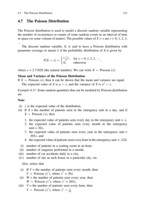
4.7 The Poisson Distribution
The Poisson distribution is used to model a discrete random variable representingthe number of occurrences or counts of some random events in an interval of timeor space (or some volume of matter). The possible values of X = x are x = 0, 1, 2, 3,…
The discrete random variable, X, is said to have a Poisson distribution withparameter (average or mean) k if the probability distribution of X is given by
P X ¼ xð Þ ¼ e�kkx
x! ; for x ¼ 0; 1; 2; 3; . . .0; otherwise
�;
where e = 2.71828 (the natural number). We can write X * Poisson (k).
Mean and Variance of the Poisson DistributionIf X * Poisson (k), then it can be shown that the mean and variance are equal.
The expected value of X is l ¼ k, and the variance of X is r2 ¼ k.
Example 4.11 Some random quantities that can be modeled by Poisson distributionare
Note:
(i) k is the expected value of the distribution.(ii) If X = the number of patients seen in the emergency unit in a day, and if
X * Poisson (k), then
1. the expected value of patients seen every day in the emergency unit = k,2. the expected value of patients seen every month in the emergency
unit = 30k,3. the expected value of patients seen every year in the emergency unit =
365k, and4. the expected value of patients seen every hour in the emergency unit = k/24.
(i) number of patients in a waiting room in an hour,(ii) number of surgeries performed in a month,(iii) number of car accidents daily in a city,(iv) number of rats in each house in a particular city, etc.
Also, notice that
(i) If Y = the number of patients seen every month, thenY * Poisson (k*), where k* = 30k.
(ii) W = the number of patients seen every year, thenW * Poisson (k*), where k* = 365k,
(iii) V = the number of patients seen every hour, thenV * Poisson (k*), where k ¼ k
24.
4.7 The Poisson Distribution 121
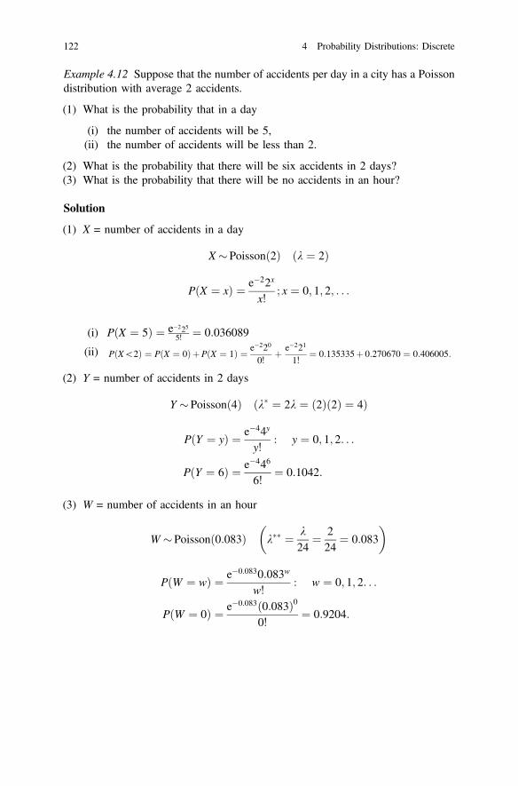
Example 4.12 Suppose that the number of accidents per day in a city has a Poissondistribution with average 2 accidents.
(1) What is the probability that in a day
(i) the number of accidents will be 5,(ii) the number of accidents will be less than 2.
(2) What is the probability that there will be six accidents in 2 days?(3) What is the probability that there will be no accidents in an hour?
Solution
(1) X = number of accidents in a day
X� Poissonð2Þ ðk ¼ 2Þ
P X ¼ xð Þ ¼ e�22x
x!; x ¼ 0; 1; 2; . . .
(i) P X ¼ 5ð Þ ¼ e�2255! ¼ 0:036089
(ii) P X\2ð Þ ¼ P X ¼ 0ð ÞþP X ¼ 1ð Þ ¼ e�220
0!þ e�221
1!¼ 0:135335þ 0:270670 ¼ 0:406005:
(2) Y = number of accidents in 2 days
Y � Poissonð4Þ k ¼ 2k ¼ ð2Þð2Þ ¼ 4ð Þ
P Y ¼ yð Þ ¼ e�44y
y!: y ¼ 0; 1; 2. . .
P Y ¼ 6ð Þ ¼ e�446
6!¼ 0:1042:
(3) W = number of accidents in an hour
W � Poisson 0:083ð Þ k ¼ k24
¼ 224
¼ 0:083� �
P W ¼ wð Þ ¼ e�0:0830:083w
w!: w ¼ 0; 1; 2. . .
P W ¼ 0ð Þ ¼ e�0:083 0:083ð Þ00!
¼ 0:9204:
122 4 Probability Distributions: Discrete

Poisson Approximation for Binomial DistributionSuppose that the random variable X has a binomial distribution with parametern and p, that is X * binomial (n, p). If the number of trial is large (n ! ∞), andthe probability of success is small (p ! 0), and the quantity l = np remainsconstant, then the binomial distribution, binomial (n, p), can approximated byPoisson distribution Poisson(l), where l ¼ np. That is, for large n and small p wehave
Binomial (n, p) Poisson(l)
nx
� �pxð1� pÞn�x e�llx
x!; x ¼ 0; 1; . . .; n;
where l = np.
Example 4.13 Let us consider that X has a binomial distribution with parametersn = 5000 and p = 0.002. The probability that the number of success is less than orequal to 5 or P(X � 5) can be obtained as follows.
Solution
(a) The probability of number of success less than or equal to 5 for X * binomial(5000, 0.002):
PðX� 5Þ ¼X5x¼0
5000x
� �ð0:002Þxð0:998Þ5000�x ¼ 0:0669
(b) We can use the Poisson approximation of binomial for this problem becausen = 5000 is quite large and p = 0.002 is very small.
We can approximate the mean for Poisson distribution by the followingrelationship:
l ¼ np ¼ 5000� 0:002 ¼ 10:
Using this as the parameter of the Poisson distribution as an approximation forbinomial, we obtain the probability of less than or equal to 5 for with parameterl = 10, i.e., X * Poisson(10).
PðX� 5Þ ¼X5x¼0
e�1010x
x!¼ 0:0671:
We observe that the approximation is quite satisfactory.
4.7 The Poisson Distribution 123

4.8 Geometric Distribution
In an experiment, if we are interested in the random variable, X, representing thetotal number of trials required in order to obtain the success for the first time afterX − 1 failures, then it follows a geometric distribution. The probability function ofthe random variable, X, is
fXðxÞ ¼ PðX ¼ xÞ ¼ pð1� pÞx�1; x ¼ 1; 2; 3; . . .0; otherwise
�
In this case, we can write X�GeometricðpÞ. The geometric distribution dependson only one parameter which is the probability of success (p). The variableX resembles in some sense incidence of disease.
Mean and Variance of the Geometric DistributionThe expected value and the variance of the geometric distribution are
lX ¼ EðXÞ ¼ 1p;
r2X ¼ VarðXÞ ¼ ð1� pÞp2
:
Example 4.14 Let us consider a hypothetical follow-up study on incidence of heartdisease. The study is continued until the incidence of heart disease is diagnosedstarting with no heart disease at the beginning of the study. Once an individual inthe sample is diagnosed with heart disease, the number of follow-ups required is thevariable X. We want to find the probability that the researcher needs to continue forfour follow-ups to find an incidence case of heart disease. Let us assume that theprobability of an incidence case is 0.3.
SolutionLet X be the random variable representing the number of follow-ups required todiagnose the incidence of heart disease. The random variable, X has a geometricdistribution with parameter p ¼ 0:3 that is
X�GeometricðpÞ ¼ Geometricð0:30Þ:The probability function is
fXðxÞ ¼ PðX ¼ xÞ ¼ 0:30� 0:7x�1; x ¼ 1; 2; 3; . . .0; otherwise:
�
124 4 Probability Distributions: Discrete

The probability that four follow-ups will be necessary to find an incidence caseof heart disease at the fourth follow-up is
PðX ¼ 4Þ ¼ 0:3� ð0:7Þ3 ¼ 0:1029:
4.9 Multinomial Distribution
The multinomial distribution is a generalization of the binomial distribution. As wehave mentioned earlier, Bernoulli trial is an experiment that can have only twooutcomes (either success or failure) and a binomial random variable is the number oftimes of obtaining the outcome of success when we independently perform theBernoulli trial n times. Analogically, a multinomial trial is an experiment that canhave k outcomes (say: A1;A2; . . .;Ak). It is assumed that the probability of the ithoutcome ðAiÞ is pi ¼ PðAiÞ, where ði ¼ 1; 2; . . .; kÞ, andPk
i¼1 pi ¼Pk
i¼1 PðAiÞ ¼ 1.Now, suppose that we independently repeat performing a multinomial trial
n times with the probabilities ðp1; p2; . . .; pkÞ being constant in each trial, and let usdefine the random variable Xi to be the number of times we obtain the ith outcomeðAiÞ. In this case, the random vector ðX1;X2; . . .;XkÞ follows a multinomial dis-tribution with parameters ðn; p1; p2; . . .; pkÞ, and the probability function of thismultinomial distribution is:
P X1 ¼ x1;X2 ¼ x2; . . .;Xk ¼ xkð Þ ¼n!
x1!x2!...xk !px11 p
x22 . . .p
xkk ; when
Pki¼1 xi ¼ n
0; otherwise:
�
Some Notes
1. The event X1 ¼ x1;X2 ¼ x2; . . .;Xk ¼ xkð Þ means that the outcome ðA1Þ occursðx1Þ times, the outcome ðA2Þ occurs ðx2Þ times, …, and the outcome ðAkÞ occursðxkÞ times when we independently repeat performing the multinomial trial(n) times.
2. 0� pi � 13.Pk
i¼1 pi ¼Pk
i¼1 PðAiÞ ¼ 1
4.Pk
i¼1 xi ¼ n5. The value of one of the variables ðX1;X2; . . .;XkÞ can be determined by the
values of the other variables, for example, x1 ¼ n�Pki¼2 xi.
6. The random variable Xi follows a binomial distribution with parameters ðn; piÞ.7. The mean of Xi is npi.8. The variance of Xi is npið1� piÞ.
4.8 Geometric Distribution 125

Example 4.15 Suppose that we have conducted a study on three different types ofcomplications associated with a disease. The probability of suffering from com-plication type 1 is 0.1, complication type 2 is 0.3, and complication type 3 is 0.6.Let us select 6 patients randomly. Then, the following questions are asked.
(1) What is the probability of selecting 2, 1, and 3 patients with complication types1, 2, and 3 respectively?
(2) What is the expected number of patients with complication type 2 in thesample?
SolutionThe trial is the procedure of selecting six patients with complication types 1, 2, and3. Let A1 = complication type 1, A2 = complication type 2, A3 = complication type3. The experiment is comprised of n = 6 trials. Then the probabilities of compli-cation types are
p1 ¼ PðA1Þ ¼ P complication type 1ð Þ ¼ 0:1;
p2 ¼ PðA2Þ ¼ P complication type 2ð Þ ¼ 0:3; and
p3 ¼ PðA3Þ ¼ P complication type 3ð Þ ¼ 0:6:
Let us define X1 = number of patients with complication type 1, X2 = number ofpatients with complication type 2 and X3 = number of patients with complicationtype 3. The random vector (X1;X2;X3) follows a multinomial distribution withparameters ðn ¼ 6; p1 ¼ 0:1; p2 ¼ 0:3; p3 ¼ 0:6Þ.(1) The event ðX1 ¼ 2;X2 ¼ 1;X3 ¼ 3Þ = the event of getting 2 with complication
type 1, 1 with complication type 2 and 3 with complication type 3. The cor-responding multinomial probability is
PðX1 ¼ 2;X2 ¼ 1;X3 ¼ 3Þ ¼ 6!2!� 1!� 3!
0:12 � 0:31 � 0:63 ¼ 0:039:
(2) The expected number of patients with type 2 complication in the sample = theexpected value of X2 ¼ np2 ¼ 6� 0:3 ¼ 1:8.
4.10 Hypergeometric Distribution
Let us consider a population with two types of elements (or 2 categories). Eachelement in the population can be classified as first type (success) or second type(failure). Let us define the following quantities: N = population size, K = numberof elements of the first type in the population and N − K = number of elements ofthe second type in the population. Suppose that we select a sample of n elements atrandom from this population, and define the random variable, X, to be the number
126 4 Probability Distributions: Discrete

of elements of first type (number of successes) in the sample. We are interested infinding the probability distribution of X.
To find the probability distribution of X, we should distinguish between twocases since there are two methods of selection, which are selection with replace-ment and selection without replacement.
(1) Case 1: If we select the elements of the sample at random and with replacement(i.e., each selected element is replaced back to the population before the nextselection), then
X �Binomial n; pð Þ
where p ¼ KN.
(2) Second case: suppose that we select the elements of the sample at random andwithout replacement (i.e., each selected element is removed from the populationbefore the next selection). When the selection is made without replacement, therandom variable X has a hypergeometric distribution with parameters N, n, andK, and we write X * h(N, n, K).
The probability distribution of X is given by
f ðxÞ ¼ PðX ¼ xÞ ¼ hðx;N; n;KÞ ¼
K
x
!�
N � K
n� x
!
N
n
! ; x ¼ 0; 1; 2; . . .; n;
0; otherwise:
8>>>>>><>>>>>>:
It should be noticed that the possible values of X must satisfy the followinginequalities: 0 � x � K and 0 � n − x � N − K implying 0 � x � K andn − N + K � x � n or max{0, n − N + K} � x � min{K, n}.
Mean and VarianceThe expected value and the variance of the hypergeometric distribution h(N, n,K) are
EðXÞ ¼ l ¼ n� KN;
VarðXÞ ¼ r2 ¼ n� KN� 1� K
N
� �� N � nN � 1
:
Example 4.16 Consider a hypothetical study on admission to emergency care in ahospital with acute breathing problem. During the study period, 50 patients wereadmitted, 15 males and 35 females. A sample of five patients has been selectedrandomly without replacement.
4.10 Hypergeometric Distribution 127

(1) What is the probability that exactly one male patient is found in the sample?(2) What is the expected number (mean) of males in the sample?(3) What is the variance of number of males in the sample?
SolutionThere are two types or categories male and female. Let X = number of males in thesample. We have N = 50, K = 15, and n = 5. Then X has a hypergeometric dis-tribution with parameters N = 50, n = 5, and K = 15 which can be denoted byX * h(N, n, K) = h(50, 5, 15) and the probability distribution of X is given by
f ðxÞ ¼ PðX ¼ xÞ ¼ hðx; 50; 5; 15Þ ¼
15x
� �� 35
5� x
� �505
� � ; x ¼ 0; 1; 2; . . .; 15
0; otherwise
8>>>><>>>>:
but the values of X must satisfy: 0 � x � K and n − N + K � x � n , 0� x � 15 and −30 � x � 5, hence, the probability distribution of X is given by
f ðxÞ ¼ PðX ¼ xÞ ¼ hðx; 50; 5; 15Þ ¼
15x
� �� 35
5� x
� �505
� � ; x ¼ 0; 1; 2; 3; 4; 5
0; otherwise:
8>>>><>>>>:
(1) The probability that exactly one male is found in the sample is
f 1ð Þ ¼ P X ¼ 1ð Þ ¼ h 1; 50; 5; 15ð Þ ¼151
� �� 35
5� 1
� �505
� � ¼151
� �� 35
4
� �505
� �
¼ 15� 523602118760
¼ 0:3707
(2) The expected number of males is
EðXÞ ¼ n� kN
¼ 5� 1550
¼ 1:50:
128 4 Probability Distributions: Discrete
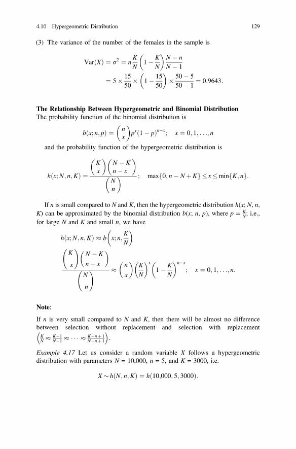
(3) The variance of the number of the females in the sample is
VarðXÞ ¼ r2 ¼ nKN
1� KN
� �N � nN � 1
¼ 5� 1550
� 1� 1550
� �� 50� 550� 1
¼ 0:9643:
The Relationship Between Hypergeometric and Binomial DistributionThe probability function of the binomial distribution is
bðx; n; pÞ ¼ nx
� �pxð1� pÞn�x; x ¼ 0; 1; . . .; n
and the probability function of the hypergeometric distribution is
hðx;N; n;KÞ ¼Kx
� �N � Kn� x
� �Nn
� � ; maxf0; n� NþKg� x�minfK; ng:
If n is small compared to N and K, then the hypergeometric distribution h(x; N, n,K) can be approximated by the binomial distribution b(x; n, p), where p ¼ K
N; i.e.,for large N and K and small n, we have
h x;N; n;Kð Þ b x; n;KN
� �K
x
!N � K
n� x
� �
N
n
! n
x
� �KN
� �x
1� KN
� �n�x
; x ¼ 0; 1; . . .; n:
Note:
If n is very small compared to N and K, then there will be almost no differencebetween selection without replacement and selection with replacementKN K�1
N�1 � � � K�nþ 1N�nþ 1
� �.
Example 4.17 Let us consider a random variable X follows a hypergeometricdistribution with parameters N = 10,000, n = 5, and K = 3000, i.e.
X� h N; n;Kð Þ ¼ h 10;000; 5; 3000ð Þ:
4.10 Hypergeometric Distribution 129

Find P(X = 2) using the exact method and binomial approximation of hyper-geometric distribution.
Solution
(1) Exact method
The exact probability using hypergeometric distribution is
PðX ¼ 2Þ ¼30002
� �70003
� �10;000
5
� � ¼ 0:3088
(2) Approximate method
Since n = 5 is small relative to N = 10000 and K = 3000, we can approximatethe hypergeometric probabilities using binomial probabilities as follows:
n ¼ 5 number of trialsð Þp ¼ K=N ¼ 3000=10000 ¼ 0:3 probability of successð Þ
X� hðx; 10000; 5; 3000Þ bðx; 5; 0:3Þ
PðX ¼ 2; 5; 0:3Þ ¼ 5
2
� �ð0:3Þ2ð0:7Þ3 ¼ 0:3087
We notice that the approximation is very good.
4.11 Negative Binomial Distribution
The negative binomial distribution is based on an experiment consisting of asequence of repeated independent Bernoulli trials. The experiment is continueduntil the rth success is obtained under the following conditions:
(i) Each trial has only two outcomes (success and failure).(ii) The trials are independent.(iii) The probability of success P(S) = p remains constant in each trial.(iv) The number of success required is r, where r is a fixed given positive integer
(r = 1, 2, …).(v) The experiment is immediately terminated once the rth success is obtained.
In the negative binomial experiment, we are interested in the random variable, X,representing the total number of trials required to obtain the first r successes for thefirst time. For example, let the experiment consists of independently continuing
130 4 Probability Distributions: Discrete

observing until r successes are observed and recording the number of trials requiredto obtain r successes.
In the negative binomial experiment, we should notice the following:
(i) the number of successes is r (fixed number),(ii) the number of trials is X (random variable),(iii) the number of failures = X − r (random),(iv) the result of the last trial (the Xth trial) is success,(v) there are r − 1 successes and X − r failures in the first X − 1 trails (the trials
before the last one),(vi) the number of trials required for obtaining the first r successes must not be
less than r (i.e., X � r),(vii) the set of possible values of X is {r, r + 1, r + 2, …}.
The probability function of the random variable, X, is
fXðxÞ ¼ PðX ¼ xÞ ¼x� 1
r � 1
!prð1� pÞx�r; x ¼ r; rþ 1; rþ 2; . . .
0; otherwise:
8><>:
In this case, we write X�NBðr; pÞ. The negative binomial distribution dependson two parameters which are the number of successes (r) and the probability ofsuccess (p). The geometric distribution is a special case of the negative binomialdistribution where r ¼ 1. We should notice that NBð1; pÞ ¼ Geometric(pÞ.Mean and VarianceThe mean (expected value) and the variance of the negative binomial distributionNBðr; pÞ are
lX ¼ EðXÞ ¼ rp;
r2X ¼ VarðXÞ ¼ rð1� pÞp2
:
Notes:
1. For the special case where r = 1, the negative binomial distribution NBð1; pÞ iscalled the geometric distribution with parameter p, and in this case, the randomvariable X �NBð1; pÞ ¼ Geometric(pÞ represents the total number of trialsrequired to obtain the first success.
2. In the case of negative binomial distribution, the number of trials is random andthe number of successes is fixed. While in the case of binomial distribution, thenumber of trials is fixed and the number of successes is random.
4.11 Negative Binomial Distribution 131

Example 4.18 Let us consider a hypothetical study on utilization of health careservices. For an elderly person, let the number of days required to make the rth visitto a community hospital is of interest. Let us also consider that the probability of avisit each time remains constant and it has been considered to be 0.4. The researcherwants to find the probability of number of days required to make the third visit sincethe start of the study. Suppose that the random variable X represents the totalnumber of days required to visit the community clinic for the third time.
(1) Find the probability distribution of X.(2) What is the expected number (mean) of days required for an elderly to visit the
community clinic for the third time?(3) What is the probability that 10 days will be needed to make the third visit to the
community clinic?
Solution
(1) The random variable, X has a negative binomial distribution with parameters:r ¼ 3 and p ¼ 0:4, that is
X �NBðr; pÞ ¼ NBð3; 0:4Þ:
The probability function is
PðX ¼ xÞ ¼x� 12
� �� 0:43 � 0:6x�3; x ¼ 3; 4; 5; . . .
0; otherwise:
8<:
(2) The expected number (mean) of days required to make the third visit is
lX ¼ EðXÞ ¼ rp¼ 3
0:4¼ 7:5:
(3) The probability that the researcher will have to wait for ten days to observe thethird visit to the community clinic is
PðX ¼ 10Þ ¼ 9
2
!0:43ð0:6Þ7 ¼ 0:0645:
The negative binomial distribution provides answers to very useful questionsregarding count data. The geometric distribution is a special case of the negativebinomial distribution for r = 1. Sometimes, the negative binomial distribution isused as an alternative to the Poisson distribution if there is overdispersion in thedata. As we know that in case of the Poisson distribution, there is equality of meanand variance which may not represent some count data in reality where the varianceis greater than the mean resulting in overdispersion. The negative binomial distri-bution can be employed to analyze such data instead of the Poisson distribution.
132 4 Probability Distributions: Discrete

4.12 Summary
The discrete probability distributions are introduced in this chapter. The generalrules of discrete probability distributions are illustrated and the concepts ofexpected value and variance are shown. The rules are illustrated with a number ofexamples. This chapter includes brief introduction of the Bernoulli distribution,binomial distribution, Poisson distribution, geometric distribution, multinomialdistribution, hypergeometric distribution, and negative binomial distribution. Theimportant properties of these distributions are discussed and illustrated withexamples. The applications of these useful distributions are given high priority inillustrations.
Exercises
4:1 Suppose that X be a discrete random variable with the following probabilitydistribution:
X PðX ¼ xÞ0 K
1 0.2
2 0.3
3 0.2
4 0.1
Find the following:
(i) the value of k;(ii) the expected value of X;(iii) the expected value of X2;(iv) the variance of X;(v) the cumulative probability distribution of X;(vi) PðX � 2Þ;(vii) PðX[ 2Þ:
4:2 The following probability distribution represents probability of X = numberof complications a person suffers at old age in a community.
X 0 1 2 3 4 5
P(x) 0.01 0.09 0.15 0.40 0.25 0.10
4.12 Summary 133

Find the probability that the number of complications is
(a) 0;(b) more than 2;(c) more than or equal to 3;(d) 1�X � 3:
4:3 Suppose a diagnostic test conducted on five persons. The purpose is todetermine probability of x, the number who suffer from a certain disease.Suppose that 20% of all the individuals suffer from the disease. Then find
(a) PðX ¼ xÞ;(b) the mean and standard deviation of X;(c) the probability of X � 2;(d) the probability of X > 3;(e) the probability of X = 1;(f) Pð2\X � 4Þ:
4:4 If the mean number of serious accidents per week in a city is six, find theprobability of
(a) X = x;(b) exactly seven accidents in a week;(c) six or more accidents in a week;(d) no accidents in a week;(e) fewer than three accidents in a week;(f) two accidents in a day;(g) no accident in four weeks;(h) variance of X.
4:5 Suppose that the percentage of pregnancy-related deaths during pregnancy is25, 15% during delivery and 60% during postpartum period.
(i) What is the probability that out of seven pregnancy-related maternaldeaths, two occurred during pregnancy, one during delivery, andremaining four during postpartum stage?
(ii) What is the probability that all the maternal deaths occurred duringpostpartum period?
(iii) What is the probability that none of the maternal deaths occurredduring postpartum period?
(iv) Find the expected number of pregnancy-related deaths during preg-nancy, during delivery, and during postpartum stage.
4:6 Suppose that a study is conducted to obtain subjects with a rare disease withprobability of success p = 0.001. Consider that the study is conducted on alarge number of subjects where n = 10,000. Then find the probability ofselecting less than or equal to 9 subjects with the rare disease.
134 4 Probability Distributions: Discrete

4:7 A study is conducted to find the probability of diagnosing an individual witha complication associated with a certain disease. The subjects are observedevery month since the diagnosis of the disease. If it is known that theprobability of developing the complication is 0.2, then find the probability ofdeveloping the disease in 5 months. Write the probability function and findthe mean and variance for number of months required for developing thecomplication among the subjects diagnosed with the disease.
4:8 Suppose that in a study on 20 patients, 14 patients are already registered and6 patients need to register in a clinic. If 5 patients are selected randomlywithout replacement out of 20 patients for a quick survey regarding theirdisease status then what is the probability that 4 of the patients are notregistered?
4:9 Suppose that in a study to diagnose a case with symptoms of infection amongthe patients after surgery is 0.2. What is the probability that the thirdinfection case will be found after the seventh surgery?
Reference
Leiter, R. E., & Hamdan, M. A. (1973). Some bivariate models applicable to traffic accidents andfatalities. International Statistical Review, 41(1), 87–100.
4.12 Summary 135

Chapter 5Probability Distributions: Continuous
5.1 Continuous Probability Distribution
Some important discrete distributions are introduced in Chap. 4. In many cases, weneed to deal with a continuous variable which takes values from continuous scale inintervals rather than values of a variable which takes values from set of possiblecountable outcomes. Some examples of continuous variables are time from onset ofa disease to an event such as recovery, height, weight, etc. In an interval, the valuesof the continuous variables are infinite or uncountable. In this chapter, an intro-duction of the continuous probability distributions is given with examples. Thenormal and standard normal distributions are discussed.
5.2 Continuous Probability Distributions
For any continuous random variable, X, there exists a function, f(x), called theprobability density function (pdf) of X, for which the following conditions apply:
(i) The total area under the curve of f(x) equals to 1 (Fig. 5.1).(ii) The probability that X lies between the points a and b equals to the area
under the curve of f(x) which is bounded by the point a and b.(iii) In general, the probability of an interval event is given by the area under the
curve of f(x) corresponding to that interval.
If X is a continuous random variable then we can find probabilities as shownbelow (Figs. 5.2 and 5.3)
(i) P X ¼ að Þ ¼ 0 for any a,(ii) P X � að Þ ¼ P X\að Þ ¼ FðaÞ;(iii) P X � bð Þ ¼ P X[ bð Þ ¼ 1� FðbÞ;(iv) Pða�X� bÞ ¼ Pða�X\bÞ ¼ Pða\X� bÞ ¼ Pða\X\bÞ;
© Springer Nature Singapore Pte Ltd. 2018M. A. Islam and A. Al-Shiha, Foundations of Biostatistics,https://doi.org/10.1007/978-981-10-8627-4_5
137
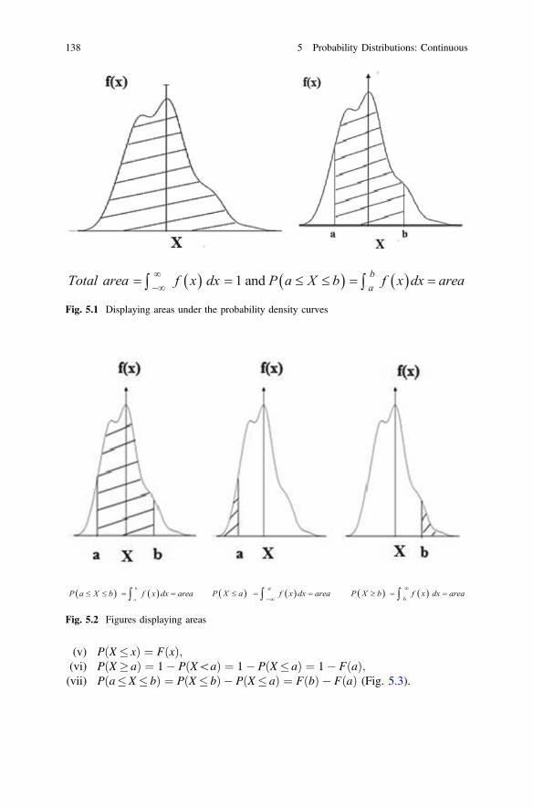
(v) P X � xð Þ ¼ FðxÞ;(vi) P X � að Þ ¼ 1� P X\að Þ ¼ 1� P X� að Þ ¼ 1� FðaÞ;(vii) P a�X� bð Þ ¼ P X � bð Þ � P X� að Þ ¼ FðbÞ � FðaÞ (Fig. 5.3).
Fig. 5.1 Displaying areas under the probability density curves
Fig. 5.2 Figures displaying areas
138 5 Probability Distributions: Continuous

5.3 The Normal Distribution
The normal distribution is one of the most important continuous probability densityfunctions in statistics. It will be seen in the next chapters that the role of the normaldensity function is manyfold. Many measurable characteristics are normally orapproximately normally distributed. The probability density function of the normaldistribution is given by
f x; l; r2� � ¼ 1
rffiffiffiffiffiffi2p
p e�12
x�lrð Þ2 ; �1\x\1;
where (e = 2.71828) and (p = 3.14159).The parameters of the distribution are the mean l and the variance r2. The
continuous random variable, X, which has a normal distribution possessing severalimportant characteristics such as
Fig. 5.3 Figures displaying probabilities greater than or equal to a and between a and b
5.3 The Normal Distribution 139

(i) �1\X\1;(ii) The area under the curve is 1 and it can be shown that
Z1�1
f x; l; r2� �
dx ¼Z1�1
1
rffiffiffiffiffiffi2p
p e�12
x�lrð Þ2dx ¼ 1:
(iii) The density function of X, f(x), is a bell-shaped curve (Fig. 5.4).
The highest point of the curve of f(x) is at the mean l. Hence, themode = mean = l.The curve of f(x) is symmetric about the mean l.In other words, mean = mode = median.The normal distribution depends on two parameters
mean ¼ l and standard deviation ¼ r:
(vii) If the random variable, X, is normally distributed with mean l and standarddeviation r (variance r2), we write X * N l; r2ð Þ.
(viii) The location of the normal distribution depends on l. The scale of thenormal distribution depends on r and if the values of these parameters areknown then the normal distribution is fully specified (Fig. 5.5).
Fig. 5.4 Figure displaying a normal distribution with mean l and variance r2
140 5 Probability Distributions: Continuous

5.4 The Standard Normal Distribution
The normal distribution with mean l ¼ 0 and variance r2 ¼ 1 is called the standardnormal distribution and is denoted by Normal (0,1) or N(0,1). The standard normalrandom variable is denoted by Z, and we write
Z�N 0; 1ð Þ:
It can be shown that if X * Normal l; r2ð Þ, then Z ¼ X�lr * Normal (0,1). The
mean and variance of the standard normal variate, Z, can be shown as follows:
EðZÞ ¼ EX � lr
� �¼ EðXÞ � l
r¼ EðXÞ � l
r¼ l� l
r¼ 0:
It may be noted here that l and r2 are constants and we know that expectedvalues on any constant remain same implying that EðlÞ ¼ l and E 1
r
� � ¼ 1r.
Similarly, variance of Z is
Fig. 5.5 Comparison of normal distributions with X1 �Nðl1;r21Þ and X2 �Nðl2;r22Þ
5.4 The Standard Normal Distribution 141

VarðZÞ ¼ VarX � lr
� �¼ VarðXÞ
r2¼ r2
r2¼ 1:
In this case, as is shown in Chap. 2 that variance is independent of shift in originðlÞ but depends on the change in scale ðrÞ then VarðaXÞ ¼ a2VarðXÞ where a ¼ 1
r
and VarðXÞ ¼ r2.The probability density function (pdf) of Z * N(0,1) is given by (Fig. 5.6)
f ðzÞ ¼ Nðz; 0; 1Þ ¼ 1ffiffiffiffiffiffi2p
p e�12z
2
The standard normal distribution, N(0,1), is very useful and plays a veryimportant role in statistics because area under any normal curve can be calculatedfrom the probabilities of the standard normal distribution due to the fact that boththe mean and variance of the standard normal distribution are known hence thedistribution is fully specified. The following figures indicate the area under speci-fied range of the standard normal variate, Z (Fig. 5.7).
Calculating Probabilities of Normal (0,1)We need to know various probability calculations using the standard normal distri-bution. The value for area under a specified value represents the corresponding prob-ability. Suppose that Z * N (0,1). For the standard normal distribution Z * N(0, 1),there is a special table used to calculate probabilities of the form
P Z � zð Þ:
(i) P Z � að Þ where z = a can be found from the table for Z. The probability ofless than or equal to z = a is given. Sometimes probabilities greater than anyvalue z = a or probabilities in tail areas of a standard normal distribution aregiven too.
Fig. 5.6 Figure displaying astandard normal distribution
142 5 Probability Distributions: Continuous

(ii) PðZ[ bÞ ¼ 1� PðZ� bÞ where PðZ� bÞ can be obtained from the standardnormal table for any specified value of z = b.
(iii) P a� Z� bð Þ ¼ P Z � bð Þ � P z� að Þ where PðZ� bÞ is obtained forz = b and similarly PðZ� aÞ for z = a is also from the table.
Fig. 5.7 Areas under standard normal distribution curve
5.4 The Standard Normal Distribution 143

(iv) If PðZ � aÞ where a\0 then it can be obtained from the table wherePðZ � aÞ is shown for a� 0. In case of a positive value PðZ� aÞ can befound directly from the table as:
20.0 10.0 00.0 z 90.0 ...
0005.0 10.0 ... ... 9535.0
.... ... ... ... ... ...
8999.0 6.3 .. 9999.0 ... ... ...
Example 5.1 If z = 0.94 then find the probability for PðZ� 0:94Þ. Using therelationship in (ii), we obtain
P Z � 0:94ð Þ ¼ 1� P Z� 0:94ð Þ¼ 1� 0:8264
¼ 0:1736
Suppose that Z * N(0,1) then using (i), we can calculate the probability ofZ less than or equal to z = 1.72 as shown below
P Z� 1:72ð Þ ¼ 0:9573
144 5 Probability Distributions: Continuous

(3) If Z * N(0, 1) then the area under z = −1.65 and z = 1.48 can be calculatedusing the standard normal table as follows
Pð�1:65� Z � 1:48Þ ¼ PðZ� 1:48Þ�
PðZ� � 1:65Þ ¼ 0:9306� 0:0548
¼ 0:8758
(4) P Z � 0ð Þ ¼ P Z� 0ð Þ ¼ 0:5(5) To find the value of Z, if area under that value is given, let us define
P Z � zað Þ ¼ a where a is given and we want to find the value of za. As thenormal curve is symmetric about zero, it can also be shown that P Z� z1�að Þ ¼1� a implies that za ¼ �z1�a because P Z� z1�að Þ ¼ 1� P Z � z1�að Þ ¼1� ð1� aÞ ¼ a.
From the above relationship, it is seen that PðZ � z1�aÞ ¼ a. From table, we canwe can find this using the relationship
za ¼ �z1�a:
5.4 The Standard Normal Distribution 145

Some examples are displayed in the following figures:
Example 5.2 Since the pdf of Z * N(0, 1) is symmetric about 0, we have
z1�a ¼ �za; andza ¼ �z1�a:
For example, Z0:48 ¼ �Z1�0:48 ¼ �Z0:52Z0:73 ¼ �Z1�0:73 ¼ �Z0:27:
Suppose that Z * N(0, 1).If P Z � zað Þ ¼ 0:9306Then za ¼ 1:48
z0:0694 ¼ z1�0:9306 ¼ �z0:9306 ¼ �1:48
146 5 Probability Distributions: Continuous

PðZ� zaÞ ¼ 0:9306; PðZ� Z0:9306Þ ¼ 0:9306;za ¼ z0:9306; za ¼ z0:9306 ¼ 1:48;PðZ� z1�aÞ ¼ PðZ � � zaÞPðZ� z1�0:9306Þ ¼ PðZ � � z0:9306Þz0:0694 ¼ z1�0:9306 ¼ �z0:9306 ¼ �1:48:
Example 5.3 Suppose that Z * N(0, 1). Find the value of k such that
PðZ � kÞ ¼ 0:0465:
Solution
k ¼ �1:68; k ¼ Z0:0465 ¼ �1:68
Using the relationship za ¼ �z1�a we find that
z0:0465 ¼ z1�0:9535 ¼ �z0:9535 ¼ �1:68:
5.4 The Standard Normal Distribution 147
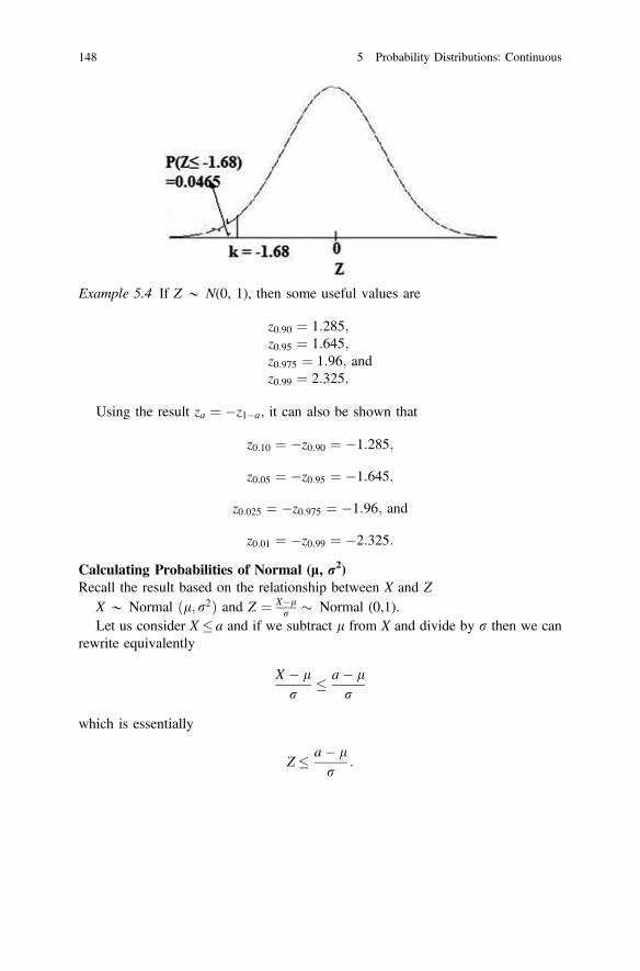
Example 5.4 If Z * N(0, 1), then some useful values are
z0:90 ¼ 1:285;z0:95 ¼ 1:645;z0:975 ¼ 1:96; andz0:99 ¼ 2:325:
Using the result za ¼ �z1�a, it can also be shown that
z0:10 ¼ �z0:90 ¼ �1:285;
z0:05 ¼ �z0:95 ¼ �1:645;
z0:025 ¼ �z0:975 ¼ �1:96; and
z0:01 ¼ �z0:99 ¼ �2:325:
Calculating Probabilities of Normal (l, r2)Recall the result based on the relationship between X and Z
X * Normal l; r2ð Þ and Z ¼ X�lr � Normal (0,1).
Let us consider X � a and if we subtract l from X and divide by r then we canrewrite equivalently
X � lr
� a� lr
which is essentially
Z� a� lr
:
148 5 Probability Distributions: Continuous

Similarly, we can also show the following relationships:
1. P X � að Þ ¼ P Z� a�lr
� �2. P X � að Þ ¼ 1� P X� að Þ ¼ 1� P Z� a�l
r
� �3. P a�X� bð Þ ¼ P X� bð Þ � P X � að Þ ¼ P Z� b� l
r
� �� P Z � a� l
r
� �
ApplicationsFollowing examples show some applications of the normal distribution.
Example 5.5 Let us consider weight of women in reproductive age follows anormal distribution with mean 49 kg and variance 25 kg2
(a) Find the probability that a randomly chosen woman in her reproductive age hasweight less than 45 kg.
(b) What is the percentage of women having weight less than 45 kg?(c) In a population of 20,000 women of reproductive age, how many would you
expect to have weight less than 45 kg?
Solution Here the random variable, X = weight of women in reproductive age,population mean = 49 kg, population variance= r2 = 25 kg2, population standarddeviation = r = 5 kg. Hence, X * Normal (49,25).
(a) The probability that a randomly chosen woman in reproductive age has weightless than 45 kg is P X\45ð Þ:
P X � 45ð Þ ¼ P Z� 45� lr
� �
¼ P Z� 45� 495
� �¼ P Z � � 0:8ð Þ¼ 0:2119:
(b) The percentage of women of reproductive age who have weight less than 45 kgis P X � 45ð Þ � 100% = 0.2119 � 100% = 21.19%
(c) In a population of 20,000 women of reproductive age, we would expect that thenumber of women with weight less than 45 kg is P X� 45ð Þ � 20,000 =0.2119 � 20,000 = 4238.
Example 5.6 Let us consider that the birth weight of girls in rural community ofBangladesh is 2.59 kg ðlÞ and the standard deviation is 0.43 kg ðrÞ.(a) Find the probability that a randomly chosen girl has a birth weight between 3.0
and 4.0 kg.(b) What is the percentage of girls who have a birth weight between 3.0 and
4.0 kg?
5.4 The Standard Normal Distribution 149

(c) In a population of 100,000 girls, how many would you expect to have birthweight between 3.0 and 4.0 kg?
Solution The random variable is X = birth weight of a girl in rural community inBangladesh, the population mean, l = 2.59 kg, the population standard deviation,r = 0.43 kg, the population variance, r2 = (0.43 kg)2 = 0.1849 kg2, and it isassumed that X is normally distributed then X * N (2.59,0.1849).
(a) The probability that a randomly chosen girl has a birth weight between 3.0 and4.0 kg is P 3:0\X\4:0ð Þ.
P 3:0\X\4:0ð Þ ¼ P X\4:0ð Þ � P X � 3:0ð Þ
¼ P Z\4:0� l
r
� �� P Z� 3:0� l
r
� �
¼ P Z\4:0� 2:59
0:43
� �� P Z� 3:0� 2:59
0:43
� �¼ P Z\3:27ð Þ � PðZ � 0:95Þ¼ 0:99946� 0:82894 ¼ 0:17052:
(b) The percentage of girls who have a birth weight between 3.0 and 4.0 kg is
P 3:0\X\4:0ð Þ � 100% ¼ 0:17052� 100% ¼ 17:05%
(c) In a population of 100,000 Bangladeshi girls community, we would expect thatthe number of babies with birth weight between 3.0 and 4.0 kg to be
P 3:0\X\4:0ð Þ � 100,000 ¼ 0:17052� 100,000 ¼ 17,052 girls:
5.5 Normal Approximation for Binomial Distribution
Suppose that the random variable, X, has a binomial distribution with parameters, nand p, that is X * Binomial (n,p). If the number of trial is large (n ! ∞), and theprobability of success is close to half (p ! 0.5), then the binomial distribution,binomial (n,p), can be approximated by Normal distribution N(l, r2),where l ¼ npand r2 ¼ npð1� pÞ. That is, for large n, we have
Binomialðn; pÞ � Nðnp; npð1� pÞÞ:
150 5 Probability Distributions: Continuous

Then it can be shown that
X � npffiffiffiffiffiffiffiffiffiffiffiffiffiffiffiffiffiffiffiffinpð1� pÞp � Nð0; 1Þ:
As X is a discrete variable and it has limiting distribution that is N(0,1), we needa continuity correction to obtain probability for an interval
PðX ¼ xÞ ¼ Pðx� 0:5\X\xþ 0:5Þ� P x�0:5�npffiffiffiffiffiffiffiffiffiffiffiffi
npð1�pÞp \Z\ xþ 0:5�npffiffiffiffiffiffiffiffiffiffiffiffi
npð1�pÞp
:
Similarly, we can find the following probabilities using the limiting distribution:
PðX� xÞ ¼ PðX\xþ 0:5Þ � P Z\xþ 0:5� npffiffiffiffiffiffiffiffiffiffiffiffiffiffiffiffiffiffiffiffi
npð1� pÞp" #
;
PðX � xÞ ¼ PðX[ x� 0:5Þ � P Z[x� 0:5� npffiffiffiffiffiffiffiffiffiffiffiffiffiffiffiffiffiffiffiffi
npð1� pÞp" #
; and
Pðx1 �X � x2Þ
¼ Pðx1 � 0:5\X\x2 þ 0:5Þ � Px1 � 0:5� npffiffiffiffiffiffiffiffiffiffiffiffiffiffiffiffiffiffiffiffi
npð1� pÞp \Z\x2 þ 0:5� npffiffiffiffiffiffiffiffiffiffiffiffiffiffiffiffiffiffiffiffi
npð1� pÞp" #
:
The following figures illustrate the idea of the continuity correction for the casePðX ¼ xÞ and for the case PðX � xÞ (Fig. 5.8).
Fig. 5.8 Binomialprobability using continuitycorrection for normalapproximation
5.5 Normal Approximation for Binomial Distribution 151

Example 5.7 Suppose that the random variable X has a binomial distribution withparameters n = 100 and p = 0.5, i.e., X * Binomial(100,0.5). Find PðX� 45Þusing an exact method and an approximated method.
Solution
(a) Calculating the exact probability using the fact that X * Binomial(100,0.5):
PðX � 45Þ ¼ P45x¼0
100x
� �� 0:5x � 0:5100�x ¼ 0:1841:
(b) Calculating the approximated probability using normal approximation
We notice that n = 100 (n is large) and p = 0.5. The mean and the variance ofthe distribution are, respectively,
l ¼ np ¼ 100� 0:5 ¼ 50
r2 ¼ npð1� pÞ ¼ 100� 0:5� 0:5 ¼ 25:
Therefore, we can approximate the distribution of X by the normal distributionwith mean l = 50 and variance r2 ¼ 25, as follows:
PðX� 45Þ ¼ PðX\45þ 0:5Þ ¼ PðX\45:5Þ � P Z\45:5� 50ffiffiffiffiffi
25p
� �¼ 0:1841:
5.6 Summary
Two of the most essential continuous distributions, the normal probability distri-bution and the standard normal probability distribution, are discussed in this chapterwith specific focus to the need of users who want to use these distributions in theirapplications. In this chapter, examples are displayed in a way that the users will beable to learn the applications of these distributions without ambiguity. The generalrules of a continuous distribution are illustrated and the relationship betweenprobability in an interval and cumulative probability are shown. The computationalprocedures of probabilities are illustrated with many examples and figures using thestandard normal probability distributions.
Exercises
5:1 Find the following probabilities using the standard normal distribution:
(i) PðZ � 0Þ;(ii) PðZ ¼ 1Þ;(iii) PðZ � 1Þ;(iv) PðZ � � 1Þ;
152 5 Probability Distributions: Continuous

(v) PðZ � 1Þ;(vi) PðZ � � 1Þ;(vii) PðZ � 1:75Þ;(viii) PðZ � � 1:75Þ;(ix) Pð1:68� Z � 2:75Þ;(x) Pð�1� Z � 1Þ; and(xi) Pð�1� Z � 2:45Þ:
5:2 Find the values of the standard normal variate for the following probabilities:
(i) PðZ � zaÞ ¼ 0:975;(ii) PðZ � zaÞ ¼ 0:025;(iii) PðZ � z0:05Þ ¼;(iv) PðZ � zaÞ ¼ 0:01;(v) PðZ � zaÞ ¼ 0:99;(vi) PðZ � zaÞ ¼ 0:35; and(vii) PðZ � zaÞ ¼ 0:65:
5:3 Using the relationship Za ¼ �Z1�a, find the following values of the standardnormal distribution variable:
(i) z0:2;(ii) z0:7;(iii) z0:01; and(iv) z0:9:
5:4 For a normally distributed variable, X, where X �Nð25; 9Þ, find the followingprobabilities:
(i) PðX � 25Þ;(ii) PðX � 10Þ; and(iii) Pð15�X� 40Þ:
5:5 Suppose that the mean duration of suffering from a viral infection is dis-tributed normally with mean 10 days and standard deviation 5 days.
(i) Find the probability that a randomly selected subject will suffer for lessthan 7 days.
(ii) Find the probability that a randomly selected subject will suffer from theviral infection for more than 5 days.
(iii) Find the probability that the subject will suffer from the viral infectionfor 8 to 12 days.
(iv) Find the number of days above which 70% of the subjects will sufferfrom viral infection.
5.6 Summary 153

5:6 Suppose that the money spent for medical purpose in among the elderly in acommunity is $50 per month with a standard deviation $9.
(i) Find the amount of money or less spent by an elderly person in a monthsuch that the probability is 0.75.
(ii) Find the probability that an elderly person will spend less than $30.(iii) Find the amount of money or more spent by an elderly subject with
probability 0.9.
5:7 In a study, it is found that the proportion of underweight children under5 years in a community is 0.41. Let the sample size n = 200 and the randomvariable X denotes the number of underweight children.
(i) Find the probability that the number of underweight children is less than40.
(ii) Find the probability that the number of underweight children is greaterthan 90.
(iii) Find the probability that the number of children lies between 50 and 80.
154 5 Probability Distributions: Continuous
Chapter 6Sampling Distribution
6.1 Sampling Distribution
The probability distribution of a statistic is called the sampling distribution of thatstatistic. The sampling distribution of the statistic is used to make statistical in-ference about the unknown parameter. There may be question regarding probabilitydistribution of a statistic when the probability distribution of a variable is known. Itinvolves the role of a random sample in statistics. Let us consider a variable, X, andthe population of X is comprised of N elements denoted by ðX1; . . .;XNÞ whichmeans that whenever we draw a sample of size, n, the values in the sample must beselected from these elements in the population. Before a sample is drawn, we do nothave any idea which values from the population are being selected although it isknown that n values in the sample must be from N values in the population. In thatcase for each value of the sample, a random variable can be defined, which aredenoted by ðX1; . . .;XnÞ. The realization of random sample can be represented asX1 ¼ x1; . . .;Xn ¼ xn where x1; . . .; xnð Þ. A random sample implies that each randomvariable in a random sample can take any of the N values from the population. Inother words, n random variables in the random sample may take N � . . .� N ¼ Nn
possible samples with replacement. Here, the term with replacement indicates that ifone value from the population is already selected can be considered for beingselected again in subsequent draws in the same sample. That is the populationvalues can be selected multiple times in a sample. To avoid this repetition in thesame sample, we may use the other approach named as sampling withoutreplacement. Sampling without replacement ensures that if one value is drawnalready from the population in a sample, it will be dropped from the next selection.In that case, the number of possible samples is N � ðN � 1Þ � . . .� ðN � nþ 1Þwhere there is no replacement in a single sample and considering the order ofselection. However, due to change in the order of selection in the sample whichoccurs in n! ways, there are n! samples with same elements if the order is consideredin samples. Hence, to select samples without repetition within the sample (without
© Springer Nature Singapore Pte Ltd. 2018M. A. Islam and A. Al-Shiha, Foundations of Biostatistics,https://doi.org/10.1007/978-981-10-8627-4_6
155

replacement) or between samples (disregarding order), we have N � ðN � 1Þ �
. . .� ðN � nþ 1Þ=n! ¼ N
n
!samples without replacement disregarding the order
of selection in samples. This has a very useful interpretation with deep-rootedimplications in statistics. Let us illustrate with a small population size in the fol-lowing example.
Example 6.1 Let us consider a population with four elements represented byX1 ¼ 1;X2 ¼ 3;X3 ¼ 2; and X4 ¼ 4. The population size is N = 4. We want todraw a sample of size n = 2. Let us define the random sample as X1;X2ð Þ. Then wecan select the samples by either with replacement or without replacement.
With replacement: The number of samples with replacement is 24 ¼ 16. Thesamples are: (1, 1), (1, 3), (1, 2), (1, 4), (3, 1), (3, 3), (3, 2), (3, 4), (2, 1), (2, 3),(2, 2), (2, 4), (4, 1), (4, 3), (4, 2), (4, 4).
Without replacement: The number of samples without replacement in eachsample is 4� 3 ¼ 12 and the samples are (1, 3), (1, 2), (1, 4), (3, 1), (3, 2), (3, 4),(2, 1), (2, 3), (2, 4), (4, 1), (4, 3), (4, 2). It is clearly seen from these possiblesamples that each sample is repeated 2! ¼ 2� 1 times if we disregard the order ofselection such as (1, 3) and (3, 1). Hence, the number of samples withoutreplacement within each sample (without replacement) and between samples (dis-
regarding order) is4
2
!¼ 6. If we consider without replacement and disregard
order then the samples are: (1, 3), (1, 2), (1, 4), (3, 2), (3, 4), and (2, 4).We have discussed about the random sample with or without replacement above.
The important point here is that we select only one sample out of all the possiblesamples using with or without replacement. Let us consider a hypothetical situationwhere all the possible samples could be drawn of same sample size, n. In that situation,we could find the value of statistic for all the possible samples. As an example, let usconsider about the statistic, sample mean. If there are Nn possible samples withreplacement then the number of values of statistic, mean, will be Nn too. Similarly,
disregarding order the number of samples without replacement isN
n
!. We can find
the frequency distribution and probability distribution of the mean based on thesevalues. This probability distribution is known as the sampling distribution. In otherwords, probability distribution of a statistic is known as the sampling distribution.
6.2 Sampling Distribution of the Sample Mean
The sampling distribution of the sample mean is widely used in statistics. Supposethat we have a population with mean l and variance r2 and let X1;X2; . . .;Xn be a
156 6 Sampling Distribution

random sample of size n selected randomly from this population. We know that thesample mean is
�X ¼Pn
i¼1 Xi
n:
Example 6.2 Let us consider a population of size N = 5 and a sample of size n = 3.The population elements are X1 ¼ 30;X2 ¼ 25;X3 ¼ 40;X4 ¼ 27; and X5 ¼ 35.The random sample is X1;X2;X3ð Þ. All the possible samples, disregarding order andobtained without replacement randomly, are shown below. The number of samples
using without replacement and disregarding order is5
3
!¼ 10. The population
mean is l ¼P5
iXi
5 ¼ 1575 ¼ 31:40.
The mean of the sample means is Table 6.1
l ¼P10
i�Xi
10¼ 314
10¼ 31:40:
The population mean of the variable X and the population mean of means fromthe random samples of size n are exactly the same. From the above example, weobserve that in both the cases, the mean is 31.40. This can be summarized as
EðXÞ ¼ l;
Eð�XÞ ¼ l:
This is an important property of the sampling distribution of mean.It is observed that the value of the sample mean, X, varies from one random
sample to another. The value of X is random and it depends on the random sample.Hence, the sample mean X is a random variable. The probability distribution of X iscalled the sampling distribution of the sample mean, X.
Table 6.1 Sample means ofall possible samples of size 3from a population of size 5
Sample X1 X2 X3 �X
1 30 25 40 31.67
2 30 25 27 27.33
3 30 25 35 30.00
4 30 40 27 32.33
5 30 40 35 35.00
6 30 27 35 30.67
7 25 40 27 30.67
8 25 27 35 29.00
9 25 40 35 33.33
10 40 27 35 34.00
6.2 Sampling Distribution of the Sample Mean 157

For the sampling distribution of the sample mean, we need to know the form ofthe sampling distribution, the expected value of the mean of the sample mean, �X,and the variance of the sample mean, �X.
6.3 Some Important Characteristics of the SamplingDistribution of X
Mean and Variance of XIf X1;X2; . . .;Xn is a random sample of size n from any distribution with mean l
and variance r2, then:
1. The mean of X is
l�X ¼ l:
2. The variance of X is
r2�X ¼ r2
n:
3. The standard deviation of X is called the standard error of X and is defined by
r�X ¼ffiffiffiffiffiffir2�X
q¼ rffiffiffi
np :
It may be noted here that the square root of the variance of a statistic is termed asstandard error. In this case, the standard error of the sample mean is rffiffi
np .
6.4 Sampling from Normal Population
If X1;X2; . . .;Xn is a random sample of size n from a normal population with meanl and variance r2 that is Normal l; r2ð Þ, then the sample mean has a normaldistribution with mean l and variance r2=n that is
158 6 Sampling Distribution

1. X � Normal l; r2
n
� �.
The sampling distribution of the sample mean, �X, can be shown as
f ð�x; l; r2=nÞ ¼ 1ffiffiffiffiffiffiffiffiffiffiffiffiffiffiffi2pr2=n
p e�n
2r2ð�x�lÞ2 ;�1\�x\1:
This is also a normal distribution with the same expected value as the expectedvalue of X but with a different variance. The expected value of �X is
Eð�XÞ ¼ EX1 þ . . .þXn
n
� �
¼ EðX1Þþ . . .þEðXnÞn
¼ lþ . . .þ ln
¼ l:
We know that the random samples can take values randomly from the populationwith probability density function X �Nðl; r2Þ. Hence, EðX1Þ ¼ . . . ¼ EðXnÞ ¼ l.
Similarly, the variance of the sample mean, if X1; . . .;Xn are independent, is
Varð�XÞ ¼ VarX1 þ . . .þXn
n
� �
¼ VarðX1Þþ . . .þVarðXnÞn2
¼ r2 þ . . .þ r2
n2
¼ nr2
n2
¼ r2
n:
For variance also, the random variable in a random sample satisfies theassumption that X �Nðl; r2Þ where population mean and population varianceremain same for all the random variables in a random sample. Hence, it can beshown that VarðX1Þ ¼ . . . ¼ VarðXnÞ ¼ r2.
2. Z ¼ �X�lr=ffiffin
p �Normal ð0; 1Þ:We use this result when sampling from normal distribution with known variance
r2. As we have shown that if X �Nðl; r2Þ then �X�Nðl; r2=nÞ implying that thesampling distribution of the sample mean follows the normal distribution as well.Hence, the standardized normal variate can be obtained for the sample mean as arandom variable which is
6.4 Sampling from Normal Population 159

Z ¼�X � lr=
ffiffiffin
p ;
where Z�Nð0; 1Þ.
6.4.1 Central Limit Theorem: Sampling from Non-normalPopulation
Let X1;X2; . . .;Xn be a random sample of size n from non-normal population withmean l and variance r2. If the sample size n is large or if n ! 1 then the samplemean has approximately a normal distribution with mean l and variance r2=n thatis
(i) X � Normal l; r2
n
� �;
(ii) Z ¼ �X�lr=ffiffin
p � Nð0; 1Þ Normal ð0; 1Þ:
Note: “�” means “approximately distributed”.We can use this result when sampling from non-normal distribution with known
variance r2 and with large sample size too.
6.4.2 If r2 is Unknown and Sample is Drawn from NormalPopulation
If X1;X2; . . .;Xn is a random sample of size n from a normal distribution with meanl and unknown variance r2 that is Normal l; r2ð Þ, then the statistic
T ¼�X � lS=
ffiffiffin
p
has a t-distribution with ðn� 1Þ degrees of freedom, where S is the sample standarddeviation given by
S ¼ffiffiffiffiffiS2
p¼
ffiffiffiffiffiffiffiffiffiffiffiffiffiffiffiffiffiffiffiffiffiffiffiffiffiffiffiffiffiffiffiPni¼1 Xi � X� �2n� 1
s:
160 6 Sampling Distribution

We write
T ¼�X � lS=
ffiffiffin
p � tðn� 1Þ;
where the sampling distribution of T is known as t-distribution with degrees offreedom = df = m = n − 1.
6.5 The T-Distribution
The Student’s t-distribution is a distribution of a continuous random variable similarto Z defined earlier. The difference between t and Z lies in the fact that althoughboth assume the random sample X1, X2, …, Xn is a random sample of size n from anormal distribution with mean l and variance r2, i.e., N(l, r2), r2 is assumed to beknown for defining Z but it is not known for t and hence needs to be estimated. Wedefined Z as
Z ¼�X � lr=
ffiffiffin
p �Nð0; 1Þ
which is theoretically correct if r2 is known. If r2 is unknown, we replace thepopulation variance r2 with the sample variance
S2 ¼Pn
i¼1 Xi � X� �2n� 1
to define the following statistic known as T or Student’s T
T ¼�X � lS=
ffiffiffin
p :
Then we can define the statistic T more precisely as follows. If (X1, X2, …, Xn) isa random sample of size n from a normal distribution and the random variables areindependent with mean l and variance r2, i.e., N(l, r2), then the statistic
T ¼�X � lS=
ffiffiffin
p
has a t-distribution with (n − 1) degrees of freedom and we write T � tðmÞ orT � tðn�1Þ. The t-distribution with m degrees of freedom is
6.4 Sampling from Normal Population 161

f ðt; mÞ ¼ Þðmþ 1Þ=2Þm=2 ffiffiffiffiffi
pmp 1þ t2
m
�ðmþ 1Þ2
; �1\t\1:
The mean and variance of T are
EðTÞ ¼ 0;
VarðTÞ ¼ mm� 2
; m[ 2:
The t-distribution is a continuous distribution, the value of random variableT ranges from −∞ to +∞ (that is, −∞ < t < ∞), the mean of T is 0, variance ism=ðm� 2Þ, and the shape of t-distribution is similar to the shape of the standardnormal distribution. It may also be noted that t-distribution ! standard normaldistribution as n ! ∞.
The following figure displays the t-distribution curves for different degrees offreedom. It shows that as the degrees of freedom increases, the t-distribution curvetends to standard normal distribution (Figs. 6.1 and 6.2).
Fig. 6.1 Comparison between normal and t-distributions
162 6 Sampling Distribution

Area under the t-distribution curves is shown for P(T < ta) and P(T < t1−a) in thefigures displayed below. The mean of T is zero and the curve is symmetric thatresults in ta = −t1−a or t1−a = −ta.
It may be noted here that
(i) ta = the t-value under which we find an area equal to a = the t-value thatcovers an area of a to the left.
(ii) The value ta satisfies: P(T < ta)= a.(iii) Since the curve of the pdf of T * t(m) is symmetric about 0, we have
t1�a ¼ �ta;
for example t0.35 = −t1−0.35 = −t0.65, t0.86 = −t1−0.86 = −t0.14.
(iv) In a table for t-distribution, the values of ta are given for degrees of freedom. Inother words, the value of t depends on degrees of freedom which implies that ifthe degree of freedom is specified then the area under a certain value ofT = t can be determined.
Example 6.3 Find the t-value with m = 14 that shows an area of
(a) 0.95 to the left,(b) 0.95 to the right.
SolutionHere it is given that m = 14 which is and T * t14 (Fig. 6.3).
Fig. 6.2 Areas of t-distribution to the left and right tails
6.5 The T-Distribution 163

(a) The t-value that determines an area of 0.95 to the left is
t0:95 ¼ 1:761:
(b) The t-value that leaves an area of 0.95 to the right is (Fig. 6.4)
t0:05 ¼ �t1�0:05 ¼ �t0:95 ¼ �1:761
Note: Some t-tables contain values of a that are greater than or equal to 0.90. Whenwe search for small values of a in these tables, we may use the fact that
Fig. 6.3 Area of t to the left with 14 degrees of freedom
Fig. 6.4 Area of t to the right with 14 degrees of freedom
164 6 Sampling Distribution

t1�a ¼ �ta
Example 6.4 For m = 10 degrees of freedom, find t0.93 and t0.07.
Solution
t0.93= (1.372 + 1.812)/2 = 1.592 (from the table)t0.07 = −t1−0.07 = −t0.93 = −1.592 (using the rule: t1−a = −ta) (Fig. 6.5)
Applications
Example 6.5 Let us consider that the temperature of patients with acute nephritis ofrenal pelvis origin may be greater than the individuals without having this diseaserise and let the temperature of patients is normally distributed with the populationmean 38.7 °C and the population standard deviation 1.82 Â °C. Find the proba-bility that a random sample of 40 patients will have average temperature less than38 °C.
Solution
X = the temperature of patient with acute nephritis of renal pelvis origin,l = 38.7 °C,r = 1.82 °C,r2 = 3.31 °C2,X�Nð38:7; 3:31Þ,Sample size, n = 40.
It has been shown earlier that the sampling distribution �X is �X�N l; r2=nð Þ. Thesample mean obtained from the sample of size 40 is �x ¼ 37 and the population
Fig. 6.5 t0.93 for v = 10
6.5 The T-Distribution 165

variance is assumed to be known as r2 = 3.31 °C2. Hence, the standard error of the
mean is r�X ¼ffiffiffiffir2n
q¼
ffiffiffiffiffiffi3:3140
q¼ ffiffiffiffiffiffiffiffiffiffiffiffiffiffiffiffi
0:08275p ¼ 0:2877.
Using the central limit theorem, �X has a normal distribution with mean l�X ¼38:7 and variance r2�X ¼ 0:2877 that is
�X�N l;r2
n
¼ N 38:7; 0:2877ð Þ
Z ¼�X � lr=
ffiffiffin
p ¼�X � 38:70:2877
�N 0; 1ð Þ
The probability that a random sample of 40 patients with acute nephritis of renalpelvis origin will have an average temperature of less than 38 °C is
Pð�X\38Þ ¼ P�X � lr=
ffiffiffin
p \38� l
1:82=ffiffiffiffiffi40
p
¼ P�X � 38:7
1:82=ffiffiffiffiffi40
p \38� 38:70:2877
¼ P Z\38� 38:70:2877
¼ P Z\� 2:43ð Þ¼ 0:007549:
Example 6.6 If the mean and standard deviation of height of women in theirreproductive age is 152 cm and standard deviation is 5 cm then find the probabilitythat a random sample of size 50 women will yield a mean height between 150 and154 cm.
Solution
X = the height of a woman in her reproductive period,l = 152 cm,r = 5 cm,r2 = 25 cm2,X�Nð152; 25Þ,Sample size, n = 50.
It has been shown earlier that the sampling distribution �X is �X�N l; r2=nð Þ. Thestandard error of the mean is r�X ¼
ffiffiffiffir2n
q¼
ffiffiffiffi2550
q¼ ffiffiffiffiffiffiffiffiffi
0:50p ¼ 0:7071.
Using the central limit theorem, �X has a normal distribution with mean l�X ¼152 cm and variance r2�X ¼ 0:50 cm2 that is
166 6 Sampling Distribution

�X�N l;r2
n
¼ N 152; 0:50ð Þ
and it can be shown that
Z ¼�X � lr=
ffiffiffin
p ¼�X � 1520:7071
�N 0; 1ð Þ:
The probability that the random sample of 50 women will yield average heightin-between 150 and 154 cm is
Pð150\�X\154Þ ¼ P150� l
5=ffiffiffiffiffi50
p \�X � lr=
ffiffiffin
p \154� l
5=ffiffiffiffiffi50
p !
¼ P150� 152
5=ffiffiffiffiffi50
p \Z\154� 152
5=ffiffiffiffiffi50
p !
¼ P �1:4142\Z\1:4142ð Þ¼ P Z\1:4142ð Þ � P Z\� 1:4142ð Þ¼ 0:9213� 0:0787 ¼ 0:8426
Example 6.7 t-distribution for single sampleLet us consider that in a rural population, the mean weight of women in their
reproductive ages is 52 kg. The population variance is not known. Using the datafrom a sample of size n = 24 from a normally distributed population, the samplevariance is s2 = 90.0217. Find the probability that a randomly selected woman ofchildbearing age has weight less than 49 kg. Also, find the probability that arandomly selected woman of childbearing age has weight in between 49 and 53 kg.
SolutionX = the weight of women in their childbearing age in a rural community,l = 52 kg
S ¼ffiffiffiffiffiffiffiffiffiffiffiffiffiffiffiffi90:0217
p¼ 9:4880 kg;
X�Nðl; r2Þ;
sample size, n = 24.It is shown earlier that if r2 is unknown, then we use the sample variance and
replace the population variance r2 with
S2 ¼Pn
i¼1 Xi � X� �2n� 1
:
6.5 The T-Distribution 167

The Student’s T is defined as
T ¼�X � lS=
ffiffiffin
p ;
where T � tðmÞ or T � tðn�1Þ. The standard error of the mean for unknown variance isffiffiffiffiS2n
q¼
ffiffiffiffiffiffiffiffiffiffiffi90:0217
24
q¼ ffiffiffiffiffiffiffiffiffiffiffiffiffiffi
3:7509p ¼ 1:9367.
Now using the above results, we obtain
T ¼�X � lS=
ffiffiffin
p ¼�X � 521:9367
which is tð23Þ.The probability that a random sample of weights of 24 women in their child-
bearing period is less than 49 kg is
Pð�X\49Þ ¼ P�X � lS=
ffiffiffin
p \49� l
9; 4880=ffiffiffiffiffi24
p !
¼ P�X � lS=
ffiffiffin
p \49� 521:9367
¼ P T\49� 521:9367
¼ P T\� 1:5490ð Þ ¼ 0:0675:
Now if we want to find the probability that a randomly selected woman will haveweight in between 49 and 53 kg then
Pð49\�X\53Þ ¼ P49� l
9; 4880=ffiffiffiffiffi24
p \�X � lS=
ffiffiffin
p \53� l
9; 4880=ffiffiffiffiffi24
p !
¼ P49� 521:9367
\�X � lS=
ffiffiffin
p \53� 521:9367
¼ P49� 521:9367
\T\53� 521:9367
¼ P �1:5490\T\0:5163ð Þ:
From the t-table, this probability can be obtained from the following:
P �1:5490\T\0:5163ð Þ ¼ P T\0:5163ð Þ � P T\� 1:5490ð Þ¼ 0:6947� 0:0675 ¼ 0:6272:
168 6 Sampling Distribution
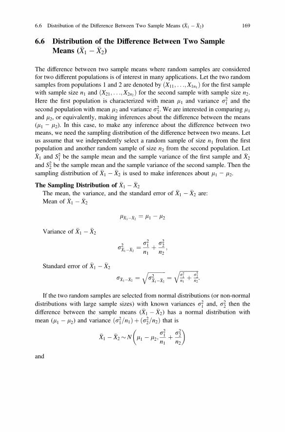
6.6 Distribution of the Difference Between Two SampleMeans (�X1 � �X2)
The difference between two sample means where random samples are consideredfor two different populations is of interest in many applications. Let the two randomsamples from populations 1 and 2 are denoted by X11; . . .;X1n1ð Þ for the first samplewith sample size n1 and X21; . . .;X2n2ð Þ for the second sample with sample size n2.Here the first population is characterized with mean l1 and variance r21 and thesecond population with mean l2 and variance r22. We are interested in comparing l1and l2, or equivalently, making inferences about the difference between the means(l1 − l2). In this case, to make any inference about the difference between twomeans, we need the sampling distribution of the difference between two means. Letus assume that we independently select a random sample of size n1 from the firstpopulation and another random sample of size n2 from the second population. Let�X1 and S21 be the sample mean and the sample variance of the first sample and �X2
and S22 be the sample mean and the sample variance of the second sample. Then thesampling distribution of �X1 � �X2 is used to make inferences about l1 − l2.
The Sampling Distribution of �X1 � �X2
The mean, the variance, and the standard error of �X1 � �X2 are:Mean of �X1 � �X2
l�X1��X2¼ l1 � l2
Variance of �X1 � �X2
r2�X1��X2¼ r21
n1þ r22
n2;
Standard error of �X1 � �X2
r�X1��X2¼
ffiffiffiffiffiffiffiffiffiffiffiffiffir2�X1��X2
q¼
ffiffiffiffiffiffiffiffiffiffiffiffiffiffir21n1
þ r22n2
q.
If the two random samples are selected from normal distributions (or non-normaldistributions with large sample sizes) with known variances r21 and, r22 then thedifference between the sample means (�X1 � �X2) has a normal distribution withmean (l1 � l2) and variance ðr21=n1Þþ ðr22=n2Þ that is
�X1 � �X2 �N l1 � l2;r21n1
þ r22n2
and
6.6 Distribution of the Difference Between Two Sample Means (�X1 � �X2) 169

Z ¼ ð�X1 � �X2Þ � ðl1 � l2Þffiffiffiffiffiffiffiffiffiffiffiffiffiffir21n1
þ r22n2
q �N 0; 1ð Þ:
In the above mentioned sampling distribution for the difference between twomeans, the population variances are assumed to be known. If that assumption doesnot hold true then we need to replace the population variance by the samplevariance as shown before in case of single sample. Let us consider that the dif-ference between the sample means is
�X1 � �X2 �N l1 � l2;r21n1
þ r22n2
as before and the sample variances for samples 1 and 2 are
S21 ¼Pn1i¼1
ðX1i � X1Þ2
n1 � 1; and
S22 ¼Pn2i¼1
ðX2i � X2Þ2
n2 � 1:
Then we can define the statistic T as follows:
T ¼ ð�X1 � �X2Þ � ðl1 � l2ÞffiffiffiffiffiffiffiffiffiffiffiffiffiffiS21n1þ S22
n2
q � tðn1 þ n2�2Þ
which is distributed as t with n1 þ n2 � 2ð Þ degrees of freedom. Here, degrees offreedom are reduced by 2 from the total sample size, one from each sample, due tothe following reasons: (i) Initially, we assumed that the random variables in therandom samples from populations 1 and 2 have probability distributionsX1i �Nðl1; r21Þ and X2i �Nðl2; r22Þ respectively; (ii) If r21 and r22 are unknownthen while defining S21 and S22 for the random samples 1 and 2 respectively toreplace the corresponding population variances, we need to assume that populationmeans remain fixed that means the random samples have expected values equal tothe population means that are given by the sample means from the two randomsamples. This restricts the random sample such that ðn1 � 1Þ and ðn2 � 1Þ values ofrandom samples 1 and 2 can be drawn randomly from populations 1 and 2,respectively, without restrictions but to satisfy the condition that the random sampleshave the means equal to the population means, one of the values from each randomsample has to be constrained to make the random sample mean equal to the corre-sponding population. (iii) Hence, one degree of freedom is lost from each sampleresulting in a total degrees of freedom = ðn1 � 1Þþ ðn2 � 1Þ ¼ ðn1 þ n2 � 2Þ.
170 6 Sampling Distribution

Application
Example 6.8 Let us consider birth weights of two groups of babies with means andstandard deviations of 3.3 and 0.6 kg for the first group and 3.1 and 0.5 kg for thesecond group. Find the probability of difference between means of birth weights fromrandom samples of two groups of babies is greater than 0.3 kg. Let the sample size forthe first group is 100 and the second group is 125. Also, find the probability of adifference between mean weights of two groups of babies between 0.1 and 0.3 kg.
SolutionFor the first group:
l1 ¼ 3:3 kg, r1 ¼ 0:6 kg, r21 ¼ 0:36 kg2, n1 ¼ 100.
For the second group:
l2 ¼ 3:1 kg, r2 ¼ 0:5 kg, r22 ¼ 0:25 kg2, n2 ¼ 125.
The mean, the variance, and the standard error of �X1 � �X2 are shown below.Mean of �X1 � �X2 is
l�X1��X2¼ l1 � l2 ¼ 3:3� 3:1 ¼ 0:2:
The variance of �X1 � �X2 is
r2�X1��X2¼ r21
n1þ r22
n2¼ 0:36
100þ 0:25
125¼ 0:0056:
The standard error of �X1 � �X2 is
r�X1��X2¼
ffiffiffiffiffiffiffiffiffiffiffiffiffir2�X1��X2
q¼
ffiffiffiffiffiffiffiffiffiffiffiffiffiffi0:0056
p¼ 0:0748:
The sampling distribution of �X1 � �X2 is
�X1 � �X2 �N 0:2; 0:0056ð Þ:
It can be shown that
Z ¼�X1 � �X2ð Þ � 0:2ffiffiffiffiffiffiffiffiffiffiffiffiffiffi
0:0056p �Nð0; 1Þ:
We can now find the probability of the difference between means of birthweights greater than 0.3 kg from the following steps:
P �X1 � �X2 [ 0:3ð Þ ¼ Pð�X1 � �X2Þ � ðl1 � l2Þffiffiffiffiffiffiffiffiffiffiffiffiffiffi
r21n1
þ r22n2
q [0:3� ðl1 � l2Þffiffiffiffiffiffiffiffiffiffiffiffiffiffi
r21n1
þ r22n2
q0B@
1CA
6.6 Distribution of the Difference Between Two Sample Means (�X1 � �X2) 171
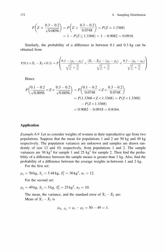
P Z[0:3� 0:2ffiffiffiffiffiffiffiffiffiffiffiffiffiffi0:0056
p
¼ P Z[0:3� 0:20:0748
¼ P Z[ 1:3368ð Þ
¼ 1� P Z� 1:3368ð Þ ¼ 1� 0:9082 ¼ 0:0918:
Similarly, the probability of a difference in between 0.1 and 0.3 kg can beobtained from
Pð0:1\�X1 � �X2\0:3Þ ¼ P0:1� ðl1 � l2Þffiffiffiffiffiffiffiffiffiffiffiffiffiffi
r21n1þ r22
n2
q \ð�X1 � �X2Þ � ðl1 � l2Þffiffiffiffiffiffiffiffiffiffiffiffiffiffi
r21n1þ r22
n2
q \0:3� ðl1 � l2Þffiffiffiffiffiffiffiffiffiffiffiffiffiffi
r21n1þ r22
n2
q0B@
1CA
Hence
P0:1� 0:2ffiffiffiffiffiffiffiffiffiffiffiffiffiffi0:0056
p \Z\0:3� 0:2ffiffiffiffiffiffiffiffiffiffiffiffiffiffi0:0056
p
¼ P0:1� 0:20:0748
\Z\0:3� 0:20:0748
¼ P 1:3368\Z\1:3368ð Þ ¼ P Z\1:3368ð Þ
� P Z\1:3368ð Þ¼ 0:9082� 0:0918 ¼ 0:8164:
Application
Example 6.9 Let us consider weights of women in their reproductive age from twopopulations. Suppose that the mean for populations 1 and 2 are 50 kg and 49 kgrespectively. The population variances are unknown and samples are drawn ran-domly of size 12 and 10, respectively, from populations 1 and 2. The samplevariances are 30 kg2 for sample 1 and 25 kg2 for sample 2. Then find the proba-bility of a difference between the sample means is greater than 3 kg. Also, find theprobability of a difference between the average weights in-between 1 and 2 kg.
For the first set:
l1 ¼ 50 kg, S1 ¼ 5:48 kg, S21 ¼ 30 kg2, n1 ¼ 12.
For the second set:
l2 ¼ 49 kg, S2 ¼ 5 kg, S22 ¼ 25 kg2, n2 ¼ 10.
The mean, the variance, and the standard error of �X1 � �X2 are:Mean of �X1 � �X2 is
l�X1��X2¼ l1 � l2 ¼ 50� 49 ¼ 1:
172 6 Sampling Distribution

The sample variance of �X1 � �X2 is
S2�X1��X2¼ S21
n1þ S22
n2¼ 30
12þ 25
10¼ 5:
The standard error of �X1 � �X2 is
S�X1��X2¼
ffiffiffiffiffiffiffiffiffiffiffiffiffiS2�X1��X2
q¼
ffiffiffi5
p¼ 2:2361:
We can define the statistic T by
T ¼�X1 � �X2ð Þ � ðl1 � l2Þffiffiffiffiffiffiffiffiffiffiffiffiffiffi
S21n1þ S22
n2
q � tðn1 þ n2�2Þ:
To find the probability of the difference between means of weights less than 3 kg
P �X1 � �X2\3ð Þ ¼ P�X1 � �X2ð Þ � ðl1 � l2Þffiffiffiffiffiffiffiffiffiffiffiffiffiffi
S21n1þ S22
n2
q [3� ðl1 � l2Þffiffiffiffiffiffiffiffiffiffiffiffiffiffi
S21n1þ S22
n2
q0B@
1CA
P T [3� 1ffiffiffi
5p
¼ P T [
22:2361
¼ P T [ 0:4472ð Þ
¼ 1� P T � 0:4472ð Þ ¼ 1� 0:6702 ¼ 0:3298:
Here, the degrees of freedom of t is 20.Similarly, the probability of a difference in between 0.1 and 0.3 kg can be
obtained from
P 0:1\�X1 � �X2\0:3ð Þ ¼ P0:1� ðl1 � l2Þffiffiffiffiffiffiffiffiffiffiffiffiffiffi
r21n1
þ r22n2
q \�X1 � �X2ð Þ � ðl1 � l2Þffiffiffiffiffiffiffiffiffiffiffiffiffiffi
r21n1
þ r22n2
q \0:3� ðl1 � l2Þffiffiffiffiffiffiffiffiffiffiffiffiffiffi
r21n1
þ r22n2
q0B@
1CA:
Hence
P0:1� 0:2ffiffiffiffiffiffiffiffiffiffiffiffiffiffi0:0056
p \Z\0:3� 0:2ffiffiffiffiffiffiffiffiffiffiffiffiffiffi0:0056
p
¼ P0:1� 0:20:0748
\Z\0:3� 0:20:0748
¼ P 1:3368\Z\1:3368ð Þ ¼ P Z\1:3368ð Þ
� P Z\1:3368ð Þ¼ 0:9082� 0:0918 ¼ 0:8164:
6.6 Distribution of the Difference Between Two Sample Means (�X1 � �X2) 173
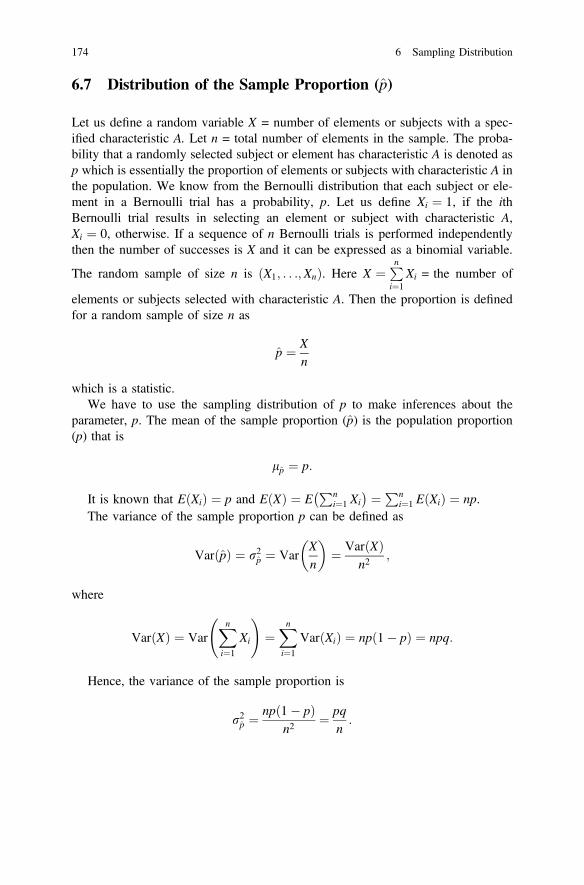
6.7 Distribution of the Sample Proportion (p)
Let us define a random variable X = number of elements or subjects with a spec-ified characteristic A. Let n = total number of elements in the sample. The proba-bility that a randomly selected subject or element has characteristic A is denoted asp which is essentially the proportion of elements or subjects with characteristic A inthe population. We know from the Bernoulli distribution that each subject or ele-ment in a Bernoulli trial has a probability, p. Let us define Xi ¼ 1, if the ithBernoulli trial results in selecting an element or subject with characteristic A,Xi ¼ 0, otherwise. If a sequence of n Bernoulli trials is performed independentlythen the number of successes is X and it can be expressed as a binomial variable.
The random sample of size n is X1; . . .;Xnð Þ. Here X ¼Pni¼1
Xi = the number of
elements or subjects selected with characteristic A. Then the proportion is definedfor a random sample of size n as
p ¼ Xn
which is a statistic.We have to use the sampling distribution of p to make inferences about the
parameter, p. The mean of the sample proportion (p) is the population proportion(p) that is
lp ¼ p:
It is known that EðXiÞ ¼ p and EðXÞ ¼ EPn
i¼1 Xi� � ¼Pn
i¼1 EðXiÞ ¼ np.The variance of the sample proportion p can be defined as
VarðpÞ ¼ r2p ¼ VarXn
¼ VarðXÞ
n2;
where
VarðXÞ ¼ VarXni¼1
Xi
!¼Xni¼1
VarðXiÞ ¼ npð1� pÞ ¼ npq:
Hence, the variance of the sample proportion is
r2p ¼np 1� pð Þ
n2¼ pq
n:
174 6 Sampling Distribution

The standard error of the sample proportion, p, is
rp ¼ffiffiffiffiffiffiffiffiffiffiffiffiffiffiffiffiffip 1� pð Þ
n
r¼
ffiffiffiffiffipqn
r:
For large sample size (n� 30; np[ 5; nq[ 5), the sample proportion (p) hasapproximately a normal distribution with mean lp ¼ p and a variance r2p ¼ pq=nthat is
p�N p;pqn
� �;
Z ¼ p� pffiffiffiffipqn
p �Nð0; 1Þ:
Example 6.10 Let us suppose that the proportion of under 5 children with under-weight for their height is 17%. If a sample of 50 under 5 children is selected atrandom, find the probability that
1. the proportion of children in the sample will be underweight for their height isgreater than 0.3, and
2. the proportion of children in the sample will be underweight for their height isbetween 0.1 and 0.2.
SolutionThe sample size is n = 50 which is greater than 30 and we may use the CentralLimit Theorem to obtain the sampling distribution characteristics of proportion. Thepercentage of underweight children for their height is 17% which means that theproportion of underweight children for their height is p ¼ 0:17.
Hence, the mean, variance, and standard error of p are
lp ¼ p ¼ 0:17;
r2p ¼pð1� pÞ
n¼ 0:17� 0:83
50¼ 0:1411
50¼ 0:0028;
rp ¼ 0:0531:
The asymptotic distribution of the sample proportion using the Central LimitTheorem is standardized normal distribution as shown below
Z ¼ p� pffiffiffiffiffiffiffiffiffiffiffipð1�pÞ
n
q � Nð0; 1Þ:
Then the probability that the sample proportion of underweight children forheight greater than 0.3 is
6.7 Distribution of the Sample Proportion (p) 175
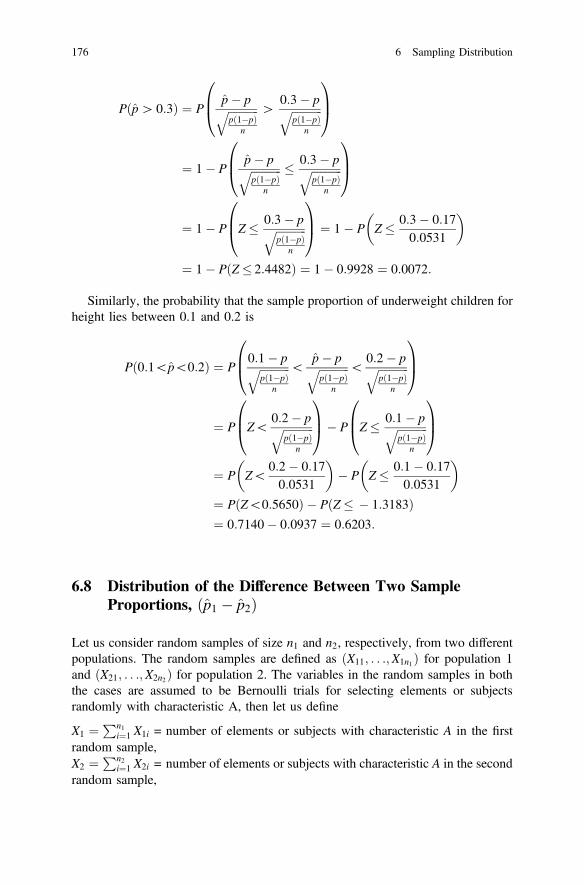
Pðp[ 0:3Þ ¼ Pp� pffiffiffiffiffiffiffiffiffiffiffip 1�pð Þ
n
q [0:3� pffiffiffiffiffiffiffiffiffiffiffi
p 1�pð Þn
q0B@
1CA
¼ 1� Pp� pffiffiffiffiffiffiffiffiffiffiffip 1�pð Þ
n
q � 0:3� pffiffiffiffiffiffiffiffiffiffiffip 1�pð Þ
n
q0B@
1CA
¼ 1� P Z� 0:3� pffiffiffiffiffiffiffiffiffiffiffip 1�pð Þ
n
q0B@
1CA ¼ 1� P Z� 0:3� 0:17
0:0531
¼ 1� P Z� 2:4482ð Þ ¼ 1� 0:9928 ¼ 0:0072:
Similarly, the probability that the sample proportion of underweight children forheight lies between 0.1 and 0.2 is
Pð0:1\p\0:2Þ ¼ P0:1� pffiffiffiffiffiffiffiffiffiffiffi
p 1�pð Þn
q \p� pffiffiffiffiffiffiffiffiffiffiffip 1�pð Þ
n
q \0:2� pffiffiffiffiffiffiffiffiffiffiffi
p 1�pð Þn
q0B@
1CA
¼ P Z\0:2� pffiffiffiffiffiffiffiffiffiffiffi
p 1�pð Þn
q0B@
1CA� P Z� 0:1� pffiffiffiffiffiffiffiffiffiffiffi
p 1�pð Þn
q0B@
1CA
¼ P Z\0:2� 0:170:0531
� P Z� 0:1� 0:17
0:0531
¼ P Z\0:5650ð Þ � P Z� � 1:3183ð Þ¼ 0:7140� 0:0937 ¼ 0:6203:
6.8 Distribution of the Difference Between Two SampleProportions, p1 � p2ð Þ
Let us consider random samples of size n1 and n2, respectively, from two differentpopulations. The random samples are defined as X11; . . .;X1n1ð Þ for population 1and X21; . . .;X2n2ð Þ for population 2. The variables in the random samples in boththe cases are assumed to be Bernoulli trials for selecting elements or subjectsrandomly with characteristic A, then let us define
X1 ¼Pn1
i¼1 X1i = number of elements or subjects with characteristic A in the firstrandom sample,X2 ¼
Pn2i¼1 X2i = number of elements or subjects with characteristic A in the second
random sample,
176 6 Sampling Distribution

p1 = proportion of elements of type (A) in the first population,p2 = proportion of elements of type (A) in the second population.
We are interested in comparing p1 and p2, or equivalently, making inferencesabout p1 − p2. Let us assume that we independently select the random samples ofsize n1 from the first population and another random sample of size n2 from thesecond population, then
p1 ¼ X1n1
= sample proportion of elements or subjects with characteristic A in ran-dom sample 1,p2 ¼ X2
n2= sample proportion of elements or subjects with characteristic A in ran-
dom sample 2, andp1 � p2 = difference between sample proportions.
The Sampling Distribution of p1 � p2The mean of the difference between sample proportions p1 � p2ð Þ is
lp1�p2 ¼ p1 � p2:
We can show that
EðX1iÞ ¼ p1 and EðX1Þ ¼ EXn1i¼1
X1i
!¼Xn2i¼1
EðX1iÞ ¼ n1p1;
and
EðX2iÞ ¼ p2 and EðX2Þ ¼ EXn2i¼1
X2i
!¼Xn2i¼1
EðX2iÞ ¼ n2p2:
Hence
lp1�p2 ¼ E p1 � p2ð Þ ¼ EX1
n1� X2
n2
¼ EðX1Þ
n1� E X2ð Þ
n2¼ p1 � p2:
The variance of the difference between two sample proportions where randomsamples are drawn independently is
Varðp1 � p2Þ ¼ r2p1�p2 ¼ VarX1
n1� X2
n2
¼ VarðX1Þ
n21þ VarðX2Þ
n22;
6.8 Distribution of the Difference Between Two Sample Proportions, p1 � p2ð Þ 177
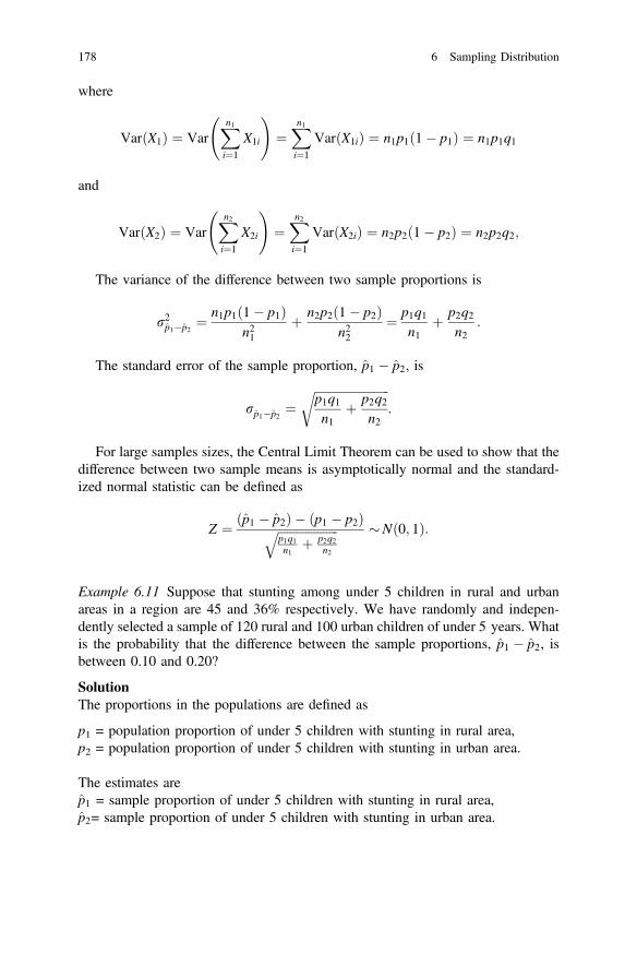
where
VarðX1Þ ¼ VarXn1i¼1
X1i
!¼Xn1i¼1
VarðX1iÞ ¼ n1p1ð1� p1Þ ¼ n1p1q1
and
VarðX2Þ ¼ VarXn2i¼1
X2i
!¼Xn2i¼1
VarðX2iÞ ¼ n2p2ð1� p2Þ ¼ n2p2q2;
The variance of the difference between two sample proportions is
r2p1�p2 ¼n1p1 1� p1ð Þ
n21þ n2p2 1� p2ð Þ
n22¼ p1q1
n1þ p2q2
n2:
The standard error of the sample proportion, p1 � p2, is
rp1�p2 ¼ffiffiffiffiffiffiffiffiffiffiffiffiffiffiffiffiffiffiffiffiffiffiffiffiffip1q1n1
þ p2q2n2
r:
For large samples sizes, the Central Limit Theorem can be used to show that thedifference between two sample means is asymptotically normal and the standard-ized normal statistic can be defined as
Z ¼ ðp1 � p2Þ � ðp1 � p2Þffiffiffiffiffiffiffiffiffiffiffiffiffiffiffiffiffiffiffiffip1q1n1
þ p2q2n2
q �Nð0; 1Þ:
Example 6.11 Suppose that stunting among under 5 children in rural and urbanareas in a region are 45 and 36% respectively. We have randomly and indepen-dently selected a sample of 120 rural and 100 urban children of under 5 years. Whatis the probability that the difference between the sample proportions, p1 � p2, isbetween 0.10 and 0.20?
SolutionThe proportions in the populations are defined as
p1 = population proportion of under 5 children with stunting in rural area,p2 = population proportion of under 5 children with stunting in urban area.
The estimates arep1 = sample proportion of under 5 children with stunting in rural area,p2= sample proportion of under 5 children with stunting in urban area.
178 6 Sampling Distribution
The population proportions given are p1 = 0.45 for rural area and p2 = 0.36 forurban area and sample size for rural and urban areas are n1 ¼ 120 and n2 ¼ 100,respectively. The difference between sample proportions is
lp1�p2 ¼ p1 � p2 ¼ 0:45� 0:36 ¼ 0:09
The variance and standard error of the difference between two sample estimatescan also be obtained as shown below
r2p1�p2 ¼p1 � q1
n1þ p2 � q2
n2
¼ 0:45� 0:55120
þ 0:36� 0:64100
¼ 0:0021þ 0:0023
¼ 0:0044:
The standard error of the difference between two sample proportions is
rp1�p2 ¼ffiffiffiffiffiffiffiffiffiffiffiffiffiffiffiffiffiffiffiffiffiffiffiffiffiffiffiffiffiffiffiffiffiffiffiffip1 � q1
n1þ p2 � q2
n2
r¼
ffiffiffiffiffiffiffiffiffiffiffiffiffiffi0:0044
p
¼ 0:0663:
To find the probability of the difference between the sample proportions,p1 � p2, between 0.10 and 0.20, we follow the steps shown below:
Pð0:10\p1 � p2\0:20Þ ¼ P0:10� ðp1 � p2Þffiffiffiffiffiffiffiffiffiffiffiffiffiffiffiffiffiffiffiffi
p1q1n1
þ p2q2n2
q \p1 � p2 � ðp1 � p2Þffiffiffiffiffiffiffiffiffiffiffiffiffiffiffiffiffiffiffiffi
p1q1n1
þ p2q2n2
q \0:20� ðp1 � p2Þffiffiffiffiffiffiffiffiffiffiffiffiffiffiffiffiffiffiffiffi
p1q1n1
þ p2q2n2
q0B@
1CA
¼ P0:10� ðp1 � p2Þffiffiffiffiffiffiffiffiffiffiffiffiffiffiffiffiffiffiffiffi
p1q1n1
þ p2q2n2
q \Z\0:20� ðp1 � p2Þffiffiffiffiffiffiffiffiffiffiffiffiffiffiffiffiffiffiffiffi
p1q1n1
þ p2q2n2
q0B@
1CA
¼ P0:10� 0:100:0663
\Z\0:20� 0:100:0633
¼ P 0\Z\1:5798ð Þ¼ P Z\1:5798ð Þ � P Z� 0ð Þ¼ 0:9429� 0:5 ¼ 0:4429:
6.8 Distribution of the Difference Between Two Sample Proportions, p1 � p2ð Þ 179
6.9 Chi-Square Distribution (v2—Distribution)
We learned about the standardized normal distribution in Chap. 5. Let us consider arandom sample of size n, ðX1; . . .;XnÞ, from a normal population with mean l andvariance r2 expressed as X�Nðl; r2Þ then the standardized normal variable isdefined by
Z ¼ X � lr
�Nð0; 1Þ:
The random sample is drawn independently from the identical normal distri-bution X �Nðl; r2Þ. This implies that Xi; i ¼ 1; . . .; n is drawn independently fromthe population such that Xi �Nðl; r2Þ that is each variable in the random samplehas an identical distribution. Then a chi-square is defined as the sum of squaredstandardized normal variables for known l and r2 as shown below
v2 ¼Xni¼1
Z2i ;
where this is called chi-square statistic with n degrees of freedom and is denoted byv2n.
It is not practical to use chi-square in situations when the population mean andthe variance are not known. Another problem with the chi-square statistic describedabove is that the normality assumption may not hold in many instances. Let usdiscuss these situations. If the mean and the variance of the normal population fromwhere the random sample is drawn are not known then we can define the followingcomponents of a chi-square
v2n ¼Xni¼1
Xi � lr
2
¼Xni¼1
Xi � �Xð Þ2 þð�X � lÞ2r2
" #
¼Xni¼1
Xi � �Xð Þ2r2
þ nð�X � lÞ2r2
¼Xni¼1
Xi � �Xð Þ2r2
þ ð�X � lÞ2r2=n
As we have shown earlier that �X�Nðl; r2=nÞ and �X�lr=ffiffin
p �Nð0; 1Þ then it followsthat
180 6 Sampling Distribution
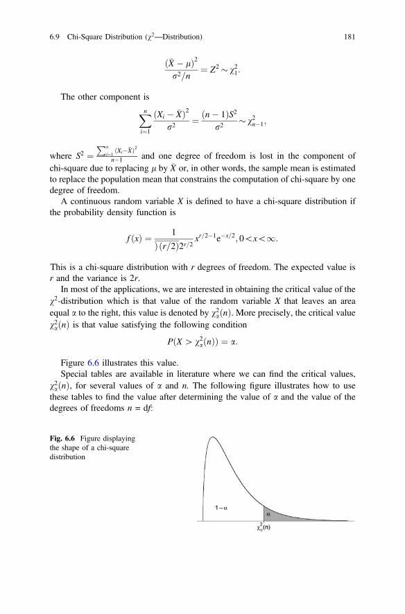
�X � lð Þ2r2=n
¼ Z2 � v21:
The other component is
Xni¼1
Xi � �Xð Þ2r2
¼ ðn� 1ÞS2r2
� v2n�1;
where S2 ¼Pn
i¼1Xi��Xð Þ2
n�1 and one degree of freedom is lost in the component ofchi-square due to replacing l by �X or, in other words, the sample mean is estimatedto replace the population mean that constrains the computation of chi-square by onedegree of freedom.
A continuous random variable X is defined to have a chi-square distribution ifthe probability density function is
f ðxÞ ¼ 1
Þðr=2Þ2r=2 xr=2�1e�x=2; 0\x\1:
This is a chi-square distribution with r degrees of freedom. The expected value isr and the variance is 2r.
In most of the applications, we are interested in obtaining the critical value of thev2-distribution which is that value of the random variable X that leaves an areaequal a to the right, this value is denoted by v2aðnÞ. More precisely, the critical valuev2aðnÞ is that value satisfying the following condition
PðX[ v2aðnÞÞ ¼ a:
Figure 6.6 illustrates this value.Special tables are available in literature where we can find the critical values,
v2aðnÞ, for several values of a and n. The following figure illustrates how to usethese tables to find the value after determining the value of a and the value of thedegrees of freedoms n = df:
Fig. 6.6 Figure displayingthe shape of a chi-squaredistribution
6.9 Chi-Square Distribution (v2—Distribution) 181
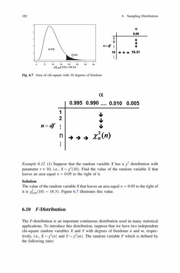
Example 6.12 (1) Suppose that the random variable X has a v2 distribution withparameter r = 10, i.e., X� v2ð10Þ. Find the value of the random variable X thatleaves an area equal a ¼ 0:05 to the right of it.
SolutionThe value of the random variable X that leaves an area equal a ¼ 0:05 to the right ofit is v20:05ð10Þ ¼ 18:31. Figure 6.7 illustrates this value.
6.10 F-Distribution
The F-distribution is an important continuous distribution used in many statisticalapplications. To introduce this distribution, suppose that we have two independentchi-square random variables X and Y with degrees of freedoms n and m, respec-tively, i.e., X � v2ðnÞ and Y � v2ðmÞ. The random variable F which is defined bythe following ratio:
Fig. 6.7 Area of chi-square with 10 degrees of freedom
182 6 Sampling Distribution

F ¼ X=nY=m
has an F-distribution with parameters n and m, and we write F�Fðn;mÞ. The F-distribution is characterized by two parameters n and m and we can find theprobabilities of F on the basis of these degrees of freedom. In general, the F-distribution is used extensively to compare sample variances and it has a wide rangeof applications to compare two or more samples.
The sampling distribution of F is the probability density function of the ratio
F ¼ X=nY=m where X � v2ðnÞ and. Y � v2ðmÞ, n and m are degrees of freedom,
respectively. The sampling distribution of F is given by the density function
gðf Þ ¼ Þ ðnþmÞ=2 n=mð Þn=2Þ n=2Þm=2
f n=2�1
1þ nf =mð ÞðnþmÞ=2 ; 0\f\1:
In most of the applications, we are interested in obtaining the critical value ofF which is that value of the random variable F that leaves an area equal a to theright, this value is denoted by Faðn;mÞ. More precisely, the critical value Faðn;mÞis that value satisfying the following condition:
PðF[Faðn;mÞÞ ¼ a:
Figure 6.8 illustrates this value.A special table is available in literature where we can find the critical value
Faðn;mÞ for several values of n, m, and a. The following figure illustrates how touse these tables to find the critical value Faðn;mÞ after determining the value of aand the values of the degrees of freedoms n and m:
Fig. 6.8 Figure displayingthe shape of an F-distribution
6.10 F-Distribution 183

Example 6.13 Suppose that the random variable F has an F-distribution with pa-rameters n = 5 and m = 10, i.e., F�Fð5; 10Þ. Find the value of the random vari-able F that leaves an area equal a ¼ 0:05 to the right of it.
SolutionThe value of the random variable F that leaves an area equal a ¼ 0:05 to the right ofit is F0:05ð5; 10Þ ¼ 3:33. Figure 6.9 illustrates this value.
6.11 Summary
In this chapter, the concepts of sampling distribution are introduced. The meaningof a sampling distribution is illustrated with examples in order to provide the userswith fundamental concepts in a step-by-step procedure. The sampling distributionsof mean for both small and large samples are discussed. The underlying assump-tions about the distributions from which the samples are drawn and about thepopulation variance are also highlighted. Similarly, the sampling distributions of
Fig. 6.9 Figure displaying F-distribution with (5, 10) degrees of freedom
184 6 Sampling Distribution

difference between two means along with the underlying assumptions about thepopulations are shown with examples. The sampling distributions of sample pro-portion and difference between two proportions are discussed with examples. Thesampling distributions included in this chapter are normal, t, chi-square, and F-distributions.
Exercises
6:1 Suppose that a population is comprised of 10 elements. The elements of thepopulation are X1 ¼ 10;X2 ¼ 7;X3 ¼ 15; X4 ¼ 16;X5 ¼ 5;X6 ¼ 11;X7 ¼14; X8 ¼ 8;X9 ¼ 15;X10 ¼ 11.In other words, the population size is N = 10. A sample of size n = 2 is to bedrawn randomly.
(i) How many samples can be drawn with replacement?(ii) How many samples can be drawn without replacement?(iii) Find the sample means of all possible samples that can be drawn
without replacement.(iv) Find the population mean, l.(v) Find the population variance, r2.(vi) Find the expected value of the sample mean, �X; l�X :
(vii) Find the variance of the sample mean, �X, r2�X .(viii) Using the above results, are the following statements true?
(a) l�X ¼ l;(b) r2�X ¼ r2
n .
6:2 Suppose X is distributed as normal with population mean 10 and populationvariance 4. For a random sample of size 9, what is the sampling distributionof the sample mean, �X? Also, define the standard normal variate using thegiven information.
6:3 Let us consider a non-normal population with mean 150 and variance 25.How can you find the sampling distribution of the sample mean for a randomsample of size n = 100? What are the underlying preconditions for theasymptotic sampling distribution?
6:4 Find the following values for m ¼ 14:
(a) (i) t0:05,(ii) t0:95,(iii) t0:01,(iv) t0:025, and(v) t0:001.
6:5 Find the following probabilities:
(i) Pð�1:476\T\1:476Þ for m ¼ 5,(ii) Pð�1:7959\T\1:7959Þ for m ¼ 11,
6.11 Summary 185

(iii) Pð�2:1009\T\2:1009Þ for m ¼ 18,(iv) PðT\� 2:500Þ for m ¼ 23, and(v) PðT [ 2:500Þ for m ¼ 23.
6:7 Suppose that the variable X be a normal distribution with population mean 15and standard deviation 3.5. A study is conducted with sample size n = 70.
(i) What is the sampling distribution of the sample mean �X?(ii) Find the probability Pð�X\17Þ.(iii) Find the probability Pð�X[ 12Þ.(iv) Find the probability Pð12\�X\17Þ.
6:8 Let X be distributed with population mean 40 and variance 16 where thepopulation is not normal. If a random sample of size 100 is drawn from thepopulation then find:
(i) the sampling distribution of the sample mean �X,(ii) the probability Pð�X\25Þ,(iii) the probability Pð�X[ 45Þ,(iv) the probability Pð30\�X\50Þ.
6:9 Let the variable X be normal with population mean 125 but the populationvariance is unknown. A random sample of size 16 is drawn from the pop-ulation and the sample variance is obtained where the sample variance s2 is81. Then find:
(i) the sampling distribution of the sample mean �X,(ii) the probability Pð�X\100Þ,(iii) the probability Pð�X[ 150Þ,(iv) the probability Pð90\�X\150Þ.
6:10 The population mean, and variance of a characteristic, X, of two groups ofindividuals are l1 ¼ 25; r21 ¼ 9 for group 1 and l2 ¼ 31; r22 ¼ 12 for group2. In a study on the difference between two population means, the samplesizes for groups 1 and 2 are 100 and 150, respectively.
(i) Show the sampling distribution of the difference between two popu-lation means.
(ii) Find the probability Pð�X1 � �X2 [ 10Þ.(iii) Find the probability Pð�X1 � �X2\5Þ.(iv) Find the probability Pð2\�X1 � �X2\7Þ.
6:11 Suppose that the population mean and variance of a variable, X, for groupA arel1 ¼ 10 and r21 ¼ 5 and for group B are l2 ¼ 12 and r22 ¼ 7. A study isconducted to find the difference between two population means. The samplesizes for groups A and B are 11 and 14, respectively.
186 6 Sampling Distribution

(i) What is the sampling distribution of �X1 � �X2?(ii) Find the probability Pð�X1 � �X2 [ 4Þ.(iii) Find the probability Pð�X1 � �X2\1Þ.(iv) Find the probability Pð1\�X1 � �X2\4Þ.
6:12 In a population, the proportion of infants suffering from high fever during themonth of December in a community is believed to be 0.2. A random sampleof 100 infants is drawn randomly from the population.
(i) What is the sampling distribution of sample proportion for largesample size?
(ii) Find the probability that more than 30% of the infants suffered fromhigh fever.
(iii) What is the probability that less than 10% of the infants suffered fromhigh fever.
(iv) What is the probability that the proportion of infants suffered fromhigh fever lies between 0.1 and 0.3?
6:13 Two independent samples are drawn from male and female populations withproportion of a complication associated with a chronic disease. The pro-portion of complication among the male population is 0.25 and among thefemale population is 0.20. The sample size for male is 150 and for female is175.
(i) What is the sampling distribution of the difference between sampleproportions for male and female?
(ii) Find the probability that the difference between male and femaleproportions is less than 1%.
(iii) Find the probability that the probability of a difference between maleand female proportions having complications greater than 10%.
(iv) What is the probability that the difference between proportions of maleand female suffering from complications lies between 0.03 and 0.07?
6.11 Summary 187

Chapter 7Estimation
7.1 Introduction
Statistical inference refers to the methods by which we arrive at a conclusion abouta population on the basis of the information contained in a sample drawn from thatpopulation. The sample is drawn from a population randomly and hence a randomsample of size n considers a method of selecting a sample with predeterminedprobability. We have discussed about the sampling distribution of statistics inChap. 6 and it is shown that a sampling distribution provides the underlyingprobability distribution of the statistics by which we try to generalize for popula-tion. As the sampling distribution is based on all the possible samples from apopulation of size N, the expected value, variance, and other population charac-teristics can be obtained theoretically from the statistics of a random sample.Statistical inference is comprised of two broad components: (i) estimation and(ii) test of hypothesis. Estimation refers to the methods of finding the value ofstatistic from a sample corresponding to its population value such that it satisfiessome good properties to represent a parameter. On the other hand, once we obtain avalue to estimate the corresponding population value or parameter, it is needed toknow whether the sample value used as an estimate is close to the true value. Thisissue is of great importance in statistics and there are various techniques to makecomment or to make decision about generalizing the estimates obtained by esti-mating parameters for the population as a whole. As the estimates are obtained fromrandomly drawn samples, it is likely that the values we consider to be populationcharacteristics may differ from the true value. It means that although drawn from thepopulation, a sample estimate may not be exactly equal to the correspondingparameter. Hence, as a statistician or biostatistician, it is necessary to provideprocedures to make decision about the population values such that with the help ofunderlying sampling distribution, we may come up with decision about the popu-lation value where underlying probability distribution of statistic or sampling dis-tribution plays an important role.
© Springer Nature Singapore Pte Ltd. 2018M. A. Islam and A. Al-Shiha, Foundations of Biostatistics,https://doi.org/10.1007/978-981-10-8627-4_7
189

Let us consider two examples here to highlight the role of estimation and test inbiostatistics. In the first example, let us consider a study to find the mean duration ofbreastfeeding in a population. A random sample ðX1; . . .;XnÞ is considered withX� f ðx; l;r2Þ and the sample observations are X1 ¼ x1; . . .;Xn ¼ xn. The samplemean of the duration is found to be �x. Let the sampling distribution of �X be knownor assumed and we also know that Eð�XÞ ¼ l where l is the population mean of thepopulation from which the random sample is drawn. Then the statistical procedureto establish �x as an estimate of l is called a method of estimation. Once we obtainan estimate for l, the next step is to confirm whether the population mean is aspecified value, say l ¼ l0. Based on the sample mean and also using the samplingdistribution of the sample mean, we may not reject or reject the hypothesis that themean duration of breastfeeding in the population is l ¼ l0.This is a typical problemof test of hypothesis. In other words, a test of hypothesis is used to generalize thefindings from the sample estimates for the population from where the sample isdrawn randomly. In a study on old age population, the proportions of males andfemales suffering from high blood pressure are estimated. The sample values orstatistics are p1 and p2 and the corresponding parameters are p1 and p2, respectively.In this case, p1 and p2 may be used to estimate the population values or parametersp1 and p2. The estimates are computed from sample values as p1¼ X1
n1and p2 ¼ X2
n2where X1 and X2 are number of males and females with high blood pressure, andn1 and n2 are number of males and females in the survey. The sample values orstatistics of proportions with high blood pressure among males and females are usedto represent the population values. As the sample is drawn randomly, we can showthat expected values of the sample proportions are equal to the parameters. The waythe sample values are chosen to estimate the parameters is a technique of estima-tion. Once we have the estimates, let us test for the hypothesis that proportion ofmales and females suffering from high blood pressure are the same in the popu-lation. If not same, then either males or females may suffer from high bloodpressure at a higher proportion. Using the sampling distribution of differencebetween sample proportions, we can come up with a decision regardingnon-rejection or rejection of the hypothesis. The means to test the difference orequality of sample proportions is performed by using a method of test of hypoth-esis. We try to arrive at a correct decision about the population characteristic on thebasis of a sample value known as estimate and a test of hypothesis.
7.2 Estimation
Let us assume that some characteristics of the elements in a population be repre-sented by a random variable X with probability density f ðx; hÞ where the form of theprobability density function is assumed known except that it contains an unknownparameter, h. If h were known, the density function would be completely specified,and there would be no need to make inferences about it. We assume that the values
190 7 Estimation

ðx1; . . .; xnÞ of a random sample ðX1; . . .;XnÞ from f ðx; hÞ can be observed. It isdesired to estimate the value of the unknown parameter, h.
This estimation can be made in two ways:
i. Point estimation: If some statistic, say �X, represents or estimates the unknownparameter, l, then �X is called a point estimator. A point estimate is a singlevalue such as �X ¼ �x used to estimate the corresponding population parameter.Hence, a point estimator is a statistic that represents the function of randomvariables of a random sample to represent or estimate an unknown parameterand any single value of the statistic or more specifically estimator in this caseused to estimate the parameter is a point estimate.
ii. Interval estimation: Let us define two statistics, L and U, where L < U such that(L, U) constitutes an interval for which the probability can be determined that itcontains the unknown parameter. An interval estimate consists of two numer-ical values defining a range of values that most likely includes the parameterbeing estimated with a specified degree of confidence.
There are two problems that we need to address in point estimation:
(i) to desire some means of obtaining a statistic to use as an estimator,(ii) to select criteria and techniques to define and find best estimator among many
possible estimators.
7.2.1 Methods of Finding Point Estimators
Let X1; . . .;Xn be a random sample from a population density or mass function,fXðx; hÞ, which is denoted as f ðx; hÞ in this book for simplicity, where the form ofthe density is known but the parameter is unknown. We need to find statistics,functions of observations to be used as estimator of the parameter.
Estimator and EstimateAny statistic is a function of observable random variables that is itself a randomvariable. The value of statistic that is used to estimate the parameter, say h, is calledthe estimator of the parameter h. Any specific value of the estimator from a sample
is called as estimate. Example: �X ¼Pn
i¼1Xi
n is an estimator of mean l and �x ¼Pn
i¼1xi
n is an estimate where X1 ¼ x1; . . .;Xn ¼ xn are the realizations of the variableby the sample observations. It may be noted here that the estimator, �X, is a randomvariable because it is a function of observable random variables X1; . . .;Xn and theestimate, �x, is a specific value of the function from the sample observations.
Sometimes, it is an easy task to find estimators, for example, estimating aparameter with its sample analogue is usually reasonable. In particular, the samplemean is a good estimate for the population mean. In more complicated models, weneed to use a more methodical way. The most extensively used techniques of
7.2 Estimation 191

estimating parameters are: (i) method of moments, (ii) method of maximum like-lihood, and (iii) method of least squares. We will illustrate the first two methodsvery briefly in this section and the third method will be discussed in Chap. 9.
Method of Moments
The method of moments is the oldest technique for estimating parameters of aprobability distribution. This method is simple to use and almost always yieldssome sort of estimate. However, method of moments sometimes provides estimatorthat needs improvement. If other methods are intractable, method of moments canbe a good starting point.
Let ðX1; . . .;XnÞ be a sample from a population with probability density function(pdf) or probability mass function (pmf), fXðx; hÞ, then the method of momentsestimators is found by equating the first k sample moments to the correspondingk population moments if there are k parameters to be estimated, and solving theresulting system of simultaneous equations, we obtain the estimates. In other words,if there is a single parameter, then we have to use the first sample moment andequating with the first population moment. Similarly, if there are two parameters,we can use the first two sample and population moments.
If there are k parameters, then we need first k raw sample and populationmoments as defined below:
SampleMoments PopulationMoments
m01 ¼
Pn
i¼1xi
n l01 ¼ EðXÞm0
2 ¼Pn
i¼1x2i
n l02 ¼ EðX2Þ... ..
.
m0k ¼
Pn
i¼1xki
n l0k ¼ EðXkÞ
Then the estimates are obtained for the k parameters by solving the followingsimultaneous equations:
~l01 ¼ m01;
~l02 ¼ m02;
..
.
~l0k ¼ m0k:
Example 7.1 Let ðX1; . . .;XnÞ be a random sample from a Poisson distribution withparameter k, then
l01 ¼ EðXÞ ¼ k
192 7 Estimation

and
m01 ¼
Pni¼1 xin
¼ �x:
Hence, the method of moments estimate for k is
~k ¼ �x:
Method of Maximum Likelihood
The concept of a joint distribution arises if we draw a random sample of size n froma multivariate population. If a sample of size n is drawn from a populationsimultaneously, we need to define the underlying joint probability forX1 ¼ x1; . . .;Xn ¼ xn. The joint probability density or mass function is
f ðx1; . . .; xn; hÞ
where this joint distribution expresses the probability distribution for the randomsample values X1 ¼ x1; . . .;Xn ¼ xn. Here h is unknown. The joint distributioninvolves not only parameters of a univariate distribution but also parameters forassociation or correlation between random sample variables X1; . . .;Xn. However, ifthe random variables X1; . . .;Xn are independent then there is a simple relationshipbetween joint distribution and univariate distributions as shown below
f ðx1; . . .; xn; hÞ ¼ f ðx1; hÞ . . . f ðxn; hÞ:It means that the joint distribution is the multiplication of marginal probabilities
under independence of the random variables.It is stated in case of a random sample that the joint probability of X1 ¼
x1; . . .;Xn ¼ xn is of concern in a joint distribution and once the parameter isknown, then the probabilities of observed values for n random variables can beobtained. Now if we consider that for a random sample the values of variables areknown, i.e., the sample observations x1; . . .; xn are given, then what the likelyestimate of h would be for which the probability of h is maximum. This idea leadsto the concept of the likelihood function.
The concept of the theory of likelihood is not only the most popular but also themost useful technique with very important properties for deriving estimates ofparameters of any probability distribution. If X1; . . .;Xn are independently andidentically distributed random variables with pdf or pmf f ðx; hÞ then the likelihoodfunction is defined by
L h x1; . . .; xnjð Þ ¼Yni¼1
f xi hjð Þ:
The left-hand side defines the probability of the likely values of parameter forgiven observed values x1; . . .; xn of a random sample and the right-hand side is the
7.2 Estimation 193

joint probability of X1 ¼ x1; . . .;Xn ¼ xn for a given h. The left-hand side is equal tothe right-hand side only when the random variables X1; . . .;Xn independently andidentically distributed. It may be noted here that for each sample point x, let there bea parameter value at which L h xjð Þ is expected to attain its maximum as a function ofh, if x is held fixed. A maximum likelihood estimator (MLE) of the parameter hbased on a sample X1; . . .;Xn is h Xð Þ or simply h.
If the likelihood function is differentiable in h, then the MLE is obtained bysolving the following equation:
ddh
L h x1; . . .; xnjð Þ ¼ 0:
The likelihood function for k parameters, h1; . . .; hk is
L h1; . . .; hk x1; . . .; xnjð Þ ¼Yni¼1
f xi h1; . . .; hkjð Þ
and the maximum likelihood equations are
ddh1
L h1; . . .; hk x1; . . .; xnjð Þ ¼ 0;
..
.
ddhk
L h1; . . .; hk x1; . . .; xnjð Þ ¼ 0:
The maximum likelihood estimates are obtained by solving the maximumlikelihood equations and the estimates are denoted by h1; . . .; hk .
To confirm maximization, we need to find the second derivatives of the likeli-hood functions and negative value of the second derivatives indicate that theestimates provide maximum likelihood. The second derivatives are
d2
dh21L h1; . . .; hk x1; . . .; xnjð Þ\0;
..
.
d2
dh2kL h1; . . .; hk x1; � � � ; xnjð Þ\0:
It is noteworthy that instead of the likelihood functions, we can use thelog-likelihood functions for making the equations more convenient to obtain thesame solutions. The log-likelihood function for k parameters, h1; . . .; hk is
ln L h1; . . .; hk x1; . . .; xnjð Þ ¼Xni¼1
ln f xi h1; . . .; hkjð Þ
194 7 Estimation

and the maximum log-likelihood equations are
ddh1
ln L h1; . . .; hk x1; . . .; xnjð Þ ¼ 0;
..
.
ddhk
ln L h1; . . .; hk x1; . . .; xnjð Þ ¼ 0:
and the second derivatives are
d2
dh21ln L h1; . . .; hk x1; . . .; xnjð Þ\0;
..
.
d2
dh2kln L h1; . . .; hk x1; . . .; xnjð Þ\0:
Some important properties of the maximum likelihood estimators are summa-rized here: (i) Invariance Property: If h is a maximum likelihood estimator of h, thengðhÞ is the maximum likelihood estimator of gðhÞ where gðhÞ is a function of h;(ii) Asymptotically Unbiased: The maximum likelihood estimator, h, is asymptot-ically unbiased such that EðhÞ ! h as n ! 1 but not necessarily exactly unbiased;(iii) Consistency: Under certain regularity conditions, the maximum likelihoodestimator h is a consistent estimator of h; and (iv) Normality: Under regularityconditions, the maximum likelihood estimator h is asymptotically normally dis-tributed with mean h.
Example 7.2 Let X1; . . .;Xn be iid Bernoulli (p).The likelihood function is
L p xj 1; . . .; xn� � ¼Yn
i¼1
pxi 1� pð Þ1�xi
¼ py 1� pð Þn�y; y ¼X
xi
ln L p xj 1; . . .; xn��� � ¼ y ln pþ n� yð Þ ln 1� pð Þ
d ln LðpÞdp
¼ yp� n� y
1� pð Þ ¼ 0
or bp ¼ yn:
7.2.2 Interval Estimation
We have discussed about point estimation in the previous section. From pointestimation, it has been observed that a single value represents the parameter in pointestimation. The use of point estimation for generalizing the result from sample to
7.2 Estimation 195
population is relatively simple and convenient but it may not provide someimportant information regarding the extent of error associated with the point esti-mate. In other words, if a point estimate is accompanied by a measure of the extentof error associated with a point estimate then the reliability of an estimate becomesmore meaningful and the extent of confidence about the estimation can also beassigned to such estimation.
An interval estimate of h is an interval (L, U) containing the true value of h witha probability of 1� a where 1� a is called the confidence coefficient (level),L = lower limit of the confidence interval, and U = upper limit of the confidenceinterval. Hence, we can express the 100ð1� aÞ% two-sided confidence interval asP L� h�Uð Þ ¼ 1� a. Similarly, we can define the one-sided lower confidenceinterval as P L� hð Þ ¼ 1� a where L is the one-sided lower confidence limit for hand P h�Uð Þ ¼ 1� a where U is the one-sided upper confidence limit for h. It isimportant to remember that L and U are random variables, not h, hence the inter-pretation of confidence interval needs a very careful attention. As h remains con-stant which is a parameter, we can only interpret in terms of whether the parameterh is included in the interval or not. Furthermore, the interval constructed from asingle sample cannot provide the probability statement but it has to be interpreted inreference to the construction of similar intervals for each sample repeated a verylarge number of times with same sample size from the same population. In otherwords, the sampling distribution of the pivotal quantity provides the necessarybackground for both construction and interpretation of confidence interval.
The most extensively used method of finding confidence interval is the PivotalQuantity Method. In addition, sometimes other statistical methods are alsoemployed. Another method, known as the confidence sets, is also used for con-structing confidence intervals. The most commonly used technique, the PivotalQuantity Method, is highlighted in this chapter.
Pivotal Quantity Method: Let us consider a random sample X1; . . .;Xn of sizen from the population density X � f ðx; hÞ and let Q ¼ qðX1; . . .;Xn; hÞ where Q is afunction of random variables X1; . . .;Xn and parameter h such that the samplingdistribution of Q does not depend on h then Q is defined as a pivotal quantity.Based on the pivotal quantity, we obtain the confidence intervals using the samplingdistribution of pivotal quantity. Let us define the following probability with lowerand upper limits or bounds for the pivotal quantity, Q ¼ qðX1; . . .;Xn; hÞ:
P q1ðX1; . . .;Xn; hÞ\Q\q2ðX1; . . .;Xn; hÞ½ �\1� a
then after some algebraic manipulation, we arrive at the confidence interval for theparameter with confidence coefficient 1� a as
P LðX1; . . .;Xn; hÞ\h\UðX1; . . .;Xn; hÞ½ �\1� a;
where L and U are lower and upper bounds, limits or lower and upper end points ofthe confidence interval. The lower and upper limits are computed from a sampleX1 ¼ x1; . . .;Xn ¼ xn
196 7 Estimation

L ¼ lðx1; . . .; xnÞ andU ¼ uðx1; . . .; xnÞ:
Some examples of pivotal quantities are shown below:
(i) Z ¼ �X�lr=ffiffin
p where Z� Nð0; 1Þ does not depend on l,
(ii) T ¼ �X�lS=ffiffin
p where T � tn�1 does not depend on l,
(iii) v2¼Pni¼1
Xi��Xð Þ2r2 ¼ ðn�1ÞS2
r2 � v2n�1 does not depend on r2, and (Fig. 7.1).
(iv) F ¼ X=ðn�1ÞY=ðm�1Þ � Fðn� 1;m� 1Þ where X� v2ðn� 1Þ; Y � v2ðm� 1Þ,
v2ðn� 1Þ ¼Xn
i¼1
Xi � �Xð Þ2r2X
¼ ðn� 1ÞS2Xr2X
� v2n�1 and
v2ðm� 1Þ ¼Xm
i¼1
Yi � �Yð Þ2r2Y
¼ ðm� 1ÞS2Yr2Y
� v2m�1
,
and it is seen that F does not depend on the parameters r2X and r2Y .
All these statistics satisfy the conditions required for pivotal quantity, hence, canbe employed to construct confidence intervals (Fig. 7.2).
7.2.3 Estimation of Population Mean lð Þ
In this section, we are interested in estimating the parameters of population such asthe mean of a certain population lð Þ. Let us define the population and samplecharacteristics as displayed below.
Fig. 7.1 Chi-square distribution
7.2 Estimation 197

Population Sample
Population size = N Sample size = n
Population values: X1; . . .;XN Sample values: X1; . . .;Xn
Population mean: l ¼PN
i¼1Xi
NSample mean: �X ¼
Pn
i¼1Xi
n
Population variance: r2 ¼PN
i¼1Xi�lð Þ2N Sample variance: S2 ¼
Pn
i¼1Xi�Xð Þ2
n�1
(i) Point Estimation of l
A point estimate of the mean is a single number used to estimate (or approxi-mate) the true value of l. Let us consider a random sample of size n, X1; . . .;Xn withX� Nðl; r2Þ. Then the sample mean of the random sample is �X ¼ 1
n
Pni¼1 Xi and
the sample mean computed from observations X1 ¼ x1; . . .;Xn ¼ xn is�x ¼ 1
n
Pni¼1 xi. It should be noted here that �X is a variable and �x is a value of the
variable �X from observations of the random sample. We obtain the estimator of thesample mean using the maximum likelihood method as shown below.
The likelihood function is
Lðl; r2; x1; . . .; xnÞ ¼Yni¼1
f ðxi;l; r2Þ
¼ 1
2pr2ð Þn=2Yni¼1
e�1
2r2xi�lð Þ2
¼ 1
2pr2ð Þn=2e� 1
2r2
Pni¼1
xi�lð Þ2
and the log-likelihood function can be shown as
Fig. 7.2 F-distribution
198 7 Estimation

ln L l; r2; x1; . . .; xn� � ¼ � n
2ln 2pr2� �� 1
2r2Xni¼1
xi � lð Þ2:
The maximum likelihood estimate of the population mean, l, is found bysolving the equation
@ ln L@l
¼ � 22r2
Xni¼1
ðxi � lÞð�1Þ ¼ 1r2Xni¼1
ðxi � lÞ ¼ 0
and the maximum likelihood estimate is
l ¼Pn
i¼1 xin
:
The estimator of the population for the random sample is denoted as l ¼ �X ¼Pn
i¼1Xi
n which is a random variable.
(ii) Confidence Interval (Interval Estimate) of l
An interval estimate of l is an interval (L, U) containing the true value of l witha probability of 1� a where 1� a = is called the confidence coefficient, L = lowerlimit of the confidence interval, and U = upper limit of the confidence interval. The100ð1� aÞ% confidence interval is P L� l�Uð Þ ¼ 1� a where L and U arevariables and different samples will produce different values of end points ofconfidence interval L and U. From any sample data, we can find L = l and U = u.
A. Let us consider the case when r is known.
If X1; . . .;Xn is a random sample of size n from a normal distribution with meanl and known variance r2, then let us define the pivotal quantity
Z ¼�X � lr=
ffiffiffin
p :
This statistic is independent of parameters l and r and Z is a variable withprobability distribution N (0, 1). The probability of 1� a can be obtained from thefollowing interval:
Pðza=2\Z\z1�a=2Þ ¼ 1� a:
Here 1� a is the confidence coefficient. We know that Z is a function of sampleobservations and population mean and it can be shown in the interval
7.2 Estimation 199

P za=2\Z ¼�X � lr=
ffiffiffin
p \z1�a=2
� �¼ 1� a
¼ P za=2 � r=ffiffiffin
p\�X � l\z1�a=2 � r=
ffiffiffin
p� � ¼ 1� a
¼ P ��X þ za=2 � r=ffiffiffin
p\� l\� �X þ z1�a=2 � r=
ffiffiffin
p� � ¼ 1� a
¼ P �X � z1�a=2 � r=ffiffiffin
p\l\�X � za=2 � r=
ffiffiffin
p� � ¼ 1� a:
The above interval is the 1� að Þ100% confidence interval for population meanl where r is assumed to be known. We know that Za=2 ¼ �Z1�a=2, hence, theinterval can be expressed as
Pð�X � z1�a=2 � r=ffiffiffin
p\l\�X þ z1�a=2 � r=
ffiffiffin
p Þ ¼ 1� a:
The lower and upper limits or end points of this confidence interval are
L ¼ �X � z1�a=2 � r=ffiffiffin
pand
U ¼ �Xþ z1�a=2 � r=ffiffiffin
p:
From observed data of a sample, the end points are
l ¼ �x� z1�a=2 � r=ffiffiffin
pand
u ¼ �xþ z1�a=2 � r=ffiffiffin
p:
The lower and upper limits or bounds for 1� að Þ100% confidence interval canbe expressed in the following ways too:
�x� z1�a=2 � r=ffiffiffin
p; or
�x� z1�a=2 � r=ffiffiffin
p;�xþ z1�a=2 � r=
ffiffiffin
p� �:
The confidence interval with a probability of 1� að Þ can be interpreted as theprobability 1� að Þ of containing l in the interval. In other words, the probability ofcontaining l interval does not imply the probability of l being included in aparticular interval because the probability statement is not about any specificinterval rather about large number of such intervals either containing l or not. If l iscontained 1� að Þ100% of the times in confidence intervals constructed from alarge number of repeated samples, then it refers to 1� að Þ100% confidenceinterval.
B. If X1; . . .;Xn is a random sample of size n from a non-normal distributionwith mean l and known variance r2, and if the sample size n is large
If X1; . . .;Xn is a random sample of size n from a non-normal distribution withmean l and known variance r2 and the sample size is large then the pivotal quantity is
200 7 Estimation

Z ¼�X � lr=
ffiffiffin
p ;
which is independent of parameters l and r, and Z is asymptotically N(0,1).The 1� að Þ100% confidence interval for population mean l, if r is assumed to
be known and sample size is large, is similar as
Pð�X � z1�a=2 � r=ffiffiffin
p\l\�X þ z1�a=2 � r=
ffiffiffin
p Þ ¼ 1� a:
The lower and upper limits of this confidence interval are
L ¼ �X � z1�a=2 � r=ffiffiffin
p; and
U ¼ �Xþ z1�a=2 � r=ffiffiffin
p:
The lower and upper bounds for sample data are
l ¼ �x� z1�a=2 � r=ffiffiffin
pand
u ¼ �xþ z1�a=2 � r=ffiffiffin
p:
The lower and upper limits or bounds for 1� að Þ100% confidence interval forthe population parameter l if and population variance r2 for large samplenon-normal population can be expressed in the following ways too:
�x� z1�a=2 � r=ffiffiffin
p; or
�x� z1�a=2 � r=ffiffiffin
p;�xþ z1�a=2 � r=
ffiffiffin
p� �:
We may summarize the findings from both A and B as noted below.
(i) We are 1� að Þ100% confident that the true value of l belongs to theinterval, ð�X � z1�a
2
rffiffin
p ; �X þ z1�a2
rffiffin
p Þ;(ii) Upper limit of the confidence interval = �X þ z1�a
2
rffiffin
p ;
(iii) Lower limit of the confidence interval = �X � z1�a2
rffiffin
p ;
(iv) z1�a2= reliability coefficient;
(v) z1�a2� rffiffi
np = margin of error = precision of the estimate;
(vi) In general, the interval estimate (confidence interval) may be expressed asfollows:
�X � z1�a2r�X ;
7.2 Estimation 201

which meansestimator ± (reliability coefficient) � (standard error) orestimator ± margin of error.
Confidence Interval for l: r is UnknownWe have already introduced and discussed the t-distribution. In this section, we
discuss some applications of t-statistic to obtain confidence intervals.
A. Confidence Interval for l for the Case when r is Unknown and thePopulation is Normal
If X1; . . .;Xn is a random sample of size n from a normal distribution with meanl and unknown variance r2, then the pivotal quantity may be defined as
T ¼�X � lS=
ffiffiffin
p
where S2 ¼Pn
i¼1Xi��Xð Þ2
n�1 ; T � tn�1 and the 1� a probability can be obtained from
Pðtðn�1Þ;a=2\T\Tðn�1Þ;1�a=2Þ ¼ 1� a:
Here 1� a is the confidence coefficient. It is known that T is a function ofsample observations and population mean and the interval can be expressed as
P tðn�1Þ;a=2\T ¼�X � lS=
ffiffiffin
p \tðn�1Þ;1�a=2
� �¼ 1� a
¼ P tðn�1Þ;a=2 � S=ffiffiffin
p\�X � l\tðn�1Þ;1�a=2 � S=
ffiffiffin
p� � ¼ 1� a
¼ P ��X þ tðn�1Þ;a=2 � S=ffiffiffin
p\� l\� �X þ tðn�1Þ;1�a=2 � S=
ffiffiffin
p� � ¼ 1� a
¼ P �X � tðn�1Þ;1�a=2 � S=ffiffiffin
p\l\�X � tðn�1Þ;a=2 � S=
ffiffiffin
p� � ¼ 1� a:
The above interval is the 1� að Þ100% confidence interval for population meanl where r is unknown. It has been shown earlier that for a t-distributiontðn�1Þ;a=2 ¼ �tðn�1Þ;1�a=2, hence, the interval can be expressed as
P �X � tðn�1Þ;1�a=2 � S=ffiffiffin
p\l\�X þ tðn�1Þ;1�a=2 � S=
ffiffiffin
p� � ¼ 1� a:
The lower and upper limits of this confidence interval are
L ¼ �X � tðn�1Þ;1�a=2 � S=ffiffiffin
pand
U ¼ �Xþ tðn�1Þ;1�a=2 � S=ffiffiffin
p:
The lower and upper limits for 1� að Þ100% confidence interval from sampledata for r unknown can be expressed in following ways too:
202 7 Estimation

�x� tðn�1Þ;1�a=2 � s=ffiffiffin
p; or
�x� tðn�1Þ;1�a=2 � s=ffiffiffin
p;�xþ tðn�1Þ;1�a=2 � s=
ffiffiffin
p� �;
where �x ¼Pn
i¼1xi
n and s2 ¼Pn
i¼1xi��xð Þ2
n�1 .Notes:
1. We are 1� að Þ100% confident that the true value of l is contained in theinterval
�X � tðn�1Þ;1�a2
Sffiffiffin
p ; �Xþ tðn�1Þ;1�a2
Sffiffiffin
p� �
:
2. r�X ¼ Sffiffin
p (estimate of the standard error of �xÞ3. tðn�1Þ;1�a
2= reliability coefficient
4. In this case, we replace r by s and z by t.5. In general, the interval estimate (confidence interval) may be expressed as
follows:�X � tðn�1Þ;1�a
2r�X
which isestimator ± (reliability coefficient) � (estimate of the standard error)Notes: Finding Reliability Coefficient
(1) We find the reliability coefficient Z1�a2from the Z-table as follows (Fig. 7.3):
(2) We find the reliability coefficient tðn�1Þ;1�a2from the t-table as follows: (df =
= n − 1) (Fig. 7.4)
Example 7.3 Suppose that Z * N(0,1). Find Z1�a2for the following cases:
(1) a = 0.1 (2) a = 0.05 (3) a = 0.01
Fig. 7.3 Finding reliability coefficient using Z-table
7.2 Estimation 203

Solution
(1) For a = 0.1:
1� a2 ¼ 1� 0:1
2 ¼ 0:95 From Z-table
) Z1�a2¼ Z0:95 ¼ 1:645
0.040.05
1.6 0.9495 0.9505
(2) For a = 0.05:
1� a2 ¼ 1� 0:05
2 ¼ 0:975 From Z-table
) Z1�a2¼ Z0:975 ¼ 1:96:
0.06
1.9 0.9750
(3) For a = 0.01:
1� a2 ¼ 1� 0:01
2 ¼ 0:995 From Z-table
) Z1�a2¼ Z0:995 ¼ 2:575
0.07 0.08
2.5 0.9949 0.9951
Fig. 7.4 Finding reliability coefficient using t-table
204 7 Estimation
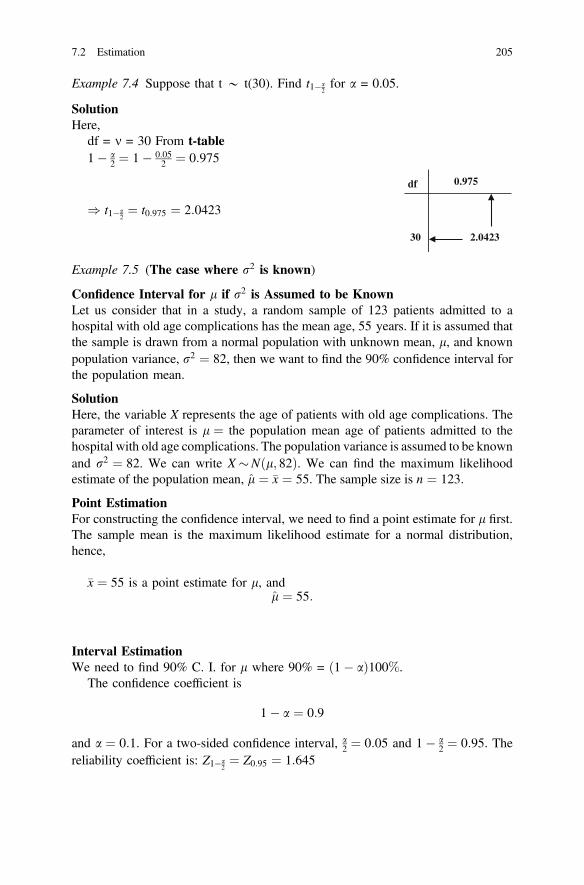
Example 7.4 Suppose that t * t(30). Find t1�a2for a = 0.05.
SolutionHere,
df = m = 30 From t-table1� a
2 ¼ 1� 0:052 ¼ 0:975
) t1�a2¼ t0:975 ¼ 2:0423
df 0.975
30 2.0423
Example 7.5 (The case where r2 is known)
Confidence Interval for l if r2 is Assumed to be KnownLet us consider that in a study, a random sample of 123 patients admitted to ahospital with old age complications has the mean age, 55 years. If it is assumed thatthe sample is drawn from a normal population with unknown mean, l, and knownpopulation variance, r2 ¼ 82, then we want to find the 90% confidence interval forthe population mean.
SolutionHere, the variable X represents the age of patients with old age complications. Theparameter of interest is l ¼ the population mean age of patients admitted to thehospital with old age complications. The population variance is assumed to be knownand r2 ¼ 82. We can write X�Nðl; 82Þ. We can find the maximum likelihoodestimate of the population mean, l ¼ �x ¼ 55. The sample size is n ¼ 123.
Point EstimationFor constructing the confidence interval, we need to find a point estimate for l first.The sample mean is the maximum likelihood estimate for a normal distribution,hence,
�x ¼ 55 is a point estimate for l, andl ¼ 55:
Interval EstimationWe need to find 90% C. I. for l where 90% = 1� að Þ100%.
The confidence coefficient is
1� a ¼ 0:9
and a ¼ 0:1. For a two-sided confidence interval, a2 ¼ 0:05 and 1� a
2 ¼ 0:95. Thereliability coefficient is: Z1�a
2¼ Z0:95 ¼ 1:645
7.2 Estimation 205

The 90% confidence interval for l is
�x� Z1�a2
rffiffiffin
p ;�xþ Z1�a2
rffiffiffin
p� �
:
For the given data, we obtain
55� 1:645ð Þ 9:055ffiffiffiffiffiffiffiffi123
p ; 55þ 1:645ð Þ 9:055ffiffiffiffiffiffiffiffi123
p� �
and the confidence interval for the population mean age of elderly patients with oldage complications is
53:6569; 56:3431ð Þ:
We may interpret this confidence interval in following way: if the samples of thesame size were drawn repeatedly a very large number of times from the samepopulation then in 90% of the times the true value of the population mean would beincluded in the intervals. For this example even if the distribution were not normal,we might have used the same interval because the sample size is large enough forthe application of the central limit theorem.
Example 7.6 Confidence Interval for l if r2 is UnknownLet us consider a hypothetical study on the height of women in their adulthood.
A sample of 24 women is drawn from a normal distribution with population mean land variance r2. The sample mean and variance of height of the selected women are151 cm and 18.65 cm2 respectively. Using given data, we want to construct a 99%confidence interval for the mean height of the adult women in the population fromwhich the sample was drawn randomly.
SolutionLet us summarize the information provided in this example.
The random variable X represents the height of women in their adulthood.The population mean l is unknown. The population variance is r2. The variable
X is distributed as X� Nðl; r2Þ.The sample size is 24. The sample mean and standard deviations are �x ¼ 151
and s ¼ 4:32.
(a) Point Estimation
We need to find a point estimate for l.It may be noted that �x ¼ 151 is a point estimate for l.We obtain l ¼ 151 cm.
206 7 Estimation

(b) Interval Estimation
We need to find 99% C. I. for l, where 99% = 1� að Þ100% and as1� a ¼ 0:99, it can be shown that a ¼ 0:01. For a two-sided interval, we definea2 ¼ 0:005 and 1 � a
2 ¼ 0:995. The sample size is n = 24.
The reliability coefficient is tm;1�a2¼ t23;0:995 ¼ 2:807
df 0.995
23 2.807
From t-table99% confidence interval for l is:The confidence interval for the population mean when the population variance is
unknown can be constructed from the following:
�x� t1�a=2 � s=ffiffiffin
p
where for 99% confidence interval, the lower and upper limits are
l ¼ �x� t1�a=2 � s=ffiffiffin
p
¼ 151� 2:807� 4:32=ffiffiffiffiffi24
p
¼ 151� 2:4753
¼ 148:5247;
and
u ¼ �xþ t1�a=2 � s=ffiffiffin
p
¼ 151þ 2:807� 4:32=ffiffiffiffiffi24
p
¼ 151þ 2:4753
¼ 153:4753:
This can be expressed more precisely as (148.5247,153.4753).If the random samples of size 24 were drawn very large number of times from
the same population then out of all intervals constructed for each sample, 99% ofthe times the population mean would be contained in the intervals. It may be notedhere that for large sample size, the test statistic T would tend to standard normalvariate, Z, asymptotically.
7.2 Estimation 207

7.2.4 Estimation of the Difference Between Two PopulationMeans (l1 − l2)
Suppose that we have two populations such that the first population is characterizedwith mean l1 and variance r21 and the second population with mean l2 and variancer22. We are interested in comparing l1 and l2, or equivalently, making inferencesabout the difference between the means (l1 − l2). We select independently arandom sample of size n1 from the first population and another random sample ofsize n2 from the second population. Let �X1 and S21 be the sample mean and thesample variance of the first sample and �X2 and S22 be the sample mean and thesample variance of the second sample. The sampling distribution of �X1 � �X2 is usedto make inferences about l1 − l2.
The sampling distribution of the difference between two sample means has beendiscussed and the following results are summarized about the sampling distributionof the difference between two sample means:
1. Mean of �X1 � �X2 is l�X1��X2¼ l1 � l2
2. Variance of �X1 � �X2 is r2�X1��X2¼ r21
n1þ r22
n2
3. Standard error of �X1 � �X2 is r�X1��X2¼
ffiffiffiffiffiffiffiffiffiffiffiffiffiffir21n1
þ r22n2
q4. If the two random samples were selected from normal distributions (or
non-normal distributions with large sample sizes) with known variances r21 andr22, then the difference between the sample means ð�X1 � �X2Þ has a normaldistribution with mean ðl1 � l2Þ and variance ððr21=n1Þþ ðr22=n2ÞÞ, that is
�X1 � �X2 �N l1 � l2;r21n1
þ r22n2
� �
and we can show that
Z ¼ ð�X1 � �X2Þ � ðl1 � l2Þffiffiffiffiffiffiffiffiffiffiffiffiffiffir21n1
þ r22n2
q �N 0; 1ð Þ:
(i) Point Estimation of l1 − l2
It can be shown that �X1 � �X2 is a point estimator for l1 − l2.
(ii) Interval Estimation (Confidence Interval) of l1 − l2
We will consider two cases.
A. First Case: r21 and r22 are known
208 7 Estimation

If r21 and r22 are known, we use the following pivotal quantity to find an intervalestimate for l1 − l2.
Z ¼ ð�X1 � �X2Þ � ðl1 � l2Þffiffiffiffiffiffiffiffiffiffiffiffiffiffir21n1
þ r22n2
qA (1 − a)100% confidence interval for l1 − l2 is obtained from the following
probability statement:
Pðza=2\Z\z1�a=2Þ ¼ 1� a:
and it can be shown that
P za=2\Z ¼ ð�X1 � �X2Þ � ðl1 � l2Þffiffiffiffiffiffiffiffiffiffiffiffiffiffir21n1
þ r22n2
q \z1�a=2
0B@1CA ¼ 1� a
¼ P za=2 �ffiffiffiffiffiffiffiffiffiffiffiffiffiffiffiffiffir21n1
þ r22n2
s\ð�X1 � �X2Þ � ðl1 � l2Þ\z1�a=2 �
ffiffiffiffiffiffiffiffiffiffiffiffiffiffiffiffiffir21n1
þ r22n2
s0@ 1A ¼ 1� a
¼ P
�ð�X1 � �X2Þþ za=2 �ffiffiffiffiffiffiffiffiffiffiffiffiffiffiffiffiffir21n1
þ r22n2
s\� ðl1 � l2Þ\� ð�X1 � �X2Þ
þ z1�a=2 �ffiffiffiffiffiffiffiffiffiffiffiffiffiffiffiffiffir21n1
þ r22n2
s0BBBBB@
1CCCCCA ¼ 1� a
¼ P
ð�X1 � �X2Þ � z1�a=2 �ffiffiffiffiffiffiffiffiffiffiffiffiffiffiffiffiffir21n1
þ r22n2
s\ðl1 � l2Þ\ð�X1 � �X2Þ
�za=2 �ffiffiffiffiffiffiffiffiffiffiffiffiffiffiffiffiffir21n1
þ r22n2
s2666664
3777775 ¼ 1� a:
The above interval for the difference between two population means is the1� að Þ 100% confidence interval if population variances are assumed to be known.Using the known relationship Za=2 ¼ �Z1�a=2, the interval can be expressed as
P ð�X1 � �X2Þ � z1�a=2 �ffiffiffiffiffiffiffiffiffiffiffiffiffiffiffiffiffir21n1
þ r22n2
s\ðl1 � l2Þ\ð�X1 � �X2Þþ z1�a=2 �
ffiffiffiffiffiffiffiffiffiffiffiffiffiffiffiffiffir21n1
þ r22n2
s24 35¼ 1� a
7.2 Estimation 209
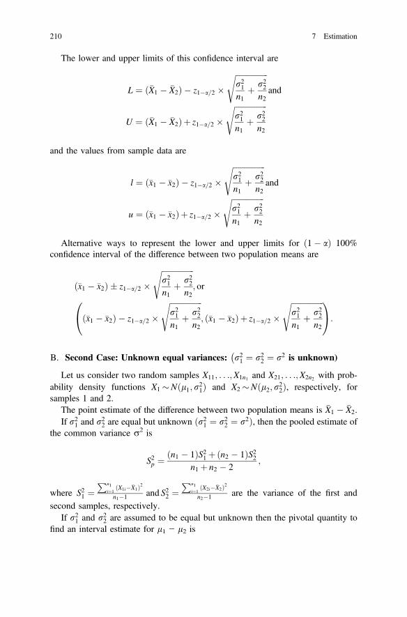
The lower and upper limits of this confidence interval are
L ¼ ð�X1 � �X2Þ � z1�a=2 �ffiffiffiffiffiffiffiffiffiffiffiffiffiffiffiffiffir21n1
þ r22n2
sand
U ¼ ð�X1 � �X2Þþ z1�a=2 �ffiffiffiffiffiffiffiffiffiffiffiffiffiffiffiffiffir21n1
þ r22n2
s
and the values from sample data are
l ¼ ð�x1 � �x2Þ � z1�a=2 �ffiffiffiffiffiffiffiffiffiffiffiffiffiffiffiffiffir21n1
þ r22n2
sand
u ¼ ð�x1 � �x2Þþ z1�a=2 �ffiffiffiffiffiffiffiffiffiffiffiffiffiffiffiffiffir21n1
þ r22n2
s
Alternative ways to represent the lower and upper limits for 1� að Þ 100%confidence interval of the difference between two population means are
ð�x1 � �x2Þ � z1�a=2 �ffiffiffiffiffiffiffiffiffiffiffiffiffiffiffiffiffir21n1
þ r22n2
s; or
ð�x1 � �x2Þ � z1�a=2 �ffiffiffiffiffiffiffiffiffiffiffiffiffiffiffiffiffir21n1
þ r22n2
s; ð�x1 � �x2Þþ z1�a=2 �
ffiffiffiffiffiffiffiffiffiffiffiffiffiffiffiffiffir21n1
þ r22n2
s0@ 1A:
B. Second Case: Unknown equal variances: r21 ¼ r22 ¼ r2�
is unknown)
Let us consider two random samples X11; . . .;X1n1 and X21; . . .;X2n2 with prob-ability density functions X1 �Nðl1; r21Þ and X2 �Nðl2; r22Þ, respectively, forsamples 1 and 2.
The point estimate of the difference between two population means is �X1 � �X2.If r21 and r22 are equal but unknown ðr21 ¼ r22 ¼ r2Þ, then the pooled estimate of
the common variance r2 is
S2p ¼ðn1 � 1ÞS21 þðn2 � 1ÞS22
n1 þ n2 � 2;
where S21 ¼Pn1
i¼1X1i��X1ð Þ2
n1�1 and S22 ¼Pn1
i¼1X2i��X2ð Þ2
n2�1 are the variance of the first andsecond samples, respectively.
If r21 and r22 are assumed to be equal but unknown then the pivotal quantity tofind an interval estimate for l1 − l2 is
210 7 Estimation

T ¼ ð�X1 � �X2Þ � ðl1 � l2ÞffiffiffiffiffiffiffiffiffiffiffiffiffiffiffiffiffiffiffiffiffiffiffiffiS2p
1n1þ 1
n2
� r ;
where T � tn1 þ n2�2.A (1 − a)100% confidence interval for l1 − l2 can be obtained by using the
pivotal quantity as shown below
Pðtðn1 þ n2�2Þ;a=2\T\tðn1 þ n2�2Þ;1�a=2Þ ¼ 1� a:
and it can also be shown that
Pðtðn1 þ n2�2Þ;a=2\T ¼ ð�X1 � �X2Þ � ðl1 � l2ÞffiffiffiffiffiffiffiffiffiffiffiffiffiffiffiffiffiffiffiffiffiffiffiffiS2p
1n1þ 1
n2
� r \tðn1 þ n2�2Þ;1�a=2Þ ¼ 1� a
¼ Pðtðn1 þ n2�2Þ;a=2 �ffiffiffiffiffiffiffiffiffiffiffiffiffiffiffiffiffiffiffiffiffiffiffiffiffiffiffiS2p
1n1
þ 1n2
� �s\ð�X1 � �X2Þ � ðl1 � l2Þ
\tðn1 þ n2�2Þ;1�a=2 �ffiffiffiffiffiffiffiffiffiffiffiffiffiffiffiffiffiffiffiffiffiffiffiffiffiffiffiS2p
1n1
þ 1n2
� �s¼ 1� a
¼ Pð�ð�X1 � �X2Þþ tðn1 þ n2�2Þ;a=2 �ffiffiffiffiffiffiffiffiffiffiffiffiffiffiffiffiffiffiffiffiffiffiffiffiffiffiffiS2p
1n1
þ 1n2
� �s\� ðl1 � l2Þ
\� ð�X1 � �X2Þþ tðn1 þ n2�2Þ;1�a=2 �ffiffiffiffiffiffiffiffiffiffiffiffiffiffiffiffiffiffiffiffiffiffiffiffiffiffiffiS2p
1n1
þ 1n2
� �s¼ 1� a
¼ P
ð�X1 � �X2Þ � tðn1 þ n2�2Þ;1�a=2 �ffiffiffiffiffiffiffiffiffiffiffiffiffiffiffiffiffiffiffiffiffiffiffiffiffiffiffiS2p
1n1
þ 1n2
� �s\ðl1 � l2Þ
\ð�X1 � �X2Þ � tðn1 þ n2�2Þ;a=2 �ffiffiffiffiffiffiffiffiffiffiffiffiffiffiffiffiffiffiffiffiffiffiffiffiffiffiffiS2p
1n1
þ 1n2
� �s2666664
3777775 ¼ 1� a:
The above interval for the difference between two population means is the 1� að Þ100% confidence interval if population variances are assumed to be unknown andequal. Using the known relationship tðn1 þ n2�2Þ;a=2 ¼ �tðn1 þ n2�2Þ;1�a=2, the intervalcan be expressed as
P
ð�X1 � �X2Þ � tðn1 þ n2�2Þ;1�a=2 �ffiffiffiffiffiffiffiffiffiffiffiffiffiffiffiffiffiffiffiffiffiffiffiffiffiffiffiS2p
1n1
þ 1n2
� �s
\ðl1 � l2Þ\ð�X1 � �X2Þ � tðn1 þ n2�2Þ;a=2 �ffiffiffiffiffiffiffiffiffiffiffiffiffiffiffiffiffiffiffiffiffiffiffiffiffiffiffiS2p
1n1
þ 1n2
� �s2666664
3777775 ¼ 1� a:
7.2 Estimation 211

The lower and upper limits of this confidence interval are
L ¼ ð�X1 � �X2Þ � tðn1 þ n2�2Þ;1�a=2 �ffiffiffiffiffiffiffiffiffiffiffiffiffiffiffiffiffiffiffiffiffiffiffiffiffiffiffiS2p
1n1
þ 1n2
� �s; and
U ¼ ð�X1 � �X2Þþ tðn1 þ n2�2Þ;1�a=2 �ffiffiffiffiffiffiffiffiffiffiffiffiffiffiffiffiffiffiffiffiffiffiffiffiffiffiffiS2p
1n1
þ 1n2
� �s:
The lower and upper bounds from sample data can be shown as
l ¼ ð�x1 � �x2Þ � tðn1 þ n2�2Þ;1�a=2 �ffiffiffiffiffiffiffiffiffiffiffiffiffiffiffiffiffiffiffiffiffiffiffiffiffiffiffis2p
1n1
þ 1n2
� �s; and
u ¼ ð�x1 � �x2Þþ tðn1 þ n2�2Þ;1�a=2 �ffiffiffiffiffiffiffiffiffiffiffiffiffiffiffiffiffiffiffiffiffiffiffiffiffiffiffis2p
1n1
þ 1n2
� �s;
where s2p ¼ ðn1�1Þs21 þðn2�1Þs22n1 þ n2�2 ; s21 ¼
Pn1i¼1
x1i��x1ð Þ2n1�1 and s22 ¼
Pn1i¼1
x2i��x2ð Þ2n2�1 .
The 1� að Þ100% lower and upper limits of confidence interval, using sampledata for difference between two population means if the population variances areunknown but assumed to be equal, are shown alternatively as follows:
ð�x1 � �x2Þ � tðn1 þ n2�2Þ;1�a=2 �ffiffiffiffiffiffiffiffiffiffiffiffiffiffiffiffiffiffiffiffiffiffiffiffiffiffiffis2p
1n1
þ 1n2
� �s; or
ð�x1 � �x2Þ � tðn1 þ n2�2Þ;1�a=2 �ffiffiffiffiffiffiffiffiffiffiffiffiffiffiffiffiffiffiffiffiffiffiffiffiffiffiffis2p
1n1
þ 1n2
� �s; ð�x1 � �x2Þ
þ tðn1 þ n2�2Þ;1�a=2 �ffiffiffiffiffiffiffiffiffiffiffiffiffiffiffiffiffiffiffiffiffiffiffiffiffiffiffis2p
1n1
þ 1n2
� �s0BBBBB@
1CCCCCA:
Example 7.7 (Case 1: r21 and r22 are known)Let us consider an experiment for comparing duration of stay of patients in
intensive care unit of a hospital with complication types A and B. Two randomsamples are drawn for types A and B with sample sizes 100 and 70, respectively.Both the random samples are drawn from normally distributed populations withmean and variance lA and r2A for type A and lB and r2B for type B. The meanduration of stay with complication type A is 40 h and with complication type B is50 h. If the population variances for mean duration of stay with complication typesA and B are known to be 15 and 20, respectively, then the interval estimation of thedifference in the population means of duration of stay with complication types Aand B is to be determined. The experimenter wants to find the 95% confidenceinterval for lA − lB.
212 7 Estimation

SolutionLet us summarize the information provided in this example in the following table.
Surgery Type (A) Type (B)
Sample size nA = 100 nB = 70
Sample mean �xA ¼ 40 �xB ¼ 50
Population variance r2A ¼ 15 r2B ¼ 20
A point estimate for lA � lB is
ð�xA � �xBÞ ¼ 40� 50 ¼ �10:
To find a 95% confidence interval for lA � lB, we can define
95% ¼ ð1� aÞ100%
which implies that 0. 95 = (1 − a), a = 0.05 and a/2 = 0.025.The reliability coefficient is z1�a=2 ¼ z0:975 ¼ 1:96.A 95% C.I. for lA � lB is defined as
ð�xA � �xBÞ � Z1�a2
ffiffiffiffiffiffiffiffiffiffiffiffiffiffiffiffiffir2AnA
þ r2BnB
s:
The lower and upper limits can be computed as follows:
�10� Z0:975
ffiffiffiffiffiffiffiffiffiffiffiffiffiffiffiffiffiffiffi15100
þ 2070
rwhich provides
l ¼ �10� 0:8540 ¼ �10:8540
and
u ¼ �10þ 0:8540 ¼ �9:1460:
The above 95% confidence interval of the difference between two means canalso be shown as
�10:8540\lA � lB\� 9:1460:
This confidence interval can be interpreted as: if the samples were drawn frompopulations A and B with sizes nA and nB, respectively, very large number of timesthen the true difference in the population means would be included in the intervalsin 95% of times. There is a link between confidence interval and hypothesis testing
7.2 Estimation 213

because in both the cases we use the statistic known as pivotal quantity in con-structing the confidence interval and test statistic in case of testing a null hypothesis.For instance, since the confidence interval does not include zero, we may concludethat the sample data do not provide evidence in favor of equality of two populationmeans and it may be said that the population means are not equal lA � lBð 6¼ 0 orequivalently, lA 6¼ lBÞ. This will be discussed in more details in Chap. 8.
Example 7.8 (Case II: r21 ¼ r22 unknown)In the previous example, population variances for populations A and B are
assumed to be known. In reality, the population variances are generally not known.Now let us consider a study where samples are drawn from normal populations onthe variables X1= time taken for remission of body temperature from high fever tonormalcy with medication type A and X2= time taken for remission of body tem-perature from high fever to normalcy with medication type B which are assumed tobe distributed as follows
XA �NðlA; r2AÞandXB �NðlB; r2BÞ:
The parameters are unknown. The sample data from populations A and B ontime taken for remission of body temperature from high fever (in hours) are dis-played below
Type A: 55, 70, 35, 48, 71, 40Type B: 30, 35, 52, 64, 25, 45
The experimenter wants to find the 95% confidence interval of the differencebetween mean times of remission of body temperature from high to normal usingmedication types A and B. Let us assume that the population variances are equal,i.e., r2A¼r2B ¼ r2.
SolutionFirst we calculate the mean and the variances of the two samples, and we get
Surgery Type (A) Type (B)
Sample size nA = 6 nB = 6
Sample mean �xA ¼ 53:17 �xB ¼ 41:83
Sample variance S2A ¼ 226:97 S2B ¼ 214:97
(1) A point estimate for lA � lB is
�xA � �xB ¼ 53:17� 41:83 ¼ 11:34:
(2) To find the 95% confidence interval for lA � lB, we need to state thefollowing:
214 7 Estimation
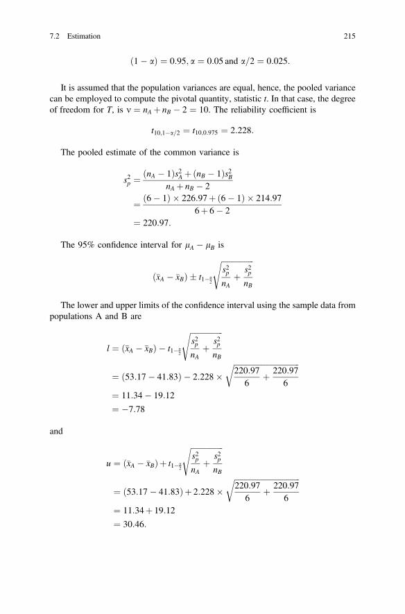
ð1� aÞ ¼ 0:95; a ¼ 0:05 and a=2 ¼ 0:025:
It is assumed that the population variances are equal, hence, the pooled variancecan be employed to compute the pivotal quantity, statistic t. In that case, the degreeof freedom for T, is m ¼ nA þ nB � 2 ¼ 10. The reliability coefficient is
t10;1�a=2 ¼ t10;0:975 ¼ 2:228:
The pooled estimate of the common variance is
s2p ¼ðnA � 1Þs2A þðnB � 1Þs2B
nA þ nB � 2
¼ ð6� 1Þ � 226:97þð6� 1Þ � 214:976þ 6� 2
¼ 220:97:
The 95% confidence interval for lA � lB is
ð�xA � �xBÞ � t1�a2
ffiffiffiffiffiffiffiffiffiffiffiffiffiffiffiffiffis2pnA
þ s2pnB
s
The lower and upper limits of the confidence interval using the sample data frompopulations A and B are
l ¼ ð�xA � �xBÞ � t1�a2
ffiffiffiffiffiffiffiffiffiffiffiffiffiffiffiffiffis2pnA
þ s2pnB
s
¼ ð53:17� 41:83Þ � 2:228�ffiffiffiffiffiffiffiffiffiffiffiffiffiffiffiffiffiffiffiffiffiffiffiffiffiffiffiffiffiffiffiffiffiffi220:97
6þ 220:97
6
r¼ 11:34� 19:12
¼ �7:78
and
u ¼ ð�xA � �xBÞþ t1�a2
ffiffiffiffiffiffiffiffiffiffiffiffiffiffiffiffiffis2pnA
þ s2pnB
s
¼ ð53:17� 41:83Þþ 2:228�ffiffiffiffiffiffiffiffiffiffiffiffiffiffiffiffiffiffiffiffiffiffiffiffiffiffiffiffiffiffiffiffiffiffi220:97
6þ 220:97
6
r¼ 11:34þ 19:12
¼ 30:46:
7.2 Estimation 215

This can be shown as
�7:78\lA � lB\30:46:
95% of the times, the confidence interval for difference between the true pop-ulation means would include the true difference between the population means outof all the intervals calculated for each of the samples of same size drawn repeatedlyvery large number of times. Since the confidence interval includes zero, we con-clude that the two population means may be equal (lA − lB= 0, equivalently,lA= lB). Therefore, we may conclude that the mean time required for remission ofbody temperature is the same for the two types.
7.2.5 Estimation of a Population Proportion (P)
If we recall from Chap. 6, the random variable X = number of elements or subjectswith a specified characteristic A, N = total number of elements in the populationand n = total number of elements in the sample. The probability of a randomlyselected subject or element has characteristic A is denoted by p which is essentiallythe proportion of elements or subjects with characteristic A in the population. Wedefined Xi ¼ 1, if the ith Bernoulli trial results in selecting an element or subjectwith characteristic A, Xi ¼ 0, if the selected element does not have characteristicA. After conducting the trial on n elements of the sample independently, we haveX ¼Pn
i¼1 Xi = the number of elements or subjects selected with characteristic A.The joint distribution of n Bernoulli variables X1; . . .;Xnð Þ, if Xi s are inde-
pendently and identically distributed, is
f ðx1; . . .; xn; pÞ ¼Yni¼1
f ðxi; pÞ ¼Yni¼1
pxið1� pÞð1�xiÞ ¼ pxð1� pÞn�x
and the distribution of X ¼ x, where X is the sum of n Bernoulli variables, is
f ðx; n; pÞ ¼ n
x
!pxð1� pÞn�x
where the number of mutually exclusive events isn
x
!. This probability function
is similar to the likelihood function of the Bernoulli distribution for X1; . . .;Xn butthe difference between the Bernoulli and binomial trials is that in Bernoulli trial, weare interested in the sequence of outcomes for elements in a Bernoulli trial but intotal number of successes, X, out of n in a binomial distribution where n is fixed.Then the likelihood function of p for known value of n is
216 7 Estimation
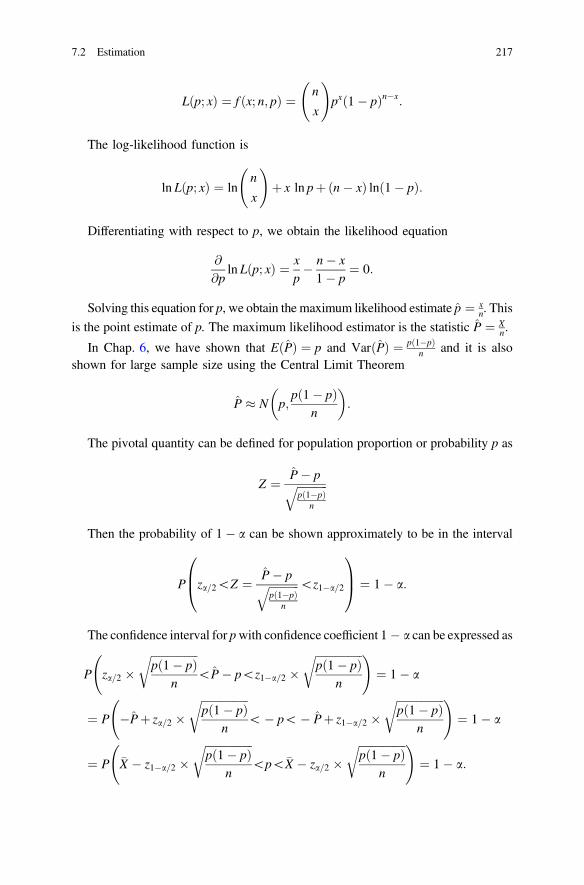
Lðp; xÞ ¼ f ðx; n; pÞ ¼ n
x
!pxð1� pÞn�x:
The log-likelihood function is
ln Lðp; xÞ ¼ lnn
x
!þ x ln pþðn� xÞ lnð1� pÞ:
Differentiating with respect to p, we obtain the likelihood equation
@
@pln Lðp; xÞ ¼ x
p� n� x1� p
¼ 0:
Solving this equation for p, we obtain the maximum likelihood estimate p ¼ xn. This
is the point estimate of p. The maximum likelihood estimator is the statistic P ¼ Xn.
In Chap. 6, we have shown that EðPÞ ¼ p and VarðPÞ ¼ pð1�pÞn and it is also
shown for large sample size using the Central Limit Theorem
P N p;pð1� pÞ
n
� �:
The pivotal quantity can be defined for population proportion or probability p as
Z ¼ P� pffiffiffiffiffiffiffiffiffiffiffipð1�pÞ
n
qThen the probability of 1� a can be shown approximately to be in the interval
P za=2\Z ¼ P� pffiffiffiffiffiffiffiffiffiffiffipð1�pÞ
n
q \z1�a=2
0B@1CA ¼ 1� a:
The confidence interval for pwith confidence coefficient 1� a can be expressed as
P za=2 �ffiffiffiffiffiffiffiffiffiffiffiffiffiffiffiffiffipð1� pÞ
n
r\P� p\z1�a=2 �
ffiffiffiffiffiffiffiffiffiffiffiffiffiffiffiffiffipð1� pÞ
n
r !¼ 1� a
¼ P �Pþ za=2 �ffiffiffiffiffiffiffiffiffiffiffiffiffiffiffiffiffipð1� pÞ
n
r\� p\� Pþ z1�a=2 �
ffiffiffiffiffiffiffiffiffiffiffiffiffiffiffiffiffipð1� pÞ
n
r !¼ 1� a
¼ P �X � z1�a=2 �ffiffiffiffiffiffiffiffiffiffiffiffiffiffiffiffiffipð1� pÞ
n
r\p\�X � za=2 �
ffiffiffiffiffiffiffiffiffiffiffiffiffiffiffiffiffipð1� pÞ
n
r !¼ 1� a:
7.2 Estimation 217

The above interval is the 1� að Þ 100% confidence interval for populationproportion p for large sample size. Using the relationship Za=2 ¼ �Z1�a=2 forstandard normal distribution, the confidence interval can be expressed as
P P� z1�a=2 �ffiffiffiffiffiffiffiffiffiffiffiffiffiffiffiffiffipð1� pÞ
n
r\p\Pþ z1�a=2 �
ffiffiffiffiffiffiffiffiffiffiffiffiffiffiffiffiffipð1� pÞ
n
r !¼ 1� a:
The lower and upper limits or end points of this confidence interval are
L ¼ P� z1�a=2 �ffiffiffiffiffiffiffiffiffiffiffiffiffiffiffiffiffipð1� pÞ
n
rand
U ¼ Pþ z1�a=2 �ffiffiffiffiffiffiffiffiffiffiffiffiffiffiffiffiffipð1� pÞ
n
r:
Using the sample data, the lower and upper limits of the confidence interval are
l ¼ p� z1�a=2 �ffiffiffiffiffiffiffiffiffiffiffiffiffiffiffiffiffipð1� pÞ
n
rand
u ¼ pþ z1�a=2 �ffiffiffiffiffiffiffiffiffiffiffiffiffiffiffiffiffipð1� pÞ
n
r:
Alternative MethodsThe method of constructing confidence interval of a proportion discussed above isbased on the asymptotic normality of the sample proportion. This is the mostpopular way to present confidence interval for proportion or binomial parameterp. However, several studies such as studies by Agresti and Coull (1998) and Brownet al. (2001) showed that this method, known as the Wald confidence interval for p,first proposed by Laplace (1812) and may be considered as one of the oldestconfidence intervals proposed for a parameter, may provide very erratic behavior ofthe coverage probability even for a large n, where the value of large n may be quitearbitrary and vague in case of sample proportion. The Wald confidence interval forp based on asymptotic normality may produce small coverage probability. It is alsoknown that the coverage probability is poor for p near 0 or 1. In many cases evenwith the assumption that n�minðp; 1� pÞ should be at least 5 (some prefer 10)may produce poor coverage for p near 0 or 1. Brown et al. (2001) showed that evenwhen this condition is satisfied, there is no guarantee that the coverage probabilityis close to confidence level. As an alternative, Clopper and Pearson (1934) exactmethod is suggested for p where a hypothesized value for p, say p0, is used tocompute lower and upper end points as shown below
218 7 Estimation
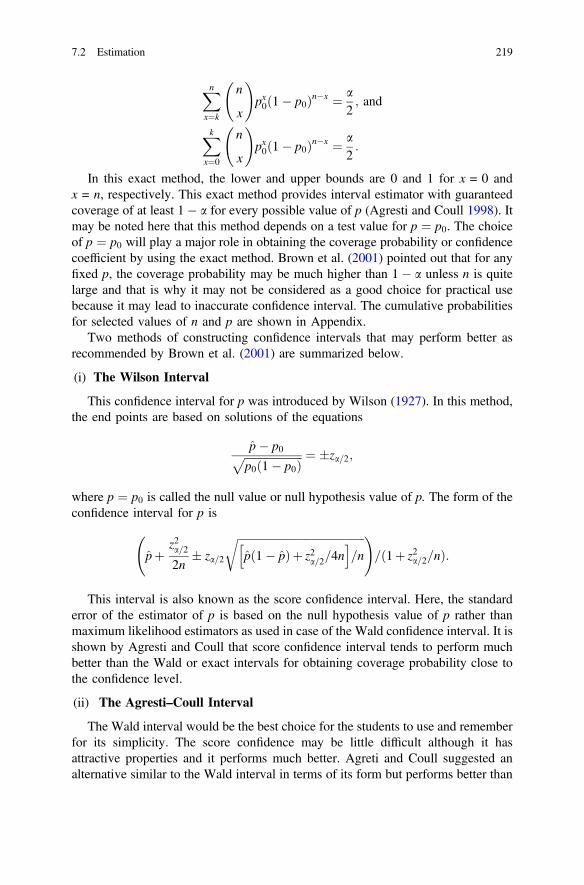
Xnx¼k
n
x
!px0ð1� p0Þn�x ¼ a
2; and
Xkx¼0
n
x
!px0ð1� p0Þn�x ¼ a
2:
In this exact method, the lower and upper bounds are 0 and 1 for x = 0 andx = n, respectively. This exact method provides interval estimator with guaranteedcoverage of at least 1� a for every possible value of p (Agresti and Coull 1998). Itmay be noted here that this method depends on a test value for p ¼ p0. The choiceof p ¼ p0 will play a major role in obtaining the coverage probability or confidencecoefficient by using the exact method. Brown et al. (2001) pointed out that for anyfixed p, the coverage probability may be much higher than 1� a unless n is quitelarge and that is why it may not be considered as a good choice for practical usebecause it may lead to inaccurate confidence interval. The cumulative probabilitiesfor selected values of n and p are shown in Appendix.
Two methods of constructing confidence intervals that may perform better asrecommended by Brown et al. (2001) are summarized below.
(i) The Wilson Interval
This confidence interval for p was introduced by Wilson (1927). In this method,the end points are based on solutions of the equations
p� p0ffiffiffiffiffiffiffiffiffiffiffiffiffiffiffiffiffiffiffiffiffip0ð1� p0Þ
p ¼ �za=2;
where p ¼ p0 is called the null value or null hypothesis value of p. The form of theconfidence interval for p is
pþz2a=22n
� za=2
ffiffiffiffiffiffiffiffiffiffiffiffiffiffiffiffiffiffiffiffiffiffiffiffiffiffiffiffiffiffiffiffiffiffiffiffiffiffiffiffiffiffiffiffiffiffipð1� pÞþ z2a=2=4nh i
=n
r !=ð1þ z2a=2=nÞ:
This interval is also known as the score confidence interval. Here, the standarderror of the estimator of p is based on the null hypothesis value of p rather thanmaximum likelihood estimators as used in case of the Wald confidence interval. It isshown by Agresti and Coull that score confidence interval tends to perform muchbetter than the Wald or exact intervals for obtaining coverage probability close tothe confidence level.
(ii) The Agresti–Coull Interval
The Wald interval would be the best choice for the students to use and rememberfor its simplicity. The score confidence may be little difficult although it hasattractive properties and it performs much better. Agreti and Coull suggested analternative similar to the Wald interval in terms of its form but performs better than
7.2 Estimation 219

the Wald interval and they named it as the “add two successes and two failures”adjusted Wald interval. In this method, instead of p ¼ X
n, it is suggested that ~p ¼ ~X~n ;
where ~X ¼ X þ z2a=2=2 and ~n ¼ nþ z2a=2. For 95% confidence interval for p,
a ¼ 0:05 so that za=2 ¼ 1:96 2 and z2a=2 ¼ 1:962 4, the Agresti–Coull point
estimator is
~p ¼~X~n¼ Xþ 2
nþ 4:
The Agresti–Coull confidence interval with confidence level 1� a is
~p� za=2~pð1� ~pÞffiffiffi
~np ;
where the lower and upper end points are
l ¼ ~p� za=2~pð1� ~pÞffiffiffi
~np ; and
u ¼ ~pþ za=2~pð1� ~pÞffiffiffi
~np :
Both the Wilson interval and Agresti–Coull interval are centered on the samevalue, ~p, and Agresti–Coull intervals are never shorter than the Wilson intervals(Brown et al. 2001).
Example 7.9 In a study on the diagnosis of acute inflammations of urinary bladderand acute nephritises, a sample of 120 is considered (Czerniak and Zarzycki 2003).Out of 120 in the sample, 50 are found to have acute nephritis of renal pelvis origin.Then we want to find the point estimate and the 95% confidence interval for the trueproportion of acute nephritis of renal pelvis origin.
SolutionThe variable is X = number of subjects having acute nephritis of renal pelvis origin.The sample size is n = 120. The number of subjects with acute nephritis of renalpelvis origin is 50. The sample proportion is
p ¼ xn¼ 50
120¼ 0:4167:
A point estimate for p is p ¼ 0:4167.For constructing the 95% confidence interval for proportion, p, let us defineThe confidence coefficient = 1� a ¼ 0:95; a ¼ 0:05; a=2 ¼ 0:025.The reliability coefficient = z1�a=2 ¼ z0:975 ¼ 1:96.The 95% confidence interval for proportion of acute nephritis of renal pelvis
region is
220 7 Estimation
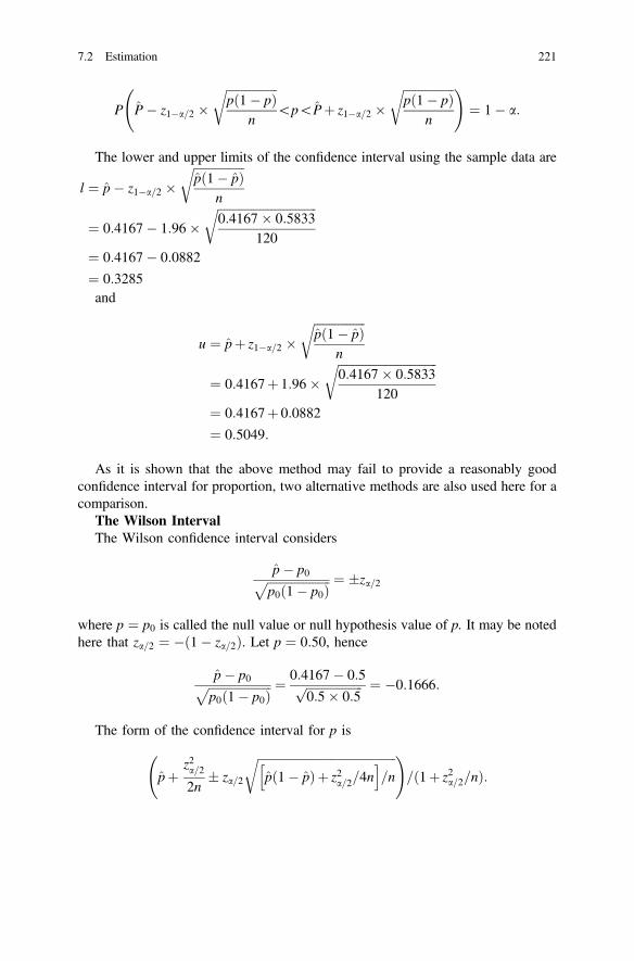
P P� z1�a=2 �ffiffiffiffiffiffiffiffiffiffiffiffiffiffiffiffiffipð1� pÞ
n
r\p\Pþ z1�a=2 �
ffiffiffiffiffiffiffiffiffiffiffiffiffiffiffiffiffipð1� pÞ
n
r !¼ 1� a:
The lower and upper limits of the confidence interval using the sample data are
l ¼ p� z1�a=2 �ffiffiffiffiffiffiffiffiffiffiffiffiffiffiffiffiffipð1� pÞ
n
r¼ 0:4167� 1:96�
ffiffiffiffiffiffiffiffiffiffiffiffiffiffiffiffiffiffiffiffiffiffiffiffiffiffiffiffiffiffiffiffiffi0:4167� 0:5833
120
r¼ 0:4167� 0:0882
¼ 0:3285and
u ¼ pþ z1�a=2 �ffiffiffiffiffiffiffiffiffiffiffiffiffiffiffiffiffipð1� pÞ
n
r¼ 0:4167þ 1:96�
ffiffiffiffiffiffiffiffiffiffiffiffiffiffiffiffiffiffiffiffiffiffiffiffiffiffiffiffiffiffiffiffiffi0:4167� 0:5833
120
r¼ 0:4167þ 0:0882
¼ 0:5049:
As it is shown that the above method may fail to provide a reasonably goodconfidence interval for proportion, two alternative methods are also used here for acomparison.
The Wilson IntervalThe Wilson confidence interval considers
p� p0ffiffiffiffiffiffiffiffiffiffiffiffiffiffiffiffiffiffiffiffiffip0ð1� p0Þ
p ¼ �za=2
where p ¼ p0 is called the null value or null hypothesis value of p. It may be notedhere that za=2 ¼ �ð1� za=2Þ. Let p ¼ 0:50, hence
p� p0ffiffiffiffiffiffiffiffiffiffiffiffiffiffiffiffiffiffiffiffiffip0ð1� p0Þ
p ¼ 0:4167� 0:5ffiffiffiffiffiffiffiffiffiffiffiffiffiffiffiffiffiffiffi0:5� 0:5
p ¼ �0:1666:
The form of the confidence interval for p is
pþz2a=22n
� za=2
ffiffiffiffiffiffiffiffiffiffiffiffiffiffiffiffiffiffiffiffiffiffiffiffiffiffiffiffiffiffiffiffiffiffiffiffiffiffiffiffiffiffiffiffiffiffipð1� pÞþ z2a=2=4nh i
=n
r !=ð1þ z2a=2=nÞ:
7.2 Estimation 221

The lower and upper limits are
l ¼ pþz2a=22n
þ za=2
ffiffiffiffiffiffiffiffiffiffiffiffiffiffiffiffiffiffiffiffiffiffiffiffiffiffiffiffiffiffiffiffiffiffiffiffiffiffiffiffiffiffiffiffiffiffipð1� pÞþ z2a=2=4nh i
=n
r !=ð1þ z2a=2=nÞ
¼0:4167þ ð�0:1666Þ2
2� 120þð�0:1666�ffiffiffiffiffiffiffiffiffiffiffiffiffiffiffiffiffiffiffiffiffiffiffiffiffiffiffiffiffiffiffiffiffiffiffiffiffiffiffiffiffiffiffiffiffiffiffiffiffiffiffiffiffiffiffiffiffiffiffiffiffiffiffiffiffiffiffiffiffiffiffiffiffiffiffiffiffiffiffiffiffiffiffiffiffiffiffiffiffiffiffiffiffiffiffiffi
0:4167� 0:5833þð�0:1666Þ2=ð4� 120Þh i
=120
r0BBB@
1CCCA=½1þð�0:1666Þ2=120�
¼ 0:4092
u ¼ pþz2a=22n
� za=2
ffiffiffiffiffiffiffiffiffiffiffiffiffiffiffiffiffiffiffiffiffiffiffiffiffiffiffiffiffiffiffiffiffiffiffiffiffiffiffiffiffiffiffiffiffiffipð1� pÞþ z2a=2=4nh i
=n
r !=ð1þ z2a=2=nÞ
¼0:4167þ ð�0:1666Þ2
2� 120� ð�0:1666�ffiffiffiffiffiffiffiffiffiffiffiffiffiffiffiffiffiffiffiffiffiffiffiffiffiffiffiffiffiffiffiffiffiffiffiffiffiffiffiffiffiffiffiffiffiffiffiffiffiffiffiffiffiffiffiffiffiffiffiffiffiffiffiffiffiffiffiffiffiffiffiffiffiffiffiffiffiffiffiffiffiffiffiffiffiffiffiffiffiffiffiffiffiffiffiffi
0:4167� 0:5833þð�0:1666Þ2=ð4� 120Þh i
=120
r0BBB@
1CCCA=½1þð�0:1666Þ2=120�
¼ 0:4242:
The Agresti–Coull Interval
Agresti and Coull suggested an alternative similar to the Wald interval shown asthe first example that performs better than the Wald interval and it is called as “addtwo successes and two failures” adjusted Wald interval.
In this method, instead of p ¼ Xn, we use the estimator ~p ¼ ~X
~n ;
where ~X ¼ X þ z21�a=2=2 and ~n ¼ nþ z21�a=2. For 95% confidence interval for p,
a ¼ 0:05 so that z1�a=2 ¼ 1:96 2 and z21�a=2 ¼ 1:962 4, the Agresti–Coull
point estimator is
~p ¼~X~n¼ Xþ 2
nþ 4¼ 50þ 2
120þ 4¼ 0:4194:
The Agresti–Coull confidence interval with confidence level 0.95 is
~p� z0:95 � ~pð1� ~pÞffiffiffi~n
p ;
222 7 Estimation

where the lower and upper end points are
l ¼ ~p� z1�a=2 �~pð1� ~pÞffiffiffi
~np
¼ 0:4194� 2� 0:4194� 0:5806ffiffiffiffiffiffiffiffi124
p
¼ 0:4194� 0:0437
¼ 0:3757;
and
u ¼ ~pþ z1�a=2 �~pð1� ~pÞffiffiffi
~np
¼ 0:4194þ 2� 0:4194� 0:5806ffiffiffiffiffiffiffiffi124
p
¼ 0:4194þ 0:0437
¼ 0:4631:
Both the Wilson interval and Agresti–Coull interval are centered on the samevalue, ~p, but it is seen that the Agresti–Coull interval is larger than the Wilsoninterval.
7.2.6 Estimation of the Difference Between Two PopulationProportions ðp1 � p2Þ
Let us define two independent random samples X11; . . .;X1n1ð Þ and X21; . . .;X2n2ð Þwith sample size n1 and n2, respectively. The random sample 1 is drawn fromX1i �Bernoulliðp1Þ and the second sample from X2i �Bernoulliðp2Þ. Here X1i ¼ 1,if the ith Bernoulli trial (or simply ith element of the random sample 1) results inselecting an element with a specified characteristic A in sample 1; X1i ¼ 0, other-wise and X2i ¼ 1, if the ith Bernoulli trial (or simply ith element of the randomsample 2) results in selecting an element with a specified characteristic A in sample2; X2i ¼ 0, otherwise. Then let us define X1 ¼
Pn1i¼1 X1i and X2 ¼
Pn1i¼1 X2i repre-
senting number of elements with characteristic A in samples 1 and 2, respectively.The probability distributions of X1 ¼
Pn1i¼1 X1i andX2 ¼
Pn1i¼1 X2i are then
X1 �Binomialðp1Þ for random sample and the second sample fromX2 �Binomialðp2Þ.
7.2 Estimation 223
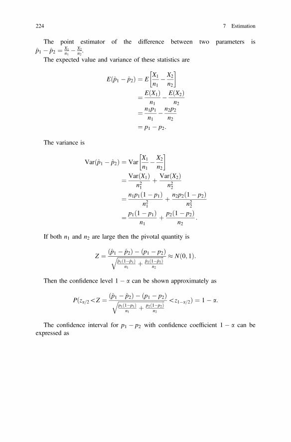
The point estimator of the difference between two parameters isp1 � p2 ¼ X1
n1� X2
n2.
The expected value and variance of these statistics are
Eðp1 � p2Þ ¼ EX1
n1� X2
n2
�¼ EðX1Þ
n1� EðX2Þ
n2
¼ n1p1n1
� n2p2n2
¼ p1 � p2:
The variance is
Varðp1 � p2Þ ¼ VarX1
n1� X2
n2
�¼ VarðX1Þ
n21þ VarðX2Þ
n22
¼ n1p1ð1� p1Þn21
þ n2p2ð1� p2Þn22
¼ p1ð1� p1Þn1
þ p2ð1� p2Þn2
:
If both n1 and n2 are large then the pivotal quantity is
Z ¼ p1 � p2ð Þ � p1 � p2ð Þffiffiffiffiffiffiffiffiffiffiffiffiffiffiffiffiffiffiffiffiffiffiffiffiffiffiffiffiffiffiffiffiffiffip1ð1�p1Þ
n1þ p2ð1�p2Þ
n2
q Nð0; 1Þ:
Then the confidence level 1� a can be shown approximately as
Pðza=2\Z ¼ p1 � p2ð Þ � p1 � p2ð Þffiffiffiffiffiffiffiffiffiffiffiffiffiffiffiffiffiffiffiffiffiffiffiffiffiffiffiffiffiffiffiffiffiffip1ð1�p1Þ
n1þ p2ð1�p2Þ
n2
q \z1�a=2Þ ¼ 1� a:
The confidence interval for p1 � p2 with confidence coefficient 1� a can beexpressed as
224 7 Estimation

P
za=2 �ffiffiffiffiffiffiffiffiffiffiffiffiffiffiffiffiffiffiffiffiffiffiffiffiffiffiffiffiffiffiffiffiffiffiffiffiffiffiffiffiffiffiffiffiffiffiffiffiffip1ð1� p1Þ
n1þ p2ð1� p2Þ
n2
s\ p1 � p2ð Þ � p1 � p2ð Þ
\z1�a=2 �ffiffiffiffiffiffiffiffiffiffiffiffiffiffiffiffiffiffiffiffiffiffiffiffiffiffiffiffiffiffiffiffiffiffiffiffiffiffiffiffiffiffiffiffiffiffiffiffiffip1ð1� p1Þ
n1þ p2ð1� p2Þ
n2
s0BBBBB@
1CCCCCA ¼ 1� a
¼ P
� p1 � p2ð Þþ za=2 �ffiffiffiffiffiffiffiffiffiffiffiffiffiffiffiffiffiffiffiffiffiffiffiffiffiffiffiffiffiffiffiffiffiffiffiffiffiffiffiffiffiffiffiffiffiffiffiffiffip1ð1� p1Þ
n1þ p2ð1� p2Þ
n2
s\� p1 � p2ð Þ
\� p1 � p2ð Þþ z1�a=2 �ffiffiffiffiffiffiffiffiffiffiffiffiffiffiffiffiffiffiffiffiffiffiffiffiffiffiffiffiffiffiffiffiffiffiffiffiffiffiffiffiffiffiffiffiffiffiffiffiffip1ð1� p1Þ
n1þ p2ð1� p2Þ
n2
s0BBBBB@
1CCCCCA ¼ 1� a
¼ P
p1 � p2ð Þ � z1�a=2 �ffiffiffiffiffiffiffiffiffiffiffiffiffiffiffiffiffiffiffiffiffiffiffiffiffiffiffiffiffiffiffiffiffiffiffiffiffiffiffiffiffiffiffiffiffiffiffiffiffip1ð1� p1Þ
n1þ p2ð1� p2Þ
n2
s\ p1 � p2ð Þ
\ p1 � p2ð Þ � za=2 �ffiffiffiffiffiffiffiffiffiffiffiffiffiffiffiffiffiffiffiffiffiffiffiffiffiffiffiffiffiffiffiffiffiffiffiffiffiffiffiffiffiffiffiffiffiffiffiffiffip1ð1� p1Þ
n1þ p2ð1� p2Þ
n2
s0BBBBB@
1CCCCCA ¼ 1� a:
Using the relationship Za=2 ¼ �Z1�a=2 and replacing p1 and p2 by maximumlikelihood estimators in the lower and upper end points, the confidence interval canbe expressed as
P
p1 � p2ð Þ � z1�a=2 �ffiffiffiffiffiffiffiffiffiffiffiffiffiffiffiffiffiffiffiffiffiffiffiffiffiffiffiffiffiffiffiffiffiffiffiffiffiffiffiffiffiffiffiffiffiffiffiffiffip1ð1� p1Þ
n1þ p2ð1� p2Þ
n2
s\ p1 � p2ð Þ\ p1 � p2ð Þ
þ z1�a=2 �ffiffiffiffiffiffiffiffiffiffiffiffiffiffiffiffiffiffiffiffiffiffiffiffiffiffiffiffiffiffiffiffiffiffiffiffiffiffiffiffiffiffiffiffiffiffiffiffiffip1ð1� p1Þ
n1þ p2ð1� p2Þ
n2
s0BBBBB@
1CCCCCA¼ 1� a:
The lower and upper limits or end points of this confidence interval, using theestimates of the proportions, are
l ¼ p1 � p2ð Þ � z1�a=2 �ffiffiffiffiffiffiffiffiffiffiffiffiffiffiffiffiffiffiffiffiffiffiffiffiffiffiffiffiffiffiffiffiffiffiffiffiffiffiffiffiffiffiffiffiffiffiffiffiffip1ð1� p1Þ
n1þ p2ð1� p2Þ
n2
sand
u ¼ p1 � p2ð Þþ z1�a=2 �ffiffiffiffiffiffiffiffiffiffiffiffiffiffiffiffiffiffiffiffiffiffiffiffiffiffiffiffiffiffiffiffiffiffiffiffiffiffiffiffiffiffiffiffiffiffiffiffiffip1ð1� p1Þ
n1þ p2ð1� p2Þ
n2
s:
Example 7.10 A researcher was interested in comparing the proportion of peoplesuffering from breathing problem in two cities, A and B. A random sample of 2500people is taken from city A, and another independent random sample of 2000people is taken from city B. It is found that 110 people in city A and 74 people in
7.2 Estimation 225

city B have been found with breathing problem. The researcher is interested infinding the 90% confidence interval of the difference between the two proportions.
SolutionLet us define the parameters and estimators for the populations A and B:
p1 population proportion of people having breathing problem in city A,p2 population proportion of people having breathing problem in city B,x1 number of people with breathing problem in the sample from city A,x2 number of people with breathing problem in the sample from city B,n1 sample size for city A,n2 sample size for city B,p1 sample proportion of the sample from city A, andp2 sample proportion of the sample from city B.
The point estimates of proportions with breathing problems in cities A and B areshown below:
p1 ¼ x1n1
¼ 1102500
¼ 0:044;
p2 ¼ x2n2
¼ 742000:
¼ 0:037
Point Estimation for p1 − p2:The point estimate for the difference between the two proportions, p1 − p2, is
p1 � p2 ¼ 0:044� 0:037 ¼ 0:007:
The lower and upper limits or end points of this confidence interval, using theestimates of the proportions, are
l ¼ p1 � p2ð Þ � z1�a=2 �ffiffiffiffiffiffiffiffiffiffiffiffiffiffiffiffiffiffiffiffiffiffiffiffiffiffiffiffiffiffiffiffiffiffiffiffiffiffiffiffiffiffiffiffiffiffiffiffiffip1ð1� p1Þ
n1þ p2ð1� p2Þ
n2
s
¼ 0:007� 1:645�ffiffiffiffiffiffiffiffiffiffiffiffiffiffiffiffiffiffiffiffiffiffiffiffiffiffiffiffiffiffiffiffiffiffiffiffiffiffiffiffiffiffiffiffiffiffiffiffiffiffiffiffiffiffiffiffiffiffiffiffiffiffiffi0:044� 0:956
2500þ 0:037� 0:963
2000
r¼ 0:007� 0:0097
¼ �0:0027
226 7 Estimation

and
u ¼ p1 � p2ð Þþ z1�a=2 �ffiffiffiffiffiffiffiffiffiffiffiffiffiffiffiffiffiffiffiffiffiffiffiffiffiffiffiffiffiffiffiffiffiffiffiffiffiffiffiffiffiffiffiffiffiffiffiffiffip1ð1� p1Þ
n1þ p2ð1� p2Þ
n2
s
¼ 0:007þ 1:645�ffiffiffiffiffiffiffiffiffiffiffiffiffiffiffiffiffiffiffiffiffiffiffiffiffiffiffiffiffiffiffiffiffiffiffiffiffiffiffiffiffiffiffiffiffiffiffiffiffiffiffiffiffiffiffiffiffiffiffiffiffiffiffi0:044� 0:956
2500þ 0:037� 0:963
2000
r¼ 0:007þ 0:0097
¼ 0:0167:
The 95% confidence interval for the difference between two proportions forcities A and B is (−0.0027, 0.0167). This includes 0 that indicates the no differencebetween the proportions.
7.3 Summary
In this chapter, the concepts and applications of estimation are discussed. Themethods of point estimation namely the method of maximum likelihood and themethod of moments are introduced in this chapter. The interval estimation is alsohighlighted in this chapter and the construction of confidence intervals are dis-cussed at length. The construction of confidence interval for single populationmean, difference between two population means, single population proportion, anddifference between two population proportions are shown with examples underdifferent underlying assumptions about population as well as about small or largesample sizes. The pivotal quantities under the assumption of known or unknownvariances are also highlighted. In addition to the traditional Wald method, alter-native methods of interval estimation of the population proportion namely the exactmethod, the Wilson method and the Agresti–Coull method are also illustrated withexamples.
Exercises
7:1 Define the following briefly with example:
(i) Parameter,(ii) Statistic,(iii) Estimator,(iv) Estimate.
7:2 Find the estimator of the parameter of the Bernoulli distribution using themethod of moments.
7:3 Write the probability mass function of the geometric distribution and find theestimator of the parameter using method of moments.
7.2 Estimation 227

7:4 Using the method of moments, find the estimator of the parameters of anormal distribution.
7:5
(i) What is the difference between joint density function and likelihoodfunction?
(ii) Write the likelihood function for a Poisson distribution.(iii) Find the likelihood estimators of the parameters of a Poisson
distribution.
7:6 Use the method of moments to estimate the parameter of the followingdistribution:
f ðy; hÞ ¼ 1he�
yh:
7:7
(i) Find the 100ð1� aÞ% confidence interval for the population mean l ifthe variance r2 is known.
(ii) Consider that the time necessary for conducting a surgery is distributedas normal with population mean l and variance r2, where variance isknown. A study is conducted to find the estimate of the populationmean. The sample size is n = 40 and the estimated mean time is �x ¼ 25minutes. The population variance is known to be 15 min2. Find the 99%confidence interval of the population mean time of performing thesurgery. Interpret your result.
7:8
(i) Find the 100ð1� aÞ% confidence interval for the population mean l ifthe variance r2 is known. A sample of size n is drawn from anon-normal population with the population mean l and known variancer2.
(ii) A study is conducted on children under 5 years regarding duration ofbreathing problem (in days) due to environmental problems in a city.The size of the sample is 75. The probability distribution of the variable,duration of breathing problem, is not normal. The population mean is land the variance is known r2 ¼ 3 days2. The estimated mean time is�x ¼ 5 days. Find the 95% confidence interval of the population meanduration of breathing problem among children of under 5 years.Interpret your result.
7:9
(i) Find the 100ð1� aÞ% confidence interval for the population mean l ifthe variance r2 is unknown.
228 7 Estimation
(ii) In a study on blood glucose level among adult population, it is foundthat the mean glucose level and standard deviation are 80 mg/dL and27 mg/dL, respectively. The sample size is 21. Find the 95% confidenceinterval of the population mean glucose level among adult population.Interpret your result.
7:10
(i) Find the 100ð1� aÞ% confidence interval for difference between twopopulation means if r21 and r22 are unknown and assumed to be equal.
(ii) An experiment was conducted to compare time duration of stay in ahospital with two types of complications (A) and (B) and 9 patientswith complication type A and 16 patients with complication type Bwere selected randomly. The average time lengths were 12 days for Aand 7 days for B and sample variances were 8 days2 for A and 5 days2
for B. Assuming equality of variances in the populations, find the 99%confidence interval for the difference in population means of A and B.
7:11
(i) Find the 90% confidence interval for population proportion, p, if p ¼0:4 and n = 100 using the asymptotic normality assumption.
(ii) Use the alternative methods: (a) exact method, (b) Wilson interval and(c) Agresti–Coull interval for constructing confidence interval.
(iii) Compare all these confidence intervals and comment on the suitabilityof confidence intervals for the given data.
7:12 Among the adult males and females, a study is conducted to estimate theproportion of diabetics. The sample sizes are 250 for males and 200 forfemales. It is found from the estimates from the samples that the proportionof diabetics among males is 10% and among females is 7%. Find the 95%confidence interval of the difference between population proportions formales and females.
7:13
(i) What is interval estimation? Define the 100 ð1� aÞ% confidenceinterval and illustrate with a pivotal quantity.
(ii) Find the 100ð1� aÞ% confidence interval for the difference betweentwo population means for two correlated variables.
7:14
(i) Briefly describe the method of estimating parameters by the method ofmaximum likelihood.
(ii) Let X1; . . .;Xn be a random sample from the following population:
f ðx; l; 5Þ ¼ 1ffiffiffiffiffiffi10p
p e�110ðx�lÞ2 , and find the maximum likelihood estimators
of the parameters. If l is the ML estimator of l then find the MLestimator of l2.
7.3 Summary 229

7:15 Consider the following probability mass functions:
f ðx; n; pÞ ¼ n
x
!pxqn�x; x ¼ 0; 1; . . .; n;
Find the estimator of p using the method of moments and the method ofmaximum likelihood.
7:16 Find the 100ð1� aÞ% confidence interval for the difference between twomeans, l1 � l2, if r
21 and r22 are unknown and assumed to be unequal and
sample sizes are small; also indicate what would be the confidence interval ifthe sample sizes are large.
7:17 Consider the following probability mass function:
f ðx; hÞ ¼ e�hhx
x!; x ¼ 0; 1; . . .
(i) Find the estimator of the parameter of the above pmf for a randomsample X1; . . .;Xn using the method of moments.
(ii) Find the estimator of the parameter of the above pmf for a randomsample X1; . . .;Xn using the method of maximum likelihood.
(iii) What is the invariance property of a maximum likelihood estimator?
7:18 Find the 100ð1� aÞ% confidence interval for the following:
(i) difference between two population means if r21 and r22 are unknown andassumed to be equal, and
(ii) difference between two population means if r21 and r22 are unknown andassumed to be unequal.
7:19
(i) Suppose X1; . . .;Xn are an iid sample from a population with pdf or pmff ðx h1; . . .; hkÞj then find the joint density or mass function and thendefine the likelihood function. How can you estimate the parametersusing the likelihood function?
(ii) Find the likelihood estimates of the parameters of the followingdistributions:
ðaÞf ðx; kÞ ¼ ke�xk, and (b) f ðx; l; 1Þ ¼ 1ffiffiffiffi2p
p e�12ðx�lÞ2 .
7:20
(a) Let X1; . . .;Xn be an iid random sample from a population with pdf orpmf f ðx h1; . . .; hkÞj . Briefly show the estimating equations for esti-mating parameters h1; . . .; hk using method of moments.
230 7 Estimation

(b) Use the method of moments to estimate the parameters of the fol-lowing distributions:
ðiÞ f ðx; hÞ ¼ 1h e
�x=h, and (ii) f ðx; l; r2Þ ¼ 1ffiffiffiffiffiffiffi2pr2
p e�1
2r2ðx�lÞ2 .
7:21
(a) Suppose X1; . . .;Xn are an iid sample from a population with pdf orpmf f ðx h1; . . .; hkÞj then find the joint density or mass function andthen define the likelihood function. How can you estimate theparameters using the likelihood function?
(b) Find the likelihood estimates of the parameters of the followingdistributions:ðiÞf ðx; kÞ ¼ ke�xk, and (ii) f ðx; pÞ ¼ pxð1� pÞ1�x; x ¼ 0; 1:
References
Agresti, A., & Coull, B. A. (1998). Approximate is better than “exact” for interval estimation ofbinomial proportions. The American Statistician, 52(2), 119–226.
Brown, L. D., Cai, T. T., & DasGupta, A. (2001). Interval estimation for a binomial proportion.Statistical Science, 16(2), 101–133.
Clopper, C. J., & Pearson, E. S. (1934). The use of confidence or fiducial limits illustrated in thecase of the binomial. Biometrika, 26, 404–413.
Czerniak, J., & Zarzycki, H. (2003). Application of rough sets in the presumptive diagnosis ofurinary system diseases, Artificial Intelligence and Security in Computing Systems. ACCS2002 9th International Conference Proceedings (pp. 41–51). Kluwer Academic Publishers.
Laplace, P. S. (1812). The’orie analytique des probabilities. Paris: Courcier.Wilson, E. B. (1927). Probable inference, the law of succession, and statistical inference. Journal
of the American Statistical Association, 22, 209–212.
7.3 Summary 231

Chapter 8Hypothesis Testing
8.1 Why Do We Need Hypothesis Testing?
The hypothesis testing deals with answering research questions about the unknownparameters of the population or, in other words, confirming or denying someconjectures or statements about the unknown parameters. In the chapter on esti-mation (Chap. 7), we have shown point and interval estimation of unknownparameters from random samples. The estimation procedures ensure that the ran-dom samples provide us good estimates to represent the corresponding populationvalues called parameters, which are unknown. Once we obtain the estimate, thenext important phase is to confirm whether the estimate represents the populationvalue adequately. This question arises because there are various estimates that canbe obtained from random samples depending on a specified sample size. Thepossible variations in the estimates are discussed in sampling distribution presentedin Chap. 6. As there are various estimates that can be obtained from randomsamples of fixed size, each one competing to represent the population value orparameter, it may be a difficult task to confirm whether the estimate from the samplecan be considered as the value representing the parameter of a population fromwhich the sample is drawn. Although we consider usually a single sample from thepopulation using random sampling, the concept of underlying sampling distributionprovides us insights regarding the possible distribution and its characteristics thathelp us in understanding the nature of variability in the sampling distribution of thestatistic used to estimate the parameter. The process that involves making a decisionabout the parameter on the basis of a random sample is called the test of hypothesis,where hypothesis is a statement about the parameter and test involves a method thathelps to make a decision about the statement about the parameter.
© Springer Nature Singapore Pte Ltd. 2018M. A. Islam and A. Al-Shiha, Foundations of Biostatistics,https://doi.org/10.1007/978-981-10-8627-4_8
233

8.2 Null and Alternative Hypotheses
Let us consider a population with some unknown parameter h. We are interested intesting (confirming or denying) some hypotheses about h. A hypothesis is astatement about one or more populations. A research hypothesis is the statementabout a population parameter that motivates the research. We may define a statis-tical hypothesis as a statement about the population, which can be evaluated by anappropriate statistical technique. For example, if h is an unknown parameter of thepopulation, we might be interested in testing the statement stating that h � h0against h < h0 (for some specific value h0) or h ¼ h0 against h 6¼ h0.
We usually test the null hypothesis (H0) against the alternative (or the research)hypothesis (H1 or HA) by choosing one of the following situations:
(i) H0: h ¼ h0 against H1: h 6¼ h0;(ii) H0: h � h0 against H1: h < h0,(iii) H0: h � h0 against H1: h > h0.
There are two types of statements about the unknown parameter we need toconsider in testing of hypothesis, one is null hypothesis and another is alternativehypothesis, as shown in the examples above. The hypothesis that is being testedprovides a statement about the unknown parameter or population denoted by H0.We may accept or reject the null hypothesis on the basis of evidence from thesample data as well from the underlying sampling distribution of the statistic beingused to estimate the unknown parameter. Rejection of a null hypothesis leads toanother hypothesis known as alternative hypothesis. While acceptance of a nullhypothesis implies that there is not much evidence to reject the statement in the nullhypothesis, an alternative hypothesis implies that if we cannot accept the nullhypothesis or more specifically if we do not have enough evidence in favor of thenull hypothesis or to support the null hypothesis, we may accept the alternativestatement called the alternative hypothesis denoted usually by H1. A simpleexample of a null hypothesis is H0: h ¼ h0 and the corresponding alternativehypothesis is H1: h 6¼ h0. These hypotheses imply that if we do not have sufficientevidence to reject the null hypothesis H0: h ¼ h0, it may lead to non-rejection of thenull hypothesis statement. By non-rejection of this null hypothesis, we are notsaying that this value is exactly equal to the population value but it may beinterpreted that there is not much evidence to reject this hypothesis. It may also benoted that, from random samples, we may obtain estimates close to h0 and for eachof those values the null hypothesis may not be rejected, which may lead tonon-rejection of the null hypothesis.
234 8 Hypothesis Testing

8.3 Meaning of Non-rejection or Rejection of NullHypothesis
Let us consider a study on a disease and we are interested in finding the proportionof individuals suffering from the disease in the population. The proportion ofindividuals suffering from the disease in the population is denoted by p. The valueof p is unknown. A random sample is considered and the observed values of therandom sample provide an estimated p, say p ¼ 0:17. We want to test for the nullhypothesis statement H0: p ¼ 0:15 against the alternative hypothesis H1: p 6¼ 0:15.If we fail to reject the null hypothesis based on the fact that the estimated valuefrom the sample, 0.17, is not exactly equal to the hypothesized population value of0.15, still we do not have sufficient evidence to reject this null hypothesis. Thismight happen with some other estimates from different random sample values aswell due to the sampling distribution variation in the possible samples with samesample size having drawn from the same population with parameter, p. Hence, thenon-rejection or rejection of null hypothesis should be interpreted very carefullywith a proper understanding of the underlying concepts correctly. It needs to beremembered that failure to reject H0 does not imply that the null hypothesis is truerather it indicates that there is no sufficient evidence to reject H0 or no sufficientevidence to support the alternative hypothesis, H1. Another point to be rememberedin hypothesis testing is that the formulation of hypothesis needs very carefulconsideration and understanding about the underlying probability of the randomsample variables as well as about the sampling distribution of the statistic beingused to estimate the unknown parameter for arriving at an acceptable decisionstatistically.
One-sided and Two-sided TestsBoth the null and alternative hypotheses have to be stated before the test is per-formed. Depending on the objectives of the study, the formulation of the hypothesiscan be either one tailed or two tailed referring to one-sided or two-sided tests.A statistical test in which the alternative hypothesis states the value of the parametereither above the value specified by H0 or below the value specified by H0 is called aone-sided test or one-tailed test.
Examples
(i)H0: h ¼ h0;
H1: h[ h0;
(ii)H0: h ¼ h0;
H1: h\h0:
On the other hand, if the alternative hypothesis states in a test that the value ofthe parameter can be taken from either side of the stated null hypothesis value itleads to a two-sided or two-tailed test.
8.3 Meaning of Non-rejection or Rejection of Null Hypothesis 235

Example
H0: h ¼ h0;
H1: h 6¼ h0:
8.4 Test Statistic
For testing hypothesis, we need a statistic which provides the sampling distributionfor defining the probability of accepting or rejecting the stated null hypothesiswhich is called the test statistic. The test statistic is a statistic defined as a functionof random sample variables and parameters and the test statistic may also beconsidered as a random variable. The sampling distribution of the test statistic isindependent of the parameters for which the test of hypothesis is performed. Two ofthe most familiar and widely used test statistics corresponding to their hypothesesare shown below.
(i) Test for H0: l ¼ l0;H1: l 6¼ l0 assuming that the random sample is drawnfrom X�Nðl; r2Þ, where r2 is known. The sampling distribution of �X ¼Pn
i¼1 Xi=n is �X �N l; r2=nð Þ. Then, the test statistic can be obtained from thestandard normal variable
Z ¼�X � lr=
ffiffiffin
p �Nð0; 1Þ
by replacing l with l0 under the null hypothesis. Hence, the test statistic is(Fig. 8.1)
Z ¼�X � l0r=
ffiffiffin
p :
Fig. 8.1 Standard normal distribution
236 8 Hypothesis Testing
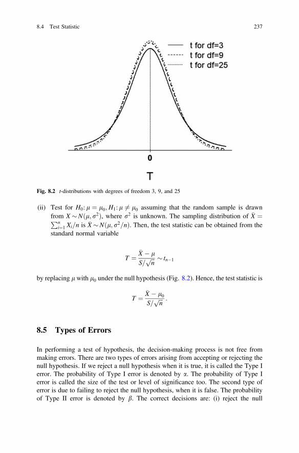
(ii) Test for H0: l ¼ l0;H1: l 6¼ l0 assuming that the random sample is drawnfrom X �Nðl; r2Þ, where r2 is unknown. The sampling distribution of �X ¼Pn
i¼1 Xi=n is �X�N l; r2=nð Þ. Then, the test statistic can be obtained from thestandard normal variable
T ¼�X � lS=
ffiffiffin
p � tn�1
by replacing lwith l0 under the null hypothesis (Fig. 8.2). Hence, the test statistic is
T ¼�X � l0S=
ffiffiffin
p :
8.5 Types of Errors
In performing a test of hypothesis, the decision-making process is not free frommaking errors. There are two types of errors arising from accepting or rejecting thenull hypothesis. If we reject a null hypothesis when it is true, it is called the Type Ierror. The probability of Type I error is denoted by a. The probability of Type Ierror is called the size of the test or level of significance too. The second type oferror is due to failing to reject the null hypothesis, when it is false. The probabilityof Type II error is denoted by b. The correct decisions are: (i) reject the null
Fig. 8.2 t-distributions with degrees of freedom 3, 9, and 25
8.4 Test Statistic 237

hypothesis if the null hypothesis is false, and (ii) failing to reject the null hypothesisif the null hypothesis is true. In performing a test, our goal is to keep both the Type Iand II errors minimum or in many instances a fixed. These decisions can be shownin a 2� 2 table as shown below.
Condition of null hypothesis H0
H0 is true H0 is false
Possible action (decision) Fail to reject H0 Correct decision Type II error
Reject H0 Type I error Correct decision
We can define this decision procedure more precisely using the conditionalprobabilities as summarized below.
(i) P ðType I errorÞ ¼ P ðreject H0 H0 is trueÞ ¼ ajThis probability statement shows the chance of rejecting a null hypothesis when inreality the null hypothesis is true. This probability is fixed at the pre-experimentstage and the rejection region is determined by the Type I error rate. In order tocontrol the overall erroneous rejections, the Type I error rate is fixed at a low levelbefore the experiment is conducted.
(ii) P ðType II errorÞ ¼ Pðfail to reject H0 H0 is falseÞ ¼ bjIn the above probability statement, the chance of failing to reject a null hypothesiswhen it might be false is stated. This probability should be kept as low as possible.
(iii) P ðfail to reject H0 H0 is trueÞ ¼ 1� ajThe above probability statement shows the chance of failure to reject a null hy-pothesis, when it is true that results in a correct decision of non-rejection of the nullhypothesis if given that the null hypothesis is true. If the probability of Type I erroris fixed then the complementary event of not making an error by non-rejection ofthe null hypothesis is also fixed at the pre-experiment stage.
(iv) P ðreject H0 H0 is falseÞ ¼ 1� bjThe probability of rejecting a null hypothesis when it is truly false is stated in (iv).This is the probability of making a right decision by rejecting the null hypothesiswhen it might be false. This probability is called the power of the test.
The probabilities of correct decisions, subject to the condition that the under-lying null and alternative hypotheses values are known, are shown in (iii) fornon-rejection of a null hypothesis if it is true, and in (iv) for rejection of a nullhypothesis if it is false. It has to be remembered here that underlying populationvalue is not known generally in most of the cases, but we may consider a hypo-thetical value based on which the test is performed. So when we say that the nullhypothesis is given to be true or false it provides only a hypothetical statementabout the population value, there might be other competing null hypothesis valuesthat could be tested with equal importance in many cases. Hence, the test is
238 8 Hypothesis Testing

conducted under a hypothetical situation about the underlying population and in arelative sense, the probability statements leading to specific decisions about thepopulation value reflect only one of the many hypothetical situations. We try to usea test for which the probability of correct decisions (iii) and (iv) are maximized. Ifwe decrease the probability of one type of error it may increase the probability ofother types of error for a fixed sample size. However, both the probabilities ofType I and Type II errors will decrease with an increase in sample size. Usually weconsider a fixed probability of Type I error, a. The probability of non-rejection ofthe null hypothesis if it is true is used in constructing a confidence interval asconfidence level or confidence coefficient. Similarly, the probability of rejecting anull hypothesis when it is false is called the power of a test and by increasing thepower of a test we try to minimize the Type II error.
8.6 Non-rejection and Critical Regions
The non-rejection and critical regions are defined on the basis of the null andalternative hypotheses as well as the test statistic. It is shown that the test statistic isalso a variable and there is sampling distribution from which we can find theprobabilities of greater than or smaller than some specified values of the teststatistic. The specification of these values are based on two criteria: (i) the alter-native hypothesis, one-sided or two-sided, and (ii) specification of Type I error, a. Ifthe test is one-sided, then based on the alternative hypothesis, we may define thecritical region either to the left or to the right side of the sampling distribution of thetest statistic. On the other hand, if the test is two-sided then the critical region isdefined to both the left- and right-hand sides of the sampling distribution of the teststatistic. The critical region may be defined as the region of a sample space with theproperty that if the observed value of a test statistic for testing a null hypothesisagainst an alternative falls in that region then the null hypothesis is rejected.Depending on the alternative hypothesis, the critical region is defined on one orboth sides of the sampling distribution of a test statistic. The non-rejection regionmay be defined as the region with the property that if the observed value of a teststatistic for testing a null hypothesis against an alternative falls in that region thenthe null hypothesis is not rejected. It implies that the non-rejection region is theregion under the sampling distribution complementary to the critical region. Thevalue of the test statistic that separates the critical region and non-rejection region iscalled a critical value for a one-sided test and there are two critical values for atwo-sided test. The level of significance, a, determines the size of a test and thecritical region depends on the choice of a. Usually, the choices of a are 0.05, 0.01 orin some cases 0.001.
8.5 Types of Errors 239

8.7 p-Value
Let us consider a test statistic, Z, to test the null hypothesis H0: l ¼ l0 against thealternative hypothesis H1: l[ l0 for a random sample of size n.
Instead of a fixed size of a test, sometimes many users prefer to use a p-value toreport the result of a test. Currently, there is a debate in the statistical communityregarding the conclusions based on statistical significance by using the p-valuewhich is commonly misused and misinterpreted (Wasserstein and Lazar 2016).Although it is used by the applied statisticians widely, statisticians may disagree insome situations on its appropriate use and on its interpretation as a measure ofevidence (Goodman 1992; Hung et al. 1997). In their ASA’s statement on p-values,context, process, and purpose, Wasserstein and Lazar (2016) defined informally thata p-value is the probability under a specified statistical model that a statisticalsummary of the data would be equal to or more extreme than its observed value.The p-value is a random variable derived from the test statistic and used for testinga null hypothesis in analyzing a set of data. According to Hung et al. (1997), “the p-value is derived from the perspective of a test of hypothesis in which a test statisticis calculated from results of a given set of data and, under the assumption that thenull hypothesis is true, the distribution of the test statistic is used to obtain the tailprobability of observing that result or a more extreme result.” The probability ofType I error, a, is a pre-experiment error rate that determines the rejection regionand the purpose of the fixed Type I error is to control the overall frequency ofmaking erroneous rejections of the null hypothesis.
Some principles of p-values stated in the ASA’s statement on p-values arequoted from Wasserstein and Lazar (2016)
(i) “P-values can indicate how incompatible the data are with a specified sta-tistical model.
(ii) P-values do not measure the probability that the studied hypothesis is true, orthe probability that the data were produced by random chance alone.
(iii) Scientific conclusions and business or policy decisions should not be basedonly on whether a p-value passes a specific threshold.
(iv) A proper inference requires full reporting and transparency.(v) A p-value, or statistical significance, does not measure the size of an effect or
the importance of a result.(vi) By itself, a p-value does not provide a good measure of evidence regarding a
model or hypothesis.”
In case of a test statistic employed to test a null hypothesis against an alternativehypothesis, p-value is the probability of the test statistic under null hypothesiswould be equal to or more extreme than its observed value. Let us consider anexample to illustrate the computation of p-values.
Example 1: For testing a null hypothesis H0: l ¼ l0 against an alternativehypothesis H1: l 6¼ l0 assuming that the random sample ðX1; . . .;XnÞ is from apopulation X�Nðl; r2Þ. The test statistic is
240 8 Hypothesis Testing

Z ¼�X � l0r=
ffiffiffin
p
and the sampling distribution of Z is Z�Nð0; 1Þ. Then, the observed values ofrandom samples are X1 ¼ x1; . . .;Xn ¼ xn and the sample mean is
�x ¼Pn
i¼1 xin
:
Now, we can obtain the value of the test statistic for the given sample and underthe null hypothesis as
z ¼ �x� l0r=
ffiffiffin
p :
Then, we can define the p-value as the probability under a specified statisticalhypothesis that the test statistic value from the data would be equal to or moreextreme than its observed value stated by
p-value ¼ PðZ[ zj jÞ þPðZ\� zj jÞ:
Here, the absolute value of z is used to define the tail areas for observed value ormore extreme values to both the tail areas in case of either a negative or a positivevalue of the test statistic. In case of a two-sided alternative, more extreme values ofthe test statistic can be obtained from the left or right tail areas of the samplingdistribution. For a positive value of z, it can be shown directly as
p-value ¼ PðZ[ zÞþPðZ\� zÞ
because the standard normal distribution is symmetric and the tail areas are greaterthan z and less than −z. Similarly, for a negative value of z, the p-value for thetwo-sided test is (Fig. 8.3)
Fig. 8.3 Figure displaying standard normal distribution with two-sided critical regions
8.7 p-Value 241
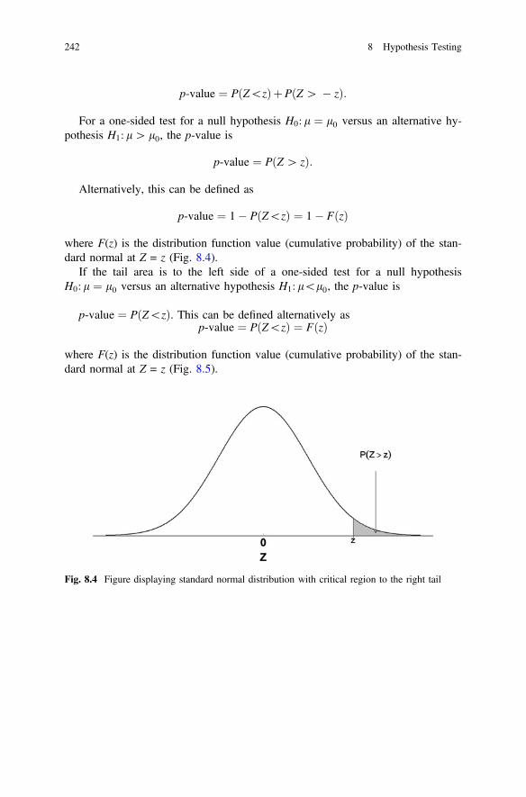
p-value ¼ PðZ\zÞþPðZ[ � zÞ:
For a one-sided test for a null hypothesis H0: l ¼ l0 versus an alternative hy-pothesis H1: l[ l0, the p-value is
p-value ¼ PðZ[ zÞ:
Alternatively, this can be defined as
p-value ¼ 1� PðZ\zÞ ¼ 1� FðzÞ
where F(z) is the distribution function value (cumulative probability) of the stan-dard normal at Z = z (Fig. 8.4).
If the tail area is to the left side of a one-sided test for a null hypothesisH0: l ¼ l0 versus an alternative hypothesis H1: l\l0, the p-value is
p-value ¼ PðZ\zÞ. This can be defined alternatively asp-value ¼ PðZ\zÞ ¼ FðzÞ
where F(z) is the distribution function value (cumulative probability) of the stan-dard normal at Z = z (Fig. 8.5).
Fig. 8.4 Figure displaying standard normal distribution with critical region to the right tail
242 8 Hypothesis Testing

8.8 The Procedure of Testing H0 (Against HA)
The test procedure for not rejecting H0 or rejecting H0 involves the following steps:
Steps 1. Specify the statements for null and alternative hypotheses and the size ofthe test or level of significance, a.
Steps 2. Carefully note the following: (i) probability distribution of the randomvariable from which the sample is drawn, (ii) if X �Nðl; r2Þ and the testis about the population mean then whether the variance is known orunknown, and (iii) sample size, n, and whether the sample size is small orlarge. This step will vary depending on whether we consider a test formean, proportion or variance from single or multiple populations, and sizeof sample.
Steps 3. Find: (i) the point estimator of the parameter being tested, (ii) the sam-pling distribution of the point estimator, (ii) the test statistic and (iii) thesampling distribution of the test statistic.
Steps 4. Calculate the value of the test statistic from the data and find the criticalvalue to define the rejection region and non-rejection or acceptanceregion.
Steps 5. Make decision and interpret result based on whether the calculated valueof the test statistic falls in the critical region or non-rejection region.Alternatively, the p-value is computed by determining the probability ofobserved or more extreme values from the sampling distribution of the teststatistic.
Fig. 8.5 Figure displaying standard normal distribution with critical region to the right tail
8.8 The Procedure of Testing H0 (Against HA) 243

8.9 Hypothesis Testing: A Single Population Mean (l)
1. r2 is known
Suppose that X1; . . .;Xn is a random sample of size n from a distribution (orpopulation) with mean l and variance r2. Then, the steps of performing the test ofhypothesis regarding a single population mean are shown below.
Step 1: Let the null and alternative hypotheses are H0:l ¼ l0 versus H1: l 6¼ l0.The level of significance is a, say a ¼ 0:05.
Step 2: Two different cases are considered.Case 1: Let the probability distribution of X is X�Nðl; r2Þ for the random
sample X1; . . .;Xn and let us assume that r2 is known. Here the sample size is n,small or large.
Case 2: Alternatively, the random sample is drawn from a non-normal popula-tion with mean l and variance r2 and sample size is large.
Step 3: The point estimator of l is �X ¼Pn
i¼1Xi
n . The sampling distributions fortwo different cases specified in step 2 are
Case 1: �X�Nðl; r2=nÞ, the standard error of �X is r=ffiffiffin
p.
Case 2: For a large sample size, it can be shown asymptotically that�X � Nðl; r2=nÞ, the standard error of �X is r=
ffiffiffin
papproximately.
The statistic for both cases 1 and 2 is
Z ¼�X � lr=
ffiffiffin
p
where the sampling distribution of Z is Z�Nð0; 1Þ for case 1 and if the sample sizeis large then approximately Z � Nð0; 1Þ for case 2.
Step 4: The observed value of the test statistic from the sample data X1 ¼x1; . . .;Xn ¼ xn is
z ¼ �x� l0r=
ffiffiffin
p :
The critical values for a two-sided alternative are za=2 and z1�a=2 (Fig. 8.6).Step 5: If z\za=2 or z[ z1�a=2 then the test statistic value from the sample data
falls in the rejection region and the decision is in favor of rejecting the null hy-pothesis. On the other hand, if z[ za=2 and z\z1�a=2 then the test statistic falls inthe non-rejection region. In this case, the decision is in favor of non-rejection of nullhypothesis as evident from the sample data (Fig. 8.7).
2. r2 is unknown
Let us consider that X1; . . .;Xn be a random sample of size n from a normaldistribution (or population) with mean l and variance r2 where r2 is not known.
244 8 Hypothesis Testing

The steps of performing the test of hypothesis regarding a single population meanare shown below.
Step 1: The null and alternative hypotheses are H0: l ¼ l0 versus H1: l 6¼ l0.The level of significance is a, say a ¼ 0:05.
Step 2: Two different cases are considered.Case 1: Let us assume that the probability distribution of X is X�Nðl; r2Þ for
the random sample X1; . . .;Xn and let r2 be unknown. The sample size n is small.Case 2: Alternatively, the random sample is drawn from a normal population
with mean l and variance r2 and sample size is large.
Step 3: The point estimator of l is �X ¼Pn
i¼1Xi
n . The sampling distributions fortwo different cases specified in step 2 are
Fig. 8.7 Figure displaying standard normal distribution with non-rejection and rejection regions
Fig. 8.6 Figure displaying standard normal distribution with critical values for two-sidedalternative
8.9 Hypothesis Testing: A Single Population Mean (l) 245

Case 1: �X�Nðl; r2=nÞ, the standard error of �X is r=ffiffiffin
p.
Case 2: For a large sample size, it can be shown asymptotically that�X � Nðl; r2=nÞ, the standard error of �X is r=
ffiffiffin
papproximately.
The test statistic for case 1 is
T ¼�X � l0S=
ffiffiffin
p
where r is replaced by its estimator S and the sampling distribution of T is T � tn�1
for case 1 and if the sample size is large then T is approximately standard normaland can be expressed as Z � Nð0; 1Þ for case 2.
Step 4: The observed value of the test statistics for cases 1 and 2 from the sampledata X1 ¼ x1; . . .;Xn ¼ xn are
Case 1: t ¼ �x�l0s=ffiffin
p
The critical values for a two-sided alternative are tðn�1Þ;a=2 and tðn�1Þ;1�a=2.
Case 2: z ¼ �x�l0s=ffiffin
p
The critical values for a two-sided alternative are za=2 and z1�a=2.Step 5: The decision for cases 1 and 2 can be made as follows:Case 1: It is mentioned that case 1 represents a random sample drawn from
normal population, where the population variance is unknown. Then to perform thetest for the population mean, we have considered a t-test statistic with (n − 1)degrees of freedom. If t\tðn�1Þ;a=2 or t[ tðn�1Þ;1�a=2, then the test statistic valuefrom the sample data falls in the rejection region and the decision is in favor ofrejecting the null hypothesis. However, if tðn�1Þ;a=2\t\tðn�1Þ;1�a=2 then the teststatistic falls in the non-rejection region. In this case, the decision based on thesample data is in favor of non-rejection of the null hypothesis (Fig. 8.8).
Fig. 8.8 Figure displaying t-distribution with non-rejection and rejection regions
246 8 Hypothesis Testing

Case 2: In this case also the random sample is assumed to be drawn from anormal population with variance unknown. Then, the test statistic tends to follow astandard normal distribution for a large sample size. If the value of the test statisticis z\za=2 or z[ z1�a=2, then the sample data favor rejection of the null hypothesisbecause the test statistic value from sample data falls in the critical or rejectionregion. If za=2\z\z1�a=2 then the test statistic falls in the non-rejection region andthe decision is in favor of non-rejection of null hypothesis.
Example 8.1 Test for l, r2 is known.The example we have employed to illustrate the confidence interval for popu-
lation mean for known population variance is used here. In that example, we haveconsidered a random sample of 123 patients admitted to a hospital with old agecomplications. The sample mean age is 55 years. The population variance isassumed to be r2 ¼ 82. Let us assume that the population is normal with mean land variance r2 ¼ 82. Then a test is performed to know whether the populationmean is l ¼ 50.
In this example, X1; . . .;Xn is a random sample of size n from a distribution (orpopulation) with mean l and variance r2.
Step 1: The null and alternative hypotheses are
H0: l ¼ 50 versus H1:l 6¼ 50:
The level of significance is a ¼ 0:05.Step 2: The probability distribution of X is X�Nðl; r2Þ for the random sample
X1; . . .;Xn and let us assume that r2 is known.
Step 3: The point estimator of l is �X ¼Pn
i¼1Xi
n and its sampling distribution is�X�Nðl; r2=nÞ, the standard error of �X is r=
ffiffiffin
p.
The statistic is
Z ¼�X � lr=
ffiffiffin
p
where the sampling distribution of Z is Z �Nð0; 1Þ.Step 4: The observed value of the test statistic from the sample data is
z ¼ �x� l0r=
ffiffiffin
p ¼ 55� 50
9:06=ffiffiffiffiffiffiffiffi123
p ¼ 50:8169
¼ 6:1207:
The critical values for a two-sided alternative are z0:025 ¼ �196 and z0:975 ¼1:96 (Fig. 8.9).
Step 5: The calculated value of the test statistic is 6.1207 which is greater thanthe critical value, i.e., z[ z0:975 where z = 6.1207 and z0:975 ¼ 1:96. It shows thatthe test statistic value from the sample data falls in the rejection region and thedecision is in favor of rejecting the null hypothesis.
8.9 Hypothesis Testing: A Single Population Mean (l) 247

Example 8.2 Test for l, r2 is unknown.Using the data on height of women in their adulthood presented in Chap. 7, an
example for test on population mean (when r2 is unknown) is shown here.A hypothetical sample of 24 women considered here is assumed to be drawn from anormal distribution with population mean l and variance r2. The sample mean andvariance of height of the selected women are 151 cm and 18.65 cm2 respectively.Then, let us test for the null hypothesis whether population mean is 153 cm or not.
SolutionThe random sample X1; . . .;Xn is assumed to be drawn from a normal distributionwith mean l and variance r2 where r2 is not known.
Step 1: The null and alternative hypotheses areH0: l ¼ 153 versus H1: l 6¼ 153. The level of significance is a ¼ 0:05.Step 2: The probability distribution of X is X�Nðl; r2Þ for the random sample
X1; . . .;Xn and let r2 be unknown. The sample size n is small.
Step 3: The point estimator of l is �X ¼Pn
i¼1Xi
n and�X�Nðl; r2=nÞ, the standard error of �X is r=
ffiffiffin
p.
The test statistic is
T ¼�X � l0S=
ffiffiffin
p
and the sampling distribution of T is T � tn�1,Step 4: The observed value of the test statistics is
t ¼ �x� l0s=
ffiffiffin
p ¼ 151� 153
4:32=ffiffiffiffiffi24
p ¼ �20:8818
¼ �2:2681
Fig. 8.9 Figure displaying critical regions for test about population mean, when variance isknown
248 8 Hypothesis Testing

where n = 24 and s ¼ þffiffiffiffis2
p¼ þ ffiffiffiffiffiffiffiffiffiffiffi
18:65p ¼ 4:32.
The critical values for a two-sided alternative are t23;0:025 ¼ �2:067 and t23;0:975 ¼2:067 (Fig. 8.10).
Step 5: The calculated value of the test statistic, t, appears to be less than thecritical value at the lower tail, i.e., t\tðn�1Þ;a=2 , hence the test statistic value fromthe sample data falls in the rejection region and the decision is in favor of rejectingthe null hypothesis.
8.10 Hypothesis Testing: The Difference Between TwoPopulation Means: Independent Populations
Suppose that we have two independent populations where the first population ischaracterized with parameters mean = l1 and variance = r21 and the second pop-ulation with mean = l2 and variance = r22. The random samples from the first andsecond populations are X11; . . .;X1n1ð Þ and X21; . . .;X2n2ð Þ respectively. Let usdenote the probability distributions for the variables for the first and second randomsamples as X1 �Dðl1; r21Þ and X2 �Dðl2;r22Þ, respectively, where D representsunderlying population distribution. Here, we are interested in comparing l1 and l2,or equivalently, making inferences about the difference between the meansðl1 � l2Þ. Let us select a random sample of size n1 from the first population andanother random sample of size n2 from the second population independently and let�X1 and S21 be the sample mean and the sample variance of the first random sampleand �X2 and S22 be the sample mean and the sample variance of the second randomsample. The sampling distribution of �X1 � �X2 is used to make inferences aboutðl1 � l2Þ.
Fig. 8.10 Figure displaying critical regions for test about population mean when variance isunknown
8.9 Hypothesis Testing: A Single Population Mean (l) 249

The steps discussed in the previous section can be used to illustrate the testing ofhypothesis of difference between two population means. The steps are highlightedbelow.
1. r21 and r22 are known
Suppose that the random samples from the first population is X11; . . .;X1n1ð Þ withsample size n1 and the random sample from the second population is X21; . . .;X2n2ð Þwith sample size n2.
Step 1: The null and alternative hypotheses are H0: l1 � l2 ¼ 0 versusH1: l1 � l2 6¼ 0. The level of significance is a, say a ¼ 0:05.
Step 2: Two different cases are considered.Case 1: Let the probability distribution of X1 is X1 �Nðl1; r21Þ for the random
sample X11; . . .;X1n1 and X2 is X2 �Nðl2;r22Þ for the random sample X21; . . .;X2n2
let us assume that r21 and r22 are known.Case 2: Alternatively, let the probability distribution of X1 is non-normal for the
random sample X11; . . .;X1n1 with mean l1 and variance r21 and X2 is non-normalfor the random sample X21; . . .;X2n2 with mean l2 and variance r22 for the randomsample X21; . . .;X2n2 . Let us assume that r21 and r22 are known and sample sizes forboth the samples are large.
Step 3: The point estimator of l1 is �X1 ¼Pn1
i¼1X1i
n1and l2 is �X2 ¼
Pn2i¼1
X2i
n2. The
sampling distributions of �X1 � �X2 for two different cases specified in step 2 aresummarized below.
Case 1: �X1 � �X2 �Nðl1 � l2; r21=n1 þ r22=n2Þ and the standard error of
�X1 � �X2 is r1=ffiffiffiffiffin1
p þ r2=ffiffiffiffiffin2
p.
Case 2: For large sample, it can be shown asymptotically that
�X1 � �X2 � Nðl1 � l2; r21=n1 þ r22=n2Þ and the standard error
of �X1 � �X2 is approximately r1=ffiffiffiffiffin1
p þ r2=ffiffiffiffiffin2
p.
The statistic for both cases 1 and 2 is
Z ¼�X1 � �X2 � ðl1 � l2Þffiffiffiffiffiffiffiffiffiffiffiffiffiffiffiffiffiffiffiffiffiffiffiffiffiffiffiffi
r21=n1 þ r22=n2p
where the sampling distribution of Z is Z�Nð0; 1Þ for case 1 and if the samplesizes are large then approximately Z � Nð0; 1Þ for case 2.
Step 4: The observed value of the test statistic from the sample data X11 ¼x11; . . .;X1n1 ¼ x1n1 for sample 1 and X21 ¼ x21; . . .;X2n1 ¼ x2n2 for sample 2 is
250 8 Hypothesis Testing
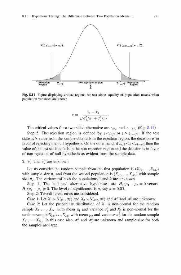
z ¼ �x1 � �x2ffiffiffiffiffiffiffiffiffiffiffiffiffiffiffiffiffiffiffiffiffiffiffiffiffiffiffiffir21=n1 þ r22=n2
p :
The critical values for a two-sided alternative are za=2 and z1�a=2 (Fig. 8.11).Step 5: The rejection region is defined by z\za=2 or z[ z1�a=2. If the test
statistic’s value from the sample data falls in the rejection region, the decision is infavor of rejecting the null hypothesis. On the other hand, if za=2\z\z1�a=2 then thevalue of the test statistic falls in the non-rejection region and the decision is in favorof non-rejection of null hypothesis as evident from the sample data.
2. r21 and r22 are unknown
Let us consider the random sample from the first population is X11; . . .;X1n1ð Þwith sample size n1 and from the second population is X21; . . .;X2n2ð Þ with samplesize n2. The variance of both the populations 1 and 2 are unknown.
Step 1: The null and alternative hypotheses are H0: l1 � l2 ¼ 0 versusH1: l1 � l2 6¼ 0. The level of significance is a, say a ¼ 0:05.
Step 2: Two different cases are considered.Case 1: Let X1 �Nðl1; r21Þ and X2 �Nðl2; r22Þ and r21 and r22 are unknown.Case 2: Let the probability distribution of X1 is non-normal for the random
sample X11; . . .;X1n1 with mean l1 and variance r21 and X2 is non-normal for therandom sample X21; . . .;X2n2 with mean l2 and variance r22 for the random sampleX21; . . .;X2n2 . In this case also, r21 and r22 are unknown and sample size for boththe samples are large.
Fig. 8.11 Figure displaying critical regions for test about equality of population means whenpopulation variances are known
8.10 Hypothesis Testing: The Difference Between Two Population Means … 251

Step 3: The point estimators of population means: the estimator of l1 is �X1 ¼Pn1i¼1
X1i
n1and the estimator of l2 is �X2 ¼
Pn2i¼1
X2i
n2. The sampling distribution of �X1 �
�X2 for 1 and 2 are summarized below.Case 1: �X1 � �X2 �Nðl1 � l2; r
21=n1 þ r22=n2Þ.
Case 2: For large sample, it can be shown asymptotically that
�X1 � �X2 � Nðl1 � l2; r21=n1 þ r22=n2Þ:
The test statistic for case 1 is
T ¼�X1 � �X2ffiffiffiffiffiffiffiffiffiffiffiffiffiffiffiffiffiffiffiffiffiffiffiffiffiffiffiffi
S21=n1 þ S22=n2p
where the sampling distribution of T is T � tm for case 1.The denominator of T shown above, which is the standard error of the estimators
of two population means, may be estimated under different assumptions about thepopulation variances. We address two different situations here.
Case 1(i) The population variances of two independent populations are unknownbut assumed to be equal which imply r21 ¼ r22 ¼ r2. The sample variances aredefined as
S21 ¼Pn1
i¼1 X1i � �X1ð Þ2n1 � 1
and S22 ¼Pn2
i¼1 X2i � �X2ð Þ2n2 � 1
:
For equality of population variances a pooled estimator of population variance ispreferred as shown below
S2p ¼Pn1
i¼1 X1i � �X1ð Þ2 þ Pn2i¼1 X2i � �X2ð Þ2
n1 þ n2 � 2¼ ðn1 � 1ÞS21 þðn2 � 1ÞS22
n1 þ n2 � 2:
Under this assumption of equality of variances, the test statistic is redefined as
T ¼�X1 � �X2
Spffiffiffiffiffiffiffiffiffiffiffiffiffiffiffiffiffiffiffiffiffiffiffiffiffiffiffiffiffiffiffið1=n1Þþ ð1=n2Þ
p :
Here, T is T � tm and the degrees of freedom m ¼ n1 þ n2 � 2.Case 1(ii) If the population variances are assumed to be unequal and unknown
then we have to deal with r21 6¼ r22 and the pooled estimator of the variance can notbe used. In this case, the test statistic is
252 8 Hypothesis Testing

T ¼�X1 � �X2ffiffiffiffiffiffiffiffiffiffiffiffiffiffiffiffiffiffiffiffiffiffiffiffiffiffiffiffi
S21=n1 þ S22=n2p
where the sampling distribution of T is T � tm as shown earlier and the degrees offreedom is obtained by using the following approximation popularly known as theSatterthwaite approximation introduced in 1946 (Satterthwaite 1946)
m ¼ s21=n1 þ s22=n2� �2
s21=n1� �2
=ðn1 � 1Þh i
þ s22=n2� �2
=ðn2 � 1Þh i :
Usually, this approximation is not an integer and we can approximate thedegrees of freedom by rounding the result to the nearest integer.
The test statistic for case 2 is
Z ¼�X1 � �X2ffiffiffiffiffiffiffiffiffiffiffiffiffiffiffiffiffiffiffiffiffiffiffiffiffiffiffiffi
S21=n1 þ S22=n2p
where the sampling distribution of Z is asymptotically Z � Nð0; 1Þ if sample sizesare large for case 2.
Step 4: The values of the test statistics for cases 1 and 2 are shown below.The value of the test statistic from sample data for case 1(i) is
t ¼ �x1 � �x2sp
ffiffiffiffiffiffiffiffiffiffiffiffiffiffiffiffiffiffiffiffiffiffiffiffiffiffiffiffiffiffiffið1=n1Þþ ð1=n2Þp
and the critical values for the two-tailed test at the left and right tail areas aretn1 þ n2�2;a and tn1 þ n2�2;1�a:
Similarly, the test statistic from sample data for case 1(ii) is
t ¼ �x1 � �x2ffiffiffiffiffiffiffiffiffiffiffiffiffiffiffiffiffiffiffiffiffiffiffiffiffiffiffis21=n1 þ s22=n2
p :
The critical values are tm;a and tm;1�a, where the degrees of freedom, m, is
m ¼ s21=n1 þ s22=n2� �2
s21=n1� �2
=ðn1 � 1Þh i
þ s22=n2� �2
=ðn2 � 1Þh i :
For case 2, the value of the test statistic for large sample size is
z ¼ �x1 � �x2ffiffiffiffiffiffiffiffiffiffiffiffiffiffiffiffiffiffiffiffiffiffiffiffiffiffiffiffir21=n1 þ r22=n2
p :
The critical values for a two-sided alternative are za=2 and z1�a=2. Here, thesampling distribution of Z is asymptotically Z � Nð0; 1Þ if sample sizes are large.
8.10 Hypothesis Testing: The Difference Between Two Population Means … 253
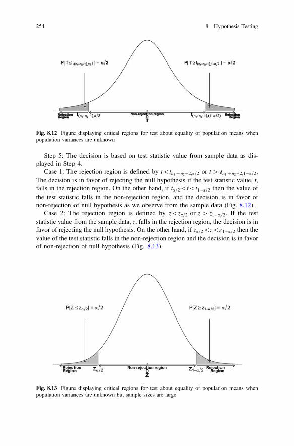
Step 5: The decision is based on test statistic value from sample data as dis-played in Step 4.
Case 1: The rejection region is defined by t\tn1 þ n2�2;a=2 or t[ tn1 þ n2�2;1�a=2.The decision is in favor of rejecting the null hypothesis if the test statistic value, t,falls in the rejection region. On the other hand, if ta=2\t\t1�a=2 then the value ofthe test statistic falls in the non-rejection region, and the decision is in favor ofnon-rejection of null hypothesis as we observe from the sample data (Fig. 8.12).
Case 2: The rejection region is defined by z\za=2 or z[ z1�a=2. If the teststatistic value from the sample data, z, falls in the rejection region, the decision is infavor of rejecting the null hypothesis. On the other hand, if za=2\z\z1�a=2 then thevalue of the test statistic falls in the non-rejection region and the decision is in favorof non-rejection of null hypothesis (Fig. 8.13).
Fig. 8.12 Figure displaying critical regions for test about equality of population means whenpopulation variances are unknown
Fig. 8.13 Figure displaying critical regions for test about equality of population means whenpopulation variances are unknown but sample sizes are large
254 8 Hypothesis Testing
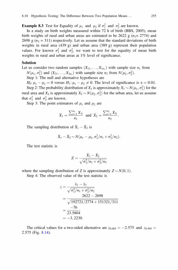
Example 8.3 Test for Equality of l1 and l2 if r21 and r22 are known.In a study on birth weights measured within 72 h of birth (BBS, 2005), mean
birth weights of rural and urban areas are estimated to be 2622 g (n1= 2774) and2698 g (n2 = 311) respectively. Let us assume that the standard deviations of birthweights in rural area (439 g) and urban area (389 g) represent their populationvalues. For known r21 and r22, we want to test for the equality of mean birthweights in rural and urban areas at 1% level of significance.
SolutionLet us consider two random samples X11; . . .;X1n1ð Þ with sample size n1 from
Nðl1; r21Þ and X21; . . .;X2n2ð Þ with sample size n2 from Nðl2; r22Þ.Step 1: The null and alternative hypotheses areH0: l1 � l2 ¼ 0 versus H1: l1 � l2 6¼ 0. The level of significance is a ¼ 0:01:Step 2: The probability distribution of X1 is approximately X1 �Nðl1; r21Þ for the
rural area and X2 is approximately X2 �Nðl2; r22Þ for the urban area, let us assumethat r21 and r22 are known.
Step 3: The point estimators of l1 and l2 are
�X1 ¼Pn1
i¼1 X1i
n1and �X2 ¼
Pn2i¼1 X2i
n2:
The sampling distribution of �X1 � �X2 is
�X1 � �X2 �Nðl1 � l2; r21=n1 þ r22=n2Þ:
The test statistic is
Z ¼�X1 � �X2ffiffiffiffiffiffiffiffiffiffiffiffiffiffiffiffiffiffiffiffiffiffiffiffiffiffiffiffi
r21=n1 þ r22=n2p
where the sampling distribution of Z is approximately Z�Nð0; 1Þ.Step 4: The observed value of the test statistic is
z ¼ �x1 � �x2ffiffiffiffiffiffiffiffiffiffiffiffiffiffiffiffiffiffiffiffiffiffiffiffiffiffiffiffir21=n1 þ r22=n2
p¼ 2622� 2698ffiffiffiffiffiffiffiffiffiffiffiffiffiffiffiffiffiffiffiffiffiffiffiffiffiffiffiffiffiffiffiffiffiffiffiffiffiffiffiffiffiffiffiffiffiffiffiffiffiffiffiffiffiffiffiffi
192721=2774þ 151321=311p
¼ �7623:5804
¼ �3; 2230:
The critical values for a two-sided alternative are z0:005 ¼ �2:575 and z0:995 ¼2:575 (Fig. 8.14).
8.10 Hypothesis Testing: The Difference Between Two Population Means … 255

Step 5: The rejection region is defined by z\z0:005 or z[ z0:995 and as the valueof the test statistic from the sample data falls in the rejection region, the decision isin favor of rejecting the null hypothesis of equality of the birth weights in rural andurban areas.
Example 8.4 Test for Equality of l1 and l2 if r21 and r22 are unknown.
Case 1 r21 and r22 are unknown but Assumed to be Equal.In a study on heights, two samples of height of women are drawn randomly from
normal populations with means l1 and l2 and variances r21 and r22 respectively.The size of sample 1 is 28 and sample 2 is 24. The sample 1 mean and variance are151.88 cm and 26.53 cm2 and sample 2 mean and variance are 150.99 cm and18.65 cm2. It is of interest to test the equality of two population means if populationvariances are unknown.
SolutionThe sample from the first population is X11; . . .;X1n1ð Þ with sample size n1 and fromthe second population is X21; . . .;X2n2ð Þ with sample size n2. The variance of boththe populations 1 and 2 are unknown.
Step 1: The null and alternative hypotheses areH0: l1 � l2 ¼ 0 versus H1: l1 � l2 6¼ 0.The level of significance is a ¼ 0:05.Step 2: Let X1 �Nðl1; r21Þ and X2 �Nðl2; r22Þ and r21 and r22 are unknown.
Step 3: The point estimator l1 is �X1 ¼Pn1
i¼1X1i
n1and l2 is �X2 ¼
Pn2i¼1
X2i
n2. The
sampling distribution of �X1 � �X2 is
Fig. 8.14 Figure displaying critical regions for test about equality of population means whenpopulation variances are known
256 8 Hypothesis Testing

�X1 � �X2 �Nðl1 � l2; r21=n1 þ r22=n2Þ:
The test statistic is
T ¼�X1 � �X2ffiffiffiffiffiffiffiffiffiffiffiffiffiffiffiffiffiffiffiffiffiffiffiffiffiffiffiffi
S21=n1 þ S22=n2p
where the sampling distribution of T is T � tm.If the population variances of two independent populations are unknown but
assumed to be equal which imply r21 ¼ r22 ¼ r2. The estimator of the pooledvariance under the assumption of equality of population variances is
S2p ¼Pn1
i¼1 X1i � �X1ð Þ2 þ Pn2i¼1 X2i � �X2ð Þ2
n1 þ n2 � 2¼ ðn1 � 1ÞS21 þðn2 � 1ÞS22
n1 þ n2 � 2:
The test statistic is redefined as
T ¼�X1 � �X2
Spffiffiffiffiffiffiffiffiffiffiffiffiffiffiffiffiffiffiffiffiffiffiffiffiffiffiffiffiffiffiffið1=n1Þþ ð1=n2Þ
p :
Here, T is T � tm and the degrees of freedom m ¼ n1 þ n2 � 2.Step 4: The values of the test statistic is
t ¼ �x1 � �x2sp
ffiffiffiffiffiffiffiffiffiffiffiffiffiffiffiffiffiffiffiffiffiffiffiffiffiffiffiffiffiffiffið1=n1Þþ ð1=n2Þp ;
where
l1 � l2 ¼ �x1 � �x2 ¼ 151:88� 150:99 ¼ 0:89;
s2p ¼ðn1 � 1Þs21 þðn2 � 1Þs22
n1 þ n2 � 2
¼ 27� 26:53þ 23� 18:6550
¼ 23:45;
and sp ¼ 4:84.The value of t is
t ¼ �x1 � �x2sp
ffiffiffiffiffiffiffiffiffiffiffiffiffiffiffiffiffiffiffiffiffiffiffiffiffiffiffiffiffiffiffið1=n1Þþ ð1=n2Þp
¼ 0:89
4:84ffiffiffiffiffiffiffiffiffiffiffiffiffiffiffiffiffiffiffiffiffiffiffiffiffiffiffiffiffiffiffiffið1=28Þþ ð1=24Þp
¼ 0:6610:
8.10 Hypothesis Testing: The Difference Between Two Population Means … 257

The critical values for the two-tailed test at the left and right tail areas aret50;0:025 ¼ �2:009 and t50;0:975 ¼ 2:009 (Fig. 8.15).
Step 5: The non-rejection region is defined by ta=2\t\t1�a=2. The decision is infavor of not rejecting the null hypothesis because the test statistic value, t, falls inthe non-rejection region. We may conclude that we may not reject the nullhypothesis of equality of mean heights of women from two different populations.
Example 8.5 Test for Equality of l1 and l2 if r21 and r22 are unknown andassumed to be unequal.
Case II r21 and r22 are unknown and assumed to be unequal.Let us consider that a study was conducted to collect data on weight of women in
two areas, denoted by area 1 and area 2. Using the data on weight from both thesamples we have found the mean weights of women in areas 1 and 2 are 48.68 and49.34 kg, respectively. The sample variances are 25.50 kg2 for area 1 and90.02 kg2 in area 2. We have to test for the equality of two population means ofwomen in areas 1 and 2 at 5% level of significance.
SolutionStep 1: The null and alternative hypotheses are
H0: l1 � l2 ¼ 0 versus H1:l1 � l2 6¼ 0:
The level of significance is a ¼ 0:05.Step 2: Let X1 �Nðl1; r21Þ and X2 �Nðl2; r22Þ, where r21 and r22 are unknown
and assumed to be unequal.
Fig. 8.15 Figure displaying critical regions for test about equality of population means whenpopulation variances are unknown
258 8 Hypothesis Testing

Step 3: The point estimators of population means the estimator of l1 is �X1 ¼Pn1i¼1
X1i
n1and the estimator of l2 is �X2 ¼
Pn2i¼1
X2i
n2. The sampling distribution of �X1 �
�X2 is �X1 � �X2 �Nðl1 � l2; r21=n1 þ r22=n2Þ.
The test statistic is
T ¼�X1 � �X2ffiffiffiffiffiffiffiffiffiffiffiffiffiffiffiffiffiffiffiffiffiffiffiffiffiffiffiffi
S21=n1 þ S22=n2p
where the sampling distribution of T is T � tm.The Satterthwaite approximation of degrees of freedom is
m ¼ s21=n1 þ s22=n2� �2
s21=n1� �2
=ðn1 � 1Þh i
þ s22=n2� �2
=ðn2 � 1Þh i
¼ 25:51=24þ 76:91=28ð Þ2
25:51=24ð Þ2=23h i
þ 76:91=28ð Þ2=27h i
¼ 25:51=24þ 76:91=28ð Þ2
25:51=24ð Þ2=23h i
þ 76:91=28ð Þ2=27h i
� 44:
Step 4: The test statistic from sample data is
t ¼ �x1 � �x2ffiffiffiffiffiffiffiffiffiffiffiffiffiffiffiffiffiffiffiffiffiffiffiffiffiffiffis21=n1 þ s22=n2
p¼ �0:72ffiffiffiffiffiffiffiffiffiffiffiffiffiffiffiffiffiffiffiffiffiffiffiffiffiffiffiffiffiffiffiffiffiffiffiffiffiffiffiffiffiffi
25:51=24þ 76:91=28p
¼ �0:3692
where the degrees of freedom is approximately 44. The critical values for thetwo-tailed test are t44;0:025 ¼ �2:0154 and t44;0:975 ¼ 2:0154 (Fig. 8.16).
Step 5: The decision is in favor of not rejecting the null hypothesis because thetest statistic value, t = 0.3692, falls in the non-rejection region, ta=2\t\t1�a=2.This decision implies that the null hypothesis of equality of weights of women inareas 1 and 2 may not be rejected.
8.10 Hypothesis Testing: The Difference Between Two Population Means … 259

8.11 Paired Comparisons
In this section, we are interested in comparing the means of two correlated variablesfrom normal populations. In other words, we wish to make statistical inference forthe difference between the means of two correlated normal populations. Paired t-testis used for testing the equality of the means of two related normal populations.Examples of related populations are: (i) height of the father and height of his son,(ii) weight of subjects before and after a diet program, (iii) pulse rate of patientbefore and after a medical treatment, (iv) hemoglobin level of the patient before andafter the medical treatment, etc. It is clear from the examples that data are observedin pairs. In a paired comparison, we perform a test to arrive at a decision whetherthere is any difference between the population means. In the before and afterreceiving a treatment experiments, if the difference in the means is not statisticallysignificant then it indicates that there is not much evidence in favor of rejecting thenull hypothesis of no difference in the correlated variables representing outcomesbefore and after the experiment is conducted.
Let us consider n pairs of a random sample X1; Y1ð Þ; . . .; ðXn;YnÞ and theobservations in the sample are x1; y1ð Þ; . . .; ðxn; ynÞ. We assume that the data arecontinuous and differences in the matched pairs follow a normal probability dis-tribution. It is noteworthy that the assumption of normality is required for thedifference in the pairs of variables, D ¼ X � Y , not for the original variables, X andY. The observed difference in pairs is denoted by d ¼ x� y.
Let us consider that the differences in pairs, Di ¼ Xi � Yi; i ¼ 1; . . .; n, follow anormal probability density with mean lD and variance r2D. The estimator for thepopulation mean of the differences is denoted by
Fig. 8.16 Figure displaying critical regions for test about equality of population means whenpopulation variances are unknown and unequal
260 8 Hypothesis Testing

�D ¼Pn
i¼1 Di
n
and the corresponding sample mean from the observed data is
�d ¼Pn
i¼1 din
:
Similarly, the sample variance of the differences for the random pairs is S2d ¼Pn
i¼1ðDi��DÞ2n�1 and the corresponding sample variance from the observed data is
s2d ¼Pn
i¼1ðdi��dÞ2
n�1
.
The steps of performing the test of hypothesis regarding the mean difference inthe pairs of variables are discussed below.
Step 1: The null and alternative hypotheses are H0: lD ¼ lX � lY =0versusH1: lD 6¼ 0. The level of significance is a, say a ¼ 0:05.
Step 2: Let us assume that the probability distribution of D is D�NðlD; r2DÞ forthe random sample of pairs ðX1; Y1Þ; . . .; ðXn; YnÞ and let r2D be unknown. Therandom sample is comprised of n pairs.
Step 3: The point estimator of lD is
�D ¼Pn
i¼1 Di
n:
The sampling distribution of �D is summarized below.
(i) Eð�DÞ ¼ Eð�X � �YÞ ¼ lX � lY ¼ lD,(ii) �D�NðlD; r2D=nÞ, the standard error of �D is rD=
ffiffiffin
p.
The test statistic for testing the difference in the means of the paired variables is
T ¼�D� lDSd=
ffiffiffin
p
where rD is replaced by its estimator Sd and the sampling distribution of T isT � tn�1.
Step 4: The observed value of the test statistic from the sample dataðx1; y1Þ; . . .; ðxn; ynÞ is
t ¼�d
sd=ffiffiffin
p
The critical values for a two-sided alternative are tðn�1Þ;a=2 and tðn�1Þ;1�a=2
(Fig. 8.17).
8.11 Paired Comparisons 261

Step 5: If t\tðn�1Þ;a=2 or t[ tðn�1Þ;1�a=2 then the test statistic value from thesample data falls in the rejection region and the decision is in favor of rejecting thenull hypothesis. However, if tðn�1Þ;a=2\t\tðn�1Þ;1�a=2 then the test statistic falls inthe non-rejection region. In this case, the decision based on the sample data is infavor of non-rejection of the null hypothesis.
Example 8.6 Paired t-test.Let us consider the following paired hypothetical data on 10 individuals dis-
playing their weights in kg before (X) and after (Y) a diet program was introduced inorder to find any possible change in weight of subjects of age 15–49 years attri-butable to the diet program.
Individual 1 2 3 4 5 6 7 8 9 10
x 53 51 43 59 55 39 50 42 53 51
y 50 50 45 53 52 42 51 40 50 52
The research question is whether the diet program could make any difference inthe weight of subjects. Consider a ¼ 0:05.
SolutionThe steps of a paired t-test are discussed below.
Step 1: The null and alternative hypotheses are
H0: lD ¼ lX � lY = 0 versus H1: lD 6¼ 0:
The level of significance is a ¼ 0:05.Step 2: It is assumed that the probability distribution of D is D�NðlD; r2DÞ,
where D = X − Y for pairs ðX1; Y1Þ; . . .; ðXn; YnÞ, and let r2D be unknown.
Fig. 8.17 Figure displaying critical regions for test about equality of population means usingpaired t-test
262 8 Hypothesis Testing
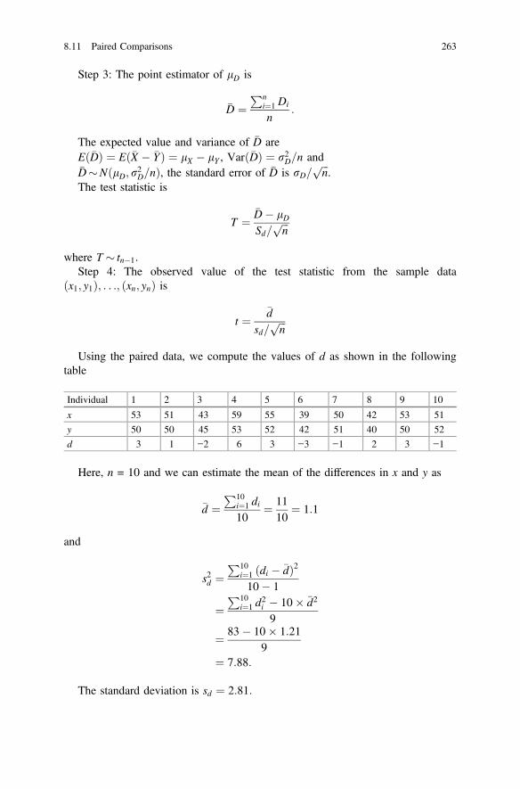
Step 3: The point estimator of lD is
�D ¼Pn
i¼1 Di
n:
The expected value and variance of �D areEð�DÞ ¼ Eð�X � �YÞ ¼ lX � lY , Varð�DÞ ¼ r2D=n and�D�NðlD; r2D=nÞ, the standard error of �D is rD=
ffiffiffin
p.
The test statistic is
T ¼�D� lDSd=
ffiffiffin
p
where T � tn�1.Step 4: The observed value of the test statistic from the sample data
ðx1; y1Þ; . . .; ðxn; ynÞ is
t ¼�d
sd=ffiffiffin
p
Using the paired data, we compute the values of d as shown in the followingtable
Individual 1 2 3 4 5 6 7 8 9 10
x 53 51 43 59 55 39 50 42 53 51
y 50 50 45 53 52 42 51 40 50 52
d 3 1 −2 6 3 −3 −1 2 3 −1
Here, n = 10 and we can estimate the mean of the differences in x and y as
�d ¼P10
i¼1 di10
¼ 1110
¼ 1:1
and
s2d ¼P10
i¼1 ðdi � �dÞ210� 1
¼P10
i¼1 d2i � 10� �d2
9
¼ 83� 10� 1:219
¼ 7:88:
The standard deviation is sd ¼ 2:81:
8.11 Paired Comparisons 263

Hence, we can obtain the value of t for sample of paired data as
t ¼�d
sd=ffiffiffin
p
¼ 1:1
2:81=ffiffiffiffiffi10
p
¼ 0:1238:
The critical values for a two-sided alternative are t9;0:025 ¼ �2:262 and t9;0:975 ¼2:262 (Fig. 8.18).
Step 5: The value of t from sample data is 0.1238, which lies in the non-rejectionregion tðn�1Þ;a=2\t\tðn�1Þ;1�a=2, i.e., �2:262\t\2:262. Hence, it shows that thedecision, based on the sample data, may be in favor of non-rejection of the nullhypothesis that there is no difference in the weight of individuals attributable to thediet program.
8.12 Hypothesis Testing: A Single PopulationProportion (P)
The sampling distribution of estimator of population proportion, p, is discussed inChap. 6. The point and interval estimators are presented in Chap. 7. For a sequenceof n Bernoulli trials, performed independently, the number of successes is denotedby X and it can be expressed as a binomial variable. The random sample of sizen from Bernoulli population with population proportion, p, is ðX1; . . .;XnÞ. Here,X ¼Pn
i¼1 Xi = the number of elements or subjects selected with characteristic A.Then estimator of the proportion is defined for a random sample of size n as
Fig. 8.18 Figure displaying critical regions for paired t-test using the sample data
264 8 Hypothesis Testing
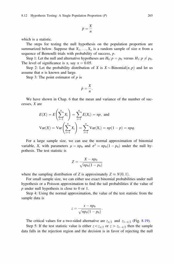
p ¼ Xn
which is a statistic.The steps for testing the null hypothesis on the population proportion are
summarized below. Suppose that X1; . . .;Xn is a random sample of size n from asequence of Bernoulli trials with probability of success, p.
Step 1: Let the null and alternative hypotheses are H0: p ¼ p0 versus H1: p 6¼ p0.The level of significance is a, say a ¼ 0:05.
Step 2: Let the probability distribution of X is X �Binomialðn; pÞ and let usassume that n is known and large.
Step 3: The point estimator of p is
p ¼ Xn:
We have shown in Chap. 6 that the mean and variance of the number of suc-cesses, X are
EðXÞ ¼ EXni¼1
Xi
!¼Xni¼1
EðXiÞ ¼ np; and
VarðXÞ ¼ VarXni¼1
Xi
!¼Xni¼1
VarðXiÞ ¼ npð1� pÞ ¼ npq:
For a large sample size, we can use the normal approximation of binomialvariable, X, with parameters l ¼ np0 and r2 ¼ np0ð1� p0Þ under the null hy-pothesis. The test statistic is
Z ¼ X � np0ffiffiffiffiffiffiffiffiffiffiffiffiffiffiffiffiffiffiffiffiffiffiffinp0ð1� p0Þ
pwhere the sampling distribution of Z is approximately Z � Nð0; 1Þ.
For small sample size, we can either use exact binomial probabilities under nullhypothesis or a Poisson approximation to find the tail probabilities if the value ofp under null hypothesis is close to 0 or 1.
Step 4: Using the normal approximation, the value of the test statistic from thesample data is
z ¼ x� np0ffiffiffiffiffiffiffiffiffiffiffiffiffiffiffiffiffiffiffiffiffiffiffinp0ð1� p0Þ
p :
The critical values for a two-sided alternative are za=2 and z1�a=2 (Fig. 8.19).Step 5: If the test statistic value is either z\za=2 or z[ z1�a=2 then the sample
data falls in the rejection region and the decision is in favor of rejecting the null
8.12 Hypothesis Testing: A Single Population Proportion (P) 265

hypothesis. On the other hand, if za=2\z\z1�a=2 then the test statistic value is inthe non-rejection region and the decision is in favor of non-rejection of nullhypothesis for the given sample data.
Example 8.7 In a study on the diagnosis of acute inflammations of the urinarybladder and acute nephritises, a sample of 120 subjects is considered (Czerniak andZarzycki 2003). The inflammation of urinary bladder is found among 59 out of 120subjects. The hypothesis needs to be tested is whether the true population pro-portion is 50% of the total subjects in the population. The level of significance isa ¼ 0:05.
SolutionThe steps in testing the whether the specified value is the true population proportionare illustrated here.
Step 1: H0: p ¼ 0:5 versus H1: p 6¼ 0:5.The level of significance is a ¼ 0:05.Step 2: X�Binomialðn; pÞ, n is known and large.Step 3: The point estimator of p isp ¼ X
n. The expected value and variance of the estimator are
EðXÞ ¼ np; ðandÞ
VarðXÞ ¼ npð1� pÞ:
The test statistic is approximately normal under null hypothesis with parametersl ¼ np0 and r2 ¼ np0ð1� p0Þ which is
Fig. 8.19 Figure displaying critical regions for test about population proportion assumingnormality approximation
266 8 Hypothesis Testing
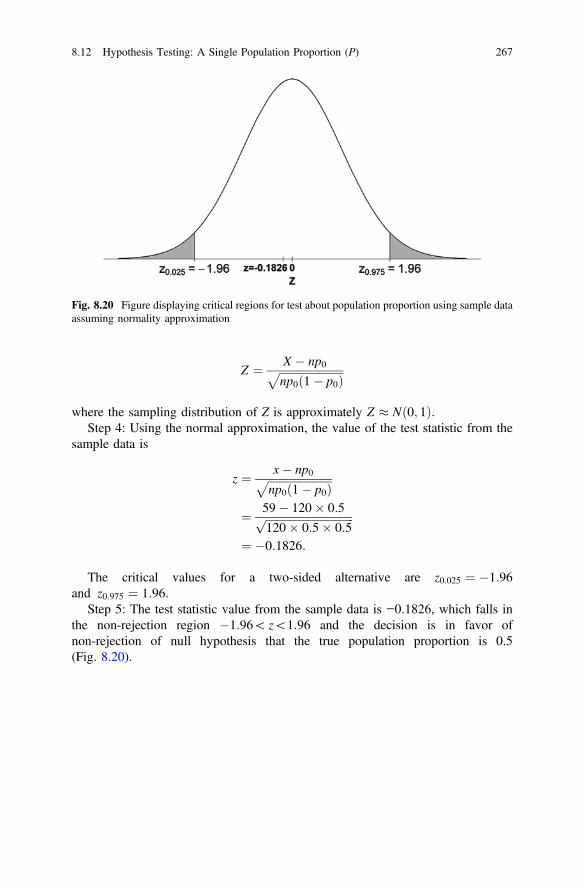
Z ¼ X � np0ffiffiffiffiffiffiffiffiffiffiffiffiffiffiffiffiffiffiffiffiffiffiffinp0ð1� p0Þ
pwhere the sampling distribution of Z is approximately Z � Nð0; 1Þ.
Step 4: Using the normal approximation, the value of the test statistic from thesample data is
z ¼ x� np0ffiffiffiffiffiffiffiffiffiffiffiffiffiffiffiffiffiffiffiffiffiffiffinp0ð1� p0Þ
p¼ 59� 120� 0:5ffiffiffiffiffiffiffiffiffiffiffiffiffiffiffiffiffiffiffiffiffiffiffiffiffiffiffiffiffiffiffiffi
120� 0:5� 0:5p
¼ �0:1826:
The critical values for a two-sided alternative are z0:025 ¼ �1:96and z0:975 ¼ 1:96.
Step 5: The test statistic value from the sample data is −0.1826, which falls inthe non-rejection region �1:96\ z\1:96 and the decision is in favor ofnon-rejection of null hypothesis that the true population proportion is 0.5(Fig. 8.20).
Fig. 8.20 Figure displaying critical regions for test about population proportion using sample dataassuming normality approximation
8.12 Hypothesis Testing: A Single Population Proportion (P) 267

8.13 Hypothesis Testing: The Difference Between TwoPopulation Proportions (P1 − P2)
In this section, we are interested in testing some hypotheses about the differencebetween two population proportions (p1 − p2). Suppose that we have two popula-tions with p1 = population proportion of the first population, p2 = population pro-portion of the second population. We want to compare p1 and p2, or equivalently, tomake inferences about p1 − p2. If we select a random sample of size n1 from the firstBernoulli population with parameter p1 and another random sample of size n2 fromthe second Bernoulli population with parameter p2 then let X1 = number of elementsof type A in the first sample and X2 = number of elements of type A in the secondsample. Then, we can define p1 ¼ X1
n1= the sample proportion of the first sample and
p2 ¼ X2n2
= the sample proportion of the second sample. The sampling distribution ofp1 � p2 is used to make inferences about p1 − p2.
For large n1 and n2, we can show asymptotically
Z ¼ ðp1 � p2Þ � ðp1 � p2Þffiffiffiffiffiffiffiffiffiffiffiffiffiffiffiffiffiffiffiffip1q1n1
þ p2q2n2
q �N 0; 1ð Þ
where q1 ¼ 1� p1 and q2 ¼ 1� p2.The steps for testing the null hypothesis on the equality of population propor-
tions are shown below.Step 1: The null and alternative hypotheses are H0: p1 ¼ p2 versus H1: p1 6¼ p2.
The level of significance is a, say a ¼ 0:05.Step 2: Let the probability distribution of X1 and X2 are X1 �Binomialðn1; p1Þ
and X2 �Binomialðn2; p2Þ respectively.Step 3: The point estimator of p1 and p2 are
p1 ¼ X1
n1
and
p2 ¼ X2
n2:
The mean and variance of the difference between two population proportions,assuming independence of X1 and X2, are
Eðp1 � p2Þ ¼ p1 � p2; and
Varðp1 � p2Þ ¼ p1ð1� p1Þn1
þ p2ð1� p2Þn2
:
268 8 Hypothesis Testing

For large sample sizes n1 and n2, we can use the following test statistic as anapproximation of difference between two binomial proportions with parameters
lp1�p2 ¼ p1 � p2 and r2p1�p2 ¼p1ð1�p1Þ
n1þ p2ð1�p2Þ
n2.
The test statistic is
Z ¼ p1 � p2 � ðp1 � p2Þffiffiffiffiffiffiffiffiffiffiffiffiffiffiffiffiffiffiffiffiffiffiffiffiffiffiffiffiffiffiffiffiffiffip1ð1�p1Þ
n1þ p2ð1�p2Þ
n2
q
and under the null hypothesis of equality of these proportions, the test statisticbecomes
Z ¼ p1 � p2ffiffiffiffiffiffiffiffiffiffiffiffiffiffiffiffiffiffiffiffiffiffiffiffiffiffiffiffiffiffiffiffiffiffip1ð1�p1Þ
n1þ p2ð1�p2Þ
n2
q
where the sampling distribution of Z is approximately Z � Nð0; 1Þ.Step 4: Using the normal approximation, the value of the test statistic from the
sample data is
z ¼ p1 � p2ffiffiffiffiffiffiffiffiffiffiffiffiffiffiffiffiffiffiffiffiffiffiffiffiffiffiffiffiffiffiffiffiffiffip1ð1�p1Þ
n1þ p2ð1�p2Þ
n2
q :
However, under the null hypothesis p1 ¼ p2, hence, a pooled estimator of p canbe computed
p ¼ x1 þ x2n1 þ n2
:
Then, z can be redefined as
z ¼ p1 � p2ffiffiffiffiffiffiffiffiffiffiffiffiffiffiffiffiffiffiffiffiffiffiffiffiffiffiffiffiffiffiffiffiffiffiffipð1� pÞ 1
n1þ 1
n2
h ir :
We can find the critical values for a two-sided alternative, za=2 and z1�a=2
(Fig. 8.21).Step 5: If the test statistic value is either z\za=2 or z[ z1�a=2 then the sample
data favor rejection of the null hypothesis that there is equality of populationproportions. On the other hand, if za=2\z\z1�a=2 then the test statistic value is inthe non-rejection region and the decision is in favor of non-rejection of nullhypothesis for the sample data.
Example 8.8 In Chap. 7, we have shown an example of constructing confidenceinterval of difference between two proportions. The same hypothetical data are
8.13 Hypothesis Testing: The Difference Between Two Population … 269

employed in this chapter to illustrate the procedure for testing the hypothesis ofequality of two population proportions. Let us consider that a researcher has con-ducted a study to compare the proportion of people suffering from breathingproblem in two cities, A and B. In a random sample of 2500 people from city A,110 are suffering from breathing problem and in another independent randomsample of 2000 people, 74 people from city B are found to have breathing problem.The researcher wants to test for equality of proportions of people suffering frombreathing problem in cities A and B. The level of significance is 0.05.
SolutionThe steps for conducting the test hypothesis for the example are illustrated below.
Step 1: H0: p1 ¼ p2 versus H1: p1 6¼ p2.The level of significance is a, say a ¼ 0:05.Step 2: The independent probability distributions for number of people suffering
from breathing problem in cities A and B, respectively, areX1 �Binomialðn1; p1Þ for city A and X2 �Binomialðn2; p2Þ for city B.Step 3: The point estimator of p1 and p2 are
p1 ¼ X1
n1
and
p2 ¼ X2
n2:
Fig. 8.21 Figure displaying critical regions for test about equality of population proportionsassuming normality approximation
270 8 Hypothesis Testing

Assuming independence of X1 and X2, the mean and variance of the differencebetween two population proportions are
Eðp1 � p2Þ ¼ p1 � p2; and Varðp1 � p2Þ ¼ p1ð1� p1Þn1
þ p2ð1� p2Þn2
:
For large sample size, the test statistic under null hypothesis is
Z ¼ p1 � p2ffiffiffiffiffiffiffiffiffiffiffiffiffiffiffiffiffiffiffiffiffiffiffiffiffiffiffiffiffiffiffiffiffiffip1ð1�p1Þ
n1þ p1ð1�p1Þ
n1
q
where the sampling distribution of Z can be shown approximately as Z � Nð0; 1Þ.Step 4: The estimates of p1 and p2 as well as the pooled estimator of p can be
computed
p1 ¼ x1n1
¼ 1102500
¼ 0:044;
p2 ¼ x2n2
¼ 742000
¼ 0:037;
and
p ¼ x1 þ x2n1 þ n2
:
¼ 110þ 742500þ 2000
¼ 0:041:
Then z can be obtained as
z ¼ p1 � p2ffiffiffiffiffiffiffiffiffiffiffiffiffiffiffiffiffiffiffiffiffiffiffiffiffiffiffiffiffiffiffiffiffiffiffipð1� pÞ 1
n1þ 1
n2
h ir
¼ 0:044� 0:037ffiffiffiffiffiffiffiffiffiffiffiffiffiffiffiffiffiffiffiffiffiffiffiffiffiffiffiffiffiffiffiffiffiffiffiffiffiffiffiffiffiffiffiffiffiffiffiffiffiffiffiffi0:041� 0:959 1
2500 þ 12000
� �q¼ 1:1771:
We can find the critical values for a two-sided alterna-tive,z0:025 ¼ �1:96 and z0:975 ¼ 1:96 (Fig. 8.22).
Step 5: The test statistic value falls in the non-rejection region, �196\z\1:96,so the decision is made in favor of non-rejection of the null hypothesis that theproportion of population with breathing problem is the same in cities A and B.
8.13 Hypothesis Testing: The Difference Between Two Population … 271

8.14 Summary
The concepts and techniques of hypothesis testing are introduced in this chapter.The definition and concept of null and alternative hypotheses, rejection andnon-rejection of null hypothesis, one-sided and two-sided tests, test statistic, typesof error, critical region, and p-value are discussed with examples. The step-by-stepprocedures of testing a null hypothesis against an alternative are shown in thischapter. The hypothesis testing procedures are illustrated with examples for singlemean and single proportion and difference between two means and two proportionsunder various situations arising from assumptions about population (normal ornon-normal), sample size (small or large), population variance (known orunknown), and sample sizes equal or unequal in case of two samples. In addition, ifthe equality of population means is tested for correlated data then the paired t-test isshown with an example. This chapter includes many examples to illustrate theprocedures in easy steps.
Exercises
8:1 Explain the following briefly with example:
(i) Null and alternative hypotheses,(ii) Non-rejection and rejection of null hypothesis,(iii) One-sided and two-sided tests,(iv) Test statistic,(v) Type I and Type II errors,(vi) Level of significance,(vii) Critical region, and(viii) P-value.
Fig. 8.22 Figure displaying critical regions for test about equality of population proportions usingsample data assuming normality approximation
272 8 Hypothesis Testing
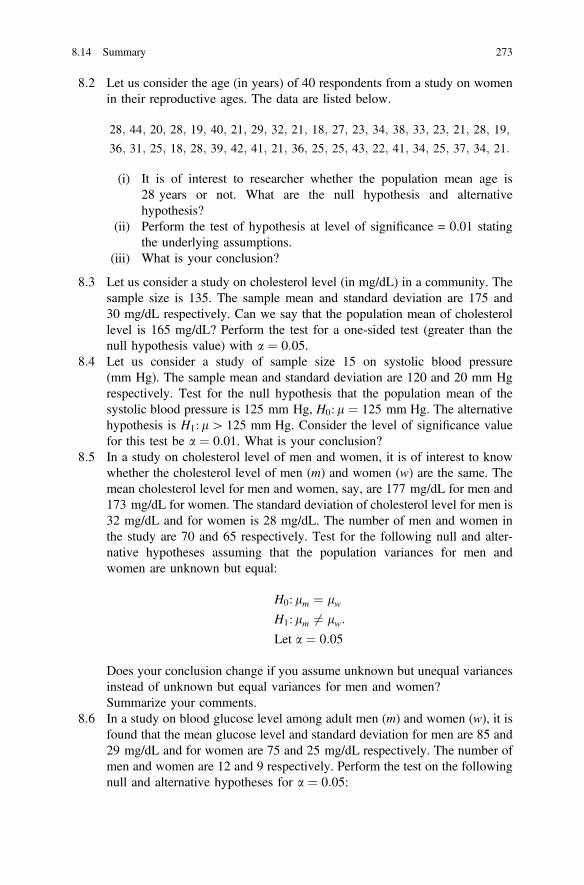
8:2 Let us consider the age (in years) of 40 respondents from a study on womenin their reproductive ages. The data are listed below.
28; 44; 20; 28; 19; 40; 21; 29; 32; 21; 18; 27; 23; 34; 38; 33; 23; 21; 28; 19;
36; 31; 25; 18; 28; 39; 42; 41; 21; 36; 25; 25; 43; 22; 41; 34; 25; 37; 34; 21:
(i) It is of interest to researcher whether the population mean age is28 years or not. What are the null hypothesis and alternativehypothesis?
(ii) Perform the test of hypothesis at level of significance = 0.01 statingthe underlying assumptions.
(iii) What is your conclusion?
8:3 Let us consider a study on cholesterol level (in mg/dL) in a community. Thesample size is 135. The sample mean and standard deviation are 175 and30 mg/dL respectively. Can we say that the population mean of cholesterollevel is 165 mg/dL? Perform the test for a one-sided test (greater than thenull hypothesis value) with a ¼ 0:05.
8:4 Let us consider a study of sample size 15 on systolic blood pressure(mm Hg). The sample mean and standard deviation are 120 and 20 mm Hgrespectively. Test for the null hypothesis that the population mean of thesystolic blood pressure is 125 mm Hg, H0: l ¼ 125 mm Hg. The alternativehypothesis is H1: l[ 125 mm Hg. Consider the level of significance valuefor this test be a ¼ 0:01. What is your conclusion?
8:5 In a study on cholesterol level of men and women, it is of interest to knowwhether the cholesterol level of men (m) and women (w) are the same. Themean cholesterol level for men and women, say, are 177 mg/dL for men and173 mg/dL for women. The standard deviation of cholesterol level for men is32 mg/dL and for women is 28 mg/dL. The number of men and women inthe study are 70 and 65 respectively. Test for the following null and alter-native hypotheses assuming that the population variances for men andwomen are unknown but equal:
H0: lm ¼ lwH1: lm 6¼ lw:
Let a ¼ 0:05
Does your conclusion change if you assume unknown but unequal variancesinstead of unknown but equal variances for men and women?Summarize your comments.
8:6 In a study on blood glucose level among adult men (m) and women (w), it isfound that the mean glucose level and standard deviation for men are 85 and29 mg/dL and for women are 75 and 25 mg/dL respectively. The number ofmen and women are 12 and 9 respectively. Perform the test on the followingnull and alternative hypotheses for a ¼ 0:05:
8.14 Summary 273

H0: lm ¼ lw:
H1: lm [ lw:
Comment on your test results.8:7 An experiment was conducted to compare time duration of stay in a hospital
with two types of complications (A) and (B) and 9 patients with complicationtype A and 16 patients with complication type B were selected randomly.The average time lengths were 12 days for A and 7 days for B and samplevariances were 8 days2 for A and 5 days2 for B. Assuming equality ofvariances in the populations, test for the equality of population means at 1%level of significance.
8:8 Let the proportion of obese children estimated from a sample of size 100 is0.15. Test for the following null and alternative hypotheses at 5% level ofsignificance and comment on your findings:
H0: p ¼ 0:20:
H1: p 6¼ 0:20:
8:9 Among the adult males and females, a study is conducted to estimate theproportion of diabetics. The sample sizes are 250 for males and 200 forfemales. It is found from the estimates from the samples that the proportionof diabetics among males is 10% and among females is 7%. Test for theequality of proportions of diabetics among males and females in the popu-lation at 5% level of significance. Consider the one-sided alternative that theproportion of diabetics is higher among the males.
8:10 Following results are given from two independent random samples:p1 ¼ 0:3; n1 ¼ 49, and p2 ¼ 0:5; n2 ¼ 81. Test for the equality of twopopulation proportions and then comment on the test result.
8:11 Following results are given from two independent random samples:�x1 ¼ 20; s21 ¼ 16; n1 ¼ 10, and �x2 ¼ 25; s22 ¼ 16; n2 ¼ 12. State the null andalternative hypotheses for testing the equality of two population means andcomment on the result, if r21 and r22 are unknown and assumed to be equal.
8:12 The following hypothetical data show the systolic blood pressure (SBP) of10 subjects before and after exercise:
SBP before exercise (mm Hg) SBP after exercise (mm Hg)
115 125
120 132
100 114
125 130
121 130
117 132
106 119(continued)
274 8 Hypothesis Testing

(continued)
SBP before exercise (mm Hg) SBP after exercise (mm Hg)
118 131
110 121
117 128
Perform the test for the null hypothesis that there is no difference in the mean ofsystolic blood pressure due to exercise. What would be a reasonable alternativehypothesis? Justify your choice of the alternative hypothesis. Comment on your testresult. The level of significance is 0.05.
References
Czerniak, J., & Zarzycki, H. (2003). Application of rough sets in the presumptive diagnosis ofurinary system diseases, Artificial Intelligence and Security in Computing Systems. ACCS2002 9th International Conference Proceedings (pp. 41–51). Kluwer Academic Publishers.
Goodman, S. N. (1992). A comment on replication. P-values and evidence. Statistics in Medicine,11(7), 875–879.
Hung, H. M., O’Neill, R. T., Bauer, P., & Kohne, K. (1997). The behavior of the P-value when thealternative hypothesis is true. Biometrics, 53(1), 11–22.
Satterthwaite, F. E. (1946). An approximate distribution of variance components. BiometricsBulletin, 2(6), 110–114.
Wasserstein, R. L., & Lazar, N. A. (2016). The ASA’s statement on p-values: Context, process,and purpose. The American Statistician, 70(2), 129–133. https://doi.org/10.1080/00031305.2016.1154108.
8.14 Summary 275

Chapter 9Correlation and Regression
9.1 Introduction
In many applications, we may want to study the underlying nature of relationshipsamong the variables. Furthermore, we may also want to utilize these relationshipsfor predicting or estimating the values of some variables (outcome variables) on thebasis of the given values of other variables (explanatory variables). By exploringthe underlying relationships, we can find whether there is any association betweenvariables as well as whether there is dependence of outcome variables onexplanatory variables that can provide necessary inputs required for useful deci-sions. Some examples of these relationships are (i) relationship between height andweight, (ii) relationship between weight and cholesterol level, (iii) relationshipbetween income and expenditure on health care, etc. In these studies, we areinterested in answering several important questions, some of which are
(i) Is there a relationship between the variables? What is the nature of this rela-tionship? What is the strength of this relationship?
(ii) If there is a relationship between the variables, how can we formulate itmathematically? How can we interpret it? What are the policy implications?What is the significance of such finding in explaining the underlying truth inpopulation?
Suppose that we are interested in studying the relationship between the height ofthe person and his weight in a certain population of a community. In this case, weselect a random sample of size n from this population, and then we measure theheight (X) and the weight (Y) of each individual in the sample. The random sampleof pairs of variables is
ðX1; Y1Þ; ðX2; Y2Þ; . . .; ðXn; YnÞ:
The observations of the sample will be a set of pairs ðx1; y1Þ; ðx2; y2Þ; . . .; ðxn; ynÞ
© Springer Nature Singapore Pte Ltd. 2018M. A. Islam and A. Al-Shiha, Foundations of Biostatistics,https://doi.org/10.1007/978-981-10-8627-4_9
277
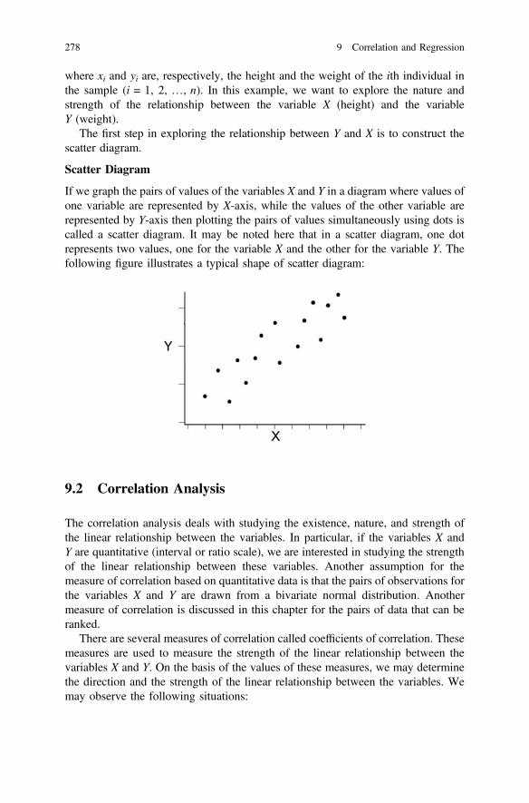
where xi and yi are, respectively, the height and the weight of the ith individual inthe sample (i = 1, 2, …, n). In this example, we want to explore the nature andstrength of the relationship between the variable X (height) and the variableY (weight).
The first step in exploring the relationship between Y and X is to construct thescatter diagram.
Scatter Diagram
If we graph the pairs of values of the variables X and Y in a diagram where values ofone variable are represented by X-axis, while the values of the other variable arerepresented by Y-axis then plotting the pairs of values simultaneously using dots iscalled a scatter diagram. It may be noted here that in a scatter diagram, one dotrepresents two values, one for the variable X and the other for the variable Y. Thefollowing figure illustrates a typical shape of scatter diagram:
9.2 Correlation Analysis
The correlation analysis deals with studying the existence, nature, and strength ofthe linear relationship between the variables. In particular, if the variables X andY are quantitative (interval or ratio scale), we are interested in studying the strengthof the linear relationship between these variables. Another assumption for themeasure of correlation based on quantitative data is that the pairs of observations forthe variables X and Y are drawn from a bivariate normal distribution. Anothermeasure of correlation is discussed in this chapter for the pairs of data that can beranked.
There are several measures of correlation called coefficients of correlation. Thesemeasures are used to measure the strength of the linear relationship between thevariables X and Y. On the basis of the values of these measures, we may determinethe direction and the strength of the linear relationship between the variables. Wemay observe the following situations:
278 9 Correlation and Regression

(i) The coefficient of correlation is positive if the large values of Y are associatedwith large values of X which implies that the values of Y tend to be large withlarge values of X, and vice versa.
(ii) The coefficient of correlation is negative if the large values of Y are asso-ciated with small values of X implying that the values of Y tend to be largewith small values of X, and vice versa.
(iii) The coefficient of correlation is zero if the values of Y are not linearlyaffected by the values of X.
It may also be noted here that the existence of correlation indicating a linearassociation between variables does not necessarily imply that there is a cause andeffect relationship between the variables.
The following figures illustrate some typical cases.
(a) Complete (perfect) negative linear
correlation
(b) Complete (perfect) positive linear
correlation
(c) Negative linear correlation (d) Positive linear correlation
9.2 Correlation Analysis 279

(e) No linear correlation (f) No linear correlation
(g) Strong positive linear correlation
(scatter points are more clustered
around a line)
(h) Weak positive linear correlation
(scatter points are less clustered around
a line)
There are several measures used to measure the correlation or associationbetween variables. Two of these measures commonly employed are
(i) Pearson’s correlation coefficient: This measure is used in the case where bothvariables are quantitative.
(ii) Spearman’s Rank Correlation coefficient: This measure is used in the casewhere the variables can be expressed as ranks.
9.2.1 Pearson’s Correlation Coefficient
The Pearson’s correlation coefficient provides a measure of the strength of linearrelationship between two variables, say X and Y. As we have mentioned earlier, thismeasure can be used when both variables are ratio or interval scaled.
280 9 Correlation and Regression

Definition
The population correlation coefficient for N pairs of population valuesðX1; Y1Þ; ðX2; Y2Þ; . . .; ðXN ; YNÞ is defined by
q ¼PN
i¼1 ðXi � lXÞðYi � lYÞffiffiffiffiffiffiffiffiffiffiffiffiffiffiffiffiffiffiffiffiffiffiffiffiffiffiffiffiffiffiffiffiffiffiffiffiffiffiPNi¼1 ðXi � lXÞ2=N
q ffiffiffiffiffiffiffiffiffiffiffiffiffiffiffiffiffiffiffiffiffiffiffiffiffiffiffiffiffiffiffiffiffiffiffiffiffiffiPNi¼1 ðYi � lYÞ2=N
q¼ E X � lXð Þ Y � lYð Þ½ �ffiffiffiffiffiffiffiffiffiffiffiffiffiffiffiffiffiffiffiffiffiffiffi
EðX � lXÞ2q ffiffiffiffiffiffiffiffiffiffiffiffiffiffiffiffiffiffiffiffiffiffiffi
EðY � lYÞ2q
¼ rXYffiffiffiffiffiffir2X
p ffiffiffiffiffiffir2Y
p;
where lX ¼PNi¼1 Xi=N; lY ¼PN
i¼1 Yi=N; rXY ¼PNi¼1 ðXi � lXÞðYi � lYÞ=N;
r2X ¼PNi¼1ðXi � lXÞ2 and r2Y ¼PN
i¼1ðYi � lYÞ2:As we cannot measure the population correlation coefficient generally due to
lack of observing the pairs of values from the population, we estimate it by thesample correlation coefficient.
The sample correlation coefficient for n given pairs of observationsðx1; y1Þ; . . .; ðxn; ynÞ is denoted by r and is defined by
r ¼Pn
i¼1 ðxi � xÞðyi � �yÞ=nffiffiffiffiffiffiffiffiffiffiffiffiffiffiffiffiffiffiffiffiffiffiffiffiffiffiffiffiffiffiffiffiffiPni¼1 ðxi � xÞ2=n
q ffiffiffiffiffiffiffiffiffiffiffiffiffiffiffiffiffiffiffiffiffiffiffiffiffiffiffiffiffiffiffiffiffiPni¼1 ðyi � �yÞ2=n
q¼
Pni¼1 ðxi � xÞðyi � �yÞffiffiffiffiffiffiffiffiffiffiffiffiffiffiffiffiffiffiffiffiffiffiffiffiffiffiffiffiffiPn
i¼1 ðxi � xÞ2q ffiffiffiffiffiffiffiffiffiffiffiffiffiffiffiffiffiffiffiffiffiffiffiffiffiffiffiffiffiPn
i¼1 ðyi � �yÞ2q
¼ SxyffiffiffiffiffiffiSxx
p ffiffiffiffiffiffiSyy
p ;
where Sxy ¼Pn
i¼1 ðxi � �xÞðyi � �yÞ, Sxx ¼Pn
i¼1 ðxi � �xÞ2, and Syy ¼Pn
i¼1 ðyi � �yÞ2.The computational formula for calculating r is shown below
r ¼Pn
i¼1 xiyi � n�x�yffiffiffiffiffiffiffiffiffiffiffiffiffiffiffiffiffiffiffiffiffiffiffiffiffiffiffiffiffiffiffiffiPni¼1 x
2i � nð�xÞ2
q ffiffiffiffiffiffiffiffiffiffiffiffiffiffiffiffiffiffiffiffiffiffiffiffiffiffiffiffiffiffiffiffiPni¼1 y
2i � nð�yÞ2
qwhich can be expressed in the following form too:
r ¼ nPn
i¼1 xiyi �Pn
i¼1 xiPn
i¼1 yiffiffiffiffiffiffiffiffiffiffiffiffiffiffiffiffiffiffiffiffiffiffiffiffiffiffiffiffiffiffiffiffiffiffiffiffiffiffiffiffiffiffiffiffiffiffinPn
i¼1 x2i �
Pni¼1 xi
� �2q ffiffiffiffiffiffiffiffiffiffiffiffiffiffiffiffiffiffiffiffiffiffiffiffiffiffiffiffiffiffiffiffiffiffiffiffiffiffiffiffiffiffiffiffiffiffinPn
i¼1 y2i �
Pni¼1 yi
� �2q :
9.2 Correlation Analysis 281
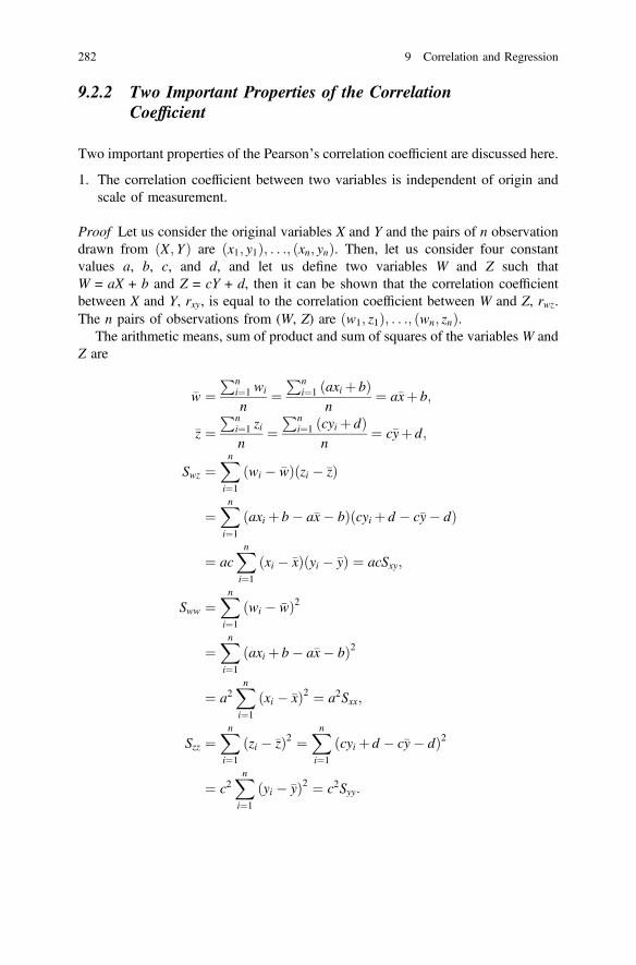
9.2.2 Two Important Properties of the CorrelationCoefficient
Two important properties of the Pearson’s correlation coefficient are discussed here.
1. The correlation coefficient between two variables is independent of origin andscale of measurement.
Proof Let us consider the original variables X and Y and the pairs of n observationdrawn from ðX; YÞ are ðx1; y1Þ; . . .; ðxn; ynÞ. Then, let us consider four constantvalues a, b, c, and d, and let us define two variables W and Z such thatW = aX + b and Z = cY + d, then it can be shown that the correlation coefficientbetween X and Y, rxy, is equal to the correlation coefficient between W and Z, rwz.The n pairs of observations from (W, Z) are ðw1; z1Þ; . . .; ðwn; znÞ.
The arithmetic means, sum of product and sum of squares of the variables W andZ are
�w ¼Pn
i¼1 wi
n¼Pn
i¼1 ðaxi þ bÞn
¼ a�xþ b;
�z ¼Pn
i¼1 zin
¼Pn
i¼1 ðcyi þ dÞn
¼ c�yþ d;
Swz ¼Xni¼1
ðwi � �wÞðzi � �zÞ
¼Xni¼1
ðaxi þ b� a�x� bÞðcyi þ d � c�y� dÞ
¼ acXni¼1
ðxi � �xÞðyi � �yÞ ¼ acSxy;
Sww ¼Xni¼1
ðwi � �wÞ2
¼Xni¼1
ðaxi þ b� a�x� bÞ2
¼ a2Xni¼1
ðxi � �xÞ2 ¼ a2Sxx;
Szz ¼Xni¼1
ðzi � �zÞ2 ¼Xni¼1
ðcyi þ d � c�y� dÞ2
¼ c2Xni¼1
ðyi � �yÞ2 ¼ c2Syy:
282 9 Correlation and Regression

The correlation coefficient between W and Z is
rwz ¼Pn
i¼1 ðwi � �wÞðzi � �zÞffiffiffiffiffiffiffiffiffiffiffiffiffiffiffiffiffiffiffiffiffiffiffiffiffiPni¼1
ðwi � �wÞ2s ffiffiffiffiffiffiffiffiffiffiffiffiffiffiffiffiffiffiffiffiffiffiffiPn
i¼1ðzi � �zÞ2
s
¼ SwzffiffiffiffiffiffiffiffiSww
p ffiffiffiffiffiffiSzz
p ¼ acSxyffiffiffiffiffiffiffiffiffiffia2Sxx
p ffiffiffiffiffiffiffiffiffiffic2Syy
p¼ Sxyffiffiffiffiffiffi
Sxxp ffiffiffiffiffiffi
Syyp ¼ rxy:
The above result proves that the correlation coefficient between two variables isindependent of origin and scale of measurement.
2. The value of the correlation coefficient lies between −1 and +1.
Proof As we know that the correlation coefficient is independent of origin andscale, let us assume that �x ¼ �y ¼ 0. Let us consider the following nonnegativeexpression:
Q ¼Xni¼1
ðaxi � yÞ2;
where a is any constant value.Then, we can show that
Q ¼Xni¼1
ðaxi � yÞ2 ¼Xni¼1
ða2x2i � 2axiyi þ y2i Þ� 0
which is
a2Xni¼1
x2i � 2aXni¼1
xiyi þXni¼1
y2i � 0
!
As the above inequalities hold for any value of a, let us put a ¼Pn
i¼1xiyiPn
i¼1x2i, then,
the above inequality can be expressed asPni¼1 xiyiPni¼1 x
2i
� �2Xn
i¼1x2i � 2
Pni¼1 xiyiPni¼1 x
2i
� �Xn
i¼1xiyi þ
Xn
i¼1y2i � 0
9.2 Correlation Analysis 283
and Pni¼1 xiyi
� �2Pni¼1 x
2i
� 2Pn
i¼1 xiyi� �2Pn
i¼1 x2i
þXni¼1
y2i � 0:
Multiplying both sides byPn
i¼1 x2i , we have
�Xni¼1
xiyi
!2
þXni¼1
x2i
! Xni¼1
y2i
!� 0
which can be expressed as
Xni¼1
x2i
! Xni¼1
y2i
!�
Xni¼1
xiyi
!2
and dividing both sides byPn
i¼1 x2i
� � Pni¼1 y
2i
� �1�
Pni¼1 xiyi
� �2Pni¼1 x
2i
� � Pni¼1 y
2i
� � ¼ r2:
It means that
r2 � 1
which proves �1� r� 1:Some important points to be remembered about the correlation coefficient are
listed below.
1. The value of r lies between −1 and +1, inclusive, that is −1� r � +1.2. If the correlation (linear association) is positive and strong, then the value of r is
close to +1.3. If the correlation (linear association) is negative and strong, then the value of r is
close to −1.4. If the correlation (linear association) is weak, then the value of r is close to 0.5. If there is no correlation (no linear association) between the variables, i.e., if
there is no linear relationship between the variables, then the value of r equals 0.However, this does not mean that there is no other form of nonlinear relationshipbetween the variables.
6. A positive correlation with value (r = +a) and a negative correlation with value(r =−a) (where 0 < a � 1) have the same strength and opposite directions.
7. The existence of correlation (linear association) between variables, even if it isstrong, does not imply that there is a cause and effect relationship between them.For instance, a strong positive correlation between income and saving does notmean that more income causes more saving.
284 9 Correlation and Regression
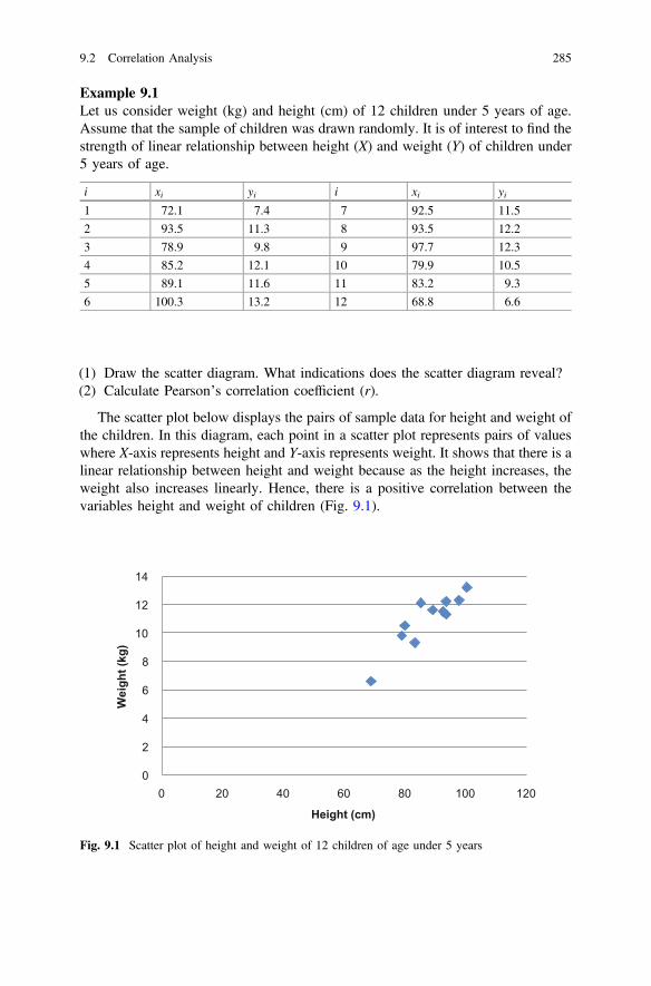
Example 9.1Let us consider weight (kg) and height (cm) of 12 children under 5 years of age.Assume that the sample of children was drawn randomly. It is of interest to find thestrength of linear relationship between height (X) and weight (Y) of children under5 years of age.
i xi yi i xi yi1 72.1 7.4 7 92.5 11.5
2 93.5 11.3 8 93.5 12.2
3 78.9 9.8 9 97.7 12.3
4 85.2 12.1 10 79.9 10.5
5 89.1 11.6 11 83.2 9.3
6 100.3 13.2 12 68.8 6.6
(1) Draw the scatter diagram. What indications does the scatter diagram reveal?(2) Calculate Pearson’s correlation coefficient (r).
The scatter plot below displays the pairs of sample data for height and weight ofthe children. In this diagram, each point in a scatter plot represents pairs of valueswhere X-axis represents height and Y-axis represents weight. It shows that there is alinear relationship between height and weight because as the height increases, theweight also increases linearly. Hence, there is a positive correlation between thevariables height and weight of children (Fig. 9.1).
0
2
4
6
8
10
12
14
0 20 40 60 80 100 120
Wei
ght (
kg)
Height (cm)
Fig. 9.1 Scatter plot of height and weight of 12 children of age under 5 years
9.2 Correlation Analysis 285

(2) The computation of Pearson’s correlation coefficient is illustrated below for theheight and weight data of 12 children. We have shown that the Pearson’scorrelation coefficient can be computed using the following formula
r ¼Pn
i¼1 xiyi � n�x�yffiffiffiffiffiffiffiffiffiffiffiffiffiffiffiffiffiffiffiffiffiffiffiffiffiffiffiffiffiffiffiffiPni¼1 x
2i � nð�xÞ2
q ffiffiffiffiffiffiffiffiffiffiffiffiffiffiffiffiffiffiffiffiffiffiffiffiffiffiffiffiffiffiffiffiPni¼1 y
2i � nð�yÞ2
q :
Table 9.1 can be used to facilitate the computation of the correlation coefficientfrom the sample data.
�x ¼P12
i¼1 xi12
¼ 1034:712
¼ 86:225
�y ¼P12
i¼1 yi12
¼ 127:812
¼ 10:65
The correlation coefficient then can be estimated as
r ¼Pn
i¼1 xiyi � n�x�yffiffiffiffiffiffiffiffiffiffiffiffiffiffiffiffiffiffiffiffiffiffiffiffiffiffiffiffiffiffiffiffiPni¼1 x
2i � nð�xÞ2
q ffiffiffiffiffiffiffiffiffiffiffiffiffiffiffiffiffiffiffiffiffiffiffiffiffiffiffiffiffiffiffiffiPni¼1 y
2i � nð�yÞ2
q¼ 11224:7� 12� 86:225� 10:65ffiffiffiffiffiffiffiffiffiffiffiffiffiffiffiffiffiffiffiffiffiffiffiffiffiffiffiffiffiffiffiffiffiffiffiffiffiffiffiffiffiffiffiffiffiffiffiffiffiffiffiffiffiffi
90307:29� 12� ð86:225Þ2q ffiffiffiffiffiffiffiffiffiffiffiffiffiffiffiffiffiffiffiffiffiffiffiffiffiffiffiffiffiffiffiffiffiffiffiffiffiffiffiffiffiffiffiffiffiffiffiffiffi
1406:38� 12� ð10:65Þ2q
¼ 0:92:
Table 9.1 Table for computation of Pearson’s correlation coefficient on height and weight of 12children under 5 years of age
xHeight (cm)
yWeight (kg)
xy x2 y2
72.1 7.4 533.54 5198.41 54.76
93.5 11.3 1056.55 8742.25 127.69
78.9 9.8 773.22 6225.21 96.04
85.2 12.1 1030.92 7259.04 146.41
89.1 11.6 1033.56 7938.81 134.56
100.3 13.2 1323.96 10060.09 174.24
92.5 11.5 1063.75 8556.25 132.25
93.5 12.2 1140.70 8742.25 148.84
97.7 12.3 1201.71 9545.29 151.29
79.9 10.5 838.95 6384.01 110.25
83.2 9.3 773.76 6922.24 86.49
68.8 6.6 454.08 4733.44 43.56Pxi ¼ 1034:7
Pyi ¼ 127:8
Pxiyi ¼ 11224:7
Px2i ¼ 90307:29
Py2i ¼ 1406:38
286 9 Correlation and Regression

The measure of correlation coefficient shows that: (i) there is a positive linearrelationship between height and weight of children under 5 years of age, and (ii) thelinear relationship between height and weight of children appears to be quite strong.
9.2.3 Inferences About the Correlation Coefficient
In the previous section, we have seen that the first step in studying the relationshipbetween two quantitative phenomena are construction of the scatter diagram andcalculating the value of the correlation coefficient using Pearson’s correlationcoefficient, r. Indeed, the calculated value of r is used as a point estimate for the truevalue of the coefficient of linear correlation between X and Y, denoted by q.
The second step is to test the significance of the true value of (q) and con-structing confidence intervals about it.
(i) Testing hypotheses about the coefficient of linear correlation (q)
Suppose that ðX1; Y1Þ; ðX2; Y2Þ. . .; ðXn; YnÞ is a random sample of size n takenfrom a bivariate normal distribution with linear correlation coefficient q.
We are interested in knowing whether there is a correlation between the vari-ables X and Y (q 6¼ 0) or not (q ¼ 0). Also, we are interested in knowing the natureof the linear correlation in case it exists; whether it is positive (q[ 0) or negative(q\0). In other words, we aew interested in testing hypotheses according to one ofthe following cases:
(a)H0: q ¼ 0H1: q 6¼ 0
�(b)
H0: q� 0H1: q[ 0
�(c)
H0: q� 0H1: q\0
�
The test statistic for testing these hypotheses for r from the pairs of randomsample data ðX1; Y1Þ; . . .; ðXn; YnÞ is
T ¼ rffiffiffiffiffiffiffiffiffiffiffin� 2
pffiffiffiffiffiffiffiffiffiffiffiffiffi1� r2
p
where r is the estimator of the Pearson’s coefficient of correlation. UnderH0: q ¼ 0, the test statistic T has a t-distribution with degrees offreedom = m ¼ n� 2.
The test statistic value of T from observed sample data ðx1; y1Þ; . . .; ðxn; ynÞ is
t ¼ rffiffiffiffiffiffiffiffiffiffiffin� 2
pffiffiffiffiffiffiffiffiffiffiffiffiffi1� r2
p
where r is computed from the sample data. The decision of rejecting or not rejectingH0: q ¼ 0 will be as follows according to the three cases mentioned above:
9.2 Correlation Analysis 287

(a) For the first case: We reject H0: q ¼ 0 against H1: q 6¼ 0 at the level of sig-nificance a if t[ tðn�2Þ;1�a=2 or if t\� tðn�2Þ;1�a=2. That is we reject H0: q ¼ 0if jtj[ tðn�2Þ;a=2.
(b) For the second case: We reject H0: q� 0 against H1: q[ 0 at the level ofsignificance a if t[ tðn�2Þ;1�a.
(c) For the third case: We reject H0: q� 0 against H1: q\0 at the level of sig-nificance a if t\� tðn�2Þ;1�a.
288 9 Correlation and Regression

A more general approach of testing the null hypothesis H0: q ¼ q0 against one-or two-sided alternatives is based on Fisher’s transformation of r which tends tonormal distribution with an increase in the sample size. The Fisher’s transformationof r is
Z ¼ 12ln
1þ r1� r
� �and VarðZÞ ¼ 1
n�3.
Here, Z is approximately normally distributed with an expected value 12 ln
1þq1�q
� and variance 1
n�3.The test statistic value of Z for the sample data is
z ¼12 ln
1þ r1�r
�� 12 ln
1þ q01�q0
h iffiffiffiffiffiffi1
n�3
q :
Confidence intervals for the coefficient of correlation (q) is obtained from theFisher’s transformation shown above and the confidence interval for q are com-puted from the following:
z� z1�a=2
ffiffiffiffiffiffiffiffiffiffiffi1
n� 3
rwhere let us denote
zL ¼ z� z1�a=2
ffiffiffiffiffiffiffiffiffiffiffi1
n� 3
r;
and
zU ¼ zþ z1�a=2
ffiffiffiffiffiffiffiffiffiffiffi1
n� 3
r:
Using inverse Fisher’s transformation, we can find
z ¼ 12ln
1þ r1� r
� �
9.2 Correlation Analysis 289

which can be expressed as
ln1þ r1� r
� �¼ 2z
) 1þ r1� r
¼ e2z
) 1þ r ¼ ð1� rÞe2z) r e2z þ 1
� � ¼ e2z � 1
) r ¼ e2z � 1e2z þ 1
:
The lower and upper limits of the confidence interval
rL ¼ e2zL � 1e2zL þ 1
;
and
rU ¼ e2zU � 1e2zU þ 1
:
A ð1� aÞ100% confidence interval for q is:
e2zL � 1e2zL þ 1
\q\e2zU � 1e2zU þ 1
:
Example 9.2Using the data displayed in Example 9.1, answer the following questions.
(1) Find a point estimate for the correlation coefficient between X and Y.(2) Find a 95% confidence interval for the correlation coefficient between X and Y.(3) Do the data provide us with a sufficient evidence to conclude that there is a
linear relationship between X and Y? Suppose a ¼ 0:05:
SolutionIn the previous example, we found that the value of the Pearson’s correlationcoefficient is r = 0.92.
(1) A point estimate for the correlation coefficient between X and Y is
r ¼ þ 0:92
(2) In ordered to calculate a 95% confidence interval for the correlation coefficientbetween X and Y, we calculate the following quantities:
290 9 Correlation and Regression
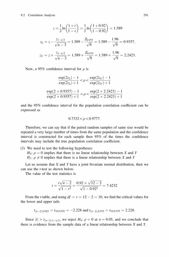
z ¼ 12ln
1þ r1� r
� �¼ 1
2ln
1þ 0:921� 0:92
� �¼ 1:589
zL ¼ z� z1�a=2ffiffiffiffiffiffiffiffiffiffiffin� 3
p ¼ 1:589� Z0:975ffiffiffi9
p ¼ 1:589� 1:96ffiffiffi9
p ¼ 0:9357;
zU ¼ zþ z1�a=2ffiffiffiffiffiffiffiffiffiffiffin� 3
p ¼ 1:589þ Z0:975ffiffiffi9
p ¼ 1:589þ 1:96ffiffiffi9
p ¼ 2:2423:
Now, a 95% confidence interval for q is
expð2zLÞ � 1expð2zLÞþ 1
\q\expð2zUÞ � 1expð2zUÞþ 1
expð2� 0:9357Þ � 1expð2� 0:9357Þþ 1
\q\expð2� 2:2423Þ � 1expð2� 2:2423Þþ 1
and the 95% confidence interval for the population correlation coefficient can beexpressed as
0:7332\q\0:9777:
Therefore, we can say that if the paired random samples of same size would berepeated a very large number of times from the same population and the confidenceinterval is constructed for each sample then 95% of the times the confidenceintervals may include the true population correlation coefficient.
(3) We need to test the following hypotheses:H0: q ¼ 0 implies that there is no linear relationship between X and YH1: q 6¼ 0 implies that there is a linear relationship between X and Y
Let us assume that X and Y have a joint bivariate normal distribution, then wecan use the t-test as shown below.
The value of the test statistics is
t ¼ rffiffiffiffiffiffiffiffiffiffiffin� 2
pffiffiffiffiffiffiffiffiffiffiffiffiffi1� r2
p ¼ 0:92� ffiffiffiffiffiffiffiffiffiffiffiffiffiffi12� 2
pffiffiffiffiffiffiffiffiffiffiffiffiffiffiffiffiffiffiffi1� 0:922
p ¼ 7:4232
From the t-table, and using df ¼ v ¼ 12� 2 ¼ 10, we find the critical values forthe lower and upper tails
tðn�2Þ;0:025 ¼ t10;0:025 ¼ �2:228 and tðn�2Þ;0:975 ¼ t10;0:975 ¼ 2:228:
Since tj j[ tðn�2Þ;1�a=2, we reject H0: q ¼ 0 at a ¼ 0:05, and we conclude thatthere is evidence from the sample data of a linear relationship between X and Y.
9.2 Correlation Analysis 291

An alternative test can also be used based on Fisher’s transformation. Theassumption in that case is that either the joint distribution of X and Y is a bivariatenormal distribution or the sample size is sufficiently large, then under the nullhypothesis
z ¼12 ln
1þ r1�r
�ffiffiffiffiffiffi1
n�3
qand the test statistic follows approximately a standard normal distribution.
9.3 Spearman’s Rank Correlation Coefficient
As we mentioned earlier, Pearson’s correlation coefficient can be used only whenboth variables are quantitative. In addition to the Pearson’s correlation coefficientfor ratio or interval scale data, the Spearman’s correlation coefficient is introducedin this section for the ordinal qualitative scale data. The assumption of the bivariatenormality is not required as an underlying assumption for the Spearman’s corre-lation coefficient.
It may be noted here that the Spearman’s correlation coefficient is a statisticalmeasure of the strength of a monotonic relationship between paired data fromvariables X and Y. Here the monotonic relationship shows that if the value of onevariable increases than the value of other variable may also increase or if the valueof one variable increases then the value of other variable decreases. There is sim-ilarity in the interpretation of the Pearson’s and the Spearman’s correlation, e.g., thevalue closer to +1 or −1 indicates the stronger monotonic relationship in case of theSpearman’s correlation.
In the case where variables can be expressed as ordinal qualitative (a qualitativevariable whose values can be ordered or ranked), we can use the Spearman’s rankcorrelation coefficient. If both the variables are quantitative but it is possible totransform the variables in rank orders then also we can use the Spearman’s rankcorrelation. This can also be employed in some situations when the original datahave nonlinear monotonic relationships but after transforming into rank orders therelationship tends to be linear.
Suppose that ðX1; Y1Þ; ðX2; Y2Þ; . . .; ðXn; YnÞ is a random sample of size, n, ofpaired variables. Let us define the following variables:
Vi ¼ Rank of Xi ¼ rðXiÞ
Wi ¼ Rank of Yi ¼ rðYiÞ
where i ¼ 1; 2; . . .; n. In the case where same values (ties) exist, each one of thesevalues will receive the mean value of their ranks.
292 9 Correlation and Regression

Definition
Spearman’s rank correlation coefficient of the variables X and Y is denoted by rSand can be expressed similar to the Pearson’s correlation coefficient of the variablesV and W. More specifically, Spearman’s rank correlation coefficient of the variablesX and Y is defined by
rS ¼Pn
i¼1 ðVi � VÞðWi �WÞffiffiffiffiffiffiffiffiffiffiffiffiffiffiffiffiffiffiffiffiffiffiffiffiffiffiffiffiffiffiffiPni¼1 ðVi � VÞ2
q ffiffiffiffiffiffiffiffiffiffiffiffiffiffiffiffiffiffiffiffiffiffiffiffiffiffiffiffiffiffiffiffiffiPni¼1 ðWi �WÞ2
q¼
Pni¼1 ViWi � nV WffiffiffiffiffiffiffiffiffiffiffiffiffiffiffiffiffiffiffiffiffiffiffiffiffiffiffiffiffiffiffiffiffiffiPn
i¼1 V2i � nðVÞ2
q ffiffiffiffiffiffiffiffiffiffiffiffiffiffiffiffiffiffiffiffiffiffiffiffiffiffiffiffiffiffiffiffiffiffiffiffiPni¼1 W
2i � nðWÞ2
q¼ n
Pni¼1 ViWi �
Pni¼1 Vi
Pni¼1 Wiffiffiffiffiffiffiffiffiffiffiffiffiffiffiffiffiffiffiffiffiffiffiffiffiffiffiffiffiffiffiffiffiffiffiffiffiffiffiffiffiffiffiffiffiffiffiffiffi
nPn
i¼1 V2i � Pn
i¼1 Vi� �2q ffiffiffiffiffiffiffiffiffiffiffiffiffiffiffiffiffiffiffiffiffiffiffiffiffiffiffiffiffiffiffiffiffiffiffiffiffiffiffiffiffiffiffiffiffiffiffiffiffiffi
nPn
i¼1 W2i �
Pni¼1 Wi
� �2q
where Vi ¼ rðxiÞ, Wi ¼ rðyiÞ, V ¼Pn
i¼1Vi
n , W ¼Pn
i¼1Wi
n ,If there are no ties, or if the number of ties is small, we may use the following
simpler formula to calculate the Spearman’s rank correlation (rS)
rS ¼ 1� 6Pn
i¼1 D2i
nðn2 � 1Þ
where Di ¼ rðXiÞ � rðYiÞ.Example 9.3Let us consider the following hypothetical data on two different methods of mea-suring the severity of a disease, say both are measured on a scale of 100. The firstmethod is denoted as A and the second method as B. The number of subjects drawnrandomly is 10. The hypothetical scores are shown below.
i 1 2 3 4 5 6 7 8 9 10
xi 54 35 72 67 38 81 66 48 69 15
yi 50 45 65 73 44 80 66 52 77 20
Let us find the Spearman’s rank correlation coefficient, rS, between the variablesX and Y.
SolutionFor computing the rank correlation, let us illustrate the procedures based on amethod similar to the Pearson’s method as shown below
9.3 Spearman’s Rank Correlation Coefficient 293
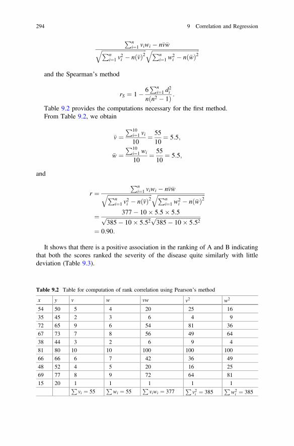
Pni¼1 viwi � n�v�wffiffiffiffiffiffiffiffiffiffiffiffiffiffiffiffiffiffiffiffiffiffiffiffiffiffiffiffiffiffiffiffiPn
i¼1 v2i � nð�vÞ2
q ffiffiffiffiffiffiffiffiffiffiffiffiffiffiffiffiffiffiffiffiffiffiffiffiffiffiffiffiffiffiffiffiffiffiPni¼1 w
2i � nð�wÞ2
qand the Spearman’s method
rS ¼ 1� 6Pn
i¼1 d2i
nðn2 � 1Þ :Table 9.2 provides the computations necessary for the first method.From Table 9.2, we obtain
�v ¼P10
i¼1 vi10
¼ 5510
¼ 5:5;
�w ¼P10
i¼1 wi
10¼ 55
10¼ 5:5;
and
r ¼Pn
i¼1 viwi � n�v�wffiffiffiffiffiffiffiffiffiffiffiffiffiffiffiffiffiffiffiffiffiffiffiffiffiffiffiffiffiffiffiffiPni¼1 v
2i � nð�vÞ2
q ffiffiffiffiffiffiffiffiffiffiffiffiffiffiffiffiffiffiffiffiffiffiffiffiffiffiffiffiffiffiffiffiffiffiPni¼1 w
2i � nð�wÞ2
q¼ 377� 10� 5:5� 5:5ffiffiffiffiffiffiffiffiffiffiffiffiffiffiffiffiffiffiffiffiffiffiffiffiffiffiffiffiffiffiffiffi
385� 10� 5:52p ffiffiffiffiffiffiffiffiffiffiffiffiffiffiffiffiffiffiffiffiffiffiffiffiffiffiffiffiffiffiffiffi
385� 10� 5:52p
¼ 0:90:
It shows that there is a positive association in the ranking of A and B indicatingthat both the scores ranked the severity of the disease quite similarly with littledeviation (Table 9.3).
Table 9.2 Table for computation of rank correlation using Pearson’s method
x y v w vw v2 w2
54 50 5 4 20 25 16
35 45 2 3 6 4 9
72 65 9 6 54 81 36
67 73 7 8 56 49 64
38 44 3 2 6 9 4
81 80 10 10 100 100 100
66 66 6 7 42 36 49
48 52 4 5 20 16 25
69 77 8 9 72 64 81
15 20 1 1 1 1 1Pvi ¼ 55
Pwi ¼ 55
Pviwi ¼ 377
Pv2i ¼ 385
Pw2i ¼ 385
294 9 Correlation and Regression
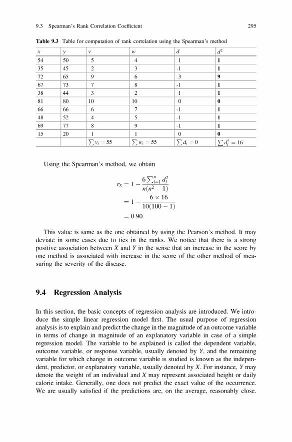
Using the Spearman’s method, we obtain
rS ¼ 1� 6Pn
i¼1 d2i
nðn2 � 1Þ¼ 1� 6� 16
10ð100� 1Þ¼ 0:90:
This value is same as the one obtained by using the Pearson’s method. It maydeviate in some cases due to ties in the ranks. We notice that there is a strongpositive association between X and Y in the sense that an increase in the score byone method is associated with increase in the score of the other method of mea-suring the severity of the disease.
9.4 Regression Analysis
In this section, the basic concepts of regression analysis are introduced. We intro-duce the simple linear regression model first. The usual purpose of regressionanalysis is to explain and predict the change in the magnitude of an outcome variablein terms of change in magnitude of an explanatory variable in case of a simpleregression model. The variable to be explained is called the dependent variable,outcome variable, or response variable, usually denoted by Y, and the remainingvariable for which change in outcome variable is studied is known as the indepen-dent, predictor, or explanatory variable, usually denoted by X. For instance, Y maydenote the weight of an individual and X may represent associated height or dailycalorie intake. Generally, one does not predict the exact value of the occurrence.We are usually satisfied if the predictions are, on the average, reasonably close.
Table 9.3 Table for computation of rank correlation using the Spearman’s method
x y v w d d2
54 50 5 4 1 135 45 2 3 -1 1
72 65 9 6 3 967 73 7 8 -1 138 44 3 2 1 181 80 10 10 0 066 66 6 7 -1 148 52 4 5 -1 169 77 8 9 -1 115 20 1 1 0 0P
vi ¼ 55P
wi ¼ 55P
di ¼ 0P
d2i ¼ 16
9.3 Spearman’s Rank Correlation Coefficient 295

The statistician usually wants to find the equation of the curve of best fit to expressthe relationship of the variables.
The regression analysis deals with studying the form of the relationship betweenthe variables in order to find a mathematical equation relating the outcome variableswith explanatory variables. Once the mathematical form of the relationship isdetermined, we can utilize it to predict the value of the response (dependent)variable (Y) by knowing the value of the predictor (independent) variable (X). Inother words, the objective of regression analysis is to estimate the mean of responsevariable (Y) by using the value of the predictor variable (X). For instance, we mightbe interested in predicting the blood pressure level of a person by using his weight,or predicting the height of an adult male by using the height of his father.
9.4.1 Simple Linear Regression Model
The first step in regression analysis is to estimate the model or the form of therelationship relating the response variable (Y) with the predictor or explanatoryvariable (X). One of the most useful relationships which has a lot of applications isthe linear relationship between response and predictor variables. The followingfigure presents some examples for linear and nonlinear relationships.
(a) linear relationship (b) linear relationship
(c) non-linear relationship (d) non-linear relationship
296 9 Correlation and Regression

If the relationship between Y and X is linear, then it can be represented by a linecalled the regression line. In this case, it is possible to fit a line on the scatterdiagram that describes this relationship. To introduce the simple linear regressionmodel, suppose that the random sample of paired variables are
ðX1; Y1Þ; ðX2; Y2Þ; . . .; ðXn; YnÞ:
We may state that the expectation of Y given X, EðY XÞj , is a linear regressionmodel or a regression function of Y upon X if it can be expressed as
EðY XÞj ¼ b0 þ b1X:
This model is called a simple regression model because it takes into account asingle independent variable X to explain the dependent variable, Y. There are tworegression parameters in this model which are unknown constants, b0 is an interceptand b1 is a slope known as the regression coefficient of the independent variable, X.Let us consider the relationship between the independent and dependent variablesfor a random sample, ðXi; YiÞ; i ¼ 1; . . .; n. The linear regression model for each pairof independent and dependent variables for the ith subject can be shown in thefollowing form
EðYi XiÞj ¼ b0 þ b1Xi; i ¼ 1; . . .; n:
Now, we can rewrite the model for each value of the outcome variable for acorresponding given value of Xi as follows
Yi ¼ b0 þ b1Xi þ ei; i ¼ 1; . . .; n
where the ei are the experimental errors and are distributed such that EðeiÞ ¼ 0 andVarðeiÞ ¼ r2, i = 1, …, n.
The above model includes an additional term because this is not a model for thepopulation mean based on given value of the independent variable, rather thismodel may contain error due to its deviation from the population mean which isshown in the following expression of the model
Yi ¼ E Yi Xijð Þþ ei;
where EðYi XiÞj ¼ b0 þ b1Xi; i ¼ 1; . . .; n: A comparison between the model for thepopulation mean for given values of independent variable and the relationshipbetween independent and dependent variables needs to be understood clearly inorder to interpret the results without any ambiguity.
The following assumptions are necessary for estimating the parameters of theregression model:
9.4 Regression Analysis 297

(i) The expected value of the error variable is zero, i.e., EðeiÞ ¼ 0 for all i;(ii) The variance of the error variable is VarðeiÞ ¼ r2 for all i;(iii) The error variables are independent, i.e., ei and ej are independent for any
i and j (i 6¼ j), and(iv) The independent variables and the error variables are independent, i.e.,
Xj and ei are independent for all i and j.
Under these assumptions, it can be shown that the least squares estimators ofb0 and b1 are minimum variance unbiased estimators (Best Linear UnbiasedEstimators). The least squares estimation procedure will be introduced in the nextsection.
A fifth assumption, the assumption that the residuals ej are normally distributed,though not needed for the least squares estimation but is needed to make confidenceinterval statements and to apply tests of significance:
(v) Normality: In conjunction with assumptions (i)–(iv), this assumption impliesthat ei �Nð0; r2Þ.
9.4.2 Estimation of b0 and b1
The parameters of the regression model, b0 and b1, are unknown population values.We have to estimate these parameters using the sample data. We have discussedabout estimation procedures in Chap. 7 and two methods of estimating parametersare highlighted there, one is the method of moments and the other one is the methodof maximum likelihood. For estimating the parameters of a regression model, wegenerally use a third method known as the method of least squares. The method ofleast squares is preferred for estimating parameters of a linear regression modelbecause of its good properties for the linear regression models, some of which willbe highlighted in this chapter. The most important criterion for employing the leastsquares method for estimating the parameters of a linear regression model is the factthat the error in fitting a linear regression model to the sample data is kept minimumthat provides the model fit a desirable acceptance to the users who prefer appli-cations to data with strong measurable properties.
The error term in the regression model is the deviation between the observedvalue of the dependent variable and the expected value of the dependent variable forgiven value of the independent variable which is
e ¼ Y � b0 þ b1Xð Þ:
Here, e represents the distance between the observed values of Y to the linerepresented by EðY XÞj ¼ b0 þ b1X which shows the error in representing theobserved values of Y by the regression line. We want to minimize
Pni¼1 e
2i such that
the estimates of the parameters confirm the minimum errors. For convenience, wedefine
298 9 Correlation and Regression

Q ¼Xni¼1
e2i ¼Xni¼1
Yi � b0 � b1Xið Þ2
where n denotes the number of observations in the sample. To minimize Q, we takethe partial derivative of Q with respect to each of the two parameters that we areestimating and set the resulting expressions equal to zero. Thus,
@Q@b0
¼ 2Xni¼1
Yi � b0 � b1Xið Þ �1ð Þ ¼ 0
and
@Q@b1
¼ 2Xni¼1
Yi � b0 � b1Xið Þ �Xið Þ ¼ 0
Dropping 2 and −1 from the estimating equations, the solutions for b0 and b1 areobtained by solving the equations which are generally called normal equations
Xni¼1
Yi � b0 � b1Xið Þ ¼ 0
Xni¼1
XiYi � b0Xi � b1X2i
� � ¼ 0
Solving the first normal equation and replacing b0 by b0 and b1 by b1, we obtain
nb0 ¼Xni¼1
Yi � b1Xni¼1
Xi
and the estimator of b0
b0 ¼ Y � b1X:
Similarly, the equation for b1 can be solved by expressing the equation in thefollowing form and replacing b0 by b0 and b1 by b1, we obtain
b1Xni¼1
X2i ¼ �b0
Xni¼1
Xi þXni¼1
XiYi
9.4 Regression Analysis 299
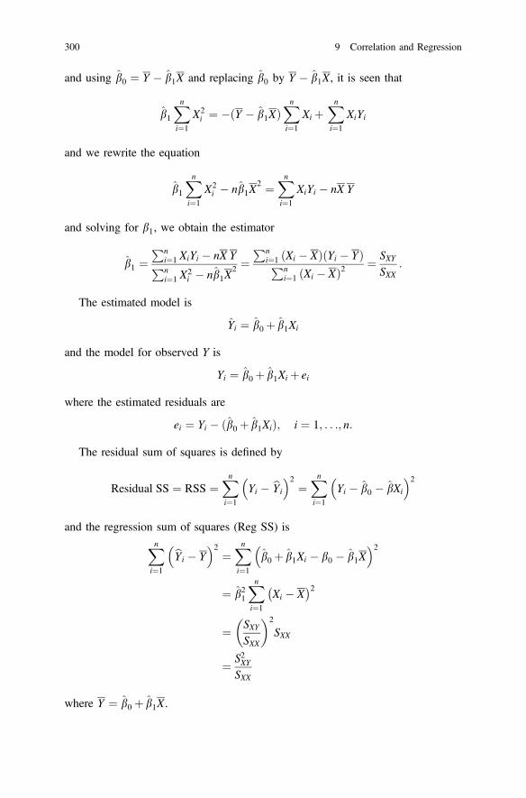
and using b0 ¼ Y � b1X and replacing b0 by Y � b1X, it is seen that
b1Xni¼1
X2i ¼ �ðY � b1XÞ
Xni¼1
Xi þXni¼1
XiYi
and we rewrite the equation
b1Xni¼1
X2i � nb1X
2 ¼Xni¼1
XiYi � nX Y
and solving for b1, we obtain the estimator
b1 ¼Pn
i¼1 XiYi � nX YPni¼1 X
2i � nb1X
2 ¼Pn
i¼1 ðXi � XÞðYi � YÞPni¼1 ðXi � XÞ2 ¼ SXY
SXX:
The estimated model is
Yi ¼ b0 þ b1Xi
and the model for observed Y is
Yi ¼ b0 þ b1Xi þ ei
where the estimated residuals are
ei ¼ Yi � ðb0 þ b1XiÞ; i ¼ 1; . . .; n:
The residual sum of squares is defined by
Residual SS ¼ RSS ¼Xni¼1
Yi � bYi
� 2¼Xni¼1
Yi � b0 � bXi
� 2and the regression sum of squares (Reg SS) isXn
i¼1
bYi � Y� 2
¼Xni¼1
b0 þ b1Xi � b0 � b1X� 2
¼ b21Xni¼1
Xi � X� �2
¼ SXYSXX
� �2
SXX
¼ S2XYSXX
where Y ¼ b0 þ b1X.
300 9 Correlation and Regression

The total sum of squares is
Total SS ¼Xni¼1
Yi � Y� �2
which can be rewritten and expanded in the following form
Xni¼1
Yi � Y� �2 ¼Xn
i¼1
Yi � bYi þ bYi � Y� 2
¼Xni¼1
Yi � bYi
� 2þXni¼1
bYi � Y� 2
þ 2Xni¼1
Yi � Yi� � bYi � Y
� :
In the product term, Yi � Yi ¼ ei and bYi � Y ¼ b1ðXi � XÞ. It can be shown thatthe product term is zero. Hence, the total sum of squares of the dependent variable,Y, can be partitioned into two components
Total SS ¼ SYY ¼Xni¼1
Yi � Y� �2¼Xn
i¼1
Yi � bYi
� 2þXni¼1
bYi � Y� 2
;
which can be rewritten as
SYY ¼ RSSþ S2XYSXX
and the residual sum of squares can be obtained from
RSS ¼ SYY � S2XYSXX
¼ SYY 1� S2XYSXXSYY
� �¼ SYY 1� r2XY
� �where the measure of Pearson’s correlation coefficient from the sample data isrXY ¼ SXY
SXXSYYthat shows the strength of linear relationship between variables X and Y.
It has been shown here that
Total SS ¼ Residual SSþRegression SS
which provides the important logical background for testing of hypothesesincluding the measure of goodness of fit of a regression model.
9.4 Regression Analysis 301

9.4.3 Interpretations of the Parameters of the RegressionLine
The parameters of the population regression model, Y ¼ bo þ b1Xþ e, are b0 andb1. The first parameter, b0, is the intercept of the line; it is the value of Y whenX = 0. The second parameter, b1, is the slope of the regression line; it is the amountof change in the value of Y, on average, when the value of X is increased by oneunit. In particular, the value of b1 determines the nature of the linear relationshipbetween X and Y. If there is no linear relationship between X and Y, then b1 ¼ 0; ifthere is a positive linear relationship, then b1 [ 0; if there is a negative linearrelationship, then b1\0. The estimated regression model is bY ¼ b0 þ b1X and theobserved value of the dependent variable can be shown as Y ¼ b0 þ b1Xþ e ¼Y þ e, where e is the estimated error from the sample data.
The estimates of b0 and b1 that minimize the differences between the observedvalues of the dependent variable and the regression line are called the least squaresestimates. The vertical differences between the scatter points and the regression lineare illustrated in the following figure
9.4.4 Properties of the Least Squares Estimatorsand the Fitted Regression Model
The least squares estimators b0 and b1 have several important properties. Some ofthe properties are discussed here. Let us consider the least squares estimators
b0 ¼ Y � b1X;
and
b1 ¼Pn
i¼1 Xi � X� �
Yi � Y� �Pn
i¼1 Xi � X� �2 :
The above estimators are linear combinations of the observations, Yi. Forexample
302 9 Correlation and Regression

b1 ¼Pn
i¼1 Xi � X� �
Yi � Y� �Pn
i¼1 Xi � X� �2
¼Pn
i¼1 Xi � X� �
YiPni¼1 Xi � X� �2
¼Xni¼1
CiYi
whereXi�Xð ÞPn
i¼1Xi�Xð Þ2 ¼ Ci and
Pni¼1 Xi � X� �
X ¼ 0:
(i) The least squares estimators b0 and b1 are unbiased estimators of modelparameters b0 and b1. To show this for b1, let us consider
E b1�
¼ EXni¼1
CiYi
!
¼Xni¼1
CiEðYiÞ
¼Xni¼1
Ciðb0 þ b1XiÞ
¼ b0Xni¼1
Ci þ b1Xni¼1
CiXi:
It can be shown from the linear function thatPn
i¼1 Ci ¼ 0 andPn
i¼1 CiXi ¼ 1,and using these results we prove the following property of the least squaresestimator
E b1�
¼ b0 � 0þ b1 � 1 ¼ b1
which proves that b1 is an unbiased estimator of b1.
(ii) The estimator b0 is an unbiased estimator of b0 .
We know that b0 ¼ Y � b1X .The expected value of b0 is
Eðb0Þ ¼ EðYÞ � XEðb1Þ¼ b0 þ b1X � b1X
¼ b0
confirming that b0 is an unbiased estimator of b0.
9.4 Regression Analysis 303
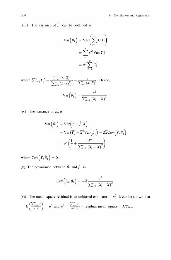
(iii) The variance of b1 can be obtained as
Var b1�
¼ VarXni¼1
CiYi
!
¼Xni¼1
C2i VarðYiÞ
¼ r2Xni¼1
C2i
wherePn
i¼1 C2i ¼
Pn
i¼1Xi�Xð Þ2Pn
i¼1Xi�Xð Þ2
� �2 ¼ 1Pn
i¼1Xi�Xð Þ2 : Hence,
Var b1�
¼ r2Pni¼1 Xi � X� �2 :
(iv) The variance of b0 is
Var b0�
¼ Var Y � b1X�
¼ Var Y� �þX
2Var b1�
� 2XCov Y ; b1�
¼ r21nþ X
2Pni¼1 Xi � X� �2
!
where Cov Y ; b1�
¼ 0.
(v) The covariance between b0 and b1 is
Cov b0; b1�
¼ �Xr2Pn
i¼1 Xi � X� �2 :
(vi) The mean square residual is an unbiased estimator of r2. It can be shown that
EPn
i¼1e2i
ðn�2Þ
� �¼ r2 and r2 ¼
Pn
i¼1e2i
ðn�2Þ = residual mean square = MSRes.
304 9 Correlation and Regression

From the above equation, it can be shown that the expected value of the errormean square is the variance
E
Pni¼1 e
2i
n� 2
� �¼ r2
which implies that the error mean square is an unbiased estimator of the variance.
Example 9.4The data set we have used for computing the Pearson’s correlation coefficient isemployed, here, for showing the estimation and tests for the simple regressionmodel introduced in this section. We have considered weight (kg) and height(cm) of 12 children under 5 years of age drawn randomly. The estimation and testsfor simple regression model for variables height (X) and weight (Y) of childrenunder 5 years of age are shown here.
Table 9.4 shows the computations necessary for estimating parameters of theregression model
Yi ¼ b0 þ b1Xi þ ei; i ¼ 1; . . .; 12:
The least squares estimators of b0 and b1 are
b0 ¼ Y � b1X;
Table 9.4 Height (x) and weight (y) of 12 children under 5 years of age and calculationsnecessary for estimating the parameters of a simple regression model
xHeight (cm)
yWeight (kg)
xy x2 y2
72.1 7.4 533.54 5198.41 54.76
93.5 11.3 1056.55 8742.25 127.69
78.9 9.8 773.22 6225.21 96.04
85.2 12.1 1030.92 7259.04 146.41
89.1 11.6 1033.56 7938.81 134.56
100.3 13.2 1323.96 10060.09 174.24
92.5 11.5 1063.75 8556.25 132.25
93.5 12.2 1140.70 8742.25 148.84
97.7 12.3 1201.71 9545.29 151.29
79.9 10.5 838.95 6384.01 110.25
83.2 9.3 773.76 6922.24 86.49
68.8 6.6 454.08 4733.44 43.56Px ¼ 1034:7
Py ¼ 127:8
Pxy ¼ 11224:7
Px2 ¼ 90307:29
Py2 ¼ 1406:38
9.4 Regression Analysis 305
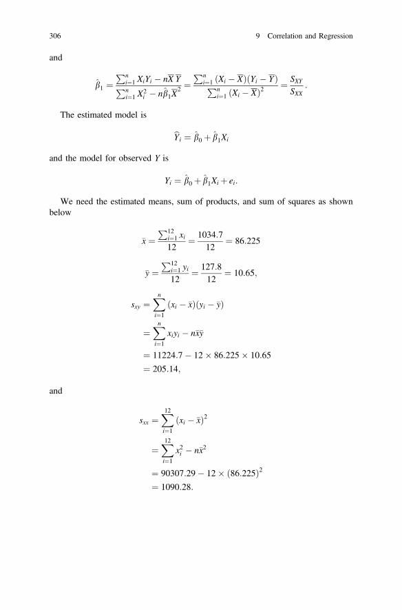
and
b1 ¼Pn
i¼1 XiYi � nX YPni¼1 X
2i � nb1X
2 ¼Pn
i¼1 ðXi � XÞðYi � YÞPni¼1 ðXi � XÞ2 ¼ SXY
SXX:
The estimated model is
bYi ¼ b0 þ b1Xi
and the model for observed Y is
Yi ¼ b0 þ b1Xi þ ei:
We need the estimated means, sum of products, and sum of squares as shownbelow
�x ¼P12
i¼1 xi12
¼ 1034:712
¼ 86:225
�y ¼P12
i¼1 yi12
¼ 127:812
¼ 10:65;
sxy ¼Xni¼1
ðxi � �xÞðyi � �yÞ
¼Xni¼1
xiyi � n�x�y
¼ 11224:7� 12� 86:225� 10:65
¼ 205:14;
and
sxx ¼X12i¼1
ðxi � �xÞ2
¼X12i¼1
x2i � n�x2
¼ 90307:29� 12� ð86:225Þ2¼ 1090:28:
306 9 Correlation and Regression

The estimates of regression parameters are
b1 ¼Pn
i¼1 xiyi � n�x�yPni¼1 x
2i � n�x2
¼ 205:141090:28
¼ 0:1882
b0 ¼ �y� b1�x
¼ 10:65� 0:1882� 86:225
¼ �5:5775:
The fitted model is
bYi ¼ b0 þ b1Xi
¼ �5:5775þ 0:1882Xi
and the model for observed Y is
Yi ¼ b0 þ b1Xi þ ei¼ �5:5775þ 0:1882Xi þ ei:
The estimated error can be obtained as
ei ¼ Yi � ð�5:5775þ 0:1882XiÞ:
We know that the unbiased estimator of the population variance r2 is the meansquare error s2 from the sample data. The mean square error computed from thesample data is shown in below (Table 9.5)
s2 ¼Pni¼1
ðyi � yiÞ2
n� 2¼ 6:7104
10¼ 0:67104:
9.4.5 Hypothesis Testing on the Slope and Intercept
We are often interested in testing hypotheses and constructing confidence intervalsabout the model parameters. These procedures require that we make the additionalassumption that the model errors ei are normally distributed. Thus, we add tocomplete the assumptions by stating that the errors are normally and independentlydistributed with mean 0 and variance r2, abbreviated NIDð0; r2Þ.
9.4 Regression Analysis 307

Tests for the Parameters
Suppose that we wish to test the hypothesis that the slope equals a constant, say b10.The appropriate hypotheses are
H0: b1 ¼ b10
H1: b1 6¼ b10where a two-sided alternative is specified. Since the errors ei are NIDð0; r2Þ, the
observations Yi are NIDðb0 þ b1Xi; r2Þ. Now b1 is a linear combination of theobservations, so b1 is normally distributed with mean b1 and variance r2=SXX usingthe mean and variance of b1 as shown earlier. Therefore, the statistic
Z ¼ b1 � b10ffiffiffiffiffiffiffiffiffiffiffiffiffiffir2=SXX
pis distributed Nð0; 1Þ if the null hypothesis is true. If r2 were known, we could useZ to test the null hypothesis. Generally, r2 is unknown. We have already seen thatMSRes is an unbiased estimator of r2. It can be shown that ðn� 2ÞMSRes=r2 followsa v2n�2 distribution and that MSRes and b1 are independent. By the definition of at statistic,
Table 9.5 Height (x) and weight (y) of 12 children under 5 years of age and calculationsnecessary for estimating the variance
xHeight (cm)
yWeight (kg)
y ei e2i
72.1 7.4 7.99172 −0.59172 0.350133
93.5 11.3 12.0192 −0.7192 0.517249
78.9 9.8 9.27148 0.52852 0.279333
85.2 12.1 10.45714 1.64286 2.698989
89.1 11.6 11.19112 0.40888 0.167183
100.3 13.2 13.29896 -0.09896 0.009793
92.5 11.5 11.831 −0.331 0.109561
93.5 12.2 12.0192 0.1808 0.032689
97.7 12.3 12.80964 −0.50964 0.259733
79.9 10.5 9.45968 1.04032 1.082266
83.2 9.3 10.08074 −0.78074 0.609555
68.8 6.6 7.37066 −0.77066 0.593917Px ¼ 1034:7
Py ¼ 127:8 127.8005 6.7104
308 9 Correlation and Regression

T ¼ b1 � b10ffiffiffiffiffiffiffiffiffiffiffiffiffiffiffiffiffiffiffiffiffiMSRes=SXX
pfollows a tn�2 distribution if the null hypothesis is true. The degree of freedomassociated with t is the degree of freedom associated with MSRes. The nullhypothesis is rejected if
tj j[ tðn�2Þ;1�a=2:
The denominator of this test statistic, t, is often called the estimated standarderror or simply, the standard error of the slope. That is,
seðb1Þ ¼ffiffiffiffiffiffiffiffiffiffiffiffiMSResSXX
r:
Therefore, we often see T written as
T ¼ b1 � b10seðb1Þ
:
A similar procedure can be used to test hypothesis about the intercept. To test
H0: b0 ¼ b00
H1: b0 6¼ b00
we would use the following test statistic:
T ¼ b0 � b00ffiffiffiffiffiffiffiffiffiffiffiffiffiffiffiffiffiffiffiffiffiffiffiffiffiffiffiffiffiffiffiMSRes 1
n þ X2
SXX
� r ¼ b0 � b00seðb0Þ
where seðb0Þ ¼ffiffiffiffiffiffiffiffiffiffiffiffiffiffiffiffiffiffiffiffiffiffiffiffiffiffiffiffiffiffiffiffiffiffiffiffiffiffiffiffiffiffiffiMSResð1=nþX
2=SXXÞ
qis the standard error of the intercept. We
may reject the null hypothesis if
tj j[ tðn�2Þ;1�a=2:
9.4 Regression Analysis 309

9.4.6 Testing Significance of Regression
A very important special case of the hypothesis is
H0: b1 ¼ 0
H1: b1 6¼ 0
These hypotheses relate to the significance of regression. Failing to rejectH0: b1 ¼ 0 implies that there is no linear relationship between X and Y. This mayimply either of the following:
(i) X is of little value in explaining the variation in Y and that the best estimator ofY for any X is bY ¼ Y ;
(ii) The true relationship between X and Y is not linear. Therefore, failing to rejectH0: b1 ¼ 0 is equivalent to saying that there is no linear relationship betweenX and Y.
Alternatively if H0: b1 ¼ 0 is rejected, this implies that X is of value inexplaining the variability in Y. However, rejecting H0: b1 ¼ 0 could mean either ofthe following:
(i) that the straight-line model is adequate;(ii) better results could be obtained with the addition of higher order polynomial
terms in X.
The test procedure for H0: b1 ¼ 0 is as follows:
T ¼ b1seðb1Þ
:
The hypothesis of significance of regression would be neglected if
tj j[ tðn�2Þ;1�a=2:
9.4.7 Analysis of Variance
We may also use an analysis of variance approach to test the significance of aregression. The analysis of variance is based on a partitioning of total variability inthe response variable Y. To obtain this partitioning, let us begin with
Yi � Y ¼ ðbYi � YÞþ ðYi � bYiÞ:
310 9 Correlation and Regression

Squaring both sides of the above equation and summing over all n observationsproduces
Xni¼1
ðYi � YÞ2 ¼Xni¼1
ðbYi � YÞ2 þXni¼1
ðYi � bYiÞ2 þ 2Xni¼1
ðbYi � YÞðYi � bYiÞ:
The product term can be rewritten as
2Xni¼1
ðbYi � YÞðYi � bYiÞ ¼ 2Xni¼1
bYiðYi � bYiÞ � 2YXni¼1
ðYi � bYiÞ
¼ 2Xni¼1
bYiei � 2YXni¼1
ei ¼ 0
wherePn
i¼1 ei ¼ 0 andPn
i¼1bYiei ¼ 0.
Therefore,
Xni¼1
ðYi � YÞ2 ¼Xni¼1
ðbYi � YÞ2 þXni¼1
ðYi � bYiÞ2:
This equation is the fundamental analysis of variance identity for a regressionmodel. Symbolically, we usually write
SSTotal ¼ SSReg þ SSRes:
The total sum of squares, SSTotal, has dfT ¼ n� 1 degrees of freedom due toreduction of one degree of freedom resulting from the constraint
Pni¼1 ðYi � YÞ on
the deviations Yi � Y . There are two components in the analysis of variance,regression, and residual. It has been shown that SSReg is completely determined by
one parameter, namely, b1, and SSReg ¼ b1SXY , hence dfReg ¼ 1 degree of freedom.
The component of residual sum of squares is obtained from the deviations Yi � bYi,where bYi depends on estimates b0 and b1 . The number of parameters estimated forcomputing SSRes causes reduction in the degrees of freedom and dfRes ¼ n� 2.Hence, it is shown that
dfTotal ¼ dfReg þ dfResðn� 1Þ ¼ 1þðn� 2Þ:
We can use the usual analysis of variance F test to test the hypothesisH0: b1 ¼ 0. By definition
9.4 Regression Analysis 311

F ¼ SSReg=dfRegSSRes=dfRes
¼ SSReg=1SSRes=ðn� 2Þ ¼
MSRegMSRes
follows the F1;ðn�2Þ distribution. Therefore, to test the hypothesis H0: b1 ¼ 0, teststatistic is computed and the null hypothesis is rejected if
F[Fa;1;ðn�2Þ:
The test procedure is summarized in Table 9.6The t statistic as defined earlier is
T ¼ b1seðb1Þ
¼ b1ffiffiffiffiffiffiffiffiffiffiffiffiffiffiffiffiffiffiffiffiffiffiMSRes=SSX
pcould be used for testing for significance of regression. However, squaring bothsides, we obtain
T2 ¼ b21SSXMSRes
¼ b1SXYMSRes
¼ MSRegMSRes
:
Thus, T2 is identical to F of the analysis of variance approach for the special casewhere the square of a T variable with (n − 2) degrees of freedom is equivalent to anF variable with 1 and (n − 2) degrees of freedom. For testing the null hypothesisH0: b1 ¼ 0 in a simple regression problem, the t-test has advantages becauseone-sided alternatives such as H1: b1\0 or H1: b1 [ 0 can also be performedusing the t-test.
9.4.8 Interval Estimation in Simple Linear Regression
Under the assumption that ei �NIDð0; r2Þ, it can be shown that
(i) b0 has a normal distribution with mean b0 and variance
Table 9.6 The analysis of variance table for a simple regression model
Source ofvariation
Sum of square df Mean squares F
Regression SSReg ¼ b1SXY � nY2 1 SSReg=1 F ¼ MSReg=MSRes
Residual SSRes ¼ SSTotal � b1SXy n − 2 SSRes=ðn� 2Þ
312 9 Correlation and Regression

Varðb0Þ ¼ r21nþ X
2
SXX
!:
(ii) b1 has a normal distribution with mean b1 and variance Varðb1Þ ¼ r2=SXX .(iii) Covðb0; b1Þ ¼ r2ð�X=SXXÞ.(iv) Residual SS, RSS ¼ SYY � ðS2XY=SXXÞ; then RSS=r2 has a v2 distribution with
ðn� 2Þ df and r2 ¼ RSS=ðn� 2Þ is an unbiased estimator for r2.(v) If we substitute r2 for r2 in Vðb0Þ and Vðb1Þ given in (i) and (ii), we obtain
the estimated variances
Varðb0Þ ¼ r21nþ X
2
SXX
!;
and
Varðb1Þ ¼r2
SXX
where r2 ¼Pn
i¼1e2i
ðn�2Þ is the mean square residual denoted by s2 ¼Pn
i¼1Yi�bYi
� �2ðn�2Þ ,
which is an unbiased estimator of r2.Test statistics for the regression parameters are
T ¼ b0 � b0seðb0Þ
� tn�2
T ¼ b1 � b1seðb1Þ
� tn�2:
Therefore, a 100ð1� aÞ% confidence interval on the slope b1 is given by
b1 � tðn�2Þ;1�a=2seðb1Þ� b1 � b1 þ tðn�2Þ;1�a=2seðb1Þ:
Similarly, a 100ð1� aÞ% confidence interval on the intercept b0 is given by
b0 � tðn�2Þ;1�a=2seðb0Þ� b0 � b0 þ tðn�2Þ;1�a=2seðb0Þ:
The interpretation of confidence interval for parameters b1 and b0: If we repeattaking samples of size n from the same population very large number of times and ifwe construct confidence interval for each parameter from each sample then the
9.4 Regression Analysis 313

proportion of those intervals that will include the true population value (b1 in thefirst confidence interval and b0 in the second interval) is 1� a.
If the errors are normally and independently distributed then the sampling dis-tribution of
ðn� 2ÞMSResr2
� v2n�2:
Thus,
P½v2ðn�2Þ;a=2 � ðn�2ÞMSResr2 � v2ðn�2Þ;1�a=2� ¼ 1� a: and consequently a 100ð1�
aÞ% confidence interval on r2 is
Pðn� 2ÞMSResv2ðn�2Þ;1�a=2
� r2 � ðn� 2ÞMSResv2ðn�2Þ;a=2
" #¼ 1� a:
9.4.9 Interval Estimation of Mean Response
In many situations of applications of regression models, the estimation of meanresponse is of major concern. This problem involves estimation of the meanresponse, EðYÞ, for a given value of the independent variable, X. For example, letX0 be the given value of X for which we wish to estimate the mean response, sayEðY jX0Þ. Let us assume that X0 is any value within the range of the sample data onthe independent variable, X. The expected value, EðY jX0Þ, is
bEðY X0j Þ ¼ b0 þ b1X0:
To obtain a 100ð1� aÞ% confidence interval of EðY jX0Þ, we need to find thesampling distribution of bEðY jX0Þ. It can be shown that
EðY X0j Þ ¼ b0 þ b1X0
and the variance of bEðY jX0Þ is
Var½bEðY jX0Þ� ¼ Var½Y þ b1ðX0 � XÞ�
¼ r2
nþ r2ðX0 � XÞ2
SSX
¼ r21nþ ðX0 � XÞ2
SSX
" #:
314 9 Correlation and Regression

Then, it follows that
bEðY X0j Þ ¼ b0 þ b1X0 �N b0 þ b1X0; r2 1nþ ðX0 � XÞ2
SSX
" # !:
It can be shown that covðY ; b1Þ ¼ 0. Thus, the sampling distribution of
T ¼bEðY=X0Þ � EðY=X0ÞffiffiffiffiffiffiffiffiffiffiffiffiffiffiffiffiffiffiffiffiffiffiffiffiffiffiffiffiffiffiffiffiffiffiffiffiffiffiffiMSRes 1
n þ ðX0�XÞ2SSX
� ris t with n − 2 degrees of freedom. Consequently, a 100ð1� aÞ% confidenceinterval on the mean response at the point X ¼ X0 is
bEðY=X0Þ � tðn�2Þ;1�a=2
ffiffiffiffiffiffiffiffiffiffiffiffiffiffiffiffiffiffiffiffiffiffiffiffiffiffiffiffiffiffiffiffiffiffiffiffiffiffiffiffiffiffiffiffiffiffiffiffiMSRes
1nþ ðX0 � XÞ2
SSX
!vuut �EðY=X0Þ
� bEðY=X0Þþ tðn�2Þ;1�a=2
ffiffiffiffiffiffiffiffiffiffiffiffiffiffiffiffiffiffiffiffiffiffiffiffiffiffiffiffiffiffiffiffiffiffiffiffiffiffiffiffiffiffiffiffiffiffiffiffiMSRes
1nþ ðX0 � XÞ2
SSX
!vuut :
Interval Estimation of Prediction
Let the regression equation be
bY ¼ b0 þ b1X
is used for predicting Y for given values of X.Let XF be a future value of X. Then, we predict the corresponding value of Y by
bYF ¼ b0 þ b1XF :
The true value of YF is
YF ¼ b0 þ b1XF þ eF :
Hence, the prediction error is
bYF � YF ¼ ðb0 � b0Þþ ðb1 � b1ÞXF � eF
9.4 Regression Analysis 315

and
EðbYF � YFÞ ¼ Eðb0 � b0ÞþEðb1 � b1ÞXF � EðeFÞ ¼ 0:
Then, the variance is
VarðbYF � YFÞ ¼ Varðb0 � b0ÞþX2FVarðb1 � b1Þ
þ 2XFCovðb0 � b0; b1 � b1ÞþVarðeFÞ
¼ r21nþ X
2
SXX
!þ r2:
X2F
SXX� 2XFr
2:XSXX
þ r2
¼ r2 1þ 1nþ ðXF � XÞ2
SXX
" #:
The estimated variance is
VarðbYF � YFÞ ¼ MSRes 1þ 1nþ ðXF � XÞ2
SXX
" #:
Consequently, a 100ð1� aÞ% prediction interval on a future observation at thepoint X ¼ XF is
bYF � tðn�2Þ;1�a=2
ffiffiffiffiffiffiffiffiffiffiffiffiffiffiffiffiffiffiffiffiffiffiffiffiffiffiffiffiffiffiffiffiffiffiffiffiffiffiffiffiffiffiffiffiffiffiffiffiffiffiffiffiffiffiffiffiffiMSRes 1þ 1
nþ ðXF � XÞ2
SSX
!vuut � YF
� bYF þ tðn�2Þ;1�a=2
ffiffiffiffiffiffiffiffiffiffiffiffiffiffiffiffiffiffiffiffiffiffiffiffiffiffiffiffiffiffiffiffiffiffiffiffiffiffiffiffiffiffiffiffiffiffiffiffiffiffiffiffiffiffiffiffiffiMSRes 1þ 1
nþ ðXF � XÞ2
SSX
!vuutThe prediction interval widens with an increase in the distance between
XF and X and is minimum at X ¼ XF .
9.4.10 Coefficient of Determination of the Regression Model
The coefficient of determination is a quantitative measure used to evaluate theappropriateness and the adequacy of fitting the assumed regression model to thesample data in terms of the performance of the model in explaining the variation in Y.
The coefficient of determination is denoted by R2. It measures the proportion ofvariation in the values of Y that can be explained by the regression model. The totalvariation in the values of Y is measured by the quantity
Pni¼1 ðYi � YÞ2.
316 9 Correlation and Regression
The coefficient of determination is defined by
R2 ¼Pn
i¼1 ðYi � �YÞ2Pni¼1 ðYi � �YÞ2 ¼
SSRegSSTotal
where
bY i ¼ b0 þ b1Xi; i ¼ 1; 2; . . .; n:
Alternatively,
R2 ¼ 1�Pn
i¼1 ðYi � YiÞ2Pni¼1 ðYi � �YÞ2 ¼ 1� SSRes
SSTotal:
The coefficient of determination, R2, can be shown as the squared correlationbetween Y and bY and it measures the proportion of total variation about the mean Yexplained by the regression model. If we multiply the coefficient of multipledetermination by 100 then it interprets percentage of total variation about the meanexplained by the regression model. The coefficient of determination ranges between0 and 1, a value near zero indicates that the regression model either fails or performspoorly to explain the total variation and a value near 1 indicates that the regressionmodel explains the total variation either with near perfection or performs very well.A large value of R2 shows that the regression model performs strongly in explainingthe variation of the response variable by the explanatory variable included in themodel.
Some important characteristics of R2 are summarized below.
1. The value of R2 is between zero and one, both inclusive, i.e., 0�R2 � 1.2. The larger the value of R2 the better the regression model explains the variation
of Y.3. Large values of R2 indicate that the regression model fits the observation very
well. Small values of R2 indicate that the regression model does not fit theobservation well.
4. If R2 ¼ 1, then the regression model explains all variations of Y, which meansthat all observations lie on the regression line, i.e., there is a perfect correlationbetween Y and X.
5. If R2 ¼ 0, then the regression model cannot explain the variation of Y at all,which means there is no linear relationship between Y and X.
6. We can show that
R2 ¼ 1�Pn
i¼1 ðYi � bYiÞ2Pni¼1 ðYi � YÞ2
9.4 Regression Analysis 317
which implies that if the residual sum of squares decreases then R2 increases and ifthe residual sum of squares increases then R2 decreases. This provides the funda-mental measure of the fit of a regression model to the sample data.
Example 9.5For the data in the previous example, let us illustrate the interval estimation ofparameters and tests for the model and parameters. The following results aresummarized from the previous example:
�x ¼ 86:225; �y ¼ 10:65; sxy ¼ 205:14; sxx ¼ 1090:28:
We can also compute the total sum of squares of the dependent variable Y fromthe sample data as
syy ¼Xni¼1
ðyi � �yÞ2
¼Xni¼1
y2i � n�y2
¼ 45:309:
The estimates of regression parameters are b0 ¼ �5:5775 and b1 ¼ 0:1882. Thefitted model is
bYi ¼ �5:5775þ 0:1882Xi
and the model for observed Y is
Yi ¼ b0 þ b1Xi þ ei¼ �5:5775þ 0:1882Xi þ ei:
The estimated error can be obtained as
ei ¼ Yi � ð�5:5775þ 0:1882XiÞ:
Table 9.7 provides necessary calculations for estimating the variance.We know that the unbiased estimator of the population variance r2 is the mean
square error s2 from the sample data. The mean square error computed from thesample data is shown below
s2 ¼Pn
i¼1 ðyi � yiÞ2n� 2
¼ 6:710410
¼ 0:67104:
The error sum of squares is 6.7104.
318 9 Correlation and Regression

Subtracting the error sum of squares from the total sum of squares of Y, weobtain the regression sum of squares for the model which is
the regression sum of squares =Pn
i¼1 ðyi � yÞ2= syy − error sum of squares= 45.309 − 6.710 = 38.599.A 95% confidence interval for b1 using the sample data is obtained by
computing
b1 � tðn�2Þ;1�a=2
ffiffiffiffiffiffiffis2
sXX
s
which is
0:1882� t10;0:975
ffiffiffiffiffiffiffiffiffiffiffiffiffiffiffiffi0:671041090:28
r¼ 0:1882� 2:228� 0:0248
¼ 0:1882� 0:0553:
The 95% confidence interval for b1 is (0.1329, 0.2453) and notice that theinterval does not include the null value.
(ii) Calculating the coefficient of determination (R2)
(a) First method: using the formula R2 ¼Pni¼1 ðbYi � YÞ2=Pn
i¼1 ðYi � YÞ2:
Table 9.7 Height (X) and Weight (Y) of 12 children under 5 years of age and calculationsnecessary for estimating the variance
xHeight (cm)
yWeight (kg)
y ei e2i
72.1 7.4 7.99172 −0.59172 0.350133
93.5 11.3 12.0192 −0.7192 0.517249
78.9 9.8 9.27148 0.52852 0.279333
85.2 12.1 10.45714 1.64286 2.698989
89.1 11.6 11.19112 0.40888 0.167183
100.3 13.2 13.29896 −0.09896 0.009793
92.5 11.5 11.831 −0.331 0.109561
93.5 12.2 12.0192 0.1808 0.032689
97.7 12.3 12.80964 -0.50964 0.259733
79.9 10.5 9.45968 1.04032 1.082266
83.2 9.3 10.08074 −0.78074 0.609555
68.8 6.6 7.37066 −0.77066 0.593917Px ¼ 1034:7
Py ¼ 127:8
Pyi ¼ 127:08 6.7104
9.4 Regression Analysis 319

R2 ¼Pn
i¼1 ðbYi � YÞ2Pni¼1 ðYi � YÞ2 ¼ 38:599
45:309¼ 0:8519:
The positive square root of the coefficient of determination is
R ¼ 0:9229:
Since the value of coefficient of determination is R2 ¼ 0:8519, we conclude that85% of the total variation in the values of Y can be explained by the regressionmodel.
(b) Second method: using the formula R2 ¼ r2:
In a previous example, we have found that the Pearson’s coefficient of corre-lation is r ¼ þ 0:9229. Therefore, the coefficient of determination is
R2 ¼ r2 ¼ ðþ 0:9229Þ2 ¼ 0:8519:
9.4.11 Tests for the Parameters
The tests for the regression parameters are illustrated using the sample data. Thenull and alternative hypotheses for b1 are
H0: b1 ¼ 0
H1: b1 6¼ 0
where a two-sided alternative is specified. Here the error ei is NIDð0;r2Þ, therandom variables Yi is NIDðb0 þ b1Xi; r2Þ. The test statistic is
Z ¼ b1 � 0ffiffiffiffiffiffiffiffiffiffiffiffiffiffir2=SXX
pif r2 is known. However, as r2 is unknown and we know that MSRes ¼ s2 is anunbiased estimator of r2, the test statistic for unknown variance is
T ¼ b1 � b10ffiffiffiffiffiffiffiffiffiffiffiffiffiffiffiffiffiffiffiffiffiMSRes=SXX
pwhich follows a tn�2 distribution if the null hypothesis is true. The degree offreedom associated with t is the degree of freedom associated with MSRes. We mayreject the null hypothesis if
320 9 Correlation and Regression

tj j[ tðn�2Þ;1�a=2:
Therefore, the value of t statistic from the sample data is
t ¼ b1 � 0
seðb1Þ
¼ b1ffiffiffiffiffiffiffiffiffiffiffiffis2=sxx
p¼ 0:1882ffiffiffiffiffiffiffiffiffiffiffiffiffiffiffiffiffiffiffiffiffiffiffiffiffiffiffiffiffiffiffiffi
0:6710=1090:28p
¼ 7:5862
and the critical values are t10;0:025 ¼ �2:228 and t10;0:975 ¼ 2:228. The test statisticvalue falls in the critical region so the null hypothesis of no relationship betweenheight and weight of children under 5 years of age may be rejected.
Similarly, to test hypothesis about the intercept
H0: b0 ¼ 0
H1: b0 6¼ 0
we can use the test statistic
T ¼ b0 � 0ffiffiffiffiffiffiffiffiffiffiffiffiffiffiffiffiffiffiffiffiffiffiffiffiffiffiffiffiffiffiffiMSRes 1
n þ X2
SXX
� r ¼ b0seðb0Þ
where seðb0Þ ¼ffiffiffiffiffiffiffiffiffiffiffiffiffiffiffiffiffiffiffiffiffiffiffiffiffiffiffiffiffiffiffiffiffiffiffiffiffiffiffiffiffiffiffiMSResð1=nþX
2=SXXÞ
qis the standard error of the intercept. We
may reject the null hypothesis if
tj j[ tðn�2Þ;1�a=2:
We can compute the value of the test statistic using the sample data
t ¼ b0ffiffiffiffiffiffiffiffiffiffiffiffiffiffiffiffiffiffiffiffiffiffiffiffiffiffiffiffiffiffiMSRes 1
n þ �x2sxx
� r¼ �5:5775ffiffiffiffiffiffiffiffiffiffiffiffiffiffiffiffiffiffiffiffiffiffiffiffiffiffiffiffiffiffiffiffiffiffiffiffiffiffiffiffiffiffiffi
0:6710 112 þ ð86:225Þ2
1090:28
� r¼ �2:5917
9.4 Regression Analysis 321

and we have shown that the critical values are t10;0:025 ¼ �2:228 andt10;0:975 ¼ 2:228. This test also shows that the null hypothesis may be rejectedbecause the test statistic value from the sample data falls in the critical at 5% levelof significance.
9.4.12 Testing Significance of Regression
The test for model, in case of the simple regression is similar to testing the t-testperformed for the regression parameter, b1. The null and alternative hypotheses are
H0: b1 ¼ 0
H1: b1 6¼ 0:
These hypotheses relate to the significance of regression. Failing to rejectH0: b1 ¼ 0 implies that there is no linear relationship between X and Y.
The test procedure for H0: b1 ¼ 0 is shown for the sample data already. This is aspecial case for simple regression model only. To generalize the procedure formultiple regression model, we need to use the analysis of variance procedure whichis illustrated below.
Analysis of VarianceThe analysis of variance procedure is based on the components of variance from thefact that
Total SS = Regression SS + Error SS., which is expressed previously as
SSTotal ¼ SSReg þ SSRes:
The test procedure is summarized in Table 9.8.The test statistic for testing H0: b1 ¼ 0 is
F ¼ MSRegMSRes
¼ 38:5990:671
¼ 57:525
follows the F1;10 distribution. The critical region is defined by
F[F0:05;1;10
where F0:05;1;10 ¼ 4:96. The test statistic value from the sample data is 57.525 thatfalls in the critical region, hence, we may reject the null hypothesis that there is nolinear relationship between height and weight. It may be shown thatF0:05;1;10 ¼ t2
0:025;10¼ ð2:228Þ2 ¼ 4:96.
322 9 Correlation and Regression

9.5 Multiple Linear Regression
A regression model that involves more than one regressor variable is called amultiple regression model. The simple regression model is introduced in previoussections and we extend the simple regression for several independent variables inthis section, so that the regression model for an outcome variable can be expressedas a linear function of several explanatory variables. In many instances the outcomeor response variable cannot be explained adequately by a single independentvariable rather there may multiple factors that may cause change in the outcomevariable. A multiple regression model that might describe this relationship is
E Y X1;X2;X3jð Þ ¼ b0 þ b1X1 þ b2X2 þ b3X3
which can also be expressed in the following form for the random sample ofvariables Y ;X1;X2 and X3
Y ¼ b0 þ b1X1 þ b2X2 þ b3X3 þ e
where Y denotes the response variable, X1, X2 and X3 denote the explanatory orindependent variables 1, 2, and 3. This is the multiple linear regression model withthree regressor variables. The term linear is used because the above equation is alinear function of the unknown parameters b0; b1 and b2.
In general, the response Y may be related to k regressor or predictor variables.The model
Y ¼ b0 þ b1X1 þ þ bkXk þ e
is called a multiple linear regression model with k regressors. The parametersbj; j ¼ 0; 1; 2; . . .; k are called the regression coefficients. It is interesting to note aswe have seen in case of a single regression model that the parameter bj measures theexpected change in the outcome Y per unit change in Xj keeping the remainingregressor variables Xj0 ðj0 6¼ jÞ constant. Sometimes, we call these regression coef-ficients as partial coefficients.
A multiple linear regression model may be considered as an empirical functiontoo, which is employed to approximate the true underlying relationships. Althoughthe true functional relationship between X1;X2; . . .;Xk and Y is unknown the linear
Table 9.8 The analysis of variance table for a simple regression model on height and weight ofchildren under 5 years of age
Source of variation Sum of square df Mean squares F
Regression 38.599 1 38.599 57.525
Residual 6.710 10 0.671
Total 45.309
9.5 Multiple Linear Regression 323

regression model can provide an adequate representation of the underlying linearrelationship.
Models that are more complex in structure may often still be analyzed by multiplelinear regression techniques. For example, consider the cubic polynomial model
Y ¼ b0 þ b1X þ b2X2 þ b3X
3 þ e:
If we let X1 ¼ X;X2 ¼ X2; and X3 ¼ X3, then the equation can be rewritten as
Y ¼ b0 þ b1X1 þ b2X2 þ b3X3 þ e
which is a multiple linear regression model with three regressor variables.Models that include interaction effects may also be analyzed by multiple linear
regression methods. For example, suppose that the model is
Y ¼ b0 þ b1X1 þ b2X2 þ b12X1X2 þ e:
If we let X3 ¼ X1X2 and b3 ¼ b12, then the equation can be rewritten as
Y ¼ b0 þ b1X1 þ b2X2 þ b3X3 þ e
which is a linear regression model.
9.5.1 Estimation of the Model Parameters
The method of least squares can be used to estimate the regression coefficients .Suppose that n > k observations are available, and let Yi denote the ith observedresponse and Xij denote the ith observation or level of regressor Xj. Let us assumethat the error term e in the model has EðeÞ ¼ 0 and VarðeÞ ¼ r2 and that the errorsare uncorrelated.
Further, we assume that the regressor variables X1;X2; . . .;Xk are fixed variables.In representing a regression model, we consider the model as a conditional model asfollows:
E Y X1; . . .;Xkjð Þ ¼ b0 þ b1X1 þ . . .þ bkXk
where the model assumes that the values of X1;X2; . . .;Xk are supposed to be given.This model provides a relationship for average outcome for given values of theexplanatory variables. In other words, the population model for showing the rela-tionship between outcome and explanatory variables assume an average relation-ship between average outcome and fixed values of explanatory variables. The testsof hypotheses and construction of confidence intervals will require to assume thatthe conditional distribution of Y-given X1;X2; . . .;Xk be normal with mean
324 9 Correlation and Regression

b0 þ b1X1 þ þ bkXk and variance r2.We may write the regression model for the ith individual as
Yi ¼ b0 þ b1Xi1 þ þ bkXik þ ei; i ¼ 1; . . .; n
¼ b0 þXkj¼1
bjXij þ ei; i ¼ 1; 2; . . .. . .:; n:
The least squares function is
Qðb0; b1; . . .; bkÞ ¼Xni¼1
e2i
¼Xni¼1
Yi � b0 �Xkj¼1
bjXij
!2
The function Q must be minimized with respect to b0; b1; . . .; bk . The leastsquares estimators of b0; b1; . . .; bk must satisfy
@Q@b0
����b0;b1;...;bk
¼ �2Xni¼1
Yi � b0 �Xkj¼1
bjXij
!¼ 0
and
@Q@bj
�����b0;b1;...;bk
¼ �2Xni¼1
Yi � b0 �Xkj¼1
bjXij
!Xij ¼ 0; j ¼ 1; 2; . . .:; k:
Simplifying the above equations, we obtain the least squares normal equations
nb0 þ b1Xni¼1
Xi1 þ b2Xni¼1
Xi2 þ þ bkXni¼1
Xik ¼Xni¼1
Yi;
b0Xni¼1
Xi1 þ b1Xni¼1
X2i1 þ b2
Xni¼1
Xi1Xi2 þ þ bkXni¼1
Xi1Xik ¼Xni¼1
Xi1Yi;
b0Xni¼1
Xik þ b1Xni¼1
XikXi1 þ b2Xni¼1
XikXi2 þ þ bkXni¼1
X2ik ¼
Xni¼1
XikYi:
9.5 Multiple Linear Regression 325

Note that there are p = k + 1 normal equations, one for each of the unknownregression coefficients. The solution to the normal equations will be the leastsquares estimators b0; b1; . . .; bk .
In matrix notation, the model is
Y ¼ Xbþ e
where
Y ¼
Y1Y2:
:
:
Yn
26666666664
37777777775;
X ¼1 X11 X12 . . . X1k
1 X21 X22 . . . X2k
..
.
1 Xn1 Xn2 . . . Xnk
2666437775;
b ¼
b0b1:
:
:
bk
26666666664
37777777775; e ¼
e1e2:
:
:
en
26666666664
37777777775:
In general, Y is an n � 1 vector of the observations, X is an n � p matrix of thelevels of the regressor variables, b is a p � 1 vector of the regression coefficients,and e is an n � 1 vector of random errors.
We wish to find the vector of least squares estimators, b, that minimizes
QðbÞ ¼Xni¼1
e2i ¼ e0e ¼ ðY � XbÞ0ðY � XbÞ:
326 9 Correlation and Regression

Note that QðbÞ may be expressed as
QðbÞ ¼ Y 0Y � b0X 0Y � Y 0Xbþ b0X 0Xb¼ Y 0Y � 2b0X 0Y þ b0X 0Xb
since b0X 0Y ¼ Y 0Xb because these are scalars.The least squares estimators must satisfy the following equations:
@S@b
����b
¼ �2X 0Y þ 2X 0Xb ¼ 0
which simplifies to
X 0Xb ¼ X 0Y :
These equations are called the least squares normal equations. They are matrixanalogue of the scalar presentations shown for simple regression model.
The matrix form of the normal equations are
nPni¼1
Xi1Pni¼1
Xi2 . . .Pni¼1
XikPni¼1
Xi1Pni¼1
X2i1
Pni¼1
Xi1Xi2 . . .Pni¼1
Xi1Xik
..
.Pni¼1
XikPni¼1
XikXi1Pni¼1
XikXi2 . . .Pni¼1
X2ik
26666666664
37777777775b0b1...
bk
2666437775 ¼
Pni¼1
YiPni¼1
Xi1Yi
..
.Pni¼1
XikYi
26666666664
37777777775To solve the normal equations, let us multiply both sides by the inverse of X 0X.
Thus, the least squares estimator of b are
b ¼ ðX 0XÞ�1ðX 0YÞ
provided that the inverse matrix ðX 0XÞ�1 exists. The ðX 0XÞ�1 matrix will alwaysexist if the regressors are linearly independent, that is, if no column of the X matrixis a linear combination of the other columns.
The fitted regression model corresponding to the levels of the regressor variables
X 0i ¼ ½1;Xi1; . . .;Xik�
is
bYi ¼ Xib ¼ b0 þXkj¼1
bjXij:
9.5 Multiple Linear Regression 327

By definition,
ei ¼ Yi � bYi:
Then, the n residuals may be conveniently written in matrix notation as
e ¼e1e2...
en
2666437775 ¼
Y1 � Y1Y2 � Y2
..
.
Yn � Yn
2666437775:
9.5.2 Properties the Least Squares Estimators
The statistical properties of the least squares estimator b may be easilydemonstrated.
Unbiasedness
EðbÞ ¼ E½ðX 0XÞ�1X 0Y �¼ E½ðX 0XÞ�1X 0ðXbþ eÞ�¼ E½ðX 0XÞ�1X 0XbþðX 0XÞ�1X 0e� ¼ b
since EðeÞ ¼ 0 and ðX 0XÞ�1X 0X ¼ I. Thus b is an unbiased estimator of b.
Variance–Covariance
The covariance matrix of b is expressed by
CovðbÞ ¼ E½b� EðbÞ�½b� EðbÞ�0
¼ ðX 0XÞ�1r2:
Example 9.6Using the matrix ðX 0XÞ�1, we obtain variances and covariances for the simple linearregression as follows:
328 9 Correlation and Regression
cov b_�
¼ covb_
0
b_
1
0@ 1A ¼var b
_
0
� cov b
_
0; b_
1
� cov b
_
0; b_
1
� var b
_
1
� 0B@
1CA¼ r2ðX 0XÞ�1
¼ r2
nPn
i¼1 X2i �
Pni¼1 Xi
� �2Pni¼1
X2i �Pn
i¼1Xi
�Pni¼1
Xi n
0BB@1CCA
¼ r2
nPn
i¼1 ðXi � XÞ2Pn
i¼1 X2i =n �X
�X 1
!:
Hence,
var b_
0
� ¼ r2
Pni¼1 X
2i =nPn
i¼1 ðXi � XÞ2 ;
var b_
1
� ¼ r2Pn
i¼1 ðXi � XÞ2 ;
cov b_
0; b_
1
� ¼ �r2XPn
i¼1 ðXi � XÞ2 :
The least squares estimator b is the best linear unbiased estimator of b. If wefurther assume that the errors ei are normally distributed, then b is also the maxi-mum likelihood estimator of b. The maximum likelihood estimator is minimumvariance unbiased estimator of b.
As in simple linear regression, we may show that residual mean square is anunbiased estimator of r2.
Let us define the sum of squares of residual as
SSRes ¼Xni¼1
ðYi � bYiÞ2
¼Xni¼1
e2i ¼ e0e:
Then it can be shown that
EðSSResÞ ¼ ðn� pÞr2:
9.5 Multiple Linear Regression 329
So
EðMSResÞ ¼ ESSResn� p
� �¼ r2:
The unbiased estimator of the variance is
r2 ¼ MSRes ¼ SSResðn� pÞ :
9.5.3 The Coefficient of Multiple Determination
The coefficient of multiple determination is introduced in the coefficient of deter-mination and is defined by
R2 ¼Pn
i¼1 ðYi � �YÞ2Pni¼1 ðYi � �YÞ2 ¼
SSRegSSTotal
where bYi ¼ b0 þ b1Xi1 þ þ bkXik; i ¼ 1; 2; . . .; n.As we have seen earlier for a simple regression model, alternatively, R2 can be
expressed as
R2 ¼ 1�Pn
i¼1 ðYi � YiÞ2Pni¼1 ðYi � �YÞ2 ¼ 1� SSRes
SSTotal:
The R2 measures the proportion of total variation about the mean Y explained bythe fitted regression model bYi ¼ b0 þ b1Xi1 þ þ bkXik; i ¼ 1; 2; . . .; n. Theregression sum of squares is b0X 0Y due to coefficients b0 and b1 and if we considerthe sum of squares for regression model given b0, the regression sum of squares can
be shown as b0X 0Y � nY2and the corrected total sum of squares is Y 0Y � nY
2.
Using these notations, the coefficient of multiple determination is
R2 ¼ b_0X 0Y � nY
2
Y 0Y � nY2 :
Some Properties ofR2 and R
1. The range of R2 is 0�R2 � 1.2. R ¼ r
YY_; that is, the multiple correlation is equal to the simple correlation
between observed Y and bY .
330 9 Correlation and Regression

3. By including an additional variable to the regression model the value of R2 canbe increased.
4. If the explanatory variables are mutually orthogonal, then R2 can be partitionedinto k components.
5. R2 is invariant to linear transformations on X and scale change on Y.
9.5.4 Tests for Significance of Regression
The test for significance of regression is a test to determine if there is a linearrelationship between the response Y and any of the regressors X1;X2; . . .;Xk. Thisprocedure is often thought of as an overall or global test of model adequacy. Theappropriate hypotheses are
H0: b1 ¼ b2 ¼ ¼ bk ¼ 0
H1: bj 6¼ 0 for at least one j:
Rejection of the null hypothesis implies that at least one of the regressorsX1;X2; . . .;Xk contributes significantly to the model.
The test procedure is a generalization of the analysis of variance used in simplelinear regression. The total SS is partitioned into two components:
SST ¼ SSReg þ SSRes:
If the null hypothesis is true then
SSRegr2
v2k
and
SSResr2
v2n�k�1:
Hence,
F ¼ SSReg=kSSRes=ðn� k � 1Þ ¼
MSRegMSRes
Fk;n�k�1:
The partitioning of total variation is shown in the analysis of variance table fortotal variation about mean or the corrected total sum of squares (Table 9.9)
SST ¼ SSReg þ SSRes
9.5 Multiple Linear Regression 331

where
SSTotal ¼ Y 0Y � ðP YiÞ2n
;
SSReg ¼ b0X 0Y � ðP YiÞ2n
;
and
SSRes ¼ Y 0Y � b0X 0Y :
9.5.5 Tests on Regression Coefficients
Once we reject the null hypothesis H0: b1 ¼ b2 ¼ ¼ bk ¼ 0 then it is logical toperform tests on every regression coefficient in the regression model to identify theexplanatory variables having statistically significant relationship with the responsevariable. It is important to keep in mind that with inclusion of an additional variablethe regression sum of squares always increases and residual sum of squaresdecreases. However, a good model needs to satisfy an important criterion ofmodeling the data which is: if with a minimum number of variables in a model thatprovides the explanatory power equal to or close to the models with additionalvariables that indicates that the additional variables would not increase theexplanatory power of the model significantly rather will result in increase in thevariance of the fitted value and also the residual mean square. Hence, it is needed totest for the significance of each regression coefficient in the model to identify thevariables which contribute significantly and which do not.
The hypotheses for testing the significance of any individual regression coeffi-cient are
H0: bj ¼ 0 and H1: bj 6¼ 0:
Table 9.9 Analysis of variance table for the regression model
Source ofvariation
Sum of squares df Mean squares F
Regression SSReg ¼ b0SXY � nY2 k SSReg=k MSReg=MSRes
Residual SSRes ¼ SST � b0SXy n – k − 1 SSRes=ðn� k � 1ÞTotal SST ¼ Y 0Y � nY
2 n − 1
332 9 Correlation and Regression
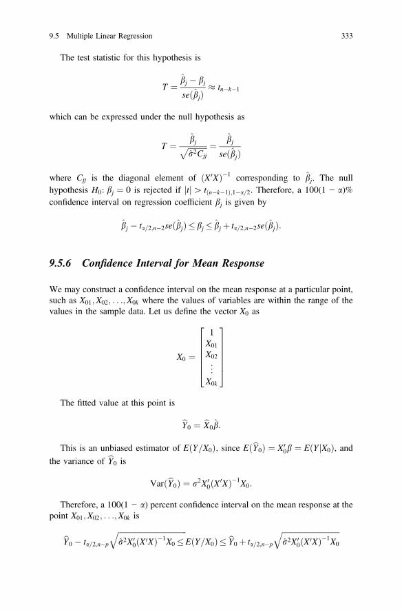
The test statistic for this hypothesis is
T ¼ bj � bj
seðbjÞ tn�k�1
which can be expressed under the null hypothesis as
T ¼ bjffiffiffiffiffiffiffiffiffiffir2Cjj
p ¼ bj
seðbjÞ
where Cjj is the diagonal element of ðX 0XÞ�1 corresponding to bj. The nullhypothesis H0: bj ¼ 0 is rejected if tj j[ tðn�k�1Þ;1�a=2. Therefore, a 100(1 − a)%confidence interval on regression coefficient bj is given by
bj � ta=2;n�2seðbjÞ� bj � bj þ ta=2;n�2seðbjÞ:
9.5.6 Confidence Interval for Mean Response
We may construct a confidence interval on the mean response at a particular point,such as X01;X02; . . .;X0k where the values of variables are within the range of thevalues in the sample data. Let us define the vector X0 as
X0 ¼
1X01
X02
..
.
X0k
2666664
3777775The fitted value at this point is
bY0 ¼ bX0b:
This is an unbiased estimator of EðY=X0Þ; since EðbY0Þ ¼ X 00b ¼ EðY X0j Þ, and
the variance of bY0 is
VarðbY0Þ ¼ r2X 00ðX 0XÞ�1X0:
Therefore, a 100(1 − a) percent confidence interval on the mean response at thepoint X01;X02; . . .;X0k is
bY0 � ta=2;n�p
ffiffiffiffiffiffiffiffiffiffiffiffiffiffiffiffiffiffiffiffiffiffiffiffiffiffiffiffiffiffiffiffiffiffiffiffir2X 0
0ðX 0XÞ�1X0 �q
EðY=X0Þ� bY0 þ ta=2;n�p
ffiffiffiffiffiffiffiffiffiffiffiffiffiffiffiffiffiffiffiffiffiffiffiffiffiffiffiffiffiffir2X 0
0ðX 0XÞ�1X0
q
9.5 Multiple Linear Regression 333

9.5.7 Prediction of New Observations
The regression model can be used to predict future observations on Y correspondingto particular values of the regressor variables, for example, XF1;XF2; . . .. . .;XFk. IfX 0F ¼ ½1;XF1;XF2; . . .. . .;XFk�, then a point estimate of the future observation YF at
the point XF1;XF2; . . .. . .;XFk is
bYF ¼ X 0F b:
A 100(1 − a) percent confidence interval for this future observation at the pointXF1;XF2; . . .;XFk is
bYF � tðn�k�1Þ;1�a=2
ffiffiffiffiffiffiffiffiffiffiffiffiffiffiffiffiffiffiffiffiffiffiffiffiffiffiffiffiffiffiffiffiffiffiffiffiffiffiffiffiffiffiffir2ð1þX 0
FðX 0XÞ�1XFÞq
� YFÞ
� bYF þ tðn�k�1Þ;1�a=2
ffiffiffiffiffiffiffiffiffiffiffiffiffiffiffiffiffiffiffiffiffiffiffiffiffiffiffiffiffiffiffiffiffiffiffiffiffiffiffiffiffiffiffir2ð1þX 0
FðX 0XÞ�1XFÞq
Example 9.7The data set used for this application is 5% random sample from the first wave ofthe Health and Retirement Study (HRS 2010). The outcome variable is weight (inkg) of the respondents and the independent variables are height (in cm), gender(male = 1, female = 0), sum of conditions (0, …, 5) ever had. The selected samplesize is 301.
In this example, a multiple linear regression model is fitted. The study wasconducted on elderly people. The outcome variable is weight (Y) and theexplanatory variables are height (X1), gender (X2, 1 for male and 0 for female), andnumber of health conditions ever had (X3). The regression model is
EðY X1;X2;X3Þ ¼ b0 þ b1X1 þ b2X2 þ b3X3j :
This model can be expressed in the following form too
Y ¼ b0 þ b1X1 þ b2X2 þ b3X3 þ e:
The least squares estimates of the parameters are
b0 ¼ �50:127; b1 ¼ 0:751; b2 ¼ �4:309 and b3 ¼ 1:123:
To test for the regression model, the null hypothesis is
H0: b1 ¼ b2 ¼ b3 ¼ 0
334 9 Correlation and Regression

and the alternative hypothesis can be stated as at least one of the regression coef-ficients is not zero. The analysis of variance table shows that the null hypothesis canbe rejected and there is evidence that one or more of the explanatory variables aresignificantly associated with weight of elderly people. The value of the test statistic,F, from the sample data is 49.357 (p-value < 0.001). The value of R2 is 0.333which implies that 33% of the total variation in the outcome variable can beexplained by the regression model considered in this example. Alternatively, it canbe said that two-thirds of the variation remains unexplained although the modelappears to be a statistically significant one. The search for the best possible modelneeds to be in the list of priorities to delineate possible strategies by a researcher.
As the overall model appears to be significant, we need to find the variables thatare significantly associated with weight of elderly people. The null and alternativehypotheses for testing the significance of three regression coefficients are(Table 9.10)
H01: b1 ¼ 0; H11: b1 6¼ 0;
H02: b2 ¼ 0; H12: b2 6¼ 0;
H03: b3 ¼ 0; H13 : b3 6¼ 0:
From the analysis of variance table, we observe that height is significantly andpositively associated (p-value < 0.001) with weight. Gender appears to have anegative association with weight, males demonstrate lower weight compared to
Table 9.10 Estimation and tests on the fit of multiple regression model for weight of elderlypeople
A. Coefficient of multiple determination
R R square Adjusted R square Std. error of the estimate Durbin–Watson
0.577 0.333 0.326 13.351 2.131
B. ANOVA table
Model Sum of squares df Mean square F Sig.
Regression 26393.106 3 8797.702 49.357 0.000
Residual 52938.618 297 178.245
Total 79331.724 300
C. Parameter estimates of multiple regression model
Model b t-value p-value
95.0% confidenceinterval for b
B Std.error
Lowerbound
Upperbound
Intercept −50.127 20.551 −2.439 0.015 −90.571 −9.683
Height 0.751 0.116 6.486 0.000 0.523 0.979
Gender −4.309 2.312 −1.864 0.063 −8.858 0.240
Number of conditionsever had
1.123 0.730 1.540 0.125 −0.313 2.559
9.5 Multiple Linear Regression 335
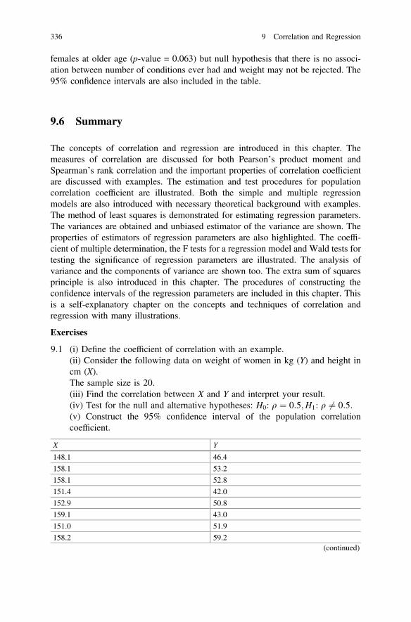
females at older age (p-value = 0.063) but null hypothesis that there is no associ-ation between number of conditions ever had and weight may not be rejected. The95% confidence intervals are also included in the table.
9.6 Summary
The concepts of correlation and regression are introduced in this chapter. Themeasures of correlation are discussed for both Pearson’s product moment andSpearman’s rank correlation and the important properties of correlation coefficientare discussed with examples. The estimation and test procedures for populationcorrelation coefficient are illustrated. Both the simple and multiple regressionmodels are also introduced with necessary theoretical background with examples.The method of least squares is demonstrated for estimating regression parameters.The variances are obtained and unbiased estimator of the variance are shown. Theproperties of estimators of regression parameters are also highlighted. The coeffi-cient of multiple determination, the F tests for a regression model and Wald tests fortesting the significance of regression parameters are illustrated. The analysis ofvariance and the components of variance are shown too. The extra sum of squaresprinciple is also introduced in this chapter. The procedures of constructing theconfidence intervals of the regression parameters are included in this chapter. Thisis a self-explanatory chapter on the concepts and techniques of correlation andregression with many illustrations.
Exercises
9:1 (i) Define the coefficient of correlation with an example.(ii) Consider the following data on weight of women in kg (Y) and height incm (X).The sample size is 20.(iii) Find the correlation between X and Y and interpret your result.(iv) Test for the null and alternative hypotheses: H0: q ¼ 0:5;H1: q 6¼ 0:5:(v) Construct the 95% confidence interval of the population correlationcoefficient.
X Y
148.1 46.4
158.1 53.2
158.1 52.8
151.4 42.0
152.9 50.8
159.1 43.0
151.0 51.9
158.2 59.2(continued)
336 9 Correlation and Regression
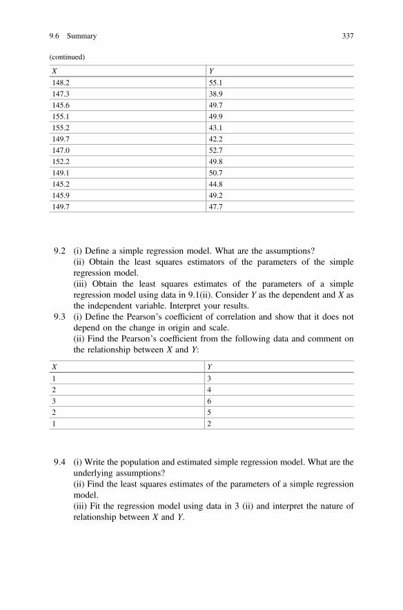
(continued)
X Y
148.2 55.1
147.3 38.9
145.6 49.7
155.1 49.9
155.2 43.1
149.7 42.2
147.0 52.7
152.2 49.8
149.1 50.7
145.2 44.8
145.9 49.2
149.7 47.7
9:2 (i) Define a simple regression model. What are the assumptions?(ii) Obtain the least squares estimators of the parameters of the simpleregression model.(iii) Obtain the least squares estimates of the parameters of a simpleregression model using data in 9.1(ii). Consider Y as the dependent and X asthe independent variable. Interpret your results.
9:3 (i) Define the Pearson’s coefficient of correlation and show that it does notdepend on the change in origin and scale.(ii) Find the Pearson’s coefficient from the following data and comment onthe relationship between X and Y:
X Y
1 3
2 4
3 6
2 5
1 2
9:4 (i) Write the population and estimated simple regression model. What are theunderlying assumptions?(ii) Find the least squares estimates of the parameters of a simple regressionmodel.(iii) Fit the regression model using data in 3 (ii) and interpret the nature ofrelationship between X and Y.
9.6 Summary 337
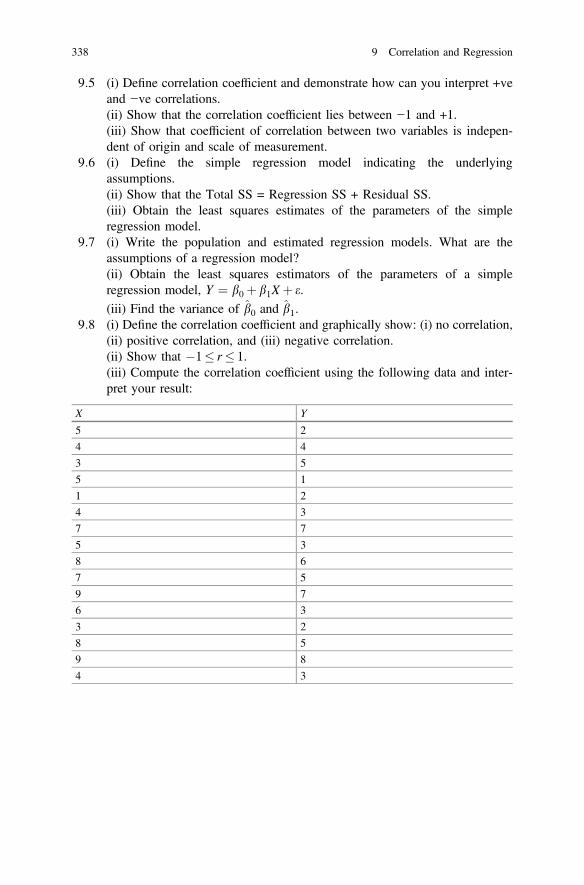
9:5 (i) Define correlation coefficient and demonstrate how can you interpret +veand −ve correlations.(ii) Show that the correlation coefficient lies between −1 and +1.(iii) Show that coefficient of correlation between two variables is indepen-dent of origin and scale of measurement.
9:6 (i) Define the simple regression model indicating the underlyingassumptions.(ii) Show that the Total SS = Regression SS + Residual SS.(iii) Obtain the least squares estimates of the parameters of the simpleregression model.
9:7 (i) Write the population and estimated regression models. What are theassumptions of a regression model?(ii) Obtain the least squares estimators of the parameters of a simpleregression model, Y ¼ b0 þ b1X þ e.(iii) Find the variance of b0 and b1.
9:8 (i) Define the correlation coefficient and graphically show: (i) no correlation,(ii) positive correlation, and (iii) negative correlation.(ii) Show that �1� r� 1.(iii) Compute the correlation coefficient using the following data and inter-pret your result:
X Y
5 2
4 4
3 5
5 1
1 2
4 3
7 7
5 3
8 6
7 5
9 7
6 3
3 2
8 5
9 8
4 3
338 9 Correlation and Regression
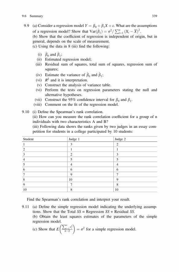
9:9 (a) Consider a regression model Y ¼ b0 þ b1X þ e. What are the assumptionsof a regression model? Show that Varðb1Þ ¼ r2=
Pni¼1 ðXi � XÞ2.
(b) Show that the coefficient of regression is independent of origin, but ingeneral, depends on the scale of measurement.(c) Using the data in 8 (iii) find the following:
(i) b0 and b1;(ii) Estimated regression model;(iii) Residual sum of squares, total sum of squares, regression sum of
squares;(iv) Estimate the variance of b0 and b1;(vi) R2 and it is interpretation.(v) Construct the analysis of variance table.(vi) Perform the tests on regression parameters stating the null and
alternative hypotheses.(vii) Construct the 95% confidence interval for b0 and b1.(viii) Comment on the fit of the regression model.
9:10 (i) Define the Spearman’s rank correlation.(ii) How can you measure the rank correlation coefficient for a group of nindividuals with two characteristics A and B?(iii) Following data shows the ranks given by two judges in an essay com-petition for students in a college participated by 10 students:
Student Judge 1 Judge 2
1 3 2
2 1 1
3 2 3
4 5 5
5 4 4
6 6 6
7 9 7
8 10 9
9 7 8
10 8 10
Find the Spearman’s rank correlation and interpret your result.
9:11 (a) Define the simple regression model indicating the underlying assump-tions. Show that the Total SS = Regression SS + Residual SS.(b) Obtain the least squares estimates of the parameters of the simpleregression model.
(c) Show that EPn
i¼1e2i
n�2
� �¼ r2 for a simple regression model.
9.6 Summary 339
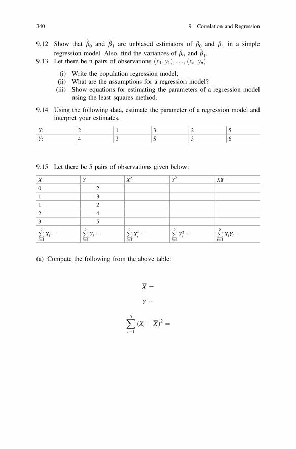
9:12 Show that b0 and b1 are unbiased estimators of b0 and b1 in a simpleregression model. Also, find the variances of b0 and b1.
9:13 Let there be n pairs of observations ðx1; y1Þ; . . .; ðxn; ynÞ(i) Write the population regression model;(ii) What are the assumptions for a regression model?(iii) Show equations for estimating the parameters of a regression model
using the least squares method.
9:14 Using the following data, estimate the parameter of a regression model andinterpret your estimates.
X: 2 1 3 2 5
Y: 4 3 5 3 6
9:15 Let there be 5 pairs of observations given below:
X Y X2 Y2 XY
0 2
1 3
1 2
2 4
3 5P5i¼1
Xi =P5i¼1
Yi =P5i¼1
X2
i =P5i¼1
Y2i =
P5i¼1
XiYi =
(a) Compute the following from the above table:
X ¼
Y ¼
X5i¼1
ðXi � XÞ2 ¼
340 9 Correlation and Regression

X5i¼1
ðYi � YÞ2 ¼
X5i¼1
ðXi � XÞðYi � YÞ ¼
(b) Calculate the Pearson’s correlation coefficient;(c) Interpret the correlation coefficient obtained in (a);(d) Is the correlation coefficient independent of
(i) change in origin?:(ii) change in scale?:
(e) Write the population regression model considering Y as the outcome variableand X as the explanatory variable;
(f) Write the estimated regression model;(g) Find the regression sum of squares and residual sum of squares.(h) Construct the analysis of variance table.(i) Perform tests on the parameters of the regression model.(j) Comment on your findings.
9:16 (a) For a regression model, Y ¼ Xbþ e, where X is ðn� ðkþ 1ÞÞ and b isðkþ 1Þ � 1 vector of parameters, then find the estimators of b.(b) Show that CovðbÞ ¼ ðX 0XÞ�1r2 for the above model.
9:17 Let us consider a model with k regressors, Y ¼ Xbþ e, where Y is n� 1, X isn� p, b is p� 1, and p = k + 1. If we partition b ¼ array�20lb1 � b2½ �,where b1 is ðp� rÞ � 1 and b2 is r � 1, then illustrate the test procedure forH0: b2 ¼ 0.
9:18 Briefly discuss the role of R2, adjusted R2, and residual mean square inselecting the best regression model.
9:19 Let us consider the following data on height (in cm), age (in months) andweight (in kg) of 25 children as shown below:
Age (X1) Height (X2) Weight (Y)
10 72.1 7.4
55 93.5 11.3
15 78.9 9.8
20 85.2 12.1
31 89.1 11.6(continued)
9.6 Summary 341
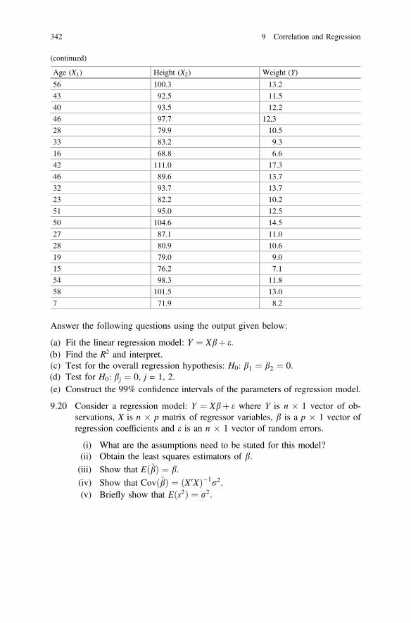
(continued)
Age (X1) Height (X2) Weight (Y)
56 100.3 13.2
43 92.5 11.5
40 93.5 12.2
46 97.7 12,3
28 79.9 10.5
33 83.2 9.3
16 68.8 6.6
42 111.0 17.3
46 89.6 13.7
32 93.7 13.7
23 82.2 10.2
51 95.0 12.5
50 104.6 14.5
27 87.1 11.0
28 80.9 10.6
19 79.0 9.0
15 76.2 7.1
54 98.3 11.8
58 101.5 13.0
7 71.9 8.2
Answer the following questions using the output given below:
(a) Fit the linear regression model: Y ¼ Xbþ e:(b) Find the R2 and interpret.(c) Test for the overall regression hypothesis: H0: b1 ¼ b2 ¼ 0.(d) Test for H0: bj ¼ 0, j = 1, 2.(e) Construct the 99% confidence intervals of the parameters of regression model.
9:20 Consider a regression model: Y ¼ Xbþ e where Y is n � 1 vector of ob-servations, X is n � p matrix of regressor variables, b is a p � 1 vector ofregression coefficients and e is an n � 1 vector of random errors.
(i) What are the assumptions need to be stated for this model?(ii) Obtain the least squares estimators of b.(iii) Show that EðbÞ ¼ b.(iv) Show that CovðbÞ ¼ ðX 0XÞ�1r2.(v) Briefly show that Eðs2Þ ¼ r2:
342 9 Correlation and Regression
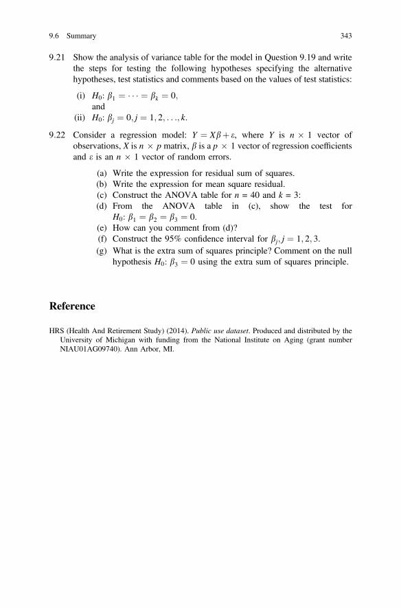
9:21 Show the analysis of variance table for the model in Question 9.19 and writethe steps for testing the following hypotheses specifying the alternativehypotheses, test statistics and comments based on the values of test statistics:
(i) H0: b1 ¼ ¼ bk ¼ 0;and
(ii) H0: bj ¼ 0; j ¼ 1; 2; . . .; k.
9:22 Consider a regression model: Y ¼ Xbþ e, where Y is n � 1 vector ofobservations, X is n � p matrix, b is a p � 1 vector of regression coefficientsand e is an n � 1 vector of random errors.
(a) Write the expression for residual sum of squares.(b) Write the expression for mean square residual.(c) Construct the ANOVA table for n = 40 and k = 3:(d) From the ANOVA table in (c), show the test for
H0: b1 ¼ b2 ¼ b3 ¼ 0.(e) How can you comment from (d)?(f) Construct the 95% confidence interval for bj; j ¼ 1; 2; 3.(g) What is the extra sum of squares principle? Comment on the null
hypothesis H0: b3 ¼ 0 using the extra sum of squares principle.
Reference
HRS (Health And Retirement Study) (2014). Public use dataset. Produced and distributed by theUniversity of Michigan with funding from the National Institute on Aging (grant numberNIAU01AG09740). Ann Arbor, MI.
9.6 Summary 343

Chapter 10Analysis of Variance
10.1 Introduction
The technique of analysis of variance (ANOVA) is used to compare several meansof several populations. It can be considered as a generalization of the t-test that isused for comparing two means from two populations.
For example, suppose that a researcher conducted a study to compare the effectsof four different types of medical training programs T1; T2; T3; and T4ð Þ on theattainment of students. In order to compare these training programs, the researcherselected 24 medical students in the same level of study and who obtained the samegrade in a placement test. Then, the researcher randomly divided these students intofour groups each with six students. After that, the researcher randomly applied eachtraining program on one of the four groups of students. In the end of the program,the researcher obtained the marks of the students (out of 15) which are summarizedin the following table:
Observations (marks)
Treatments Program T1ð Þ 11.6 7.3 11.4 11.0 8.6 9.2
Program T2ð Þ 6.2 8.1 9.8 5.1 7.0 8.6
Program T3ð Þ 11.9 8.1 12.6 14.2 10.7 11.4
Program T4ð Þ 10.5 15.0 11.8 13.7 14.7 12.8
One of the goals that the researcher wants to accomplish is to know whether real(or significant) differences exist between the means of the students’ marks for thedifferent programs. In other words, the researcher wants to know whether the typeof training program has an effect on the educational attainment measured by themarks of the students. In this example, and based on the ANOVA methodology, thetype of the training program is called the treatment factor (or independent variable),and the mark is called the response (or dependent variable) which is that quantitymeasured on the experimental units. The different training programs
© Springer Nature Singapore Pte Ltd. 2018M. A. Islam and A. Al-Shiha, Foundations of Biostatistics,https://doi.org/10.1007/978-981-10-8627-4_10
345

T1; T2; T3; and T4ð Þ are called the treatments or the levels of the factor, whereas astudent who receives one of the treatments and on which we measure the responseis called an experimental unit. The design of this kind of experiment is called thecompletely randomized design.
The existence of real differences between the means of marks for the differenttraining program indicates that the type of the training program has an effect on theeducational attainment of the students.
10.2 Completely Randomized Design: One-WayClassification
The completely randomized design (CRD) is one of the simplest and useful designs.In this design, we have one factor of interest that might have an effect on theresponse of interest. The response variable is denoted by Y. Suppose that thetreatment factor has a levels (or a treatments). Each level of the factor correspondsto a population. We select independent random samples of size n from the a pop-ulations; a sample from each population. Each population represents a level of thefactor; that is, each population represents a treatment.
The goal is to answer the following questions: Are all population means equal?Are some of them different? In other words, we need to answer the followingquestion: Does the factor significantly affect the response?
Statistically speaking, we need to test the following null and alternativehypotheses:
H0: l1 ¼ l2 ¼ � � � ¼ laH1: li 6¼ lj for some i and j;
where li is the mean of the ith population ði ¼ 1; 2; . . .; aÞ.Rejecting H0: l1 ¼ l2 ¼ � � � ¼ la indicates that there exist significant differ-
ences between the populations’ means, which means that there is a significant effectof the factor on the response. In this case, we wish to know which means aredifferent and to estimate the difference between the means.
10.2.1 Analysis of Variance Technique
The analysis of variance technique is based on partitioning the total variation in theobservations of the response variable into several components; each componentmeasures some source of variation.
346 10 Analysis of Variance
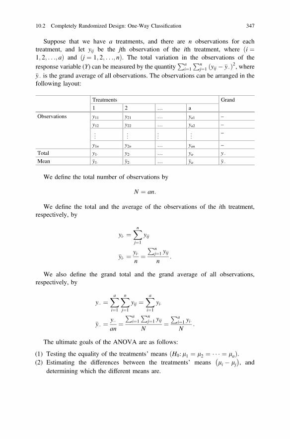
Suppose that we have a treatments, and there are n observations for eachtreatment, and let yij be the jth observation of the ith treatment, where ði ¼1; 2; . . .; aÞ and ðj ¼ 1; 2; . . .; nÞ. The total variation in the observations of theresponse variable (Y) can be measured by the quantity
Pai¼1
Pnj¼1 ðyij � �y��Þ2, where
�y�� is the grand average of all observations. The observations can be arranged in thefollowing layout:
Treatments Grand
1 2 … a
Observations y11 y21 … ya1 –
y12 y22 … ya2 –
..
. ... ..
. ... –
y1n y2n … yan –
Total y1� y2� … ya� y��Mean �y1� �y2� … �ya� �y��
We define the total number of observations by
N ¼ an:
We define the total and the average of the observations of the ith treatment,respectively, by
yi� ¼Xnj¼1
yij
�yi� ¼ yi�n¼
Pnj¼1 yijn
:
We also define the grand total and the grand average of all observations,respectively, by
y�� ¼Xai¼1
Xnj¼1
yij ¼Xai¼1
yi�
�y�� ¼ y��an
¼Pa
i¼1
Pnj¼1 yij
N¼
Pai¼1 yi�N
:
The ultimate goals of the ANOVA are as follows:
(1) Testing the equality of the treatments’ means H0: l1 ¼ l2 ¼ � � � ¼ lað Þ.(2) Estimating the differences between the treatments’ means li � lj
� �, and
determining which the different means are.
10.2 Completely Randomized Design: One-Way Classification 347

10.2.2 Decomposition of the Total Sum of Squares
As we mentioned earlier, the total variation in the observations as a whole can bemeasured by the corrected total sum of squares which is defined by
SSTOT ¼Xai¼1
Xnj¼1
ðyij � �y��Þ2:
The degrees of freedom associated with this sum of squares is
dfTOT ¼ an� 1 ¼ N � 1:
If we divide the corrected total sum of squares by its degrees of freedom, weobtain the ordinary sample variance of all observations, that is,
S2 ¼ SSTOTdfTOT
¼ SSTOTN � 1
¼Pa
i¼1
Pnj¼1 ðyij � �y��Þ2N � 1
:
This quantity is a measure of the total variation in all observations.There are two sources of the total variation which are as follows:
(1) The first kind of variation is due to the differences between the treatments.(2) The second kind of variation is due to the random error.
According to these two sources of variation, we can partition the total sum ofsquares SSTOT ¼ Pa
i¼1
Pnj¼1 ðyij � �y��Þ2 into two components which are as
follows:
(1) The treatment sum of squares (SSTRT):
This quantity measures the differences between the treatment means and definedby
SSTRT ¼ nXai¼1
ð�yi� � �y��Þ2:
The degrees of freedom associated with this sum of squares are
dfTRT ¼ a� 1:
Notice that the treatment sum of squares, SSTRT ¼ nPa
i¼1 ð�yi� � �y��Þ2, measuresthe sum of squares of the differences between the treatment averages �yi�ð Þ and thegrand average of the observations �y��ð Þ. A large value of SSTRT indicates theexistence of differences between the treatment’ means, consequently, we reject the
348 10 Analysis of Variance

hypothesis of the equality of the treatments’ means H0: l1 ¼ l2 ¼ � � � ¼ lað Þ forlarge values of SSTRT.
(2) The error sum of squares (SSE):
This quantity measures the differences between the observations within treat-ments and is defined by
SSE ¼Xai¼1
Xnj¼1
ðyij � �yi�Þ2
The degrees of freedom associated with this sum of squares are
dfE ¼ N � a:
Notice that the error sum of squares, SSE ¼ Pai¼1
Pnj¼1 ðyij � �yi�Þ2, measures the
sum of squares of the differences between the observations yij� �
and their average�yi�ð Þ within treatments.Algebraically, it can be shown that the total sum of squares,
SSTOT ¼ Pai¼1
Pnj¼1 ðyij � �y��Þ2, is the sum of two components; the first compo-
nent is (SSTRT) and the second component is (SSE). That is,
SSTOT ¼ SSTRTþ SSE
and equivalently, we may write
Xai¼1
Xnj¼1
ðyij � �y��Þ2 ¼ nXai¼1
ð�yi� � �y��Þ2 þXai¼1
Xnj¼1
ðyij � �yi�Þ2:
Similarly, we can partition the degrees of freedom associated with the total sumof squares dfTOT ¼ N � 1ð Þ into two components as follows:
dfTOT ¼ dfTRT þ dfE
and equivalently, we may write
N � 1 ¼ ða� 1Þþ ðN � aÞ:
10.2.3 Pooled Estimate of the Variance
Suppose that the observations of the ith treatment are
yi1; yi2; . . .; yin:
10.2 Completely Randomized Design: One-Way Classification 349

The sample variance of the observations of the ith treatment is
S2i ¼Pn
j¼1 ðyij � �yi�Þ2n� 1
:
This variance is associated with ðn� 1Þ degrees of freedoms. The pooled esti-mate of the variance using the sample variances of all treatments is
S2p ¼ðn� 1ÞS21 þðn� 1ÞS22 þ � � � þ ðn� 1ÞS2a
ðn� 1Þþ ðn� 1Þþ � � � þ ðn� 1Þ¼
Pai¼1 ðn� 1ÞS2iPai¼1 ðn� 1Þ
¼Pa
i¼1
Pnj¼1 ðyij � �yi�Þ2Pa
i¼1 ðn� 1Þ¼ SSE
N � a:
This quantity is called the mean square error (MSE).
Mean SquaresWhen we divide the sum of squares (SS) by its degrees of freedom (df), we obtainwhat is called mean square (MS), i.e.,
MS ¼ SSdf
:
We will define the following means of squares:
(1) The treatment mean square (MSTRT):This mean square is defined as follows:
MSTRT ¼ SSTRTdfTRT
¼ SSTRTa� 1
:
(2) The error mean square (MSE):This mean square is defined as follows:
MSE ¼ SSEdfE
¼ SSEN � a
:
As we mentioned earlier, the error mean square (MSE) is nothing but thepooled estimate of the variance, i.e., MSE ¼ S2p.
350 10 Analysis of Variance
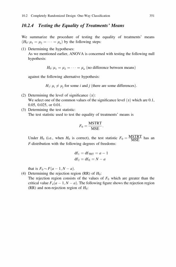
10.2.4 Testing the Equality of Treatments’ Means
We summarize the procedure of testing the equality of treatments’ meansH0: l1 ¼ l2 ¼ � � � ¼ lað Þ by the following steps:
(1) Determining the hypotheses:As we mentioned earlier, ANOVA is concerned with testing the following nullhypothesis:
H0:l1 ¼ l2 ¼ � � � ¼ la ðno difference between meansÞ
against the following alternative hypothesis:
H1: li 6¼ lj for some i and j ðthere are some differencesÞ:
(2) Determining the level of significance ðaÞ:We select one of the common values of the significance level ðaÞ which are 0.1,0.05, 0.025, or 0.01.
(3) Determining the test statistic:The test statistic used to test the equality of treatments’ means is
F0 ¼ MSTRTMSE
:
Under H0 (i.e., when H0 is correct), the test statistic F0 ¼ MSTRTMSE has an
F-distribution with the following degrees of freedoms:
df1 ¼ dfTRT ¼ a� 1
df2 ¼ dfE ¼ N � a
that is F0 �Fða� 1;N � aÞ.(4) Determining the rejection region (RR) of H0:
The rejection region consists of the values of F0 which are greater than thecritical value Faða� 1;N � aÞ. The following figure shows the rejection region(RR) and non-rejection region of H0:
10.2 Completely Randomized Design: One-Way Classification 351

(5) Determining the decision rule:We reject H0: l1 ¼ l2 ¼ � � � ¼ la at the significant level a if
F0 [ Faða� 1;N � aÞ:
ANOVA TableThe information needed to perform the ANOVA procedure is usually summarizedin so-called ANOVA table as follows:
Source ofvariation
Sum of squares Degreesoffreedom
Mean squares F-ratio F0ð Þ
Treatments(betweentreatments)
SSTRT ¼ nPa
i¼1 ð�yi� � �y��Þ2 a� 1 MSTRT ¼ SSTRTa�1 F0 ¼ MSTRT
MSE
Error (withintreatments)
SSE ¼Xa
i¼1
Xn
j¼1ðyij � �yi�Þ2
¼ SSTOT� SST
N � a MSE ¼ SSEN�a
Total SSTOT ¼ Pai¼1
Pnj¼1 ðyij � �y��Þ2 N � 1
Computational FormulasIn order to simplify calculating the sum of squares used in ANOVA table, we mayuse the following equivalent formulas:
SSTOT ¼Xai¼1
Xnj¼1
y2ij �y2��N
SSTRT ¼ 1n
Xai¼1
y2i� �y2��N
SSE ¼ SSTOT� SSTRT ðby subtractionÞ:
352 10 Analysis of Variance

The quantity y2��N is called the correction factor.
Example 10.1 A researcher wanted to compare the efficiency of four different typesof medical training programs T1; T2; T3; and T4ð Þ. In order to compare the effi-ciency of these training programs, the researcher selected 24 medical students in thesame level and who obtained the same grade in a placement test. Then, theresearcher randomly divided these students into four groups each with six students.After that, the researcher randomly applied each program on one of the four groupsof students. In the end of program, the researcher obtained the marks of the students(out of 15), which are summarized in the following table:
Observations (marks)
Treatments Program T1ð Þ 11.6 7.3 11.4 11.0 8.6 9.2
Program T2ð Þ 6.2 8.1 9.8 5.1 7.0 8.6
Program T3ð Þ 11.9 8.1 12.6 14.2 10.7 11.4
Program T4ð Þ 10.5 15.0 11.8 13.7 14.7 12.8
Do these data provide us with a sufficient evidence to conclude that there aresignificant differences among the training programs? In other words, does the typeof training program significantly affect the student attainment? Use a ¼ 0:05.
SolutionWe want to test H0: l1 ¼ l2 ¼ l3 ¼ l4ð Þ against H1: li 6¼ lj for some i and j
� �at
a ¼ 0:05.There are four treatments (programs): a ¼ 4.There are six observations in each sample: n ¼ 6.The total number of observation is N ¼ an ¼ 24.The following table summarizes the totals and the averages:
Treatments (programs) Grand
T1 T2 T3 T4Observations yij 11.6
7.311.411.08.69.2
6.28.19.85.17.08.6
11.98.112.614.210.711.4
10.515.011.813.714.712.8
–
–
–
–
–
Total yi�ð Þ 59.1 44.8 68.9 78.5 y�� ¼ 251:3
Average �yi�ð Þ 9.850 7.467 11.483 13.083 �y�� ¼ 10:471
10.2 Completely Randomized Design: One-Way Classification 353

In order to calculate the sums of squares, we first calculate the followingquantities:
y2��N
¼ ð251:3Þ224
¼ 2631:3204
Xai¼1
Xnj¼1
y2ij ¼ ð11:6Þ2 þ � � � þ ð12:8Þ2 ¼ 2800:65
Xai¼1
y2i� ¼ ð59:1Þ2 þð44:8Þ2 þð68:9Þ2 þð78:5Þ2 ¼ 16409:31:
Calculate the sums of squares (SS) using the calculating formulas:
SSTOT ¼Xai¼1
Xnj¼1
y2ij �y2��N
¼ 2800:65� 2631:3204 ¼ 169:3296
SSTRT ¼ 1n
Xai¼1
y2i� �y2��N
¼ 16ð16409:31Þ � 2631:3204 ¼ 103:5646
SSE ¼ SSTOT� SSTRT ¼ 169:3296� 103:5646 ¼ 65:765:
Calculate the degrees of freedoms (df):
dfTRT ¼ a� 1 ¼ 4� 1 ¼ 3
dfE ¼ N � a ¼ 24� 4 ¼ 20
dfTOT ¼ N � 1 ¼ 24� 1 ¼ 23:
Calculate the means of squares (MS):
MSTRT ¼ SSTRTa� 1
¼ 103:56464� 1
¼ 34:5215
MSE ¼ SSEN � a
¼ 65:76524� 4
¼ 3:2883:
We notice that the value of the treatment mean squares (MSTRT) is more thanten times as the value of the error mean squares (MSE), and this indicates that thetreatment means are likely to be different.
354 10 Analysis of Variance

Calculate the value of the test statistics F0ð Þ:
F0 ¼ MSTRTMSE
¼ 34:52153:2883
¼ 10:498:
Finding the critical Value Faða� 1;N � aÞð Þ:
F0:05ð3; 20Þ ¼ 3:10:
ANOVA TableWe summarize the above calculations in the following ANOVA table:
Source of variation Sum ofsquares
Degrees offreedom
Meansquares
F-ratioF0ð Þ
Treatments (betweentreatments)
103.5646 3 34.5215 10.498
Error (within treatments) 65.765 20 3.2883
Total 169.3296 23
DecisionSince F0 [F0:05ð3; 20Þ, we reject H0: l1 ¼ l2 ¼ l3 at the significance levela ¼ 0:05, and we conclude that the treatments’ means are significantly different,which mean that the type of the training program has an effect on the studentattainment.
10.2 Completely Randomized Design: One-Way Classification 355
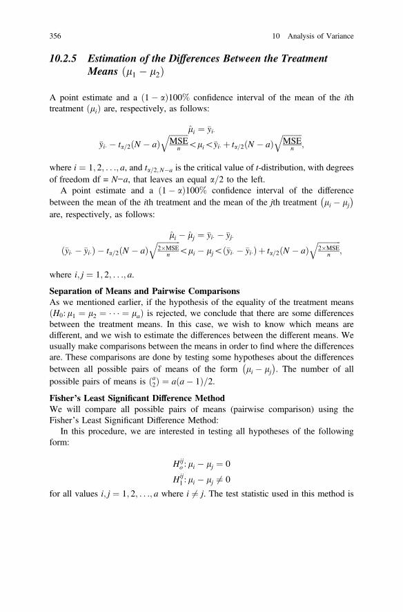
10.2.5 Estimation of the Differences Between the TreatmentMeans l1 � l2ð Þ
A point estimate and a ð1� aÞ100% confidence interval of the mean of the ithtreatment lið Þ are, respectively, as follows:
li ¼ �yi��yi� � ta=2ðN � aÞ
ffiffiffiffiffiffiffiffiffiffiMSE
n
q\li\�yi� þ ta=2ðN � aÞ
ffiffiffiffiffiffiffiffiffiffiMSE
n
q;
where i ¼ 1; 2; . . .; a, and ta=2;N�a is the critical value of t-distribution, with degreesof freedom df = N−a, that leaves an equal a=2 to the left.
A point estimate and a ð1� aÞ100% confidence interval of the differencebetween the mean of the ith treatment and the mean of the jth treatment li � lj
� �are, respectively, as follows:
li � lj ¼ �yi� � �yj�
ð�yi� � �yi�Þ � ta=2ðN � aÞffiffiffiffiffiffiffiffiffiffiffiffi2�MSE
n
q\li � lj\ð�yi� � �yi�Þ þ ta=2ðN � aÞ
ffiffiffiffiffiffiffiffiffiffiffiffi2�MSE
n
q;
where i; j ¼ 1; 2; . . .; a.
Separation of Means and Pairwise ComparisonsAs we mentioned earlier, if the hypothesis of the equality of the treatment meansH0: l1 ¼ l2 ¼ � � � ¼ lað Þ is rejected, we conclude that there are some differencesbetween the treatment means. In this case, we wish to know which means aredifferent, and we wish to estimate the differences between the different means. Weusually make comparisons between the means in order to find where the differencesare. These comparisons are done by testing some hypotheses about the differencesbetween all possible pairs of means of the form li � lj
� �. The number of all
possible pairs of means is ða2Þ ¼ aða� 1Þ=2.Fisher’s Least Significant Difference MethodWe will compare all possible pairs of means (pairwise comparison) using theFisher’s Least Significant Difference Method:
In this procedure, we are interested in testing all hypotheses of the followingform:
Hijo : li � lj ¼ 0
Hij1 : li � lj 6¼ 0
for all values i; j ¼ 1; 2; . . .; a where i 6¼ j. The test statistic used in this method is
356 10 Analysis of Variance

to ¼ �yi� � �yj�ffiffiffiffiffiffiffiffiffiffiffiffi2�MSE
n
q :
We reject Hijo : li ¼ lj if
toj j ¼ j �yi� � �yj�ffiffiffiffiffiffiffiffiffiffiffiffi2�MSE
n
q j [ ta2ðN � aÞ
which implies that
�yi� � �yj��� ��[ ta
2ðN � aÞ �
ffiffiffiffiffiffiffiffiffiffiffiffiffiffiffi2�MSE
n
r:
The quantity on the right-hand side of the last inequality is called the leastsignificant difference (LSD), i.e.,
LSD ¼ ta2ðN � aÞ �
ffiffiffiffiffiffiffiffiffiffiffiffiffiffiffi2�MSE
n
r:
Therefore, we reject Hijo : li ¼ lj if
�yi� � �yj��� ��[LSD:
Example 10.2 Consider the data in the previous example.
(1) Compare all possible pairs of means using a ¼ 0:05.(2) Construct 95% confidence intervals for the differences between all pairs of
means li � lj� �
.
Solution
(1) There are ða2Þ ¼ ð42Þ ¼ 6 possible pairs of means. The least significant difference(LSD) is
LSD ¼ ta2ðN � aÞ �
ffiffiffiffiffiffiffiffiffiffiffiffiffiffiffiffiffiffiffi2�MSE
n
r
¼ t0:025ð20Þ �ffiffiffiffiffiffiffiffiffiffiffiffiffiffiffiffiffiffiffiffiffiffi2� 3:2883
6
r
¼ 2:086� 1:0469
¼ 2:1839:
10.2 Completely Randomized Design: One-Way Classification 357

For any pair of means li; lj� �
, if �yi� � �yj��� ��[ 2:1839, we conclude that the
means li and lj are significantly different (i.e., we reject Hijo : li ¼ lj).
We summarize the calculations in the following table:
Pair of meansli;lj� � Absolute difference of the corresponding
averages �yi� � �yj��� �� Conclusion
l1;l2ð Þ �y1� � �y2�j j ¼ 9:85� 7:467j j ¼ 2:383 �y1� � �y2�j j[LSD(Significant)
l1;l3ð Þ �y1� � �y3�j j ¼ 9:85� 11:483j j ¼ 1:633 �y1� � �y3�j j\LSD
l1;l4ð Þ �y1� � �y4�j j ¼ 9:85� 13:083j j ¼ 3:233 �y1� � �y4�j j[LSD(Significant)
l2;l3ð Þ �y2� � �y3�j j ¼ 7467� 11:483j j ¼ 4:016 �y2� � �y3�j j[LSD(Significant)
l2;l4ð Þ �y2� � �y4�j j ¼ 7:467� 13:083j j ¼ 5:616 �y2� � �y4�j j[LSD(Significant)
ðl3;l4Þ �y3� � �y4�j j ¼ 11:483� 13:083j j ¼ 1:6 �y3� � �y4�j j\LSD
From this table, we notice that the mean of the second treatments l2ð Þ is sig-nificantly different from all other means.
(2) A 95% confidence interval for the difference li � lj� �
is
ð�yi� � �yi�Þ � ta=2ðN � aÞ �ffiffiffiffiffiffiffiffiffiffiffiffiffi2MSE
n
r
ð�yi� � �yi�Þ � t0:025ð20Þ �ffiffiffiffiffiffiffiffiffiffiffiffiffiffiffiffiffiffiffiffiffiffi2� 3:2883
6
r
ð�yi� � �yi�Þ � 2:086� 1:0469
ð�yi� � �yi�Þ � 2:1839:
We summarize the calculations in the following table:
Difference:li � lj
Point estimate:�yi� � �yi�
ð1� aÞ100% C.I. for li � lj� �
:ð�yi� � �yi�Þ � 2:1839
l1 � l2 2.383 0:199\l1 � l2\4:567
l1 � l3 −1.633 �3:817\l1 � l3\0:551
l1 � l4 −3.233 �5:417\l1 � l4\� 1:049
l2 � l3 −4.016 �6:200\l2 � l3\� 1:832
l2 � l4 −5.616 �7:800\l2 � l4\� 3:432
l3 � l4 −1.600 �3:784\l3 � l4\0:584
We noticed that all 95% confidence intervals involving the observations of theresponse variable into three componentsmean of the second treatment l2ð Þ do notcontain zero. Therefore, we conclude that l2 is different of all other means.
358 10 Analysis of Variance

10.3 Randomized Completely Block Design
The randomized completely block design (RCBD) is one of the most importantdesigns, and it is used in many applications. It can be considered as a generalizationof the paired t-test that used in comparing the means of two related populations.
It is used when the researcher wants to eliminate the effect of some controlledextraneous source of variation (called nuisance factor) from the comparisons of thetreatment means.
As we have seen, the completely randomized design is useful when the exper-imental units are homogenous. However, in many situations, it might be difficult tofind homogenous experimental units due to many practical reasons. In his case, wemay use the randomized completely block design in order to increase the precisionof the comparisons of the treatment means.
To show the usefulness of RCBD, suppose that in the previous exampledemonstrated in the last section, where the researcher wanted to compare the effi-ciency of four medical training programs, the students in the first and second groups(who received T1 and T2) were females, and the students in the third and fourthgroups (who received T3 and T4) were males. In this case, two factors are involvedin the design; the first factor is the type of program, whereas the second factor is thegender. The result of the ANOVA procedure of the CRD in the example showedthat there are significant differences between treatment means. Since there are twofactors involved, it is not clear in this situation which factor causes the differences.Indeed, the factor of interest is the type of program, whereas the gender is anuisance factor whose effect must be eliminated. The CRD fails to remove the effectof the gender on the treatment comparisons, since it affects the response (studentattainment) besides the factor of interest which is the type of program.
Another candidate nuisance factor in the previous example might be the study’slevel of the student. Suppose that students in the first group who received treatmentT1 were students at the bachelors’ level B1ð Þ, the students in the second group whoreceived treatment T2 were at the masters’ level B2ð Þ, the students in the third groupwho received treatment T3 were doctoral students B3ð Þ, and the students in thefourth group who received treatment T4 were postdoctoral students B4ð Þ, In thiscase, two factors are involved in the design; the first factor is the type of program,whereas the second factor is the level of study. The result of ANOVA procedure ofthe CRD in the example showed that there are significant differences betweentreatment means. Since there are two factors involved, it is not clear in this situationwhich factor causes the differences. Indeed, the factor of interest is the type ofprogram, whereas the level of study is a nuisance factor whose effect must beeliminated. The CRD fails to remove the effect of the level of study on the treatmentcomparisons, since it affects the response (student attainment) besides the factor ofinterest which is the type of program.
10.3 Randomized Completely Block Design 359

10.3.1 The Model and the Estimates of Parameters
An alternative design used when we want to remove the effect of a controllednuisance factor is the RCBD.
The RCBD is characterized by the following features:
1. We partition the experimental units into several blocks.2. The number of blocks must be equal to the number of different levels of the
nuisance factor. The nuisance factor is that factor we wish to eliminate its effectfrom the treatment comparisons.
3. Each block should contain homogenous experimental units.4. The number of experimental units in each block must be equal to the number of
treatments (number of different levels of the factor of interest).5. After forming the blocks, each treatment is randomly applied once and only
once in each block.6. Each treatment must appear in each block only one time.
The following figure illustrates the layout of the RCBD for the case in which wehave a treatments T1; T2; . . .; Tað Þ, and b blocks B1;B2; . . .;Bbð Þ:
It should be noticed that (1) the assignment of the treatments T1; T2; . . .; Tað Þ tothe experimental units inside each block must be done at random, and (2) eachtreatment must appear in each block only one time.
The analysis of variance in the RCBD is based on partitioning the total variationin the observations of the response variable into three components; each componentmeasures some source of variation.
Suppose that we have a treatments and b blocks, and let yij be the observation ofthe ith treatment in the jth block, where ði ¼ 1; 2; . . .; aÞ and ðj ¼ 1; 2; . . .; bÞ. Thetotal variation in the observations of the response variable (Y) can be measured bythe quantity SSTOT ¼ Pa
i¼1
Pbj¼1 ðyij � �y��Þ2, where �y�� is the grand average of all
360 10 Analysis of Variance

observations. The degrees of freedoms associated with this sum of squares isdfTOT ¼ ab� 1 ¼ N � 1.
The observations can be arranged in the following layout:
Blocks Treatment total Treatment average
1 2 … b
Treatments 1 y11 y12 … y1b y1� �y1�2 y21 y22 … y2b y2� �y2�
..
. ... ..
. ... ..
. ... ..
.
A ya1 ya2 … yab ya� �ya�Block total y�1 y�2 … y�b Grand Total ¼ y��Block average �y�1 �y�2 … �y�b Grand Average ¼ �y��
We define the total and the average of the observations of the ith treatment,respectively, by
yi� ¼Xbj¼1
yij
�yi� ¼ yi�b¼
Pbj¼1 yijb
We define the total and the average of the observations of the jth block,respectively, by
y�j ¼Xai¼1
yij
�y�j ¼ y�ja¼
Pai¼1 yija
:
We define the grand total and the grand average of all observations, respectively,by
y�� ¼Xai¼1
Xbj¼1
yij ¼Xai¼1
yi� ¼Xbj¼1
y�j
�y�� ¼ y��ab
¼Pa
i¼1
Pbj¼1 yij
N¼
Pai¼1 yi�N
¼Pb
j¼1 y�jN
:
We define the total number of observations by
10.3 Randomized Completely Block Design 361

N ¼ ab:
The goal of ANOVA in the RCBD is to test the equality of the treatments’means H0: l1 ¼ l2 ¼ � � � ¼ lað Þ after eliminating the effect of the nuisance factor.
In the RCBD, there are three sources of the total variation which are as follows:
(1) The first kind of variation is due to the differences between the treatments.(2) The second kind of variation is due to the differences between the blocks.(3) The third kind of variation is due to the random error.
According to these three sources of variation, we can partition the total sum ofsquares, SSTOT ¼ Pa
i¼1
Pbj¼1 ðyij � �y��Þ2, into three components which are as
follows:
(1) The treatment sum of squares (SSTRT):
SSTRT ¼ bXai¼1
ð�yi� � �y��Þ2
The degrees of freedom associated with this sum of squares are
dfTRT ¼ a� 1:
(2) The block sum of squares (SSBLK):
SSBLK ¼ aXbj¼1
ð�y�j � �y��Þ2:
The degrees of freedom associated with this sum of squares are
dfBLK ¼ b� 1:
(3) The error sum of squares (SSE):
SSE ¼Xai¼1
Xbj¼1
ðyij � �yi� � �y�j þ�y��Þ2:
The degrees of freedom associated with this sum of squares are
dfE ¼ ða� 1Þðb� 1Þ:
Algebraically, it can be shown that the total sum of squares, SSTOT ¼Pai¼1
Pbj¼1 ðyij � �y��Þ2 can be portioned into the sum of three components as
follows:
362 10 Analysis of Variance

SSTOT ¼ SSTRTþ SSBLKþ SSE
and equivalently, we may write
Xai¼1
Xbj¼1
ðyij � �y��Þ2 ¼ bXai¼1
ð�yi� � �y��Þ2 þ aXbj¼1
ð�y�j � �y��Þ2
þXai¼1
Xbj¼1
ðyij � �yi� � �y�j þ�y��Þ2:
Similarly, we can partition the degrees of freedom associated with the total sumof squares dfTOT ¼ ab� 1 ¼ N � 1ð Þ into three components as follows:
dfTOT ¼ dfTRT þ dfBLK þ dfE
and equivalently, we may write
ab� 1 ¼ ða� 1Þþ ðb� 1Þþ ða� 1Þðb� 1Þ:
For the RCBD, the relevant mean of squares is as follows:
(1) The treatment mean square (MSTRT) is
MSTRT ¼ SSTRTdfTRT
¼ SSTRTa� 1
:
(2) The block mean square (MSBLK) is
MSBLK ¼ SSBLKdfBLK
¼ SSBLKb� 1
:
(3) The error mean square (MSE) is
MSE ¼ SSEdfE
¼ SSEða� 1Þðb� 1Þ :
10.3.2 Testing the Equality of Treatment Means
The test statistic used to test the equality of treatments’ means H0: l1 ¼ l2 ¼� � � ¼ la is
10.3 Randomized Completely Block Design 363
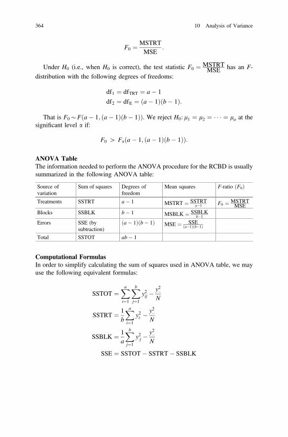
F0 ¼ MSTRTMSE
:
Under H0 (i.e., when H0 is correct), the test statistic F0 ¼ MSTRTMSE has an F-
distribution with the following degrees of freedoms:
df1 ¼ dfTRT ¼ a� 1
df2 ¼ dfE ¼ ða� 1Þðb� 1Þ:
That is F0 �Fða� 1; ða� 1Þðb� 1ÞÞ. We reject H0: l1 ¼ l2 ¼ � � � ¼ la at thesignificant level a if:
F0 [ Faða� 1; ða� 1Þðb� 1ÞÞ:
ANOVA TableThe information needed to perform the ANOVA procedure for the RCBD is usuallysummarized in the following ANOVA table:
Source ofvariation
Sum of squares Degrees offreedom
Mean squares F-ratio F0ð Þ
Treatments SSTRT a� 1 MSTRT ¼ SSTRTa�1 F0 ¼ MSTRT
MSEBlocks SSBLK b� 1 MSBLK ¼ SSBLK
b�1
Errors SSE (bysubtraction)
ða� 1Þðb� 1Þ MSE ¼ SSEða�1Þðb�1Þ
Total SSTOT ab� 1
Computational FormulasIn order to simplify calculating the sum of squares used in ANOVA table, we mayuse the following equivalent formulas:
SSTOT ¼Xai¼1
Xbj¼1
y2ij �y2��N
SSTRT ¼ 1b
Xai¼1
y2i� �y2��N
SSBLK ¼ 1a
Xbj¼1
y2�j �y2��N
SSE ¼ SSTOT� SSTRT � SSBLK
364 10 Analysis of Variance
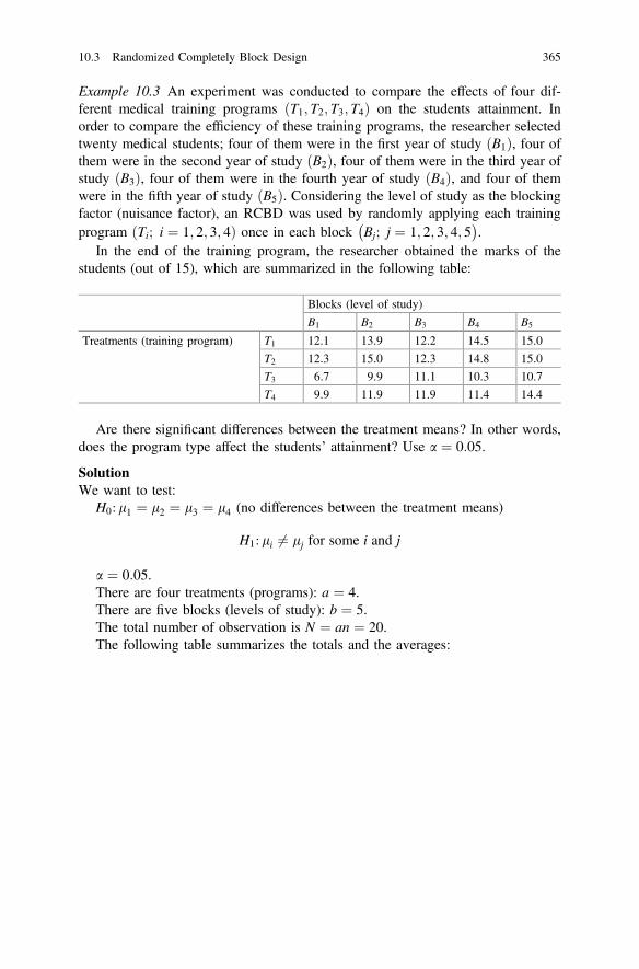
Example 10.3 An experiment was conducted to compare the effects of four dif-ferent medical training programs T1; T2; T3; T4ð Þ on the students attainment. Inorder to compare the efficiency of these training programs, the researcher selectedtwenty medical students; four of them were in the first year of study B1ð Þ, four ofthem were in the second year of study B2ð Þ, four of them were in the third year ofstudy B3ð Þ, four of them were in the fourth year of study B4ð Þ, and four of themwere in the fifth year of study B5ð Þ. Considering the level of study as the blockingfactor (nuisance factor), an RCBD was used by randomly applying each trainingprogram Ti; i ¼ 1; 2; 3; 4ð Þ once in each block Bj; j ¼ 1; 2; 3; 4; 5
� �.
In the end of the training program, the researcher obtained the marks of thestudents (out of 15), which are summarized in the following table:
Blocks (level of study)
B1 B2 B3 B4 B5
Treatments (training program) T1 12.1 13.9 12.2 14.5 15.0
T2 12.3 15.0 12.3 14.8 15.0
T3 6.7 9.9 11.1 10.3 10.7
T4 9.9 11.9 11.9 11.4 14.4
Are there significant differences between the treatment means? In other words,does the program type affect the students’ attainment? Use a ¼ 0:05.
SolutionWe want to test:
H0: l1 ¼ l2 ¼ l3 ¼ l4 (no differences between the treatment means)
H1: li 6¼ lj for some i and j
a ¼ 0:05.There are four treatments (programs): a ¼ 4.There are five blocks (levels of study): b ¼ 5.The total number of observation is N ¼ an ¼ 20.The following table summarizes the totals and the averages:
10.3 Randomized Completely Block Design 365

Blocks(level
ofstud
y)Treatment
total
Treatment
average
B1
B2
B3
B4
B5
Treatments(training
prog
ram)
T 112
.113
.912
.214
.515
.0y 1
�¼67:7
� y 1�¼
13:54
T 212
.315
.012
.314
.815
.0y 2
�¼69:4
� y 2�¼
13:88
T 36.7
9.9
11.1
10.3
10.7
y 3�¼
48:7
� y 3�¼
9:74
T 49.9
11.9
11.9
11.4
14.4
y 4�¼
59:5
� y 4�¼
11:9
Block
total
y �1¼
41:0
y �2¼
50:7
y �3¼
47:5
y �4¼
51:0
y �5¼
55:1
Grand
Total¼
y ��
¼24
5:3
Block
average
� y �1¼
10:25
� y �2¼
12:675
� y �3¼
11:875
� y �4¼
12:75
� y �5¼
13:775
Grand
Average
¼�y ��
¼12
:265
366 10 Analysis of Variance

In order to calculate the sums of squares, we first calculate the followingquantities:
y2��N
¼ ð245:3Þ220
¼ 3008:6045
Xai¼1
Xbj¼1
y2ij ¼ ð12:1Þ2 þ � � � þ ð14:4Þ2 ¼ 3100:57
Xai¼1
y2i� ¼ ð67:7Þ2 þð69:4Þ2 þð48:7Þ2 þð59:5Þ2 ¼ 15311:59
Xbj¼1
y2�j ¼ ð41:0Þ2 þð50:7Þ2 þð47:5Þ2 þð51:0Þ2 þð55:1Þ2 ¼ 12144:75:
Calculate the sums of squares (SS) using the calculating formulas:
SSTOT ¼Xai¼1
Xbj¼1
y2ij �y2��N
¼ 3100:57� 3008:6045 ¼ 91:9655
SSTRT ¼ 1b
Xai¼1
y2i� �y2��N
¼ 15ð15311:59Þ � 3008:6045 ¼ 53:7135
SSBLK ¼ 1a
Xbj¼1
y2�j �y2��N
¼ 14ð12144:75Þ � 3008:6045 ¼ 27:583
SSE ¼ SSTOT� SSTRT� SSBLK ¼ 91:9655� 53:7135� 27:583 ¼ 10:669:
Calculate the degrees of freedom (df):
dfTRT ¼ a� 1 ¼ 4� 1 ¼ 3
dfBLK ¼ b� 1 ¼ 5� 1 ¼ 4
dfE ¼ ða� 1Þðb� 1Þ ¼ 3� 4 ¼ 12
dfTOT ¼ N � 1 ¼ 20� 1 ¼ 19:
Calculate the means of squares (MS):
MSTRT ¼ SSTRTa� 1
¼ 53:71354� 1
¼ 17:9045
MSBLK ¼ SSBLKa� 1
¼ 27:5835� 1
¼ 6:8958
MSE ¼ SSEða� 1Þðb� 1Þ ¼
10:66912
¼ 0:8891:
We notice that the value of the treatment mean squares (MSTRT) is much higherthan the value of the error mean squares (MSE), and this indicates that the treatmentmeans are likely to be different.
10.3 Randomized Completely Block Design 367

Calculate the value of the test statistics F0ð Þ:
F0 ¼ MSTRTMSE
¼ 17:90450:8891
¼ 20:1378:
Finding the critical value Faða� 1; ða� 1Þðb� 1ÞÞð Þ:
F0:05ð3; 12Þ ¼ 3:49:
ANOVA TableWe summarize the above calculations in the following ANOVA table
Source ofvariation
Sum ofsquares
Degrees offreedom
Meansquares
F-ratioF0ð Þ
Treatments 53.7135 3 17.9045 20.1378
Blocks 27.583 4 6.8958
Error 10.669 12 0.8891
Total 91.9655 19
DecisionSince F0 [F0:05ð3; 12Þ, we reject H0: l1 ¼ l2 ¼ l3 ¼ l4 at the significance levela ¼ 0:05, and we conclude that the treatments’ means are significantly different,which mean that the type of the training program has an effect on the studentattainment.
10.4 Summary
The basic concepts and models of analysis of variance are introduced in thischapter. This chapter includes self-explanatory discussion on both one-way andtwo-way classifications. For both one-way and two-way analysis of variance, themodels and assumptions, the analysis of variance techniques, decomposition of
368 10 Analysis of Variance

total sum of squares, pooled estimate of variance, mean squares, and test for theequality of treatment means are discussed elaborately. The analysis of variancetables is shown. The computational techniques are illustrated with examples. Theestimation of the differences between the treatment means, separation of means, andpairwise comparisons are also illustrated in this chapter. The Fisher’s least signif-icant difference method is shown with example.
Exercises
10:1 The following hypothetical data represent the outcome of an experiment(temperature in degree Fahrenheit) with two different dose types ofmedicines (types A and B), and third type is a placebo (C) administeredrandomly to patients with high fever.Type of dose
A B C
100.2 101.5 102.3
101.3 100.3 103.1
100.4 99.8 102.6
102.5 102.3 102.4
101.5 101.5
102.7
(a) Write a suitable model that describes the variation in temperatureattributable to three different dose types of medicine. What are theassumptions?
(b) Perform the analysis of data and display the analysis of variance table.(c) Perform an appropriate test to determine whether there is variation in
body temperature due to three dose types of medicines.(d) Construct 95% one-sided and two-sided confidence intervals for the
difference between all pairs of mean temperatures.
10:2 In a study let us consider that four different procedures (A, B, C, and D) areapplied to randomly selected Type 2 diabetic subjects to find whether there isdifference in the mean performance in controlling their preprandial bloodglucose level (mmol/l).
A B C D
7.4 8.2 7.5 8.1
5.8 7.2 6.8 7.6
6.2 7.0 7.1 8.4
7.5 8.9 9.3 9.6
7.8 6.4 8.1 9.3
(a) Write a suitable analysis of variance model that describes the variationin blood glucose level due to different procedures. What are theassumptions?
10.4 Summary 369

(b) Analyze the data and summarize the results in an analysis of variancetable.
(c) Is there evidence in support of variation in preprandial blood glucoselevel? Perform an appropriate test and comment.
(d) Construct 95% two-sided confidence intervals for the differencebetween all pairs of mean blood glucose levels using a suitable leastsignificant difference method.
10:3 Consider that a study is performed on borderline high total cholesterol levelpatients (200–239 mg/dL) and three different treatment options are applied topatients living in three different communities.
City Treatment options
T1 T2 T3
City 1 204 223 227
203 212 228
190 212 207
City 2 215 214 215
178 203 206
200 204 204
City 3 213 213 217
178 193 207
190 194 206
(a) Write the appropriate analysis of variance model and indicate theunderlying assumptions.
(b) Find the treatment sum of squares, block sum of squares, and error sumof squares. What are the corresponding mean squares?
(c) How can you test the equality of treatment means? What is yourdecision?
(d) How can you test the equality of block means? What is your comment?(e) Interpret your overall findings.
10:4 The following data show outcomes of a study on seven different treatmentsapplied to three different groups (blocks) of people. In each group, treatmentswere assigned randomly. The outcomes, on a scale from 0 to 100, are dis-played below:
370 10 Analysis of Variance

Group Treatments
T1 T2 T3 T4 T5 T6 T7G1 75 77 68 69 93 74 43
82 80 70 73 81 78 53
77 81 72 75 88 76 62
G2 83 73 78 57 79 65 71
76 72 78 67 87 68 64
80 75 72 69 78 76 62
G3 87 77 78 63 86 75 64
78 73 75 67 79 71 65
81 77 69 79 82 70 55
(a) Write the appropriate analysis of variance model and indicate theunderlying assumptions.
(b) Find the treatment sum of squares, block sum of squares, and error sumof squares.
(c) How can you test the equality of treatment means? What is the teststatistic? Comment on the findings of the treatments from the study.
(d) How can you test the equality of block means? What is the test statistic?What is your comment?
(e) Interpret your overall findings.
10.4 Summary 371

Chapter 11Survival Analysis
11.1 Introduction
In this chapter, some important survival analysis techniques are introduced. Survivalanalysis deals with the time until occurrence of event of interest. We considersituations in which the analysis of times to the occurrence of events such as deathattributable to a certain cause, recovery from a disease, duration in disease-free statebefore recurrence of a disease, etc. are of interest. The time to the occurrence of anevent varies depending on the underlying risk or prognostic factors of the subjectsincluded in the study. Mathematically, one can think of time to event as merelymeaning a nonnegative valued variable. Although the term time to event is used forgeneral reference, other terms such as survival time and failure time will also befrequently used. The time to event refers to beginning to end (or the length orduration) prior to occurrence of an event. This requires a very well defined eventalong with the understanding through which that event may occur. To define therecurrence of a disease, for instance, we need to confirm the time of initiation of thedisease, duration of suffering from the disease before recovery at the first instance,duration of disease-free spell since recovery from the first spell before recurrence ofthe disease. In this case, the time to recurrence of disease is of interest. The startingtime is the time at recovery from the disease after first spell of the disease and the endpoint refers to the time at relapse of the disease indicating end of disease-free spell.
For collecting survival data, we may use the following basic study designs:
(a) Cohort Study,(b) Case-Control Study, and(c) Cross-sectional Study.
The first two types, cohort or follow-up and case-control or retrospective, areknown as longitudinal study designs. In a cohort/follow-up/prospective study, theindividuals are followed over time to observe incidence of disease as well as toobserve the changes in the status of disease. Here, the sampling is conducted on the
© Springer Nature Singapore Pte Ltd. 2018M. A. Islam and A. Al-Shiha, Foundations of Biostatistics,https://doi.org/10.1007/978-981-10-8627-4_11
373
basis of exposure status, and the incidence of the disease is observed at a subse-quent time for both the groups with or without exposure. This study design makes iteasier to study the natural history of a disease. On the other hand, if the associationbetween a factor and disease is based on information in the past, then the studydesign is called a case-control study design. In this design, the sampling is per-formed on the basis of disease status, instead of exposure status, and data onexposure status are collected from the past information provided by the respondentsfor both the groups with disease or without disease. The cross-sectional studydesigns are easier to conduct practically both in terms of cost and time because thedata on both exposure and disease status are collected at a particular point in time.However, it becomes difficult to assess whether there exists a time-dependentincidence of the disease as an effect of the hypothesized exposure from the datacollected by using a cross-sectional study design.
The survival analysis deals with human as the host and the forces within hostand environment that cause the events related to change in health conditions. One ofour major objectives is to explore the relationships between the host and envi-ronmental factors with state of health in a cause–effect framework. However, inmost of the cases, even if there is cause–effect relationship for certain events, thepresence of multiple causes and their interactive processes make it difficult toestablish the relationships using the data collected from various studies. The hostfactors include various personal traits termed as intrinsic factors. On the other hand,the environmental factors, classified by biological, social, and physical character-istics, are termed as extrinsic factors (Mausner and Kramer 1985). It is also note-worthy that the interrelations between host, agent, and environment, which may bein a broader sense considered as the interaction between host and environment dueto the presence of multiplicity of causes, need to be conceptualized in the studies ofsurvival analysis.
In a survival analysis study, the events are usually observed over time implyingthat some of the individuals may experience the event during the study period butothers may experience it later beyond the scope of the study resulting in incompleteobservations. These incomplete observations are called censoring. If we fix a pre-determined time to end the study, then an individual’s lifetime will be knownexactly only if it is less than some predetermined value. In such situations, the dataare said to be Type I (or time) censored. A Type II censored sample is one for whichonly the r smallest observations in a random sample of n items or subjects areobserved (1� r� n). Experiments involving Type II censoring are often used, forexample, in life testing; a total of n items is placed on test, but instead of continuinguntil all n items have failed, the test is terminated at the time of the rth item failure.Such tests can save time and money, since it could take a very long time for allitems to fail in some instances. If both event time and censoring time occur ran-domly, then it is called random censoring.
374 11 Survival Analysis

11.2 Some Measures of Association
One of the major concerns in a survival analysis study is to measure the extent andnature of association between the risk factor or exposure (E) and the disease (D).The measure of association usually involves a direct association between outcomeand exposure or study factor as well as a comparison between outcome andexposure with respect to a reference group which may not be considered as anexposure. That is why it becomes a challenge in many instances to measure theassociation with adequate epidemiologic reasoning. Let us consider that D denotesthe occurrence of disease and �D denotes nonoccurrence of the event. Similarly, letus denote E for presence of exposure and �E for absence of exposure. Then, we candisplay the bivariate frequency distribution for presence or absence of exposure andoccurrence or nonoccurrence of disease under three basic study designs:(i) prospective or cohort, (ii) retrospective or case-control, and (iii) cross-sectionalstudy design.
(i) Prospective Study: Under the prospective or cohort study designs, the incidenceof a disease can be measured for selected level of exposure or presence andabsence of the exposure over the study period. In this design, the role ofexposure level or presence and absence of exposure can be studied verycarefully, and the measure of association provided on the basis of a prospectivestudy may be considered as ideal for estimating measure of association. In aprospective study design, the fundamental condition of cause–effect is takeninto consideration, may not be in a very strict sense due to likely presence ofmultiple causes for an effect, but still provides a more specific measure ofassociation under given conditions in a relative sense. Mausner and Kramer(1985) observed that it is necessary to follow prospectively a defined group ofpeople and determine the rate at which new cases of disease occur to determineincidence.In Table 11.1, we follow up two groups with or without exposure and subse-quently note the disease status among the subjects belonging to exposed andnonexposed groups.
(ii) Case-Control Study: The prospective or cohort studies are always pre-ferred for studying the role of a specific exposure. However, it may not bea very practical study design if time and cost factors are involved. For aprospective study more time and costs are necessary and it is even moredifficult if the event of concern or the disease under study is rare. In that
Table 11.1 Table fordisplaying exposure anddisease status from aprospective study diseasestatus
Disease status
Exposure D �D Total
E a b a + b�E c d c + d
Total a + c b + d n
11.2 Some Measures of Association 375

case, the study needs to consider a very large number of subjects for ameaningful decision-making. Another important point is that for aprospective study, the setting up of specific hypothesis is of prime concernbecause the study is based on exposure status to determine its role indisease status. In addition, multiplicity of cause in explaining a diseasestatus makes the prospective study constrained. In case of the case-controlstudies, the cases and controls are selected on the basis of disease statusand the status regarding factors that might be considered as exposures arelooked for past exposures to factors. Then, Table 11.2 displays theexposure and disease status frequencies.
In Table 11.2 for case-control studies, the cases and controls are selected first andthe exposures are looked for retrospectively. In prospective study, the disease statusis observed longitudinally as outcomes of follow-up of exposed and nonexposedgroups of subjects. On the other hand, the approach is opposite in direction inrespect of time for a case-control study where cases and controls are selected asdisease status and their status in respect of exposures to factors are noted retro-spectively. It may be noted here that there may be ambiguity in the data fromretrospective studies about past events which may either be unavailable or may bemisreported.
For a matched case-control study, the frequencies are presented in the formatwhere matched pairs are considered (Table 11.3).
(iii) Cross-sectional Study: In a cross-sectional study, both risk factor orexposure and disease status are observed at the same time. These data arecollected generally by surveys. Although the cross-sectional studies areeasy to conduct and also less costly, the temporal sequence of events,necessary to establish a causal relationship, cannot be established due tolack of adequate information on occurrence of the disease and exposureto factors over time. The data from a cross-sectional study may onlyrepresent a snapshot view that represents the current status of both
Table 11.2 Table fordisplaying exposure anddisease status from acase-control study diseasestatus
Disease status
Exposure Case Control Total
E a b a + b�E c d c + d
Total a + c b + d n
Table 11.3 Table fordisplaying exposure anddisease status from a matchedcase-control study cases
Cases
Controls E �E Total
E a b a + b�E c d c + d
Total a + c b + d n
376 11 Survival Analysis

disease and exposure without providing any clue regarding the causalinference. However, these studies can be used to explore potential riskfactors.
Table 11.4 looks similar as the one for the prospective study but it has to beremembered that in case of a prospective study, the disease status is observed by afollow-up study for exposed and nonexposed groups. In a cross section study, weknow about disease and exposure to factors at the same time.
We can estimate the association between exposure and disease status using thefollowing measures referring the tables displayed above.
1. Relative Risk (RR) for Prospective Study: Relative risk shows the ratio of riskof incidence in the exposed group as compared to the risk of incidence in thenonexposed group. Here, the risks of incidence in the exposed and nonexposedgroups can be defined as follows:
Estimated risk of incidence for the exposed group = PðD Ej Þ ¼ aaþ b.
Estimated risk of incidence for the nonexposed group = PðD �Ej Þ ¼ ccþ d.
The estimated relative risk is
RR ¼ risk for exposed grouprisk for non-exposed group
¼ PðD Ej ÞPðD �EÞj
¼ a=ðaþ bÞc=ðcþ dÞ :
This measure is based on prospective study data. We cannot express the risks forincidence of disease from case-control or retrospective data.
Interpretation: If the relative risk,
(i) RR = 1, or ln RR = 0, then there is no association between exposure anddisease;
(ii) RR > 1, or ln RR > 0, then there is positive association between exposureand disease indicating higher risk of incidence for the exposed group ascompared to that of the nonexposed group;
(iii) RR < 1, or ln RR < 0, then there is protective association indicating lowerrisk of incidence in the exposed group as compared to that of the nonexposedgroup.
Table 11.4 Table fordisplaying exposure anddisease status from across-sectional study
Disease status
Exposure D �D Total
E a b a + b�E c d c + d
Total a + c b + d n
11.2 Some Measures of Association 377

Confidence Interval and Test for RRWe know that RR = 1 indicates no association between the exposure and diseasewhich is equivalent to testing for ln RR = 0. Let us show the test for the nullhypothesis H0: ln RR ¼ 0.
RR ¼ a=ðaþ bÞc=ðcþ dÞ and ln RR ¼ ln a
aþ b
� �� ln c
cþ d
� �.
It can be shown that the Varðln RRÞ ¼ b=ðaþ bÞa þ d=ðcþ dÞ
c .
Similarly, the seðln RRÞ ¼ffiffiffiffiffiffiffiffiffiffiffiffiffiffiffiffiffiffiffiffiffiffiffiffiffiffiffiffiffiffiffiffiffib=ðaþ bÞ
a þ d=ðcþ dÞc
q.
Assuming asymptotic normality, we can use the following test statistic
Z ¼ ln RR
seðln RRÞ ¼ln RRffiffiffiffiffiffiffiffiffiffiffiffiffiffiffiffiffiffiffiffiffiffiffiffiffiffiffiffiffiffiffiffiffi
b=ðaþ bÞa þ d=ðcþ dÞ
c
q �Nð0; 1Þ:
Acceptance of the null hypothesis indicates that the evidence from the sampledata is not sufficient to reject the null hypothesis of no association betweenexposure and disease, and rejection indicates a possible association.
For moderate or large sample, assuming normality, we can show that the 95%confidence limits for lnRR are
ln RR� 1:96 se ðln RRÞ;
which are ln RR� 1:96ffiffiffiffiffiffiffiffiffiffiffiffiffiffiffiffiffiffiffiffiffiffiffiffiffiffiffiffiffiffiffiffiffib=ðaþ bÞ
a þ d=ðcþ dÞc
q:
The 95% confidence limits for RR can be shown as
Lower Limit: RR e�1:96seðln RRÞ ¼ RR e�1:96ffiffiffiffiffiffiffiffiffiffiffiffiffiffiffiffiffiffiffiffiffiffiffib=ðaþ bÞ
a þ d=ðcþ dÞc
p.
Upper Limit: RR e1:96seðln RRÞ ¼ RR e1:96ffiffiffiffiffiffiffiffiffiffiffiffiffiffiffiffiffiffiffiffiffiffiffib=ðaþ bÞ
a þ d=ðcþ dÞc
p.
2. Risk Odds Ratio (ROR): A more convenient and popular measure for mea-suring the association between occurrence of disease in the exposed and non-exposed groups is the odds ratio. The odds ratio summarizes the ratio of odds ofincidence of disease to non-disease in the exposed group with that of thenonexposed group. The risk odds ratio is defined as
ROR ¼ PðD Ej Þ=½1� PðD EÞ�jPðD �EÞ=½1� PðD �EÞ�jj ;
where the odds of disease in the exposed group are in the numerator and the odds ofdisease in the nonexposed group are in the denominator. This is popularly known asthe odds ratio or OR. For two independent groups by exposure status, the condi-tional probabilities represent the probabilities of number of incidence cases in the
378 11 Survival Analysis

exposed and nonexposed groups. The probability distributions of number of casesin the exposed and nonexposed groups are binomial distributions with parametersaþ b;PðD EÞjð Þ and cþ d;PðD �EÞjð Þ, respectively.The estimates of PðD Ej Þ and PðD �Ej Þ are
PðD Ej Þ ¼ aaþ b
and PðD �Ej Þ ¼ ccþ d
:
We can also show that
1� PðD Ej Þ ¼ 1� aaþ b
¼ baþ b
and 1� PðD �Ej Þ ¼ 1� ccþ d
¼ dcþ d
:
Hence, the estimator of the OR can be shown as
OR ¼ PðD Ej Þ=½1� PðD EÞ�jPðD �EÞ=½1� PðD �EÞ�j�� :
The variances of PðD Ej Þ and PðD �Ej Þ are
Var ½PðD EÞ�j ¼ ½PðD EÞ�j ½1� PðD EÞ�jðaþ cÞ ; and
Var ½PðD �EÞ�j ¼ ½PðD �EÞ�j ½1� PðD �EÞ�jðbþ dÞ :
Then taking logarithm of OR, we find
lnOR ¼ ln PðD Ej Þ=½1� PðD EÞ�j� �� ln PðD �Ej Þ=½1� PðD �EÞ�j� �;
where the first term is a function of the proportion of disease cases in the exposedgroup which is the familiar odds for the exposed group, and the second term is afunction of the proportion of disease cases in the nonexposed group which is theodds for the nonexposed group. We can obtain the variance of the odds for both theexposed and nonexposed groups using the delta method as shown below:
11.2 Some Measures of Association 379

Var lnOR� � ¼ Var ln PðD Ej Þ=½1� PðD EÞ�j� � �þVar ln PðD �Ej Þ=½1� PðD �EÞ�j� � �
¼ 1PðD Ej Þ þ
1½1� PðD EÞ�j
�2Var PðD Ej Þ� �
þ 1PðD �Ej Þ þ
1½1� PðD �EÞ�j
�2Var PðD �Ej Þ� �
¼ 1PðD Ej Þ þ
1½1� PðD EÞ�j
�2PðD Ej Þ½1� PðD Ej Þ�ðaþ bÞ
þ 1PðD �Ej Þ þ
1½1� PðD �EÞ�j
�2PðD �Ej Þ½1� PðD �Ej Þ�ðcþ dÞ
¼ 1ðaþ bÞ PðD Ej Þ=½1� PðD EÞ�jf g þ 1
ðcþ dÞ PðD �Ej Þ=½1� PðD �EÞ�jf g :
The estimate of the variance of lnOR is
Var ln OR� � ¼ 1
ðaþ bÞ PðD Ej Þ=½1� PðD EÞ�j� þ 1
ðcþ dÞ PðD �Ej Þ=½1� PðD �EÞ�j� :This can be rewritten as
Var ln OR� � ¼ 1
ðaþ bÞ aðaþ bÞ � b
ðaþ bÞn o þ 1
ðcþ dÞ cðcþ dÞ � b
ðcþ dÞn o
¼ 1aþ 1
bþ 1
cþ 1
d:
We can now obtain the estimate of the variance of OR
Var OR� � ¼ OR
2 1aþ 1
bþ 1
cþ 1
d
� :
The estimate of the standard error of OR is
se OR� � ¼ OR
ffiffiffiffiffiffiffiffiffiffiffiffiffiffiffiffiffiffiffiffiffiffiffiffiffiffiffiffiffiffiffiffiffiffiffiffiffiffi1aþ 1
bþ 1
cþ 1
d
� s:
Interpretation: The interpretation of an odds ratio is similar to that of the relativerisk as stated below:
(i) OR = 1 or ln OR = 0 shows that there is no association between exposureand disease;
380 11 Survival Analysis

(ii) OR > 1, or ln OR > 0 shows that there is positive association betweenexposure and disease indicating higher risk of incidence for the exposedgroup as compared to that of the nonexposed group;
(iii) OR < 1, or ln OR < 0 shows that there is protective association indicatinglower risk of incidence in the exposed group as compared to that of thenonexposed group.
Confidence Interval and Test for ORWe know that OR = 1 indicates no association between the exposure and diseasewhich is equivalent to testing for ln OR = 0. Let us show the test for the nullhypothesis H0: ln OR ¼ 0.
OR ¼ adbc and lnOR ¼ ln að Þ � ln bð Þ � ln cð Þþ lnðdÞ:
It can be shown that the Varðln ORÞ ¼ 1a þ 1
b þ 1c þ 1
d :
Similarly, the seðln ORÞ ¼ffiffiffiffiffiffiffiffiffiffiffiffiffiffiffiffiffiffiffiffiffiffiffiffiffiffiffiffi1a þ 1
b þ 1c þ 1
d
q.
Assuming asymptotic normality for large sample size, we can use the followingtest statistic:
Z ¼ ln OR
seðln ORÞ ¼ln ORffiffiffiffiffiffiffiffiffiffiffiffiffiffiffiffiffiffiffiffiffiffiffiffiffiffiffiffi
1a þ 1
b þ 1c þ 1
d
q �Nð0; 1Þ:
Non-rejection of null hypothesis indicates that there is not sufficient evidencefrom the sample data in favor of rejecting the null hypothesis of no associationbetween exposure and disease and rejection indicates possible association.
For moderate or large sample, assuming normality, we can show that the 95%confidence limits for lnOR are
lnOR� 1:96 seðln ORÞ;
which are lnOR� 1:96ffiffiffiffiffiffiffiffiffiffiffiffiffiffiffiffiffiffiffiffiffiffiffiffiffiffiffiffi1a þ 1
b þ 1c þ 1
d
q:
The 95% confidence limits for OR can be shown as
Lower Limit: OR e�1:96seðln ORÞ ¼ OR e�1:96ffiffiffiffiffiffiffiffiffiffiffiffiffiffiffiffiffi1aþ 1
bþ 1cþ 1
d
p.
Upper Limit: OR e1:96seðlnORÞ ¼ OR e1:96ffiffiffiffiffiffiffiffiffiffiffiffiffiffiffiffiffi1aþ 1
bþ 1cþ 1
d
p.
3. Risk Ratio for Case-Control Study
The case-control study is retrospective over time and the study is conductedamong cases and controls to find the exposure to factor in the past which mighthave caused the disease. Two essential risks or probabilities for obtaining risk ratio,
11.2 Some Measures of Association 381
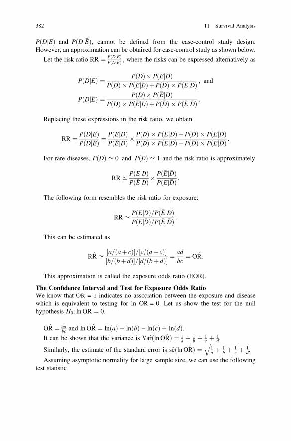
PðD EÞ and PðD �EÞjj , cannot be defined from the case-control study design.However, an approximation can be obtained for case-control study as shown below.
Let the risk ratio RR ¼ PðD EÞjPðD �EÞj ; where the risks can be expressed alternatively as
PðD Ej Þ ¼ PðDÞ � PðE DÞjPðDÞ � PðE DÞþPð�DÞ � PðE �DÞjj ; and
PðD �Ej Þ ¼ PðDÞ � Pð�E DÞjPðDÞ � Pð�E DÞþPð�DÞ � Pð�E �DÞjj :
Replacing these expressions in the risk ratio, we obtain
RR ¼ PðD EÞjPðD �EÞj ¼ PðE DÞj
Pð�E DÞj � PðDÞ � Pð�E DÞþPð�DÞ � Pð�E �DÞjjPðDÞ � PðE DÞþPð�DÞ � PðE �DÞjj :
For rare diseases, PðDÞ ’ 0 and Pð�DÞ ’ 1 and the risk ratio is approximately
RR ’ PðE DÞjPð�E DÞj � Pð�E �DÞj
PðE �DÞj :
The following form resembles the risk ratio for exposure:
RR ’ PðE DÞ=j Pð�E DÞjPðE �DÞ=Pð�E �DÞjj :
This can be estimated as
RR ’ ½a=ðaþ cÞ�=½c=ðaþ cÞ�½b=ðbþ dÞ�=½d=ðbþ dÞ� ¼
adbc
¼ OR:
This approximation is called the exposure odds ratio (EOR).
The Confidence Interval and Test for Exposure Odds RatioWe know that OR = 1 indicates no association between the exposure and diseasewhich is equivalent to testing for ln OR = 0. Let us show the test for the nullhypothesis H0: ln OR ¼ 0.
OR ¼ adbc and lnOR ¼ ln að Þ � ln bð Þ � ln cð Þþ lnðdÞ.
It can be shown that the variance is Varðln ORÞ ¼ 1a þ 1
b þ 1c þ 1
d.
Similarly, the estimate of the standard error is seðln ORÞ ¼ffiffiffiffiffiffiffiffiffiffiffiffiffiffiffiffiffiffiffiffiffiffiffiffiffiffiffiffi1a þ 1
b þ 1c þ 1
d
q.
Assuming asymptotic normality for large sample size, we can use the followingtest statistic
382 11 Survival Analysis

Z ¼ ln OR
seðln ORÞ ¼ln ORffiffiffiffiffiffiffiffiffiffiffiffiffiffiffiffiffiffiffiffiffiffiffiffiffiffiffiffi
1a þ 1
b þ 1c þ 1
d
q �Nð0; 1Þ:
Non-rejection of null hypothesis indicates that there is not sufficient evidencefrom the sample data in favor of rejecting the null hypothesis of no associationbetween exposure and disease and rejection indicates possible association betweenexposure and disease status.
For moderate or large sample, assuming normality, we can show that the 95%confidence limits for ln OR are
lnOR� 1:96 se ðln ORÞ;
which are lnOR� 1:96ffiffiffiffiffiffiffiffiffiffiffiffiffiffiffiffiffiffiffiffiffiffiffiffiffiffiffiffi1a þ 1
b þ 1c þ 1
d
q:
The 95% confidence limits for OR can be shown as
Lower Limit: OR e�1:96seðln ORÞ ¼ OR e�1:96ffiffiffiffiffiffiffiffiffiffiffiffiffiffiffiffiffi1aþ 1
bþ 1cþ 1
d
p.
Upper Limit: OR e1:96seðlnORÞ ¼ OR e1:96ffiffiffiffiffiffiffiffiffiffiffiffiffiffiffiffiffi1aþ 1
bþ 1cþ 1
d
p.
4. Odds Ratio from Cross-Sectional Data
Despite serious limitations of the odds ratio from a cross-sectional study design,we still use it as a measure of prevalence odds ratio. These limitations are welldocumented in the literature but still, the need for cross-sectional study designs issometimes necessary to provide quick understanding about the potential relation-ships between exposure and disease. A careful attention is to be given to thelimitations of such findings though.
The estimated probabilities can be obtained from cross-sectional cell frequenciesfor exposure status and disease status. The estimated probabilities, using the cellfrequencies shown in Table 11.4, are presented.
The estimated probabilities are (Table 11.5)
p11 ¼ an; p10 ¼ b
n; p01 ¼ c
n; p10 ¼ d
n:
Table 11.5 Probabilities ofexposure and disease statusfrom a cross-sectional study
Exposure status Disease status
D �D Total
E p11 p10 p1:�E p01 p00 p0:Total p:1 p:0 1
11.2 Some Measures of Association 383

Similarly, the marginal probabilities for exposure status arep1: ¼ aþ b
n and p0: ¼ cþ dn :
The odds for presence or absence of exposure may be defined as
OE ¼ PðD EÞjPð�D EÞj ¼ p11=p1:
p10=p1:¼ a
b;
and
O�E ¼ PðD �EÞjPð�D �EÞj ¼ p01=p0:
p00=p0:¼ c
d:
The odds ratio is
OR ¼ OE
O�E
¼ a=bc=d
¼ adbc
:
The variance of the estimator of odds ratio can be shown by using the multi-nomial distribution and using the delta method it can be shown that
Var ln OR� � ¼ 1
aþ 1
bþ 1
cþ 1
d:
Confidence Interval and Test for ORThe null hypothesis is H0: ln OR ¼ 0.
Assuming asymptotic normality for large sample size, we can use the followingtest statistic:
Z ¼ ln OR
seðln ORÞ ¼ln ORffiffiffiffiffiffiffiffiffiffiffiffiffiffiffiffiffiffiffiffiffiffiffiffiffiffiffiffi
1a þ 1
b þ 1c þ 1
d
q �Nð0; 1Þ:
The 95% confidence limits for lnOR are
lnOR� 1:96 seðln ORÞ;
which are lnOR� 1:96ffiffiffiffiffiffiffiffiffiffiffiffiffiffiffiffiffiffiffiffiffiffiffiffiffiffiffiffi1a þ 1
b þ 1c þ 1
d
q.
It can also be shown that 95% confidence limits for OR can be shown as
Lower Limit: OR e�1:96seðln ORÞ ¼ OR e�1:96ffiffiffiffiffiffiffiffiffiffiffiffiffiffiffiffiffi1aþ 1
bþ 1cþ 1
d
p:
Upper Limit: OR e1:96seðlnORÞ ¼ OR e1:96ffiffiffiffiffiffiffiffiffiffiffiffiffiffiffiffiffi1aþ 1
bþ 1cþ 1
d
p:
Example 11.1 Let us consider a hypothetical example on incidence of a diseaseamong the infants with low and normal birth weight from a prospective study
384 11 Survival Analysis

continued for one year on the newly born babies in a community. The data arepresented in Table 11.6.
In this example, low birth weight is an exposure and normal birth weight isconsidered as nonexposed for the incidence of disease being studied. The estimateof relative risk is obtained from the ratio of the risks for the exposed and nonex-posed groups as follows:
Estimate of risk for the low birthweight group ¼ aaþ b
¼ 60600
¼ 0:1000; and
Estimate of risk for the normal group ¼ ccþ d
¼ 501950
¼ 0:0256:
The estimate of the relative risk is
RR ¼ RE
R�E¼ 0:1
0:0256¼ 3:9062:
The estimate of the relative risk shows that the risk of disease for low birthweight babies is about 3.91 times higher than the risk for normal birth weightbabies.
To test for the statistical significance of no association between birth weight andthe disease, the null hypothesis is H0: ln RR ¼ 0.
The estimate of log relative risk is
ln RR ¼ lna
aþ b
� � ln
ccþ d
� ¼ �2:3026� ð�3:6652Þ ¼ 1:3626:
The estimate of the standard error of the log relative risk is
seðln RRÞ ¼ffiffiffiffiffiffiffiffiffiffiffiffiffiffiffiffiffiffiffiffiffiffiffiffiffiffiffiffiffiffiffiffiffiffi540=600
60 þ 1950=200050
q¼ ffiffiffiffiffiffiffiffiffiffiffiffiffiffiffiffiffiffiffiffiffiffiffiffiffiffiffiffiffiffi
0:015þ 0:0195p ¼ 0:1857:
The test statistic for large sample size is
Z ¼ ln RR
seðln RRÞ ¼ln RRffiffiffiffiffiffiffiffiffiffiffiffiffiffiffiffiffiffiffiffiffiffiffiffiffiffiffiffiffiffiffiffiffi
b=ðaþ bÞa þ d=ðcþ dÞ
c
q �Nð0; 1Þ
and for the sample data, the test statistic value can be computed
Table 11.6 Table fordisplaying hypothetical dataon birth weight and diseasestatus from a prospectivestudy
Disease status
Birth weight D �D Total
Low 60 540 600
Normal 50 1950 2000
Total 110 2490 2600
11.2 Some Measures of Association 385
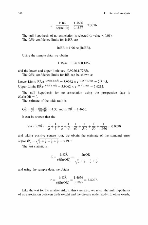
z ¼ ln RR
seðln RRÞ ¼1:36260:1857
¼ 7:3376:
The null hypothesis of no association is rejected (p-value < 0.01).The 95% confidence limits for ln RR are
ln RR� 1:96 se ðln RRÞ:
Using the sample data, we obtain
1:3626� 1:96� 0:1857
and the lower and upper limits are (0.9986,1.7265).The 95% confidence limits for RR can be shown as
Lower Limit: RR e�1:96seðln RRÞ ¼ 3:9062� e�1:96�1:3626 ¼ 2:7145.
Upper Limit: RR e1:96seðln RRÞ ¼ 3:9062� e1:96�1:3626 ¼ 5:6212:
The null hypothesis for no association using the prospective data isH0: ln OR ¼ 0.
The estimate of the odds ratio is
OR ¼ adbc ¼ 60�1950
540�50 ¼ 4:33 and lnOR ¼ 1:4656.
It can be shown that the
Var ðln ORÞ ¼ 1aþ 1
bþ 1
cþ 1
d¼ 1
60þ 1
540þ 1
50þ 1
1950¼ 0:0390
and taking positive square root, we obtain the estimate of the standard error
seðln ORÞ ¼ffiffiffiffiffiffiffiffiffiffiffiffiffiffiffiffiffiffiffiffiffiffiffiffiffiffiffiffi1a þ 1
b þ 1c þ 1
d
q¼ 0:1975:
The test statistic is
Z ¼ ln OR
seðln ORÞ ¼ln ORffiffiffiffiffiffiffiffiffiffiffiffiffiffiffiffiffiffiffiffiffiffiffiffiffiffiffiffi
1a þ 1
b þ 1c þ 1
d
q
and using the sample data, we obtain
z ¼ ln OR
seðln ORÞ ¼1:46560:1975
¼ 7:4207:
Like the test for the relative risk, in this case also, we reject the null hypothesisof no association between birth weight and the disease under study. In other words,
386 11 Survival Analysis

there is evidence in support of rejection of the null hypothesis of no associationbetween birth weight of babies and disease status.
The 95% confidence limits for ln OR are
lnOR� 1:96 se ðln ORÞ
and using the sample data, we obtain the lower and upper limits from
1:4656� 1:96� 0:1975
which are (1.0785, 1.8527).We can construct the 95% confidence limits for OR can be shown as
Lower Limit: OR e�1:96seðln ORÞ ¼ 4:33� e�1:96�0:1975 ¼ 2:9402.
Upper Limit: OR e1:96seðlnORÞ ¼ 4:33� e1:96�0:1975 ¼ 6:3768:
11.3 Nonparametric Estimation
There are two different types of nonparametric methods extensively used fornonparametric estimation of survival function, S(t). These are (i) the actuarialmethod and (ii) the product-limit or Kaplan–Meier method. First one is used mostlyin actuarial science and the second method in both epidemiology and survivalanalysis in addition to extensive use in other fields as well. In this section, theactuarial method of constructing a life table and the product-limit method arediscussed.
The Actuarial MethodLet time be partitioned into a fixed sequence of intervals I1, I2, …kIk. Theseintervals may or may not be of equal lengths, although mostly they are of equallengths. We can show the intervals as follows:
1 I 2
I k
0 t1 t 2 …………….. t 1−k t k
For a life table let us define the following:
ni = number alive at the beginning of Ii,di = number of deaths during Ii,li = number lost to follow-up during Ii,
11.2 Some Measures of Association 387

wi = number withdrew during Ii, andpi = P (surviving through Iij alive at beginning of Ii), andqi ¼ 1� pi.
To estimate a survival function, we can use the actuarial method.By definition, the survival probability, SðtkÞ, is the probability that an individual
will survive greater than time tk
SðtkÞ ¼ P ð t[ tkÞ
which can be expressed as product of probabilities of surviving through intervalsuntil tk as shown below:
SðtkÞ ¼ PðT [ t1Þ � PðT [ t2 T [ t1j Þ. . .PðT [ tk T[ tk�1j Þ¼ p1 � p2. . .pk
¼Yki¼1
pi;
where pi ¼ PðT [ ti T [ ti�1j Þ; i ¼ 1; . . .; k:For estimating pi, we assume that the individuals who are lost or withdrawn
during Ii are at risk for half the interval. Hence, we need to define the effectivesample size
n0i ¼ ni � 1=2ðli þ wiÞ:
The estimates for pi and qi are
q_i ¼din0i;
and p_i ¼ 1� q_i.The actuarial estimate of survivor function is
S_ðtkÞ ¼
Yki¼1
p_i:
Variance of S_ðtkÞ
We know that
S_ðtkÞ ¼
Yki¼1
p_i:
The variance of the survivor function can be shown as
388 11 Survival Analysis
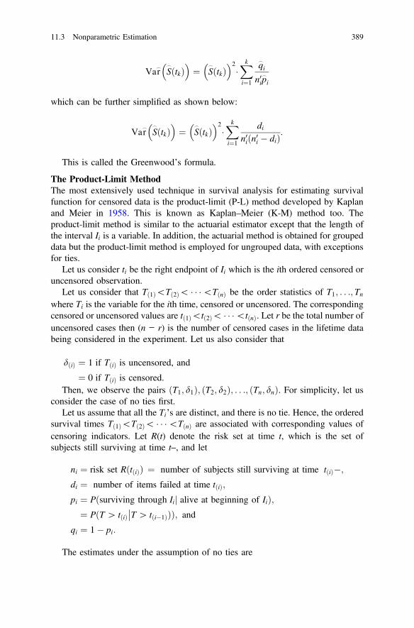
Var_ S_ðtkÞ
� �¼ S
_ðtkÞ� �2
�Xki¼1
q_i
n0ip_
i
which can be further simplified as shown below:
Var_ S_ðtkÞ
� �¼ S
_ðtkÞ� �2
�Xki¼1
din0iðn0i � diÞ:
This is called the Greenwood’s formula.
The Product-Limit MethodThe most extensively used technique in survival analysis for estimating survivalfunction for censored data is the product-limit (P-L) method developed by Kaplanand Meier in 1958. This is known as Kaplan–Meier (K-M) method too. Theproduct-limit method is similar to the actuarial estimator except that the length ofthe interval Ii is a variable. In addition, the actuarial method is obtained for groupeddata but the product-limit method is employed for ungrouped data, with exceptionsfor ties.
Let us consider ti be the right endpoint of Ii which is the ith ordered censored oruncensored observation.
Let us consider that Tð1Þ\Tð2Þ\ � � �\TðnÞ be the order statistics of T1; . . .; Tnwhere Ti is the variable for the ith time, censored or uncensored. The correspondingcensored or uncensored values are tð1Þ\tð2Þ\ � � �\tðnÞ. Let r be the total number ofuncensored cases then (n − r) is the number of censored cases in the lifetime databeing considered in the experiment. Let us also consider that
dðiÞ ¼ 1 if TðiÞ is uncensored, and
¼ 0 if TðiÞ is censored.Then, we observe the pairs ðT1; d1Þ; ðT2; d2Þ; . . .; ðTn; dnÞ. For simplicity, let us
consider the case of no ties first.Let us assume that all the Ti’s are distinct, and there is no tie. Hence, the ordered
survival times Tð1Þ\Tð2Þ\ � � �\TðnÞ are associated with corresponding values ofcensoring indicators. Let R(t) denote the risk set at time t, which is the set ofsubjects still surviving at time t–, and let
ni ¼ risk set RðtðiÞÞ ¼ number of subjects still surviving at time tðiÞ�;
di ¼ number of items failed at time tðiÞ;
pi ¼ Pðsurviving through Iij alive at beginning of IiÞ;¼ PðT [ tðiÞ T [ tði�1Þ
�� ÞÞ; and
qi ¼ 1� pi:
The estimates under the assumption of no ties are
11.3 Nonparametric Estimation 389

q_i ¼1ni;
p_i ¼ 1� q_i ¼ 1� 1ni
if dðiÞ ¼ 1 ðuncensoredÞ¼ 1 if dðiÞ ¼ 0 ðcensored.Þ
Then, the estimate for the survival function, S(t), under the assumption of no tiesis
SðtÞ ¼YtðiÞ � t
pi ¼YtðiÞ � t
1� 1ni
� dðiÞ
¼YtðiÞ � t
1� 1n� iþ 1
� dðiÞ¼
YtðiÞ � t
n� in� iþ 1
� dðiÞ:
If censored and uncensored observations are tied, let us consider that uncensoredobservations occurred just before the censored observations.
Now let us consider that there are r distinct survival times that can be arranged asorder statistics as follows:
t0ð1Þ\t0ð2Þ\ � � �\t0ðrÞ:
Then, let us define the following:
dðiÞ ¼ 1 if the observations at time t0ðiÞ are uncensored,
¼ 0; if censored,
ni ¼ number of subjects at risk in Rðt0ðiÞÞ;di ¼ number of failures at t0ðiÞ:
Then, the PL estimate for survival function can be obtained as follows for ties:
S_ðtÞ ¼
Yt0i � t
1� dini
� dðiÞ:
Variance of S_ðtÞ
We know that
S_ðtÞ ¼
Yt0ðiÞ � t
1� dini
� dðiÞ:
390 11 Survival Analysis

Taking loge, we obtain
lnS_ðtÞ ¼
XtðiÞ � t
dðiÞ ln 1� dini
� :
The estimate of the variance of survivor function can be shown as
Var_ðS_ðtÞÞ ¼ S_ðtÞh i2
:XtðiÞ � t
dðiÞq_
i
nip_
i
which can be further simplified as shown below:
Var_ðS_ðtÞÞ ¼ S_ðtÞh i2
:XtðiÞ � t
dðiÞdiniðni � diÞ :
This is the same Greenwood’s formula for estimating variance of survivalfunction displayed for the actuarial method.
Example 11.2 Suppose that a test has been carried out on a sample of 16 items, andthe observed lifetimes are (given in months)
5; 7; 9þ ; 14; 17; 19þ ; 20; 26; 30þ ; 40; 45; 46; 49þ ; 55; 61þ ; 69
where + indicates a censoring.The computation of P-L estimates is shown below for time of survival. The
censoring indicator 1 denotes uncensored and 0 denotes censored times(Table 11.7; Fig. 11.1).
Log-Rank TestWe know that
S_ðtÞ ¼
Yt0ðiÞ � t
1� dini
� dðiÞ:
If we want to compare survivor functions of two groups, such as treatment isgroup 1 and placebo is group 2, then we can use the log-rank test which isessentially a large sample chi-square test.
Let us consider that the combined set is ordered and the distinct times aredenoted by ti. Then
n1i = number of subjects in group 1 at risk at time ti,n2i = number of subjects in group 2 at risk at time ti,d1i = number of failures in group 1 at time ti,d2i = number of failures in group 2 at time ti,
11.3 Nonparametric Estimation 391
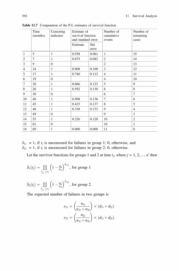
d1i = 1, if ti is uncensored for failures in group 1; 0, otherwise, andd2i = 1, if ti is uncensored for failures in group 2; 0, otherwise.
Let the survivor functions for groups 1 and 2 at time tj, where j = 1, 2,…, n0 then
S_
1ðtjÞ ¼Q
t0ðiÞ � tj
1� d1in1i
� �dð1iÞ, for group 1
S_
2ðtjÞ ¼Q
t0ðiÞ � tj
1� d2in2i
� �dð2iÞ, for group 2.
The expected number of failures in two groups is
e1i ¼ n1in1i þ n2i
� � ðd1i þ d2iÞ
e2i ¼ n2in1i þ n2i
� � ðd1i þ d2iÞ:
Table 11.7 Computation of the P-L estimates of survival function
Time(months)
Censoringindicator
Estimate ofsurvival functionand standard error
Number ofcumulativeevents
Number ofremainingcases
Estimate Std.error
1 5 1 0.938 0.061 1 15
2 7 1 0.875 0.083 2 14
3 9 0 2 13
4 14 1 0.808 0.100 3 12
5 17 1 0.740 0.112 4 11
6 19 0 4 10
7 20 1 0.666 0.123 5 9
8 26 1 0.592 0.130 6 8
9 30 0 6 7
10 40 1 0.508 0.136 7 6
11 45 1 0.423 0.137 8 5
12 46 1 0.338 0.133 9 4
13 49 0 9 3
14 55 1 0.226 0.128 10 2
15 61 0 10 1
16 69 1 0.000 0.000 11 0
392 11 Survival Analysis

Then, the (observed − expected) deaths in group 1 is
O1 � E1 ¼Xni¼1
d1i � e1ið Þ
and for group 2 is
O2 � E2 ¼Xni¼1
d2i � e2ið Þ:
Then, the log-rank statistic is defined as
v2 ¼ O2 � E2ð Þ2Var ðO2 � E2Þ
¼ O2 � E2ð Þ2Pni¼1
n1in2iðd1i þ d2iÞðn1i þ n2i�d1i�d2iÞðn1i þ n2iÞ2ðn1i þ n2i�1Þ
which is chi-square with 1 df under H0.
Fig. 11.1 Survival curve for the observed lifetimes of a sample of 16 subjects in a test
11.3 Nonparametric Estimation 393

11.4 Logistic Regression Model
In this section, the logistic regression model is introduced where the outcomevariables are dichotomous. Let Y = 1, if an event occurs during a defined studyperiod, Y = 0, otherwise. There are two primary reasons for choosing the logisticfunction in analyzing binary outcome data, from a mathematical point of view, it isan extremely flexible and easily used function, and it lends itself to biologicallymeaningful interpretation.
Let pðXÞ ¼ PðY ¼ 1 Xj Þ ¼ eb0 þ b1X
1þeb0 þ b1X
and 1� pðXÞ ¼ PðY ¼ 0 Xj Þ ¼ 1� eb0 þ b1X
1þeb0 þb1X¼ 1
1þeb0 þ b1X.
The log odds as a function of X is known as the logit transformation of pðXÞ thatcan be defined as follows:
gðXÞ ¼ lnpðXÞ
1� pðXÞ �
¼ lneb0 þb1X=ð1þ eb0 þb1XÞ
1=ð1þ eb0 þb1XÞ �
¼ ln eb0 þb1X� � ¼ b0 þ b1X:
This is a linear function and the logit function provides a linear logisticregression model.
Suppose we have a random sample of n pairs of observations (Xi; Yi), i = 1, 2,…,n. The outcome variable, Y, is a binary variable and X is the explanatory variable.The binary outcome variable represents presence or absence of the characteristic.The outcome variable can be represented by a Bernoulli distribution with parameterpðXÞ and the likelihood function is
LðbÞ ¼Yni¼1
LiðXiÞ ¼Yni¼1
pðXiÞ½ �Yi 1� pðXiÞ½ �1�Yi
¼Yni¼1
eb0 þb1Xi
1þ eb0 þ b1Xi
�Yi 11þ eb0 þb1Xi
�1�Yi
:
Taking log and differentiating with respect to the regression parameters, weobtain the estimating equations
Xni¼1
½Yi � pðXiÞ� ¼ 0; and
Xni¼1
Xi½Yi � pðXiÞ� ¼ 0:
Solving the above equations, we obtain the estimates for b0 and b1.
394 11 Survival Analysis
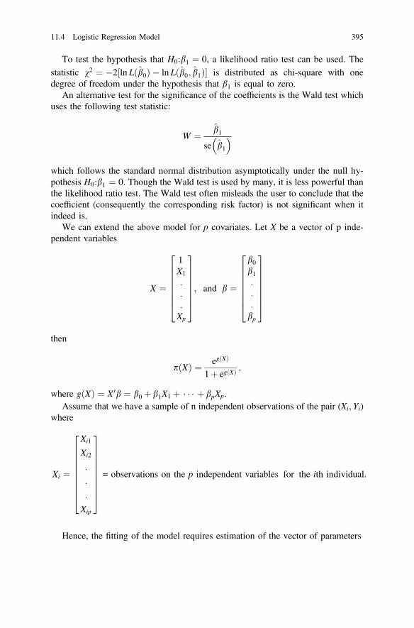
To test the hypothesis that H0:b1 ¼ 0, a likelihood ratio test can be used. Thestatistic v2 ¼ �2½ln Lðb0Þ � ln Lðb0; b1Þ� is distributed as chi-square with onedegree of freedom under the hypothesis that b1 is equal to zero.
An alternative test for the significance of the coefficients is the Wald test whichuses the following test statistic:
W ¼ b1
se b1� �
which follows the standard normal distribution asymptotically under the null hy-pothesis H0:b1 ¼ 0. Though the Wald test is used by many, it is less powerful thanthe likelihood ratio test. The Wald test often misleads the user to conclude that thecoefficient (consequently the corresponding risk factor) is not significant when itindeed is.
We can extend the above model for p covariates. Let X be a vector of p inde-pendent variables
X ¼
1X1
:::Xp
26666664
37777775; and b ¼
b0b1:::bp
26666664
37777775
then
pðXÞ ¼ egðXÞ
1þ egðXÞ;
where gðXÞ ¼ X 0b ¼ b0 þ b1X1 þ � � � þ bpXp.Assume that we have a sample of n independent observations of the pair (Xi; Yi)
where
Xi ¼
Xi1
Xi2
:
:
:
Xip
2666666664
3777777775= observations on the p independent variables for the ith individual.
Hence, the fitting of the model requires estimation of the vector of parameters
11.4 Logistic Regression Model 395

b ¼
b0b1:::bp
26666664
37777775:
The likelihood function is identical to that given for a single independent vari-able, with the only change being that pðXÞ is defined in terms of a multivariatelogit. There are (p + 1) likelihood equations which are obtained by differentiatingthe log-likelihood function with respect to the (p + 1) parameters b0; b1; . . .; bp.The estimating equations are
Xni¼1
Yi � pðXiÞ½ � ¼ 0
Xni¼1
Xij Yi � pðXiÞ½ � ¼ 0; j ¼ 1; 2; . . .; p:
From the second derivatives, we obtain
Iju ¼ �Xni¼1
XijXiupið1� piÞ; j; u ¼ 0; 1; . . .; p
where pi ¼ pðXiÞ. The information matrix is defined by the (p + 1) � (p + 1)matrix with (j, u)th element Iju ¼ ð�1Þ � Iju. Then, the variance–covariance matrixcan be defined as the inverse of the information matrix
RðbÞ ¼ I�1ðbÞ;
where jth diagonal element is the variance of the estimator of bj; j ¼ 0; 1; . . .; p:An approximate 100(1� a) percent confidence interval for bj can be obtained as
bj � z1�a=2
ffiffiffiffiffiffiffiI�1jj
q;
where z1�a=2 is the 100(1� a=2) percentile of the standard normal distribution.To test the hypothesis that some of the bj’s are zero, a likelihood ratio test can be
used. For testing the null hypothesis
H0:b1 ¼ b2 ¼ � � � ¼ bp ¼ 0
we can use the test statistic
396 11 Survival Analysis
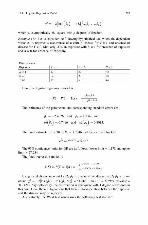
v2 ¼ �2 ln L b0� �
� ln L b0; b1; . . .; bp� �h i
which is asymptotically chi square with p degrees of freedom.
Example 11.3 Let us consider the following hypothetical data where the dependentvariable, Y, represents occurrence of a certain disease for Y = 1 and absence ofdisease for Y = 0. Similarly, X is an exposure with X = 1 for presence of exposureand X = 0 for absence of exposure.
Disease status
Exposure Y ¼ 1 Y ¼ 0 Total
X ¼ 1 17 30 47
X ¼ 0 2 20 22
Total 19 50 69
Here, the logistic regression model is
pðXÞ ¼ PðY ¼ 1 Xj Þ ¼ eb0 þ b1X
1þ eb0 þ b1X:
The estimates of the parameters and corresponding standard errors are
b0 ¼ �2:4026 and b1 ¼ 1:7346; and
se b0� �
¼ 0:7416 and se b1� �
¼ 0:8013:
The point estimate of lnOR is b1 ¼ 1:7346 and the estimate for OR
eb1 ¼ e1:7346 ¼ 5:667:
The 95% confidence limits for OR are as follows: lower limit = 1.178 and upperlimit = 27.254.
The fitted regression model is
pðXÞ ¼ PðY ¼ 1 Xj Þ ¼ e�2:3026þ 1:7346X
1þ e�2:3026þ 1:7346X :
Using the likelihood ratio test for H0:b1 ¼ 0 against the alternative H1:b1 6¼ 0, weobtain v2 ¼ �2½ln Lðb0Þ � ln Lðb0; b1Þ� = 81.216 − 74.917 = 6.2989 (p-value =0.0121). Asymptotically, the distribution is chi-square with 1 degree of freedom inthis case. Here, the null hypothesis that there is no association between the exposureand the disease may be rejected.
Alternatively, the Wald test which uses the following test statistic:
11.4 Logistic Regression Model 397
W ¼ b1
se b1� � ¼ 1:7346
0:8013¼ 2:1647 ðp-value ¼ 0:0340Þ
confirms the result based on the likelihood ratio test.
Example 11.4 This example uses a five percent random sample data from the wavefive of the Health and Retirement Study (HRS). Three hundred one subjectsincluded in this sample after removing the missing values for outcomes and riskfactors. The outcome is the depression status (Y = 0, 1), dichotomized (0 nodepression, 1 depression) based on a score using the scale proposed by the Centerfor Epidemiologic Studies of Depression (CESD). The explanatory variables con-sidered are age (in years) denoted by X1, gender (male = 1, female = 0) denoted byX2, marital status (MStatus) (married/partnered = 1, single/separated = 0) denotedby X3, BMI is denoted by X4, white race (1 yes, 0 no) denoted by X5 (other race isthe reference category), black race (1 yes, 0 no) denoted by X6 (other race is thereference category), drink (yes = 1, no = 0) denoted by X7, and number of con-ditions ever had (NCond) denoted by X8.
The overall fit of the model appears to be significant that means we may rejectthe null hypothesis
H0:b1 ¼ b2 ¼ � � � ¼ b8 ¼ 0:
The rejection of this null hypothesis implies that there is at least one logisticregression variable significantly associated with depression status. The likelihoodratio chi-square value is 61.5393 (p-value < 0.0001). The model fit statistics areshown in Table 11.8.
Among the selected variables, it appears that age, gender, and BMI do not showany statistically significant association with depression. However, the negativeassociation of depression status with marital status (p-value = 0.05), white race (p-value < 0.01) compared to other races, black race (p-value = 0.06) compared toother races, and drinking habit (p-value < 0.01) are observed. The number ofconditions shows a positive association with depression status (p-value < 0.001).
11.5 Models Based on Longitudinal Data
Survival analysis deals with events concerning survival status of subjects over timelongitudinally. The event status of the under consideration is observed repeatedlyover time. In contrast to longitudinal studies, cross-sectional studies provide singleoutcome for each individual at a point in time. The major advantages of a longi-tudinal study are that cohort and age effects can be studied in survival analysis usinglongitudinal data. In addition, the period effect can also be taken into account. Thelongitudinal data can be collected either prospectively, following subjects forward
398 11 Survival Analysis

in time, or retrospectively, by extracting multiple measurements on each personfrom historical records. The longitudinal data require special statistical methodsbecause the set of observations on one subject tends to be intercorrelated. Thiscorrelation needs to be taken into account to draw valid scientific inferences.Furthermore, the longitudinal data analysis involves the problem of censoring orloss to follow-up. This problem requires special attention as well for any validscientific conclusion.
Some important terms usually found in survival analysis are defined below.
LifetimeWe consider situations in which the time to the occurrence of some event is ofinterest for some population of individuals. The time to the occurrences of event istermed as lifetime. Mathematically, one can think of lifetime as merely meaningnonnegative valued variable. Although the term lifetime is used for general refer-ence, other terms such as survival time and failure time are also frequently used.
Table 11.8 Model fit statistics, estimates, and tests on the logistic regression model fordepression status among elderly people
A. Model fit statistics
Criterion Intercept only Intercept and covariates
AIC 440.671 395.132
SC 444.443 429.075
−2 Log L 438.671 377.132
B. Testing global null hypothesis beta = 0
Test Chi-square DF Pr > ChiSq
Likelihood ratio 61.5393 8 <0.0001
Score 53.4166 8 <0.0001
Wald 44.8382 8 <0.0001
C. Estimates and tests of parameters of the logistic regression model
Covariate Estimate Standarderror
Waldv2
p-value Odds ratio estimates
pointestimate
95% Waldconfidencelimits
Intercept 2.4501 2.8389 0.7449 0.3881
Age 0.00318 0.0401 0.0063 0.9369 1.003 0.927 1.085
Gender −0.0663 0.2631 0.0636 0.8010 0.936 0.559 1.567
MStatus −0.5893 0.3009 3.8348 0.0502 0.555 0.308 1.001
BMI 0.0158 0.0248 0.4058 0.5241 1.016 0.968 1.067
White −2.8780 1.0854 7.0304 0.0080 0.056 0.007 0.472
Black −2.1319 1.1340 3.5341 0.0601 0.119 0.013 1.095
Drink −0.7812 0.2561 9.3008 0.0023 0.458 0.277 0.756
NCond 0.4364 0.1109 15.475 <0.0001 1.547 1.245 1.923
11.5 Models Based on Longitudinal Data 399

Survival FunctionSurvival function is defined as the probability that an individual is surviving tilltime t and is defined by
SðtÞ ¼ P½T t�; t 0:
It is assumed that S(t) = 1 for t = 0.A survival function is the complementary to cumulative distribution function
since S(t) = 1 − F(t) for continuous random variables, where F(t) = P [T < t] is thecumulative distribution function. All survival functions must satisfy three condi-tions: S(0) = 1, lim
t!1 S(t) = 0, and S(t) is nonincreasing.
The conditional survival function, ST T aj ðtÞ, is the survival function of a ran-domly chosen subject given that the subject is surviving at time a. The conditionalsurvival function can be shown as
ST T aj ðtÞ ¼ PðT t and T aÞP ðT aÞ ¼ P ðT tÞ
P ðT aÞ ¼ S ðtÞS ðaÞ ; t a:
Probability Density FunctionThe probability density function of lifetime is defined by
f ðtÞ ¼ dFðtÞdt
¼ � dSðtÞdt
because S(t) = 1 − F(t). The probability of failure between times a and b is cal-culated by an integral
P ða� T � bÞ ¼Zb
a
f ðtÞdt:
Hazard FunctionThe hazard function is used most extensively for its ability to provide a measure ofthe amount of risk associated with a subject at time t and for making comparison ofthe risks and possible change in the risks over time. The hazard function is knownas the hazard rate, failure rate, force of mortality, force of decrement, intensityfunction, and age-specific death rate, and its reciprocal is known as Mill’s ratio ineconomics.
The hazard function can be derived by using the conditional probability. Let usconsider the probability of failure between t and t + D t
400 11 Survival Analysis

Pðt� T � tþDtÞ ¼ZtþDt
t
f ðsÞds ¼ SðtÞ � SðtþDtÞ:
Conditioning on the event that the subject is surviving at time t and then failsduring t and t +Dt
Pðt� T � tþDt T tj Þ ¼ Pðt� T � tþDtÞPðT tÞ ¼ SðtÞ � SðtþDtÞ
SðtÞ :
The average rate of failure is obtained if we divide by Dt
SðtÞ � SðtþDtÞSðtÞDt :
As Dt! 0, this becomes the instantaneous failure rate, which is the hazardfunction
hðtÞ ¼ limDt!0
SðtÞ � SðtþDtÞSðtÞDt
¼ �S0ðtÞSðtÞ ¼ f ðtÞ
SðtÞ ; t 0:
This shows that the hazard function is defined as the ratio of probability densityfunction and survival function at time t. All the hazard functions must satisfy thefollowing conditions:
Z/0
hðtÞdt ¼/ and hðtÞ 0 for all t 0:
The hazard function is important because it has a direct physical interpretation,and information about the nature of the function is useful in selecting an appropriatemodel for lifetime.
Cumulative Hazard FunctionThe cumulative hazard function, H(t), is defined as
HðtÞ ¼Z t
0
hðsÞds; t 0:
The cumulative hazard function satisfies three conditions: H(0) = 0,limt!1HðtÞ ¼ 1, and H(t) is nondecreasing.
11.5 Models Based on Longitudinal Data 401
Mean Time to Failure (MTTF)In survival analysis, the mean time to failure (MTTF) is often of interest. This isdefined by
EðTÞ ¼ l;
where
l ¼Z10
t f ðtÞ dt;
which can be obtained equivalently from the following equation:
l ¼Z10
SðtÞ dt:
Median LifeThe pth quantile (also known as the 100 pth percentile) of the distribution of T is thevalue tp so that F(tp) � p and S(tp) 1 − p. If T is a continuous random variablethen the pth quantile is found by solving the equation
SðtpÞ ¼ 1� p:
The median lifetime is the 50th percentile t0:5 so that Sðt0:5Þ ¼ 0:5:
Relationship between Survival Function and Hazard FunctionIt can be shown that the survival function and hazard function are associated in thefollowing form:
SðtÞ ¼ e�R t
0hðsÞds
;
and in terms of the cumulative hazard function, the survival function is
SðtÞ ¼ e�HðtÞ:
Using the definition of the hazard function, it is also evident that the probabilitydensity function of failure time is
f ðtÞ ¼ hðtÞ � SðtÞ
and using the relationships between SðtÞ and cumulative hazard or hazard functions,it can also be shown that
402 11 Survival Analysis
f ðtÞ ¼ hðtÞ � e�HðtÞ ¼ hðtÞ � e�R t
0hðsÞds
:
11.6 Proportional Hazards Model
The logistic regression is introduced in Sect. 11.4. Although the logistic regressionmodel is considered as a very important model for analyzing survival status, it doesnot address some of the important aspects necessary for understanding the survivalstatus adequately. In survival analysis, the lifetime or failure time is of core interest.In addition, the problems of censoring and truncation need to be considered insurvival analysis. It is noteworthy that time to failure data needs special attention,and modeling of survival data needs to consider censoring time along with failuretime of each subject in the sample. There is rarely any longitudinal data, particularlyin case of studies conducted for a longer duration for chronic diseases, where theproblem of censoring is not encountered. The dependence of failure times on risk orprognostic factors are of prime concern in analyzing survival data. We have toidentify the factors associated with the failure time not only by analyzing thesurvival status ignoring the time of event but by considering the time of event as theresponse variable. To address such problems, the proportional hazards modelprovides a regression model for analyzing failure time data that takes into accountpartial censoring. The proportional hazards model is expressed as a function of twocomponents: one component depends on time only, and the other componentdepends on risk or prognostic factors independent of time.
Let us represent the set of covariates by
Z ¼ ðZ1; Z2; . . .; ZpÞ
and the corresponding regression parameters are
b0 ¼ b1; b2; . . .; bp� �
:
The failure time is T. The survivor function is defined as
Sðt; zÞ ¼ PðT t Z ¼ zÞj :
The probability density function of survival or failure time is
f ðt; zÞ
and it can be obtained by differentiating the distribution function as follows:
11.5 Models Based on Longitudinal Data 403
@Fðt; zÞ@t
¼ f ðt; zÞ
where Fðt; zÞ ¼ 1� Sðt; zÞ which is the distribution function of the failure time, T.In the proportional hazards model, proposed by Cox (1972), the combined effect
of the Z variables is to scale the hazard function up or down. The hazard functionsatisfies
hðt; zÞ ¼ h0ðtÞ � gðzÞ;
where h0ðtÞ is the baseline hazard function. The regression model based on hazardfunction as proposed by Cox is
hðt; zÞ ¼ h0ðtÞezb¼ h0ðtÞeb1z1 þ ��� þ bpzp ;
where gðzÞ ¼ ezb:The ratio of hazard functions at time t for two subjects with covariate values
z1 and z2 is
hðt; z1Þhðt; z2Þ ¼
h0ðtÞgðz1Þh0ðtÞgðz2Þ ¼
gðz1Þgðz2Þ
which is independent of time, t. The hazards at different z values are in constantproportion over time. That is why the model is known as the proportional hazardsmodel. The function g zð Þ may take a variety of forms involving covariates z.
After taking natural log of the survival function, we obtain
ln Sðt; zÞ ¼ gðzÞ � ln S0ðtÞ:
It is known that
Sðt; zÞ ¼ e�R t
0hðs;zÞds
;
where hðt; zÞ ¼ h0ðtÞ � gðzÞ: Hence,
Sðt; zÞ ¼ ½S0ðtÞ�gðzÞ
that can be rewritten as
Sðt; zÞ ¼ ½S0ðtÞ�ezb
:
The baseline survival function is defined as
404 11 Survival Analysis

S0ðtÞ ¼ e�R t
0h ðsÞds
which is a function of time only, independent of covariates.Simple graphical analysis of data follows by plotting lnð� ln Sðt; zÞÞ for different
z values against some function of t, typically t or log t. If the proportional hazardsassumption holds, the plots should be similar curves shifted in the y-axis directionresulting in parallel lines.
The parameters are estimated by applying marginal or partial likelihoodapproaches. We cannot use the likelihood method directly for estimating theparameters of a proportional hazards model and the unknown arbitrary hazardfunctions cannot be estimated directly as well. As the estimates of the regressionparameters do not depend on the arbitrary or baseline hazard functions, the methodof estimation for proportional hazards regression produces estimates of regressionparameters without complicating the estimation procedure with estimation ofbaseline hazards at each time point.
If all the times are uncensored then the marginal likelihood is
LðbÞ ¼Yni¼1
ezðiÞbPl2RðtðiÞÞ e
ðzlbÞ
where RðtðiÞÞ is the risk set exposed to failure at ordered time tðiÞ, that is,
RðtðiÞÞ ¼ fðiÞ; ðiþ 1Þ; . . .; ðnÞg:
If there are censoring cases, then let us suppose that k distinct failure times aredenoted by the following order based on the rank of failure times as
1ð Þ; 2ð Þ; . . .:; kð Þ
where ordered failure times are
tð1Þ\tð2Þ\ � � �\tðkÞ
with corresponding covariates
zð1Þ; zð2Þ; . . .; zðkÞ
then the partial likelihood is
LðbÞ ¼Yki¼1
ezðiÞbPl2RðtðiÞÞ e
zlb;
11.6 Proportional Hazards Model 405

where RðtðiÞÞ ¼ f½ðjÞ; j1; . . .; jcj �; j ¼ i; . . .. . .; kg is the risk set for a failure at timetðiÞ and ci being number of censored cases during the interval ½tðiÞ; tðiþ 1ÞÞ. Similarly,the likelihood for ties can also be shown.
The value that maximizes the likelihood function can be obtained by a Newton–Raphson method. In the absence of ties, we can show that
b_ � Nðb; I�1ðb_ÞÞ:
There may be asymptotic bias in the estimation of both regression parametersand the variance–covariance of the estimators.
To test H0:b ¼ b0, the score statistic Uðb0Þ can be used where under H0
Uðb0Þ � Nð0; Iðb0ÞÞv2 � U0ðb0ÞI�1ðb0ÞUðb0Þ
can be shown approximately as v2 with p degrees of freedom.
Model Checking: Test for ProportionalityA simple test for proportionality assumption is introduced here. There are severalmethods including graphical methods but in this section, a simple procedure isintroduced so that anyone may use the method without any further complexity inthe application of the proportional hazards model. Let us consider the proportionalhazards model
hðt; zÞ ¼ h0ðtÞeb1z1 þ ��� þbpzp
where T is the survival time and Z1; . . .; Zp are the covariates. Now for testingwhether the proportionality assumption is violated by Zp, let us introduce a newvariable.
Now for testing whether the proportionality assumption is violated by Zp, let usintroduce a new variable
Zpþ 1 ¼ Zp � uðtÞ
where uðtÞ is a function of time such as (Kleinbaum and Klein 2012, p. 184)
uðtÞ ¼ t;
uðtÞ ¼ log t; and
uðtÞ ¼ 1 if t t0¼ 0 if t\t0:
Then, the extended proportional hazards model including the additional term as
406 11 Survival Analysis

hðt; zÞ ¼ h0ðtÞeb1z1 þ ��� þ bpzp þ bpþ 1zpþ 1
and after fitting the model let us test for the null hypothesis H0:bpþ 1 ¼ 0 versusH1:bpþ 1 6¼ 0.
The test statistic is
W ¼ bpþ 1
se bpþ 1
� � ;
where W is called a Wald test statistic and this can be shown as asymptotically N(0,1).
If the null hypothesis is rejected, then there is sufficient evidence that the pro-portionality assumption might be violated due to covariate Zp. In that case, eitherwe have to drop the covariate from the model and redo the estimation and test onceagain to arrive at a model that performs better. Another alternative is to perform astratified analysis in modeling the sample data. This procedure can be repeated byconsidering each variable as Zp and then continue the procedure until all thecovariates finally considered in the model are not causing violation of the pro-portionality assumption.
Now an extended method of assessing r (r < p) predictors at a time,Zpþ 1; . . .; Zpþ r, where these variables are defined by multiplying r selectedcovariates by u (t). The extended hazards model is
hðt; zÞ ¼ h0ðtÞeb1z1 þ ��� þ bpzp þ bpþ 1zpþ 1 þ ��� þbpþ rzpþ r :
We can employ the Wald test for all the interaction terms between covariates andtime (or function of time) as shown for a single variable previously.
If the null hypothesis is rejected, then it may be concluded that there is sufficientevidence in favor of violation of proportionality assumption by one or more of theselected covariates.
Example 11.5 Let us consider the data from a prospective study on maternalmorbidity in Bangladesh conducted by the Bangladesh Institute of Research forPromotion of Essential Reproductive Health and Technologies (BIRPERHT),during November 1992 to December 1993 (Akhter et al. 1996). The study wasconducted to identify the risk factors of complications at antenatal, delivery andpostnatal stages. In this example, excessive hemorrhage is considered as the out-come event. The outcome variable is defined as the time to excessive hemorrhageduring pregnancy. The women who did not experience any excessive hemorrhagecomplication during pregnancy are considered as censored and the censoring time isthe duration of pregnancy. The total number of pregnant women followed up was1020 out of which complete information was obtained on 993 pregnant women.The potential risk factors are age at marriage (<15 years = 0, as reference cate-gory, 15–19 years = 1, 20 + years = 2), desired pregnancy (No = 0, Yes = 1),
11.6 Proportional Hazards Model 407

education (no education as reference category, primary, secondary +), economicstatus (low = 0, high = 1).
The mean and median survival times, the corresponding standard errors, and95% confidence intervals are displayed. The mean survival time that is mean timefrom the beginning of the pregnancy to the time of first occurrence of excessivehemorrhage is 7.2 months with 95% confidence limits of 7.0 months to 7.4 months.This is estimated by using the Kaplan–Meier or Product-Limit method of survivalfunction. Out of 993 subjects, 12.5% had excessive hemorrhage complication. It isfound from the results displayed in Table 11.9 that age at marriage is negativelyand economic status is positively associated with excessive hemorrhage duringpregnancy (p-value < 0.05). We can say with caution that there might be a lowerrisk of excessive hemorrhage among pregnant women with higher level of edu-cation (p-value = 0.07). The test for proportionality shows that both age at marriageand economic status variables may be sources of violation of proportionalityassumption. Hence, a further examination of potential risk factors and outcomevariable is necessary. A careful investigation of the underlying relationshipsbetween the outcome variable and the potential risk factors as well as amongpotential risk factors may provide important insights in modeling the time toexcessive hemorrhage event during pregnancy (Table 11.10).
Table 11.9 Estimates of mean and median survival times and estimation and tests on theproportional hazards model on time to pregnancy complication of excessive hemorrhage
A. Data summary
Total N No. of events Censored
N Percent
993 124 869 87.5
B. Means and medians for survival time
Meana Median
Estimate Std. error 95% C.I. Estimate Std. error 95% C.I.
Lower Upper Lower Upper
7.212 0.092 7.031 7.393 7.566 0.246 7.083 8.048
C. Estimation of parameters of proportional hazards model and tests
B SE Wald df Sig. Exp(B)
Age at marriage −0.430 0.185 5.387 1 0.020 0.651
Desired pregnancy −0.062 0.191 0.103 1 0.748 0.940
Education −0.346 0.192 3.273 1 0.070 0.707
Economic status 0.541 0.211 6.547 1 0.011 1.718
408 11 Survival Analysis

11.7 Summary
In this chapter, the basic concepts and techniques of analyzing survival data areintroduced. Different study designs for collecting survival data are discussed, andthe corresponding procedures for estimating association between exposure anddisease such as relative risk or odds ratio are discussed. Also, the procedures forconstructing confidence intervals as well as for testing the hypothesis concerningany association between exposure and disease are highlighted for data fromprospective, case-control, and cross-sectional study designs. The nonparametricmethods of estimating survivor function are shown including the product-limitmethod. The variance of the estimator of survivor function is also obtained and thelog-rank test for comparing two survivor functions are also introduced in thischapter. One of the most widely used models in biostatistical data analysis is thelogistic regression model which is introduced in this chapter with examples. Theestimation and test procedures are discussed too. The basic concepts of longitudinaldata analysis are discussed and the proportional hazards model is introduced in thischapter with example. A simple method of model checking is also shown.
Exercises
11:1 Suppose the following data on Type 2 diabetes show the post prandial bloodglucose levels (<8.5 mmol/L = �E and 8.5 mmol/L = E) and status ofcertain complication (developed complication = D and did not developcomplication = �D) among the randomly selected subjects for groups E and �Ein a follow-up study.
Blood glucose level Developed complication ornot
D �D
E 20 80�E 7 93
Table 11.10 Test for proportionality assumption
B SE Wald df Sig. Exp(B)
Age at marriage −0.353 0.739 0.228 1 0.633 0.703
Desired pregnancy 1.710 0.660 6.715 1 0.010 5.528
Education 0.563 0.807 0.487 1 0.485 1.756
Economic status 1.917 0.787 5.931 1 0.015 6.803
Age at marriage * time −0.256 0.093 7.512 1 0.006 0.775
Desired pregnancy * time −0.128 0.116 1.217 1 0.270 0.880
Education * time 0.006 0.105 0.003 1 0.956 1.006
Economic status * time −0.222 0.120 3.410 1 0.065 0.801
Model chi-square = 55.825, df = 8 (p-value < 0.001)
11.7 Summary 409

(a) (i) Estimate the odds of developing complications in exposed andnonexposed groups.
(ii) Estimate the odds ratio of developing complications and interpret.(iii) Estimate the variance of the log odds ratio.(iv) Estimate the variance of the odds ratio.(v) Construct the 95% confidence intervals for the odds ratio.(vi) Test for the null hypothesis of H0: ln OR ¼ 0 against the alter-
native H1: ln OR 6¼ 0.(vii) What is your conclusion?
(b) (i) Estimate the risks of developing complications.(ii) Estimate the relative risk and interpret.(iii) Estimate the variance of the relative risk.(iv) Construct the 95% confidence interval for the relative risk.(v) Test for the null hypothesis of H0: ln RR ¼ 0 against the alter-
native H1: ln RR 6¼ 0.(vi) Comment on the association between exposure and developing
complication for Type 2 diabetes mellitus.
11:2 Consider the following table from a retrospective study to find the associa-tion between exposure (�E = not exposed and E = exposed) and occurrenceof disease (�D = case and D = control).
Disease status
Exposure status Case Control
E 25 30�E 475 1900
(i) Estimate the odds of developing complications in exposed and non-exposed groups.
(ii) Estimate the odds ratio of developing complications and interpret.(iii) Estimate the variance of the log odds ratio.(iv) Estimate the variance of the odds ratio.(v) Construct the 95% confidence intervals for the odds ratio.(vi) Test for the null hypothesis of H0: ln OR ¼ 0 against the alternative
H1: ln OR 6¼ 0.(vii) What is your conclusion?
410 11 Survival Analysis

11:3 In a cross-sectional study, the relationship between presence or absence of adisease and presence or absence of an exposure is obtained as displayed inthe following table:
Disease status
Exposure status Present (D) Absent (�D)
Present (E) 30 50
Absent (�E) 970 2450
(i) Estimate the odds ratio of presence of disease in the randomly selectedpopulation and interpret the value of the odds ratio.
(ii) Estimate the variance of the log odds ratio.(iii) Estimate the variance of the odds ratio.(iv) Construct the 95% confidence interval for the odds ratio.(v) Test for the null hypothesis of H0: ln OR ¼ 0 against the alternative
H1: ln OR 6¼ 0.(vi) What is your conclusion?
11:4 Consider the following data on time to event in months.
7; 10; 12; 15; 15þ ; 17þ ; 20; 22; 23þ ; 26; 35þ ; 39; 45; 54
(i) Estimate the survivor function using the product-limit method.(ii) Find the variance of the estimated survivor functions.(iii) Plot the product-limit estimates of the survivor function and interpret
the estimates of the survival function over time.
11:5 Consider the following hypothetical data show the remission times (in days)from high fever of patients selected in groups 1 and 2. The censored timesare denoted by a + sign.
Group 1:1; 2; 2; 3; 3þ ; 5; 5; 5þ ; 7; 10; 11; 12; 14; 15; 16þ ; 17; 19
Group 2:3; 4; 7; 7þ ; 9; 10; 11; 11þ ; 15; 15; 16; 17; 18; 20; 21þ ; 22; 24
(i) Estimate the survivor function for both groups 1 and 2, using theproduct-limit method.
(ii) Graphically plot the survivor functions, compare the survivor functions,and comment on the survival probabilities.
(iii) Estimate the variance of the estimated survivor functions for bothgroups 1 and 2.
11.7 Summary 411
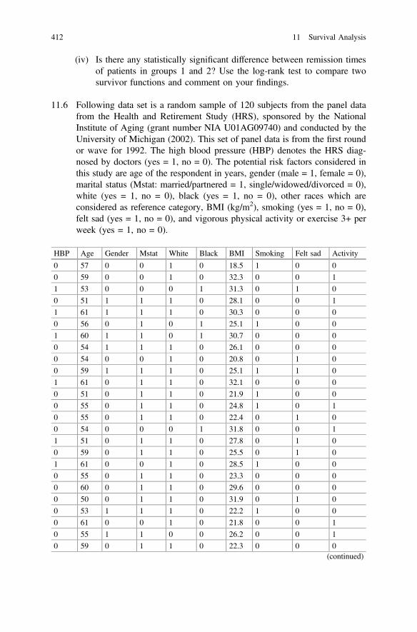
(iv) Is there any statistically significant difference between remission timesof patients in groups 1 and 2? Use the log-rank test to compare twosurvivor functions and comment on your findings.
11:6 Following data set is a random sample of 120 subjects from the panel datafrom the Health and Retirement Study (HRS), sponsored by the NationalInstitute of Aging (grant number NIA U01AG09740) and conducted by theUniversity of Michigan (2002). This set of panel data is from the first roundor wave for 1992. The high blood pressure (HBP) denotes the HRS diag-nosed by doctors (yes = 1, no = 0). The potential risk factors considered inthis study are age of the respondent in years, gender (male = 1, female = 0),marital status (Mstat: married/partnered = 1, single/widowed/divorced = 0),white (yes = 1, no = 0), black (yes = 1, no = 0), other races which areconsidered as reference category, BMI (kg/m2), smoking (yes = 1, no = 0),felt sad (yes = 1, no = 0), and vigorous physical activity or exercise 3+ perweek (yes = 1, no = 0).
HBP Age Gender Mstat White Black BMI Smoking Felt sad Activity
0 57 0 0 1 0 18.5 1 0 0
0 59 0 0 1 0 32.3 0 0 1
1 53 0 0 0 1 31.3 0 1 0
0 51 1 1 1 0 28.1 0 0 1
1 61 1 1 1 0 30.3 0 0 0
0 56 0 1 0 1 25.1 1 0 0
1 60 1 1 0 1 30.7 0 0 0
0 54 1 1 1 0 26.1 0 0 0
0 54 0 0 1 0 20.8 0 1 0
0 59 1 1 1 0 25.1 1 1 0
1 61 0 1 1 0 32.1 0 0 0
0 51 0 1 1 0 21.9 1 0 0
0 55 0 1 1 0 24.8 1 0 1
0 55 0 1 1 0 22.4 0 1 0
0 54 0 0 0 1 31.8 0 0 1
1 51 0 1 1 0 27.8 0 1 0
0 59 0 1 1 0 25.5 0 1 0
1 61 0 0 1 0 28.5 1 0 0
0 55 0 1 1 0 23.3 0 0 0
0 60 0 1 1 0 29.6 0 0 0
0 50 0 1 1 0 31.9 0 1 0
0 53 1 1 1 0 22.2 1 0 0
0 61 0 0 1 0 21.8 0 0 1
0 55 1 1 0 0 26.2 0 0 1
0 59 0 1 1 0 22.3 0 0 0(continued)
412 11 Survival Analysis

(continued)
HBP Age Gender Mstat White Black BMI Smoking Felt sad Activity
0 55 0 1 1 0 23.4 0 0 0
0 59 1 1 1 0 29.4 0 0 0
1 61 1 1 1 0 24.7 0 0 1
0 57 0 0 1 0 20.2 0 1 0
0 58 0 1 1 0 25.7 0 0 1
0 51 1 1 1 0 25.8 0 1 0
0 61 1 1 1 0 27.3 0 0 0
1 52 1 1 1 0 28.4 0 0 1
0 51 1 1 1 0 27.6 1 1 0
0 57 0 1 1 0 28.2 0 0 0
0 51 1 0 1 0 23.7 0 0 1
1 60 1 1 1 0 38 0 0 0
1 53 0 1 0 1 32.3 0 0 0
0 56 0 1 1 0 27.1 1 1 0
0 56 0 1 1 0 27.9 0 1 1
0 58 0 1 1 0 25.8 0 1 0
0 52 1 1 1 0 21.6 1 0 0
0 56 0 0 1 0 24.1 0 1 0
0 55 1 1 1 0 30.4 1 0 0
0 60 0 1 1 0 32 0 1 0
1 59 0 1 1 0 25.5 0 1 0
1 56 1 1 1 0 35.3 0 0 0
1 51 0 0 1 0 23 1 1 1
1 51 0 0 1 0 29.3 0 1 0
1 60 0 1 0 1 24.8 1 1 1
0 52 1 1 1 0 23.6 0 1 0
0 56 0 1 1 0 21.3 0 1 0
0 55 0 1 1 0 23.8 0 0 1
0 55 1 1 1 0 31.7 0 0 1
0 56 0 1 1 0 23.5 0 0 0
0 52 1 1 1 0 29 0 0 0
0 61 1 1 1 0 23.7 0 0 1
1 60 0 1 1 0 34.3 0 1 1
1 54 0 1 1 0 31.3 0 0 0
1 54 1 1 0 0 27 0 1 0
0 61 0 1 1 0 20.3 0 0 0
0 52 1 0 1 0 24.4 0 1 1
0 59 1 1 1 0 26.9 0 0 0
0 53 1 1 1 0 24 1 0 0
1 52 0 1 1 0 35.4 0 0 0(continued)
11.7 Summary 413

(continued)
HBP Age Gender Mstat White Black BMI Smoking Felt sad Activity
0 58 0 1 1 0 32.9 0 1 1
1 55 0 1 1 0 25.6 1 0 1
0 60 1 1 1 0 25.7 0 1 1
0 58 1 1 1 0 32.8 0 0 0
1 59 1 1 1 0 29.6 0 0 0
0 55 1 1 1 0 29.4 0 0 0
0 55 0 1 1 0 25.2 0 1 0
1 54 0 1 1 0 23.4 0 1 0
1 56 1 1 1 0 28.5 0 0 0
1 51 0 0 1 0 24.5 1 0 0
1 52 0 1 1 0 31.9 1 1 0
0 55 1 1 1 0 22.7 0 0 0
0 57 0 0 1 0 24.6 0 0 1
0 58 1 1 0 1 20.8 1 1 0
1 54 0 0 0 0 35.4 0 0 0
1 57 0 0 0 1 26.2 0 0 0
1 61 0 1 0 1 27.3 0 0 1
1 56 1 1 0 1 28.1 1 1 0
1 54 0 1 0 1 32.1 0 0 1
1 53 0 0 1 0 31.3 0 1 0
0 56 1 1 1 0 27.3 0 1 0
0 52 0 1 1 0 27.8 0 1 0
1 55 0 0 1 0 20.5 0 0 0
0 53 1 1 1 0 32.1 0 0 0
0 61 0 0 1 0 20.6 0 1 0
1 60 1 0 1 0 28.8 0 0 0
0 57 1 1 1 0 23.1 0 0 0
0 57 1 0 0 1 27.3 1 0 0
0 54 1 1 0 1 27.3 0 0 0
0 51 1 1 1 0 24 0 0 0
0 56 0 1 1 0 24.2 0 0 0
0 56 0 1 1 0 23.5 0 1 0
0 53 0 1 1 0 19.9 0 1 0
0 58 1 1 1 0 27.3 0 1 0
0 54 1 1 1 0 25 1 0 0
0 51 0 1 1 0 22 0 1 0
0 53 1 1 1 0 45.3 0 1 0
1 52 0 1 1 0 33.7 0 1 1
0 59 1 1 1 0 27.7 0 0 0
1 57 0 1 1 0 26.6 0 0 0(continued)
414 11 Survival Analysis

(continued)
HBP Age Gender Mstat White Black BMI Smoking Felt sad Activity
1 59 1 1 1 0 25.7 0 1 0
1 55 0 1 1 0 35.4 0 1 0
1 55 1 1 1 0 25.1 0 0 0
0 58 1 0 0 1 27.9 1 0 0
1 56 0 1 0 1 36.6 0 1 0
0 56 1 1 1 0 21.6 1 0 0
0 55 0 1 1 0 22.5 0 0 0
0 55 0 1 1 0 18.3 0 0 1
1 58 1 1 1 0 38.4 0 0 0
1 55 1 1 0 1 31 1 0 1
0 61 1 1 1 0 21.6 1 0 1
0 56 1 1 1 0 28 1 0 1
0 57 0 1 1 0 19.9 1 1 0
0 59 1 1 1 0 27.3 0 1 0
0 55 1 1 1 0 28.5 0 0 0
HRS (2017). Health and Retirement Study, University of Michigan, Ann Arbor, 1992–2014. Theauthors gratefully acknowledge the support of HRS (Health and Retirement Study) which issponsored by the National Institute of Aging (grant number NIA U01AG09740) and conducted bythe University of Michigan for the data
(i) Conduct an exploratory analysis to find the association between highblood pressure (HBP) and selected potential risk factors.
(ii) Fit a logistic regression model for high blood pressure to identify thenature of relationship between potential risk factors and HBP.
(iii) Comment on the goodness of fit of the model.(iv) Test for the significance of the parameters and comment on the
association between high blood pressure and potential risk factors.(v) Estimate the odds ratios from the model and interpret.(vi) Find the 95% confidence interval for the population odds ratios.
11:7 Following data set is a random sample of 155 subjects from the panel datafrom the Health and Retirement Study (HRS), sponsored by the NationalInstitute of Aging (grant number NIA U01AG09740) and conducted by theUniversity of Michigan (2002). We have used the panel data from the secondto eleventh round or wave. The variable “Time” is time to event since theentry to the study. The event of interest is the first time occurrence of heartproblem since the last interview. The event heart (yes = 1, no = 0) denoteswhether heart disease was diagnosed or not, yes indicating event and no forcensored cases. Covariates are age (in years), gender (male = 1, female = 0),Hispanic (yes = 1, no = 0), drink (yes = 1, no = 0), smoking (yes = 1, no = 0),body mass index (BMI), doctor diagnosed high blood pressure (Hibps)(yes = 1, no = 0), and the number of previous conditions.
11.7 Summary 415

Time Heart Age Gender Hispanic Drink BMI Number of prev.condition
Hibps Smoke
17.9 0 61 0 1 1 25.2 0 0 0
23.0 0 70 1 0 1 31.3 4 0 0
16.9 0 72 1 0 1 29.1 4 0 0
24.7 1 53 0 0 0 26.6 5 0 1
21.9 1 67 0 0 0 21.0 3 0 0
23.0 1 74 1 0 1 27.1 2 0 0
25.0 0 77 0 0 0 32.4 3 1 0
23.0 1 60 0 0 0 28.1 2 0 1
18.0 0 72 1 0 0 29.1 3 0 0
29.0 0 71 0 0 0 31.9 3 0 0
19.0 0 81 0 0 1 27.4 4 0 0
22.0 0 65 0 0 0 25.6 2 1 0
25.9 1 67 0 0 0 30.9 6 0 0
20.7 1 56 1 0 0 24.5 2 0 1
17.9 0 74 0 0 0 28.2 3 0 0
21.9 0 65 0 0 0 23.6 5 0 0
20.0 0 79 0 0 0 31.4 3 0 0
24.5 0 55 0 0 1 24.5 1 0 0
13.0 0 72 1 1 1 23.6 2 0 1
21.7 1 62 1 0 0 25.1 3 0 0
26.0 0 72 1 0 0 28.9 3 0 0
24.2 0 55 1 0 0 27.1 2 0 0
25.9 0 69 1 0 1 27.5 2 0 0
25.0 0 75 1 0 0 27.1 2 0 0
22.0 0 79 0 0 1 22.3 1 0 0
19.0 0 75 1 0 0 29.3 1 0 0
23.0 0 76 0 0 1 25.2 3 0 0
24.9 0 55 0 0 0 32.7 2 0 0
23.1 0 57 0 0 0 20.4 3 0 0
21.0 1 65 1 0 0 29.8 2 0 0
21.0 0 69 1 0 0 29.7 3 1 1
22.0 1 64 0 0 0 36.8 4 0 0
21.0 0 73 0 0 1 25.1 4 0 0
25.9 1 63 0 0 1 30.2 6 0
21.0 0 68 0 0 1 22.1 4 0 1
26.0 0 74 0 1 1 23.7 3 0 0
26.0 0 75 0 0 0 35.7 2 0 0
24.9 0 73 0 0 0 27.5 4 0 0
19.0 0 71 0 0 1 19.4 1 0 0
20.5 0 52 0 0 1 29.5 0 0 0
28.0 0 77 1 0 0 31.0 4 0 0(continued)
416 11 Survival Analysis

(continued)
Time Heart Age Gender Hispanic Drink BMI Number of prev.condition
Hibps Smoke
24.0 0 62 1 0 1 23.7 1 0 0
26.0 0 63 1 0 1 31.4 2 0 0
25.0 0 76 1 0 0 32.1 2 0 0
26.0 0 60 0 0 1 22.5 0 0 0
17.9 0 75 0 0 1 30.0 3 0 0
22.2 1 60 0 0 0 32.9 4 0 0
22.9 0 66 1 0 1 44.8 1 0 0
19.0 1 77 1 0 1 21.8 4 0 0
25.0 1 69 1 0 1 35.5 3 0 0
21.9 1 70 1 0 1 29.3 3 0 0
22.0 1 67 0 0 0 23.4 5 0 0
29.9 0 67 1 0 0 26.3 0 0 1
28.0 0 69 0 0 1 27.4 4 0 0
19.0 0 79 0 0 1 33.9 6 0 0
19.0 0 80 1 0 1 30.8 4 0 0
17.0 0 72 0 0 0 24.4 1 0 0
23.0 0 78 1 0 0 28.4 5 0 0
25.0 0 78 0 0 1 27.6 3 0 0
23.0 0 66 0 0 1 23.6 4 0 1
21.0 0 62 1 0 0 19.2 3 0 1
20.6 0 58 1 0 1 24.5 2 0 0
32.0 1 74 1 0 1 22.0 3 0 0
19.9 0 60 0 1 0 30.3 0 0 0
21.9 0 67 1 0 0 27.0 7 0 0
23.0 0 64 0 1 0 15.6 4 0 1
25.4 0 63 0 0 1 25.1 3 0 0
19.0 0 80 0 0 0 29.3 3 1 0
32.0 0 59 0 0 0 17.9 1 0 0
29.0 0 68 1 0 1 32.1 2 0 0
26.0 1 63 1 0 1 28.0 2 0 1
24.0 0 61 0 0 1 27.3 2 0 0
23.9 0 66 0 0 1 28.3 2 0 0
15.9 0 75 1 0 1 25.1 3 0 0
17.0 0 79 1 0 0 22.2 1 0 0
18.0 0 75 0 0 0 29.1 2 0 0
26.0 1 77 0 0 0 25.2 4 0 0
20.0 0 68 0 0 0 22.7 0 0 0
22.0 0 75 0 0 0 22.6 2 0 0
20.0 0 78 0 0 0 22.5 3 0 1
25.9 0 69 1 0 1 25.6 0 0 0(continued)
11.7 Summary 417
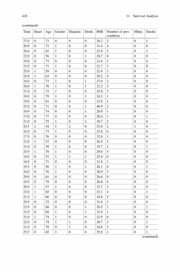
(continued)
Time Heart Age Gender Hispanic Drink BMI Number of prev.condition
Hibps Smoke
27.0 0 73 0 0 0 20.2 2 0 1
20.9 0 73 1 0 0 31.4 4 0 0
26.6 0 61 1 0 0 23.8 3 0 1
23.9 0 56 1 0 1 28.7 0 0 0
19.0 0 73 0 0 0 21.6 3 0 0
23.9 0 71 1 0 0 21.7 3 0 0
25.0 1 59 0 0 0 22.4 3 0 0
25.8 1 63 0 0 0 39.2 4 0 0
24.0 0 73 1 0 1 27.0 2 0 0
28.0 1 70 1 0 1 22.2 2 0 0
21.0 0 73 1 0 0 25.8 3 0 0
19.0 0 79 1 0 1 24.3 1 0 0
19.0 0 81 0 0 0 32.9 1 0 0
23.0 0 71 0 0 1 40.9 2 0 0
19.9 0 74 0 0 1 28.9 1 0 0
17.0 0 77 0 0 0 20.4 1 0 1
21.0 0 75 1 0 1 30.7 2 0 0
24.5 1 54 1 1 0 25.8 2 1 0
24.9 0 73 1 0 0 25.8 0 0 0
17.9 0 76 0 0 0 32.0 1 0 0
23.0 1 57 0 0 0 26.5 2 0 0
31.0 0 59 1 0 0 19.7 2 0 1
25.9 1 78 1 0 0 29.0 5 0 0
19.9 0 57 1 1 1 25.4 0 0 0
16.9 0 71 0 0 0 21.8 1 0 0
19.5 0 56 1 0 1 28.1 0 0 1
24.0 0 76 1 0 0 26.9 3 0 0
29.0 0 61 0 0 0 26.6 0 0 0
19.9 0 79 0 0 0 26.8 4 0 0
20.9 1 57 1 0 0 33.7 3 0 0
23.0 1 65 0 0 0 23.1 4 0 1
21.9 1 66 0 0 0 34.8 5 0 0
29.9 0 72 0 0 0 31.6 3 0 0
23.9 0 68 0 0 1 20.5 1 0 1
31.9 0 69 1 0 1 31.9 1 0 0
31.0 1 74 1 0 0 22.9 6 0 0
22.0 0 74 1 1 0 28.7 3 0 1
21.0 0 78 0 1 0 24.8 3 0 0
25.5 0 65 1 0 0 25.8 1 0 1(continued)
418 11 Survival Analysis

(continued)
Time Heart Age Gender Hispanic Drink BMI Number of prev.condition
Hibps Smoke
26.0 0 65 0 0 1 26.1 3 0 1
23.1 0 59 1 0 1 25.1 1 0 1
26.0 0 71 1 0 0 28.7 4 0 0
23.0 1 75 0 0 0 28.3 1 0 0
23.4 0 62 0 0 1 24.2 3 0
17.9 0 71 0 0 0 24.9 3 0 0
23.0 0 58 0 0 0 27.5 1 0 1
27.0 0 73 0 0 0 37.4 4 0 0
18.0 0 72 1 0 1 28.1 3 0 0
22.0 0 72 0 0 1 25.4 3 0 1
23.3 0 65 1 0 0 23.5 3 0 0
19.9 0 73 0 0 1 19.0 5 0 1
27.0 0 80 1 0 1 25.8 4 0 0
17.0 0 76 1 0 0 30.4 3 0 0
19.0 1 65 0 1 0 33.8 4 1 0
21.0 1 57 1 0 0 25.5 2 0 1
21.2 0 62 0 0 0 23.0 3 0 0
14.9 0 71 0 0 1 24.2 1 0 0
17.0 0 71 1 0 1 23.0 1 0 0
25.0 0 81 1 0 1 21.6 2 0 1
20.0 0 78 0 0 0 25.1 3 0 0
30.0 0 59 0 0 0 21.3 1 0 0
21.0 0 77 1 0 0 25.8 2 0 0
27.0 0 71 1 0 0 27.4 1 0 0
21.0 0 65 0 0 1 26.5 1 0 0
22.9 0 60 1 0 0 29.0 2 0 0
29.9 0 68 0 0 0 23.5 1 0 0
25.0 0 68 1 0 0 30.0 3 0 0
27.0 1 58 1 0 1 33.1 3 1 1
21.0 0 66 0 0 0 32.6 3 0 0
17.0 0 70 1 0 0 23.3 1 0 0
26.0 1 69 0 0 1 33.2 5 0 0
17.9 0 70 1 0 0 33.9 2 0 0
23.1 0 55 0 0 0 23.0 0 0 1
17.5 0 72 0 0 1 39.8 2 0 0
HRS ((Health And Retirement Study) 2017). Health and Retirement Study, University ofMichigan, Ann Arbor, 1992–2014. The authors gratefully acknowledge the support of HRS(Health and Retirement Study) which is sponsored by the National Institute of Aging (grantnumber NIA U01AG09740) and conducted by the University of Michigan for the data
11.7 Summary 419

(i) Estimate the relative risk and odds ratio of the occurrence of heartdisease for each of the potential risk factors considered in this example.Comment on your results.
(ii) Test for the association between exposure and occurrence of heartdisease from the data.
(iii) Propose a proportional hazards model for analyzing the time tooccurrence of heart disease.
(iv) Fit a proportional hazards model and comment on the overall fit as wellas significance of each variable included in the model.
(v) Check for the proportionality assumption for each covariate selected inthe model and summarize your comments.
(vi) Summarize your findings from (i) to (v) and comment on the suitabilityof your model for analyzing the heart disease data.
References
Akhter, H. H., Chowdhury, M. E. E. K., & Sen, A. (1996). A cross-sectional study on maternalmorbidity in Bangladesh. Dhaka, Bangladesh: BIRPERHT.
Cox, D. R. (1972). Regression models and life tables (with discussion). Journal of the RoyalStatistical Society B, 34, 187–220.
HRS (Health And Retirement Study) (2017). Public use dataset. Produced and distributed by theUniversity of Michigan with funding from the National Institute on Aging (grant numberNIAU01AG09740). Ann Arbor, MI.
Kaplan, E. L., & Meier, P. (1958). Nonparametric estimation from incomplete observations.Journal of the American Statistical Association, 53, 457–481.
Kleinbaum, D. G., & Klein, M. (2012). Survival analysis a self-learning text (3rd ed.). New York:Springer Publishers.
Mausner, J. S., & Kramer, S. (1985). Mausner & Bahn Epidemiology- An Introductory Text (2nded.). Philadelphia: W.B. Saunders Company.
420 11 Survival Analysis

Appendix
Table A.1: Binomial Cumulative Distribution Function
The tabulated value is P X� � xð Þ, where X has the binomial distribution withindex n and parameter p, for a selection of values of n and p.
© Springer Nature Singapore Pte Ltd. 2018M. A. Islam and A. Al-Shiha, Foundations of Biostatistics,https://doi.org/10.1007/978-981-10-8627-4
421
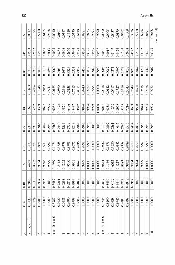
p=
0.05
0.10
0.15
0.20
0.25
0.30
0.35
0.40
0.45
0.50
n=5,
x=0
0.77
380.59
050.44
370.32
770.23
730.16
810.11
600.07
780.05
030.03
12
10.97
740.91
850.83
520.73
730.63
280.52
820.42
840.33
700.25
620.18
75
20.99
880.99
140.97
340.94
210.89
650.83
690.76
480.68
260.59
310.50
00
31.00
000.99
950.99
780.99
330.98
440.96
920.94
600.91
300.86
880.81
25
41.00
001.00
000.99
990.99
970.99
900.99
760.99
470.98
980.98
150.96
88
n=10
,x=0
0.59
870.34
870.19
690.10
740.05
630.02
820.01
350.00
600.00
250.00
10
10.91
390.73
610.54
430.37
580.24
400.14
930.08
600.04
640.02
330.01
07
20.98
850.92
980.82
020.67
780.52
560.38
280.26
160.16
730.09
960.05
47
30.99
900.98
720.95
000.87
910.77
590.64
960.51
380.38
230.26
600.17
19
40.99
990.99
840.99
010.96
720.92
190.84
970.75
150.63
310.50
440.37
70
51.00
000.99
990.99
860.99
360.98
030.95
270.90
510.83
380.73
840.62
30
61.00
001.00
000.99
990.99
910.99
650.98
940.97
400.94
520.89
800.82
81
71.00
001.00
001.00
000.99
990.99
960.99
840.99
520.98
770.97
260.94
53
81.00
001.00
001.00
001.00
001.00
000.99
990.99
950.99
830.99
550.98
93
91.00
001.00
001.00
001.00
001.00
001.00
001.00
000.99
990.99
970.99
90
n=15
,x=0
0.46
330.20
590.08
740.03
520.01
340.00
470.00
160.00
050.00
010.00
00
10.82
900.54
900.31
860.16
710.08
020.03
530.01
420.00
520.00
170.00
05
20.96
380.81
590.60
420.39
800.23
610.12
680.06
170.02
710.01
070.00
37
30.99
450.94
440.82
270.64
820.46
130.29
690.17
270.09
050.04
240.01
76
40.99
940.98
730.93
830.83
580.68
650.51
550.35
190.21
730.12
040.05
92
50.99
990.99
780.98
320.93
890.85
160.72
160.56
430.40
320.26
080.15
09
61.00
000.99
970.99
640.98
190.94
340.86
890.75
480.60
980.45
220.30
36
71.00
001.00
000.99
940.99
580.98
270.95
000.88
680.78
690.65
350.50
00
81.00
001.00
000.99
990.99
920.99
580.98
480.95
780.90
500.81
820.69
64
91.00
001.00
001.00
000.99
990.99
920.99
630.98
760.96
620.92
310.84
91
101.00
001.00
001.00
001.00
000.99
990.99
930.99
720.99
070.97
450.94
08(con
tinued)
422 Appendix

(con
tinued)
p=
0.05
0.10
0.15
0.20
0.25
0.30
0.35
0.40
0.45
0.50
111.00
001.00
001.00
001.00
001.00
000.99
990.99
950.99
810.99
370.98
24
121.00
001.00
001.00
001.00
001.00
001.00
000.99
990.99
970.99
890.99
63
131.00
001.00
001.00
001.00
001.00
001.00
001.00
001.00
000.99
990.99
95
141.00
001.00
001.00
001.00
001.00
001.00
001.00
001.00
001.00
001.00
00
n=20
,x=0
0.35
850.12
160.03
880.01
150.00
320.00
080.00
020.00
000.00
000.00
00
10.73
580.39
170.17
560.06
920.02
430.00
760.00
210.00
050.00
010.00
00
20.92
450.67
690.40
490.20
610.09
130.03
550.01
210.00
360.00
090.00
02
30.98
410.86
700.64
770.41
140.22
520.10
710.04
440.01
600.00
490.00
13
40.99
740.95
680.82
980.62
960.41
480.23
750.11
820.05
100.01
890.00
59
50.99
970.98
870.93
270.80
420.61
720.41
640.24
540.12
560.05
530.02
07
61.00
000.99
760.97
810.91
330.78
580.60
800.41
660.25
000.12
990.05
77
71.00
000.99
960.99
410.96
790.89
820.77
230.60
100.41
590.25
200.13
16
81.00
000.99
990.99
870.99
000.95
910.88
670.76
240.59
560.41
430.25
17
91.00
001.00
000.99
980.99
740.98
610.95
200.87
820.75
530.59
140.41
19
101.00
001.00
001.00
000.99
940.99
610.98
290.94
680.87
250.75
070.58
81
111.00
001.00
001.00
000.99
990.99
910.99
490.98
040.94
350.86
920.74
83
121.00
001.00
001.00
001.00
000.99
980.99
870.99
400.97
900.94
200.86
84
131.00
001.00
001.00
001.00
001.00
000.99
970.99
850.99
350.97
860.94
23
141.00
001.00
001.00
001.00
001.00
001.00
000.99
970.99
840.99
360.97
93
151.00
001.00
001.00
001.00
001.00
001.00
001.00
000.99
970.99
850.99
41
161.00
001.00
001.00
001.00
001.00
001.00
001.00
001.00
000.99
970.99
87
171.00
001.00
001.00
001.00
001.00
001.00
001.00
001.00
001.00
000.99
98
181.00
001.00
001.00
001.00
001.00
001.00
001.00
001.00
001.00
001.00
00
Ackno
wledg
edthatthecopy
righ
tbelon
gsto
theRoy
alStatisticalSo
cietyandreprod
uced
from
theRoy
alStatisticalSo
cietyTables,Roy
alStatisticalSo
ciety,
2004
with
perm
ission
from
theRoy
alStatistical
Society.
Appendix 423

Table A.2: Poisson Cumulative Distribution Function
The tabulated value is P X� � xð Þ, where X has the Poisson distribution withparameter l for a selected values of l
424 Appendix

0.5
1.0
1.5
2.0
2.5
3.0
3.5
4.0
4.5
5.0
x0
0.60
650.36
790.22
310.13
530.08
210.04
980.03
020.01
830.01
110.00
67
10.90
980.73
580.55
780.40
600.28
730.19
910.13
590.09
160.06
110.04
04
20.98
560.91
970.80
880.67
670.54
380.42
320.32
080.23
810.17
360.12
47
30.99
820.98
100.93
440.85
710.75
760.64
720.53
660.43
350.34
230.26
50
40.99
980.99
630.98
140.94
730.89
120.81
530.72
540.62
880.53
210.44
05
51.00
000.99
940.99
550.98
340.95
800.91
610.85
760.78
510.70
290.61
60
61.00
000.99
990.99
910.99
550.98
580.96
650.93
470.88
930.83
110.76
22
71.00
001.00
000.99
980.99
890.99
580.98
810.97
330.94
890.91
340.86
66
81.00
001.00
001.00
000.99
980.99
890.99
620.99
010.97
860.95
970.93
19
91.00
001.00
001.00
001.00
000.99
970.99
890.99
670.99
190.98
290.96
82
101.00
001.00
001.00
001.00
000.99
990.99
970.99
900.99
720.99
330.98
63
111.00
001.00
001.00
001.00
001.00
000.99
990.99
970.99
910.99
760.99
45
121.00
001.00
001.00
001.00
001.00
001.00
000.99
990.99
970.99
920.99
80
131.00
001.00
001.00
001.00
001.00
001.00
001.00
000.99
990.99
970.99
93
141.00
001.00
001.00
001.00
001.00
001.00
001.00
001.00
000.99
990.99
98
151.00
001.00
001.00
001.00
001.00
001.00
001.00
001.00
001.00
000.99
99
161.00
001.00
001.00
001.00
001.00
001.00
001.00
001.00
001.00
001.00
00
5.5
6.0
6.5
7.0
7.5
8.0
8.5
9.0
9.5
10.0
x0
0.00
410.00
250.00
150.00
090.00
060.00
030.00
020.00
010.00
010.00
00
10.02
660.01
740.01
130.00
730.00
470.00
300.00
190.00
120.00
080.00
05
20.08
840.06
200.04
300.02
960.02
030.01
380.00
930.00
620.00
420.00
28
30.20
170.15
120.11
180.08
180.05
910.04
240.03
010.02
120.01
490.01
03
40.35
750.28
510.22
370.17
300.13
210.09
960.07
440.05
500.04
030.02
93
50.52
890.44
570.36
900.30
070.24
140.19
120.14
960.11
570.08
850.06
71
60.68
600.60
630.52
650.44
970.37
820.31
340.25
620.20
680.16
490.13
01(con
tinued)
Appendix 425

(con
tinued)
0.5
1.0
1.5
2.0
2.5
3.0
3.5
4.0
4.5
5.0
70.80
950.74
400.67
280.59
870.52
460.45
300.38
560.32
390.26
870.22
02
80.89
440.84
720.79
160.72
910.66
200.59
250.52
310.45
570.39
180.33
28
90.94
620.91
610.87
740.83
050.77
640.71
660.65
300.58
740.52
180.45
79
100.97
470.95
740.93
320.90
150.86
220.81
590.76
340.70
600.64
530.58
30
110.98
900.97
990.96
610.94
670.92
080.88
810.84
870.80
300.75
200.69
68
120.99
550.99
120.98
400.97
300.95
730.93
620.90
910.87
580.83
640.79
16
130.99
830.99
640.99
290.98
720.97
840.96
580.94
860.92
610.89
810.86
45
140.99
940.99
860.99
700.99
430.98
970.98
270.97
260.95
850.94
000.91
65
150.99
980.99
950.99
880.99
760.99
540.99
180.98
620.97
800.96
650.95
13
160.99
990.99
980.99
960.99
900.99
800.99
630.99
340.98
890.98
230.97
30
171.00
000.99
990.99
980.99
960.99
920.99
840.99
700.99
470.99
110.98
57
181.00
001.00
000.99
990.99
990.99
970.99
930.99
870.99
760.99
570.99
28
191.00
001.00
001.00
001.00
000.99
990.99
970.99
950.99
890.99
800.99
65
201.00
001.00
001.00
001.00
001.00
000.99
990.99
980.99
960.99
910.99
84
211.00
001.00
001.00
001.00
001.00
001.00
000.99
990.99
980.99
960.99
93
221.00
001.00
001.00
001.00
001.00
001.00
001.00
000.99
990.99
990.99
97
231.00
001.00
001.00
001.00
001.00
001.00
001.00
001.00
000.99
990.99
99
241.00
001.00
001.00
001.00
001.00
001.00
001.00
001.00
001.00
001.00
00
Ackno
wledg
edthatthecopy
righ
tbelon
gsto
theRoy
alStatistical
Societyandreprod
uced
from
theRoy
alStatistical
SocietyTables,Roy
alStatistical
Society,
2004
with
perm
ission
from
theRoy
alStatistical
Society.
426 Appendix

Table A.3: Normal Cumulative Distribution Function
For Z�N 0; 1ð Þ; the function tabulated is / zð Þ ¼ P Z� zð Þ ¼ 1ffiffiffiffi
2pp
R z�1 e�
12t2dt:
Z U(z) z U(z) z U(z) z U(z) z U(z)
0.00 0.5000 0.50 0.6915 1.00 0.8413 1.50 0.9332 2.00 0.9772
0.01 0.5040 0.51 0.6950 1.01 0.8438 1.51 0.9345 2.02 0.9783
0.02 0.5080 0.52 0.6985 1.02 0.8461 1.52 0.9357 2.04 0.9793
0.03 0.5120 0.53 0.7019 1.03 0.8485 1.53 0.9370 2.06 0.9803
0.04 0.5160 0.54 0.7054 1.04 0.8508 1.54 0.9382 2.08 0.9812
0.05 0.5199 0.55 0.7088 1.05 0.8531 1.55 0.9394 2.10 0.9821
0.06 0.5239 0.56 0.7123 1.06 0.8554 1.56 0.9406 2.12 0.9830
0.07 0.5279 0.57 0.7157 1.07 0.8577 1.57 0.9418 2.14 0.9838
0.08 0.5319 0.58 0.7190 1.08 0.8599 1.58 0.9429 2.16 0.9846
0.09 0.5359 0.59 0.7224 1.09 0.8621 1.59 0.9441 2.18 0.9854
0.10 0.5398 0.60 0.7257 1.10 0.8643 1.60 0.9452 2.20 0.9861
0.11 0.5438 0.61 0.7291 1.11 0.8665 1.61 0.9463 2.22 0.9868
0.12 0.5478 0.62 0.7324 1.12 0.8686 1.62 0.9474 2.24 0.9875
0.13 0.5517 0.63 0.7357 1.13 0.8708 1.63 0.9484 2.26 0.9881
0.14 0.5557 0.64 0.7389 1.14 0.8729 1.64 0.9495 2.28 0.9887
0.15 0.5596 0.65 0.7422 1.15 0.8749 1.65 0.9505 2.30 0.9893
0.16 0.5636 0.66 0.7454 1.16 0.8770 1.66 0.9515 2.32 0.9898
0.17 0.5675 0.67 0.7486 1.17 0.8790 1.67 0.9525 2.34 0.9904
0.18 0.5714 0.68 0.7517 1.18 0.8810 1.68 0.9535 2.36 0.9909
0.19 0.5753 0.69 0.7549 1.19 0.8830 1.69 0.9545 2.38 0.9913
0.20 0.5793 0.70 0.7580 1.20 0.8849 1.70 0.9554 2.40 0.9918
0.21 0.5832 0.71 0.7611 1.21 0.8869 1.71 0.9564 2.42 0.9922
0.22 0.5871 0.72 0.7642 1.22 0.8888 1.72 0.9573 2.44 0.9927
0.23 0.5910 0.73 0.7673 1.23 0.8907 1.73 0.9582 2.46 0.9931
0.24 0.5948 0.74 0.7704 1.24 0.8925 1.74 0.9591 2.48 0.9934
0.25 0.5987 0.75 0.7734 1.25 0.8944 1.75 0.9599 2.50 0.9938
0.26 0.6026 0.76 0.7764 1.26 0.8962 1.76 0.9608 2.55 0.9946
0.27 0.6064 0.77 0.7794 1.27 0.8980 1.77 0.9616 2.60 0.9953(continued)
Appendix 427

Table A.4: Percentage Points of the Normal Distribution
The values z in the table are those which the random variable Z * N(0, 1) exceedswith probability p; that is, P(Z > z) = 1 − U(z) = p.
(continued)
Z U(z) z U(z) z U(z) z U(z) z U(z)
0.28 0.6103 0.78 0.7823 1.28 0.8997 1.78 0.9625 2.65 0.9960
0.29 0.6141 0.79 0.7852 1.29 0.9015 1.79 0.9633 2.70 0.9965
0.30 0.6179 0.80 0.7881 1.30 0.9032 1.80 0.9641 2.75 0.9970
0.31 0.6217 0.81 0.7910 1.31 0.9049 1.81 0.9649 2.80 0.9974
0.32 0.6255 0.82 0.7939 1.32 0.9066 1.82 0.9656 2.85 0.9978
0.33 0.6293 0.83 0.7967 1.33 0.9082 1.83 0.9664 2.90 0.9981
0.34 0.6331 0.84 0.7995 1.34 0.9099 1.84 0.9671 2.95 0.9984
0.35 0.6368 0.85 0.8023 1.35 0.9115 1.85 0.9678 3.00 0.9987
0.36 0.6406 0.86 0.8051 1.36 0.9131 1.86 0.9686 3.05 0.9989
0.37 0.6443 0.87 0.8078 1.37 0.9147 1.87 0.9693 3.10 0.9990
0.38 0.6480 0.88 0.8106 1.38 0.9162 1.88 0.9699 3.15 0.9992
0.39 0.6517 0.89 0.8133 1.39 0.9177 1.89 0.9706 3.20 0.9993
0.40 0.6554 0.90 0.8159 1.40 0.9192 1.90 0.9713 3.25 0.9994
0.41 0.6591 0.91 0.8186 1.41 0.9207 1.91 0.9719 3.30 0.9995
0.42 0.6628 0.92 0.8212 1.42 0.9222 1.92 0.9726 3.35 0.9996
0.43 0.6664 0.93 0.8238 1.43 0.9236 1.93 0.9732 3.40 0.9997
0.44 0.6700 0.94 0.8264 1.44 0.9251 1.94 0.9738 3.50 0.9998
0.45 0.6736 0.95 0.8289 1.45 0.9265 1.95 0.9744 3.60 0.9998
0.46 0.6772 0.96 0.8315 1.46 0.9279 1.96 0.9750 3.70 0.9999
0.47 0.6808 0.97 0.8340 1.47 0.9292 1.97 0.9756 3.80 0.9999
0.48 0.6844 0.98 0.8365 1.48 0.9306 1.98 0.9761 3.90 1.0000
0.49 0.6879 0.99 0.8389 1.49 0.9319 1.99 0.9767 4.00 1.0000
0.50 0.6915 1.00 0.8413 1.50 0.9332 2.00 0.9772
Acknowledged that the copyright belongs to the Royal Statistical Society and reproduced from theRoyal Statistical Society Tables, Royal Statistical Society, 2004 with permission from the RoyalStatistical Society.
428 Appendix

Table A.5: Percentage Points of E v2 Distribution
The values in the table are those which a random variable with the v2 distributionon v degrees of freedom exceeds with the probability shown.
p z p z
0.5000 0.0000 0.0500 1.6449
0.4000 0.2533 0.0250 1.9600
0.3000 0.5244 0.0100 2.3263
0.2000 0.8416 0.0050 2.5758
0.1500 1.0364 0.0010 3.0902
0.1000 1.2816 0.0005 3.2905
Acknowledged that the copyright belongs to the Royal Statistical Society and reproduced from theRoyal Statistical Society Tables, Royal Statistical Society, 2004 with permission from the RoyalStatistical Society.
Appendix 429
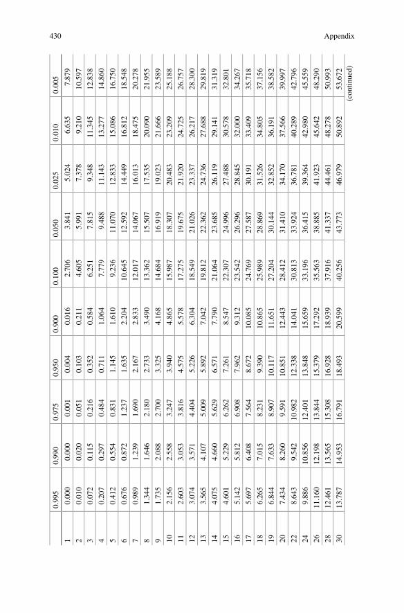
0.99
50.99
00.97
50.95
00.90
00.10
00.05
00.02
50.01
00.00
5
10.00
00.00
00.00
10.00
40.01
62.70
63.84
15.02
46.63
57.87
9
20.01
00.02
00.05
10.10
30.21
14.60
55.99
17.37
89.21
010
.597
30.07
20.11
50.21
60.35
20.58
46.25
17.81
59.34
811
.345
12.838
40.20
70.29
70.48
40.71
11.06
47.77
99.48
811
.143
13.277
14.860
50.41
20.55
40.83
11.14
51.61
09.23
611
.070
12.833
15.086
16.750
60.67
60.87
21.23
71.63
52.20
410
.645
12.592
14.449
16.812
18.548
70.98
91.23
91.69
02.16
72.83
312
.017
14.067
16.013
18.475
20.278
81.34
41.64
62.18
02.73
33.49
013
.362
15.507
17.535
20.090
21.955
91.73
52.08
82.70
03.32
54.16
814
.684
16.919
19.023
21.666
23.589
102.15
62.55
83.24
73.94
04.86
515
.987
18.307
20.483
23.209
25.188
112.60
33.05
33.81
64.57
55.57
817
.275
19.675
21.920
24.725
26.757
123.07
43.57
14.40
45.22
66.30
418
.549
21.026
23.337
26.217
28.300
133.56
54.10
75.00
95.89
27.04
219
.812
22.362
24.736
27.688
29.819
144.07
54.66
05.62
96.57
17.79
021
.064
23.685
26.119
29.141
31.319
154.60
15.22
96.26
27.26
18.54
722
.307
24.996
27.488
30.578
32.801
165.14
25.81
26.90
87.96
29.31
223
.542
26.296
28.845
32.000
34.267
175.69
76.40
87.56
48.67
210
.085
24.769
27.587
30.191
33.409
35.718
186.26
57.01
58.23
19.39
010
.865
25.989
28.869
31.526
34.805
37.156
196.84
47.63
38.90
710
.117
11.651
27.204
30.144
32.852
36.191
38.582
207.43
48.26
09.59
110
.851
12.443
28.412
31.410
34.170
37.566
39.997
228.64
39.54
210
.982
12.338
14.041
30.813
33.924
36.781
40.289
42.796
249.88
610
.856
12.401
13.848
15.659
33.196
36.415
39.364
42.980
45.559
2611
.160
12.198
13.844
15.379
17.292
35.563
38.885
41.923
45.642
48.290
2812
.461
13.565
15.308
16.928
18.939
37.916
41.337
44.461
48.278
50.993
3013
.787
14.953
16.791
18.493
20.599
40.256
43.773
46.979
50.892
53.672
(con
tinued)
430 Appendix
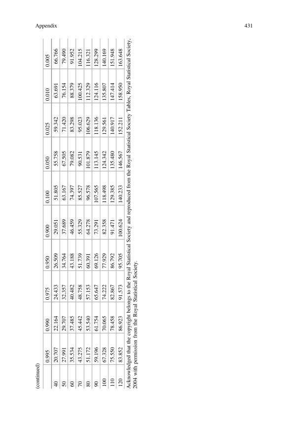
(con
tinued)
0.99
50.99
00.97
50.95
00.90
00.10
00.05
00.02
50.01
00.00
5
4020
.707
22.164
24.433
26.509
29.051
51.805
55.758
59.342
63.691
66.766
5027
.991
29.707
32.357
34.764
37.689
63.167
67.505
71.420
76.154
79.490
6035
.534
37.485
40.482
43.188
46.459
74.397
79.082
83.298
88.379
91.952
7043
.275
45.442
48.758
51.739
55.329
85.527
90.531
95.023
100.42
510
4.21
5
8051
.172
53.540
57.153
60.391
64.278
96.578
101.87
910
6.62
911
2.32
911
6.32
1
9059
.196
61.754
65.647
69.126
73.291
107.56
511
3.14
511
8.13
612
4.11
612
8.29
9
100
67.328
70.065
74.222
77.929
82.358
118.49
812
4.34
212
9.56
113
5.80
714
0.16
9
110
75.550
78.458
82.867
86.792
91.471
129.38
513
5.48
014
0.91
714
7.41
415
1.94
8
120
83.852
86.923
91.573
95.705
100.62
414
0.23
314
6.56
715
2.21
115
8.95
016
3.64
8
Ackno
wledg
edthatthecopy
righ
tbelon
gsto
theRoy
alStatisticalSo
cietyandreprod
uced
from
theRoy
alStatisticalSo
cietyTables,Roy
alStatisticalSo
ciety,
2004
with
perm
ission
from
theRoy
alStatistical
Society.
Appendix 431
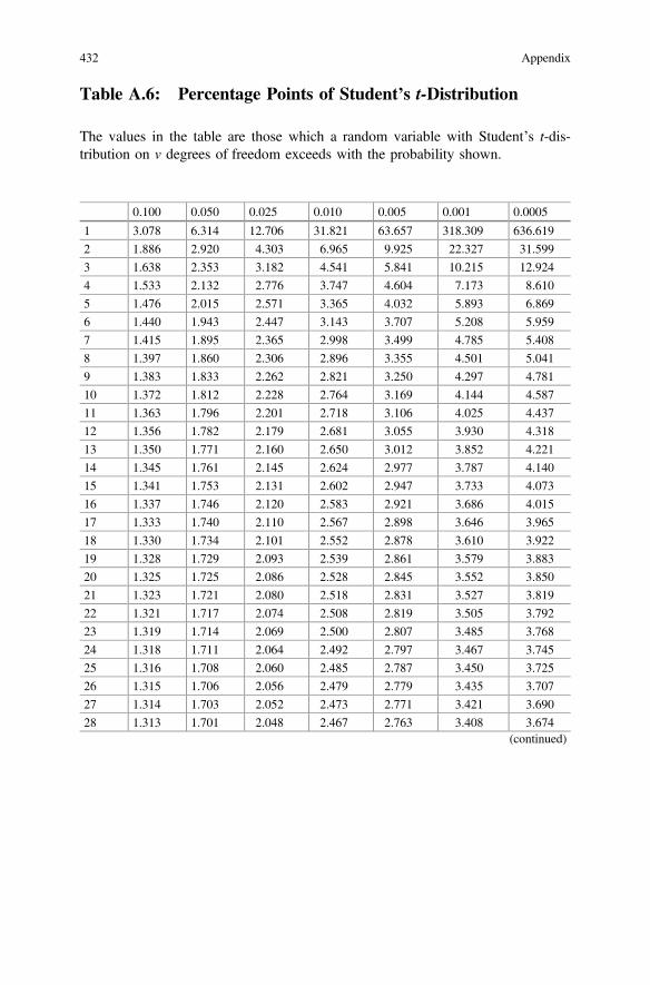
Table A.6: Percentage Points of Student’s t-Distribution
The values in the table are those which a random variable with Student’s t-dis-tribution on v degrees of freedom exceeds with the probability shown.
0.100 0.050 0.025 0.010 0.005 0.001 0.0005
1 3.078 6.314 12.706 31.821 63.657 318.309 636.619
2 1.886 2.920 4.303 6.965 9.925 22.327 31.599
3 1.638 2.353 3.182 4.541 5.841 10.215 12.924
4 1.533 2.132 2.776 3.747 4.604 7.173 8.610
5 1.476 2.015 2.571 3.365 4.032 5.893 6.869
6 1.440 1.943 2.447 3.143 3.707 5.208 5.959
7 1.415 1.895 2.365 2.998 3.499 4.785 5.408
8 1.397 1.860 2.306 2.896 3.355 4.501 5.041
9 1.383 1.833 2.262 2.821 3.250 4.297 4.781
10 1.372 1.812 2.228 2.764 3.169 4.144 4.587
11 1.363 1.796 2.201 2.718 3.106 4.025 4.437
12 1.356 1.782 2.179 2.681 3.055 3.930 4.318
13 1.350 1.771 2.160 2.650 3.012 3.852 4.221
14 1.345 1.761 2.145 2.624 2.977 3.787 4.140
15 1.341 1.753 2.131 2.602 2.947 3.733 4.073
16 1.337 1.746 2.120 2.583 2.921 3.686 4.015
17 1.333 1.740 2.110 2.567 2.898 3.646 3.965
18 1.330 1.734 2.101 2.552 2.878 3.610 3.922
19 1.328 1.729 2.093 2.539 2.861 3.579 3.883
20 1.325 1.725 2.086 2.528 2.845 3.552 3.850
21 1.323 1.721 2.080 2.518 2.831 3.527 3.819
22 1.321 1.717 2.074 2.508 2.819 3.505 3.792
23 1.319 1.714 2.069 2.500 2.807 3.485 3.768
24 1.318 1.711 2.064 2.492 2.797 3.467 3.745
25 1.316 1.708 2.060 2.485 2.787 3.450 3.725
26 1.315 1.706 2.056 2.479 2.779 3.435 3.707
27 1.314 1.703 2.052 2.473 2.771 3.421 3.690
28 1.313 1.701 2.048 2.467 2.763 3.408 3.674(continued)
432 Appendix

Table A.7: Percentage Points of the F-Distribution(Upper 10% Points)
The values in the table are those which a random variable with the F-distribution onv1 and v2 degrees of freedom exceeds with probability 0.10.
If an upper percentage point of the F-distribution on v1 and v2 degrees offreedom is f, then the corresponding lower percentage point of the F-distribution onv2 and v1 degrees of freedom is 1/f
(continued)
0.100 0.050 0.025 0.010 0.005 0.001 0.0005
29 1.311 1.699 2.045 2.462 2.756 3.396 3.659
30 1.310 1.697 2.042 2.457 2.750 3.385 3.646
32 1.309 1.694 2.037 2.449 2.738 3.365 3.622
34 1.307 1.691 2.032 2.441 2.728 3.348 3.601
36 1.306 1.688 2.028 2.434 2.719 3.333 3.582
38 1.304 1.686 2.024 2.429 2.712 3.319 3.566
40 1.303 1.684 2.021 2.423 2.704 3.307 3.551
45 1.301 1.679 2.014 2.412 2.690 3.281 3.520
50 1.299 1.676 2.009 2.403 2.678 3.261 3.496
55 1.297 1.673 2.004 2.396 2.668 3.245 3.476
60 1.296 1.671 2.000 2.390 2.660 3.232 3.460
70 1.294 1.667 1.994 2.381 2.648 3.211 3.435
80 1.292 1.664 1.990 2.374 2.639 3.195 3.416
90 1.291 1.662 1.987 2.368 2.632 3.183 3.402
100 1.290 1.660 1.984 2.364 2.626 3.174 3.390
110 1.289 1.659 1.982 2.361 2.621 3.166 3.381
120 1.289 1.658 1.980 2.358 2.617 3.160 3.373
∞ 1.282 1.645 1.960 2.326 2.576 3.090 3.291
Acknowledged that the copyright belongs to the Royal Statistical Society and reproduced from theRoyal Statistical Society Tables, Royal Statistical Society, 2004 with permission from the RoyalStatistical Society.
Appendix 433

v 2v 1 1
23
45
67
89
1012
1824
∞
139
.86
49.50
53.59
55.83
57.24
58.20
58.91
59.44
59.86
60.19
60.71
61.57
62.00
63.33
28.53
9.00
9.16
9.24
9.29
9.33
9.35
9.37
9.38
9.39
9.41
9.44
9.45
9.49
35.54
5.46
5.39
5.34
5.31
5.28
5.27
5.25
5.24
5.23
5.22
5.19
5.18
5.13
44.54
4.32
4.19
4.11
4.05
4.01
3.98
3.95
3.94
3.92
3.90
3.85
3.83
3.76
54.06
3.78
3.62
3.52
3.45
3.40
3.37
3.34
3.32
3.30
3.27
3.22
3.19
3.10
63.78
3.46
3.29
3.18
3.11
3.05
3.01
2.98
2.96
2.94
2.90
2.85
2.82
2.72
73.59
3.26
3.07
2.96
2.88
2.83
2.78
2.75
2.72
2.70
2.67
2.61
2.58
2.47
83.46
3.11
2.92
2.81
2.73
2.67
2.62
2.59
2.56
2.54
2.50
2.44
2.40
2.29
93.36
3.01
2.81
2.69
2.61
2.55
2.51
2.47
2.44
2.42
2.38
2.31
2.28
2.16
103.29
2.92
2.73
2.61
2.52
2.46
2.41
2.38
2.35
2.32
2.28
2.22
2.18
2.06
113.23
2.86
2.66
2.54
2.45
2.39
2.34
2.30
2.27
2.25
2.21
2.14
2.10
1.97
123.18
2.81
2.61
2.48
2.39
2.33
2.28
2.24
2.21
2.19
2.15
2.08
2.04
1.90
133.14
2.76
2.56
2.43
2.35
2.28
2.23
2.20
2.16
2.14
2.10
2.02
1.98
1.85
143.10
2.73
2.52
2.39
2.31
2.24
2.19
2.15
2.12
2.10
2.05
1.98
1.94
1.80
153.07
2.70
2.49
2.36
2.27
2.21
2.16
2.12
2.09
2.06
2.02
1.94
1.90
1.76
163.05
2.67
2.46
2.33
2.24
2.18
2.13
2.09
2.06
2.03
1.99
1.91
1.87
1.72
173.03
2.64
2.44
2.31
2.22
2.15
2.10
2.06
2.03
2.00
1.96
1.88
1.84
1.69
183.01
2.62
2.42
2.29
2.20
2.13
2.08
2.04
2.00
1.98
1.93
1.85
1.81
1.66
192.99
2.61
2.40
2.27
2.18
2.11
2.06
2.02
1.98
1.96
1.91
1.83
1.79
1.63
202.97
2.59
2.38
2.25
2.16
2.09
2.04
2.00
1.96
1.94
1.89
1.81
1.77
1.61
222.95
2.56
2.35
2.22
2.13
2.06
2.01
1.97
1.93
1.90
1.86
1.78
1.73
1.57
242.93
2.54
2.33
2.19
2.10
2.04
1.98
1.94
1.91
1.88
1.83
1.75
1.70
1.53
262.91
2.52
2.31
2.17
2.08
2.01
1.96
1.92
1.88
1.86
1.81
1.72
1.68
1.50
282.89
2.50
2.29
2.16
2.06
2.00
1.94
1.90
1.87
1.84
1.79
1.70
1.66
1.48
(con
tinued)
434 Appendix

(con
tinued)
v 2v 1 1
23
45
67
89
1012
1824
∞
302.88
2.49
2.28
2.14
2.05
1.98
1.93
1.88
1.85
1.82
1.77
1.69
1.64
1.46
402.84
2.44
2.23
2.09
2.00
1.93
1.87
1.83
1.79
1.76
1.71
1.62
1.57
1.38
502.81
2.41
2.20
2.06
1.97
1.90
1.84
1.80
1.76
1.73
1.68
1.59
1.54
1.33
602.79
2.39
2.18
2.04
1.95
1.87
1.82
1.77
1.74
1.71
1.66
1.56
1.51
1.29
702.78
2.38
2.16
2.03
1.93
1.86
1.80
1.76
1.72
1.69
1.64
1.55
1.49
1.27
802.77
2.37
2.15
2.02
1.92
1.85
1.79
1.75
1.71
1.68
1.63
1.53
1.48
1.24
902.76
2.36
2.15
2.01
1.91
1.84
1.78
1.74
1.70
1.67
1.62
1.52
1.47
1.23
100
2.76
2.36
2.14
2.00
1.91
1.83
1.78
1.73
1.69
1.66
1.61
1.52
1.46
1.21
110
2.75
2.35
2.13
2.00
1.90
1.83
1.77
1.73
1.69
1.66
1.61
1.51
1.45
1.20
120
2.75
2.35
2.13
1.99
1.90
1.82
1.77
1.72
1.68
1.65
1.60
1.50
1.45
1.19
∞2.71
2.30
2.08
1.94
1.85
1.77
1.72
1.67
1.63
1.60
1.55
1.44
1.38
1.00
Ackno
wledg
edthatthecopy
righ
tbelon
gsto
theRoy
alStatisticalSo
cietyandreprod
uced
from
theRoy
alStatisticalSo
cietyTables,Roy
alStatisticalSo
ciety,
2004
with
perm
ission
from
theRoy
alStatistical
Society.
Appendix 435

Table A.7: Percentage Points of the F-Distribution(Upper 5% Points)
The values in the table are those which a random variable with the F-distribution onv1 and v2 degrees of freedom exceeds with probability 0.05.
If an upper percentage point of the F-distribution on v1 and v2 degrees offreedom is f, then the corresponding lower percentage point of the F-distribution onv2 and v1 degrees of freedom is 1/f
436 Appendix
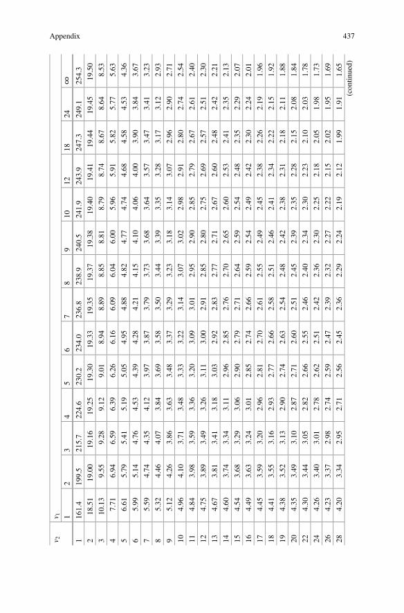
v 2v 1 1
23
45
67
89
1012
1824
∞
116
1.4
199.5
215.7
224.6
230.2
234.0
236.8
238.9
240.5
241.9
243.9
247.3
249.1
254.3
218
.51
19.00
19.16
19.25
19.30
19.33
19.35
19.37
19.38
19.40
19.41
19.44
19.45
19.50
310
.13
9.55
9.28
9.12
9.01
8.94
8.89
8.85
8.81
8.79
8.74
8.67
8.64
8.53
47.71
6.94
6.59
6.39
6.26
6.16
6.09
6.04
6.00
5.96
5.91
5.82
5.77
5.63
56.61
5.79
5.41
5.19
5.05
4.95
4.88
4.82
4.77
4.74
4.68
4.58
4.53
4.36
65.99
5.14
4.76
4.53
4.39
4.28
4.21
4.15
4.10
4.06
4.00
3.90
3.84
3.67
75.59
4.74
4.35
4.12
3.97
3.87
3.79
3.73
3.68
3.64
3.57
3.47
3.41
3.23
85.32
4.46
4.07
3.84
3.69
3.58
3.50
3.44
3.39
3.35
3.28
3.17
3.12
2.93
95.12
4.26
3.86
3.63
3.48
3.37
3.29
3.23
3.18
3.14
3.07
2.96
2.90
2.71
104.96
4.10
3.71
3.48
3.33
3.22
3.14
3.07
3.02
2.98
2.91
2.80
2.74
2.54
114.84
3.98
3.59
3.36
3.20
3.09
3.01
2.95
2.90
2.85
2.79
2.67
2.61
2.40
124.75
3.89
3.49
3.26
3.11
3.00
2.91
2.85
2.80
2.75
2.69
2.57
2.51
2.30
134.67
3.81
3.41
3.18
3.03
2.92
2.83
2.77
2.71
2.67
2.60
2.48
2.42
2.21
144.60
3.74
3.34
3.11
2.96
2.85
2.76
2.70
2.65
2.60
2.53
2.41
2.35
2.13
154.54
3.68
3.29
3.06
2.90
2.79
2.71
2.64
2.59
2.54
2.48
2.35
2.29
2.07
164.49
3.63
3.24
3.01
2.85
2.74
2.66
2.59
2.54
2.49
2.42
2.30
2.24
2.01
174.45
3.59
3.20
2.96
2.81
2.70
2.61
2.55
2.49
2.45
2.38
2.26
2.19
1.96
184.41
3.55
3.16
2.93
2.77
2.66
2.58
2.51
2.46
2.41
2.34
2.22
2.15
1.92
194.38
3.52
3.13
2.90
2.74
2.63
2.54
2.48
2.42
2.38
2.31
2.18
2.11
1.88
204.35
3.49
3.10
2.87
2.71
2.60
2.51
2.45
2.39
2.35
2.28
2.15
2.08
1.84
224.30
3.44
3.05
2.82
2.66
2.55
2.46
2.40
2.34
2.30
2.23
2.10
2.03
1.78
244.26
3.40
3.01
2.78
2.62
2.51
2.42
2.36
2.30
2.25
2.18
2.05
1.98
1.73
264.23
3.37
2.98
2.74
2.59
2.47
2.39
2.32
2.27
2.22
2.15
2.02
1.95
1.69
284.20
3.34
2.95
2.71
2.56
2.45
2.36
2.29
2.24
2.19
2.12
1.99
1.91
1.65
(con
tinued)
Appendix 437
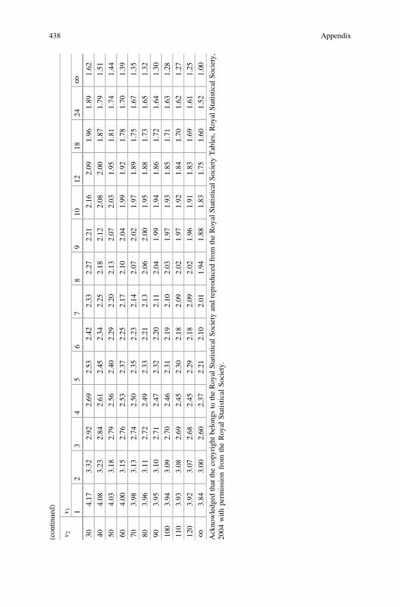
(con
tinued)
v 2v 1 1
23
45
67
89
1012
1824
∞
304.17
3.32
2.92
2.69
2.53
2.42
2.33
2.27
2.21
2.16
2.09
1.96
1.89
1.62
404.08
3.23
2.84
2.61
2.45
2.34
2.25
2.18
2.12
2.08
2.00
1.87
1.79
1.51
504.03
3.18
2.79
2.56
2.40
2.29
2.20
2.13
2.07
2.03
1.95
1.81
1.74
1.44
604.00
3.15
2.76
2.53
2.37
2.25
2.17
2.10
2.04
1.99
1.92
1.78
1.70
1.39
703.98
3.13
2.74
2.50
2.35
2.23
2.14
2.07
2.02
1.97
1.89
1.75
1.67
1.35
803.96
3.11
2.72
2.49
2.33
2.21
2.13
2.06
2.00
1.95
1.88
1.73
1.65
1.32
903.95
3.10
2.71
2.47
2.32
2.20
2.11
2.04
1.99
1.94
1.86
1.72
1.64
1.30
100
3.94
3.09
2.70
2.46
2.31
2.19
2.10
2.03
1.97
1.93
1.85
1.71
1.63
1.28
110
3.93
3.08
2.69
2.45
2.30
2.18
2.09
2.02
1.97
1.92
1.84
1.70
1.62
1.27
120
3.92
3.07
2.68
2.45
2.29
2.18
2.09
2.02
1.96
1.91
1.83
1.69
1.61
1.25
∞3.84
3.00
2.60
2.37
2.21
2.10
2.01
1.94
1.88
1.83
1.75
1.60
1.52
1.00
Ackno
wledg
edthatthecopy
righ
tbelon
gsto
theRoy
alStatisticalSo
cietyandreprod
uced
from
theRoy
alStatisticalSo
cietyTables,Roy
alStatisticalSo
ciety,
2004
with
perm
ission
from
theRoy
alStatistical
Society.
438 Appendix

Table A.7: Percentage Points of the F-Distribution(Upper 2.5% Points)
The values in the table are those which a random variable with the F-distribution onv1 and v2 degrees of freedom exceeds with probability 0.025.
If an upper percentage point of the F-distribution on v1 and v2 degrees offreedom is f, then the corresponding lower percentage point of the F-distribution onv2 and v1 degrees of freedom is 1/f
Appendix 439
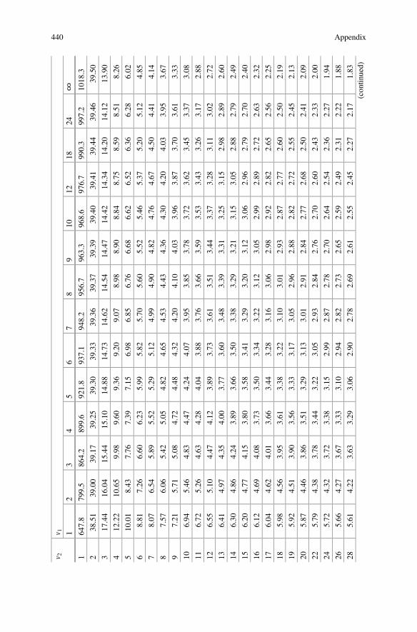
v 2v 1 1
23
45
67
89
1012
1824
∞
164
7.8
799.5
864.2
899.6
921.8
937.1
948.2
956.7
963.3
968.6
976.7
990.3
997.2
1018
.3
238
.51
39.00
39.17
39.25
39.30
39.33
39.36
39.37
39.39
39.40
39.41
39.44
39.46
39.50
317
.44
16.04
15.44
15.10
14.88
14.73
14.62
14.54
14.47
14.42
14.34
14.20
14.12
13.90
412
.22
10.65
9.98
9.60
9.36
9.20
9.07
8.98
8.90
8.84
8.75
8.59
8.51
8.26
510
.01
8.43
7.76
7.39
7.15
6.98
6.85
6.76
6.68
6.62
6.52
6.36
6.28
6.02
68.81
7.26
6.60
6.23
5.99
5.82
5.70
5.60
5.52
5.46
5.37
5.20
5.12
4.85
78.07
6.54
5.89
5.52
5.29
5.12
4.99
4.90
4.82
4.76
4.67
4.50
4.41
4.14
87.57
6.06
5.42
5.05
4.82
4.65
4.53
4.43
4.36
4.30
4.20
4.03
3.95
3.67
97.21
5.71
5.08
4.72
4.48
4.32
4.20
4.10
4.03
3.96
3.87
3.70
3.61
3.33
106.94
5.46
4.83
4.47
4.24
4.07
3.95
3.85
3.78
3.72
3.62
3.45
3.37
3.08
116.72
5.26
4.63
4.28
4.04
3.88
3.76
3.66
3.59
3.53
3.43
3.26
3.17
2.88
126.55
5.10
4.47
4.12
3.89
3.73
3.61
3.51
3.44
3.37
3.28
3.11
3.02
2.72
136.41
4.97
4.35
4.00
3.77
3.60
3.48
3.39
3.31
3.25
3.15
2.98
2.89
2.60
146.30
4.86
4.24
3.89
3.66
3.50
3.38
3.29
3.21
3.15
3.05
2.88
2.79
2.49
156.20
4.77
4.15
3.80
3.58
3.41
3.29
3.20
3.12
3.06
2.96
2.79
2.70
2.40
166.12
4.69
4.08
3.73
3.50
3.34
3.22
3.12
3.05
2.99
2.89
2.72
2.63
2.32
176.04
4.62
4.01
3.66
3.44
3.28
3.16
3.06
2.98
2.92
2.82
2.65
2.56
2.25
185.98
4.56
3.95
3.61
3.38
3.22
3.10
3.01
2.93
2.87
2.77
2.60
2.50
2.19
195.92
4.51
3.90
3.56
3.33
3.17
3.05
2.96
2.88
2.82
2.72
2.55
2.45
2.13
205.87
4.46
3.86
3.51
3.29
3.13
3.01
2.91
2.84
2.77
2.68
2.50
2.41
2.09
225.79
4.38
3.78
3.44
3.22
3.05
2.93
2.84
2.76
2.70
2.60
2.43
2.33
2.00
245.72
4.32
3.72
3.38
3.15
2.99
2.87
2.78
2.70
2.64
2.54
2.36
2.27
1.94
265.66
4.27
3.67
3.33
3.10
2.94
2.82
2.73
2.65
2.59
2.49
2.31
2.22
1.88
285.61
4.22
3.63
3.29
3.06
2.90
2.78
2.69
2.61
2.55
2.45
2.27
2.17
1.83
(con
tinued)
440 Appendix

(con
tinued)
v 2v 1 1
23
45
67
89
1012
1824
∞
305.57
4.18
3.59
3.25
3.03
2.87
2.75
2.65
2.57
2.51
2.41
2.23
2.14
1.79
405.42
4.05
3.46
3.13
2.90
2.74
2.62
2.53
2.45
2.39
2.29
2.11
2.01
1.64
505.34
3.97
3.39
3.05
2.83
2.67
2.55
2.46
2.38
2.32
2.22
2.03
1.93
1.55
605.29
3.93
3.34
3.01
2.79
2.63
2.51
2.41
2.33
2.27
2.17
1.98
1.88
1.48
705.25
3.89
3.31
2.97
2.75
2.59
2.47
2.38
2.30
2.24
2.14
1.95
1.85
1.44
805.22
3.86
3.28
2.95
2.73
2.57
2.45
2.35
2.28
2.21
2.11
1.92
1.82
1.40
905.20
3.84
3.26
2.93
2.71
2.55
2.43
2.34
2.26
2.19
2.09
1.91
1.80
1.37
100
5.18
3.83
3.25
2.92
2.70
2.54
2.42
2.32
2.24
2.18
2.08
1.89
1.78
1.35
110
5.16
3.82
3.24
2.90
2.68
2.53
2.40
2.31
2.23
2.17
2.07
1.88
1.77
1.33
120
5.15
3.80
3.23
2.89
2.67
2.52
2.39
2.30
2.22
2.16
2.05
1.87
1.76
1.31
∞5.02
3.69
3.12
2.79
2.57
2.41
2.29
2.19
2.11
2.05
1.94
1.75
1.64
1.00
Ackno
wledg
edthatthecopy
righ
tbelon
gsto
theRoy
alStatisticalSo
cietyandreprod
uced
from
theRoy
alStatisticalSo
cietyTables,Roy
alStatisticalSo
ciety,
2004
with
perm
ission
from
theRoy
alStatistical
Society.
Appendix 441

Table A.7: Percentage Points of the F-Distribution(Upper 1% Points)
The values in the table are those which a random variable with the F-distribution onv1 and v2 degrees of freedom exceeds with probability 0.01.
If an upper percentage point of the F-distribution on v1 and v2 degrees offreedom is f, then the corresponding lower percentage point of the F-distribution onv2 and v1 degrees of freedom is 1/f
442 Appendix

v 2v 1 1
23
45
67
89
1012
1824
∞
140
5250
0054
0356
2557
6458
5959
2859
8160
2260
5661
0661
9262
3563
66
298
.50
99.00
99.17
99.25
99.30
99.33
99.36
99.37
99.39
99.40
99.42
99.44
99.46
99.50
334
.12
30.82
29.46
28.71
28.24
27.91
27.67
27.49
27.34
27.23
27.05
26.75
26.60
26.13
421
.20
18.00
16.69
15.98
15.52
15.21
14.98
14.80
14.66
14.55
14.37
14.08
13.93
13.46
516
.26
13.27
12.06
11.39
10.97
10.67
10.46
10.29
10.16
10.05
9.89
9.61
9.47
9.02
613
.74
10.93
9.78
9.15
8.75
8.47
8.26
8.10
7.98
7.87
7.72
7.45
7.31
6.88
712
.25
9.55
8.45
7.85
7.46
7.19
6.99
6.84
6.72
6.62
6.47
6.21
6.07
5.65
811
.26
8.65
7.59
7.01
6.63
6.37
6.18
6.03
5.91
5.81
5.67
5.41
5.28
4.86
910
.56
8.02
6.99
6.42
6.06
5.80
5.61
5.47
5.35
5.26
5.11
4.86
4.73
4.31
1010
.04
7.56
6.55
5.99
5.64
5.39
5.20
5.06
4.94
4.85
4.71
4.46
4.33
3.91
119.65
7.21
6.22
5.67
5.32
5.07
4.89
4.74
4.63
4.54
4.40
4.15
4.02
3.60
129.33
6.93
5.95
5.41
5.06
4.82
4.64
4.50
4.39
4.30
4.16
3.91
3.78
3.36
139.07
6.70
5.74
5.21
4.86
4.62
4.44
4.30
4.19
4.10
3.96
3.72
3.59
3.17
148.86
6.51
5.56
5.04
4.70
4.46
4.28
4.14
4.03
3.94
3.80
3.56
3.43
3.00
158.68
6.36
5.42
4.89
4.56
4.32
4.14
4.00
3.90
3.81
3.67
3.42
3.29
2.87
168.53
6.23
5.29
4.77
4.44
4.20
4.03
3.89
3.78
3.69
3.55
3.31
3.18
2.75
178.40
6.11
5.18
4.67
4.34
4.10
3.93
3.79
3.68
3.59
3.46
3.21
3.08
2.65
188.29
6.01
5.09
4.58
4.25
4.01
3.84
3.71
3.60
3.51
3.37
3.13
3.00
2.57
198.19
5.93
5.01
4.50
4.17
3.94
3.77
3.63
3.52
3.43
3.30
3.05
2.92
2.49
208.10
5.85
4.94
4.43
4.10
3.87
3.70
3.56
3.46
3.37
3.23
2.99
2.86
2.42
227.95
5.72
4.82
4.31
3.99
3.76
3.59
3.45
3.35
3.26
3.12
2.88
2.75
2.31
247.82
5.61
4.72
4.22
3.90
3.67
3.50
3.36
3.26
3.17
3.03
2.79
2.66
2.21
267.72
5.53
4.64
4.14
3.82
3.59
3.42
3.29
3.18
3.09
2.96
2.71
2.59
2.13
287.64
5.45
4.57
4.07
3.75
3.53
3.36
3.23
3.12
3.03
2.90
2.65
2.52
2.06
(con
tinued)
Appendix 443

(con
tinued)
v 2v 1 1
23
45
67
89
1012
1824
∞
307.56
5.39
4.51
4.02
3.70
3.47
3.30
3.17
3.07
2.98
2.84
2.60
2.47
2.01
407.31
5.18
4.31
3.83
3.51
3.29
3.12
2.99
2.89
2.80
2.67
2.42
2.29
1.80
507.17
5.06
4.20
3.72
3.41
3.19
3.02
2.89
2.79
2.70
2.56
2.32
2.18
1.68
607.08
4.98
4.13
3.65
3.34
3.12
2.95
2.82
2.72
2.63
2.50
2.25
2.12
1.60
707.01
4.92
4.07
3.60
3.29
3.07
2.91
2.78
2.67
2.59
2.45
2.20
2.07
1.54
806.96
4.88
4.04
3.56
3.25
3.04
2.87
2.74
2.64
2.55
2.42
2.17
2.03
1.49
906.92
4.85
4.01
3.54
3.23
3.01
2.85
2.71
2.61
2.52
2.39
2.14
2.00
1.46
100
6.89
4.82
3.98
3.51
3.21
2.99
2.82
2.69
2.59
2.50
2.37
2.12
1.98
1.43
110
6.87
4.80
3.96
3.50
3.19
2.97
2.81
2.68
2.57
2.49
2.35
2.10
1.97
1.40
120
6.85
4.79
3.95
3.48
3.17
2.96
2.79
2.66
2.56
2.47
2.34
2.09
1.95
1.38
∞6.63
4.61
3.78
3.32
3.02
2.80
2.64
2.51
2.41
2.32
2.19
1.93
1.79
1.00
Ackno
wledg
edthatthecopy
righ
tbelon
gsto
theRoy
alStatisticalSo
cietyandreprod
uced
from
theRoy
alStatisticalSo
cietyTables,Roy
alStatisticalSo
ciety,
2004
with
perm
ission
from
theRoy
alStatistical
Society.
444 Appendix

Table A.7: Percentage Points of the F-Distribution(Upper 0.5% Points)
The values in the table are those which a random variable with the F-distribution onv1 and v2 degrees of freedom exceeds with probability 0.005.
If an upper percentage point of the F-distribution on v1 and v2 degrees offreedom is f, then the corresponding lower percentage point of the F-distribution onv2 and v1 degrees of freedom is 1/f
Appendix 445

v 2v 1 1
23
45
67
89
1012
1824
∞
116
211
2000
021
615
2250
023
056
2343
723
715
2392
524
091
2422
424
426
2476
724
940
2546
4
219
8.5
199.0
199.2
199.3
199.3
199.3
199.4
199.4
199.4
199.4
199.4
199.4
199.5
199.5
355
.55
49.80
47.47
46.19
45.39
44.84
44.43
44.13
43.88
43.69
43.39
42.88
42.62
41.83
431
.33
26.28
24.26
23.15
22.46
21.97
21.62
21.35
21.14
20.97
20.70
20.26
20.03
19.32
522
.78
18.31
16.53
15.56
14.94
14.51
14.20
13.96
13.77
13.62
13.38
12.98
12.78
12.14
618
.63
14.54
12.92
12.03
11.46
11.07
10.79
10.57
10.39
10.25
10.03
9.66
9.47
8.88
716
.24
12.40
10.88
10.05
9.52
9.16
8.89
8.68
8.51
8.38
8.18
7.83
7.64
7.08
814
.69
11.04
9.60
8.81
8.30
7.95
7.69
7.50
7.34
7.21
7.01
6.68
6.50
5.95
913
.61
10.11
8.72
7.96
7.47
7.13
6.88
6.69
6.54
6.42
6.23
5.90
5.73
5.19
1012
.83
9.43
8.08
7.34
6.87
6.54
6.30
6.12
5.97
5.85
5.66
5.34
5.17
4.64
1112
.23
8.91
7.60
6.88
6.42
6.10
5.86
5.68
5.54
5.42
5.24
4.92
4.76
4.23
1211
.75
8.51
7.23
6.52
6.07
5.76
5.52
5.35
5.20
5.09
4.91
4.59
4.43
3.90
1311
.37
8.19
6.93
6.23
5.79
5.48
5.25
5.08
4.94
4.82
4.64
4.33
4.17
3.65
1411
.06
7.92
6.68
6.00
5.56
5.26
5.03
4.86
4.72
4.60
4.43
4.12
3.96
3.44
1510
.80
7.70
6.48
5.80
5.37
5.07
4.85
4.67
4.54
4.42
4.25
3.95
3.79
3.26
1610
.58
7.51
6.30
5.64
5.21
4.91
4.69
4.52
4.38
4.27
4.10
3.80
3.64
3.11
1710
.38
7.35
6.16
5.50
5.07
4.78
4.56
4.39
4.25
4.14
3.97
3.67
3.51
2.98
1810
.22
7.21
6.03
5.37
4.96
4.66
4.44
4.28
4.14
4.03
3.86
3.56
3.40
2.87
1910
.07
7.09
5.92
5.27
4.85
4.56
4.34
4.18
4.04
3.93
3.76
3.46
3.31
2.78
209.94
6.99
5.82
5.17
4.76
4.47
4.26
4.09
3.96
3.85
3.68
3.38
3.22
2.69
229.73
6.81
5.65
5.02
4.61
4.32
4.11
3.94
3.81
3.70
3.54
3.24
3.08
2.55
249.55
6.66
5.52
4.89
4.49
4.20
3.99
3.83
3.69
3.59
3.42
3.12
2.97
2.43
269.41
6.54
5.41
4.79
4.38
4.10
3.89
3.73
3.60
3.49
3.33
3.03
2.87
2.33
289.28
6.44
5.32
4.70
4.30
4.02
3.81
3.65
3.52
3.41
3.25
2.95
2.79
2.25
(con
tinued)
446 Appendix

(con
tinued)
v 2v 1 1
23
45
67
89
1012
1824
∞
309.18
6.35
5.24
4.62
4.23
3.95
3.74
3.58
3.45
3.34
3.18
2.89
2.73
2.18
408.83
6.07
4.98
4.37
3.99
3.71
3.51
3.35
3.22
3.12
2.95
2.66
2.50
1.93
508.63
5.90
4.83
4.23
3.85
3.58
3.38
3.22
3.09
2.99
2.82
2.53
2.37
1.79
608.49
5.79
4.73
4.14
3.76
3.49
3.29
3.13
3.01
2.90
2.74
2.45
2.29
1.69
708.40
5.72
4.66
4.08
3.70
3.43
3.23
3.08
2.95
2.85
2.68
2.39
2.23
1.62
808.33
5.67
4.61
4.03
3.65
3.39
3.19
3.03
2.91
2.80
2.64
2.35
2.19
1.56
908.28
5.62
4.57
3.99
3.62
3.35
3.15
3.00
2.87
2.77
2.61
2.32
2.15
1.52
100
8.24
5.59
4.54
3.96
3.59
3.33
3.13
2.97
2.85
2.74
2.58
2.29
2.13
1.49
110
8.21
5.56
4.52
3.94
3.57
3.30
3.11
2.95
2.83
2.72
2.56
2.27
2.11
1.46
120
8.18
5.54
4.50
3.92
3.55
3.28
3.09
2.93
2.81
2.71
2.54
2.25
2.09
1.43
∞7.88
5.30
4.28
3.72
3.35
3.09
2.90
2.74
2.62
2.52
2.36
2.06
1.90
1.00
Ackno
wledg
edthatthecopy
righ
tbelon
gsto
theRoy
alStatisticalSo
cietyandreprod
uced
from
theRoy
alStatisticalSo
cietyTables,Roy
alStatisticalSo
ciety,
2004
with
perm
ission
from
theRoy
alStatistical
Society.
Appendix 447

Table A.7: Percentage Points of the F-Distribution(Upper 0.1% Points)
The values in the table are those which a random variable with the F-distribution onv1 and v2 degrees of freedom exceeds with probability 0.001.
Note: All percentage points in the row for v2 ¼ 1 must be multiplied by 100; forexample, the percentage point for F8,1 is 598100 (to 4 significant figures)
If an upper percentage point of the F-distribution on v1 and v2 degrees offreedom is f, then the corresponding lower percentage point of the F-distribution onv2 and v1 degrees of freedom is 1/f
448 Appendix

v 2v 1 1
23
45
67
89
1012
1824
∞
140
53*
5000
*54
04*
5625
*57
64*
5859
*59
29*
5981
*60
23*
6056
*61
07*
6192
*62
35*
6366
*
299
8.5
999.0
999.2
999.3
999.3
999.3
999.4
999.4
999.4
999.4
999.4
999.4
999.5
999.5
316
7.0
148.5
141.1
137.1
134.6
132.8
131.6
130.6
129.9
129.2
128.3
126.7
125.9
123.5
474
.14
61.25
56.18
53.44
51.71
50.53
49.66
49.00
48.47
48.05
47.41
46.32
45.77
44.05
547
.18
37.12
33.20
31.09
29.75
28.83
28.16
27.65
27.24
26.92
26.42
25.57
25.13
23.79
635
.51
27.00
23.70
21.92
20.80
20.03
19.46
19.03
18.69
18.41
17.99
17.27
16.90
15.75
729
.25
21.69
18.77
17.20
16.21
15.52
15.02
14.63
14.33
14.08
13.71
13.06
12.73
11.70
825
.41
18.49
15.83
14.39
13.48
12.86
12.40
12.05
11.77
11.54
11.19
10.60
10.30
9.33
922
.86
16.39
13.90
12.56
11.71
11.13
10.70
10.37
10.11
9.89
9.57
9.01
8.72
7.81
1021
.04
14.91
12.55
11.28
10.48
9.93
9.52
9.20
8.96
8.75
8.45
7.91
7.64
6.76
1119
.69
13.81
11.56
10.35
9.58
9.05
8.66
8.35
8.12
7.92
7.63
7.11
6.85
6.00
1218
.64
12.97
10.80
9.63
8.89
8.38
8.00
7.71
7.48
7.29
7.00
6.51
6.25
5.42
1317
.82
12.31
10.21
9.07
8.35
7.86
7.49
7.21
6.98
6.80
6.52
6.03
5.78
4.97
1417
.14
11.78
9.73
8.62
7.92
7.44
7.08
6.80
6.58
6.40
6.13
5.66
5.41
4.60
1516
.59
11.34
9.34
8.25
7.57
7.09
6.74
6.47
6.26
6.08
5.81
5.35
5.10
4.31
1616
.12
10.97
9.01
7.94
7.27
6.80
6.46
6.19
5.98
5.81
5.55
5.09
4.85
4.06
1715
.72
10.66
8.73
7.68
7.02
6.56
6.22
5.96
5.75
5.58
5.32
4.87
4.63
3.85
1815
.38
10.39
8.49
7.46
6.81
6.35
6.02
5.76
5.56
5.39
5.13
4.68
4.45
3.67
1915
.08
10.16
8.28
7.27
6.62
6.18
5.85
5.59
5.39
5.22
4.97
4.52
4.29
3.51
2014
.82
9.95
8.10
7.10
6.46
6.02
5.69
5.44
5.24
5.08
4.82
4.38
4.15
3.38
2214
.38
9.61
7.80
6.81
6.19
5.76
5.44
5.19
4.99
4.83
4.58
4.15
3.92
3.15
2414
.03
9.34
7.55
6.59
5.98
5.55
5.23
4.99
4.80
4.64
4.39
3.96
3.74
2.97
2613
.74
9.12
7.36
6.41
5.80
5.38
5.07
4.83
4.64
4.48
4.24
3.81
3.59
2.82
2813
.50
8.93
7.19
6.25
5.66
5.24
4.93
4.69
4.50
4.35
4.11
3.69
3.46
2.69
(con
tinued)
Appendix 449

(con
tinued)
v 2v 1 1
23
45
67
89
1012
1824
∞
3013
.29
8.77
7.05
6.12
5.53
5.12
4.82
4.58
4.39
4.24
4.00
3.58
3.36
2.59
4012
.61
8.25
6.59
5.70
5.13
4.73
4.44
4.21
4.02
3.87
3.64
3.23
3.01
2.23
5012
.22
7.96
6.34
5.46
4.90
4.51
4.22
4.00
3.82
3.67
3.44
3.04
2.82
2.03
6011
.97
7.77
6.17
5.31
4.76
4.37
4.09
3.86
3.69
3.54
3.32
2.91
2.69
1.89
7011
.80
7.64
6.06
5.20
4.66
4.28
3.99
3.77
3.60
3.45
3.23
2.83
2.61
1.79
8011
.67
7.54
5.97
5.12
4.58
4.20
3.92
3.70
3.53
3.39
3.16
2.76
2.54
1.72
9011
.57
7.47
5.91
5.06
4.53
4.15
3.87
3.65
3.48
3.34
3.11
2.71
2.50
1.66
100
11.50
7.41
5.86
5.02
4.48
4.11
3.83
3.61
3.44
3.30
3.07
2.68
2.46
1.62
110
11.43
7.36
5.82
4.98
4.45
4.07
3.79
3.58
3.41
3.26
3.04
2.65
2.43
1.58
120
11.38
7.32
5.78
4.95
4.42
4.04
3.77
3.55
3.38
3.24
3.02
2.62
2.40
1.54
∞10
.83
6.91
5.42
4.62
4.10
3.74
3.47
3.27
3.10
2.96
2.74
2.35
2.13
1.00
Ackno
wledg
edthatthecopy
righ
tbelon
gsto
theRoy
alStatisticalSo
cietyandreprod
uced
from
theRoy
alStatisticalSo
cietyTables,Roy
alStatisticalSo
ciety,
2004
with
perm
ission
from
theRoy
alStatistical
Society.
450 Appendix
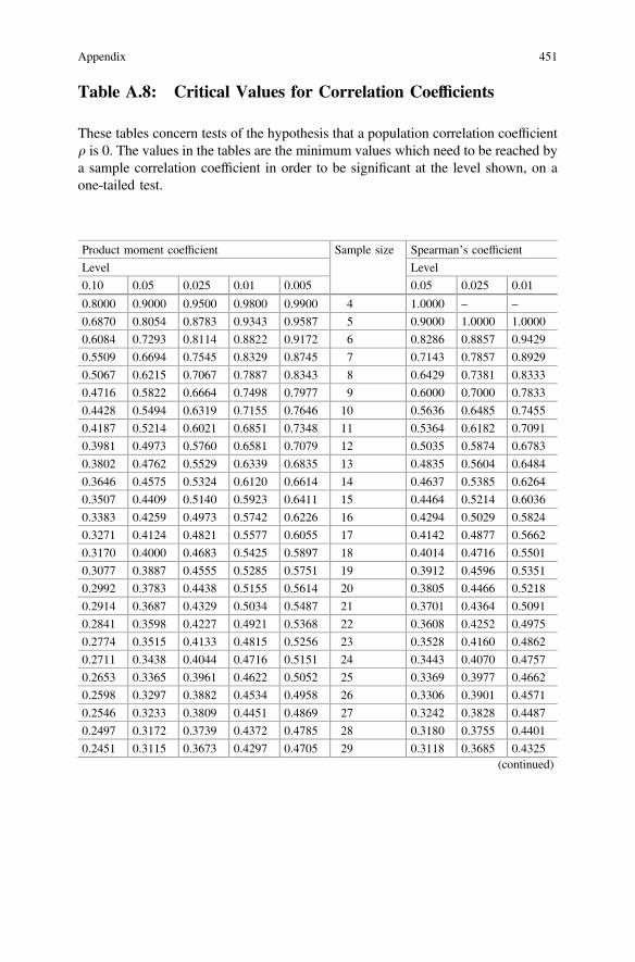
Table A.8: Critical Values for Correlation Coefficients
These tables concern tests of the hypothesis that a population correlation coefficientq is 0. The values in the tables are the minimum values which need to be reached bya sample correlation coefficient in order to be significant at the level shown, on aone-tailed test.
Product moment coefficient Sample size Spearman’s coefficient
Level Level
0.10 0.05 0.025 0.01 0.005 0.05 0.025 0.01
0.8000 0.9000 0.9500 0.9800 0.9900 4 1.0000 – –
0.6870 0.8054 0.8783 0.9343 0.9587 5 0.9000 1.0000 1.0000
0.6084 0.7293 0.8114 0.8822 0.9172 6 0.8286 0.8857 0.9429
0.5509 0.6694 0.7545 0.8329 0.8745 7 0.7143 0.7857 0.8929
0.5067 0.6215 0.7067 0.7887 0.8343 8 0.6429 0.7381 0.8333
0.4716 0.5822 0.6664 0.7498 0.7977 9 0.6000 0.7000 0.7833
0.4428 0.5494 0.6319 0.7155 0.7646 10 0.5636 0.6485 0.7455
0.4187 0.5214 0.6021 0.6851 0.7348 11 0.5364 0.6182 0.7091
0.3981 0.4973 0.5760 0.6581 0.7079 12 0.5035 0.5874 0.6783
0.3802 0.4762 0.5529 0.6339 0.6835 13 0.4835 0.5604 0.6484
0.3646 0.4575 0.5324 0.6120 0.6614 14 0.4637 0.5385 0.6264
0.3507 0.4409 0.5140 0.5923 0.6411 15 0.4464 0.5214 0.6036
0.3383 0.4259 0.4973 0.5742 0.6226 16 0.4294 0.5029 0.5824
0.3271 0.4124 0.4821 0.5577 0.6055 17 0.4142 0.4877 0.5662
0.3170 0.4000 0.4683 0.5425 0.5897 18 0.4014 0.4716 0.5501
0.3077 0.3887 0.4555 0.5285 0.5751 19 0.3912 0.4596 0.5351
0.2992 0.3783 0.4438 0.5155 0.5614 20 0.3805 0.4466 0.5218
0.2914 0.3687 0.4329 0.5034 0.5487 21 0.3701 0.4364 0.5091
0.2841 0.3598 0.4227 0.4921 0.5368 22 0.3608 0.4252 0.4975
0.2774 0.3515 0.4133 0.4815 0.5256 23 0.3528 0.4160 0.4862
0.2711 0.3438 0.4044 0.4716 0.5151 24 0.3443 0.4070 0.4757
0.2653 0.3365 0.3961 0.4622 0.5052 25 0.3369 0.3977 0.4662
0.2598 0.3297 0.3882 0.4534 0.4958 26 0.3306 0.3901 0.4571
0.2546 0.3233 0.3809 0.4451 0.4869 27 0.3242 0.3828 0.4487
0.2497 0.3172 0.3739 0.4372 0.4785 28 0.3180 0.3755 0.4401
0.2451 0.3115 0.3673 0.4297 0.4705 29 0.3118 0.3685 0.4325(continued)
Appendix 451

Table A.9: Random Digits
(continued)
Product moment coefficient Sample size Spearman’s coefficient
Level Level
0.10 0.05 0.025 0.01 0.005 0.05 0.025 0.01
0.2407 0.3061 0.3610 0.4226 0.4629 30 0.3063 0.3624 0.4251
0.2070 0.2638 0.3120 0.3665 0.4026 40 0.2640 0.3128 0.3681
0.1843 0.2353 0.2787 0.3281 0.3610 50 0.2353 0.2791 0.3293
0.1678 0.2144 0.2542 0.2997 0.3301 60 0.2144 0.2545 0.3005
0.1550 0.1982 0.2352 0.2776 0.3060 70 0.1982 0.2354 0.2782
0.1448 0.1852 0.2199 0.2597 0.2864 80 0.1852 0.2201 0.2602
0.1364 0.1745 0.2072 0.2449 0.2702 90 0.1745 0.2074 0.2453
0.1292 0.1654 0.1966 0.2324 0.2565 100 0.1654 0.1967 0.2327
Acknowledged that the copyright belongs to the Royal Statistical Society and reproduced from theRoyal Statistical Society Tables, Royal Statistical Society, 2004 with permission from the RoyalStatistical Society.
86 13 84 10 07 30 39 05 97 96 88 07 37 26 04 89 13 48 19 20
60 78 48 12 99 47 09 46 91 33 17 21 03 94 79 00 08 50 40 16
78 48 06 37 82 26 01 06 64 65 94 41 17 26 74 66 61 93 24 97
80 56 90 79 66 94 18 40 97 79 93 20 41 51 25 04 20 71 76 04
99 09 39 25 66 31 70 56 30 15 52 17 87 55 31 11 10 68 98 23
56 32 32 72 91 65 97 36 56 61 12 79 95 17 57 16 53 58 96 36
66 02 49 93 97 44 99 15 56 86 80 57 11 78 40 23 58 40 86 14
31 77 53 94 05 93 56 14 71 23 60 46 05 33 23 72 93 10 81 23
98 79 72 43 14 76 54 77 66 29 84 09 88 56 75 86 41 67 04 42
50 97 92 15 10 01 57 01 87 33 73 17 70 18 40 21 24 20 66 62
90 51 94 50 12 48 88 95 09 34 09 30 22 27 25 56 40 76 01 59
31 99 52 24 13 43 27 88 11 39 41 65 00 84 13 06 31 79 74 97
22 96 23 34 46 12 67 11 48 06 99 24 14 83 78 37 65 73 39 47
06 84 55 41 27 06 74 59 14 29 20 14 45 75 31 16 05 41 22 96
08 64 89 30 25 25 71 35 33 31 04 56 12 67 03 74 07 16 49 32
86 87 62 43 15 11 76 49 79 13 78 80 93 89 09 57 07 14 40 74
94 44 97 13 77 04 35 02 12 76 60 91 93 40 81 06 85 85 72 84
63 25 55 14 66 47 99 90 02 90 83 43 16 01 19 69 11 78 87 16
11 22 83 98 15 21 18 57 53 42 91 91 26 52 89 13 86 00 47 61
01 70 10 83 94 71 13 67 11 12 36 54 53 32 90 43 79 01 95 15
Acknowledged that the copyright belongs to the Royal Statistical Society and reproduced from theRoyal Statistical Society Tables, Royal Statistical Society, 2004 with permission from the RoyalStatistical Society.
452 Appendix
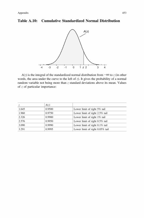
Table A.10: Cumulative Standardized Normal Distribution
A(z)
-4 -3 -2 -1 0 1 z 2 3 4
A(z) is the integral of the standardized normal distribution from −∞ to z (in otherwords, the area under the curve to the left of z). It gives the probability of a normalrandom variable not being more than z standard deviations above its mean. Valuesof z of particular importance:
z A(z)
1.645 0.9500 Lower limit of right 5% tail
1.960 0.9750 Lower limit of right 2.5% tail
2.326 0.9900 Lower limit of right 1% tail
2.576 0.9950 Lower limit of right 0.5% tail
3.090 0.9990 Lower limit of right 0.1% tail
3.291 0.9995 Lower limit of right 0.05% tail
Appendix 453

z0.00
0.01
0.02
0.03
0.04
0.05
0.06
0.07
0.08
0.09
0.0
0.50
000.50
400.50
800.51
200.51
600.51
990.52
390.52
790.53
190.53
59
0.1
0.53
980.54
380.54
780.55
170.55
570.55
960.56
360.56
750.57
140.57
53
0.2
0.57
930.58
320.58
710.59
100.59
480.59
870.60
260.60
640.61
030.61
41
0.3
0.61
790.62
170.62
550.62
930.63
310.63
680.64
060.64
430.64
800.65
17
0.4
0.65
540.65
910.66
280.66
640.67
000.67
360.67
720.68
080.68
440.68
79
0.5
0.69
150.69
500.69
850.70
190.70
540.70
880.71
230.71
570.71
900.72
24
0.6
0.72
570.72
910.73
240.73
570.73
890.74
220.74
540.74
860.75
170.75
49
0.7
0.75
800.76
110.76
420.76
730.77
040.77
340.77
640.77
940.78
230.78
52
0.8
0.78
810.79
100.79
390.79
670.79
950.80
230.80
510.80
780.81
060.81
33
0.9
0.81
590.81
860.82
120.82
380.82
640.82
890.83
150.83
400.83
650.83
89
1.0
0.84
130.84
380.84
610.84
850.85
080.85
310.85
540.85
770.85
990.86
21
1.1
0.86
430.86
650.86
860.87
080.87
290.87
490.87
700.87
900.88
100.88
30
1.2
0.88
490.88
690.88
880.89
070.89
250.89
440.89
620.89
800.89
970.90
15
1.3
0.90
320.90
490.90
660.90
820.90
990.91
150.91
310.91
470.91
620.91
77
1.4
0.91
920.92
070.92
220.92
360.92
510.92
650.92
790.92
920.93
060.93
19
1.5
0.93
320.93
450.93
570.93
700.93
820.93
940.94
060.94
180.94
290.94
41
1.6
0.94
520.94
630.94
740.94
840.94
950.95
050.95
150.95
250.95
350.95
45
1.7
0.95
540.95
640.95
730.95
820.95
910.95
990.96
080.96
160.96
250.96
33
1.8
0.96
410.96
490.96
560.96
640.96
710.96
780.96
860.96
930.96
990.97
06
1.9
0.97
130.97
190.97
260.97
320.97
380.97
440.97
500.97
560.97
610.97
67
2.0
0.97
720.97
780.97
830.97
880.97
930.97
980.98
030.98
080.98
120.98
17
2.1
0.98
210.98
260.98
300.98
340.98
380.98
420.98
460.98
500.98
540.98
57
2.2
0.98
610.98
640.98
680.98
710.98
750.98
780.98
810.98
840.98
870.98
90
2.3
0.98
930.98
960.98
980.99
010.99
040.99
060.99
090.99
110.99
130.99
16
2.4
0.99
180.99
200.99
220.99
250.99
270.99
290.99
310.99
320.99
340.99
36(con
tinued)
454 Appendix

(con
tinued)
z0.00
0.01
0.02
0.03
0.04
0.05
0.06
0.07
0.08
0.09
2.5
0.99
380.99
400.99
410.99
430.99
450.99
460.99
480.99
490.99
510.99
52
2.6
0.99
530.99
550.99
560.99
570.99
590.99
600.99
610.99
620.99
630.99
64
2.7
0.99
650.99
660.99
670.99
680.99
690.99
700.99
710.99
720.99
730.99
74
2.8
0.99
740.99
750.99
760.99
770.99
770.99
780.99
790.99
790.99
800.99
81
2.9
0.99
810.99
820.99
820.99
830.99
840.99
840.99
850.99
850.99
860.99
86
3.0
0.99
870.99
870.99
870.99
880.99
880.99
890.99
890.99
890.99
900.99
90
3.1
0.99
900.99
910.99
910.99
910.99
920.99
920.99
920.99
920.99
930.99
93
3.2
0.99
930.99
930.99
940.99
940.99
940.99
940.99
940.99
950.99
950.99
95
3.3
0.99
950.99
950.99
950.99
960.99
960.99
960.99
960.99
960.99
960.99
97
3.4
0.99
970.99
970.99
970.99
970.99
970.99
970.99
970.99
970.99
970.99
98
3.5
0.99
980.99
980.99
980.99
980.99
980.99
980.99
980.99
980.99
980.99
98
3.6
0.99
980.99
980.99
99
Reprodu
cedwith
perm
ission
from
C.Dou
gherty
2001
,20
02(c.dou
gherty@ls
e.ac.uk).Thistablewas
compu
tedto
accompany
thetext
C.Dou
gherty
Introd
uctio
nto
Econo
metrics
(secon
dedition
2002
,OxfordUniversity
Press,Oxford),
Appendix 455

References
Armitage, P., & Berry, G. (1987). Statistical methods in medical research (2nd ed.). London:Blackwell Scientific Publications.
Benjamini, Y. (1988). Opening the box of a boxplot. The American Statistician, 42(4), 257–262.Berkson, J., & Gage, R. P. (1952). Survival curve for cancer patients following treatment. Journal
of the. American Statistical Association, 47, 501–515.Breslow, N. E., & Day, N. E. (1980). Statistical methods in cancer research: Volume I—The
analysis of case-control studies. Lyon: International Agency for Research on Cancer.Cornfield, J., & Haenszel, W. (1960). Some aspects of retrospective studies. Journal of Chronic
Diseases, 11, 523–534.Cox, D. R., & Hinkley, D. V. (1974). Theoretical statistics. London: Chapman and Hall.Cox, D. R., & Oakes, D. (1984). Analysis of survival data. London: Chapman & Hall.Daniel, W. W. (2010). Biostatistics basic concepts and methodology for the health sciences (9th
ed.). New York: Wiley.Draper, N., & Smith, H. (1981). Applied regression analysis (2nd ed.). New York: Wiley.Fieller, E. C., Hartley, H. O., & Pearson, E. S. (1957). Tests for rank correlation coefficients.
I. Biometrika, 44(3/4), 470–481.Fleiss, J. L. (1981). Statistical methods for rates and proportions (2nd ed.). New York: Wiley.Frigge, M., Hoaglin, D. C., & Iglewicz, B. (1989). Some implementations of boxplot. The
American Statistician, 43(1), 50–54.Gardner, M. J., & Altman, D. G. (1986). Confidence intervals rather than P values: Estimation
rather than hypothesis testing. Statistics in Medicine, 292, 746–750.Hogg, R. V., Craig, A., & McKean, J. W. (2005). Introduction to mathematical statistics (6th ed.).
New Delhi: Pearson Prentice Hall.Hosmer, D. W., & Lemeshow, S. (2008). Applied survival analysis (2nd ed.). New York: Wiley.Kahn, H. A., & Sempos, C. T. (1989). Statistical methods in epidemiology. New York: Oxford
University Press.Kalbfleisch, J. D., & Prentice, R. L. (2002). The statistical analysis of failure time data (2nd ed.).
New York: Wiley.Kirkwood, B. R., & Sterne, J. A. (2003). Essential medical statistics (2nd ed.). Malden,
Massachusetts: Blackwell Science Limited.Kleinbaum, D. G. (1996). Survival analysis. New York: Springer.Kleinbaum, D. G., Kupper, L. L., & Morgenstern, H. (1982). Epidemiologic research: Principles
and quantitative methods. New York: Wiley.Lawless, J. F. (1982). Statistical models and methods for lifetime data. New York: Wiley.Lee, E. T., & Wang, J. W. (2003). Statistical methods for survival data analysis (3rd ed.). New
York: Wiley.Lichman, M. (2013). UCI machine learning repository. Irvine, CA: School of Information and
Computer Science, University of California [http://archive.ics.uci.edu/ml].
© Springer Nature Singapore Pte Ltd. 2018M. A. Islam and A. Al-Shiha, Foundations of Biostatistics,https://doi.org/10.1007/978-981-10-8627-4
457

MacDonald, A. D. (1982). A stem-leaf plot: An approach to statistics. The Mathematics Teacher,75(1), 27–28.
MacMahon, B., & Pugh, T. F. (1970). Epidemiology: Principles and methods. Brown, Boston:Little.
McGill, R., Tukey, J. W., & Larsen, W. A. (1978). Variations of box plots. The AmericanStatistician, 32(1), 12–16.
Mood, A. M., Graybill, F. A., & Boes, D. C. (1963). Introduction to the theory of statistics (3rded.). New Delhi: Tata McGraw-Hill Publishing Company Limited.
National Institute of Population Research and Training (NIPORT). (2012). Bangladesh maternalmortality and health care survey 2010. MEASURE, Evaluation, and icddrb.
National Institute of Population Research and Training (NIPORT). (2016). Bangladeshdemographic and health survey 2014. Dhaka, Bangladesh and Rockville, Maryland, USA,NIPORT, Mitra and Associates, and ICF International.
Neutra, R. R., & Drolette, M. E. (1978). Estimating exposure-specific disease rates fromcase-control studies using Bayes’ theorem. American Journal of Epidemiology, 108, 214–222.
Ott, L. (1994). An Introduction to statistical methods and data analysis (4th ed.). Boston: DuxburyPress.
Reiczigel, J. (2003). Confidence intervals for the binomial parameter: Some new considerations.Statistics in Medicine, 22, 611–621.
Ross, S. (1980). Introduction to applied probability models (2nd ed.). New York: Academic PressInc.
Rothman, K. J. (2002). Epidemiology: An introduction. New York: Oxford University Press.Snedecor, G., & Cochran, W. G. (1989). Statistical methods (8th ed.). Ames, Iowa: The Iowa
University Press.Thompson, M. L., Myers, J. E., & Kriebel, D. Prevalence odds ratio or prevalence ratio in the
analysis of cross sectional data: What is to be done? Occupational and EnvironmentalMedicine, 55, 272–277.
Tukey, J. W. (1977). Exploratory data analysis. Reading, Mass: Addison-Wesley Publishing Co.Walpole, R. E., Myers, R. H., Myers, S. L., & Ye, K. (2002). Probability & statistics for engineers
and scientists (7th ed.). New Jersey: Pearson Education International Prentice Hall.Zelen, M. (2006). Biostatisticians, biostatistical science and the future. Statistics in Medicine, 25,
3409–3414.
458 References
Index
AAddition rule, 80, 91Analysis of variance
completely randomized design, 346, 359one-way, 346, 368randomized complete block design, 359two-way, 368
Arithmetic mean, 39–42, 47, 49, 52, 54, 56, 57,68, 71, 72, 282
BBayes’ theorem, 73, 93, 98Bernoulli process, 114Binomial distribution, 103, 115, 117, 123, 125,
129–132, 150, 152, 379Biostatistics, 1–3, 33, 68, 95, 114, 190Box-and-whisker plot, 47, 58–60, 62
CCase-control, 373–377, 381, 382, 409Censored data, 389Central limit theorem, 160, 166, 175, 178, 206,
217Central tendency, 39, 40, 46, 47, 55, 58, 61, 68,
72Chi-square distribution, 180, 181, 197Class interval, 14–19, 22, 35, 36Coefficient of determination, 316–318, 320,
330Coefficient of multiple determination, 277, 317,
330, 335, 336Coefficient of variation, 39, 47, 54, 55, 68, 70,
71Combination, 113, 302, 308, 327
Completely randomized design, 346, 359Conditional probability, 73, 87, 90, 93–95, 98,
400Confidence coefficient, 196, 199, 202, 205,
217, 219, 220, 224, 239Confidence interval
for correlation coefficient, 277, 287,289–291, 336
for difference between two populationmeans, 186, 189, 208–212, 214, 216,227, 230, 250, 252, 256, 274, 345
for difference between two populationproportions, 189, 227, 268, 270, 271,274
for mean response, 333for population mean, 200–202, 247for population proportion, 218, 229for predicted value, 95
Correlation coefficientmultiple, 330simple, 330
Correction for continuity, 151Cox regression model, 404Critical region, 233, 239, 241–243, 248, 249,
251, 254, 256, 258, 260, 262, 264, 266,267, 272, 321, 322
Critical value, 181, 183, 239, 243, 244, 246,247, 249, 251, 253, 255, 258, 259, 261,264, 265, 267, 269, 271, 291, 322, 323,351, 355, 356, 368
Cross-sectional study, 102, 373, 375, 376, 383,409
Cumulative frequency, 10, 15, 17–20, 22, 35,36
© Springer Nature Singapore Pte Ltd. 2018M. A. Islam and A. Al-Shiha, Foundations of Biostatistics,https://doi.org/10.1007/978-981-10-8627-4
459

Cumulative hazard function, 401, 402Cumulative relative frequency, 18, 35, 36
DData, 1–6, 10, 19, 22, 24–28, 30–32, 34, 36,
39–43, 45, 47–49, 54–59, 61, 63, 65,67, 69, 71–73, 84, 88, 97, 100–104,132, 199, 202, 206, 212, 214, 215, 218,221, 234, 240, 243, 246–248, 250, 253,254, 256, 260, 262–265, 267, 269, 272,278, 286, 287, 289–293, 298, 301, 302,305, 307, 314, 316, 318, 320–322, 333,334, 336–341, 353, 357, 369–371, 373,376, 377, 381, 383, 385, 394, 398, 403,407, 409, 411, 412, 415, 420
Decision rule, 352Degrees of freedom, 160, 161, 163, 165, 170,
173, 180–183, 246, 252, 257, 259, 311,312, 316, 348, 350, 351, 354, 356,361–363, 368, 406
Density function, 137, 139, 142, 159, 181, 183,190, 192, 210, 228, 400, 402, 403
Descriptive statistics, 3, 39, 40, 61, 68Dispersion, 39, 40, 47, 48, 51, 53, 58, 68, 72,
132
EEpidemiology, 3, 114, 387Estimation
interval, 189, 191, 195, 205, 207, 208, 212,227, 229, 233, 312, 314, 315, 318
point, 189, 191, 195, 198, 205, 206, 208,226
Estimator, 30, 191, 192, 195, 198, 199, 203,208, 217, 219, 222, 224, 227, 229, 244,245, 247, 248, 250, 252, 255, 257, 259,260, 263–266, 268, 270, 271, 277, 287,298–300, 302–305, 307, 308, 313, 318,320, 325, 328–330, 333, 336–338, 340,341, 373, 379, 384, 389, 396, 406, 409
Eventscomplementary, 238independent, 73, 90, 91, 98mutually exclusive, 78, 83, 216
Experiment, 2, 3, 8–10, 73–76, 83–85, 91–93,98, 103, 105, 115, 119, 124–126, 130,212, 229, 238, 260, 274, 346, 365, 369
Exploratory data analysis, 23
FFalse negative, 93, 94, 102False positive, 93, 94, 102F-distribution, 184, 185, 198
Frequency distribution, 10–12, 14, 16–21, 23,34, 35, 40, 42, 52, 81, 104, 115, 156,375
Frequency polygon, 1, 19, 21, 22, 34, 35F test, 277, 311
GGeometric distribution, 103, 124, 131, 132,
227Goodness-of-fit test, 301, 415Grouped data, 1, 11, 14, 33, 389
HHazard function, 400–402, 404, 405Hazard ratio, 404Histogram, 1, 19, 21, 23, 33–35Hypergeometric distribution, 103, 127–130,
133Hypothesis
alternative, 234, 235, 239, 240, 242, 273,275, 335, 351
null, 214, 219, 221, 233–238, 240, 242,244, 246, 248, 249, 251, 254, 256, 258,259, 262, 264–267, 269, 271–273, 275,289, 292, 308, 309, 312, 320–322, 331,333, 338, 351, 378, 381, 383, 385, 386,395, 397, 398, 407, 410, 411
research, 234statistical, 234, 241
Hypothesis testsdifference between means, 171, 173difference between proportions, 187model, 240one sided, 242, 312regression coefficients, 323, 324, 326, 335,
341single population mean, 227, 244, 245single population proportion, 227, 264two population proportions, 189, 223, 227,
268, 270, 274two population variances, 233, 246, 247,
251, 252, 254, 256, 257, 260, 273two sided, 235, 244, 246, 249, 253, 255,
261, 264, 265, 267, 269, 271, 289
IIncidence, 100, 124, 125, 375, 377,
381, 384Inference, 1, 25, 33, 73, 103, 155, 169, 174,
177, 189, 190, 208, 240, 249, 260, 268,287, 377, 399
Interaction, 326Interquartile range, 39, 58, 59, 62, 68, 70, 71
460 Index

Interval estimate, 191, 196, 199, 201, 203, 209,210
Interval scale, 7, 280, 292
JJoint distribution, 193, 216, 292
KKaplan–Meier method, 387Kurtosis, 39, 40, 61, 67, 68, 71
LLeast squares method, 298, 340Logistic regression, 373, 394, 397–399, 403,
409, 415Log-rank test, 373, 391, 393, 409, 412Loss to follow-up, 399
MMargin of error, 201, 202Mean, 12, 41–43, 45, 49–51, 54, 55, 57, 61, 63,
64, 66, 70, 108, 118, 121, 123, 131, 132,134, 139–142, 150, 152, 153, 156–163,166, 168–172, 174, 177, 178, 180, 181,184, 186, 195, 197, 199, 200, 202,205–208, 212, 214, 216, 228, 233, 243,246–248, 254–256, 258, 260, 261, 263,265, 268, 272, 296, 304, 306, 308, 312,314, 317, 324, 332, 341, 346, 350, 357,358, 363, 369, 370, 402, 408
Measurement, 1, 4–8, 23, 25–28, 30, 33, 34,37, 69, 282, 283, 338, 341, 399
Measurement scales, 6, 9Median, 12, 39, 41, 43–46, 59, 64, 69, 70, 140,
402, 408Mode, 12, 32, 39, 45, 65, 68, 70, 72Multiple correlation coefficient, 330Multiplication rule, 73, 88–90, 98
NNegative binomial distribution, 103, 130–132Nominal scale, 7Non-rejection region, 239, 243, 244, 246, 247,
251, 254, 258, 262, 264, 266, 267, 269,271, 351
Normal distribution, 67, 137, 139–142, 149,150, 153, 158–162, 166, 169, 175, 180,186, 199, 200, 202, 205, 206, 208, 218,242, 245, 247, 248, 278, 287, 289, 291,292, 312, 395, 396
OObservation, 4–6, 9, 10, 14, 15, 23, 31, 32, 36,
41, 43, 46, 49, 51, 56, 59, 61, 72, 191,
198, 202, 277, 281, 300, 308, 312, 316,317, 324, 326, 334, 340, 341, 346–348,350, 353, 360, 361, 390, 394, 395, 399
Observational study, 6Odds, 373, 378–380, 383, 384, 386, 394, 409,
410, 415, 420Odds ratio, 378, 383, 384, 399, 410, 411Ogive, 1, 19, 22, 23, 33, 35, 36Ordered array, 11, 23, 43Ordinal scale, 6, 7, 33, 45, 292Outliers, 11, 58, 59, 61, 62, 72
PPaired comparison, 260Parameter, 5, 39, 41, 46, 50, 115, 117, 121,
123, 125–127, 131, 132, 140, 152, 155,174, 182–184, 189–195, 197, 199, 201,205, 218, 226, 229, 230, 233, 235, 236,265, 268, 277, 297, 298, 302, 305, 308,311, 313, 318, 320, 323, 334, 336–339,341, 379, 394, 396, 399, 405, 406, 408
Percentile, 46, 47, 71, 396, 402Point estimate, 191, 196, 198, 205, 206, 210,
213, 214, 217, 220, 226, 287, 290, 334,356, 359, 397, 399
Poisson distribution, 103, 121–123, 132, 228Population, 1–5, 8, 25–27, 29, 33, 39, 41,
50, 51, 53, 61, 73, 93, 96, 98, 103, 108,116, 126, 149, 150, 155, 157–160, 165,167, 169, 170, 172, 174, 176, 178, 180,186, 187, 189–193, 197, 199–202,205–207, 209, 211–213, 215, 216,226–228, 230, 233, 234, 239, 243–250,252, 254, 256, 258–260, 264, 266–268,270, 271, 273, 274, 277, 281, 291, 297,298, 307, 314, 318, 337, 341, 345, 346,411
Power, 2, 238, 239, 332Prediction interval, 316Predictive value negative, 95, 96, 98, 102Predictive value positive, 95, 97, 98, 102Prevalence rate, 2Probability
classical, 75, 76conditional, 73, 87, 90, 93–95, 98, 238,
378, 400joint, 82, 193marginal, 73, 81, 93, 193, 384relative frequency, 10, 12, 15, 18, 36, 103,
113Probability distribution
continuous, 137cumulative, 133, 137, 152, 219, 242discrete, 103, 114, 133
Index 461

Product-limit method, 373, 387, 389, 408, 409,411
Prognostic factor, 2, 403Proportional hazards model, 373, 403–406,
408, 409, 420Prospective study, 375, 377, 384, 407Prospective study Disease Status, 385P-value, 240–243, 272, 335, 386, 397–399
QQualitative variables, 9, 10, 12, 34, 45Quartile, 39, 46, 47, 58, 59, 61, 71, 72
RRandomized complete block design, 359Random sample, 8, 28, 29, 155–159, 161,
165–170, 174, 176, 177, 180, 185–187,189, 191–193, 196, 198–200, 202, 205,208, 212, 223, 225, 229, 230, 233, 235,240, 244, 245, 247, 249–251, 255, 260,261, 264, 268, 270, 274, 277, 287, 291,292, 297, 323, 334, 394, 398, 412, 415
Range, 3, 8, 12, 16, 23, 39, 47, 49, 58, 68, 69,71, 72, 142, 183, 191, 314, 330, 333
Rank correlation, 277, 280, 292–295, 336, 339Rate, 2, 32, 96, 97, 238, 240, 260, 375, 400Ratio, 6–8, 31, 182, 280, 292, 355, 377,
383–386, 395–397, 400, 404, 409, 410,420
Ratio scale, 8, 278Regression
logistic, 373, 394, 397–399, 403, 409multiple, 277, 322, 323, 335simple, 295, 297, 305, 312, 322, 323, 327,
330, 337–339Rejection region, 238, 240, 243–247, 249, 251,
254, 256, 262, 265, 351Relative frequency, 10, 13, 19, 35, 36, 75, 85,
103Relative risk, 373, 377, 380, 385, 386, 410,
420Reliability coefficient, 201, 203–205, 213, 215Residual, 298, 300, 301, 304, 311, 313, 318,
328, 329, 332, 338, 339, 341Retrospective study, 410Risk factor, 375, 376, 395, 398, 407, 408, 412,
415, 420
SSample
random, 4, 8, 9, 28–31, 75, 83, 98, 101,103, 107–110, 115, 121, 123–126,129–132, 137, 140, 149, 150, 155, 157,159–161, 166–170, 174–177, 180–183,
185, 187, 189–191, 193, 194, 196, 198,199, 202, 205, 206, 208, 212, 216, 223,225, 229, 230, 233, 235, 236, 240,244–251, 255, 261, 264, 268, 274, 287,297, 320, 326, 334, 341, 361, 398, 412,415
simple random, 29–31stratified random, 29, 30systematic, 28–30
Sample space, 73, 74, 77, 84, 98, 99, 101, 239Sampling distribution
difference between sample means, 157,169, 170, 172, 185, 208
difference between sample proportions, 29,174, 175, 177–179, 185, 187, 190, 218,220, 225–227, 229, 268, 269, 272
sample mean, 41, 49, 72, 156–160, 165,169, 170, 185, 186, 190, 191, 198, 205,206, 208, 241, 248, 249, 261, 273
sample proportion, 174–178, 187, 190Scatter diagram, 278, 285, 287, 297Sensitivity, 94–96, 98Significance level, 351, 355Simple random sampling, 29, 31Skewness, 39, 40, 61, 64, 66–69, 71Slope, 297, 302, 308, 313Spearman rank correlation coefficient, 277,
280, 292–295, 339Specificity, 73, 94–98, 102Standard deviation, 39, 47, 53–58, 68–71, 149,
158, 160, 165, 171, 206, 255, 273Standard error, 158, 166, 169, 171–173, 175,
178, 179, 203, 219, 247, 250, 261, 309,321, 380, 382, 385, 386, 397, 408
Standard normal distribution, 137, 141, 142,162, 241–243, 247, 292
Statistical inference, 155, 189, 260Statistics, 1, 3–5, 8, 25, 33, 39, 40, 68, 103,
139, 155, 156, 189–191, 197, 236, 246,248, 253, 313, 341, 355, 368, 390, 398
Stem-and-leaf display, 1, 23, 24, 33, 34Student’s t-distribution, 359Survival analysis, 373, 375, 387, 389, 398,
402, 403
TT-distribution, 161, 162, 202Test statistic, 207, 214, 233, 236, 237, 239,
241, 243, 244, 246, 247, 249–255, 257,259, 261–263, 265–267, 269, 271, 272,287, 289, 291, 292, 309, 310, 320–322,335, 341, 351, 356, 363, 378, 381, 382,384–386, 395, 396, 407
Type 1 diabetes, 2
462 Index

Type 2 diabetes, 2, 409Type I error, 237–240Type II error, 237, 239, 272
UUnbiased, 195, 277, 298, 303, 304, 307, 308,
320, 329, 332, 333, 336Uniform, 19
VVariable
categorical, 12, 13, 81, 82, 84, 126, 128continuous, 14, 17, 19, 34, 137, 139, 152,
161, 162, 181, 182, 260, 400dependent, 295, 297, 298, 302, 314, 318,
397discrete, 19, 104, 151explanatory, 277, 295, 296, 317, 324, 331,
332, 334, 335, 341, 398independent, 297, 298, 314, 323, 334, 337,
345, 395, 396predicator, 296, 323qualitative, 9, 10, 12, 40, 292
quantitative, 8, 10, 42, 45random, 8, 14, 28, 103–105, 108, 116, 117,
121, 124, 125, 127, 133, 139, 141, 152,154, 155, 159, 162, 182, 184, 191, 193,196, 240, 243, 400, 402
response, 295, 296, 310, 317, 323, 346,347, 360
Variance, 30, 31, 39, 47, 49–58, 63, 65, 68,70–72, 103, 108, 109, 111, 113, 115,116, 119, 121, 127–129, 131–135,139–142, 149, 152, 156, 158–162,166–172, 174, 175, 179–181, 184–186,189, 195, 199, 200, 202, 205, 206,208–210, 212, 214, 215, 224, 227–229,243, 244, 247–252, 256, 258, 260, 261,263, 266, 271–274, 277, 289, 298,304–308, 310–312, 314, 316, 318, 320,322, 323, 325, 328, 330–333, 335, 336,338–341, 345, 346, 348, 350, 360,368–370, 373, 379, 382, 384, 391, 396,406, 409–411
Variance ratio, 31
Index 463