Embed Size (px)
Citation preview
1
King Saud UniversityCollege of Sciences
Department of Mathematics
M-104
GENERAL MATHEMATICS -2-
CLASS NOTES
DRAFT - 2017
Dr. Tariq A. AlFadhel12
Associate Professor
Mathematics Department
1E-mail : [email protected] : http://fac.ksu.edu.sa/alfadhel

2
Contents
1 CONIC SECTIONS 51.1 Parabola . . . . . . . . . . . . . . . . . . . . . . . . . . . . . . . . 61.2 Ellipse . . . . . . . . . . . . . . . . . . . . . . . . . . . . . . . . . 141.3 Hyperbola . . . . . . . . . . . . . . . . . . . . . . . . . . . . . . . 21
2 MATRICES AND DETERMINANTS 292.1 Matrices . . . . . . . . . . . . . . . . . . . . . . . . . . . . . . . . 302.2 Determinants . . . . . . . . . . . . . . . . . . . . . . . . . . . . . 37
3 SYSTEMS OF LINEAR EQUATIONS 433.1 Systems of Linear Equations . . . . . . . . . . . . . . . . . . . . . 443.2 Cramer’s rule . . . . . . . . . . . . . . . . . . . . . . . . . . . . . 453.3 Gauss elimination method . . . . . . . . . . . . . . . . . . . . . . 483.4 Gauss-Jordan method . . . . . . . . . . . . . . . . . . . . . . . . 51
4 INTEGRATION 554.1 Indefinite integral . . . . . . . . . . . . . . . . . . . . . . . . . . . 564.2 Integration by substitution . . . . . . . . . . . . . . . . . . . . . 604.3 Integration by parts . . . . . . . . . . . . . . . . . . . . . . . . . 654.4 Integral of rational functions . . . . . . . . . . . . . . . . . . . . 68
5 APPLICATIONS OF INTEGRATION 735.1 Area . . . . . . . . . . . . . . . . . . . . . . . . . . . . . . . . . . 745.2 Volume of a solid of revolution . . . . . . . . . . . . . . . . . . . 805.3 Volume of a solid of revolution . . . . . . . . . . . . . . . . . . . 855.4 Polar Coordinates and Applications . . . . . . . . . . . . . . . . 89
6 PARTIAL DERIVATIVES 956.1 Functions of several variables . . . . . . . . . . . . . . . . . . . . 966.2 Partial derivatives . . . . . . . . . . . . . . . . . . . . . . . . . . 976.3 Chain Rules . . . . . . . . . . . . . . . . . . . . . . . . . . . . . . 1016.4 Implicit differentiation . . . . . . . . . . . . . . . . . . . . . . . . 103
7 DIFFERENTIAL EQUATIONS 1057.1 Definition of a differential equation . . . . . . . . . . . . . . . . . 1067.2 Separable Differential equations . . . . . . . . . . . . . . . . . . . 1077.3 First-order linear differential equations . . . . . . . . . . . . . . . 109
3

4 CONTENTS
Chapter 1
CONIC SECTIONS
1.1 Parabola
1.2 Ellipse
1.3 Hyperbola
5
6 CHAPTER 1. CONIC SECTIONS
1.1 Parabola
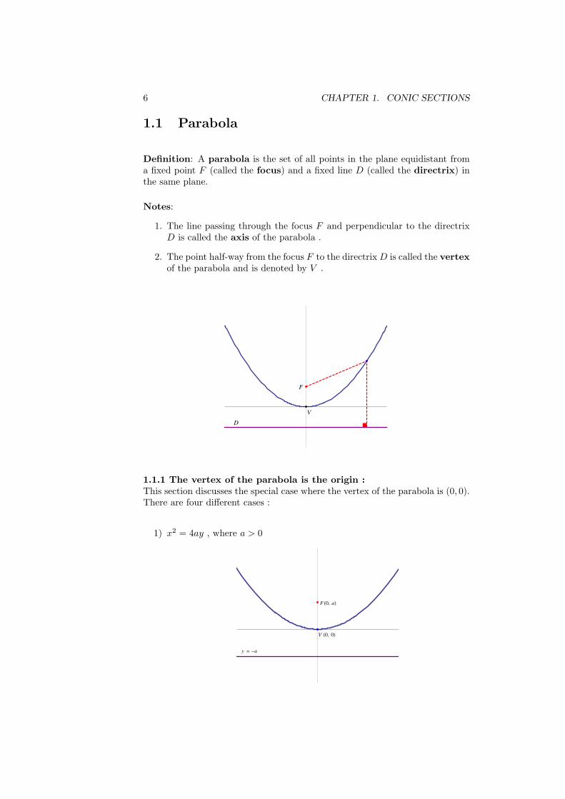
Definition: A parabola is the set of all points in the plane equidistant froma fixed point F (called the focus) and a fixed line D (called the directrix) inthe same plane.
Notes:
1. The line passing through the focus F and perpendicular to the directrixD is called the axis of the parabola .
2. The point half-way from the focus F to the directrixD is called the vertexof the parabola and is denoted by V .
D
V
F
1.1.1 The vertex of the parabola is the origin :This section discusses the special case where the vertex of the parabola is (0, 0).There are four different cases :
1) x2 = 4ay , where a > 0
F H0, aL
V H0, 0L
y = -a
1.1. PARABOLA 7
The parabola opens upwards .
The focus is F (0, a) .
The equation of the directrix is y = −a .
The axis of the parabola is the y-axis .
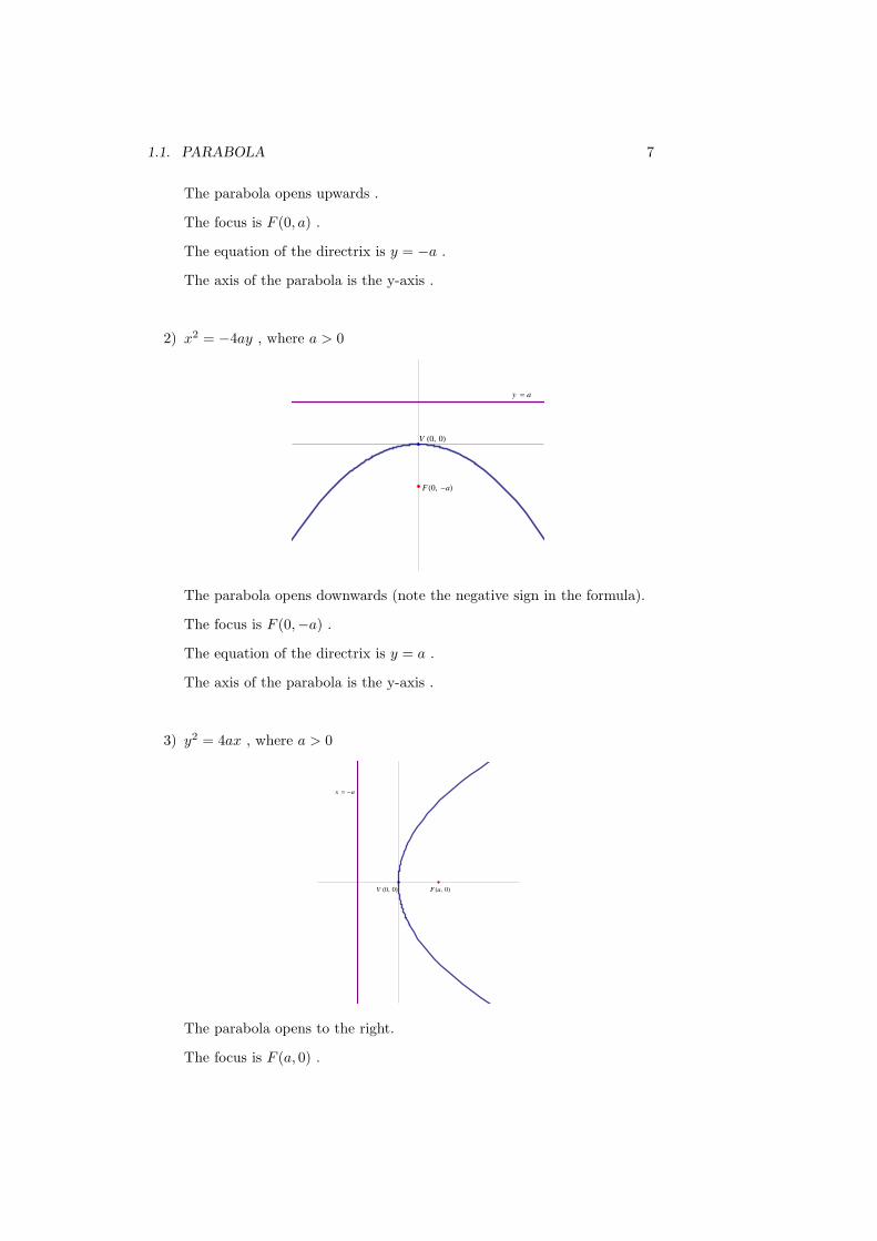
2) x2 = −4ay , where a > 0
F H0, -aL
V H0, 0L
y = a
The parabola opens downwards (note the negative sign in the formula).
The focus is F (0,−a) .
The equation of the directrix is y = a .
The axis of the parabola is the y-axis .
3) y2 = 4ax , where a > 0
F Ha, 0LV H0, 0L
x = -a
The parabola opens to the right.
The focus is F (a, 0) .
8 CHAPTER 1. CONIC SECTIONS
The equation of the directrix is x = −a .
The axis of the parabola is the x-axis .
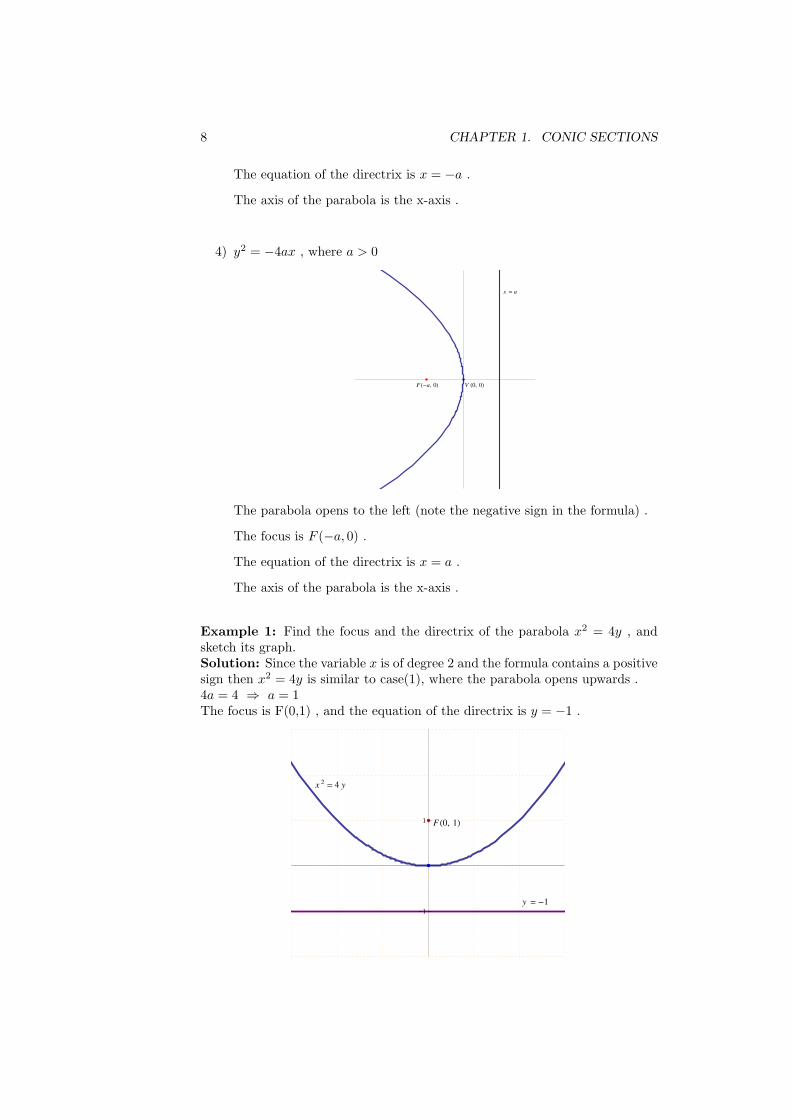
4) y2 = −4ax , where a > 0
x = a
F H-a, 0L V H0, 0L
The parabola opens to the left (note the negative sign in the formula) .
The focus is F (−a, 0) .
The equation of the directrix is x = a .
The axis of the parabola is the x-axis .
Example 1: Find the focus and the directrix of the parabola x2 = 4y , andsketch its graph.Solution: Since the variable x is of degree 2 and the formula contains a positivesign then x2 = 4y is similar to case(1), where the parabola opens upwards .4a = 4 ⇒ a = 1The focus is F(0,1) , and the equation of the directrix is y = −1 .
F H0, 1L
x 2= 4 y
y = -1-1
1

1.1. PARABOLA 9
Example 2: Find the focus and the directrix of the parabola y2 = −8x , andsketch its graph.Solution: Since the variable y is of degree 2 and the formula contains a nega-tive sign then y2 = −8x is similar to case(4), where the parabola opens to theleft .−4a = −8 ⇒ a = 2The focus is F(-2,0) , and the equation of the directrix is x = 2 .
y 2= -8 x
F H-2, 0L
x = 2
-2 2
10 CHAPTER 1. CONIC SECTIONS
1.1.2 The general formula of a parabola :This section discusses the general formula of a parabol where the vertex of theparabola is any point V (h, k) in the plane.There are four different cases :
No. The general formula Focus Directrix The parabola opens1 (x− h)2 = 4a(y − k) F (h, k + a) y = k − a upwards2 (x− h)2 = −4a(y − k) F (h, k − a) y = k + a downwards3 (y − k)2 = 4a(x− h) F (h+ a, k) x = h− a to the right4 (y − k)2 = −4a(x− h) F (h− a, k) x = h+ a to the left
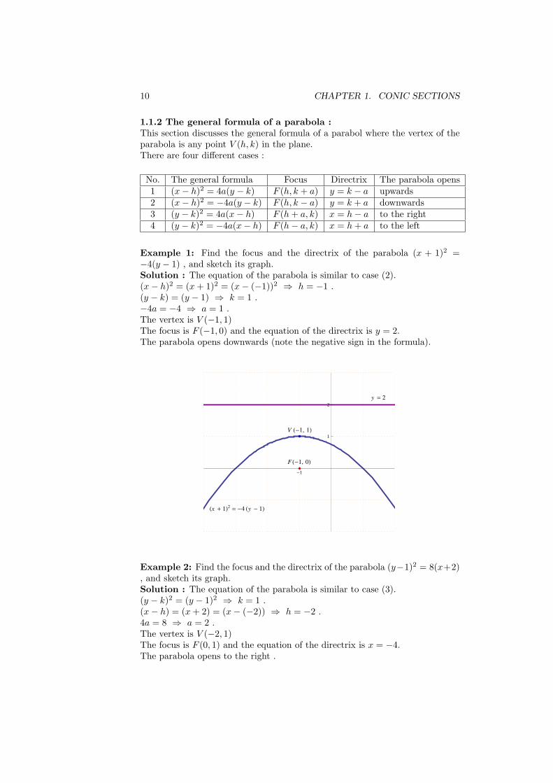
Example 1: Find the focus and the directrix of the parabola (x + 1)2 =−4(y − 1) , and sketch its graph.Solution : The equation of the parabola is similar to case (2).(x− h)2 = (x+ 1)2 = (x− (−1))2 ⇒ h = −1 .(y − k) = (y − 1) ⇒ k = 1 .−4a = −4 ⇒ a = 1 .The vertex is V (−1, 1)The focus is F (−1, 0) and the equation of the directrix is y = 2.The parabola opens downwards (note the negative sign in the formula).
Hx + 1L2 = -4 Hy - 1L
F H-1, 0L
V H-1, 1L
y = 2
-1
1
2
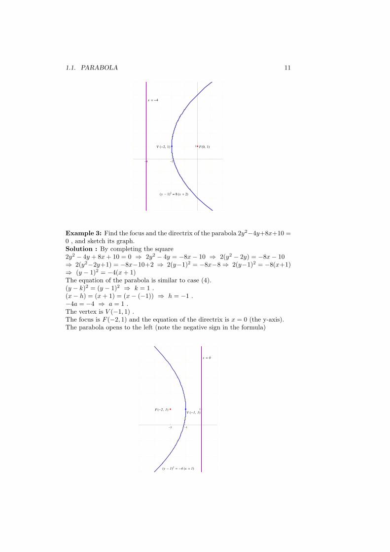
Example 2: Find the focus and the directrix of the parabola (y−1)2 = 8(x+2), and sketch its graph.Solution : The equation of the parabola is similar to case (3).(y − k)2 = (y − 1)2 ⇒ k = 1 .(x− h) = (x+ 2) = (x− (−2)) ⇒ h = −2 .4a = 8 ⇒ a = 2 .The vertex is V (−2, 1)The focus is F (0, 1) and the equation of the directrix is x = −4.The parabola opens to the right .
1.1. PARABOLA 11
Hy - 1L2 = 8 Hx + 2L
F H0, 1LV H-2, 1L
x = -4
-4 -2
1
Example 3: Find the focus and the directrix of the parabola 2y2−4y+8x+10 =0 , and sketch its graph.Solution : By completing the square2y2 − 4y + 8x+ 10 = 0 ⇒ 2y2 − 4y = −8x− 10 ⇒ 2(y2 − 2y) = −8x− 10⇒ 2(y2−2y+1) = −8x−10+2 ⇒ 2(y−1)2 = −8x−8 ⇒ 2(y−1)2 = −8(x+1)⇒ (y − 1)2 = −4(x+ 1)The equation of the parabola is similar to case (4).(y − k)2 = (y − 1)2 ⇒ k = 1 .(x− h) = (x+ 1) = (x− (−1)) ⇒ h = −1 .−4a = −4 ⇒ a = 1 .The vertex is V (−1, 1) .The focus is F (−2, 1) and the equation of the directrix is x = 0 (the y-axis).The parabola opens to the left (note the negative sign in the formula)
F H-2 , 1L
Hy - 1L2 = -4 Hx + 1L
V H-1, 1L
x = 0
-2 -1
1
12 CHAPTER 1. CONIC SECTIONS
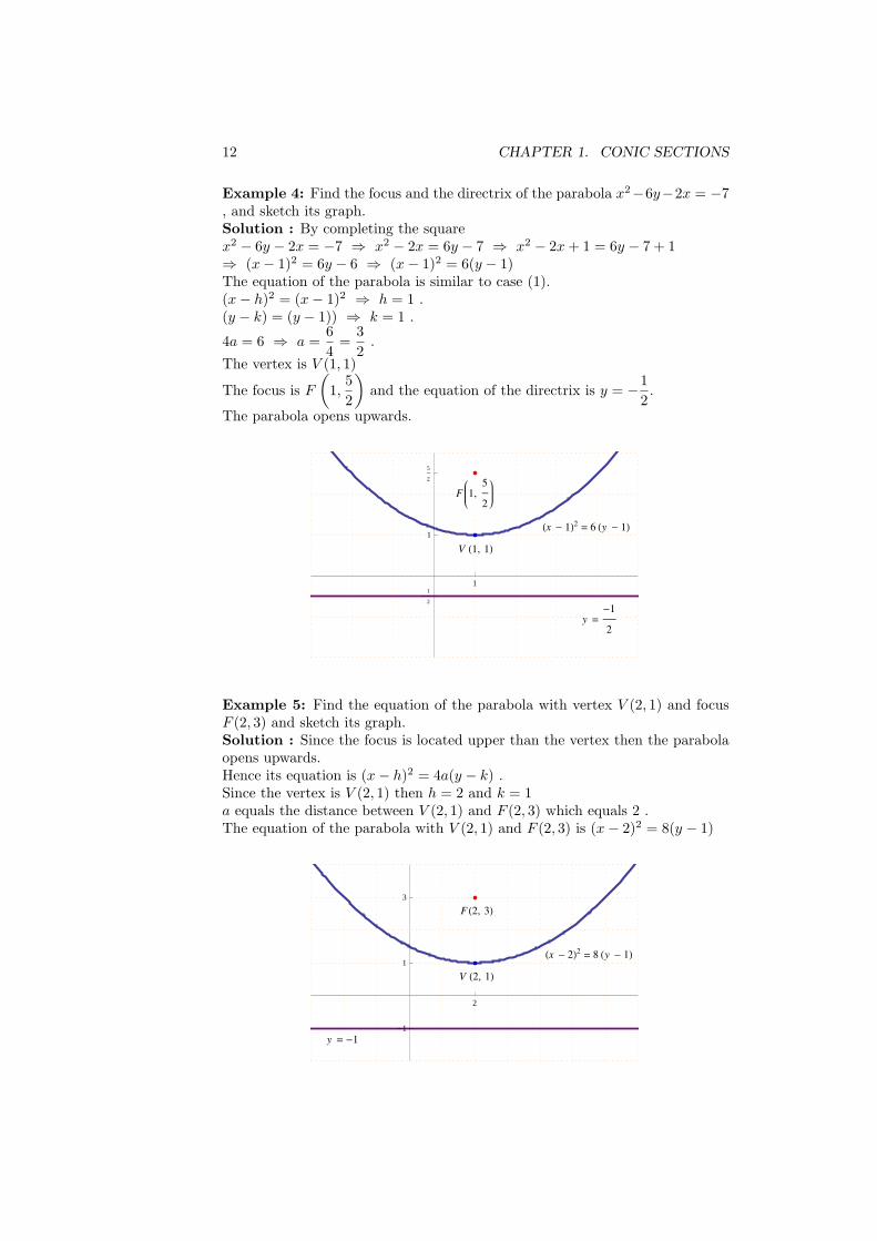
Example 4: Find the focus and the directrix of the parabola x2−6y−2x = −7, and sketch its graph.Solution : By completing the squarex2 − 6y − 2x = −7 ⇒ x2 − 2x = 6y − 7 ⇒ x2 − 2x+ 1 = 6y − 7 + 1⇒ (x− 1)2 = 6y − 6 ⇒ (x− 1)2 = 6(y − 1)The equation of the parabola is similar to case (1).(x− h)2 = (x− 1)2 ⇒ h = 1 .(y − k) = (y − 1)) ⇒ k = 1 .
4a = 6 ⇒ a =6
4=
3
2.
The vertex is V (1, 1)
The focus is F
(
1,5
2
)
and the equation of the directrix is y = −1
2.
The parabola opens upwards.
Hx - 1L2 = 6 Hy - 1L
F 1,5
2
y =-1
2
V H1, 1L
1
-1
2
1
5
2
Example 5: Find the equation of the parabola with vertex V (2, 1) and focusF (2, 3) and sketch its graph.Solution : Since the focus is located upper than the vertex then the parabolaopens upwards.Hence its equation is (x− h)2 = 4a(y − k) .Since the vertex is V (2, 1) then h = 2 and k = 1a equals the distance between V (2, 1) and F (2, 3) which equals 2 .The equation of the parabola with V (2, 1) and F (2, 3) is (x− 2)2 = 8(y − 1)
Hx - 2L2 = 8 Hy - 1L
F H2, 3L
y = -1
V H2, 1L
2
-1
1
3
1.1. PARABOLA 13
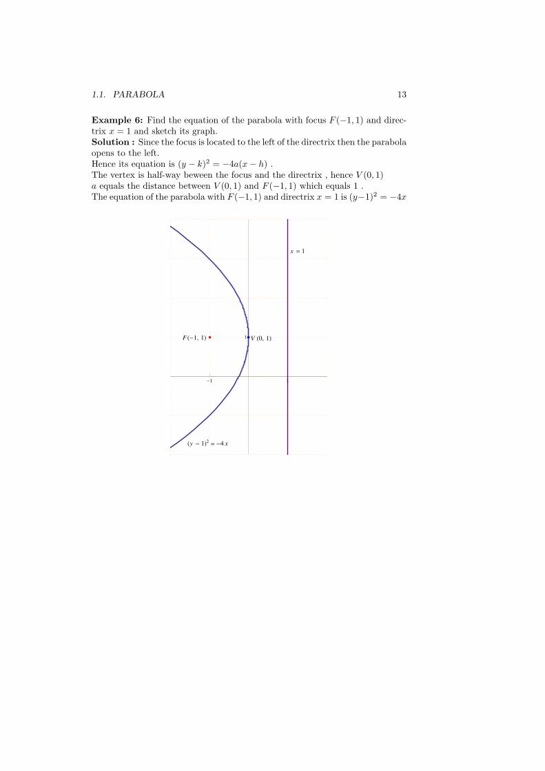
Example 6: Find the equation of the parabola with focus F (−1, 1) and direc-trix x = 1 and sketch its graph.Solution : Since the focus is located to the left of the directrix then the parabolaopens to the left.Hence its equation is (y − k)2 = −4a(x− h) .The vertex is half-way beween the focus and the directrix , hence V (0, 1)a equals the distance between V (0, 1) and F (−1, 1) which equals 1 .The equation of the parabola with F (−1, 1) and directrix x = 1 is (y−1)2 = −4x
Hy - 1L2 = -4 x
F H-1, 1L V H0, 1L
x = 1
-1 1
1
14 CHAPTER 1. CONIC SECTIONS
1.2 Ellipse
Definition: An ellipse is the set of all points in the plane for which the sumof the distances to two fixed points is constant.
Notes :
1. The two fixed points are called the foci of the ellipse and are denoted byF1 and F2.
2. The midpoint between F1 and F2 is called the center of the ellipse andis denoted by P .
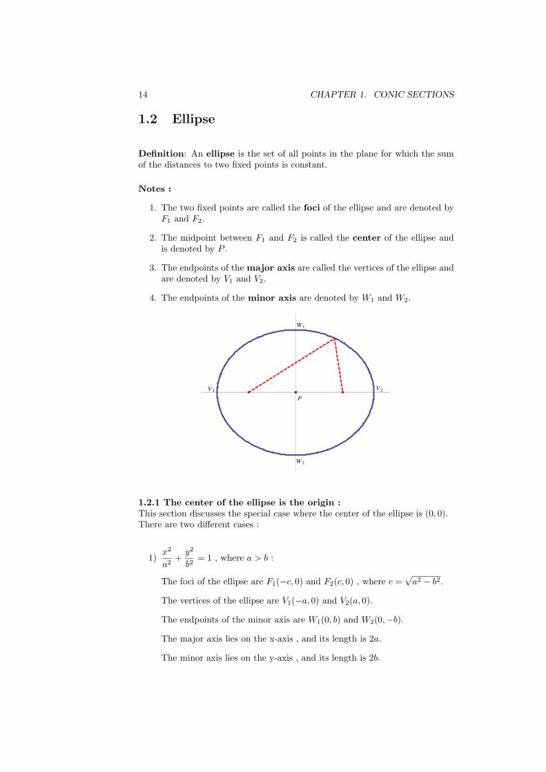
3. The endpoints of the major axis are called the vertices of the ellipse andare denoted by V1 and V2.
4. The endpoints of the minor axis are denoted by W1 and W2.
V 1 V 2
W 1
W 2
P
1.2.1 The center of the ellipse is the origin :This section discusses the special case where the center of the ellipse is (0, 0).There are two different cases :
1)x2
a2+
y2
b2= 1 , where a > b :
The foci of the ellipse are F1(−c, 0) and F2(c, 0) , where c =√a2 − b2.
The vertices of the ellipse are V1(−a, 0) and V2(a, 0).
The endpoints of the minor axis are W1(0, b) and W2(0,−b).
The major axis lies on the x-axis , and its length is 2a.
The minor axis lies on the y-axis , and its length is 2b.
1.2. ELLIPSE 15
F1H-c , 0LV 1H-a, 0L
W 1H0, bL
V 2Ha, 0LF2Hc , 0L
W 2H0, -bL
PH0, 0L
2)x2
a2+
y2
b2= 1 , where b > a :
The foci of the ellipse are F1(0, c) and F2(0,−c) , where c =√b2 − a2.
The vertices of the ellipse are V1(0, b) and V2(0,−b).
The endpoints of the minor axis are W1(−a, 0) and W2(a, 0).
The major axis lies on the y-axis , and its length is 2b.
The minor axis lies on the x-axis , and its length is 2a.
V 1H0, bL
F1H0, cL
W 1H-a, 0L W 2Ha, 0L
F2H0, -cL
V 2H0, -bL
PH0, 0L
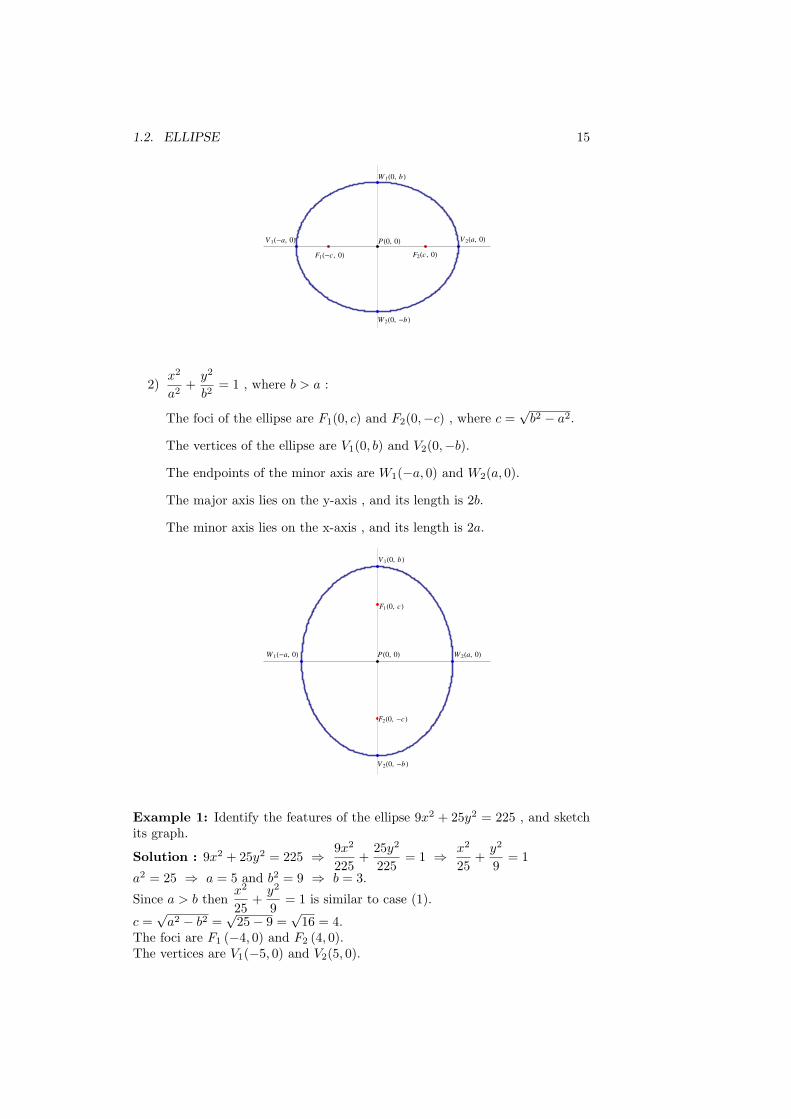
Example 1: Identify the features of the ellipse 9x2 + 25y2 = 225 , and sketchits graph.
Solution : 9x2 + 25y2 = 225 ⇒ 9x2
225+
25y2
225= 1 ⇒ x2
25+
y2
9= 1
a2 = 25 ⇒ a = 5 and b2 = 9 ⇒ b = 3.
Since a > b thenx2
25+
y2
9= 1 is similar to case (1).
c =√a2 − b2 =
√25− 9 =
√16 = 4.
The foci are F1 (−4, 0) and F2 (4, 0).The vertices are V1(−5, 0) and V2(5, 0).
16 CHAPTER 1. CONIC SECTIONS
The endpoints of the minor axis are W1(0, 3) and W2(0,−3).The length of the major axis is 2a = 10.The length of the minor axis is 2b = 6.
V 1H-5, 0L
W 1H0, 3L
F1H-4, 0L F2H4, 0L V 2H5, 0L
W 2H0, -3Lx 2
25+
y 2
9= 1
-5 -4 4 5
-3
3
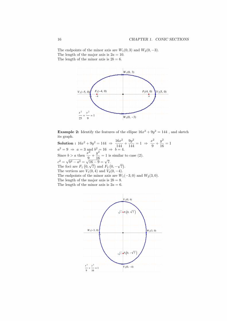
Example 2: Identify the features of the ellipse 16x2 + 9y2 = 144 , and sketchits graph.
Solution : 16x2 + 9y2 = 144 ⇒ 16x2
144+
9y2
144= 1 ⇒ x2
9+
y2
16= 1
a2 = 9 ⇒ a = 3 and b2 = 16 ⇒ b = 4.
Since b > a thenx2
9+
y2
16= 1 is similar to case (2).
c2 =√b2 − a2 =
√16− 9 =
√7.
The foci are F1
(
0,√7)
and F2
(
0,−√7)
.The vertices are V1(0, 4) and V2(0,−4).The endpoints of the minor axis are W1(−3, 0) and W2(3, 0).The length of the major axis is 2b = 8.The length of the minor axis is 2a = 6.
V 2H0, -4L
F2J0, - 7 N
W 2H3, 0LW 1H-3, 0L
V 1H0, 4L
F1J0, 7 N
x 2
9+
y 2
16= 1
-3 3
-4
- 7
7
4
1.2. ELLIPSE 17
1.2.2 The general formula of an ellipse :This section discusses the general formula of an ellipse where the center of theellipse is any point P (h, k) in the plane.There are two different cases :No. The general Formula The Foci The Vertices W1 and W2
1(x− h)2
a2+
(y − k)2
b2= 1 F1(h− c, k) V1(h− a, k) W1(h, k − b)
( a > b ) and c =√a2 − b2 F2(h+ c, k) V2(h+ a, k) W2(h, k + b)
2(x− h)2
a2+
(y − k)2
b2= 1 F1(h, k − c) V1(h, k − b) W1(h− a, k)
( b > a ) and c =√b2 − a2 F2(h, k + c) V2(h, k + b) W2(h+ a, k)
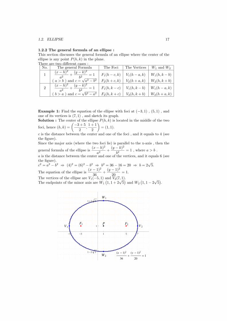
Example 1: Find the equation of the ellipse with foci at (−3, 1) , (5, 1) , andone of its vertices is (7, 1) , and sketch its graph.Solution : The center of the ellipse P (h, k) is located in the middle of the two
foci, hence (h, k) =
(−3 + 5
2,1 + 1
2
)
= (1, 1).
c is the distance between the center and one of the foci , and it equals to 4 (seethe figure).Since the major axis (where the two foci lie) is parallel to the x-axis , then the
general formula of the ellipse is(x− h)2
a2+
(y − k)2
b2= 1 , where a > b .
a is the distance between the center and one of the vertices, and it equals 6 (seethe figure).c2 = a2 − b2 ⇒ (4)2 = (6)2 − b2 ⇒ b2 = 36− 16 = 20 ⇒ b = 2
√5.
The equation of the ellipse is(x− 1)2
36+
(y − 1)2
20= 1.
The vertices of the ellipse are V1(−5, 1) and V2(7, 1).The endpoints of the minor axis are W1
(
1, 1 + 2√5)
and W2
(
1, 1− 2√5)
.
W 2
V 2
F2PF1V 1
W 1
Hx - 1L2
36+
Hy - 1L2
20= 1
-5 -3 1 5 7
1- 2 5
1
1+ 2 5
18 CHAPTER 1. CONIC SECTIONS
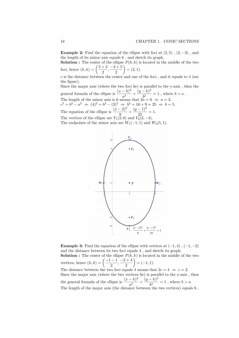
Example 2: Find the equation of the ellipse with foci at (2, 5) , (2,−3) , andthe length of its minor axis equals 6 , and sketch its graph.Solution : The center of the ellipse P (h, k) is located in the middle of the two
foci, hence (h, k) =
(
2 + 2
2,−3 + 5
2
)
= (2, 1).
c is the distance between the center and one of the foci , and it equals to 4 (seethe figure).Since the major axis (where the two foci lie) is parallel to the y-axis , then the
general formula of the ellipse is(x− h)2
a2+
(y − k)2
b2= 1 , where b > a .
The length of the minor axis is 6 means that 2a = 6 ⇒ a = 3.c2 = b2 − a2 ⇒ (4)2 = b2 − (3)2 ⇒ b2 = 16 + 9 = 25 ⇒ b = 5.
The equation of the ellipse is(x− 2)2
9+
(y − 1)2
25= 1.
The vertices of the ellipse are V1(2, 6) and V2(2,−4).The endpoints of the minor axis are W1(−1, 1) and W2(5, 1).
W 2W 1
Hx - 2L2
9+
Hy - 1L2
25= 1
V 1
P
F1
F2
V 2
-1 2 5
-4
-3
1
5
6
Example 3: Find the equation of the ellipse with vertices at (−1, 4) , (−1,−2)and the distance between its two foci equals 4 , and sketch its graph.Solution : The center of the ellipse P (h, k) is located in the middle of the two
vertices, hence (h, k) =
(−1− 1
2,−2 + 4
2
)
= (−1, 1).
The distance between the two foci equals 4 means that 2c = 4 ⇒ c = 2.Since the major axis (where the two vertices lie) is parallel to the y-axis , then
the general formula of the ellipse is(x− h)2
a2+
(y − k)2
b2= 1 , where b > a.
The length of the major axis (the distance between the two vertices) equals 6 ,
1.2. ELLIPSE 19
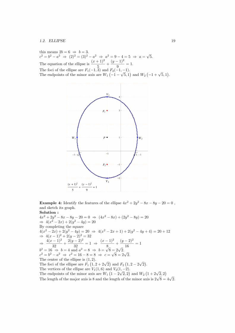
this means 2b = 6 ⇒ b = 3.c2 = b2 − a2 ⇒ (2)2 = (3)2 − a2 ⇒ a2 = 9− 4 = 5 ⇒ a =
√5.
The equation of the ellipse is(x+ 1)2
5+
(y − 1)2
9= 1.
The foci of the ellipse are F1(−1, 3) and F2(−1,−1).The endpoints of the minor axis are W1
(
−1−√5, 1)
and W2
(
−1 +√5, 1)
.
P
V 2
W 2W 1
F1
V 1
Hx + 1L2
5+
Hy - 1L2
9= 1
F2
-1- 5 -1 5 - 1
-2
-1
1
3
4
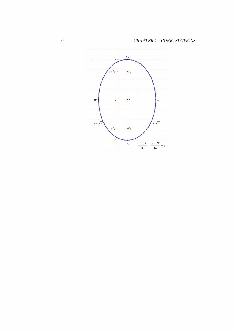
Example 4: Identify the features of the ellipse 4x2 + 2y2 − 8x− 8y − 20 = 0 ,and sketch its graph.Solution :4x2 + 2y2 − 8x− 8y − 20 = 0 ⇒ (4x2 − 8x) + (2y2 − 8y) = 20⇒ 4(x2 − 2x) + 2(y2 − 4y) = 20By completing the square4(x2 − 2x) + 2(y2 − 4y) = 20 ⇒ 4(x2 − 2x+ 1) + 2(y2 − 4y + 4) = 20 + 12⇒ 4(x− 1)2 + 2(y − 2)2 = 32
⇒ 4(x− 1)2
32+
2(y − 2)2
32= 1 ⇒ (x− 1)2
8+
(y − 2)2
16= 1
b2 = 16 ⇒ b = 4 and a2 = 8 ⇒ b =√8 = 2
√2.
c2 = b2 − a2 ⇒ c2 = 16− 8 = 8 ⇒ c =√8 = 2
√2.
The center of the ellipse is (1, 2).The foci of the ellipse are F1
(
1, 2 + 2√2)
and F2
(
1, 2− 2√2)
.The vertices of the ellipse are V1(1, 6) and V2(1,−2).The endpoints of the minor axis are W1
(
1− 2√2, 2)
and W2
(
1 + 2√2, 2)
The length of the major axis is 8 and the length of the minor axis is 2√8 = 4
√2.
20 CHAPTER 1. CONIC SECTIONS
W 2W 1
F1
V 1
F2
V 2Hx - 1L2
8+
Hy - 2L2
16= 1
P
1- 2 2 1 1+ 2 2
-2
2- 2 2
2
2+ 2 2
6
1.3. HYPERBOLA 21
1.3 Hyperbola
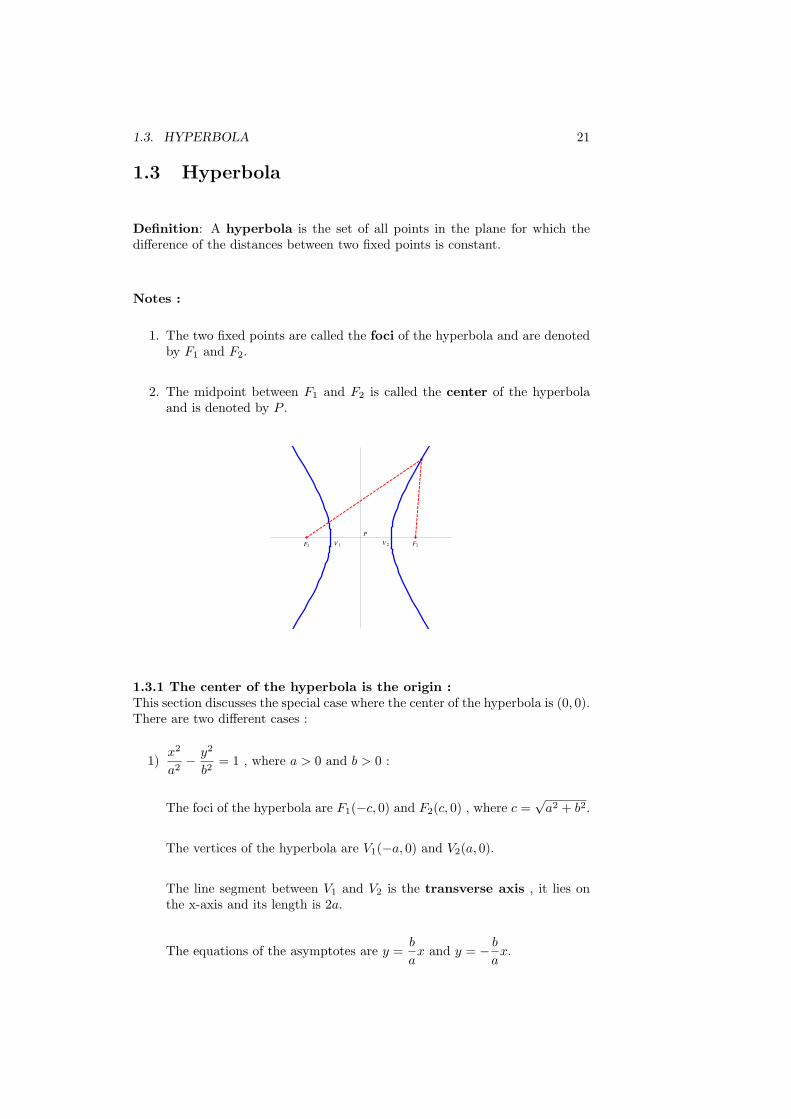
Definition: A hyperbola is the set of all points in the plane for which thedifference of the distances between two fixed points is constant.
Notes :
1. The two fixed points are called the foci of the hyperbola and are denotedby F1 and F2.
2. The midpoint between F1 and F2 is called the center of the hyperbolaand is denoted by P .
V 2F1 V 1 F2
P
1.3.1 The center of the hyperbola is the origin :This section discusses the special case where the center of the hyperbola is (0, 0).There are two different cases :
1)x2
a2− y2
b2= 1 , where a > 0 and b > 0 :
The foci of the hyperbola are F1(−c, 0) and F2(c, 0) , where c =√a2 + b2.
The vertices of the hyperbola are V1(−a, 0) and V2(a, 0).
The line segment between V1 and V2 is the transverse axis , it lies onthe x-axis and its length is 2a.
The equations of the asymptotes are y =b
ax and y = − b
ax.
22 CHAPTER 1. CONIC SECTIONS
F2Hc , 0LF1H-c , 0L
y =-b
ax y =
b
ax
V 1H-a, 0L V 2Ha, 0L
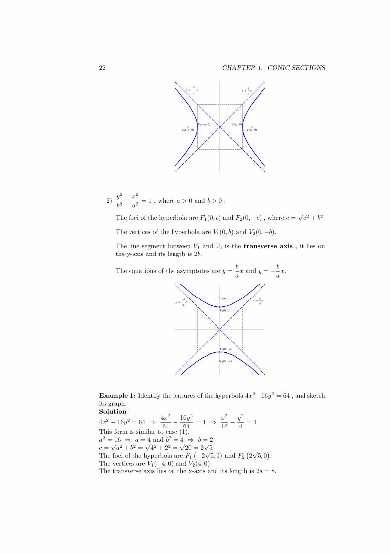
2)y2
b2− x2
a2= 1 , where a > 0 and b > 0 :
The foci of the hyperbola are F1(0, c) and F2(0,−c) , where c =√a2 + b2.
The vertices of the hyperbola are V1(0, b) and V2(0,−b).
The line segment between V1 and V2 is the transverse axis , it lies onthe y-axis and its length is 2b.
The equations of the asymptotes are y =b
ax and y = − b
ax.
F2H0, -cL
V 1H0, bL
F1H0, cLy =-b
ax y =
b
ax
V 2H0, -bL
Example 1: Identify the features of the hyperbola 4x2−16y2 = 64 , and sketchits graph.Solution :
4x2 − 16y2 = 64 ⇒ 4x2
64− 16y2
64= 1 ⇒ x2
16− y2
4= 1
This form is similar to case (1).a2 = 16 ⇒ a = 4 and b2 = 4 ⇒ b = 2c =
√a2 + b2 =
√42 + 22 =
√20 = 2
√5
The foci of the hyperbola are F1
(
−2√5, 0)
and F2
(
2√5, 0)
.The vertices are V1(−4, 0) and V2(4, 0).The transverse axis lies on the x-axis and its length is 2a = 8.
1.3. HYPERBOLA 23
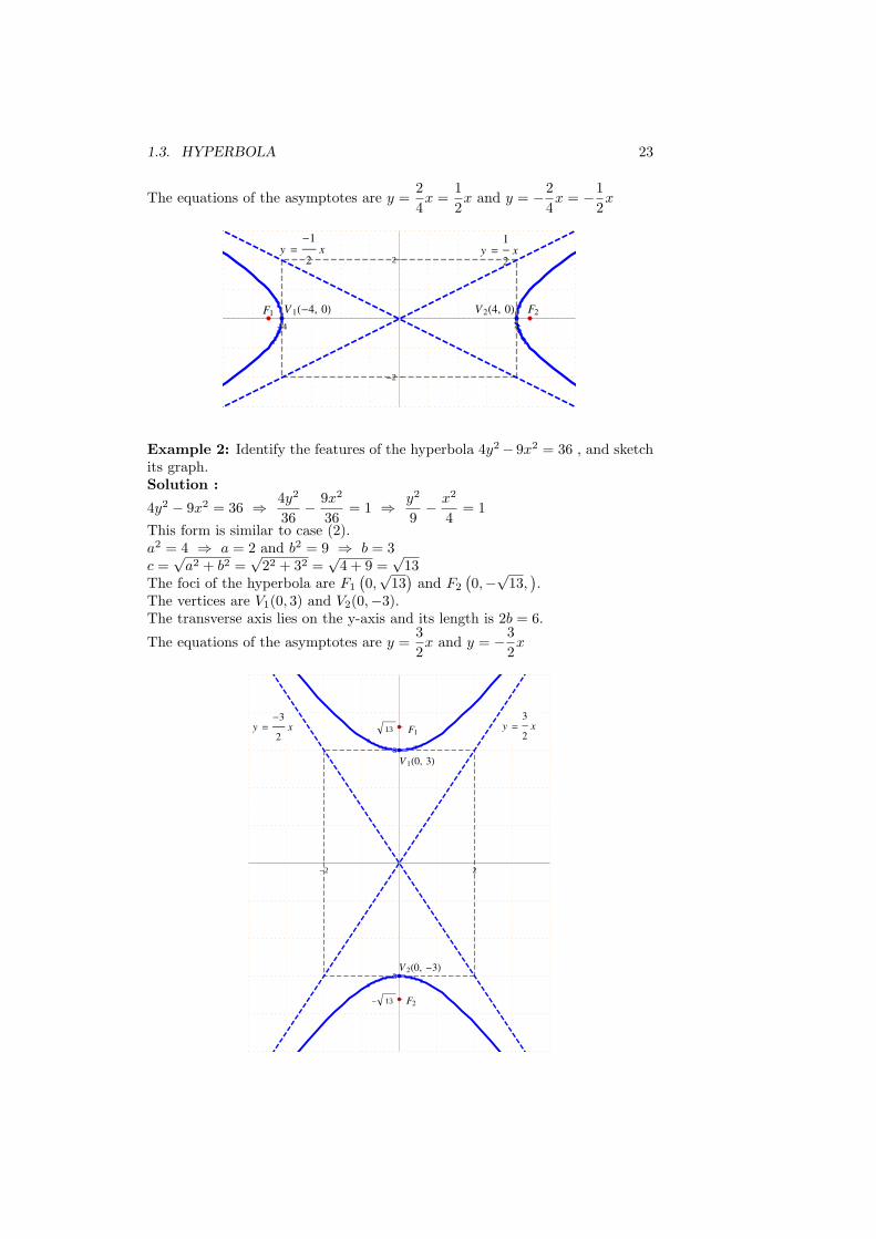
The equations of the asymptotes are y =2
4x =
1
2x and y = −2
4x = −1
2x
F2V 1H-4, 0L V 2H4, 0L
y =1
2xy =
-1
2x
F1
-4 4
-2
2
Example 2: Identify the features of the hyperbola 4y2− 9x2 = 36 , and sketchits graph.Solution :
4y2 − 9x2 = 36 ⇒ 4y2
36− 9x2
36= 1 ⇒ y2
9− x2
4= 1
This form is similar to case (2).a2 = 4 ⇒ a = 2 and b2 = 9 ⇒ b = 3c =
√a2 + b2 =
√22 + 32 =
√4 + 9 =
√13
The foci of the hyperbola are F1
(
0,√13)
and F2
(
0,−√13,)
.The vertices are V1(0, 3) and V2(0,−3).The transverse axis lies on the y-axis and its length is 2b = 6.
The equations of the asymptotes are y =3
2x and y = −3
2x
V 1H0, 3L
y =-3
2x y =
3
2xF1
V 2H0, -3L
F2
-2 2
- 13
-3
3
13
24 CHAPTER 1. CONIC SECTIONS
1.3.2 The general formula of a hyperbola :This section discusses the general formula of a hyperbola where the center ofthe hyperbola is any point P (h, k) in the plane.There are two different cases :No. The general Formula The Foci The Vertices Transverse axis
1(x− h)2
a2− (y − k)2
b2= 1 F1(h− c, k) V1(h− a, k) parallel to
( c2 = a2 + b2 ) F2(h+ c, k) V2(h+ a, k) the x-axis
2(y − k)2
b2− (x− h)2
a2= 1 F1(h, k + c) V1(h, k + b) parallel to
( c2 = a2 + b2 ) F2(h, k − c)) V2(h, k − b) the y-axis
The equations of the asymptotes are y =b
a(x− h) + k and y = − b
a(x− h) + k
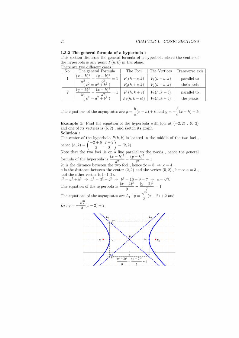
Example 1: Find the equation of the hyperbola with foci at (−2, 2) , (6, 2)and one of its vertices is (5, 2) , and sketch its graph.Solution :The center of the hyperbola P (h, k) is located in the middle of the two foci ,
hence (h, k) =
(−2 + 6
2,2 + 2
2
)
= (2, 2)
Note that the two foci lie on a line parallel to the x-axis , hence the general
formula of the hyperbola is(x− h)2
a2− (y − k)2
b2= 1 .
2c is the distance between the two foci , hence 2c = 8 ⇒ c = 4 .a is the distance between the center (2, 2) and the vertex (5, 2) , hence a = 3 ,and the other vertex is (−1, 2).c2 = a2 + b2 ⇒ 42 = 32 + b2 ⇒ b2 = 16− 9 = 7 ⇒ c =
√7.
The equation of the hyperbola is(x− 2)2
9− (y − 2)2
7= 1
The equations of the asymptotes are L1 : y =
√7
3(x− 2) + 2 and
L2 : y = −√7
3(x− 2) + 2
Hx - 2L2
9-
Hy - 2L2
7= 1
F2V 2
L2 L1
F1 V 1
P
-2 -1 2 5 62- 7
2+ 7
1.3. HYPERBOLA 25
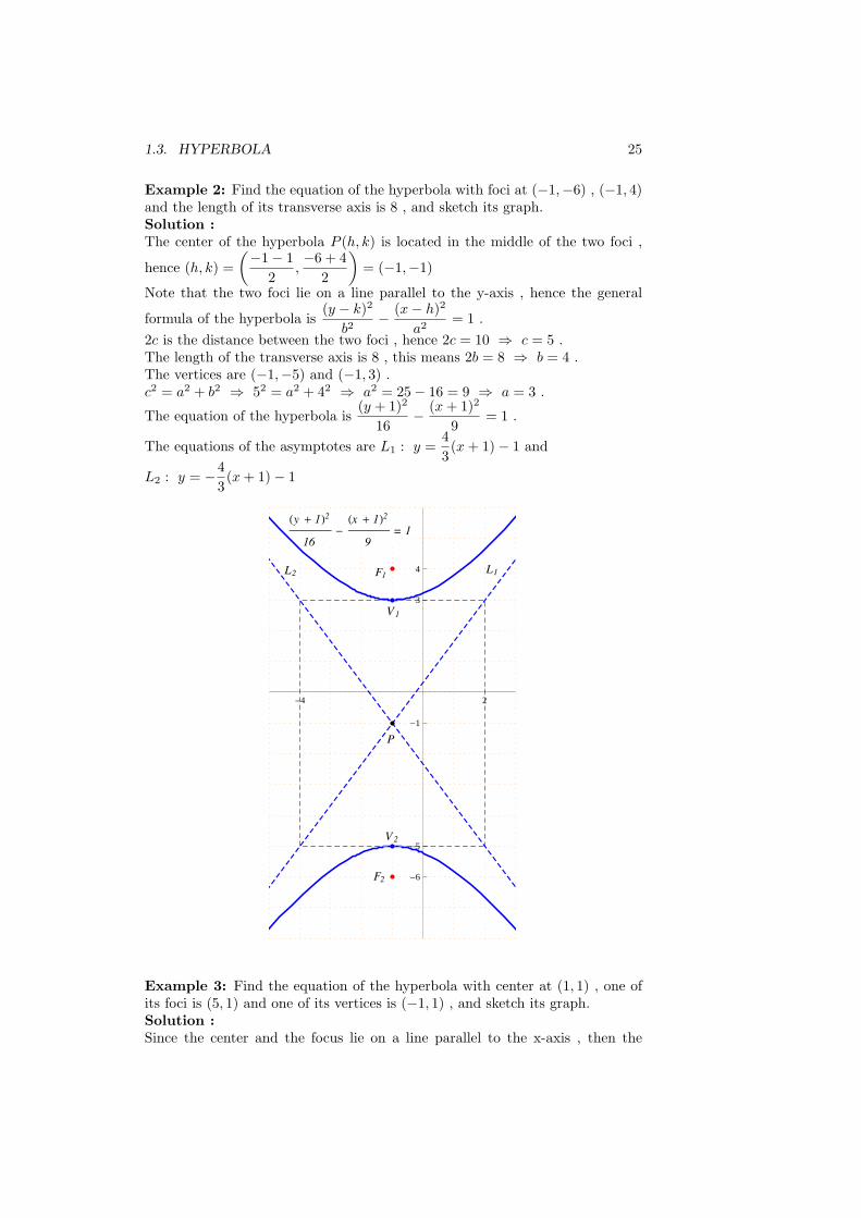
Example 2: Find the equation of the hyperbola with foci at (−1,−6) , (−1, 4)and the length of its transverse axis is 8 , and sketch its graph.Solution :The center of the hyperbola P (h, k) is located in the middle of the two foci ,
hence (h, k) =
(−1− 1
2,−6 + 4
2
)
= (−1,−1)
Note that the two foci lie on a line parallel to the y-axis , hence the general
formula of the hyperbola is(y − k)2
b2− (x− h)2
a2= 1 .
2c is the distance between the two foci , hence 2c = 10 ⇒ c = 5 .The length of the transverse axis is 8 , this means 2b = 8 ⇒ b = 4 .The vertices are (−1,−5) and (−1, 3) .c2 = a2 + b2 ⇒ 52 = a2 + 42 ⇒ a2 = 25− 16 = 9 ⇒ a = 3 .
The equation of the hyperbola is(y + 1)2
16− (x+ 1)2
9= 1 .
The equations of the asymptotes are L1 : y =4
3(x+ 1)− 1 and
L2 : y = −4
3(x+ 1)− 1
P
F2
L2
V 1
F1
Hy + 1L2
16-
Hx + 1L2
9= 1
L1
V 2
-4 2
-6
-5
-1
3
4
Example 3: Find the equation of the hyperbola with center at (1, 1) , one ofits foci is (5, 1) and one of its vertices is (−1, 1) , and sketch its graph.Solution :Since the center and the focus lie on a line parallel to the x-axis , then the
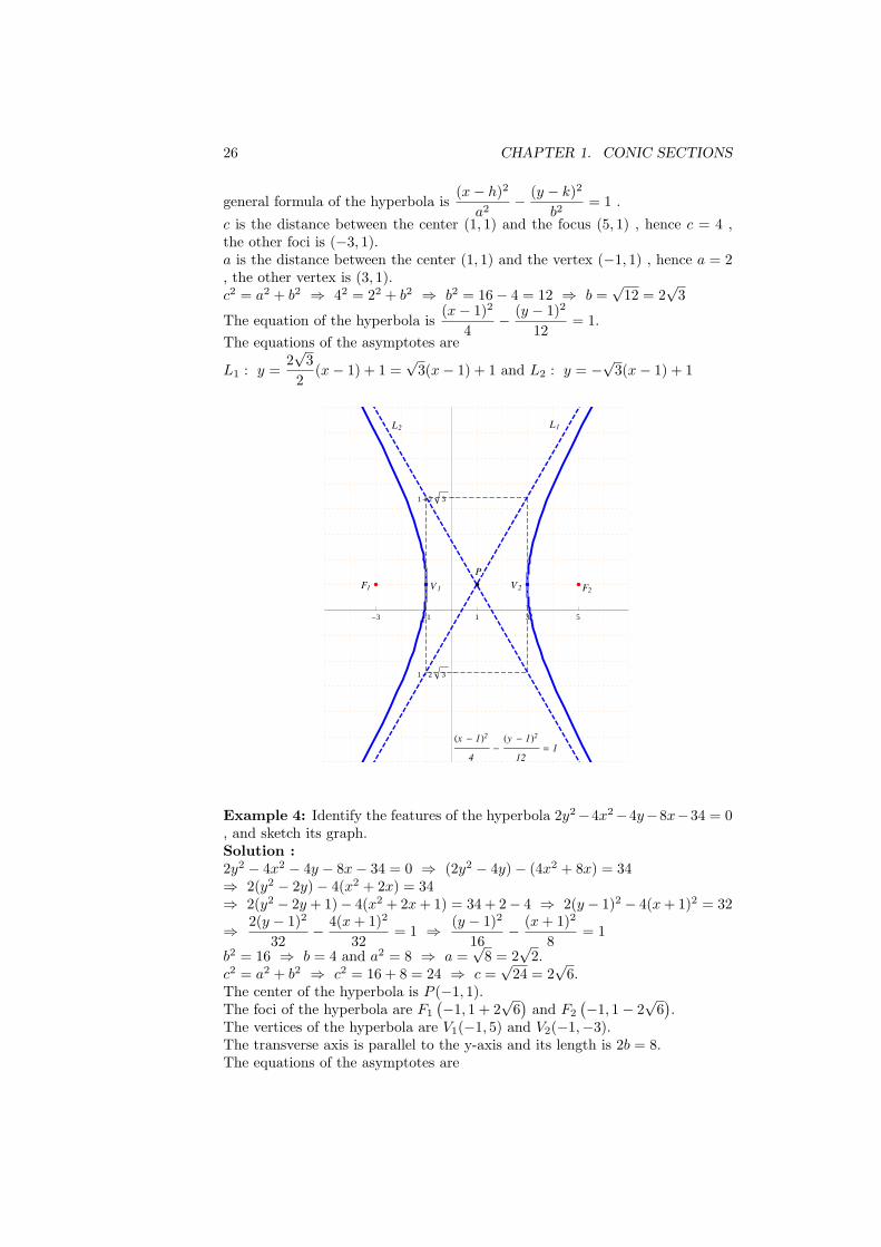
26 CHAPTER 1. CONIC SECTIONS
general formula of the hyperbola is(x− h)2
a2− (y − k)2
b2= 1 .
c is the distance between the center (1, 1) and the focus (5, 1) , hence c = 4 ,the other foci is (−3, 1).a is the distance between the center (1, 1) and the vertex (−1, 1) , hence a = 2, the other vertex is (3, 1).c2 = a2 + b2 ⇒ 42 = 22 + b2 ⇒ b2 = 16− 4 = 12 ⇒ b =
√12 = 2
√3
The equation of the hyperbola is(x− 1)2
4− (y − 1)2
12= 1.
The equations of the asymptotes are
L1 : y =2√3
2(x− 1) + 1 =
√3(x− 1) + 1 and L2 : y = −
√3(x− 1) + 1
Hx - 1L2
4-
Hy - 1L2
12= 1
V 2F1
L2 L1
V 1 F2
P
-3 -1 1 3 5
1- 2 3
1+ 2 3
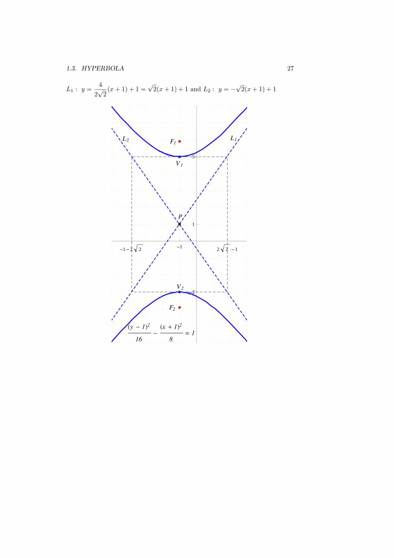
Example 4: Identify the features of the hyperbola 2y2−4x2−4y−8x−34 = 0, and sketch its graph.Solution :2y2 − 4x2 − 4y − 8x− 34 = 0 ⇒ (2y2 − 4y)− (4x2 + 8x) = 34⇒ 2(y2 − 2y)− 4(x2 + 2x) = 34⇒ 2(y2 − 2y + 1)− 4(x2 + 2x+ 1) = 34 + 2− 4 ⇒ 2(y − 1)2 − 4(x+ 1)2 = 32
⇒ 2(y − 1)2
32− 4(x+ 1)2
32= 1 ⇒ (y − 1)2
16− (x+ 1)2
8= 1
b2 = 16 ⇒ b = 4 and a2 = 8 ⇒ a =√8 = 2
√2.
c2 = a2 + b2 ⇒ c2 = 16 + 8 = 24 ⇒ c =√24 = 2
√6.
The center of the hyperbola is P (−1, 1).The foci of the hyperbola are F1
(
−1, 1 + 2√6)
and F2
(
−1, 1− 2√6)
.The vertices of the hyperbola are V1(−1, 5) and V2(−1,−3).The transverse axis is parallel to the y-axis and its length is 2b = 8.The equations of the asymptotes are
1.3. HYPERBOLA 27
L1 : y =4
2√2(x+ 1) + 1 =
√2(x+ 1) + 1 and L2 : y = −
√2(x+ 1) + 1
Hy - 1L2
16-
Hx + 1L2
8= 1
F2
L1L2 F1
V 1
V 2
P
-1- 2 2 -1 2 2 - 1
-3
1
5

28 CHAPTER 1. CONIC SECTIONS
Chapter 2
MATRICES ANDDETERMINANTS
2.1 Matrices
2.2 Determinants
29
30 CHAPTER 2. MATRICES AND DETERMINANTS
2.1 Matrices
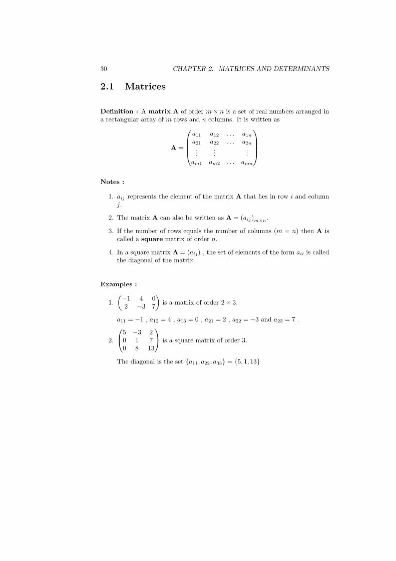
Definition : A matrix A of order m× n is a set of real numbers arranged ina rectangular array of m rows and n columns. It is written as
A =
a11 a12 . . . a1na21 a22 . . . a2n...
......
am1 am2 . . . amn
Notes :
1. aij represents the element of the matrix A that lies in row i and columnj.
2. The matrix A can also be written as A = (aij)m×n.
3. If the number of rows equals the number of columns (m = n) then A iscalled a square matrix of order n.
4. In a square matrix A = (aij) , the set of elements of the form aii is calledthe diagonal of the matrix.
Examples :
1.
(
−1 4 02 −3 7
)
is a matrix of order 2× 3.
a11 = −1 , a12 = 4 , a13 = 0 , a21 = 2 , a22 = −3 and a23 = 7 .
2.
5 −3 20 1 70 8 13
is a square matrix of order 3.
The diagonal is the set {a11, a22, a33} = {5, 1, 13}
2.1. MATRICES 31
2.1.1 Special types of matrices :
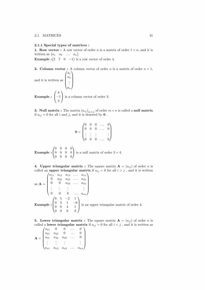
1. Row vector : A row vector of order n is a matrix of order 1× n, and it iswritten as
(
a1 a2 . . . an)
Example :(
2 7 0 −1)
is a row vector of order 4.
2. Column vector : A column vector of order n is a matrix of order n × 1,
and it is written as
a1a2...an
Example :
8−12
is a column vector of order 3.
3. Null matrix : The matrix (aij)m×n of order m×n is called a null matrixif aij = 0 for all i and j, and it is denoted by 0 .
0 =
0 0 0 . . . 00 0 0 . . . 0...
......
...0 0 0 . . . 0
Example :
0 0 0 00 0 0 00 0 0 0
is a null matrix of order 3× 4.
4. Upper triangular matrix : The square matrix A = (aij) of order n iscalled an upper triangular matrix if aij = 0 for all i > j , and it is written
as A =
a11 a12 a13 . . . a1n0 a22 a23 . . . a2n0 0 a33 . . . a3n...
......
...0 0 0 . . . ann
Example :
8 5 −2 10 3 1 −60 0 4 10 0 0 3
is an upper triangular matrix of order 4.
5. Lower triangular matrix : The square matrix A = (aij) of order n iscalled a lower triangular matrix if aij = 0 for all i < j , and it is written as
A =
a11 0 0 . . . 0a21 a22 0 . . . 0a31 a32 a33 . . . 0...
......
...an1 an2 an3 . . . ann
32 CHAPTER 2. MATRICES AND DETERMINANTS
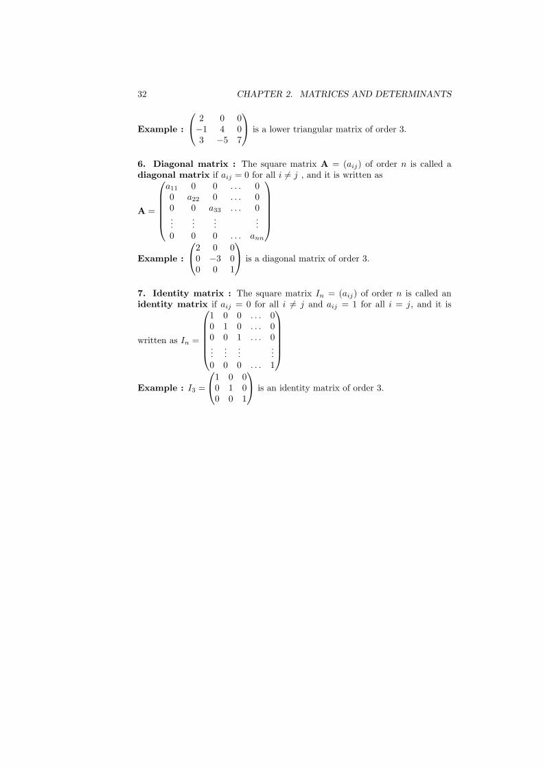
Example :
2 0 0−1 4 03 −5 7
is a lower triangular matrix of order 3.
6. Diagonal matrix : The square matrix A = (aij) of order n is called adiagonal matrix if aij = 0 for all i 6= j , and it is written as
A =
a11 0 0 . . . 00 a22 0 . . . 00 0 a33 . . . 0...
......
...0 0 0 . . . ann
Example :
2 0 00 −3 00 0 1
is a diagonal matrix of order 3.
7. Identity matrix : The square matrix In = (aij) of order n is called anidentity matrix if aij = 0 for all i 6= j and aij = 1 for all i = j, and it is
written as In =
1 0 0 . . . 00 1 0 . . . 00 0 1 . . . 0...
......
...0 0 0 . . . 1
Example : I3 =
1 0 00 1 00 0 1
is an identity matrix of order 3.
2.1. MATRICES 33
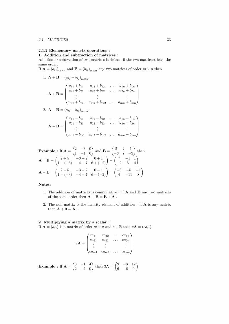
2.1.2 Elementary matrix operations :1. Addition and subtraction of matrices :Addition or subtraction of two matrices is defined if the two matricest have thesame order.If A = (aij)m×n and B = (bij)m×n any two matrices of order m× n then
1. A+B = (aij + bij)m×n.
A+B =
a11 + b11 a12 + b12 . . . a1n + b1na21 + b21 a22 + b22 . . . a2n + b2n
......
...am1 + bm1 am2 + bm2 . . . amn + bmn
2. A−B = (aij − bij)m×n.
A−B =
a11 − b11 a12 − b12 . . . a1n − b1na21 − b21 a22 − b22 . . . a2n − b2n
......
...am1 − bm1 am2 − bm2 . . . amn − bmn
Example : If A =
(
2 −3 01 −4 6
)
and B =
(
5 2 1−3 7 −2
)
then
A+B =
(
2 + 5 −3 + 2 0 + 11 + (−3) −4 + 7 6 + (−2)
)
=
(
7 −1 1−2 3 4
)
A−B =
(
2− 5 −3− 2 0− 11− (−3) −4− 7 6− (−2)
)
=
(
−3 −5 −14 −11 8
)
Notes:
1. The addition of matrices is commutative : if A and B any two matricesof the same order then A+B = B+A .
2. The null matrix is the identity element of addition : if A is any matrixthen A+ 0 = A .
2. Multiplying a matrix by a scalar :If A = (aij) is a matrix of order m× n and c ∈ R then cA = (caij).
cA =
ca11 ca12 . . . ca1nca21 ca22 . . . ca2n...
......
cam1 cam2 . . . camn
Example : If A =
(
3 −1 42 −2 0
)
then 3A =
(
9 −3 126 −6 0
)
34 CHAPTER 2. MATRICES AND DETERMINANTS
3. Multiplying a row vector by a column vector :If A =
(
a1 a2 . . . an)
is a row vector of order n and
B =
b1b2...bn
is a column vector of order n then
AB =(
a1 a2 . . . an)
b1b2...bn
= a1b1 + a2b2 + . . .+ anbn
Example : If A =(
−1 2 0 5)
and B =
4−21−1
then
AB =(
−1 2 0 5)
4−21−1
= −4− 4 + 0− 5 = −13
4. Multiplication of matrices :
1. If A and B any two matrices then AB is defined if the number of columnsof A equals the number of rows of B .
2. If A = (aij)m×n and B = (bij)n×p then AB = (cij)m×p.
cij is calculated by multiplying the ith row of A by the jth column of B.
cij =(
ai1 ai2 . . . ain)
b1jb2j...
bnj
= ai1b1j + ai2b2j + . . .+ ainbnj
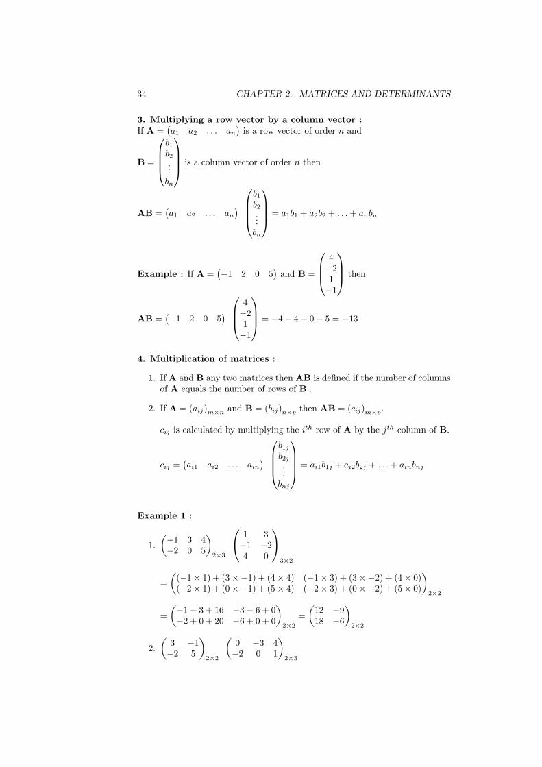
Example 1 :
1.
(
−1 3 4−2 0 5
)
2×3
1 3−1 −24 0
3×2
=
(
(−1× 1) + (3×−1) + (4× 4) (−1× 3) + (3×−2) + (4× 0)(−2× 1) + (0×−1) + (5× 4) (−2× 3) + (0×−2) + (5× 0)
)
2×2
=
(
−1− 3 + 16 −3− 6 + 0−2 + 0 + 20 −6 + 0 + 0
)
2×2
=
(
12 −918 −6
)
2×2
2.
(
3 −1−2 5
)
2×2
(
0 −3 4−2 0 1
)
2×3
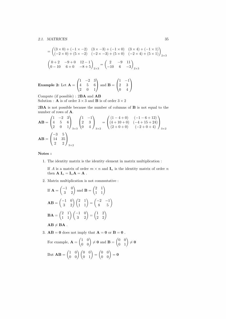
2.1. MATRICES 35
=
(
(3× 0) + (−1×−2) (3×−3) + (−1× 0) (3× 4) + (−1× 1)(−2× 0) + (5×−2) (−2×−3) + (5× 0) (−2× 4) + (5× 1)
)
2×3
(
0 + 2 −9 + 0 12− 10− 10 6 + 0 −8 + 5
)
2×3
=
(
2 −9 11−10 6 −3
)
2×3
Example 2: Let A =
1 −2 34 5 62 0 1
and B =
1 −12 30 4
Compute (if possible) : 2BA and ABSolution : A is of order 3× 3 and B is of order 3× 2
2BA is not possible because the number of columns of B is not equal to thenumber of rows of A.
AB =
1 −2 34 5 62 0 1
3×3
1 −12 30 4
3×2
=
(1− 4 + 0) (−1− 6 + 12)(4 + 10 + 0) (−4 + 15 + 24)(2 + 0 + 0) (−2 + 0 + 4)
3×2
AB =
−3 514 352 2
3×2
Notes :
1. The identity matrix is the identity element in matrix multiplication :
If A is a matrix of order m × n and In is the identity matrix of order n
then A In = InA = A .
2. Matrix multiplication is not commutative :
If A =
(
−1 03 2
)
and B =
(
2 11 1
)
AB =
(
−1 03 2
)(
2 11 1
)
=
(
−2 −18 5
)
BA =
(
2 11 1
)(
−1 03 2
)
=
(
1 22 2
)
AB 6= BA .
3. AB = 0 does not imply that A = 0 or B = 0 .
For example, A =
(
1 00 0
)
6= 0 and B =
(
0 00 1
)
6= 0
But AB =
(
1 00 0
)(
0 00 1
)
=
(
0 00 0
)
= 0
36 CHAPTER 2. MATRICES AND DETERMINANTS
2.1.3 Transpose of a matrix :If A = (aij)m×n then the transpose of A is At = (aji)n×m.
Example : If A =
(
4 0 −2−3 5 1
)
then At =
4 −30 5−2 1
Note : The transpose of a lower triangular matrix is an upper triangular matrix, and the transpose of an upper triangular matrix is a lower triangular matrix .
Theorem :If A and B any two matrices and λ ∈ R then
1.(
At)t
= A .
2. (A+B)t= At +Bt .
3. (λA)t= λ At .
4. (AB)t= BtAt .
2.1.4 Properties of operations on matrices :
1. If A , B and C any three matrices of the same order then
A+B+C = (A+B) +C = A+ (B+C) = (A+C) +B
2. If A , B any two matrices of order m× n and C a matrix of order n× p
then (A+B)C = AC+BC
3. If A , B any two matrices of order m× n and C a matrix of order p×m
then C(A+B) = CA+CB
4. If A a matrix of order m× n , B a matrix of order n× p and C a matrixof order p× q then ABC = (AB)C = A(BC)
2.2. DETERMINANTS 37
2.2 Determinants
If A is a square matrix then the determinant of A is denoted by det(A) or |A|.
2.2.1 The determinant of a 2× 2 matrix :
If A =
(
a11 a12a21 a22
)
then |A| =∣
∣
∣
∣
a11 a12a21 a22
∣
∣
∣
∣
= a11a22 − a12a21
Example :
If A =
(
5 −12 3
)
then |A| = (5× 3)− (2×−1) = 15 + 2 = 17
2.2.2 The determinant of a 3× 3 matrix :
Let A =
a11 a12 a13a21 a22 a23a31 a32 a33
be a square matrix of order 3.
1). The determinant of A is defined as :
|A| = a11
∣
∣
∣
∣
a22 a23a32 a33
∣
∣
∣
∣
− a12
∣
∣
∣
∣
a21 a23a31 a33
∣
∣
∣
∣
+ a13
∣
∣
∣
∣
a21 a22a31 a32
∣
∣
∣
∣
|A| = a11 (a22a33 − a23a32)− a12 (a21a33 − a23a31) + a13 (a21a32 − a22a31)
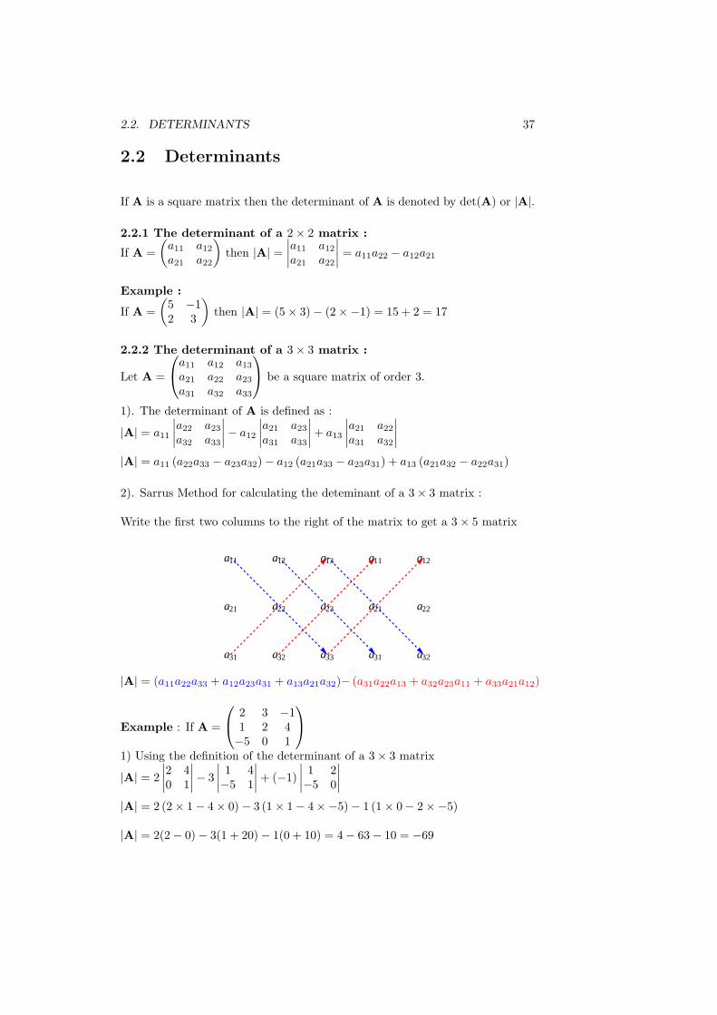
2). Sarrus Method for calculating the deteminant of a 3× 3 matrix :
Write the first two columns to the right of the matrix to get a 3× 5 matrix
a11 a12 a13 a11 a12
a21 a22 a23 a21 a22
a31 a32 a33 a31 a32
|A| = (a11a22a33 + a12a23a31 + a13a21a32)− (a31a22a13 + a32a23a11 + a33a21a12)
Example : If A =
2 3 −11 2 4−5 0 1
1) Using the definition of the determinant of a 3× 3 matrix
|A| = 2
∣
∣
∣
∣
2 40 1
∣
∣
∣
∣
− 3
∣
∣
∣
∣
1 4−5 1
∣
∣
∣
∣
+ (−1)
∣
∣
∣
∣
1 2−5 0
∣
∣
∣
∣
|A| = 2 (2× 1− 4× 0)− 3 (1× 1− 4×−5)− 1 (1× 0− 2×−5)
|A| = 2(2− 0)− 3(1 + 20)− 1(0 + 10) = 4− 63− 10 = −69
38 CHAPTER 2. MATRICES AND DETERMINANTS
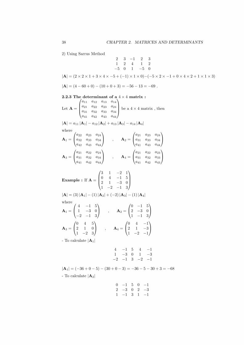
2) Using Sarrus Method2 3 −1 2 31 2 4 1 2−5 0 1 −5 0
|A| = (2× 2× 1 + 3× 4×−5 + (−1)× 1× 0)−(−5× 2×−1 + 0× 4× 2 + 1× 1× 3)
|A| = (4− 60 + 0)− (10 + 0 + 3) = −56− 13 = −69 .
2.2.3 The determinant of a 4× 4 matrix :
Let A =
a11 a12 a13 a14a21 a22 a23 a24a31 a32 a33 a34a41 a42 a43 a44
be a 4× 4 matrix , then
|A| = a11 |A1| − a12 |A2|+ a13 |A3| − a14 |A4|where
A1 =
a22 a23 a24a32 a33 a34a42 a43 a44
, A2 =
a21 a23 a24a31 a33 a34a41 a43 a44
A3 =
a21 a22 a24a31 a32 a34a41 a42 a44
, A4 =
a21 a22 a23a31 a32 a33a41 a42 a43
Example : If A =
3 1 −2 10 4 −1 52 1 −3 01 −2 −1 3
|A| = (3) |A1| − (1) |A2|+ (−2) |A3| − (1) |A4|where
A1 =
4 −1 51 −3 0−2 −1 3
, A2 =
0 −1 52 −3 01 −1 3
A3 =
0 4 52 1 01 −2 3
, A4 =
0 4 −12 1 −31 −2 −1
- To calculate |A1|
4 −1 5 4 −11 −3 0 1 −3−2 −1 3 −2 −1
|A1| = (−36 + 0− 5)− (30 + 0− 3) = −36− 5− 30 + 3 = −68
- To calculate |A2|
0 −1 5 0 −12 −3 0 2 −31 −1 3 1 −1
2.2. DETERMINANTS 39
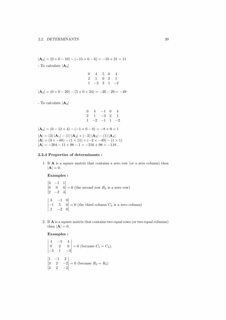
|A2| = (0 + 0− 10)− (−15 + 0− 6) = −10 + 21 = 11
- To calculate |A3|
0 4 5 0 42 1 0 2 11 −2 3 1 −2
|A3| = (0 + 0− 20)− (5 + 0 + 24) = −20− 29 = −49
- To calculate |A4|
0 4 −1 0 42 1 −3 2 11 −2 −1 1 −2
|A4| = (0− 12 + 4)− (−1 + 0− 8) = −8 + 9 = 1
|A| = (3) |A1| − (1) |A2|+ (−2) |A3| − (1) |A4||A| = (3×−68)− (1× 11) + (−2×−49)− (1× 1)|A| = −204− 11 + 98− 1 = −216 + 98 = −118 .
2.2.4 Properties of determinants :
1. If A is a square matrix that contains a zero row (or a zero column) then|A| = 0.
Examples :∣
∣
∣
∣
∣
∣
3 −1 10 0 02 −2 4
∣
∣
∣
∣
∣
∣
= 0 (the second row R2 is a zero row)
∣
∣
∣
∣
∣
∣
3 −1 0−1 5 02 −2 0
∣
∣
∣
∣
∣
∣
= 0 (the third column C3 is a zero column)
2. IfA is a square matrix that contains two equal rows (or two equal columns)then |A| = 0.
Examples :∣
∣
∣
∣
∣
∣
4 −5 40 2 0−3 1 −3
∣
∣
∣
∣
∣
∣
= 0 (because C1 = C3).
∣
∣
∣
∣
∣
∣
1 −1 23 2 −23 2 −2
∣
∣
∣
∣
∣
∣
= 0 (because R2 = R3)
40 CHAPTER 2. MATRICES AND DETERMINANTS
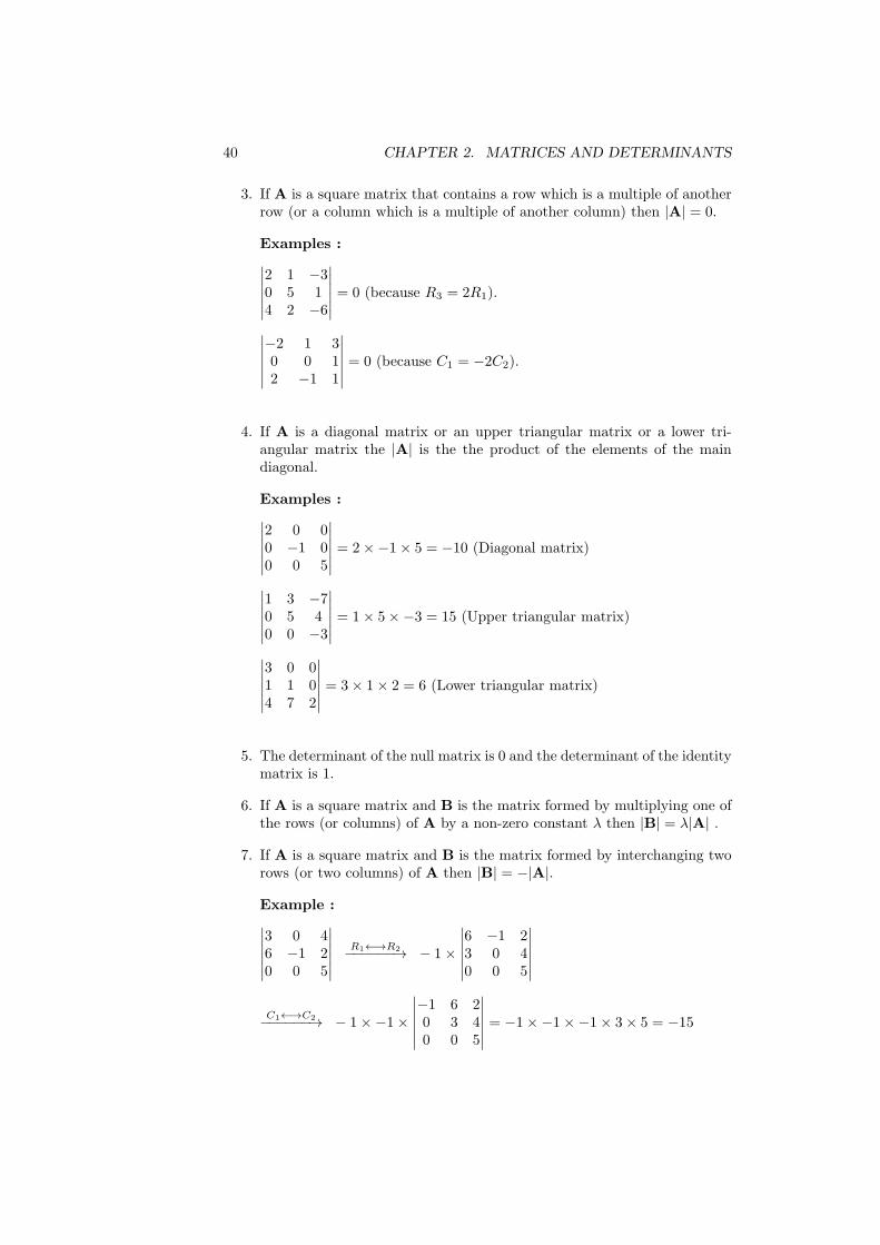
3. If A is a square matrix that contains a row which is a multiple of anotherrow (or a column which is a multiple of another column) then |A| = 0.
Examples :
∣
∣
∣
∣
∣
∣
2 1 −30 5 14 2 −6
∣
∣
∣
∣
∣
∣
= 0 (because R3 = 2R1).
∣
∣
∣
∣
∣
∣
−2 1 30 0 12 −1 1
∣
∣
∣
∣
∣
∣
= 0 (because C1 = −2C2).
4. If A is a diagonal matrix or an upper triangular matrix or a lower tri-angular matrix the |A| is the the product of the elements of the maindiagonal.
Examples :
∣
∣
∣
∣
∣
∣
2 0 00 −1 00 0 5
∣
∣
∣
∣
∣
∣
= 2×−1× 5 = −10 (Diagonal matrix)
∣
∣
∣
∣
∣
∣
1 3 −70 5 40 0 −3
∣
∣
∣
∣
∣
∣
= 1× 5×−3 = 15 (Upper triangular matrix)
∣
∣
∣
∣
∣
∣
3 0 01 1 04 7 2
∣
∣
∣
∣
∣
∣
= 3× 1× 2 = 6 (Lower triangular matrix)
5. The determinant of the null matrix is 0 and the determinant of the identitymatrix is 1.
6. If A is a square matrix and B is the matrix formed by multiplying one ofthe rows (or columns) of A by a non-zero constant λ then |B| = λ|A| .
7. If A is a square matrix and B is the matrix formed by interchanging tworows (or two columns) of A then |B| = −|A|.
Example :
∣
∣
∣
∣
∣
∣
3 0 46 −1 20 0 5
∣
∣
∣
∣
∣
∣
R1←→R2−−−−−−→ − 1×
∣
∣
∣
∣
∣
∣
6 −1 23 0 40 0 5
∣
∣
∣
∣
∣
∣
C1←→C2−−−−−−→ − 1×−1×
∣
∣
∣
∣
∣
∣
−1 6 20 3 40 0 5
∣
∣
∣
∣
∣
∣
= −1×−1×−1× 3× 5 = −15
2.2. DETERMINANTS 41
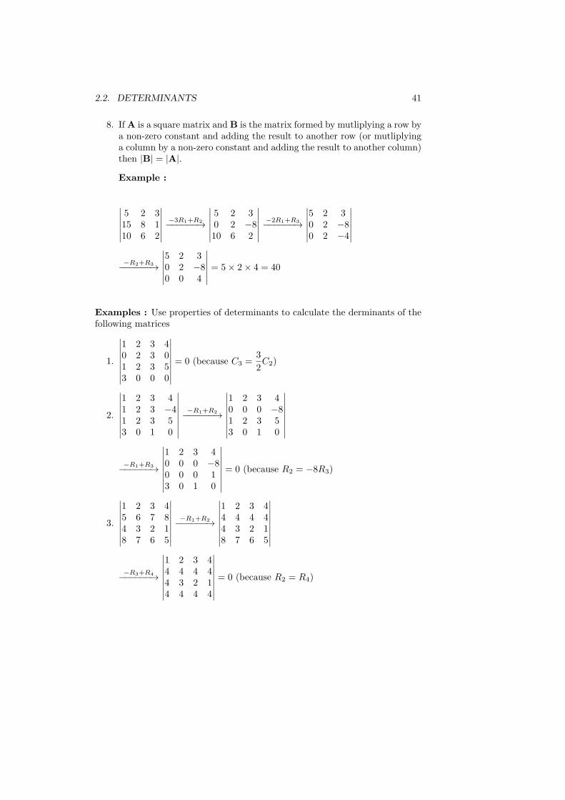
8. IfA is a square matrix and B is the matrix formed by mutliplying a row bya non-zero constant and adding the result to another row (or mutliplyinga column by a non-zero constant and adding the result to another column)then |B| = |A|.
Example :
∣
∣
∣
∣
∣
∣
5 2 315 8 110 6 2
∣
∣
∣
∣
∣
∣
−3R1+R2−−−−−−→
∣
∣
∣
∣
∣
∣
5 2 30 2 −810 6 2
∣
∣
∣
∣
∣
∣
−2R1+R3−−−−−−→
∣
∣
∣
∣
∣
∣
5 2 30 2 −80 2 −4
∣
∣
∣
∣
∣
∣
−R2+R3−−−−−−→
∣
∣
∣
∣
∣
∣
5 2 30 2 −80 0 4
∣
∣
∣
∣
∣
∣
= 5× 2× 4 = 40
Examples : Use properties of determinants to calculate the derminants of thefollowing matrices
1.
∣
∣
∣
∣
∣
∣
∣
∣
1 2 3 40 2 3 01 2 3 53 0 0 0
∣
∣
∣
∣
∣
∣
∣
∣
= 0 (because C3 =3
2C2)
2.
∣
∣
∣
∣
∣
∣
∣
∣
1 2 3 41 2 3 −41 2 3 53 0 1 0
∣
∣
∣
∣
∣
∣
∣
∣
−R1+R2−−−−−−→
∣
∣
∣
∣
∣
∣
∣
∣
1 2 3 40 0 0 −81 2 3 53 0 1 0
∣
∣
∣
∣
∣
∣
∣
∣
−R1+R3−−−−−−→
∣
∣
∣
∣
∣
∣
∣
∣
1 2 3 40 0 0 −80 0 0 13 0 1 0
∣
∣
∣
∣
∣
∣
∣
∣
= 0 (because R2 = −8R3)
3.
∣
∣
∣
∣
∣
∣
∣
∣
1 2 3 45 6 7 84 3 2 18 7 6 5
∣
∣
∣
∣
∣
∣
∣
∣
−R1+R2−−−−−−→
∣
∣
∣
∣
∣
∣
∣
∣
1 2 3 44 4 4 44 3 2 18 7 6 5
∣
∣
∣
∣
∣
∣
∣
∣
−R3+R4−−−−−−→
∣
∣
∣
∣
∣
∣
∣
∣
1 2 3 44 4 4 44 3 2 14 4 4 4
∣
∣
∣
∣
∣
∣
∣
∣
= 0 (because R2 = R4)
42 CHAPTER 2. MATRICES AND DETERMINANTS
Chapter 3
SYSTEMS OF LINEAREQUATIONS
3.1 Systems of Linear Equations
3.2 Cramer’s Rule
3.3 Gauss Elimination Method
3.4 Gauss-Jordan Method
43
44 CHAPTER 3. SYSTEMS OF LINEAR EQUATIONS
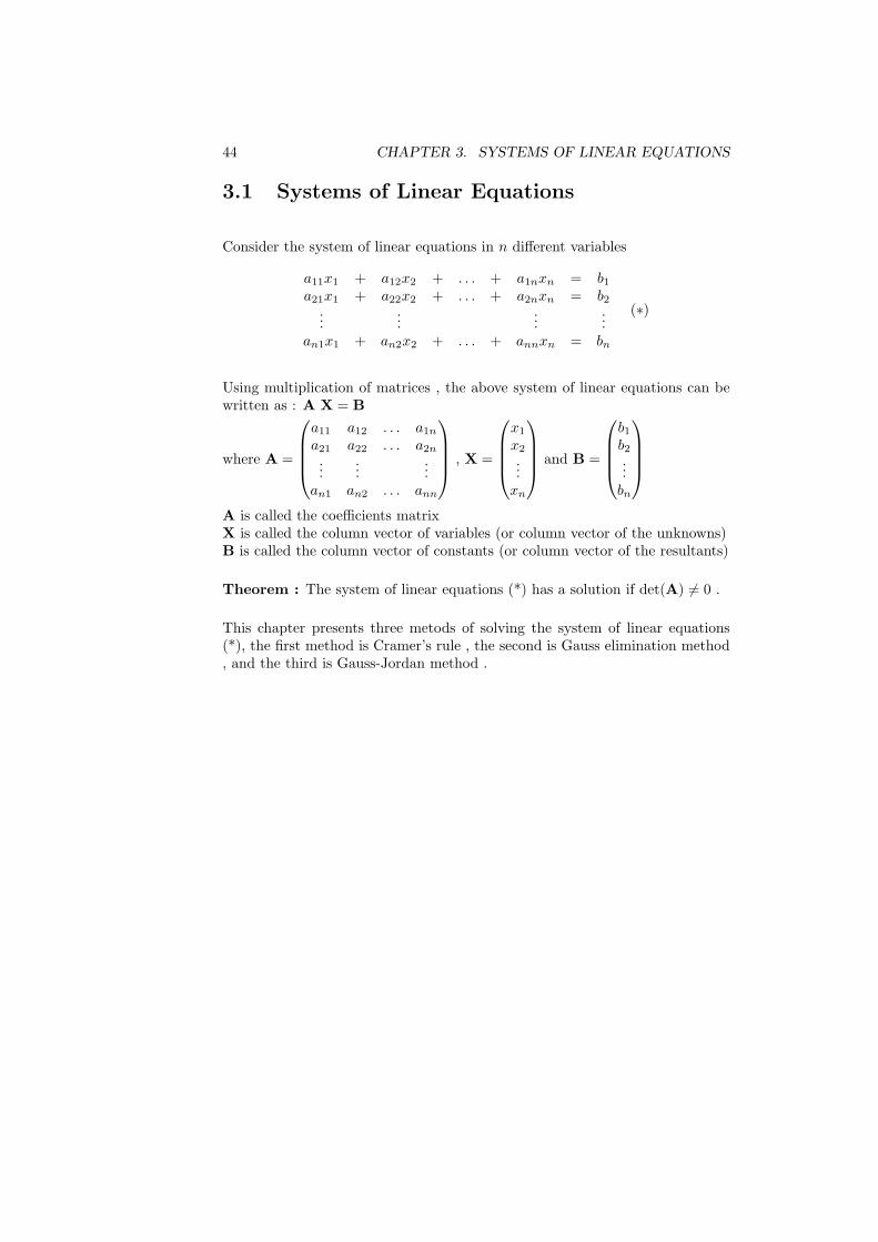
3.1 Systems of Linear Equations
Consider the system of linear equations in n different variables
a11x1 + a12x2 + . . . + a1nxn = b1a21x1 + a22x2 + . . . + a2nxn = b2
......
......
an1x1 + an2x2 + . . . + annxn = bn
(∗)
Using multiplication of matrices , the above system of linear equations can bewritten as : A X = B
where A =
a11 a12 . . . a1na21 a22 . . . a2n...
......
an1 an2 . . . ann
, X =
x1
x2
...xn
and B =
b1b2...bn
A is called the coefficients matrixX is called the column vector of variables (or column vector of the unknowns)B is called the column vector of constants (or column vector of the resultants)
Theorem : The system of linear equations (*) has a solution if det(A) 6= 0 .
This chapter presents three metods of solving the system of linear equations(*), the first method is Cramer’s rule , the second is Gauss elimination method, and the third is Gauss-Jordan method .
3.2. CRAMER’S RULE 45
3.2 Cramer’s rule
Consider the system of linear equations in n different variables
a11x1 + a12x2 + . . . + a1nxn = b1a21x1 + a22x2 + . . . + a2nxn = b2
......
......
an1x1 + an2x2 + . . . + annxn = bn
(∗)
A X = B
where A =
a11 a12 . . . a1na21 a22 . . . a2n...
......
an1 an2 . . . ann
, X =
x1
x2
...xn
and B =
b1b2...bn
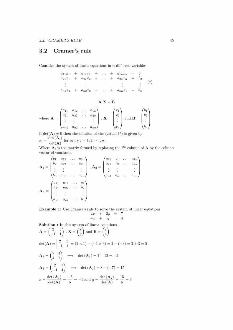
If det(A) 6= 0 then the solution of the system (*) is given by
xi =det (Ai)
det(A)for every i = 1, 2, · · · , n .
Where Ai is the matrix formed by replacing the ith column of A by the columnvector of constants.
A1 =
b1 a12 . . . a1nb2 a22 . . . a2n...
......
bn an2 . . . ann
, A2 =
a11 b1 . . . a1na21 b2 . . . a2n...
......
an1 bn . . . ann
An =
a11 a12 . . . b1a21 a22 . . . b2...
......
an1 an2 . . . bn
Example 1: Use Cramer’s rule to solve the system of linear equations2x + 3y = 7−x + y = 4
Solution : In this system of linear equations
A =
(
2 3−1 1
)
, X =
(
x
y
)
and B =
(
74
)
det(A) =
∣
∣
∣
∣
2 3−1 1
∣
∣
∣
∣
= (2× 1)− (−1× 3) = 2− (−3) = 2 + 3 = 5
A1 =
(
7 34 1
)
=⇒ det (A1) = 7− 12 = −5
A2 =
(
2 7−1 4
)
=⇒ det (A2) = 8− (−7) = 15
x =det (A1)
det(A)=
−5
5= −1 and y =
det (A2)
det(A)=
15
5= 3
46 CHAPTER 3. SYSTEMS OF LINEAR EQUATIONS
The solution of the system of linear equations is
(
x
y
)
=
(
−13
)
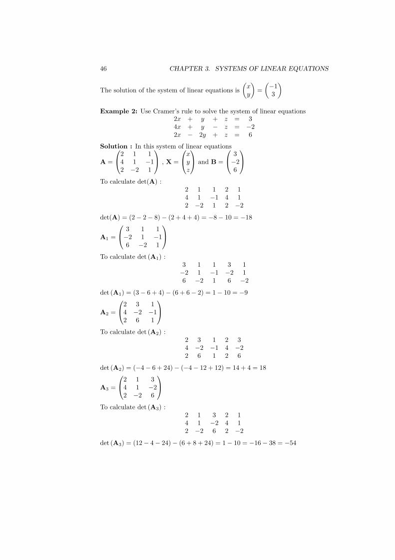
Example 2: Use Cramer’s rule to solve the system of linear equations2x + y + z = 34x + y − z = −22x − 2y + z = 6
Solution : In this system of linear equations
A =
2 1 14 1 −12 −2 1
, X =
x
y
z
and B =
3−26
To calculate det(A) :2 1 1 2 14 1 −1 4 12 −2 1 2 −2
det(A) = (2− 2− 8)− (2 + 4 + 4) = −8− 10 = −18
A1 =
3 1 1−2 1 −16 −2 1
To calculate det (A1) :3 1 1 3 1−2 1 −1 −2 16 −2 1 6 −2
det (A1) = (3− 6 + 4)− (6 + 6− 2) = 1− 10 = −9
A2 =
2 3 14 −2 −12 6 1
To calculate det (A2) :2 3 1 2 34 −2 −1 4 −22 6 1 2 6
det (A2) = (−4− 6 + 24)− (−4− 12 + 12) = 14 + 4 = 18
A3 =
2 1 34 1 −22 −2 6
To calculate det (A3) :2 1 3 2 14 1 −2 4 12 −2 6 2 −2
det (A3) = (12− 4− 24)− (6 + 8 + 24) = 1− 10 = −16− 38 = −54
3.2. CRAMER’S RULE 47
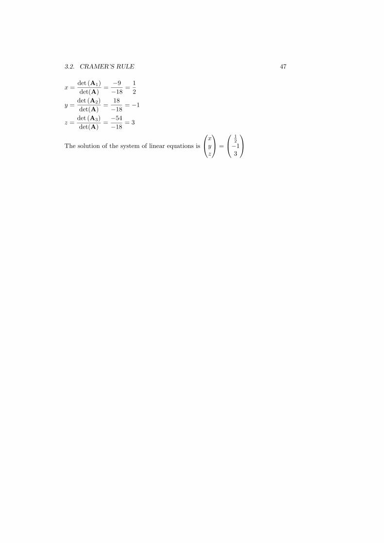
x =det (A1)
det(A)=
−9
−18=
1
2
y =det (A2)
det(A)=
18
−18= −1
z =det (A3)
det(A)=
−54
−18= 3
The solution of the system of linear equations is
x
y
z
=
12−13
48 CHAPTER 3. SYSTEMS OF LINEAR EQUATIONS
3.3 Gauss elimination method
Consider the system of linear equations in n different variables
a11x1 + a12x2 + . . . + a1nxn = b1a21x1 + a22x2 + . . . + a2nxn = b2
......
......
an1x1 + an2x2 + . . . + annxn = bn
(∗)
A X = B
where A =
a11 a12 . . . a1na21 a22 . . . a2n...
......
an1 an2 . . . ann
, X =
x1
x2
...xn
and B =
b1b2...bn
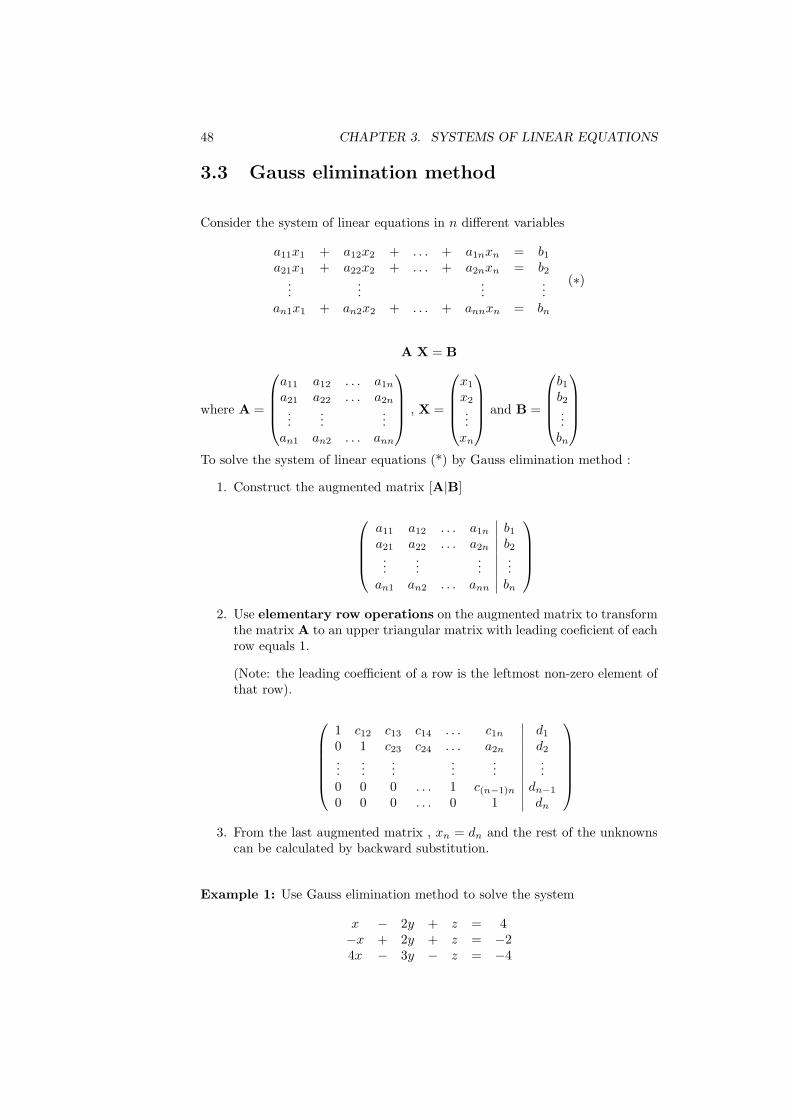
To solve the system of linear equations (*) by Gauss elimination method :
1. Construct the augmented matrix [A|B]
a11 a12 . . . a1n b1a21 a22 . . . a2n b2...
......
...an1 an2 . . . ann bn
2. Use elementary row operations on the augmented matrix to transformthe matrix A to an upper triangular matrix with leading coeficient of eachrow equals 1.
(Note: the leading coefficient of a row is the leftmost non-zero element ofthat row).
1 c12 c13 c14 . . . c1n d10 1 c23 c24 . . . a2n d2...
......
......
...0 0 0 . . . 1 c(n−1)n dn−10 0 0 . . . 0 1 dn
3. From the last augmented matrix , xn = dn and the rest of the unknownscan be calculated by backward substitution.
Example 1: Use Gauss elimination method to solve the system
x − 2y + z = 4−x + 2y + z = −24x − 3y − z = −4
3.3. GAUSS ELIMINATION METHOD 49
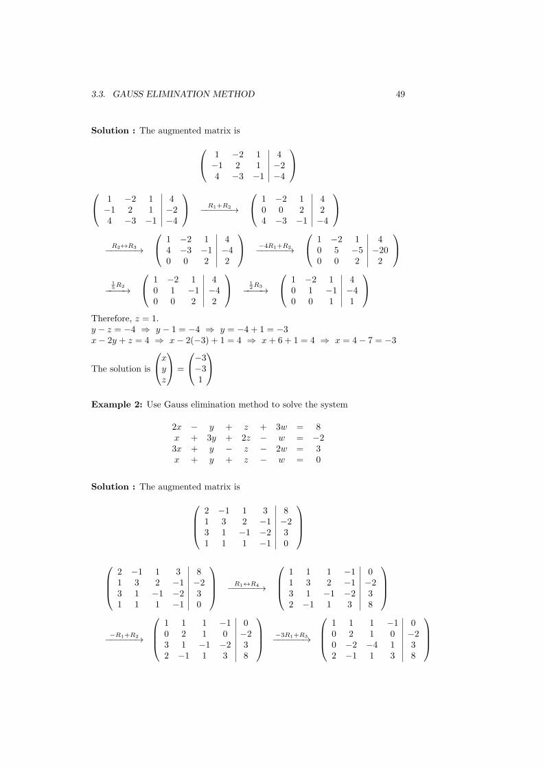
Solution : The augmented matrix is
1 −2 1 4−1 2 1 −24 −3 −1 −4
1 −2 1 4−1 2 1 −24 −3 −1 −4
R1+R2−−−−−−→
1 −2 1 40 0 2 24 −3 −1 −4
R2↔R3−−−−−−→
1 −2 1 44 −3 −1 −40 0 2 2
−4R1+R2−−−−−−→
1 −2 1 40 5 −5 −200 0 2 2
1
5R2−−−−→
1 −2 1 40 1 −1 −40 0 2 2
1
2R3−−−−→
1 −2 1 40 1 −1 −40 0 1 1
Therefore, z = 1.y − z = −4 ⇒ y − 1 = −4 ⇒ y = −4 + 1 = −3x− 2y + z = 4 ⇒ x− 2(−3) + 1 = 4 ⇒ x+ 6 + 1 = 4 ⇒ x = 4− 7 = −3
The solution is
x
y
z
=
−3−31
Example 2: Use Gauss elimination method to solve the system
2x − y + z + 3w = 8x + 3y + 2z − w = −23x + y − z − 2w = 3x + y + z − w = 0
Solution : The augmented matrix is
2 −1 1 3 81 3 2 −1 −23 1 −1 −2 31 1 1 −1 0
2 −1 1 3 81 3 2 −1 −23 1 −1 −2 31 1 1 −1 0
R1↔R4−−−−−−→
1 1 1 −1 01 3 2 −1 −23 1 −1 −2 32 −1 1 3 8
−R1+R2−−−−−−→
1 1 1 −1 00 2 1 0 −23 1 −1 −2 32 −1 1 3 8
−3R1+R3−−−−−−→
1 1 1 −1 00 2 1 0 −20 −2 −4 1 32 −1 1 3 8
50 CHAPTER 3. SYSTEMS OF LINEAR EQUATIONS
−2R1+R4−−−−−−→
1 1 1 −1 00 2 1 0 −20 −2 −4 1 30 −3 −1 5 8
R2+R3−−−−−−→
1 1 1 −1 00 2 1 0 −20 0 −3 1 10 −3 −1 5 8
2R4−−−−→
1 1 1 −1 00 2 1 0 −20 0 −3 1 10 −6 −2 10 16
3R2+R4−−−−−−→
1 1 1 −1 00 2 1 0 −20 0 −3 1 10 0 1 10 10
3R4−−−−→
1 1 1 −1 00 2 1 0 −20 0 −3 1 10 0 3 30 30
R3+R4−−−−−−→
1 1 1 −1 00 2 1 0 −20 0 −3 1 10 0 0 31 31
1
2R2−−−−→
1 1 1 −1 00 1 1
2 0 −10 0 −3 1 10 0 0 31 31
−1
3R3−−−−→
1 1 1 −1 00 1 1
2 0 −10 0 1 − 1
3 − 13
0 0 0 31 31
1
31R4−−−−→
1 1 1 −1 00 1 1
2 0 −10 0 1 − 1
3 − 13
0 0 0 1 1
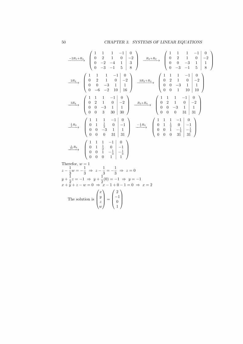
Therefor, w = 1
z − 1
3w = −1
3⇒ z − 1
3= −1
3⇒ z = 0
y +1
2z = −1 ⇒ y +
1
2(0) = −1 ⇒ y = −1
x+ y + z − w = 0 ⇒ x− 1 + 0− 1 = 0 ⇒ x = 2
The solution is
x
y
z
w
=
2−101
3.4. GAUSS-JORDAN METHOD 51
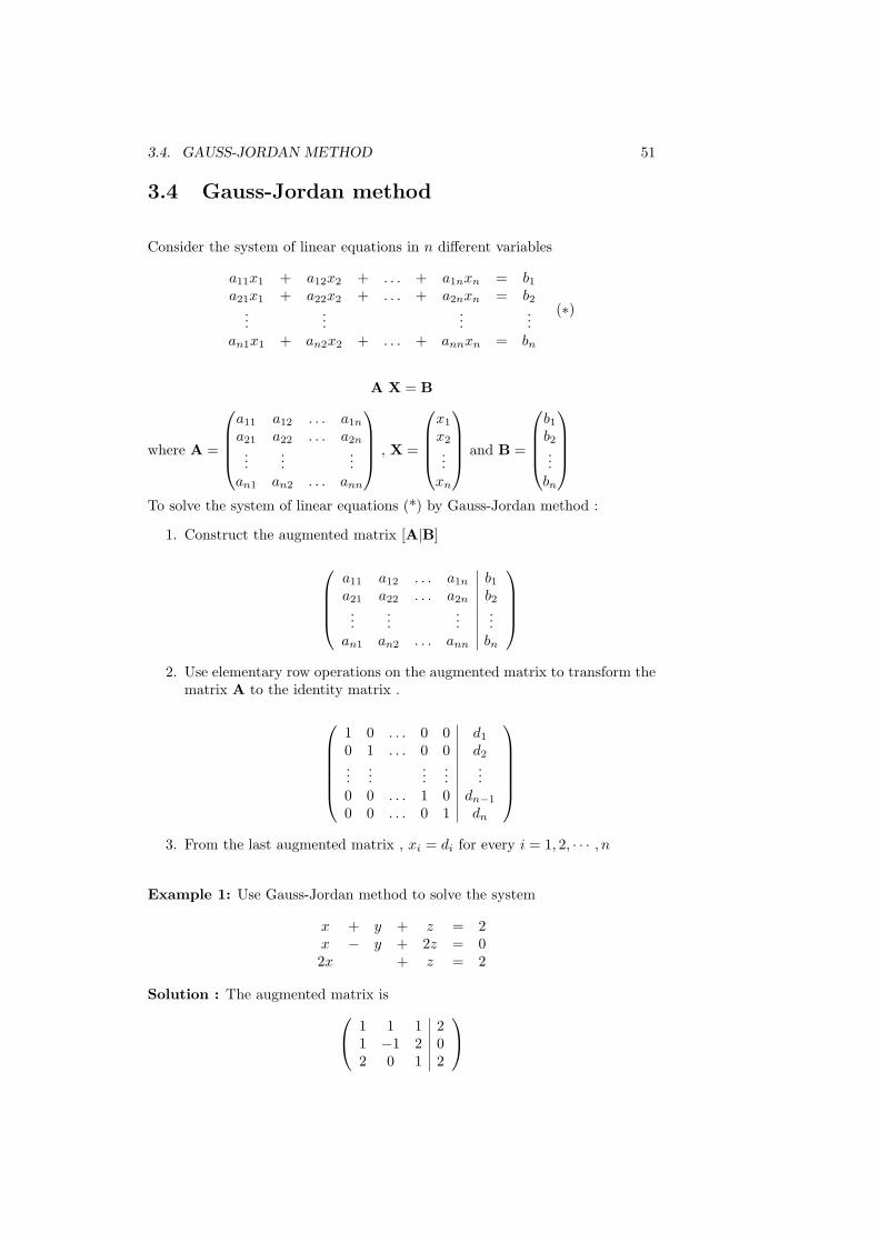
3.4 Gauss-Jordan method
Consider the system of linear equations in n different variables
a11x1 + a12x2 + . . . + a1nxn = b1a21x1 + a22x2 + . . . + a2nxn = b2
......
......
an1x1 + an2x2 + . . . + annxn = bn
(∗)
A X = B
where A =
a11 a12 . . . a1na21 a22 . . . a2n...
......
an1 an2 . . . ann
, X =
x1
x2
...xn
and B =
b1b2...bn
To solve the system of linear equations (*) by Gauss-Jordan method :
1. Construct the augmented matrix [A|B]
a11 a12 . . . a1n b1a21 a22 . . . a2n b2...
......
...an1 an2 . . . ann bn
2. Use elementary row operations on the augmented matrix to transform thematrix A to the identity matrix .
1 0 . . . 0 0 d10 1 . . . 0 0 d2...
......
......
0 0 . . . 1 0 dn−10 0 . . . 0 1 dn
3. From the last augmented matrix , xi = di for every i = 1, 2, · · · , n
Example 1: Use Gauss-Jordan method to solve the system
x + y + z = 2x − y + 2z = 02x + z = 2
Solution : The augmented matrix is
1 1 1 21 −1 2 02 0 1 2
52 CHAPTER 3. SYSTEMS OF LINEAR EQUATIONS
1 1 1 21 −1 2 02 0 1 2
−R1+R2−−−−−−→
1 1 1 20 −2 1 −22 0 1 2
−2R1+R3−−−−−−→
1 1 1 20 −2 1 −20 −2 −1 −2
−R2+R3−−−−−−→
1 1 1 20 −2 1 −20 0 −2 0
−1
2R3−−−−→
1 1 1 20 −2 1 −20 0 1 0
−R3+R2−−−−−−→
1 1 1 20 −2 0 −20 0 1 0
−R3+R1−−−−−−→
1 1 0 20 −2 0 −20 0 1 0
−1
2R2−−−−→
1 1 0 20 1 0 10 0 1 0
−R2+R1−−−−−−→
1 0 0 10 1 0 10 0 1 0
Therefore , x = 1 , y = 1 and z = 0.
The solution is
x
y
z
=
110
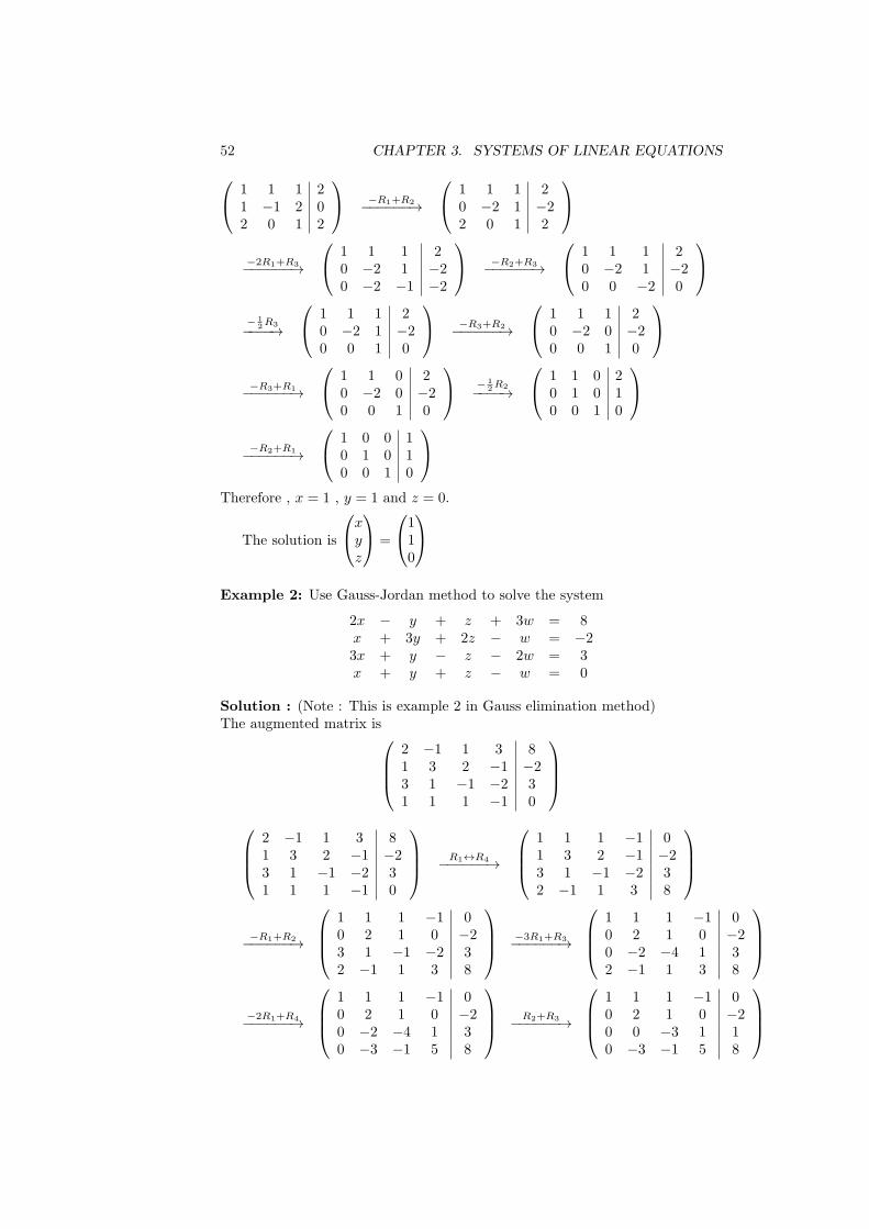
Example 2: Use Gauss-Jordan method to solve the system
2x − y + z + 3w = 8x + 3y + 2z − w = −23x + y − z − 2w = 3x + y + z − w = 0
Solution : (Note : This is example 2 in Gauss elimination method)The augmented matrix is
2 −1 1 3 81 3 2 −1 −23 1 −1 −2 31 1 1 −1 0
2 −1 1 3 81 3 2 −1 −23 1 −1 −2 31 1 1 −1 0
R1↔R4−−−−−−→
1 1 1 −1 01 3 2 −1 −23 1 −1 −2 32 −1 1 3 8
−R1+R2−−−−−−→
1 1 1 −1 00 2 1 0 −23 1 −1 −2 32 −1 1 3 8
−3R1+R3−−−−−−→
1 1 1 −1 00 2 1 0 −20 −2 −4 1 32 −1 1 3 8
−2R1+R4−−−−−−→
1 1 1 −1 00 2 1 0 −20 −2 −4 1 30 −3 −1 5 8
R2+R3−−−−−−→
1 1 1 −1 00 2 1 0 −20 0 −3 1 10 −3 −1 5 8
3.4. GAUSS-JORDAN METHOD 53
2R4−−−−→
1 1 1 −1 00 2 1 0 −20 0 −3 1 10 −6 −2 10 16
3R2+R4−−−−−−→
1 1 1 −1 00 2 1 0 −20 0 −3 1 10 0 1 10 10
3R4−−−−→
1 1 1 −1 00 2 1 0 −20 0 −3 1 10 0 3 30 30
R3+R4−−−−−−→
1 1 1 −1 00 2 1 0 −20 0 −3 1 10 0 0 31 31
1
31R4−−−−→
1 1 1 −1 00 2 1 0 −20 0 −3 1 10 0 0 1 1
−R4+R3−−−−−−→
1 1 1 −1 00 2 1 0 −20 0 −3 0 00 0 0 1 1
R4+R1−−−−−−→
1 1 1 0 10 2 1 0 −20 0 −3 0 00 0 0 1 1
−1
3R3−−−−→
1 1 1 0 10 2 1 0 −20 0 1 0 00 0 0 1 1
−R3+R2−−−−−−→
1 1 1 0 10 2 0 0 −20 0 1 0 00 0 0 1 1
−R3+R1−−−−−−→
1 1 0 0 10 2 0 0 −20 0 1 0 00 0 0 1 1
1
2R2−−−−→
1 1 0 0 10 1 0 0 −10 0 1 0 00 0 0 1 1
−R2+R1−−−−−−→
1 0 0 0 20 1 0 0 −10 0 1 0 00 0 0 1 1
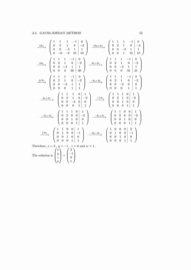
Therefore, x = 2 , y = −1 , z = 0 and w = 1.
The solution is
x
y
z
w
=
2−101
54 CHAPTER 3. SYSTEMS OF LINEAR EQUATIONS
Chapter 4
INTEGRATION
4.1 Indefinite integral
4.2 Integration by substitution
4.3 Integration by parts
4.4 Integration of rational functions
(Method of partial fractions)
55
56 CHAPTER 4. INTEGRATION
4.1 Indefinite integral
Definition (Antiderivative): A function G is called an antiderivative of thefunction f on the interval [a, b] if G′(x) = f(x) for all x ∈ [a, b].
Examples : What is the antiderivative of the following functions
1. f(x) = 2x .
2. f(x) = cosx .
3. f(x) = sec2 x
4. f(x) =1
x
5. f(x) = ex
Solution :
1. G(x) = x2 + c
G′(x) =d
dxG(x) =
d
dx
(
x2 + c)
= 2x+ 0 = 2x
2. G(x) = sinx+ c
G′(x) =d
dxG(x) =
d
dx(sinx+ c) = cosx
3. G(x) = tanx+ c
G′(x) =d
dxG(x) =
d
dx(tanx+ c) = sec2 x
4. G(x) = ln |x|+ c
G′(x) =d
dxG(x) =
d
dx(ln |x|+ c) =
1
x
5. G(x) = ex + c
G′(x) =d
dxG(x) =
d
dx(ex + c) = ex
Note: If G1(x) and G2(x) are both antiderivatives of the function f(x) thenG1(x)−G2(x) = constant.
Definition (indefinite integral): If G(x) is the antiderivative of f(x) then∫
f(x) dx = G(x)+c ,
∫
f(x) dx is called the indefinite integral of the function
f(x).
4.1. INDEFINITE INTEGRAL 57
Basic Rules of integration :
1.
∫
1 dx = x+ c
2.
∫
xn dx =xn+1
n+ 1+ c , where n 6= −1
3.
∫
cosx dx = sinx+ c
4.
∫
sinx dx = − cosx+ c
5.
∫
sec2 x dx = tanx+ c
6.
∫
csc2 x dx = − cotx+ c
7.
∫
secx tanx dx = secx+ c
8.
∫
cscx cotx = − cscx+ c
9.
∫
1
xdx = ln |x|+ c
10.
∫
ex dx = ex + c
11.
∫
1√1− x2
dx = sin−1 x+ c , where |x| < 1
12.
∫
1
1 + x2dx = tan−1 x+ c
13.
∫
1
x√x2 − 1
dx = sec−1 x+ c , where |x| > 1
Properties of indefinite integral :
1.
∫
k f(x) dx = k
∫
f(x) dx , where k ∈ R
2.
∫
(f(x)± g(x)) dx =
∫
f(x) dx±∫
g(x) dx
58 CHAPTER 4. INTEGRATION
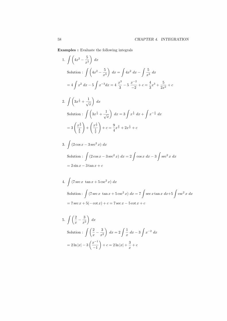
Examples : Evaluate the following integrals
1.
∫ (
4x2 − 5
x3
)
dx
Solution :
∫ (
4x2 − 5
x3
)
dx =
∫
4x2 dx−∫
5
x3dx
= 4
∫
x2 dx− 5
∫
x−3dx = 4x3
3− 5
x−2
−2+ c =
4
3x3 +
5
2x2+ c
2.
∫ (
3x1
3 +1√x
)
dx
Solution :
∫ (
3x1
3 +1√x
)
dx = 3
∫
x1
3 dx+
∫
x−1
2 dx
= 3
(
x4
3
43
)
+
(
x1
2
12
)
+ c =9
4x
4
3 + 2x1
2 + c
3.
∫
(2 cosx− 3 sec2 x) dx
Solution :
∫
(2 cosx− 3 sec2 x) dx = 2
∫
cosx dx− 3
∫
sec2 x dx
= 2 sinx− 3 tanx+ c
4.
∫
(7 secx tanx+ 5 csc2 x) dx
Solution :
∫
(7 secx tanx+ 5 csc2 x) dx = 7
∫
secx tanx dx+5
∫
csc2 x dx
= 7 secx+ 5(− cotx) + c = 7 secx− 5 cotx+ c
5.
∫ (
2
x− 3
x2
)
dx
Solution :
∫ (
2
x− 3
x2
)
dx = 2
∫
1
xdx− 3
∫
x−2 dx
= 2 ln |x| − 3
(
x−1
−1
)
+ c = 2 ln |x|+ 3
x+ c
4.1. INDEFINITE INTEGRAL 59
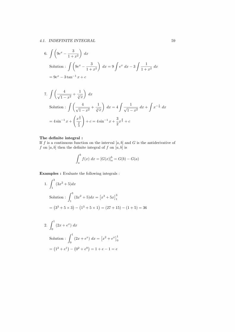
6.
∫ (
9ex − 3
1 + x2
)
dx
Solution :
∫ (
9ex − 3
1 + x2
)
dx = 9
∫
ex dx− 3
∫
1
1 + x2dx
= 9ex − 3 tan−1 x+ c
7.
∫ (
4√1− x2
+13√x
)
dx
Solution :
∫ (
4√1− x2
+13√x
)
dx = 4
∫
1√1− x2
dx+
∫
x−1
3 dx
= 4 sin−1 x+
(
x2
3
23
)
+ c = 4 sin−1 x+3
2x
2
3 + c
The definite integral :If f is a continuous function on the interval [a, b] and G is the antiderivative off on [a, b] then the definite integral of f on [a, b] is
∫ b
a
f(x) dx = [G(x)]b
a = G(b)−G(a)
Examples : Evaluate the following integrals :
1.
∫ 3
1
(3x2 + 5)dx
Solution :
∫ 3
1
(3x2 + 5)dx =[
x3 + 5x]3
1
=(
33 + 5× 3)
−(
13 + 5× 1)
= (27 + 15)− (1 + 5) = 36
2.
∫ 1
0
(2x+ ex) dx
Solution :
∫ 1
0
(2x+ ex) dx =[
x2 + ex]1
0
=(
12 + e1)
−(
02 + e0)
= 1 + e− 1 = e
60 CHAPTER 4. INTEGRATION
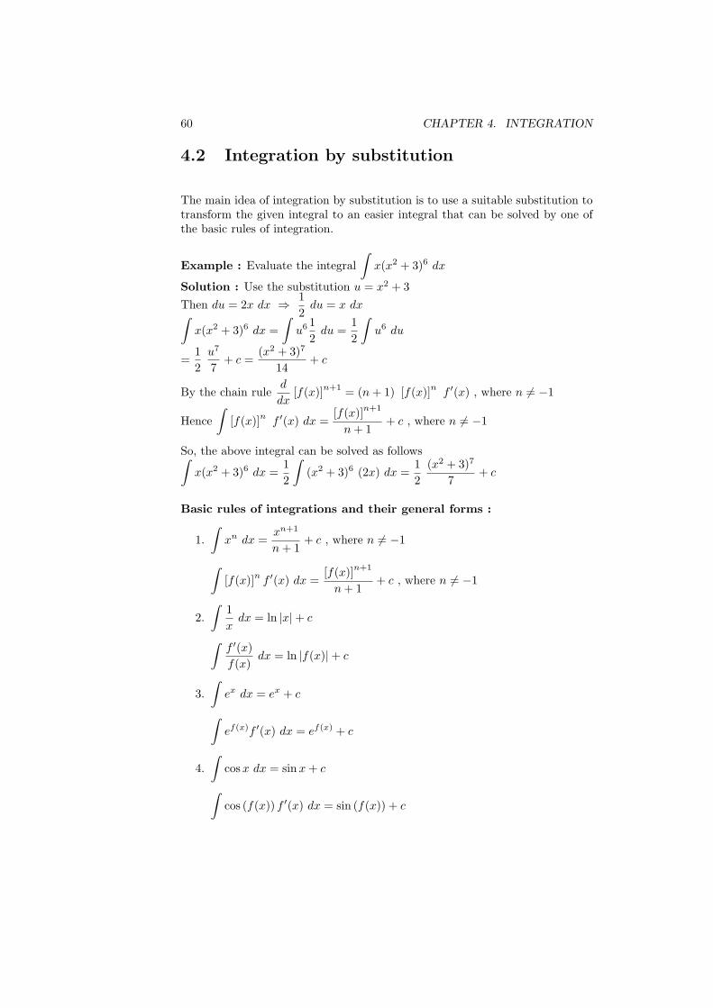
4.2 Integration by substitution
The main idea of integration by substitution is to use a suitable substitution totransform the given integral to an easier integral that can be solved by one ofthe basic rules of integration.
Example : Evaluate the integral
∫
x(x2 + 3)6 dx
Solution : Use the substitution u = x2 + 3
Then du = 2x dx ⇒ 1
2du = x dx
∫
x(x2 + 3)6 dx =
∫
u6 1
2du =
1
2
∫
u6 du
=1
2
u7
7+ c =
(x2 + 3)7
14+ c
By the chain ruled
dx[f(x)]
n+1= (n+ 1) [f(x)]
nf ′(x) , where n 6= −1
Hence
∫
[f(x)]n
f ′(x) dx =[f(x)]
n+1
n+ 1+ c , where n 6= −1
So, the above integral can be solved as follows∫
x(x2 + 3)6 dx =1
2
∫
(x2 + 3)6 (2x) dx =1
2
(x2 + 3)7
7+ c
Basic rules of integrations and their general forms :
1.
∫
xn dx =xn+1
n+ 1+ c , where n 6= −1
∫
[f(x)]nf ′(x) dx =
[f(x)]n+1
n+ 1+ c , where n 6= −1
2.
∫
1
xdx = ln |x|+ c
∫
f ′(x)
f(x)dx = ln |f(x)|+ c
3.
∫
ex dx = ex + c
∫
ef(x)f ′(x) dx = ef(x) + c
4.
∫
cosx dx = sinx+ c
∫
cos (f(x)) f ′(x) dx = sin (f(x)) + c
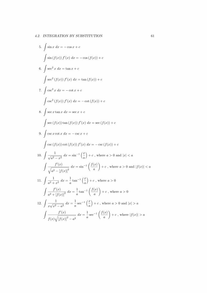
4.2. INTEGRATION BY SUBSTITUTION 61
5.
∫
sinx dx = − cosx+ c
∫
sin (f(x)) f ′(x) dx = − cos (f(x)) + c
6.
∫
sec2 x dx = tanx+ c
∫
sec2 (f(x)) f ′(x) dx = tan (f(x)) + c
7.
∫
csc2 x dx = − cotx+ c
∫
csc2 (f(x)) f ′(x) dx = − cot (f(x)) + c
8.
∫
secx tanx dx = secx+ c
∫
sec (f(x)) tan (f(x)) f ′(x) dx = sec (f(x)) + c
9.
∫
cscx cotx dx = − cscx+ c
∫
csc (f(x)) cot (f(x)) f ′(x) dx = − csc (f(x)) + c
10.
∫
1√a2 − x2
dx = sin−1(x
a
)
+ c , where a > 0 and |x| < a
∫
f ′(x)√
a2 − [f(x)]2dx = sin−1
(
f(x)
a
)
+ c , where a > 0 and |f(x)| < a
11.
∫
1
a2 + x2dx =
1
atan−1
(x
a
)
+ c , where a > 0
∫
f ′(x)
a2 + [f(x)]2 dx =
1
atan−1
(
f(x)
a
)
+ c , where a > 0
12.
∫
1
x√x2 − a2
dx =1
asec−1
(x
a
)
+ c , where a > 0 and |x| > a
∫
f ′(x)
f(x)
√
[f(x)]2 − a2
dx =1
asec−1
(
f(x)
a
)
+ c , where |f(x)| > a
62 CHAPTER 4. INTEGRATION
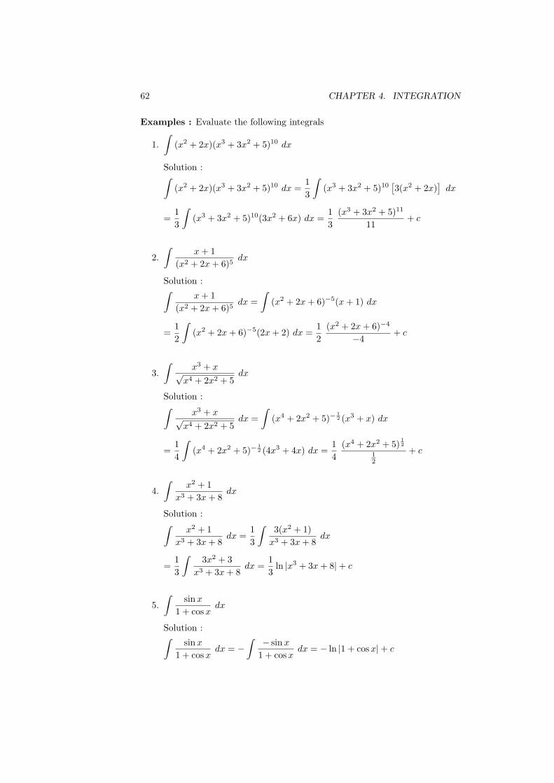
Examples : Evaluate the following integrals
1.
∫
(x2 + 2x)(x3 + 3x2 + 5)10 dx
Solution :∫
(x2 + 2x)(x3 + 3x2 + 5)10 dx =1
3
∫
(x3 + 3x2 + 5)10[
3(x2 + 2x)]
dx
=1
3
∫
(x3 + 3x2 + 5)10(3x2 + 6x) dx =1
3
(x3 + 3x2 + 5)11
11+ c
2.
∫
x+ 1
(x2 + 2x+ 6)5dx
Solution :∫
x+ 1
(x2 + 2x+ 6)5dx =
∫
(x2 + 2x+ 6)−5(x+ 1) dx
=1
2
∫
(x2 + 2x+ 6)−5(2x+ 2) dx =1
2
(x2 + 2x+ 6)−4
−4+ c
3.
∫
x3 + x√x4 + 2x2 + 5
dx
Solution :∫
x3 + x√x4 + 2x2 + 5
dx =
∫
(x4 + 2x2 + 5)−1
2 (x3 + x) dx
=1
4
∫
(x4 + 2x2 + 5)−1
2 (4x3 + 4x) dx =1
4
(x4 + 2x2 + 5)1
2
12
+ c
4.
∫
x2 + 1
x3 + 3x+ 8dx
Solution :∫
x2 + 1
x3 + 3x+ 8dx =
1
3
∫
3(x2 + 1)
x3 + 3x+ 8dx
=1
3
∫
3x2 + 3
x3 + 3x+ 8dx =
1
3ln |x3 + 3x+ 8|+ c
5.
∫
sinx
1 + cosxdx
Solution :∫
sinx
1 + cosxdx = −
∫ − sinx
1 + cosxdx = − ln |1 + cosx|+ c
4.2. INTEGRATION BY SUBSTITUTION 63
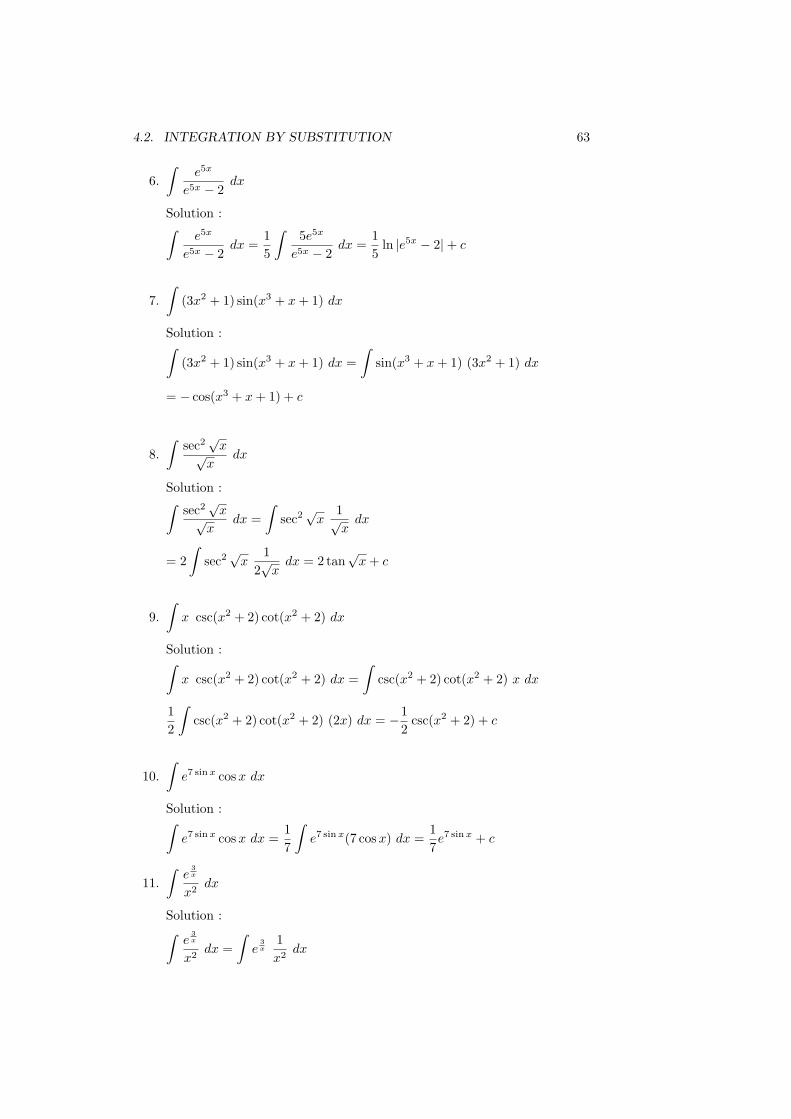
6.
∫
e5x
e5x − 2dx
Solution :∫
e5x
e5x − 2dx =
1
5
∫
5e5x
e5x − 2dx =
1
5ln |e5x − 2|+ c
7.
∫
(3x2 + 1) sin(x3 + x+ 1) dx
Solution :∫
(3x2 + 1) sin(x3 + x+ 1) dx =
∫
sin(x3 + x+ 1) (3x2 + 1) dx
= − cos(x3 + x+ 1) + c
8.
∫
sec2√x√
xdx
Solution :∫
sec2√x√
xdx =
∫
sec2√x
1√x
dx
= 2
∫
sec2√x
1
2√x
dx = 2 tan√x+ c
9.
∫
x csc(x2 + 2) cot(x2 + 2) dx
Solution :∫
x csc(x2 + 2) cot(x2 + 2) dx =
∫
csc(x2 + 2) cot(x2 + 2) x dx
1
2
∫
csc(x2 + 2) cot(x2 + 2) (2x) dx = −1
2csc(x2 + 2) + c
10.
∫
e7 sin x cosx dx
Solution :∫
e7 sin x cosx dx =1
7
∫
e7 sin x(7 cosx) dx =1
7e7 sin x + c
11.
∫
e3
x
x2dx
Solution :∫
e3
x
x2dx =
∫
e3
x
1
x2dx
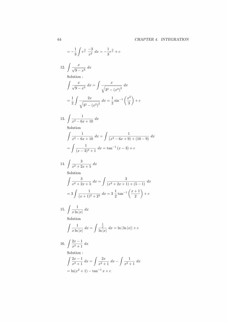
64 CHAPTER 4. INTEGRATION
= −1
3
∫
e3
x
−3
x2dx = −1
3e
3
x + c
12.
∫
x√9− x4
dx
Solution :∫
x√9− x4
dx =
∫
x√
32 − (x2)2dx
=1
2
∫
2x√
32 − (x2)2dx =
1
2sin−1
(
x2
3
)
+ c
13.
∫
1
x2 − 6x+ 10dx
Solution∫
1
x2 − 6x+ 10dx =
∫
1
(x2 − 6x+ 9) + (10− 9)dx
=
∫
1
(x− 3)2 + 1dx = tan−1 (x− 3) + c
14.
∫
3
x2 + 2x+ 5dx
Solution∫
3
x2 + 2x+ 5dx =
∫
3
(x2 + 2x+ 1) + (5− 1)dx
= 3
∫
1
(x+ 1)2 + 22dx = 3
1
2tan−1
(
x+ 1
2
)
+ c
15.
∫
1
x ln |x| dx
Solution∫
1
x ln |x| dx =
∫ 1x
ln |x| dx = ln | ln |x||+ c
16.
∫
2x− 1
x2 + 1dx
Solution :∫
2x− 1
x2 + 1dx =
∫
2x
x2 + 1dx−
∫
1
x2 + 1dx
= ln(x2 + 1)− tan−1 x+ c
4.3. INTEGRATION BY PARTS 65
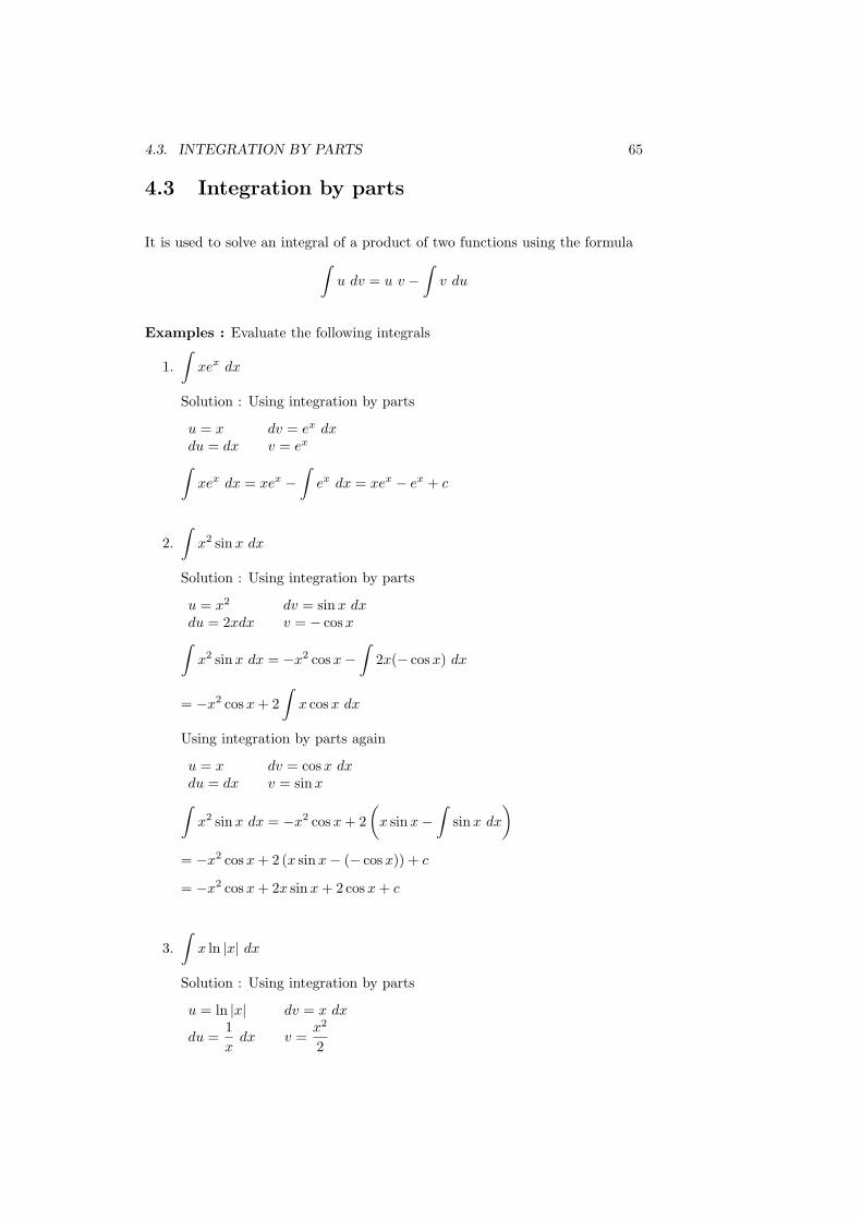
4.3 Integration by parts
It is used to solve an integral of a product of two functions using the formula
∫
u dv = u v −∫
v du
Examples : Evaluate the following integrals
1.
∫
xex dx
Solution : Using integration by parts
u = x dv = ex dx
du = dx v = ex
∫
xex dx = xex −∫
ex dx = xex − ex + c
2.
∫
x2 sinx dx
Solution : Using integration by parts
u = x2 dv = sinx dx
du = 2xdx v = − cosx∫
x2 sinx dx = −x2 cosx−∫
2x(− cosx) dx
= −x2 cosx+ 2
∫
x cosx dx
Using integration by parts again
u = x dv = cosx dx
du = dx v = sinx
∫
x2 sinx dx = −x2 cosx+ 2
(
x sinx−∫
sinx dx
)
= −x2 cosx+ 2 (x sinx− (− cosx)) + c
= −x2 cosx+ 2x sinx+ 2 cosx+ c
3.
∫
x ln |x| dx
Solution : Using integration by parts
u = ln |x| dv = x dx
du =1
xdx v =
x2
2
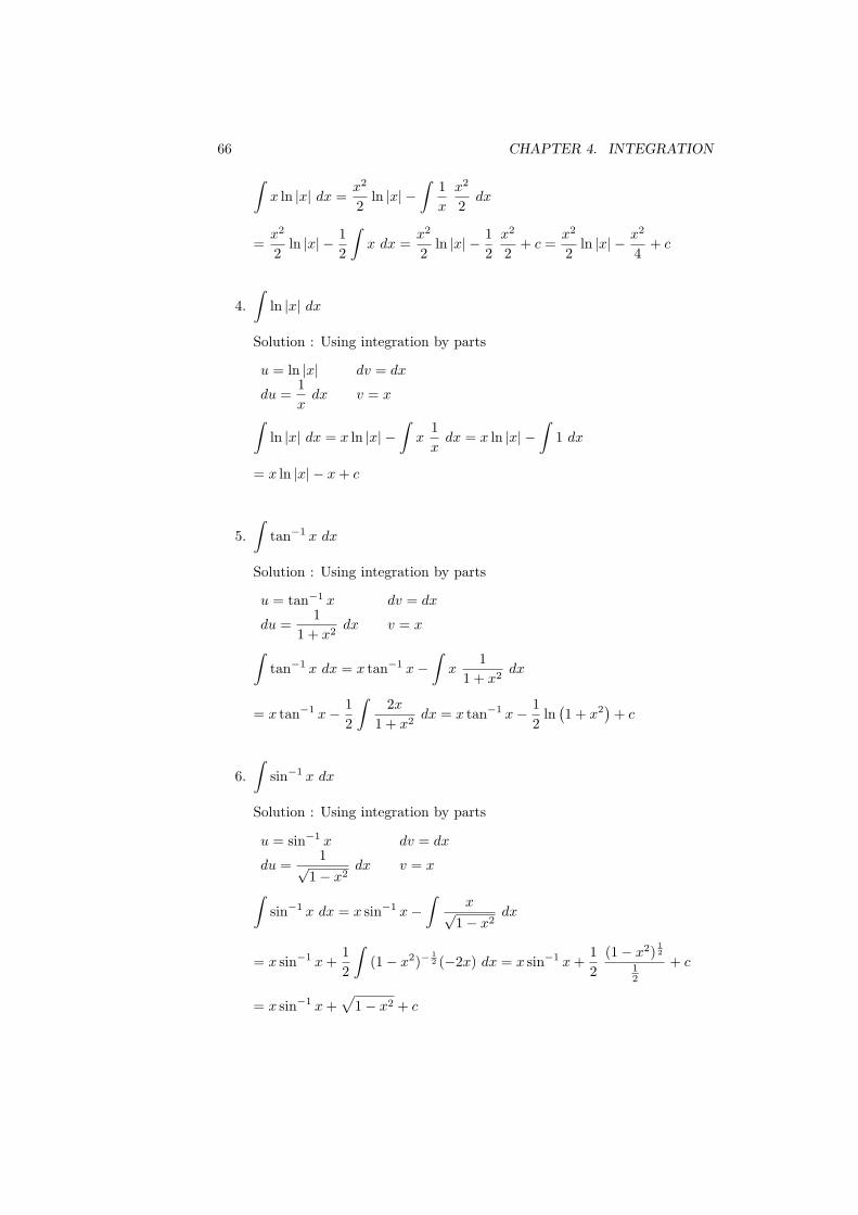
66 CHAPTER 4. INTEGRATION
∫
x ln |x| dx =x2
2ln |x| −
∫
1
x
x2
2dx
=x2
2ln |x| − 1
2
∫
x dx =x2
2ln |x| − 1
2
x2
2+ c =
x2
2ln |x| − x2
4+ c
4.
∫
ln |x| dx
Solution : Using integration by parts
u = ln |x| dv = dx
du =1
xdx v = x
∫
ln |x| dx = x ln |x| −∫
x1
xdx = x ln |x| −
∫
1 dx
= x ln |x| − x+ c
5.
∫
tan−1 x dx
Solution : Using integration by parts
u = tan−1 x dv = dx
du =1
1 + x2dx v = x
∫
tan−1 x dx = x tan−1 x−∫
x1
1 + x2dx
= x tan−1 x− 1
2
∫
2x
1 + x2dx = x tan−1 x− 1
2ln(
1 + x2)
+ c
6.
∫
sin−1 x dx
Solution : Using integration by parts
u = sin−1 x dv = dx
du =1√
1− x2dx v = x
∫
sin−1 x dx = x sin−1 x−∫
x√1− x2
dx
= x sin−1 x+1
2
∫
(1− x2)−1
2 (−2x) dx = x sin−1 x+1
2
(1− x2)1
2
12
+ c
= x sin−1 x+√
1− x2 + c
4.3. INTEGRATION BY PARTS 67
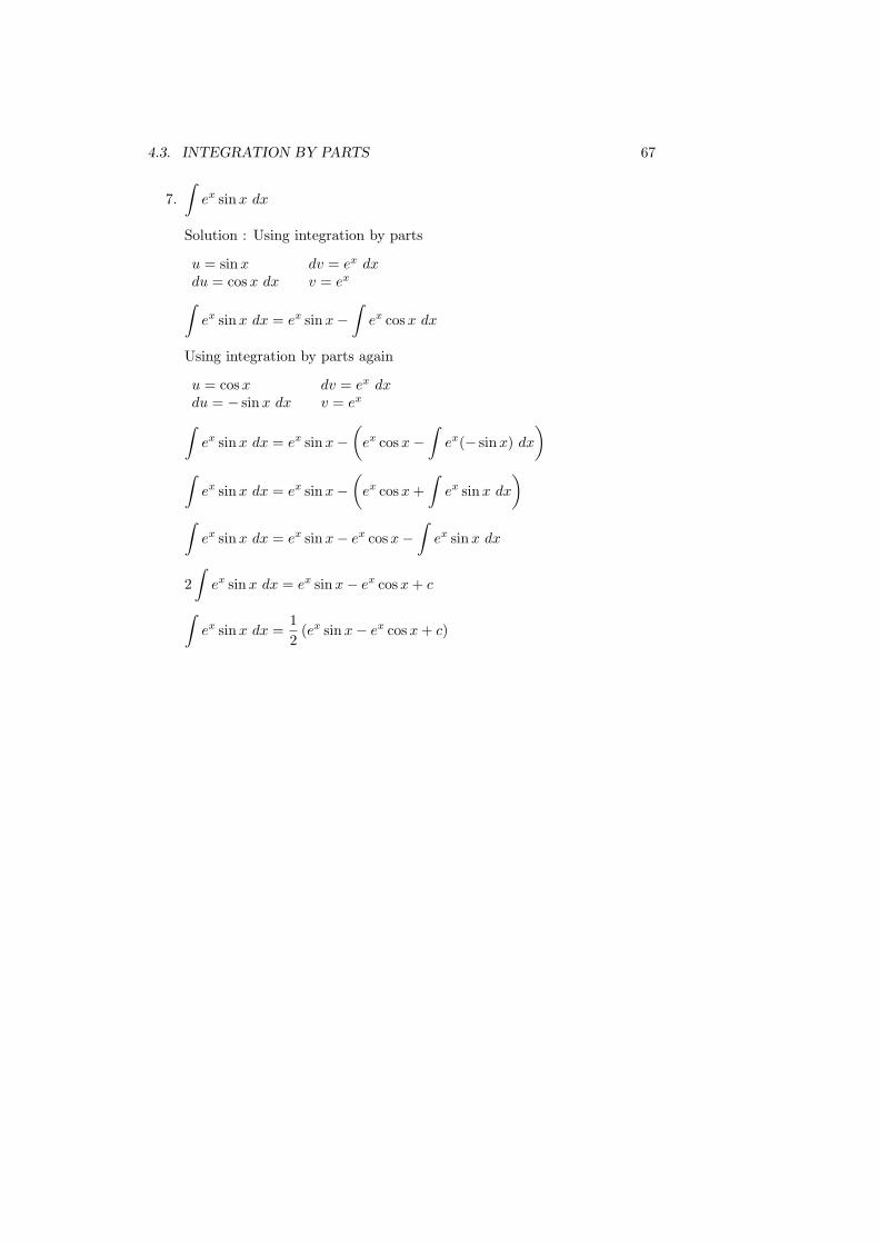
7.
∫
ex sinx dx
Solution : Using integration by parts
u = sinx dv = ex dx
du = cosx dx v = ex
∫
ex sinx dx = ex sinx−∫
ex cosx dx
Using integration by parts again
u = cosx dv = ex dx
du = − sinx dx v = ex
∫
ex sinx dx = ex sinx−(
ex cosx−∫
ex(− sinx) dx
)
∫
ex sinx dx = ex sinx−(
ex cosx+
∫
ex sinx dx
)
∫
ex sinx dx = ex sinx− ex cosx−∫
ex sinx dx
2
∫
ex sinx dx = ex sinx− ex cosx+ c
∫
ex sinx dx =1
2(ex sinx− ex cosx+ c)
68 CHAPTER 4. INTEGRATION
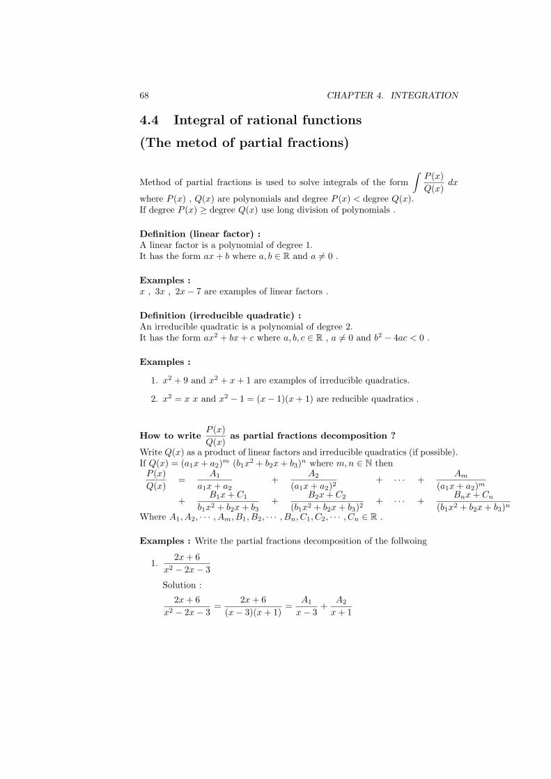
4.4 Integral of rational functions
(The metod of partial fractions)
Method of partial fractions is used to solve integrals of the form
∫
P (x)
Q(x)dx
where P (x) , Q(x) are polynomials and degree P (x) < degree Q(x).If degree P (x) ≥ degree Q(x) use long division of polynomials .
Definition (linear factor) :A linear factor is a polynomial of degree 1.It has the form ax+ b where a, b ∈ R and a 6= 0 .
Examples :x , 3x , 2x− 7 are examples of linear factors .
Definition (irreducible quadratic) :An irreducible quadratic is a polynomial of degree 2.It has the form ax2 + bx+ c where a, b, c ∈ R , a 6= 0 and b2 − 4ac < 0 .
Examples :
1. x2 + 9 and x2 + x+ 1 are examples of irreducible quadratics.
2. x2 = x x and x2 − 1 = (x− 1)(x+ 1) are reducible quadratics .
How to writeP (x)
Q(x)as partial fractions decomposition ?
Write Q(x) as a product of linear factors and irreducible quadratics (if possible).If Q(x) = (a1x+ a2)
m (b1x2 + b2x+ b3)
n where m,n ∈ N thenP (x)
Q(x)=
A1
a1x+ a2+
A2
(a1x+ a2)2+ · · · +
Am
(a1x+ a2)m
+B1x+ C1
b1x2 + b2x+ b3+
B2x+ C2
(b1x2 + b2x+ b3)2+ · · · +
Bnx+ Cn
(b1x2 + b2x+ b3)n
Where A1, A2, · · · , Am, B1, B2, · · · , Bn, C1, C2, · · · , Cn ∈ R .
Examples : Write the partial fractions decomposition of the follwoing
1.2x+ 6
x2 − 2x− 3
Solution :
2x+ 6
x2 − 2x− 3=
2x+ 6
(x− 3)(x+ 1)=
A1
x− 3+
A2
x+ 1
4.4. INTEGRAL OF RATIONAL FUNCTIONS 69
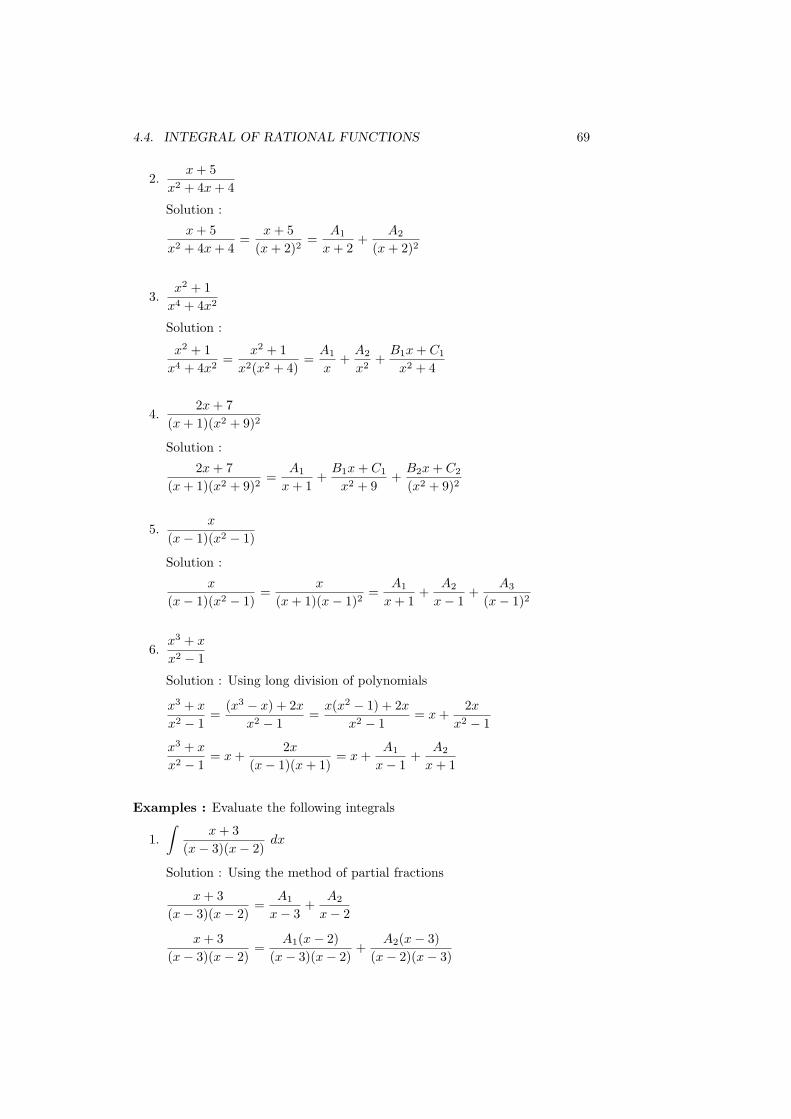
2.x+ 5
x2 + 4x+ 4
Solution :
x+ 5
x2 + 4x+ 4=
x+ 5
(x+ 2)2=
A1
x+ 2+
A2
(x+ 2)2
3.x2 + 1
x4 + 4x2
Solution :
x2 + 1
x4 + 4x2=
x2 + 1
x2(x2 + 4)=
A1
x+
A2
x2+
B1x+ C1
x2 + 4
4.2x+ 7
(x+ 1)(x2 + 9)2
Solution :
2x+ 7
(x+ 1)(x2 + 9)2=
A1
x+ 1+
B1x+ C1
x2 + 9+
B2x+ C2
(x2 + 9)2
5.x
(x− 1)(x2 − 1)
Solution :
x
(x− 1)(x2 − 1)=
x
(x+ 1)(x− 1)2=
A1
x+ 1+
A2
x− 1+
A3
(x− 1)2
6.x3 + x
x2 − 1
Solution : Using long division of polynomials
x3 + x
x2 − 1=
(x3 − x) + 2x
x2 − 1=
x(x2 − 1) + 2x
x2 − 1= x+
2x
x2 − 1
x3 + x
x2 − 1= x+
2x
(x− 1)(x+ 1)= x+
A1
x− 1+
A2
x+ 1
Examples : Evaluate the following integrals
1.
∫
x+ 3
(x− 3)(x− 2)dx
Solution : Using the method of partial fractions
x+ 3
(x− 3)(x− 2)=
A1
x− 3+
A2
x− 2
x+ 3
(x− 3)(x− 2)=
A1(x− 2)
(x− 3)(x− 2)+
A2(x− 3)
(x− 2)(x− 3)
70 CHAPTER 4. INTEGRATION
x+ 3
(x− 3)(x− 2)=
A1(x− 2) +A2(x− 3)
(x− 3)(x− 2)
x+ 3 = A1(x− 2) +A2(x− 3) = A1x− 2A1 +A2x− 3A2
x+ 3 = (A1 +A2)x+ (−2A1 − 3A2)
By comparing the coefficients of the polynomials{
A1 + A2 = 1 −→ (1)−2A1 − 3A2 = 3 −→ (2)
Muliplying equation (1) by 2 and adding it to equation (2) :
−A2 = 5 =⇒ A2 = −5
From Equation (1) : A1 − 5 = 1 =⇒ A1 = 1 + 5 = 6
x+ 3
(x− 3)(x− 2)=
6
x− 3+
−5
x− 2
∫
x+ 3
(x− 3)(x− 2)dx =
∫ (
6
x− 3− 5
x− 2
)
dx
= 6
∫
1
x− 3dx− 5
∫
1
x− 2dx = 6 ln |x− 3| − 5 ln |x− 2|+ c
2.
∫
x+ 1
x2 − 1dx
Solution :∫
x+ 1
x2 − 1dx =
∫
x+ 1
(x− 1)(x+ 1)dx
=
∫
1
x− 1dx = ln |x− 1|+ c
3.
∫
x− 1
(x+ 1)(x+ 2)2dx
Solution : Using the method of partial fractions
x− 1
(x+ 1)(x+ 2)2=
A1
x+ 1+
A2
x+ 2+
A3
(x+ 2)2
x− 1
(x+ 1)(x+ 2)2=
A1(x+ 2)2
(x+ 1)(x+ 2)2+
A2(x+ 1)(x+ 2)
(x+ 1)(x+ 2)2+
A3(x+ 1)
(x+ 1)(x+ 2)2
x− 1 = A1(x+ 2)2 +A2(x+ 1)(x+ 2) +A3(x+ 1)
x− 1 = A1(x2 + 4x+ 4) +A2(x
2 + 3x+ 2) +A3(x+ 1)
x− 1 = A1x2 + 4A1x+ 4A1 +A2x
2 + 3A2x+ 2A2 +A3x+A3
x− 1 = (A1 +A2)x2 + (4A1 + 3A2 +A3)x+ (4A1 + 2A2 +A3)
4.4. INTEGRAL OF RATIONAL FUNCTIONS 71
By comparing the coefficients of the polynomials
A1 + A2 = 0 −→ (1)4A1 + 3A2 + A3 = 1 −→ (2)4A1 + 2A2 + A3 = −1 −→ (3)
Subtracting equation (3) from equation (2) : A2 = 2
From equation (1) : A1 + 2 = 0 ⇒ A1 = −2
From equation (2) :
(4×−2) + (3× 2) +A3 = 1 ⇒ − 8 + 6 +A3 = 1 ⇒ A3 = 3
x− 1
(x+ 1)(x+ 2)2=
−2
x+ 1+
2
x+ 2+
3
(x+ 2)2
∫
x− 1
(x+ 1)(x+ 2)2dx =
∫ ( −2
x+ 1+
2
x+ 2+
3
(x+ 2)2
)
dx
= −2
∫
1
x+ 1dx+ 2
∫
1
x+ 2dx+ 3
∫
(x+ 2)−2 dx
= −2 ln |x+ 1|+ 2 ln |x+ 2|+ 3(x+ 2)−1
−1+ c
= −2 ln |x+ 1|+ 2 ln |x+ 2| − 3
x+ 2+ c
4.
∫
2x2 + 3x+ 2
x3 + xdx
Solution : Using the method of partial functions
2x2 + 3x+ 2
x3 + x=
2x2 + 3x+ 2
x(x2 + 1)=
A
x+
Bx+ C
x2 + 1
2x2 + 3x+ 2
x3 + x=
A(x2 + 1)
x(x2 + 1)+
x(Bx+ C)
x(x2 + 1)
2x2 + 3x+ 2 = A(x2 + 1) + x(Bx+ C) = Ax2 +A+Bx2 + Cx
2x2 + 3x+ 2 = (A+B)x2 + Cx+A
By comparing the coefficients of the polynomials
A+B = 2 −→ (1)C = 3 −→ (2)A = 2 −→ (3)
From equation (1) : 2 +B = 2 ⇒ B = 0
2x2 + 3x+ 2
x3 + x=
2
x+
3
x2 + 1
72 CHAPTER 4. INTEGRATION
∫
2x2 + 3x+ 2
x3 + xdx =
∫ (
2
x+
3
x2 + 1
)
dx
= 2
∫
1
xdx+ 3
∫
1
x2 + 1dx
= 2 ln |x|+ 3 tan−1 x+ c
Chapter 5
APPLICATIONS OFINTEGRATION
5.1 Area
5.2 Volume of a solid of revolution
(using disk or washer method)
5.3 Volume of a solid of revolution
(using cylindrical shells method)
5.4 Polar Coordinates and Applications
73
74 CHAPTER 5. APPLICATIONS OF INTEGRATION
5.1 Area
ba
f Hx L
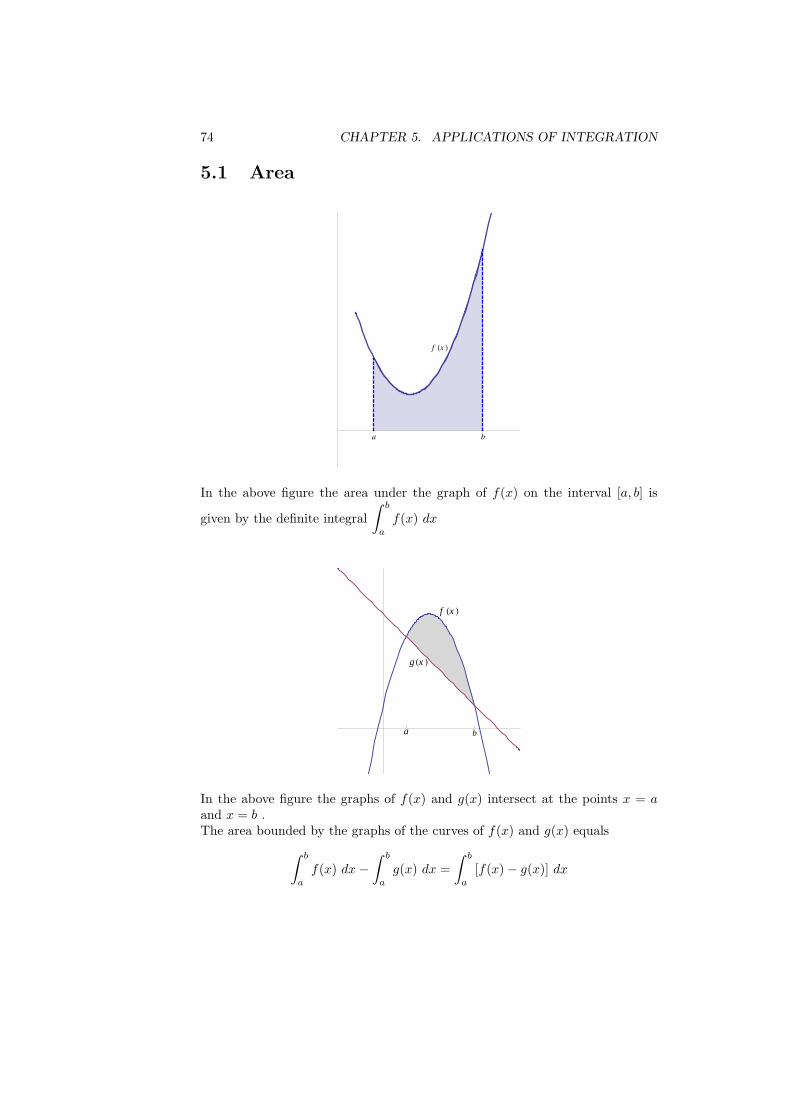
In the above figure the area under the graph of f(x) on the interval [a, b] is
given by the definite integral
∫ b
a
f(x) dx
f Hx L
g Hx L
a b
In the above figure the graphs of f(x) and g(x) intersect at the points x = a
and x = b .The area bounded by the graphs of the curves of f(x) and g(x) equals
∫ b
a
f(x) dx−∫ b
a
g(x) dx =
∫ b
a
[f(x)− g(x)] dx
5.1. AREA 75
Examples :
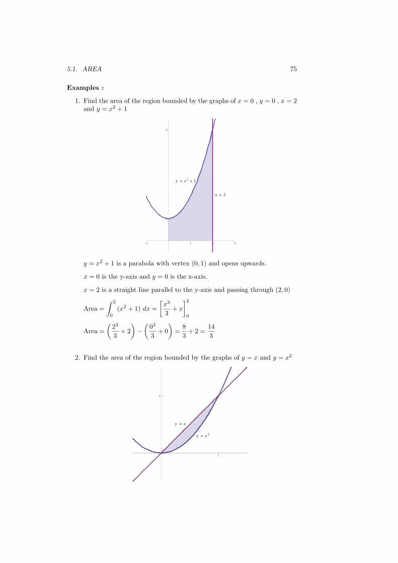
1. Find the area of the region bounded by the graphs of x = 0 , y = 0 , x = 2and y = x2 + 1
y = x 2+ 1
x = 2
-1 1 2 3
1
5
y = x2 + 1 is a parabola with vertex (0, 1) and opens upwards.
x = 0 is the y-axis and y = 0 is the x-axis.
x = 2 is a straight line parallel to the y-axis and passing through (2, 0)
Area =
∫ 2
0
(x2 + 1) dx =
[
x3
3+ x
]2
0
Area =
(
23
3+ 2
)
−(
03
3+ 0
)
=8
3+ 2 =
14
3
2. Find the area of the region bounded by the graphs of y = x and y = x2
y = x 2
y = x
1
1
76 CHAPTER 5. APPLICATIONS OF INTEGRATION
y = x2 is a parabola with vertex (0, 0) and opens upwards.
y = x is a straight line passing through the origin with slope equals 1.
Points of intersection of y = x2 and y = x :
x2 = x ⇒ x2 − x = 0 ⇒ x(x− 1) = 0 ⇒ x = 0 , x = 1
Area =
∫ 1
0
(x− x2) dx =
[
x2
2− x3
3
]1
0
Area =
(
12
2− 13
3
)
−(
02
2− 03
3
)
=1
2− 1
3=
1
6
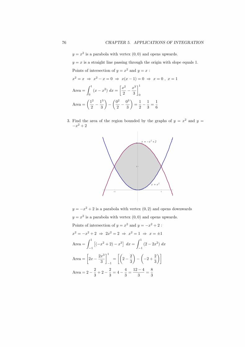
3. Find the area of the region bounded by the graphs of y = x2 and y =−x2 + 2
y = - x 2+ 2
y = x 2
-1 1
1
2
y = −x2 + 2 is a parabola with vertex (0, 2) and opens downwards
y = x2 is a parabola with vertex (0, 0) and opens upwards.
Points of intersection of y = x2 and y = −x2 + 2 :
x2 = −x2 + 2 ⇒ 2x2 = 2 ⇒ x2 = 1 ⇒ x = ±1
Area =
∫ 1
−1
[
(−x2 + 2)− x2]
dx =
∫ 1
−1
(2− 2x2) dx
Area =
[
2x− 2x3
3
]1
−1
=
[(
2− 2
3
)
−(
−2 +2
3
)]
Area = 2− 2
3+ 2− 2
3= 4− 4
3=
12− 4
3=
8
3
5.1. AREA 77
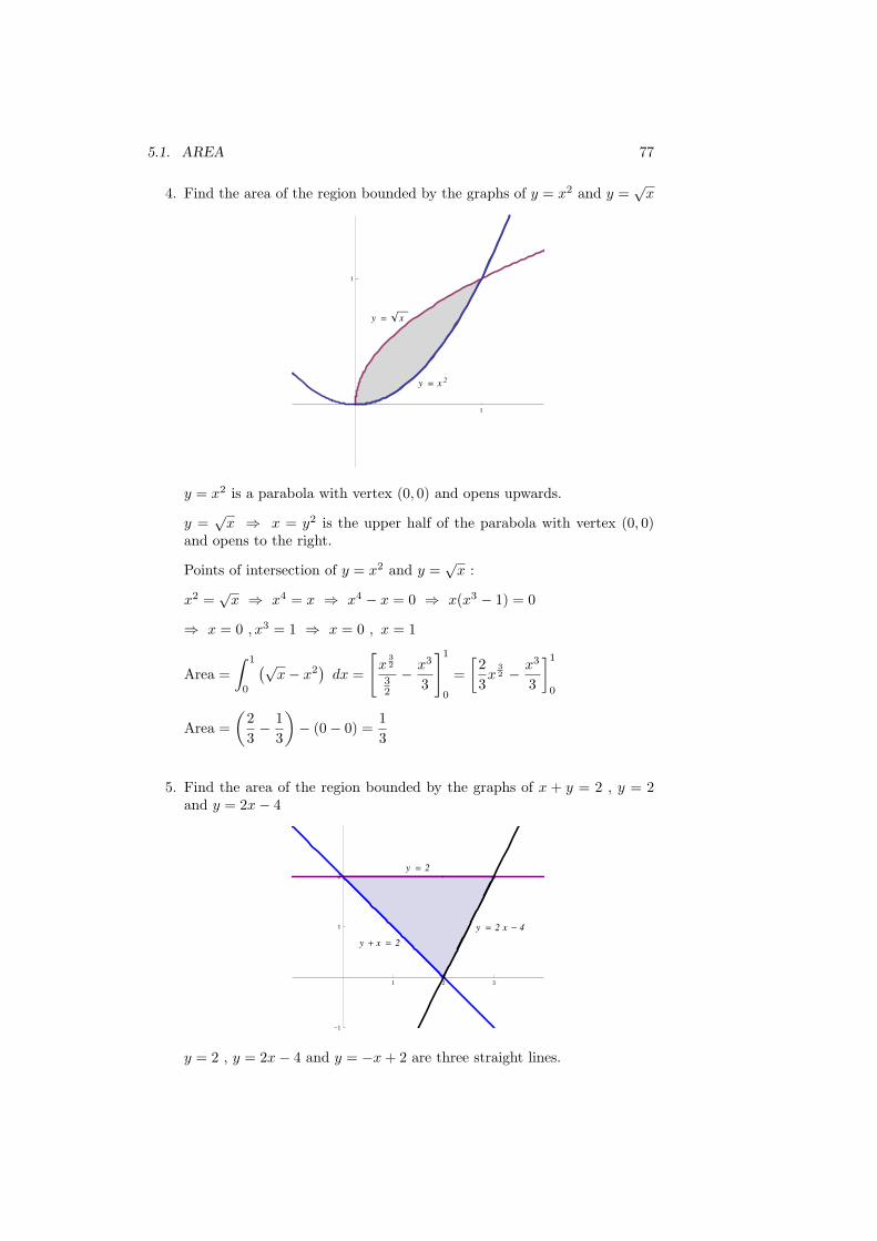
4. Find the area of the region bounded by the graphs of y = x2 and y =√x
y = x 2
y = x
1
1
y = x2 is a parabola with vertex (0, 0) and opens upwards.
y =√x ⇒ x = y2 is the upper half of the parabola with vertex (0, 0)
and opens to the right.
Points of intersection of y = x2 and y =√x :
x2 =√x ⇒ x4 = x ⇒ x4 − x = 0 ⇒ x(x3 − 1) = 0
⇒ x = 0 , x3 = 1 ⇒ x = 0 , x = 1
Area =
∫ 1
0
(√x− x2
)
dx =
[
x3
2
32
− x3
3
]1
0
=
[
2
3x
3
2 − x3
3
]1
0
Area =
(
2
3− 1
3
)
− (0− 0) =1
3
5. Find the area of the region bounded by the graphs of x + y = 2 , y = 2and y = 2x− 4
y = 2
y + x = 2
y = 2 x - 4
1 2 3
-1
1
2
y = 2 , y = 2x− 4 and y = −x+ 2 are three straight lines.
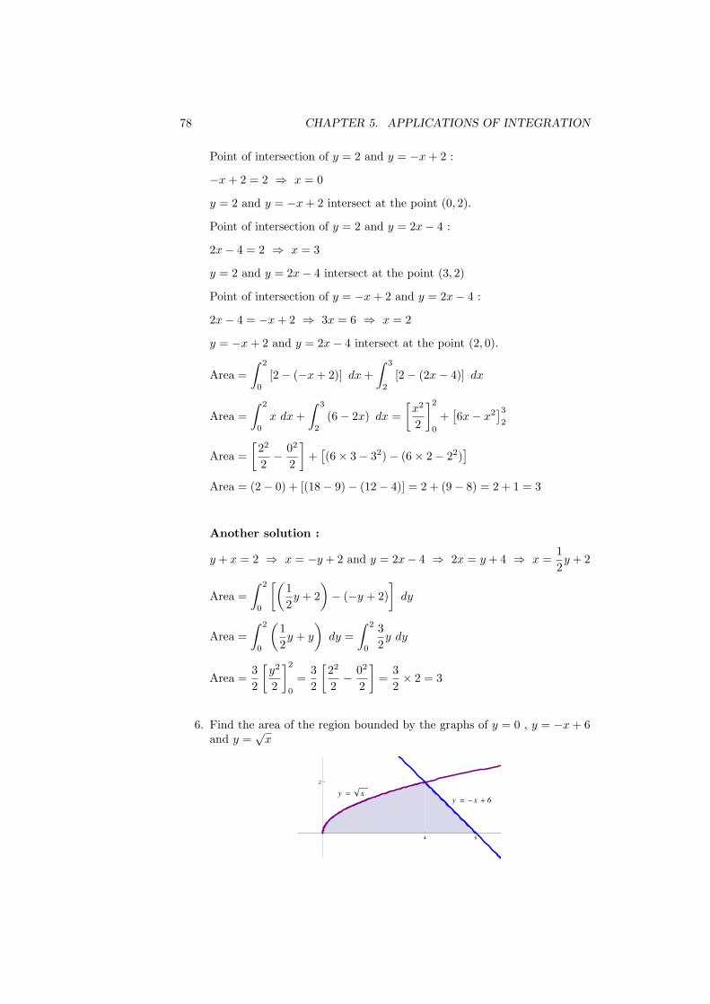
78 CHAPTER 5. APPLICATIONS OF INTEGRATION
Point of intersection of y = 2 and y = −x+ 2 :
−x+ 2 = 2 ⇒ x = 0
y = 2 and y = −x+ 2 intersect at the point (0, 2).
Point of intersection of y = 2 and y = 2x− 4 :
2x− 4 = 2 ⇒ x = 3
y = 2 and y = 2x− 4 intersect at the point (3, 2)
Point of intersection of y = −x+ 2 and y = 2x− 4 :
2x− 4 = −x+ 2 ⇒ 3x = 6 ⇒ x = 2
y = −x+ 2 and y = 2x− 4 intersect at the point (2, 0).
Area =
∫ 2
0
[2− (−x+ 2)] dx+
∫ 3
2
[2− (2x− 4)] dx
Area =
∫ 2
0
x dx+
∫ 3
2
(6− 2x) dx =
[
x2
2
]2
0
+[
6x− x2]3
2
Area =
[
22
2− 02
2
]
+[
(6× 3− 32)− (6× 2− 22)]
Area = (2− 0) + [(18− 9)− (12− 4)] = 2 + (9− 8) = 2 + 1 = 3
Another solution :
y + x = 2 ⇒ x = −y + 2 and y = 2x− 4 ⇒ 2x = y + 4 ⇒ x =1
2y + 2
Area =
∫ 2
0
[(
1
2y + 2
)
− (−y + 2)
]
dy
Area =
∫ 2
0
(
1
2y + y
)
dy =
∫ 2
0
3
2y dy
Area =3
2
[
y2
2
]2
0
=3
2
[
22
2− 02
2
]
=3
2× 2 = 3
6. Find the area of the region bounded by the graphs of y = 0 , y = −x+ 6and y =
√x
y = xy = - x + 6
4 6
2
5.1. AREA 79
y = −x+ 6 is a straight line passing through (0, 6) with slope equals −1.
y =√x ⇒ x = y2 is the upper half of the parabola with vertex (0, 0)
and opens to the right.
Points of intersection of x = y2 and x = −y + 6 :
y2 = −y+6 ⇒ y2 + y− 6 = 0 ⇒ (y− 2)(y+3) = 0 ⇒ y = 2 , y = −3
(Note that y = −3 is not in the desired region).
Area =
∫ 2
0
[
(−y + 6)− y2]
dy =
[
6y − y2
2− y3
3
]2
0
Area =
(
12− 4
2− 8
3
)
− (0−0−0) = 12−2− 8
3= 10− 8
3=
30− 8
3=
22
3
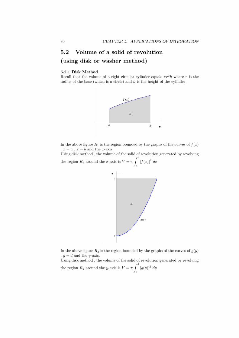
80 CHAPTER 5. APPLICATIONS OF INTEGRATION
5.2 Volume of a solid of revolution
(using disk or washer method)
5.2.1 Disk MethodRecall that the volume of a right circular cylinder equals πr2h where r is theradius of the base (which is a circle) and h is the height of the cylinder .
f Hx L
a b
R1
In the above figure R1 is the region bounded by the graphs of the curves of f(x), x = a , x = b and the x-axis.Using disk method , the volume of the solid of revolution generated by revolving
the region R1 around the x-axis is V = π
∫ b
a
[f(x)]2 dx
d
c
g Hy L
R2
In the above figure R2 is the region bounded by the graphs of the curves of g(y), y = d and the y-axis.Using disk method , the volume of the solid of revolution generated by revolving
the region R2 around the y-axis is V = π
∫ d
c
[g(y)]2 dy
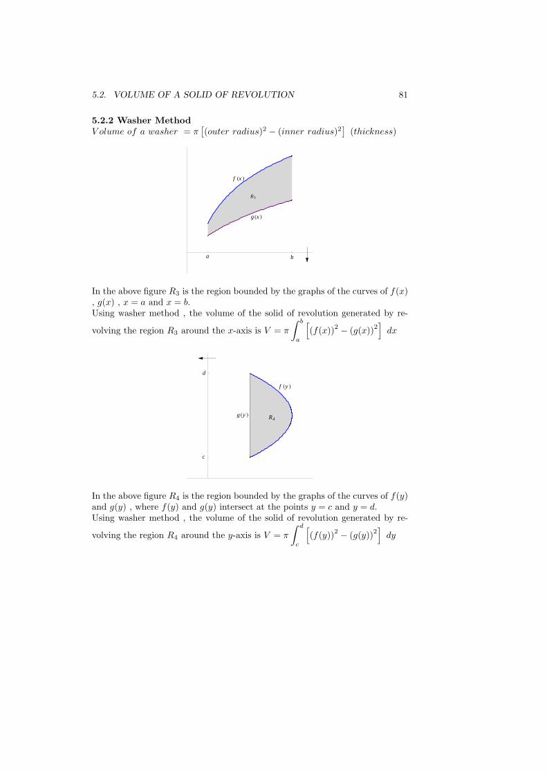
5.2. VOLUME OF A SOLID OF REVOLUTION 81
5.2.2 Washer MethodV olume of a washer = π
[
(outer radius)2 − (inner radius)2]
(thickness)
a b
g Hx L
f Hx L
R3
In the above figure R3 is the region bounded by the graphs of the curves of f(x), g(x) , x = a and x = b.Using washer method , the volume of the solid of revolution generated by re-
volving the region R3 around the x-axis is V = π
∫ b
a
[
(f(x))2 − (g(x))
2]
dx
c
d
f Hy L
g Hy L R4
In the above figure R4 is the region bounded by the graphs of the curves of f(y)and g(y) , where f(y) and g(y) intersect at the points y = c and y = d.Using washer method , the volume of the solid of revolution generated by re-
volving the region R4 around the y-axis is V = π
∫ d
c
[
(f(y))2 − (g(y))
2]
dy
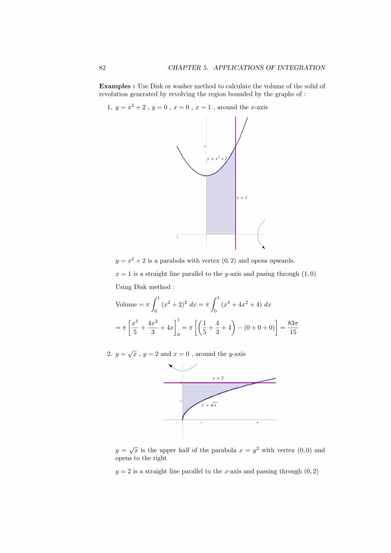
82 CHAPTER 5. APPLICATIONS OF INTEGRATION
Examples : Use Disk or washer method to calculate the volume of the solid ofrevolution generated by revolving the region bounded by the graphs of :
1. y = x2 + 2 , y = 0 , x = 0 , x = 1 , around the x-axis
x = 1
y = x 2+ 2
-1 1
2
3
y = x2 + 2 is a parabola with vertex (0, 2) and opens upwards.
x = 1 is a straight line parallel to the y-axis and pasing through (1, 0)
Using Disk method :
Volume = π
∫ 1
0
(x2 + 2)2 dx = π
∫ 1
0
(x4 + 4x2 + 4) dx
= π
[
x5
5+
4x3
3+ 4x
]1
0
= π
[(
1
5+
4
3+ 4
)
− (0 + 0 + 0)
]
=83π
15
2. y =√x , y = 2 and x = 0 , around the y-axis
y = 2
y = x
1 4
1
2
y =√x is the upper half of the parabola x = y2 with vertex (0, 0) and
opens to the right
y = 2 is a straight line parallel to the x-axis and passing through (0, 2)
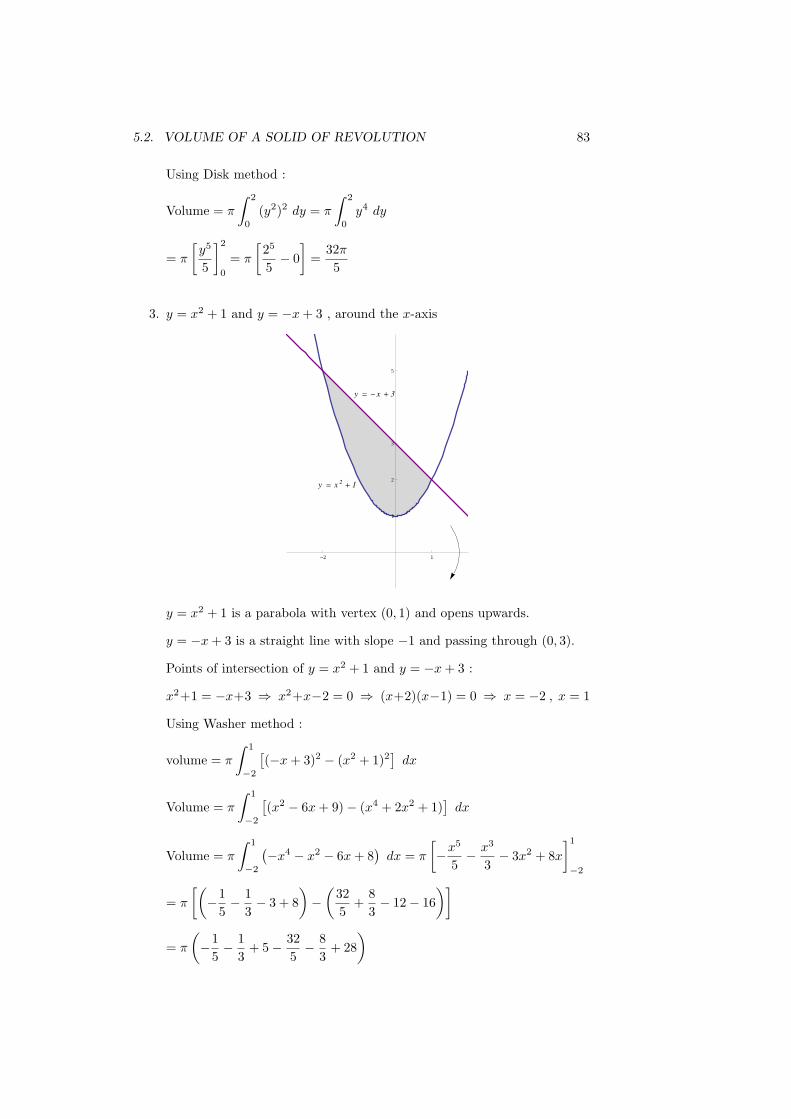
5.2. VOLUME OF A SOLID OF REVOLUTION 83
Using Disk method :
Volume = π
∫ 2
0
(y2)2 dy = π
∫ 2
0
y4 dy
= π
[
y5
5
]2
0
= π
[
25
5− 0
]
=32π
5
3. y = x2 + 1 and y = −x+ 3 , around the x-axis
y = - x + 3
y = x 2+ 1
-2 1
1
2
3
5
y = x2 + 1 is a parabola with vertex (0, 1) and opens upwards.
y = −x+ 3 is a straight line with slope −1 and passing through (0, 3).
Points of intersection of y = x2 + 1 and y = −x+ 3 :
x2+1 = −x+3 ⇒ x2+x−2 = 0 ⇒ (x+2)(x−1) = 0 ⇒ x = −2 , x = 1
Using Washer method :
volume = π
∫ 1
−2
[
(−x+ 3)2 − (x2 + 1)2]
dx
Volume = π
∫ 1
−2
[
(x2 − 6x+ 9)− (x4 + 2x2 + 1)]
dx
Volume = π
∫ 1
−2
(
−x4 − x2 − 6x+ 8)
dx = π
[
−x5
5− x3
3− 3x2 + 8x
]1
−2
= π
[(
−1
5− 1
3− 3 + 8
)
−(
32
5+
8
3− 12− 16
)]
= π
(
−1
5− 1
3+ 5− 32
5− 8
3+ 28
)
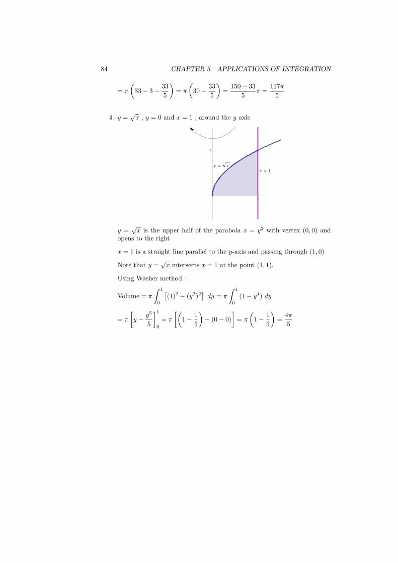
84 CHAPTER 5. APPLICATIONS OF INTEGRATION
= π
(
33− 3− 33
5
)
= π
(
30− 33
5
)
=150− 33
5π =
117π
5
4. y =√x , y = 0 and x = 1 , around the y-axis
x = 1
y = x
1
1
y =√x is the upper half of the parabola x = y2 with vertex (0, 0) and
opens to the right
x = 1 is a straight line parallel to the y-axis and passing through (1, 0)
Note that y =√x intersects x = 1 at the point (1, 1).
Using Washer method :
Volume = π
∫ 1
0
[
(1)2 − (y2)2]
dy = π
∫ 1
0
(1− y4) dy
= π
[
y − y5
5
]1
0
= π
[(
1− 1
5
)
− (0− 0)
]
= π
(
1− 1
5
)
=4π
5
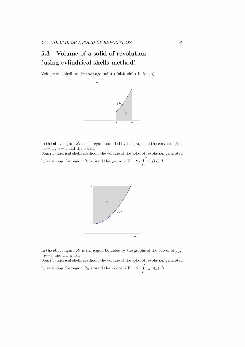
5.3. VOLUME OF A SOLID OF REVOLUTION 85
5.3 Volume of a solid of revolution
(using cylindrical shells method)
Volume of a shell = 2π (average radius) (altitude) (thickness)
a b
R1
f Hx L
In the above figure R1 is the region bounded by the graphs of the curves of f(x), x = a , x = b and the x-axis.Using cylindrical shells method , the volume of the solid of revolution generated
by revolving the region R1 around the y-axis is V = 2π
∫ b
a
x f(x) dx
c
d
g Hy L
R2
In the above figure R2 is the region bounded by the graphs of the curves of g(y), y = d and the y-axis.Using cylindrical shells method , the volume of the solid of revolution generated
by revolving the region R2 around the x-axis is V = 2π
∫ d
c
y g(y) dy
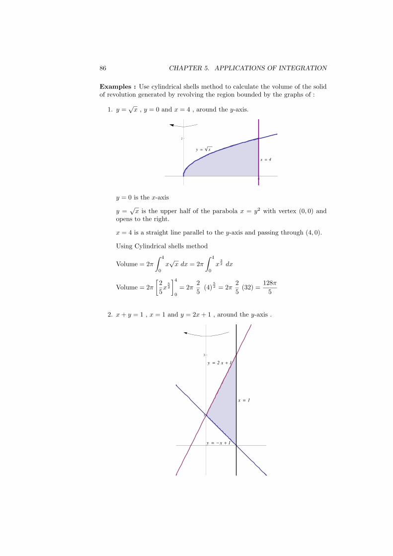
86 CHAPTER 5. APPLICATIONS OF INTEGRATION
Examples : Use cylindrical shells method to calculate the volume of the solidof revolution generated by revolving the region bounded by the graphs of :
1. y =√x , y = 0 and x = 4 , around the y-axis.
x = 4
y = x
4
2
y = 0 is the x-axis
y =√x is the upper half of the parabola x = y2 with vertex (0, 0) and
opens to the right.
x = 4 is a straight line parallel to the y-axis and passing through (4, 0).
Using Cylindrical shells method
Volume = 2π
∫ 4
0
x√x dx = 2π
∫ 4
0
x3
2 dx
Volume = 2π
[
2
5x
5
2
]4
0
= 2π2
5(4)
5
2 = 2π2
5(32) =
128π
5
2. x+ y = 1 , x = 1 and y = 2x+ 1 , around the y-axis .
y = - x + 1
y = 2 x + 1
x = 1
1
1
3
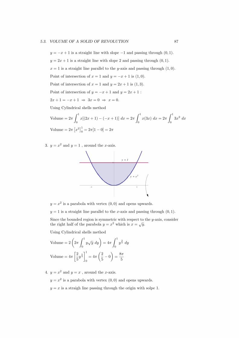
5.3. VOLUME OF A SOLID OF REVOLUTION 87
y = −x+ 1 is a straight line with slope −1 and passing through (0, 1).
y = 2x+ 1 is a straight line with slope 2 and passing through (0, 1).
x = 1 is a straight line parallel to the y-axis and passing through (1, 0).
Point of intersection of x = 1 and y = −x+ 1 is (1, 0).
Point of intersection of x = 1 and y = 2x+ 1 is (1, 3).
Point of intersection of y = −x+ 1 and y = 2x+ 1 :
2x+ 1 = −x+ 1 ⇒ 3x = 0 ⇒ x = 0.
Using Cylindrical shells method
Volume = 2π
∫ 1
0
x[(2x+ 1)− (−x+ 1)] dx = 2π
∫ 1
0
x(3x) dx = 2π
∫ 1
0
3x2 dx
Volume = 2π[
x3]1
0= 2π[1− 0] = 2π
3. y = x2 and y = 1 , around the x-axis.
y = 1
y = x 2
-1 1
1
y = x2 is a parabola with vertex (0, 0) and opens upwards.
y = 1 is a straight line parallel to the x-axis and passing through (0, 1).
Since the bounded region is symmetric with respect to the y-axis, considerthe right half of the parabola y = x2 which is x =
√y.
Using Cylindrical shells method
Volume = 2
(
2π
∫ 1
0
y√y dy
)
= 4π
∫ 1
0
y3
2 dy
Volume = 4π
[
2
5y
5
2
]1
0
= 4π
(
2
5− 0
)
=8π
5
4. y = x2 and y = x , around the x-axis.
y = x2 is a parabola with vertex (0, 0) and opens upwards.
y = x is a straigh line passing through the origin with solpe 1.
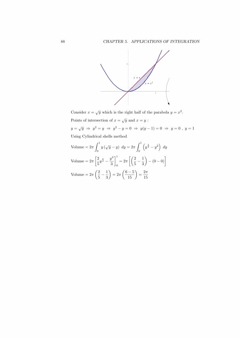
88 CHAPTER 5. APPLICATIONS OF INTEGRATION
y = x
y = x 2
1
1
Consider x =√y which is the right half of the parabola y = x2.
Points of intersection of x =√y and x = y :
y =√y ⇒ y2 = y ⇒ y2 − y = 0 ⇒ y(y − 1) = 0 ⇒ y = 0 , y = 1
Using Cylindrical shells method
Volume = 2π
∫ 1
0
y (√y − y) dy = 2π
∫ 1
0
(
y3
2 − y2)
dy
Volume = 2π
[
2
5y
5
2 − y3
3
]1
0
= 2π
[(
2
5− 1
3
)
− (0− 0)
]
Volume = 2π
(
2
5− 1
3
)
= 2π
(
6− 5
15
)
=2π
15
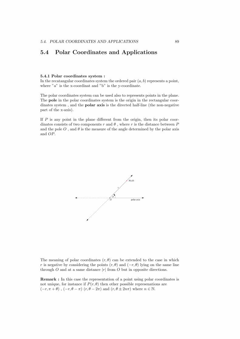
5.4. POLAR COORDINATES AND APPLICATIONS 89
5.4 Polar Coordinates and Applications
5.4.1 Polar coordinates system :In the recatangular coordinates system the ordered pair (a, b) represents a point,where ”a” is the x-coordinat and ”b” is the y-coordinate.
The polar coordinates system can be used also to represents points in the plane.The pole in the polar coordinates system is the origin in the rectangular coor-dinates system , and the polar axis is the directed half-line (the non-negativepart of the x-axis).
If P is any point in the plane different from the origin, then its polar coor-dinates consists of two components r and θ , where r is the distance between P
and the pole O , and θ is the measure of the angle determined by the polar axisand OP .
polar axisO
PHr,ΘL
Θ
r
The meaning of polar coordinates (r, θ) can be extended to the case in whichr is negative by considering the points (r, θ) and (−r, θ) lying on the same linethrough O and at a same distance |r| from O but in opposite directions.
Remark : In this case the representation of a point using polar coordinates isnot unique, for instance if P (r, θ) then other possible represenations are(−r, π + θ) , (−r, θ − π) (r, θ − 2π) and (r, θ ± 2nπ) where n ∈ N.
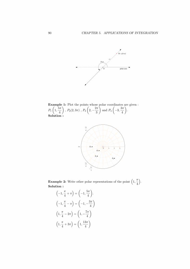
90 CHAPTER 5. APPLICATIONS OF INTEGRATION
polar axisO
PH-r,Θ+ΠL
Θ+Π
-r
Example 1: Plot the points whose polar coordinates are given :
P1
(
1,5π
4
)
, P2(2, 3π) , P3
(
2,−2π
3
)
and P4
(
−3,3π
4
)
.
Solution :
-
2 Π
3
3 Π
4
5 Π
4
3 Π0. 1. 2. 3.
P1
P2
P3
P4
Example 2: Write other polar reprsentations of the point(
1,π
4
)
.
Solution :(
−1,π
4+ π
)
=
(
−1,5π
4
)
.
(
−1,π
4− π
)
=
(
−1,−3π
4
)
(
1,π
4− 2π
)
=
(
1,−7π
4
)
(
1,π
4+ 3π
)
=
(
1,13π
4
)
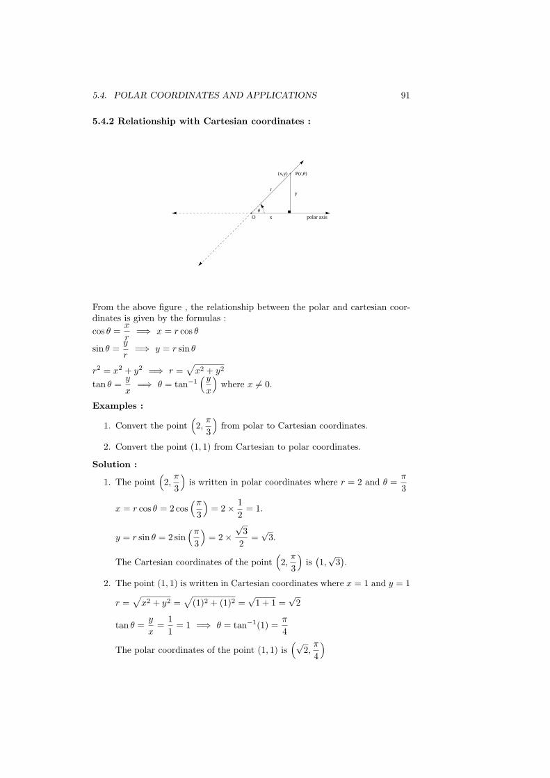
5.4. POLAR COORDINATES AND APPLICATIONS 91
5.4.2 Relationship with Cartesian coordinates :
polar axisO
PHr,ΘL
Θ
r
x
y
Hx,yL
From the above figure , the relationship between the polar and cartesian coor-dinates is given by the formulas :
cos θ =x
r=⇒ x = r cos θ
sin θ =y
r=⇒ y = r sin θ
r2 = x2 + y2 =⇒ r =√
x2 + y2
tan θ =y
x=⇒ θ = tan−1
(y
x
)
where x 6= 0.
Examples :
1. Convert the point(
2,π
3
)
from polar to Cartesian coordinates.
2. Convert the point (1, 1) from Cartesian to polar coordinates.
Solution :
1. The point(
2,π
3
)
is written in polar coordinates where r = 2 and θ =π
3
x = r cos θ = 2 cos(π
3
)
= 2× 1
2= 1.
y = r sin θ = 2 sin(π
3
)
= 2×√3
2=
√3.
The Cartesian coordinates of the point(
2,π
3
)
is(
1,√3)
.
2. The point (1, 1) is written in Cartesian coordinates where x = 1 and y = 1
r =√
x2 + y2 =√
(1)2 + (1)2 =√1 + 1 =
√2
tan θ =y
x=
1
1= 1 =⇒ θ = tan−1(1) =
π
4
The polar coordinates of the point (1, 1) is(√
2,π
4
)
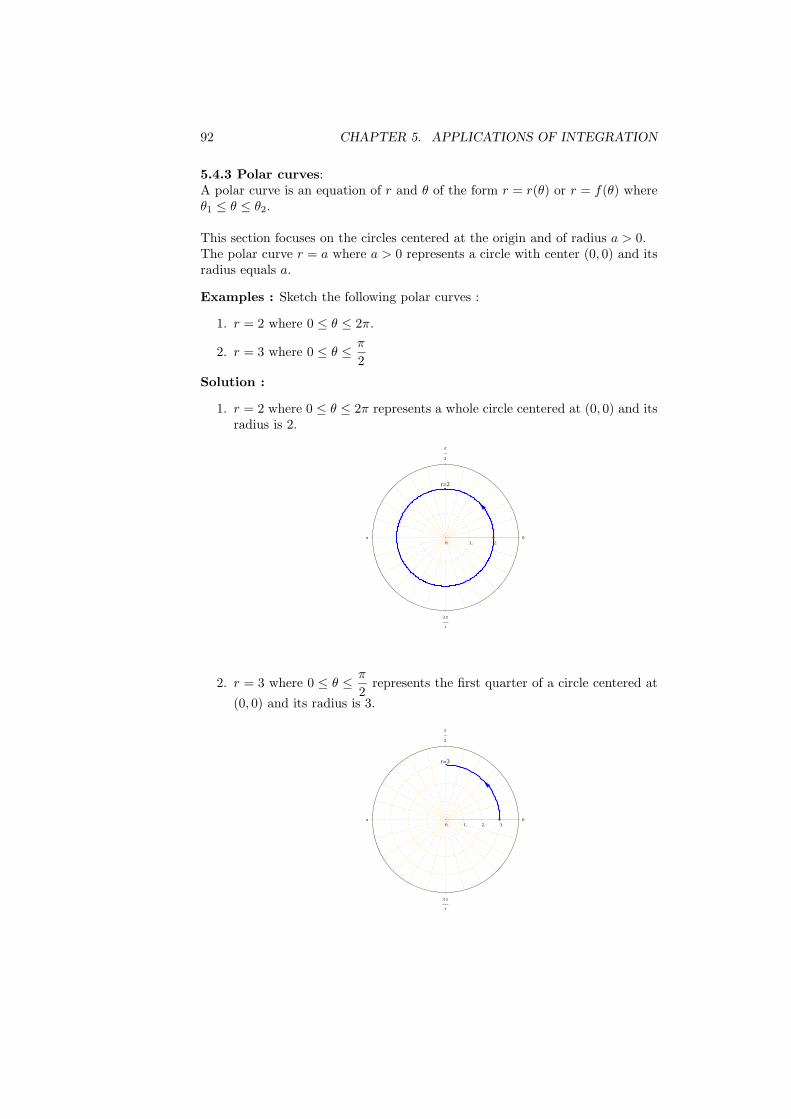
92 CHAPTER 5. APPLICATIONS OF INTEGRATION
5.4.3 Polar curves:A polar curve is an equation of r and θ of the form r = r(θ) or r = f(θ) whereθ1 ≤ θ ≤ θ2.
This section focuses on the circles centered at the origin and of radius a > 0.The polar curve r = a where a > 0 represents a circle with center (0, 0) and itsradius equals a.
Examples : Sketch the following polar curves :
1. r = 2 where 0 ≤ θ ≤ 2π.
2. r = 3 where 0 ≤ θ ≤ π
2
Solution :
1. r = 2 where 0 ≤ θ ≤ 2π represents a whole circle centered at (0, 0) and itsradius is 2.
0
Π
2
Π
3 Π
2
0. 1. 2.
r=2
2. r = 3 where 0 ≤ θ ≤ π
2represents the first quarter of a circle centered at
(0, 0) and its radius is 3.
0
Π
2
Π
3 Π
2
0. 1. 2. 3.
r=3
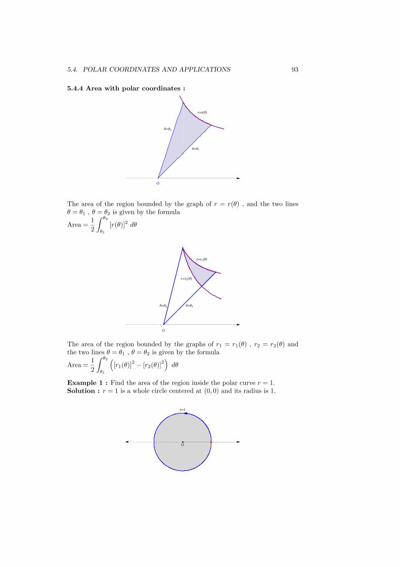
5.4. POLAR COORDINATES AND APPLICATIONS 93
5.4.4 Area with polar coordinates :
Θ=Θ1
r=rHΘL
Θ=Θ2
O
The area of the region bounded by the graph of r = r(θ) , and the two linesθ = θ1 , θ = θ2 is given by the formula
Area =1
2
∫ θ2
θ1
[r(θ)]2 dθ
Θ=Θ1
r=r1HΘL
r=r2HΘL
Θ=Θ2
O
The area of the region bounded by the graphs of r1 = r1(θ) , r2 = r2(θ) andthe two lines θ = θ1 , θ = θ2 is given by the formula
Area =1
2
∫ θ2
θ1
(
[r1(θ)]2 − [r2(θ)]
2)
dθ
Example 1 : Find the area of the region inside the polar curve r = 1.Solution : r = 1 is a whole circle centered at (0, 0) and its radius is 1.
O
r=1
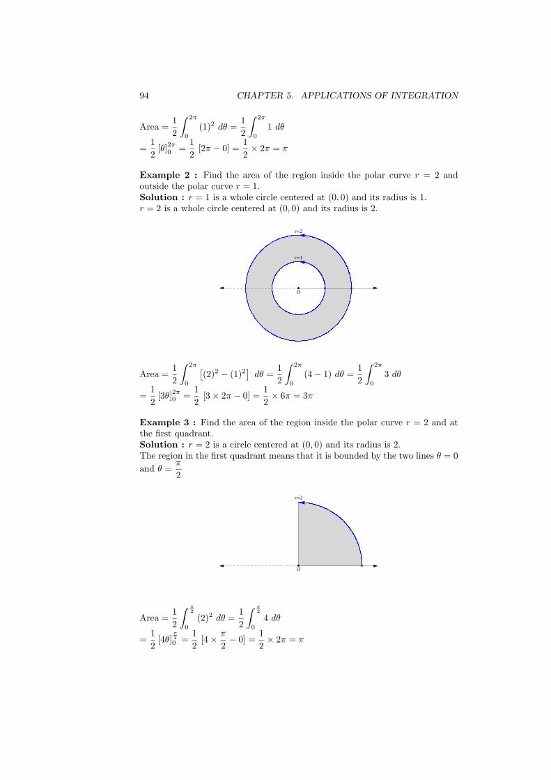
94 CHAPTER 5. APPLICATIONS OF INTEGRATION
Area =1
2
∫ 2π
0
(1)2 dθ =1
2
∫ 2π
0
1 dθ
=1
2[θ]
2π0 =
1
2[2π − 0] =
1
2× 2π = π
Example 2 : Find the area of the region inside the polar curve r = 2 andoutside the polar curve r = 1.Solution : r = 1 is a whole circle centered at (0, 0) and its radius is 1.r = 2 is a whole circle centered at (0, 0) and its radius is 2.
O
r=1
r=2
Area =1
2
∫ 2π
0
[
(2)2 − (1)2]
dθ =1
2
∫ 2π
0
(4− 1) dθ =1
2
∫ 2π
0
3 dθ
=1
2[3θ]
2π0 =
1
2[3× 2π − 0] =
1
2× 6π = 3π
Example 3 : Find the area of the region inside the polar curve r = 2 and atthe first quadrant.Solution : r = 2 is a circle centered at (0, 0) and its radius is 2.The region in the first quadrant means that it is bounded by the two lines θ = 0
and θ =π
2
O
r=2
Area =1
2
∫ π
2
0
(2)2 dθ =1
2
∫ π
2
0
4 dθ
=1
2[4θ]
π
2
0 =1
2[4× π
2− 0] =
1
2× 2π = π
Chapter 6
PARTIAL DERIVATIVES
6.1 Functions of several variables
6.2 Partial derivatives
6.3 Chain Rules
6.4 Implicit differentiation
95
96 CHAPTER 6. PARTIAL DERIVATIVES
6.1 Functions of several variables
6.1.1 Functions of two variables :Definition: A function of two variables is a rule that assigns an ordered pair(x, y) (in the domain of the function) to a real number w.
f : R2 −→ R
(x, y) −→ w
Example :
f(x, y) =y
x2 + y2is a function of two variables x and y
f(3, 1) =1
32 + 12=
1
10.
Note that f(x, y) takes (3, 1) ∈ R2 to
1
10∈ R
6.1.2 Functions of three variables :Definition: A function of three variables is a rule that assigns an ordered triple(x, y, z) (in the domain of the function) to a real number w .
f : R3 −→ R
(x, y, z) −→ w
Example :
f(x, y, z) =z
x+ y2 + 3is a function of three variables x , y and z
f(1,−2, 4) =4
1 + (−2)2 + 3=
4
8=
1
2.
Note that f(x, y, z) takes (1,−2, 4) ∈ R3 to
1
2∈ R
6.2. PARTIAL DERIVATIVES 97
6.2 Partial derivatives
6.2.1 Partial derivatives of a function of two variables :If w = f(x, y) is a function of two variables, then :
1. The partial derivative of f with respect to x is denoted by∂f
∂x,∂w
∂x, fx
or wx , and it is calculated by applying the rules of differentiation to x
and regarding y as a constant .
2. The partial derivative of f with respect to y is denoted by∂f
∂y,∂w
∂y, fy
or wy , and it is calculated by applying the rules of differentiation to y
and regarding x as a constant .
Example 1: Calculate fx and fy of the functiuon f(x, y) = x2y3+xy ln(x+ y)Solution:
1. fx =∂
∂x
(
x2y3 + xy ln(x+ y))
fx = (2x)y3 +
[
(1)y ln(x+ y) + xy1
x+ y
]
= 2xy3 + y ln(x+ y) +xy
x+ y
2. fy =∂
∂y
(
x2y3 + xy ln(x+ y))
fy = x2(3y2) +
[
x(1) ln(x+ y) + xy1
x+ y
]
= 3x2y2 + x ln(x+ y) +xy
x+ y
Example 2: Calculate fx and fy of the functiuon f(x, y) =x+ y2
x+ ySolution:
1. fx =∂f
∂x=
(1 + 0)(x+ y)− (x+ y2)(1 + 0)
(x+ y)2=
x+ y − (x+ y2)
(x+ y2)
fx =x+ y − x− y2
(x+ y)2=
y − y2
(x+ y)2
2. fy =∂f
∂y=
(0 + 2y)(x+ y)− (x+ y2)(0 + 1)
(x+ y)2=
2y(x+ y)− (x+ y2)
(x+ y)2
fy =2xy + 2y2 − x− y2
(x+ y)2=
2xy − x+ y2
(x+ y)2
98 CHAPTER 6. PARTIAL DERIVATIVES
6.2.2 Partial derivatives of a function of three variables :If w = f(x, y, z) is a function of three variables, then :
1. The partial derivative of f with respect to x is denoted by∂f
∂x,∂w
∂x, fx
or wx , and it is calculated by applying the rules of differentiation to x
and regarding y and z as constants .
2. The partial derivative of f with respect to y is denoted by∂f
∂y,∂w
∂y, fy
or wy , and it is calculated by applying the rules of differentiation to y
and regarding x and z as constants .
3. The partial derivative of f with respect to z is denoted by∂f
∂z,∂w
∂z, fz
or wz , and it is calculated by applying the rules of differentiation to z
and regarding x and y as constants .
Example : If f(x, y, z) = 2z3x− 4(x2 + y2)z , then calculate fx , fy and fz at(0, 1, 2).Solution :
1. fx =∂
∂x
(
2z3x− 4(x2 + y2)z)
= 2z3 − 4(2x)z = 2z3 − 8xz
fx(0, 1, 2) = 2 (23)− 8(0)(2) = 16
2. fy =∂
∂y
(
2z3x− 4(x2 + y2)z)
= 0− 4(0 + 2y)z = −8yz
fy(0, 1, 2) = −8(1)(2) = −16
3. fz =∂
∂z
(
2z3x− 4(x2 + y2)z)
= 6z2x− 4(x2 + y2)
fz(0, 1, 2) = 6(22)(0)− 4(02 + 12) = −4
6.2.3 Second partial derivatives :If w = f(x, y) is a function of two variables , then :
1.∂2f
∂x2=
∂
∂x
(
∂f
∂x
)
=∂
∂x(fx) = fxx .
2.∂2f
∂y2=
∂
∂y
(
∂f
∂y
)
=∂
∂y(fy) = fyy .
3.∂2f
∂x∂y=
∂
∂x
(
∂f
∂y
)
=∂
∂x(fy) = fyx .
4.∂2f
∂y∂x=
∂
∂y
(
∂f
∂x
)
=∂
∂y(fx) = fxy .
6.2. PARTIAL DERIVATIVES 99
Note : Second partial derivatives of a function of three variables are defined ina same manner.
Theorem : Let f(x, y) be a function of two variables. If f , fx , fy , fxy andfyx are continuous, then fxy = fyx.
Note : If f(x, y, z) is a function of three variables and f has continuous secondpartial derivatives, then fxy = fyx , fxz = fzx and fyz = fzy .
Example 1: Let f(x, y) = x3y + xy2 sin(x+ y) , calculate∂2f
∂x∂yand
∂2f
∂y∂xSolution :
fx = 3x2y + y2 sin(x+ y) + xy2 cos(x+ y)
fy = x3 + 2xy sin(x+ y) + xy2 cos(x+ y)
fxy = 3x2 +2y sin(x+ y) + y2 cos(x+ y) + 2xy cos(x+ y)− xy2 sin(x+ y)
fyx = 3x2 +2y sin(x+ y) + 2xy cos(x+ y) + y2 cos(x+ y)− xy2 sin(x+ y)
Note : fxy = fyx according to the theorem .
Example 2: Let f(x, y, z) = x3y2z + xy sin(y+ z) , calculate∂2f
∂y∂xand
∂2f
∂x∂zSolution :
fx = 3x2y2z + y sin(y + z)
fz = x3y2 + xy cos(y + z)
∂2f
∂y∂x= fxy = 6x2yz + sin(y + z) + y cos(y + z)
∂2f
∂x∂z= fzx = 3x2y2 + y cos(y + z)
Example 3: Let f(x, y, z) = 2z3−3(x2+y2)z , Show that∂2f
∂x2+∂2f
∂y2+∂2f
∂z2= 0
Solution :
fx = 0− 3z(2x) = −6xz
fy = 0− 3z(2y) = −6yz
fz = 6z2 − 3(x2 + y2)
∂2f
∂x2= fxx = −6z
∂2f
∂y2= fyy = −6z
100 CHAPTER 6. PARTIAL DERIVATIVES
∂2f
∂z2= fzz = 12z
∂2f
∂x2+
∂2f
∂y2+
∂2f
∂z2= −6z − 6z + 12z = 0
6.3. CHAIN RULES 101
6.3 Chain Rules
Theorem (Chain Rules):
1. If w = f(x, y) and x = g(t) , y = h(t) , such that f , g and h aredifferentiable then
df
dt=
dw
dt=
∂w
∂x
dx
dt+
∂w
∂y
dy
dt
2. If w = f(x, y) and x = g(t, s) , y = h(t, s) , such that f , g and h aredifferentiable then
∂f
∂t=
∂w
∂t=
∂w
∂x
∂x
∂t+
∂w
∂y
∂y
∂t
∂f
∂s=
∂w
∂s=
∂w
∂x
∂x
∂s+
∂w
∂y
∂y
∂s
3. If w = f(x, y, z) and x = g(t, s) , y = h(t, s) , z = k(t, s) such that f , g ,h and k are differentiable then
∂w
∂t=
∂w
∂x
∂x
∂t+
∂w
∂y
∂y
∂t+
∂w
∂z
∂z
∂t
∂w
∂s=
∂w
∂x
∂x
∂s+
∂w
∂y
∂y
∂s+
∂w
∂z
∂z
∂s
Example 1 : Let f(x, y) = xy + y2 , x = s2t , and y = s + t , calculate∂f
∂s
and∂f
∂t.
Solution :
1.∂f
∂s=
∂f
∂x
∂x
∂s+
∂f
∂y
∂y
∂s
∂f
∂x= y ,
∂x
∂s= 2st
∂f
∂y= x+ 2y ,
∂y
∂s= 1
∂f
∂s= y (2st) + (x+ 2y)(1) = (s+ t)2st+
[
s2t+ 2(s+ t)]
= 2s2t+ 2st2 + s2t+ 2s+ 2t = 3s2t+ 2st2 + 2s+ 2t
2.∂f
∂t=
∂f
∂x
∂x
∂t+
∂f
∂y
∂y
∂t
∂f
∂x= y ,
∂x
∂t= s2
∂f
∂y= x+ 2y ,
∂y
∂t= 1
102 CHAPTER 6. PARTIAL DERIVATIVES
∂f
∂t= ys2 + (x+ 2y)(1) = (s+ t)s2 + s2t+ 2(s+ t)
= s3 + s2t+ s2t+ 2s+ 2t = s3 + 2s2t+ 2s+ 2t
Example 2 : Let f(x, y, z) = x + sin(xy) + cos(xz) , x = ts , y = s + t and
z =s
t, calculate
∂f
∂sand
∂f
∂t.
Solution :
1.∂f
∂s=
∂f
∂x
∂x
∂s+
∂f
∂y
∂y
∂s+
∂f
∂z
∂z
∂s
∂f
∂x= 1 + y cos(xy)− z sin(xz) ,
∂x
∂s= t
∂f
∂y= x cos(xy) ,
∂y
∂s= 1
∂f
∂z= −x sin(xz) ,
∂z
∂s=
1
t
∂f
∂s= t [1 + y cos(xy)− z sin(xz)] + x cos(xy) +
(
1
t
)
(−x sin(xz))
∂f
∂s= t+ ty cos(xy)− tz sin(xz) + x cos(xy)− x sin(xz)
t
2.∂f
∂t=
∂f
∂x
∂x
∂t+
∂f
∂y
∂y
∂t+
∂f
∂z
∂z
∂t
∂f
∂x= 1 + y cos(xy)− z sin(xz) ,
∂x
∂t= s
∂f
∂y= x cos(xy) ,
∂y
∂t= 1
∂f
∂z= −x sin(xz) ,
∂z
∂t=
−s
t2
∂f
∂t= s [1 + y cos(xy)− z sin(xz)] + x cos(xy) +
(−s
t2
)
(−x sin(xz))
∂f
∂t= s+ sy cos(xy)− sz sin(xz) + x cos(xy) +
sx sin(xz)
t2
6.4. IMPLICIT DIFFERENTIATION 103
6.4 Implicit differentiation
1. Suppose that the equation F (x, y) = 0 defines y implicitly as a functionof x say y = f(x) , then
dy
dx= −Fx
Fy
2. Suppose that the equation F (x, y, z) = 0 implicitly defines a functionz = f(x, y) , where f is differentiable , then
∂z
∂x= −Fx
Fz
and∂z
∂y= −Fy
Fz
Example 1 : Let y2 − xy + 3x2 = 0 , finddy
dx.
Solution 1: Let F (x, y) = x2 − xy + 3x2 then F (x, y) = 0
Fx = −y + 6x and Fy = 2y − x .
dy
dx= −Fx
Fy
= − (−y + 6x)
2y − x=
y − 6x
2y − x.
Solution 2 : y2 − xy + 3x2 = 0
Differentiate both sides implicitly
2yy′ − (y + xy′) + 6x = 0 ⇒ 2yy′ − y − xy′ + 6x = 0
⇒ 2yy′ − xy′ = y − 6x ⇒ (2y − x)y′ = y − 6x
⇒ dy
dx= y′ =
y − 6x
2y − x
Example 2 : Let F (x, y, z) = x2y + z2 + sin(xyz) = 0 , find∂z
∂xand
∂z
∂y.
Solution :
Fx = 2xy + yz cos(xyz)
Fy = x2 + xz cos(xyz)
Fz = 2z + xy cos(xyz)
∂z
∂x= −Fx
Fz
= −2xy + yz cos(xyz)
2z + xy cos(xyz)
∂z
∂y= −Fy
Fz
= −x2 + xz cos(xyz)
2z + xy cos(xyz)
104 CHAPTER 6. PARTIAL DERIVATIVES
Chapter 7
DIFFERENTIALEQUATIONS
7.1 Definition of a differential equation
7.2 Separable Differential equations
7.3 First-order linear differential equations
105
106 CHAPTER 7. DIFFERENTIAL EQUATIONS
7.1 Definition of a differential equation
Definition : An equation that involves x , y , y′ , y′′ , · · · , y(n) for a functiony(x) with nth derivative y(n) of y with respect to x is an ordinary differentialEquation of order n.
Examples :
1. y′ = x2 + 5 is a differential equation of order 1.
2. y′′ + x (y′)4 − y = x is a differential equation of order 2
3.(
y(4))3
+ x2 y′′ = 2x is a differnetial equation of order 4
y = y(x) is called a solution of a differential equation if y = y(x) satisfies thatdifferential equation.Consider the differential equation y′ = 6x + 4 , then y = 3x2 + 4x + c is thegeneral solution of that differential equation.
If an initial condition was added to the differential equation to assign a certainvallue for c then y = y(x) is called the particular solution of the differentialequation .Consider the differential equation y′ = 6x+4 with the initial condition y(0) = 2,y = 3x2 + 4x+ c is the general solution of the differential equation ,y(0) = 2 ⇒ 3(0)2 + 4 × 0 + c = 2 ⇒ c = 2 , hence y = 3x2 + 4x + 2 is theparticular solution of the differential equation.
7.2. SEPARABLE DIFFERENTIAL EQUATIONS 107
7.2 Separable Differential equations
The separable differential equation has the form M(x) +N(y) y′ = 0 .where M(x) and N(y) are continuous functions.
To solve the separable differential equation :
1. Write it as M(x) dx+N(y) dy = 0 =⇒ N(y) dy = −M(x) dx .
2. Integrate the left-hand side with respect to y and the right-hand side withrespect to x∫
N(y) dy = −∫
M(x) dx
Example 1 : Solve the differential equation y′ + y3ex = 0 .Solution :
y′ + y3ex = 0 =⇒ dy
dx= −y3ex ,
=⇒ − 1
y3dy = ex dx =⇒ − y−3 dy = ex dx
=⇒ −∫
y−3 dy =
∫
ex dx =⇒ − y−2
−2= ex + c
=⇒ 1
2y2= ex + c =⇒ 1
y2= 2 (ex + c)
=⇒ y2 =1
2 (ex + c)=⇒ y =
√
1
2 (ex + c)
Example 2 : Solve the differential equationdy
dx= y2ex , y(0) = 1.
Solution :
dy
dx= y2ex =⇒ 1
y2dy = ex dx
=⇒ y−2 dy = ex dx =⇒∫
y−2 dy =
∫
ex dx
=⇒ y−1
−1= ex + c =⇒ y =
−1
ex + c
Using the initial condition y(0) = 1 =⇒ 1 =−1
e0 + c
=⇒ 1 =−1
1 + c=⇒ 1 + c = −1 =⇒ c = −2
The particular solution is y =−1
ex − 2
108 CHAPTER 7. DIFFERENTIAL EQUATIONS
Example 3 : Solve the differential equation dy − sinx(1 + y2)dx = 0 .Solution :
dy − sinx(1 + y2)dx = 0 =⇒ dy = sinx(1 + y2)dx
=⇒ 1
1 + y2dy = sinx dx =⇒
∫
1
1 + y2dy =
∫
sinx dx
=⇒ tan−1 y = − cosx+ c =⇒ y = tan(− cosx+ c)
Example 4 : Solve the differential equation e−y sinx− y′ cos2 x = 0 .Solution :
e−y sinx− y′ cos2 x = 0 =⇒ − cos2 xdy
dx= −e−y sinx
=⇒ 1
e−ydy =
− sinx
− cos2 xdx =⇒ ey dy =
1
cosx
sinx
cosxdx
=⇒ ey dy = secx tanx dx =⇒∫
ey dy =
∫
secx tanx dx
=⇒ ey = secx+ c =⇒ y = ln | secx+ c|
Example 5 : Solve the differential equation y′ = 1− y + x2 − yx2 .Solution :
y′ = 1− y + x2 − yx2 =⇒ dy
dx= 1− y + x2(1− y)
=⇒ dy
dx= (1− y)(1 + x2) =⇒ 1
1− ydy = (1 + x2) dx
=⇒∫
1
1− ydy =
∫
(1 + x2) dx =⇒ −∫ −1
1− ydy =
∫
(1 + x2) dx
=⇒ − ln |1− y| = x+x3
3+ c =⇒ ln |1− y| = −x− x3
3− c
=⇒ 1− y = e−x−x3
3−c =⇒ y = 1− e−x−
x3
3−c
7.3. FIRST-ORDER LINEAR DIFFERENTIAL EQUATIONS 109
7.3 First-order linear differential equations
The first-order linear differential equation has the form y′ + P (x) y = Q(x) ,where P (x) and Q(x) are continuous functions of x
To solve the first-order linear differential equation :
1. Compute the integrating factor u(x) = e∫P (x) dx
2. The general solution of the first-order linear differential equation is
y(x) =1
u(x)
∫
u(x) Q(x) dx
Example 1 : Solve the differential equation xdy
dx+ y = x2 + 1 .
Solution :
xdy
dx+ y = x2 + 1 =⇒ y′ +
(
1
x
)
y =x2 + 1
x
=⇒ y′ +
(
1
x
)
y = x+1
x
P (x) =1
xand Q(x) = x+
1
x
The integrating factor is u(x) = e∫
1
xdx = eln x = x
The general solution is y =1
x
∫
x
(
x+1
x
)
dx
y =1
x
∫
(x2 + 1) dx =1
x
(
x3
3+ x+ c
)
=x2
3+ 1 +
c
x
Example 2 : Solve the differential equation y′ − 2
xy = x2ex , y(1) = e .
Solution :
P (x) = − 2
xand Q(x) = x2ex
The integrating factor is
u(x) = e∫−
2
xdx = e−2
∫1
xdx = e−2 ln x = eln x−2
= x−2
The general solution is y =1
x−2
∫
x−2x2exdx
y = x2
∫
exdx = x2(ex + c) = x2ex + cx2
Using the initial condition y(1) = e
110 CHAPTER 7. DIFFERENTIAL EQUATIONS
y(1) = e =⇒ e = (1)2e1 + c (1)2 =⇒ e = e+ c =⇒ c = 0
The particular solution is y = x2ex
Example 3 : Solve the differential equation y′ + y = cos(ex)Solution :
P (x) = 1 and Q(x) = cos(ex)
The integrating factor is u(x) = e∫1 dx = ex
The general solution is y =1
ex
∫
ex cos(ex) dx
y = e−x∫
cos(ex)ex dx = e−x (sin(ex) + c) = e−x sin(ex) + ce−x
Example 4 : Solve the differential equation xy′ − 3y = x2
Solution :
xy′ − 3y = x2 =⇒ y′ − 3
xy = x
P (x) = − 3
xand Q(x) = x
The integrating factor is
u(x) = e∫−
3
xdx = e−3
∫1
xdx = e−3 ln x = eln x−3
= x−3
The general solution is y =1
x−3
∫
x−3x dx
y = x3
∫
x−2dx = x3
(
x−1
−1+ c
)
y = x3
(
− 1
x+ c
)
= −x2 + cx3