Contentslyu/book/sft/pdf/chap5.pdf · Contents 5 Dependability ... 5.2 SYSTEM DESCRIPTIONS ... architectures (DRB, NVP, and NSCP) being considered in this chapter. The systems are

Contents

5 Dependability Modeling for Fault-Tolerant Software and Systems 1095.1 INTRODUCTION . . . . . . . . . . . . . . . . . . . . . . . . . . . . . . . 1095.2 SYSTEM DESCRIPTIONS . . . . . . . . . . . . . . . . . . . . . . . . . . 1105.3 MODELING ASSUMPTIONS AND PARAMETER DEFINITIONS . . . . . 1125.4 SYSTEM LEVEL MODELING . . . . . . . . . . . . . . . . . . . . . . . . 1145.5 EXPERIMENTAL DATA ANALYSIS . . . . . . . . . . . . . . . . . . . . . 1195.6 A CASE STUDY IN PARAMETER ESTIMATION . . . . . . . . . . . . . . 1245.7 QUANTITATIVE SYSTEM-LEVEL ANALYSIS . . . . . . . . . . . . . . . 1285.8 SENSITIVITY ANALYSIS . . . . . . . . . . . . . . . . . . . . . . . . . . . 1325.9 DECIDER FAILURE PROBABILITY . . . . . . . . . . . . . . . . . . . . . 1345.10 CONCLUSIONS . . . . . . . . . . . . . . . . . . . . . . . . . . . . . . . . 136

vi CONTENTS

5

Dependability Modeling forFault-Tolerant Software andSystemsJOANNE BECHTA DUGAN

University of Virginia

MICHAEL R. LYU

Bell Communications Research

ABSTRACT

Three major fault-tolerant software system architectures, distributed recovery blocks,N -version programming, and N self-checking programming, are modeled by a combinationof fault tree techniques and Markov processes. In these three architectures, transient andpermanent hardware faults as well as unrelated and related software faults are modeled inthe system-level domain. The model parameter values are determined from the analysis ofdata collected from a fault-tolerant avionic application. Quantitative analyses for reliabilityand safety factors achieved in these three fault-tolerant system architectures are presented.

5.1 INTRODUCTION

The complexity and size of current and future software systems, usually embedded in a sophis-ticated hardware architecture, are growing dramatically. As our requirements for and depen-dencies on computers and their operating software increase, the crises of computer hardware

Software Fault Tolerance, Edited by Lyuc© 1995 John Wiley & Sons Ltd

110 DUGAN and LYU

and failure failures also increase. The impact of computer failures to human life ranges frominconvenience (e.g., malfunctions of home appliances), economic loss (e.g., interceptions ofbanking systems) to life-threatening (e.g., failures of flight systems or nuclear reactors). Asthe faults in computer systems are unavoidable as the system complexity grows, computer sys-tems used for critical applications are designed to tolerate both software and hardware faultsby the configuration of multiple software versions on redundant hardware systems. Many suchapplications exist in the aerospace industry [Car84, You84, Hil85, Tra88], nuclear power in-dustry [Ram81, Bis86, Vog88], and ground transportation industry [Gun88].

The system architectures incorporating both hardware and software fault tolerance are ex-plored in three typical approaches. The distributed recovery blocks (DRB) scheme [Kim89]combines both distributed processing and recovery block (RB) [Ran75] concepts to providea unified approach to tolerating both hardware and software faults. Architectural considera-tions for the support ofN -version programming (NVP) [Avi85] were addressed in [Lal88], inwhich the FTP-AP system is described. The FTP-AP system achieves hardware and softwaredesign diversity by attaching application processors (AP) to the byzantine resilient hard coreFault Tolerant Processor (FTP). N self-checking programming (NSCP) [Lap90] uses diversehardware and software in self-checking groups to detect hardware and software induced errorsand forms the basis of the flight control system used on the Airbus A310 and A320 aircraft[Bri93].

Sophisticated techniques exist for the separate analysis of fault tolerant hardware [Gei90,Joh88] and software [Grn80, Shi84, Sco87, Cia92], but only some authors have consideredtheir combined analysis [Lap84, Sta87, Lap92]. This chapter uses a combination of fault treeand Markov modeling as a framework for the analysis of hardware and software fault tolerantsystems. The overall system model is a Markov model in which the states of the Markovchain represent the evolution of the hardware configuration as permanent faults occur and arehandled. A fault tree model captures the effects of software faults and transient hardware faultson the computation process. This hierarchical approach simplifies the development, solutionand understanding of the modeling process. We parameterize the values of each model bya recent fault-tolerant software project [Lyu93] to perform reliability and safety analysis ofeach architecture.

The chapter is organized as follows. In Section 5.2 we give a description of the three systemarchitectures studied in this chapter. Section 5.3 provides the overall modeling assumptionsand parameter definitions. In Section 5.4 we present the system level models, including reli-ability and safety models, of the three architectures. Experimental data analysis is presentedin Section 5.5, and a case study from a fault-tolerant software project to determine the modelparameter values is presented in Section 5.6. Section 5.7 describes a quantitative system-level reliability and safety analysis of the three architectures. Sensitivity analysis of modelparameters is shown in Section 5.8, while the impact of decider failure probability is given inSection 5.9. Finally Section 5.10 contains some concluding remarks.

5.2 SYSTEM DESCRIPTIONS

Figure 5.1 shows the hardware and error confinement areas [Lap90] associated with the threearchitectures (DRB, NVP, and NSCP) being considered in this chapter. The systems are de-fined by the number of software variants, the number of hardware replications, and the de-cision algorithm. The hardware error confinement area (HECA) is the lightly shaded region,

DEPENDABILITY MODELING FOR FAULT-TOLERANT SOFTWARE AND SYSTEMS 111

V3V2V1

H H HH

Primary (V1)

Secondary (V2) Secondary (V2)

H

Primary (V1) V2

H H

V4V3V1

HH

a) Distributed Recovery Block b) N-version programming c) N self-checking programming

Figure 5.1 Structure of a) DRB, b) NVP and c)NSCP

while the software error confinement area (SECA) is the darkly shaded region. The HECAor SECA covers the region of the system affected by faults in that component. For example,the HECA covers the software component since the software component will fail if that hard-ware experiences a fault. The SECA covers only the software, as no other components will beaffected by a software fault.

5.2.1 DRB: Distributed Recovery Block

The recovery block approach to software fault tolerance [Ran75] is the software analogy of“standby-sparing,” and utilizes two or more alternate software modules and an acceptancetest. The acceptability of a computation performed by the primary alternate is determined byan acceptance test. If the results are deemed unacceptable, the state of the system is rolledback and the computation is attempted by the secondary alternate. The alternate softwaremodules are designed produce the same or similar results as the primary but are deliberatelydesigned to be as uncorrelated (orthogonal) as possible [Hec86].

There are at least two different ways to combine hardware redundancy with recoveryblocks. In [Lap90], the RB/1/1 architecture duplicates the recovery block on two hardwarecomponents. In this architecture, both hardware components execute the same variant, andhardware faults are detected by a comparison of the acceptance test and computation results.The DRB (Figure 5.1a) [Kim89] executes different alternates on the different hardware com-ponents in order to improve performance when an error is detected. In the DRB system, oneprocessor executes the primary alternate while the other executes the secondary. If an error isdetected in the primary results, the results from the secondary are immediately available. Thedependability analysis of both systems is identical.

5.2.2 NVP: N-Version Programming

In the NVP method [Avi85, Lyu93], N independently developed software versions are used toperform the same tasks. They are executed concurrently using identical inputs. Their outputsare collected and evaluated by a decider. If the outputs do not all match, the output producedby the majority of the versions is taken to be correct. NVP/1/1 (Figure 5.1b) [Lap90] consistsof three identical hardware components, each running a distinct software version. It is a directmapping of the NVP method onto hardware. Throughout this chapter we consider a 3-versionimplementation of an NVP system.

112 DUGAN and LYU

5.2.3 NSCP: N Self-Checking Programming

The NSCP architecture considered in this chapter (Figure 5.1c) is comprised of four softwareversions and four hardware components, each grouped in two pairs, essentially dividing thesystem into two halves. The hardware pairs operate in hot standby redundancy with eachhardware component supporting one software version. The version pairs form self-checkingsoftware components. A self-checking software component consists of either two versionsand a comparison algorithm or a version and an acceptance test. In this case, error detectionis done by comparison. The four software versions are executed and the results of V1 and V2are compared against each other, as are the results of V3 and V4. If either pair of results donot match, they are discarded and only the remaining two are used. If the results do match,the results of the two pairs are then compared. A hardware fault causes the software versionrunning on it to produce incorrect results, as would a fault in the software version itself. Thisresults in a discrepancy in the output of the two versions, causing that pair to be ignored.

5.3 MODELING ASSUMPTIONS AND PARAMETER DEFINITIONS

5.3.1 Assumptions

Task computation. The computation being performed is a task (or set of tasks) which is re-peated periodically. A set of sensor inputs is gathered and analyzed and a set of actuationsare produced. Each repetition of a task is independent. The goal of the analysis is the prob-ability that a task will succeed in producing an acceptable output, despite the possibilityof hardware or software faults. More interesting task computation processes could be con-sidered using techniques described in [Lap92] and [Wei91]. We do not address timing orperformance issues in this model. See [Tai93] for a performability analysis of fault tolerantsoftware techniques.

Software failure probability. Software faults exist in the code, despite rigorous testing. Afault may be activated by some random input, thus producing an erroneous result. Eachinstantiation of a task receives a different set of inputs which are independent. Thus, asoftware task has a fixed probability of failure when executed, and each iteration is assumedto be statistically independent. Since we do not assign a failure rate to the software, we donot consider reliability-growth models.

Coincident software failures in different versions. If two different software versions failon the same input, they will produce either similar or different results. In this work, weuse the Arlat/Kanoun/Laprie [Arl90] model for software failures and assume that simi-lar erroneous results are caused by related software faults and different erroneous resultswhich are simultaneously activated are caused by unrelated (called independent in theirterminology) software faults. There is one difference between our model and that of Ar-lat/Kanoun/Laprie in that our model assumes that related and unrelated software faults arestatistically independent while their’s assumes that related and unrelated faults are mutu-ally exclusive. Further, this treatment of unrelated and related faults differs considerablyfrom models for correlated failures [Eck85, Lit89, Nic90], in which unrelated and relatedsoftware failures are not differentiated. Rather, software faults are considered to be statis-tically correlated and models for correlation are considered and proposed. A more detailedcomparison of the two approaches is given in [Dug94].


Permanent hardware faults. The arrival (activation) rate of permanent physical faults isconstant and will be denoted by λ.

Transient hardware faults. Transient hardware faults are modeled separately from perma-nent hardware faults. A transient hardware fault is assumed to upset the software runningon the processor and produce an erroneous result which is indistinguishable from an input-activated software error. We assume that the lifetime of transient hardware faults is shortwhen compared to the length of a task computation, and thus assign a fixed probability tothe occurrence of a transient hardware fault during a single computation.

Nonmaintained systems. For the comparisons drawn from this study, we assume that thesystems are unmaintained. Repairability and maintainability could certainly be included inthe Markov model; we have chosen not to include them to make the comparisons clearer.

5.3.2 Parameter Definitions

The parameters used in the models are listed below.

λ: the arrival rate for a permanent hardware fault to a single processing element.c: the coverage factor; the probability that the system can automatically recovery from a

permanent hardware fault. The system fails if it is unable to automatically recover from afault.

PH : the probability that a transient hardware fault occurs during a single task computation.

PV : for each version, the probability that an unrelated software fault is activated during atask computation.

PRV : for each pair of versions, the probability that a related fault between the two versionsis activated during a task computation.

PRALL: the probability that a related fault common to all versions is activated during a singletask computation.

PD: the probability that the decider fails, either by accepting an incorrect result or by reject-ing a correct result.

5.3.3 Terminology

Some of the terminology used in the system descriptions and comparisons is summarizedbelow and defined more explicitly when first used.

DRB: distributed recovery block systemNVP: N -version programming systemNSCP: N self-checking programming systemrelated fault: a single fault which affects two or more software versions, causing them to

produce similar incorrect resultsunrelated fault: a fault which affects only a single software version, causing it to produce

an incorrect resultcoincident fault: the simultaneous activation of two or more different hardware and/or soft-

ware faults.by-case data: Software error detection is performed at the end of each test case, where a test

case consists of approximately 5280 50 ms. time frames.by-frame data: Software error detection is performed at the end of each time frame, where

a time frame consists of approximately 50 ms. of execution.

114 DUGAN and LYU

5.4 SYSTEM LEVEL MODELING

5.4.1 Modeling Methodology

A dependability model of an integrated fault tolerant system must include at least three differ-ent factors: computation errors, system structure and coverage modeling. In this chapter weconcentrate on the first two, and use coverage modeling techniques that have been developedelsewhere [Dug89].

The computation process is assumed to consist of a single software task that is executedrepeatedly, such as would be found in a process control system. The software componentperforming the task is designed to be fault tolerant. A single task iteration consists of a taskexecution on a particular set of input values read from sensors. The output is the desiredactuation to control the external system. During a single task iteration, several types of eventscan interfere with the computation. The particular set of inputs could activate a software faultin one or more of the software versions and/or the decider. Also, a hardware transient faultcould upset the computation but not cause permanent hardware damage. The combinationsof software faults and hardware transients that can cause an erroneous output for a singlecomputation is modeled with a fault tree. The solution of the fault tree yields the probabilitythat a single task iteration produces an erroneous output. We note that in the more generalcase where more than one task is performed, the analyses of each task can be combinedaccordingly.

The longer-term system behavior is affected by permanent faults and component repairwhich require system reconfiguration to a different mode of operation. The system structureis modeled by a Markov chain, where the Markov states and transitions model the long termbehavior of the system as hardware and software components are reconfigured in and out ofthe system. Each state in the Markov chain represents a particular configuration of hardwareand software components and thus a different level of redundancy. The fault and error recoveryprocess is captured in the coverage parameter used in the Markov chain [Dug89].

The short-term behavior of the computation process and the long-term behavior of thesystem structure are combined as follows. For each state in the Markov chain, there is adifferent combination of hardware transients and software faults that can cause a computationerror, and thus a different probability that an unacceptable result is produced.

The fault tree model solution produces, for each state i in the Markov model, the probabilityqi that an output error occurs during a single task computation while the state is in state i. TheMarkov model solution produces Pi(t), the probability that the system is in state i at timet. The overall model combines these two measures to produce Q(t), the probability that anunacceptable result is produced at time t.

Q(t) =n∑

i=1

qiPi(t)

We assume that the system is unable to produce an acceptable result while in the failurestate, thus qfail = 1.

The models of the three systems being analyzed (DRB, NVP and NSCP; see Figure 5.1)consist of two fault trees and one Markov model. Since each of the systems can tolerate onepermanent hardware fault, there are two operational states in the Markov chain. The initialstate in each of the Markov chains represents the full operational structure, and an intermediatestate represents the system structure after successful automatic reconfiguration to handle a


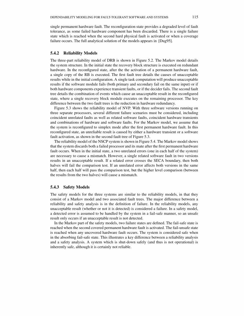
single permanent hardware fault. The reconfiguration state provides a degraded level of faulttolerance, as some failed hardware component has been discarded. There is a single failurestate which is reached when the second hard physical fault is activated or when a coveragefailure occurs. The full analytical solution of the models appears in [Dug95].

5.4.2 Reliability Models

The three-part reliability model of DRB is shown in Figure 5.2. The Markov model detailsthe system structure. In the initial state the recovery block structure is executed on redundanthardware. In the reconfigured state, after the the activation of a permanent hardware fault,a single copy of the RB is executed. The first fault tree details the causes of unacceptableresults while in the initial configuration. A single task computation will produce unacceptableresults if the software module fails (both primary and secondary fail on the same input) or ifboth hardware components experience transient faults, or if the decider fails. The second faulttree details the combination of events which cause an unacceptable result in the reconfiguredstate, where a single recovery block module executes on the remaining processor. The keydifference between the two fault trees is the reduction in hardware redundancy.

Figure 5.3 shows the reliability model of NVP. With three software versions running onthree separate processors, several different failure scenarios must be considered, includingcoincident unrelated faults as well as related software faults, coincident hardware transientsand combinations of hardware and software faults. For the Markov model, we assume thatthe system is reconfigured to simplex mode after the first permanent hardware fault. In thisreconfigured state, an unreliable result is caused by either a hardware transient or a softwarefault activation, as shown in the second fault tree of Figure 5.3.

The reliability model of the NSCP system is shown in Figure 5.4. The Markov model showsthat the system discards both a failed processor and its mate after the first permanent hardwarefault occurs. When in the initial state, a two unrelated errors (one in each half of the system)are necessary to cause a mismatch. However, a single related software fault in two versionsresults in an unacceptable result. If a related error crosses the SECA boundary, then bothhalves will fail the comparison test. If an unrelated error affects both versions in the samehalf, then each half will pass the comparison test, but the higher level comparison (betweenthe results from the two halves) will cause a mismatch.

5.4.3 Safety Models

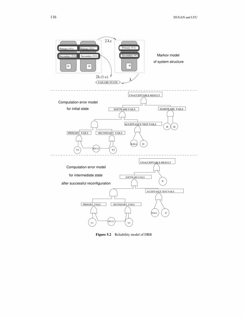
The safety models for the three systems are similar to the reliability models, in that theyconsist of a Markov model and two associated fault trees. The major difference between areliability and safety analysis is in the definition of failure. In the reliability models, anyunacceptable result (whether or not it is detected) is considered a failure. In a safety model,a detected error is assumed to be handled by the system in a fail-safe manner, so an unsaferesult only occurs if an unacceptable result is not detected.

In the Markov part of the safety models, two failure states are defined. The fail-safe state isreached when the second covered permanent hardware fault is activated. The fail-unsafe stateis reached when any uncovered hardware fault occurs. The system is considered safe whenin the absorbing fail-safe state. This illustrates a key difference between a reliability analysisand a safety analysis. A system which is shut-down safely (and thus is not operational) isinherently safe, although it is certainly not reliable.

116 DUGAN and LYU

Markov model

of system structure

Computation error model

for intermediate state

after successful reconfiguration


for initial state

UNACCEPTABLE RESULT

H H

RALL D

H

SECONDARY FAILSPRIMARY FAILS

V2V1RV12

UNACCEPTABLE RESULT

λc2

λ2 (1-c)

H H

Primary (V1)

Secondary (V2)Secondary (V2) Secondary (V2)

H

Primary (V1)

λFAILURE STATE

Primary (V1)

SOFTWARE FAILS

SECONDARY FAILS

V2V1 RV12

ACCEPTANCE TEST FAILS

HARDWARE FAILS

PRIMARY FAILS

ACCEPTANCE TEST FAILS

SOFTWARE FAILS

DRALL

Figure 5.2 Reliability model of DRB


Markov model

of system structure


for initial state



after successful reconfigurationV1 H

UNACCEPTABLE RESULT

λ3 (1-c)

λ c3

UNACCEPTABLE RESULT

H H H H

λ

V1V3V2V1

FAILURE STATE

HH

H

V1 V2V3

2/3

D

VERSION FAILS

RALL

2/3

SOFTWARE FAILS

DECIDER FAILS

HARDWARE FAILS

RV13 RV12RV23

Figure 5.3 Reliability model of NVP

118 DUGAN and LYU

λ4 (1-c)

λ4 c

λ2

V1 V2 V3 V4 V1 V2

H H H H H H

FAILURE STATE

of system structure

Markov model

UNACCEPTABLE RESULT


for initial stateV4 H HV3V1 V2 H H




UNACCEPTABLE RESULT

V1 V2 H H

RV12 RV13 RV23 RV34RV24RV14

DRALL

RV12

DRALL

Figure 5.4 Reliability model of NSCP


Markov model

of system structure


for initial state




(same model for both states)

λc2

Fail Unsafeλ(1-c)

Fail Safe

D

RB UNSAFE

H H

Primary (V1)

Secondary (V2)Secondary (V2) Secondary (V2)

H

Primary (V1)Primary (V1)

λ2 (1-c)

λc

Figure 5.5 Safety model of DRB

The safety model of DRB, shown in Figure 5.5, shows that an acceptance test failure isthe only software cause of an unsafe result. As long as the acceptance test does not accept anincorrect result, then a safe output is assumed to be produced. The hardware redundancy doesnot increase the safety of the system, as the system is vulnerable to the acceptance test in bothstates. An interesting result of a safety analysis is that the hardware redundancy can actuallydecrease the safety of the system, since the system is perfectly safe when in the fail-safe state,and the hardware redundancy delays absorption into this state [Vai93].

The NVP safety model (Figure 5.6) shows that the safety of the NVP system is vulnerableto related faults as well as decider faults. In the Markov model, we assume that the recon-figured state uses two versions (rather than one, as was assumed for the reliability model) soas to increase the opportunity for comparisons between alternatives and thus increase errordetectability.

The NSCP safety model (Figure 5.7) shows the same vulnerability of the NSCP system torelated faults. When the system is fully operational, all 2-way related faults will be detectedby the self-checking arrangements, leaving the system vulnerable only to a decider faults,and a fault affecting all versions similarly. After reconfiguration, a related fault affecting bothremaining versions could also produce an undetected error.

5.5 EXPERIMENTAL DATA ANALYSIS

A quantitative comparison of the three fault tolerant systems described in the previous sec-tion requires an estimation of reasonable values for the model parameters. The estimationof failure probabilities for hardware components has been considered for a number of years,and reasonable estimates exist for generic components (such as a processor). However, the

120 DUGAN and LYU

λ c3


for initial state




Markov model

of system structureH

V1

Fail Unsafe

Fail Safe

λ2 (1-c)

RV13RV23RV12RALL D

RV12

RALL D

H H H

V3V2V1

H

V2

NVP UNSAFE

λ3 (1-c)

c2 λ

NVP UNSAFE

Figure 5.6 Safety model of NVP

estimation of software version failure probability is less accessible, and the estimation of theprobability of related faults is more difficult still. In this section we will describe a methodol-ogy for estimating model parameter values from experimental data followed by a case studyusing a set of experimental data.

Several experiments in multi-version programming have been performed in the past decade.Among other measures, most experiments provide some estimate of the number of times dif-ferent versions fail coincidentally. For example, the NASA-LaRC study involving 20 pro-grams from 4 universities [Eck91] provides a table listing how many instances of coincidentfailures were detected. The Knight-Leveson study of 28 versions [Kni86] provides an es-timated probability of coincident failures. The Lyu-He study [Lyu93] considered three andfive version configurations formed from 12 different versions. These sets of experimental data



for initial state

of system structure

Markov model

λ4 (1-c)

λ4 c

Fail Unsafe Fail Safe

λ2 c

λ2

DRALL




NSCP UNSAFE

RV12

NSCP UNSAFE

V1 V2 V3 V4 V1 V2

H H H H H H

(1-c)

RALL D

Figure 5.7 Safety model of NSCP

can be used to estimated the probabilities for the basic events in a model of a fault tolerantsoftware system.

Coincident failures in different versions can arise from two distinct causes. First, two (ormore) versions may both experience unrelated faults that are activated by the same input. Iftwo programs fail independently, there is always a finite probability that they will fail coin-cidentally, else the programs would not be independent. A coincident failure does not nec-essarily imply that a related fault has been activated. Second, the input may activate a faultthat is related between the two versions. In order to estimate the probabilities of unrelated andrelated faults, we will determine the (theoretical) probability of failure by unrelated faults. Tothe extent that the observed frequency of coincident faults exceeds this value, we will attributethe excess to related faults.

The experimental data is necessarily coarse. As it is infeasible to exhaustively test a sin-gle version, it is more difficult to exhaustively observe every possible instance of coincidentfailures in multiple versions. The experimental data provides an estimate of the probabilitiesof coincident failures, rather than the exact value. Considering the coarseness of the exper-imental data, we will limit ourselves to the estimation of three parameter values: PV , theprobability of an unrelated fault in a version; PRV , the probability of a related fault between

122 DUGAN and LYU

two versions; and PRALL, the probability of a related fault in all versions. To attempt to esti-mate more, for example the probability of a related fault that affects exactly three versions orexactly four versions, seems unreasonable. Notice that we will assume that the versions areall statistically identical, and do not try to attempt to estimate different probabilities of failurefor each individual version, or each individual case of two simultaneous versions.

The first parameter that we estimate is PV , the probability that a single version fails. Theestimate for PV comes from considering F0 (the observed frequency of no failures) and F1

(the observed frequency of exactly one failure). When considering N different versions pro-cessing the same input, the probability that there are no failures is set equal to the observedfrequency of no failures.

F0 = (1− PV )N (1− PRV )(N2 )(1− PRALL) (5.1)

Then, considering the case where only a single failure occurs, we observe that a singlefailure can occur in any of theN programs, and implies that a related fault does not occur (elsemore than one version would be affected). This is then set equal to the observed frequency ofa single failure of the N versions.

F1 = N(1− PV )(N−1)PV (1− PRV )(N2 )(1− PRALL) (5.2)

Dividing equation 5.1 by equation 5.2 yields an estimate for PV .

PV =F1

NF0 + F1(5.3)

Estimating the probability of a related fault between two versions, PRV , is more involved,but follows the same basic procedure. First, consider the case where exactly two versions areobserved to fail coincidentally. This event can be caused by one of three events:

• the simultaneous activation of two unrelated faults, or• the activation of a related fault between two versions or• both (the activation of two unrelated and a related fault between the two versions).

The probabilities of each of these events will be determined separately. The probability thatunrelated faults are simultaneously activated in two versions (and no related faults are acti-vated) is (

N

2

)P 2V (1− PV )(N−2)(1− PRV )(

N2 )(1− PRALL) (5.4)

The probability that a single related fault (and no unrelated fault) is activated is given by

(N

2

)(1− PV )NPRV (1− PRV )((N2 )−1)(1− PRALL) (5.5)

Finally, the probability that both an unrelated fault and two related faults are simultaneouslyactivated is give by

(N

2

)P 2V PRV (1− PV )(N−2)(1− PRV )((N2 )−1)(1− PRALL) (5.6)


V1RV12

RALL

RV13

V2 V3

RV23

ALL VERSIONS FAIL

Figure 5.8 Fault tree model used to estimate PRALL for a 3-version system

Because the three events are disjoint, we can sum their probabilities, and set the sum equal toF2, the observed frequency of two coincident errors.

F2 =

(N

2

)(P 2V + PRV − P 2

V PRV )(1− PV )(N−2)(1− PRV )((N2 )−1)(1− PRALL) (5.7)

Dividing equation 5.7 by 5.2 and performing some algebraic manipulations yields an estimatefor PRV which depends on the experimental data and the previously derived estimate for PV .

PRV =2F2PV (1− PV )− (N − 1)F1P

2V

2F2PV (1− PV ) + (N − 1)F1(1− P 2V )

(5.8)

The estimate for PRALL is more involved, as there are many ways in which all versionscan fail. There may be a related fault between all versions that is activated by the input, orall versions might simultaneously fail from a combination of unrelated and related faults.Consider the case where there are three versions. In addition to the possibility of a singlefault affecting all three versions, all three versions could experience a simultaneous activationof unrelated faults, or one of three combinations of an unrelated and related fault affectingdifferent versions may be activated. The fault tree in Figure 5.8 illustrates the combinationsof events which can cause all three versions to fail coincidentally. A simple (but inelegant)methodology for estimating PRALL could use the previously determined estimates for PVand PRV and repeated guessing for PRALL in the solution of the fault tree in Figure 5.8, untilthe fault tree solution for the probability of simultaneous errors approximates the observedfrequency of all versions failing simultaneously.

The fault tree model for three versions can easily be generalized to the case where thereare N versions. The top event of the fault tree is an OR gate with two inputs, an AND gateshowing all versions failing, and a basic event, representing a related fault that affects allversions simultaneously. The AND gate has N inputs, one for each version. Each of the N

124 DUGAN and LYU

inputs to the AND gate is itself an OR gate with N inputs, all basic events. Each OR gate hasone input representing an unrelated fault in the version, andN − 1 inputs representing relatedfaults with each other possible version.

5.6 A CASE STUDY IN PARAMETER ESTIMATION

In this section we analyze experimental data from a recent multiversion programming exper-iment to determine parameter values for our models of fault-tolerant software systems. Thedata is derived from an experimental implementation of a real-world automatic (i.e., comput-erized) airplane landing system, or so-called “autopilot.” The software systems of this projectwere developed and programmed by 15 programming teams at the University of Iowa and theRockwell/Collins Avionics Division. A total of 40 students (33 from ECE and CS departmentsat the University of Iowa, 7 from the Rockwell International) participated in this project to in-dependently design, code, and test the computerized airplane landing system, as described inthe Lyu-He study [Lyu93].

5.6.1 System Description

The software project in the Lyu-He study was scheduled and conducted in six phases: (1) Ini-tial design phase for four weeks; (2) Detailed design phase for two weeks; (3) Coding phasefor three weeks; (4) Unit testing phase for one week; (5) Integration testing phase for twoweeks; (6) Acceptance testing phase for two weeks. It is noted that the acceptance testing wasa two-step formal testing procedure. In the first step (AT1), each program was run in a testharness of four nominal flight simulation profiles. For the second step (AT2), one extra simu-lation profile, representing an extremely difficult flight situation, was imposed. By the end ofthe acceptance testing phase, 12 of the 15 programs passed the acceptance test successfullyand were engaged in operational testing for further evaluations. The average size of these pro-grams were 1564 lines of uncommented code, or 2558 lines when comments were included.The average fault density of the program versions which passed AT1 was 0.48 faults per thou-sand lines of uncommented code. The fault density for the final versions was 0.05 faults perthousand lines of uncommented code.

5.6.1.1 THE NVP OPERATIONAL ENVIRONMENT

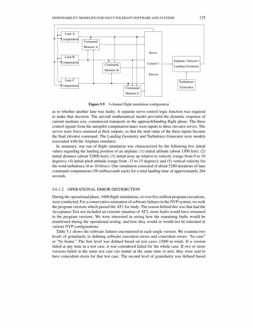
The operational environment for the application was conceived as airplane/autopilot interact-ing in a simulated environment, as shown in Figure 5.9. Three channels of diverse softwareindependently computed a surface command to guide a simulated aircraft along its flight path.To ensure that significant command errors could be detected, random wind turbulences of dif-ferent levels were superimposed in order to represent difficult flight conditions. The individualcommands were recorded and compared for discrepancies that could indicate the presence offaults.

This configuration of a 3-channel flight simulation system consisted of three lanes of con-trol law computation, three command monitors, a servo control, an Airplane model, and aturbulence generator. The lane computations and the command monitors would be the ac-cepted software versions generated by the programming teams. Each lane of independentcomputation monitored the other two lanes. However, no single lane could make the decision


Lane A

Computation

Lane B

Computation

Lane C

Computation

Command

Monitor A

Command

Monitor B

Command

Monitor C

Servo-

Control /

Servos

� � �

� � �

� � �

�

�

Airplane / Sensors /

Landing Geometry

Turbulence

Generator

�

�

Figure 5.9 3-channel flight simulation configuration

as to whether another lane was faulty. A separate servo control logic function was requiredto make that decision. The aircraft mathematical model provided the dynamic response ofcurrent medium size, commercial transports in the approach/landing flight phase. The threecontrol signals from the autopilot computation lanes were inputs to three elevator servos. Theservos were force-summed at their outputs, so that the mid-value of the three inputs becamethe final elevator command. The Landing Geometry and Turbulence Generator were modelsassociated with the Airplane simulator.

In summary, one run of flight simulation was characterized by the following five initialvalues regarding the landing position of an airplane: (1) initial altitude (about 1500 feet); (2)initial distance (about 52800 feet); (3) initial nose up relative to velocity (range from 0 to 10degrees); (4) initial pitch attitude (range from -15 to 15 degrees); and (5) vertical velocity forthe wind turbulence (0 to 10 ft/sec). One simulation consisted of about 5280 iterations of lanecommand computations (50 milliseconds each) for a total landing time of approximately 264seconds.

5.6.1.2 OPERATIONAL ERROR DISTRIBUTION

During the operational phase, 1000 flight simulations, or over five million program executions,were conducted. For a conservative estimation of software failures in the NVP system, we tookthe program versions which passed the AT1 for study. The reason behind this was that had theAcceptance Test not included an extreme situation of AT2, more faults would have remainedin the program versions. We were interested in seeing how the remaining faults would bemanifested during the operational testing, and how they would or would not be tolerated invarious NVP configurations.

Table 5.1 shows the software failures encountered in each single version. We examine twolevels of granularity in defining software execution errors and coincident errors: “by-case”or “by-frame.” The first level was defined based on test cases (1000 in total). If a versionfailed at any time in a test case, it was considered failed for the whole case. If two or moreversions failed in the same test case (no matter at the same time or not), they were said tohave coincident errors for that test case. The second level of granularity was defined based

126 DUGAN and LYU

Table 5.1 Error characteristics for individual versions

Version Id Number of failures Prob. by-case Prob. by-frameβ 510 0.51 0.000096574γ 0 0.0 0.0ε 0 0.0 0.0ζ 0 0.0 0.0η 1 0.001 0.000000189θ 360 0.36 0.000068169κ 0 0.0 0.0λ 730 0.73 0.000138233µ 140 0.14 0.000026510ν 0 0.0 0.0ξ 0 0.0 0.0o 0 0.0 0.0

Average 145.1 0.1451 0.000027472

Table 5.2 Error characteristics for two-version configurations

Category BY-CASE BY-FRAMENumber of cases Frequency Number of cases Frequency

F0 - no errors 53150 0.8053 348522546 0.99994786F1 - single error 11160 0.1691 18128 0.00005201F2 - two coincident 1690 0.0256 46 0.00000013Total 66000 1.0000 348540720 1.000000

on execution time frames (5,280,920 in total). Errors were counted only at the time frameupon which they manifested themselves, and coincident errors were defined to be the multipleprogram versions failing at the same time frame in the same test case (with or without thesame variables and values).

In Table 5.1 we can see that the average failure probability for single version is 0.145measured by-case, or 0.000027 measured by-frame.

5.6.2 Data Analysis and Parameter Estimation

The 12 programs accepted in the Lyu-He experiment were configured in pairs, whose outputswere compared for each test case. Table 5.2 shows the number of times that 0, 1, and 2 errorswere observed in the 2-version configurations. The data from Table 5.2 yields an estimate ofPV = 0.095 for the probability of activation of an unrelated fault in a 2-version configuration,and an estimate of PRV = 0.0167 for the probability of a related fault for the by-case data.The by-frame data in Table 5.2 producesPV = 0.000026 and PRV = 1.3×10−7 as estimates.

Next, the 12 versions were configured in sets of three programs. Table 5.3 shows the numberof times that 0, 1, 2, and 3 errors were observed in the 3-version configurations. The datafrom Table 5.3 yields an estimate of PV = 0.0958 for the probability of activation of anindependent fault in a 3-version configuration. Table 5.4 compares the probability of activationof 1, 2 and 3 faults as predicted by a model assuming independence between versions, with theobserved values. The observed frequency of two simultaneous errors is lower than predicted


Table 5.3 Error characteristics for three-version configurations


F0 - no errors 163370 0.7426 1161707015 0.99991790F1 - single error 51930 0.2360 94835 0.00008163F2 - two coincident 4440 0.0202 550 0.00000047F4 - three coincident 260 0.0012 0 0.0Total 220000 1.0000 1161802400 1.000000

Table 5.4 Comparison of independent model with observed data for 3 versions (by-case)

No. errors activated Independent model Observed frequency0 0.7393 0.74261 0.2350 0.23602 0.0249 0.02023 0.0009 0.0012

by the independent model, while the observed frequency of three simultaneous errors is higherthan predicted. For this set of data we will assume therefore that PRV = 0 and will insteadderive an estimate for PRALL.

Using the assumption that PRV = 0, the probability that three simultaneous errors areactivated is given by

F3 = PV3 + PRALL − PV 3PRALL, (5.9)

yielding an estimate of PRALL = 0.0003 for the by-case data.The by-frame data in Table 5.3 produces PV = 0.000027 as an estimate. For this by-

frame data, when the failure probabilities which are predicted by the independent model arecompared to the actual data (Table 5.5), the observed frequency of two errors is two ordersof magnitude higher than the predicted probability. There were no cases for which all threeprograms produced erroneous results. Thus, we will estimate PRALL = 0 and derive anestimate for PRV = 1.57× 10−7.

The same 12 programs which passed the acceptance testing phase of the software develop-ment process were analyzed in combinations of four programs, the results are shown in Table5.6. The by-case data from Table 5.6 yields an estimate of PV = 0.106 for the probabilityof activation of an unrelated fault in a 4-version configuration. Table 5.7 compares the prob-ability of activation of 1, 2, 3 and 4 faults as predicted by a model assuming independencebetween versions, with the observed values. The observed frequency of two simultaneous er-rors is lower than predicted by the independent model, while the observed frequency of threesimultaneous errors is higher than predicted. For this set of data we will assume that PRV = 0.

Table 5.5 Comparison of independent model with observed data for 3 versions (by-frame)

No. errors activated Independent model Observed frequency0 0.999919 0.9999181 0.000081 0.00008162 2× 10−9 5× 10−7

3 2× 10−14 0.0

128 DUGAN and LYU

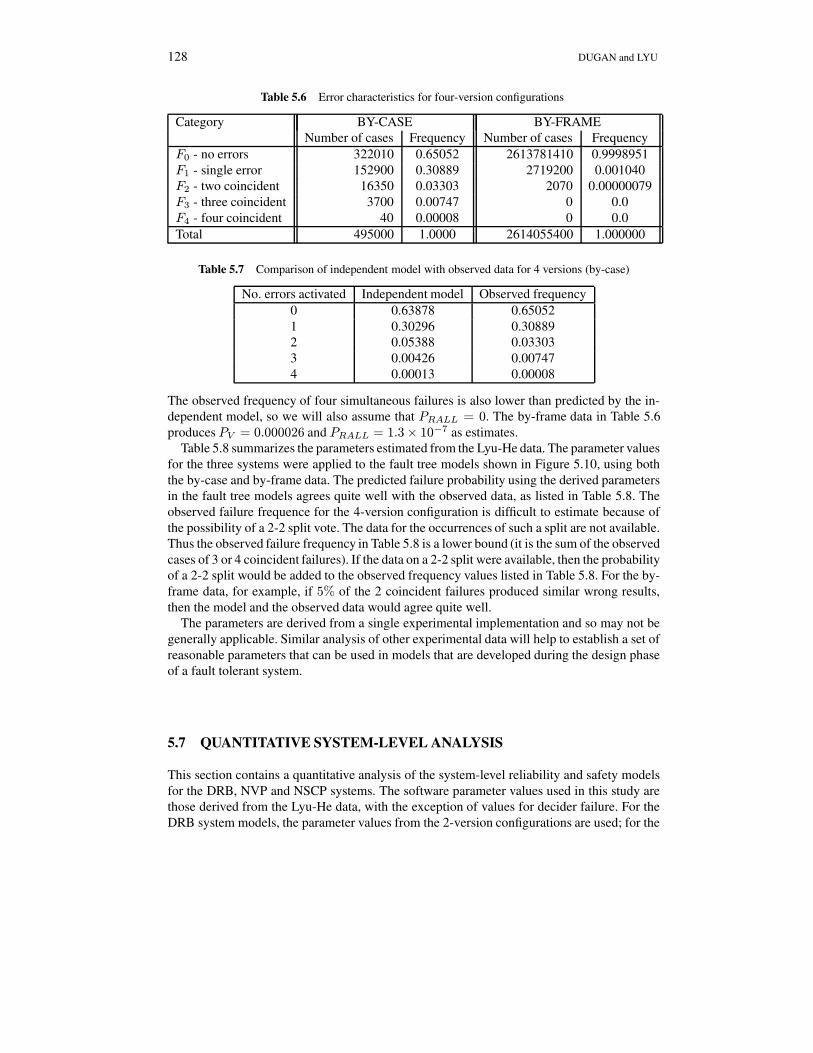
Table 5.6 Error characteristics for four-version configurations


F0 - no errors 322010 0.65052 2613781410 0.9998951F1 - single error 152900 0.30889 2719200 0.001040F2 - two coincident 16350 0.03303 2070 0.00000079F3 - three coincident 3700 0.00747 0 0.0F4 - four coincident 40 0.00008 0 0.0Total 495000 1.0000 2614055400 1.000000

Table 5.7 Comparison of independent model with observed data for 4 versions (by-case)

No. errors activated Independent model Observed frequency0 0.63878 0.650521 0.30296 0.308892 0.05388 0.033033 0.00426 0.007474 0.00013 0.00008

The observed frequency of four simultaneous failures is also lower than predicted by the in-dependent model, so we will also assume that PRALL = 0. The by-frame data in Table 5.6produces PV = 0.000026 and PRALL = 1.3× 10−7 as estimates.

Table 5.8 summarizes the parameters estimated from the Lyu-He data. The parameter valuesfor the three systems were applied to the fault tree models shown in Figure 5.10, using boththe by-case and by-frame data. The predicted failure probability using the derived parametersin the fault tree models agrees quite well with the observed data, as listed in Table 5.8. Theobserved failure frequence for the 4-version configuration is difficult to estimate because ofthe possibility of a 2-2 split vote. The data for the occurrences of such a split are not available.Thus the observed failure frequency in Table 5.8 is a lower bound (it is the sum of the observedcases of 3 or 4 coincident failures). If the data on a 2-2 split were available, then the probabilityof a 2-2 split would be added to the observed frequency values listed in Table 5.8. For the by-frame data, for example, if 5% of the 2 coincident failures produced similar wrong results,then the model and the observed data would agree quite well.

The parameters are derived from a single experimental implementation and so may not begenerally applicable. Similar analysis of other experimental data will help to establish a set ofreasonable parameters that can be used in models that are developed during the design phaseof a fault tolerant system.

5.7 QUANTITATIVE SYSTEM-LEVEL ANALYSIS

This section contains a quantitative analysis of the system-level reliability and safety modelsfor the DRB, NVP and NSCP systems. The software parameter values used in this study arethose derived from the Lyu-He data, with the exception of values for decider failure. For theDRB system models, the parameter values from the 2-version configurations are used; for the


V1 V2 V3

RV12 RV13 RV23

RALL

VERSION FAILS

RELATED FAULT

V2V1

RV12

RV12 RV13 RV14 RV23 RV24 RV34

V2 V3 V4

2-VERSION FAILURE 3-VERSION FAILURE 4-VERSION FAILURE

2/3

V1

3/4

Figure 5.10 Fault tree models for 2, 3 and 4 version systems

Table 5.8 Summary of parameter values derived from Lyu-He data

2-version model 3-version model 4-version modelBY-CASE DATA

PV = 0.095 PV = 0.0958 PV = 0.106PRV = 0.0167 PRV = 0 PRV = 0

PRALL = 0.0003 PRALL = 0Predicted failure probability (from the model)

0.0265 0.0262 0.0044Observed failure probability (from the data)

0.0256 0.0214 0.0076BY-FRAME DATA

PV = 0.000026 PV = 0.000027 PV = 0.000026PRV = 1.3× 10−7 PRV = 1.57× 10−7 PRV = 1.3× 10−7

PRALL = 0 PRALL = 0Predicted failure probability (from the model)

1.31× 10−7 4.73× 10−7 7.8× 10−7

Observed failure probability (from the data)1.32× 10−7 4.73× 10−7 0

130 DUGAN and LYU

NVP system models, we use the parameters derived from the 3-version configurations, whilethe NSCP model uses the parameters derived from the 4-version configurations.

Since no decider failures were observed during the experimental implementation, it is dif-ficult to estimate this probability. The decider used for the recovery block system is an ac-ceptance test, and for this application is likely to be significantly more complex than thecomparator used for the NVP and NSCP systems. For the sake of comparison, for the by-casedata we will assume that the comparator used in the NVP and NSCP systems has a failureprobability of only 0.0001 and that the acceptance test used for the DRB system has a failureprobability of 0.001 . For the by-frame data, the decider is considered to be extremely reliable,with a failure probability of 10−7 for all three systems. If the decider were any less reliable,then its failure probability would dominate the system analysis, and the results would be farless interesting.

Typical permanent failure rates for processors range in the 10−5 per hour range, withtransients perhaps an order of magnitude larger. Thus we will use λp = 10−5 per hour for theMarkov model.

In the by-case scenario, a typical test case contained 5280 time frames, each time framebeing 50 ms., so a typical computation executed for 264 seconds. Assuming that hardwaretransients occur at a rate λt = (10−4/3600) per second, we see that the probability that ahardware transient occurs during a typical test case is

1− e−λt×264 seconds = 7.333× 10−6 (5.10)

We conservatively assume that a hardware transient that occurs anywhere during the executionof a task disrupts the entire computation running on the host.

For the by-frame data, the probability that a transient occurs during a time frame is

1− e−λt×0.05 seconds = 1.4× 10−9 (5.11)

If we further assume that the lifetime of a transient fault is one second, then a transient canaffect as many as 20 time frames. We thus take the probability of a transient to be 20 timesthe value calculated in equation 5.11, or 2.8× 10−8.

Finally, for both the by-case and by-frame scenarios, we assume a fairly typical value forthe coverage parameter in the Markov model, c = 0.999.

5.7.1 Analysis Results

Figure 5.11 compares the predicted reliability of the three systems. Under both the by-caseand by-frame scenarios, the recovery block system is most able to produce a correct result,followed by NVP. NSCP is the least reliable of the three. Of course, these comparisons aredependent on the experimental data used and assumptions made. More experimental data andanalysis are needed to enable a more conclusive comparison.

Figure 5.12 gives a closer look at the comparisons between the NVP and DRB systemsduring the first 200 hours. The by-case data shows a crossover point where NVP is initiallymore reliable but is later less reliable than DRB. Using the by-frame data, there is no crossoverpoint, but the estimates are so small that the differences may not be statistically significant.

Figure 5.13 compares the predicted safety of the three systems. Under the by-case scenario,NSCP is the most likely to produce a safe result, and DRB is an order of magnitude less safethan NVP or NSCP. This difference is caused by the difference in assumed failure probability


0

0.005

0.01

0.015

0.02

0.025

0.03

0.035

0.04

0.045

0.05

0 200 400 600 800 1000

Pro

babi

lity

of U

nacc

epta

ble

Res

ult

time (hours)

DRBNVP

NSCP

0

5e-05

0.0001

0.00015

0.0002

0.00025

0.0003

0.00035

0.0004

0.00045

0 200 400 600 800 1000

Pro

babi

lity

of U

nacc

epta

ble

Res

ult

time (hours)

DRBNVP

NSCP

Figure 5.11 Predicted reliability, by-case data (left) and by-frame data (right)

0.02615

0.0262

0.02625

0.0263

0.02635

0.0264

0.02645

0.0265

0.02655

0.0266

0 50 100 150 200

Pro

babi

lity

of U

nacc

epta

ble

Res

ult

time (hours)

DRBNVP

0

2e-06

4e-06

6e-06

8e-06

1e-05

1.2e-05

1.4e-05

0 50 100 150 200

Pro

babi

lty o

f Una

ccep

tabl

e R

esul

t

time (hours)

DRBNVP

Figure 5.12 Predicted reliability, by-case data (left) and by-frame data (right)

0.0001

0.0002

0.0003

0.0004

0.0005

0.0006

0.0007

0.0008

0.0009

0.001

0.0011

0 200 400 600 800 1000

Pro

babi

lity

of U

nsaf

e R

esul

t

time (hours)

DRBNVP

NSCP

0

5e-06

1e-05

1.5e-05

2e-05

2.5e-05

3e-05

3.5e-05

4e-05

0 200 400 600 800 1000

Pro

babi

lity

of U

nsaf

e R

esul

t

time (hours)

DRBNVP

NSCP

Figure 5.13 Predicted safety, by-case data (left) and by-frame data (right)

132 DUGAN and LYU

Table 5.9 Sensitivity to parameter change for DRB reliability model

BY-CASE Data BY-FRAME DataParameter Result Percent Change Result Percent ChangeNominal 0.0265 2.31× 10−7

PV + 10% 0.0284 7% 2.31× 10−7 no changePRV + 10% 0.0282 6.2% 2.44× 10−7 5.6%PD + 10% 0.0266 1.9% 2.41× 10−7 4.3%

Table 5.10 Sensitivity to parameter change for NVP reliability model


PV + 10% 0.03137 19.9% 5.74× 10−7 0.2%PRV + 10% 6.20× 10−7 8.2%PRALL + 10% 0.0262 0.1%PD + 10% 0.02618 0.04% 5.83× 10−7 1.7%

associated with the decider. Interestingly, the opposite ordering results from the by-framedata. Using the by-frame data to parameterize the models, DRB is predicted to be the safest,while NSCP is the least safe. The reversal of ordering between the by-case and by-frameparameterizations is caused by the relationship between the probabilities of related failure anddecider failure. The by-case data parameter values resulted in related fault probabilities thatwere generally lower than the decider failure probabilities, while the by-frame data resultedin related fault probabilities that were relatively high. In the safety models, since there werefewer events that lead to an unsafe result, this relationship between related faults and deciderfaults becomes significant.

5.8 SENSITIVITY ANALYSIS

5.8.1 Sensitivity of Reliability Model

To see which parameters are the strongest determinant of the system reliability, we increasedeach of the non-zero failure probabilities in turn by 10 percent and observed the effect onthe predicted unreliability. The sensitivity of the predictions to a ten-percent change in inputparameters for the DRB model is shown in Table 5.9. It can be seen that the DRB model ismost sensitive to a change in the probability of an unrelated fault for the by-case data, and toa change in the probability of a related fault for the by-frame data.

Table 5.10 shows, the change in the predicted unreliability (at t = 0) when each of thenon-zero NVP nominal parameters is increased. For the by-case data, a ten percent increasein the probability of an unrelated software fault results in a twenty percent increase in theprobability of an unacceptable result. A ten-percent increase in the probability of a relatedor decider fault activation has an almost negligible effect on the unreliability. For the by-frame data, the proability of a related fault has the largest impact on the probability of anunacceptable result. This is similar to the DRB model.

The sensitivity of the NSCP model to the nominal parameters is shown in Table 5.11. The


Table 5.11 Sensitivity to parameter change for NSCP reliability model


PV + 10% 0.04833 19.6% 8.83× 10−7

PRV + 10% 9.61× 10−7 8.8%PD + 10% 0.04042 0.02% 8.93× 10−7 2.1%

Table 5.12 Sensitivity to parameter change for NVP safety model

BY-CASE Data BY-FRAME DataParameter Result Percent Change Result Percent ChangeNominal 4× 10−4 5.71× 10−7

PRV + 10% 6.18× 10−7 8.2%PRALL + 10% 4.3× 10−4 7.5%PD + 10% 4.1× 10−4 2.5% 5.81× 10−7 1.7%

fault tree models and the sensitivity analysis show that NSCP is vulnerable to related faults,whether they involve versions in the same error confinement area or not.

5.8.2 Sensitivity of Safety Model

The sensitivity analysis for the DRB safety model is simple, as the only software fault con-tributing to an unsafe result is a decider failure. A ten-percent increase in the decider failureprobability leads to a ten percent increase in the probability of an unsafe result.

Table 5.12 shows the sensitivity of the safety prediction to a ten-percent change in the non-zero parameter values. For the by-case data, the prediction is sensitive to a change in eitherthe decider failure probability or the probability of a related fault affecting all versions. Forthe by-frame data, the prediction is much more sensitive to a change in the probability of atwo-way related fault than to a change in the decider failure probability.

Table 5.13 shows the sensitivity of the safety analysis to a change in a parameter value. Achange in the decider failure probability directly affects the system safety prediction for theby-case parameter values.

Table 5.13 Sensitivity to parameter change for NSCP safety model

BY-CASE Data BY-FRAME DataParameter Result Percent Change Result Percent ChangeNominal 1× 10−4 1× 10−7

PRV + 10% 1× 10−7 no changePD + 10% 1.1× 10−4 10% 1.1× 10−7 10%

134 DUGAN and LYU

0.01

0.1

1

0.0001 0.001 0.01 0.1 1

Pro

babi

lty o

f Una

ccep

tabl

e R

esul

t

Probability of Decider Failure

DRBNVP

NSCP

1e-07

1e-06

1e-05

0.0001

0.001

0.01

0.1

1

1e-07 1e-06 1e-05 0.0001 0.001 0.01 0.1 1

Pro

babi

lity

of U

nacc

epta

ble

Res

ult


DRBNVP

NSCP

Figure 5.14 Effect of equal decider failure probabilities on reliability analysis, by-case data (left) andby-frame data (right)

1e-05

0.0001

0.001

0.01

0.1

1

1e-05 0.0001 0.001 0.01 0.1 1

Pro

babi

lty o

f Uns

afe

Res

ult


DRBNVP

NSCP

1e-07

1e-06

1e-05

0.0001

0.001

0.01

0.1

1

1e-07 1e-06 1e-05 0.0001 0.001 0.01 0.1 1

Pro

babi

lty o

f Uns

afe

Res

ult


DRBNVP

NSCP

Figure 5.15 Effect of equal decider failure probabilities on safety analysis, by-case data (left) andby-frame data (right)

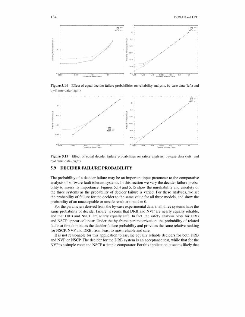
5.9 DECIDER FAILURE PROBABILITY

The probability of a decider failure may be an important input parameter to the comparativeanalysis of software fault tolerant systems. In this section we vary the decider failure proba-bility to assess its importance. Figures 5.14 and 5.15 show the unreliability and unsafety ofthe three systems as the probability of decider failure is varied. For these analyses, we setthe probability of failure for the decider to the same value for all three models, and show theprobability of an unacceptable or unsafe result at time t = 0.

For the parameters derived from the by-case experimental data, if all three systems have thesame probability of decider failure, it seems that DRB and NVP are nearly equally reliable,and that DRB and NSCP are nearly equally safe. In fact, the safety analysis plots for DRBand NSCP appear collinear. Under the by-frame parameterization, the probability of relatedfaults at first dominates the decider failure probability and provides the same relative rankingfor NSCP, NVP and DRB, from least to most reliable and safe.

It is not reasonable for this application to assume equally reliable deciders for both DRBand NVP or NSCP. The decider for the DRB system is an acceptance test, while that for theNVP is a simple voter and NSCP a simple comparator. For this application, it seems likely that


0.01

0.1

1

1e-05 0.0001 0.001 0.01 0.1 1

Pro

babi

lity

of U

nacc

epta

ble

Res

ult

Probability of RB Acceptance Test Failure

DRBNVP

1e-07

1e-06

1e-05

0.0001

0.001

0.01

0.1

1

1e-07 1e-06 1e-05 0.0001 0.001 0.01 0.1 1

Pro

babi

lity

of U

nacc

epta

ble

Res

ult


DRBNVP

Figure 5.16 Effect on reliability of varying acceptance test failure probability for DRB, (while holdingthat of NVP constant), by-case data(left) and by-frame data (right)

1e-05

0.0001

0.001

0.01

0.1

1

1e-05 0.0001 0.001 0.01 0.1 1

Pro

babi

lity

of U

nsaf

e R

esul

t


DRBNSCP

1e-08

1e-07

1e-06

1e-05

0.0001

0.001

0.01

0.1

1

1e-07 1e-06 1e-05 0.0001 0.001 0.01 0.1 1

Pro

babi

lity

of U

nsaf

e R

esul

t


DRBNSCP

Figure 5.17 Effect on safety of varying acceptance test failure probability for DRB, (while holdingthat of NVP constant), by-case data(left) and by-frame data (right)

an acceptance test will be more complicated than a majority voter. The increased complexityis likely to lead to a decrease in reliability, with a corresponding impact on the reliability andsafety of the system. In fact, reliability of DRB will collapse if the acceptance test in DRB isas complex and unreliable as its primary or secondary software versions. For example, if theprobability of failure in acceptance test (PD) is close to PV , which is 0.095 by-case or 0.0004by-frame, then Figure 5.14 indicates that DRB will initially perform the worst comparing withNVP and NSCP.

Figure 5.16 shows how the reliability comparison between DRB and NVP is affected by avariation in the probability of failure for the acceptance test. Figure 5.17 shows how the safetycomparison between DRB and NSCP is affected by a variation in the probability of failure forthe acceptance test. The parameters for the NVP and NSCP analysis were held constant, andthe parameters (other than the probability of acceptance test failure) for the DRB model werealso held constant. Figures 5.16 and 5.17 show that the acceptance test for a recovery blocksystem must be very reliable for it to be comparable in reliability to a similar NVP system, orcomparable in safety to an NSCP system.

136 DUGAN and LYU

5.10 CONCLUSIONS

This chapter proposed a system-level modeling approach to study the reliability and safetybehavior of three types of fault-tolerant architectures: DRB, NVP and NSCP. Using a recentfault-tolerant software project data, we parameterized the models and displayed the probabil-ities of unacceptable results and unsafe results from each of the three architectures.

We used two types of data to parameterize the models. The “by-case” data could detect erroronly at the end of a test case, each representing a complete simulation profile of five thousandprogram iterations, while the “by-frame” data performed error detection and recovery at theend of each iteration. A drastic improvement of safety and reliability were observed in thesecond situation where a finer and more frequent error detection mechanism was assumed bythe decider for each architecture.

In comparing reliability analysis of the three different architectures, DRB performed bet-ter than NVP which in turn was better than NSCP. DRB also enjoyed the feature of relativeinsensitivity to time in its reliability function. This comparison, however, had to be condi-tioned by the probability of decider failures. In the safety analysis NSCP became the best inthe by-case parameters, followed by NVP and then DRB. In the by-frame data the order wasreversed again. As explained in the text, this phenomenon was due to the relative probabilitiesof related faults and decider failure.

We also performed a sensitivity analysis over the three models. It was noted from the by-case data that varying the probability of an unrelated software fault had the major impact tothe system reliability, while from the by-frame data, varying the probability of a related faulthad the largest impact. This could be due to the fact that the by-frame data compares results ina finer granularity level, and was thus more sensitive to related faults among program versions.

In the decider failure analysis, the impact of decider was clearly seen. It was noted thatrelated faults were the dominant cause of failure when the decider failure probability was low,then the decider failure probability dominated as it increased. Moreover, if the acceptancetest in DRB was as unreliable as its application versions, DRB lost its advantage to NVP andNSCP.

Finally, we believe more data points are necessary for at least two purposes. First, themodeling methodology must be validated by considering other experimental data and modelsfor related or correlated faults. Second, the current parameters were derived from a singleexperimental implementation and so may not be generally applicable. Similar analysis ofother experimental data will help to establish a set of reasonable parameters that can be usedin a broader comparison of these and other fault-tolerant architectures.

REFERENCES

[Arl90] Jean Arlat, Karama Kanoun, and Jean-Claude Laprie. Dependability modeling and evaluationof software fault-tolerant systems. IEEE Transactions on Computers, 39(4):504–513, April1990.

[Avi85] Algirdas Avizienis. The N-version approach to fault-tolerant software. IEEE Transactionson Software Engineering, SE-11(12):1491–1501, December 1985.

[Bis86] P.G. Bishop, D.G. Esp, M. Barnes, P. Humphreys, G. Dahl, and J. Lahti. PODS - a project ofdiverse software. IEEE Transactions on Software Engineering, SE-12(9):929–940, Septem-ber 1986.

[Bri93] D. Briere and P. Traverse. Airbus A320/A330/A340 electrical flight controls: a family offault-tolerant systems. In Proc. of the 23rd Symposium on Fault Tolerant Computing, pages


616–623, 1993.[Car84] G.D. Carlow. Architecture of the space shuttle primary avionics software system. Communi-

cations of the ACM, 27(9):926–936, September 1984.[Cia92] Gianfranco Ciardo, Jogesh Muppala, and Kishor Trivedi. Analyzing concurrent and fault-

tolerant software using stochastic reward nets. Journal of Parallel and Distributed Comput-ing, 15:255–269, 1992.

[Dug94] Joanne Bechta Dugan. Experimental analysis of models for correlation in multiversion soft-ware. In Proc. of the International Symposium on Software Reliability Engineering, 1994.

[Dug95] Joanne Bechta Dugan. Software reliability analysis using fault trees. In Michael R. Lyu,editor, McGraw-Hill Software Reliability Engineering Handbook. McGraw-Hill, New York,NY, 1995.

[Dug89] Joanne Bechta Dugan and K. S. Trivedi. Coverage modeling for dependability analysis offault-tolerant systems. IEEE Transactions on Computers, 38(6):775–787, 1989.

[Eck91] Dave E. Eckhardt, Alper K. Caglayan, John C. Knight, Larry D. Lee, David F. McAllister,Mladen A. Vouk, and John P.J. Kelly. An experimental evaluation of software redundancy asa strategy for improving reliability. IEEE Transactions on Software Engineering, 17(7), July1991.

[Eck85] Dave E. Eckhardt and Larry D. Lee. Theoretical basis for the analysis of multiversion soft-ware subject to coincident errors. IEEE Transactions on Software Engineering, 11(12):1511–1517, December 1985.

[Gei90] Robert Geist and Kishor Trivedi. Reliability estimation of fault-tolerant systems: tools andtechniques. IEEE Computer, pages 52–61, July 1990.

[Grn80] A. Grnarov, J. Arlat, and A. Avizienis. On the performance of software fault tolerance strate-gies. In Digest of 10th FTCS, pages 251–253, Kyoto, Japan, October 1980.

[Gun88] Gunnar Hagelin. ERICSSON safety system for railway control. In U. Voges, editor, SoftwareDiversity in Computerized Control Systems, pages 11–21. Springer-Verlag, 1988.

[Hec86] Herbert Hecht and Myron Hecht. Fault-tolerant software. In D.K.Pradhan, editor, Fault-Tolerant Computing: Theory and Techniques, 2:658–696. Prentice-Hall, 1986.

[Hil85] A. D. Hills. Digital fly-by-wire experience. In Proc. AGARD Lecture Series, (143), October1985.

[Joh88] Allen M. Johnson and Miroslaw Malek. Survey of software tools for evaluating reliabilityavailability, and serviceability. ACM Computing Surveys, 20(4):227–269, December 1988.

[Kim89] K.H. Kim and Howard O. Welch. Distributed execution of recovery blocks: an approach foruniform treatment of hardware and software faults in real-time applications. IEEE Transac-tions on Computers, 38(5):626–636, May 1989.

[Kni86] John C. Knight and Nancy G. Leveson. An experimental evaluation of the assumption ofindependence in multiversion programming. IEEE Transactions on Software Engineering,SE-12(1):96–109, January 1986.

[Lal88] Jaynarayan H. Lala and Linda S. Alger. Hardware and software fault tolerance: a unified ar-chitectural approach. In Proc. IEEE International Symposium on Fault-Tolerant Computing,FTCS-18, pages 240–245, June 1988.

[Lap84] Jean-Claude Laprie. Dependability evaluation of software systems in operation. IEEE Trans-actions on Software Engineering, SE-10(6):701–714, November 1984.

[Lap90] Jean-Claude Laprie, Jean Arlat, Christian Beounes, and Karama Kanoun. Definition andAnalysis of Hardware- and Software- Fault-Tolerant Architectures. IEEE Computer, pages39–51, July 1990.

[Lap92] Jean-Claude Laprie and Karama Kanoun. X-ware reliability and availability modeling. IEEETransactions on Software Engineering, pages 130–147, February, 1992.

[Lit89] Bev Littlewood and Douglas R. Miller. Theoretical basis for the analysis of multiversion soft-ware subject to coincident errors. IEEE Transactions on Software Engineering, 15(12):1596–1614, December 1989.

[Lyu93] Michael R. Lyu and Yu-Tao He. Improving the N-version programming process through theevolution of a design paradigm. IEEE Transactions on Reliability, 42(2):179–189, June 1993.

[Nic90] Victor F. Nicola and Ambuj Goyal. Modeling of correlated failures and community errorrecovery in multiversion software. IEEE Transactions on Software Engineering, 16(3), March1990.

138 DUGAN and LYU

[Ram81] C. V. Ramamoorthy, Y. Mok, F. Bastani, G. Chin, , and K. Suzuki. Application of a method-ology for the development and validation of reliable process control software. IEEE Trans-actions on Software Engineering, SE-7(6):537–555, November 1981.

[Ran75] Brian Randell. System structure for software fault tolerance. IEEE Transactions on SoftwareEngineering, SE-1(2):220–232, June 1975.

[Sco87] R. Keith Scott, James W. Gault, and David F. McAllister. Fault-tolerant software reliabilitymodeling. IEEE Transactions on Software Engineering, SE-13(5):582–592, May 1987.

[Shi84] Kang G. Shin and Yann-Hang Lee. Evaluation of error recovery blocks used for cooperatingprocesses. IEEE Transactions on Software Engineering, SE-10(6):692–700, November 1984.

[Sta87] George. E. Stark. Dependability evaluation of integrated hardware/software systems. IEEETransactions on Reliability, pages 440–444, October 1987.

[Tai93] Ann T. Tai, John F. Meyer, and Algirdas Avizienis. Performability enhancement of fault-tolerant software. IEEE Transactions on Reliability, pages 227–237, June 1993.

[Tra88] Pascal Traverse. Airbus and ATR system architecture and specification. In U. Voges, editor,Software Diversity in Computerized Control Systems, pages 95–104. Springer-Verlag, June1988.

[Vai93] Nitin H. Vaidya and Dhiraj K. Pradhan. Fault-tolerant design strategies for high reliabilityand safety. IEEE Transactions on Computers, 42(10), October 1993.

[Vog88] Udo Voges. Use of diversity in experimental reactor safety systems. In U. Voges, editor,Software Diversity in Computerized Control Systems, pages 29–49. Springer-Verlag, 1988.

[Wei91] Liubao Wei. A Model Based Study of Workload Influence on Computing System Dependabil-ity. PhD thesis, University of Michigan, 1991.

[You84] L. J. Yount. Architectural solutions to safety problems of digital flight-critical systems forcommercial transports. In Proc. AIAA/IEEE Digital Avionics Systems Conference, pages 1–8,December 1984.

Documents

Contentslyu/book/sft/pdf/chap5.pdf · Contents 5 Dependability ... 5.2 SYSTEM DESCRIPTIONS ... architectures (DRB, NVP, and NSCP) being considered in this chapter. The systems are