L. Vandenberghe ECE133A (Fall 2021)

7. Linear equations

• QR factorization method

• factor and solve

• LU factorization

7.1

QR factorization and matrix inverse

QR factorization of nonsingular matrix

every nonsingular 𝐴 ∈ R𝑛×𝑛 has a QR factorization

𝐴 = 𝑄𝑅

• 𝑄 ∈ R𝑛×𝑛 is orthogonal (𝑄𝑇𝑄 = 𝑄𝑄𝑇 = 𝐼)

• 𝑅 ∈ R𝑛×𝑛 is upper triangular with positive diagonal elements

Inverse from QR factorization: the inverse 𝐴−1 can be written as

𝐴−1 = (𝑄𝑅)−1 = 𝑅−1𝑄−1 = 𝑅−1𝑄𝑇

Linear equations 7.2

Solving linear equations by QR factorization

Algorithm: to solve 𝐴𝑥 = 𝑏 with nonsingular 𝐴 ∈ R𝑛×𝑛,

1. factor 𝐴 as 𝐴 = 𝑄𝑅

2. compute 𝑦 = 𝑄𝑇𝑏

3. solve 𝑅𝑥 = 𝑦 by back substitution

Complexity: 2𝑛3 + 3𝑛2 ≈ 2𝑛3 flops

• QR factorization: 2𝑛3

• matrix-vector multiplication: 2𝑛2

• back substitution: 𝑛2

Linear equations 7.3

Multiple right-hand sides

consider 𝑘 sets of linear equations with the same coefficient matrix 𝐴:

𝐴𝑥1 = 𝑏1, 𝐴𝑥2 = 𝑏2, . . . , 𝐴𝑥𝑘 = 𝑏𝑘

• equivalently, solve 𝐴𝑋 = 𝐵 where 𝐵 is 𝑛 × 𝑘 matrix with columns 𝑏1, . . . , 𝑏𝑘

• can be solved in 2𝑛3 + 3𝑘𝑛2 flops if we reuse the factorization 𝐴 = 𝑄𝑅

• for 𝑘 � 𝑛, cost is roughly equal to cost of solving one equation (2𝑛3)

Application: to compute 𝐴−1, solve the matrix equation 𝐴𝑋 = 𝐼

• equivalent to 𝑛 equations

𝑅𝑥1 = 𝑄𝑇𝑒1, 𝑅𝑥2 = 𝑄𝑇𝑒2, . . . , 𝑅𝑥𝑛 = 𝑄𝑇𝑒𝑛

(𝑥𝑖 is column 𝑖 of 𝑋 and 𝑄𝑇𝑒𝑖 is transpose of 𝑖th row of 𝑄)

• complexity is 2𝑛3 + 𝑛3 = 3𝑛3 (here the 2nd term 𝑛3 is not negligible)

Linear equations 7.4

Outline

• QR factorization method

• factor and solve

• LU factorization

Factor–solve approach

to solve 𝐴𝑥 = 𝑏, first write 𝐴 as a product of “simple” matrices

𝐴 = 𝐴1𝐴2 · · · 𝐴𝑘

then solve (𝐴1𝐴2 · · · 𝐴𝑘)𝑥 = 𝑏 by solving 𝑘 equations

𝐴1𝑧1 = 𝑏, 𝐴2𝑧2 = 𝑧1, . . . , 𝐴𝑘−1𝑧𝑘−1 = 𝑧𝑘−2, 𝐴𝑘𝑥 = 𝑧𝑘−1

Examples

• QR factorization: 𝑘 = 2, 𝐴 = 𝑄𝑅

• LU factorization (this lecture)

• Cholesky factorization (later)

Linear equations 7.5

Complexity of factor–solve method

#flops = 𝑓 + 𝑠

• 𝑓 is complexity of factoring 𝐴 as 𝐴 = 𝐴1𝐴2 · · · 𝐴𝑘 (factorization step)

• 𝑠 is complexity of solving the 𝑘 equations for 𝑧1, 𝑧2, . . . 𝑧𝑘−1, 𝑥 (solve step)

• usually 𝑓 � 𝑠

Example: solving linear equations using the QR factorization

𝑓 = 2𝑛3, 𝑠 = 3𝑛2

Linear equations 7.6

Outline

• QR factorization method

• factor and solve

• LU factorization

LU factorization

LU factorization without pivoting

𝐴 = 𝐿𝑈

• 𝐿 unit lower triangular, 𝑈 upper triangular

• does not always exist (even if 𝐴 is nonsingular)

LU factorization (with row pivoting)

𝐴 = 𝑃𝐿𝑈

• 𝑃 permutation matrix, 𝐿 unit lower triangular, 𝑈 upper triangular

• exists if and only if 𝐴 is nonsingular (see later)

Complexity: (2/3)𝑛3 if 𝐴 is 𝑛 × 𝑛

Linear equations 7.7

Solving linear equations by LU factorization

Algorithm: to solve 𝐴𝑥 = 𝑏 with nonsingular 𝐴 of size 𝑛 × 𝑛

1. factor 𝐴 as 𝐴 = 𝑃𝐿𝑈 ((2/3)𝑛3 flops)

2. solve (𝑃𝐿𝑈)𝑥 = 𝑏 in three steps

(a) permutation: 𝑧1 = 𝑃𝑇𝑏 (0 flops)(b) forward substitution: solve 𝐿𝑧2 = 𝑧1 (𝑛2 flops)(c) back substitution: solve 𝑈𝑥 = 𝑧2 (𝑛2 flops)

Complexity: (2/3)𝑛3 + 2𝑛2 ≈ (2/3)𝑛3 flops

this is the standard method for solving 𝐴𝑥 = 𝑏

Linear equations 7.8

Multiple right-hand sides

two equations with the same matrix 𝐴 (nonsingular and 𝑛 × 𝑛):

𝐴𝑥 = 𝑏, 𝐴𝑥 = �̃�

• factor 𝐴 once

• forward/back substitution to get 𝑥

• forward/back substitution to get 𝑥

complexity: (2/3)𝑛3 + 4𝑛2 ≈ (2/3)𝑛3

Exercise: propose an efficient method for solving

𝐴𝑥 = 𝑏, 𝐴𝑇𝑥 = �̃�

Linear equations 7.9

LU factorization and matrix inverse

suppose 𝐴 is nonsingular and 𝑛 × 𝑛, with LU factorization

𝐴 = 𝑃𝐿𝑈

• inverse from LU factorization

𝐴−1 = (𝑃𝐿𝑈)−1 = 𝑈−1𝐿−1𝑃𝑇

• gives interpretation of solve step: we evaluate

𝑥 = 𝐴−1𝑏 = 𝑈−1𝐿−1𝑃𝑇𝑏

in three steps𝑧1 = 𝑃𝑇𝑏, 𝑧2 = 𝐿−1𝑧1, 𝑥 = 𝑈−1𝑧2

Linear equations 7.10

Computing the inverse

solve 𝐴𝑋 = 𝐼 column by column

• one LU factorization of 𝐴: 2𝑛3/3 flops

• 𝑛 solve steps: 2𝑛3 flops

• total: (8/3)𝑛3 flops

slightly faster methods exist that exploit structure in right-hand side 𝐼

Conclusion: do not solve 𝐴𝑥 = 𝑏 by multiplying 𝐴−1 with 𝑏

Linear equations 7.11

LU factorization without pivoting

[𝐴11 𝐴1,2:𝑛𝐴2:𝑛,1 𝐴2:𝑛,2:𝑛

]=

[1 0

𝐿2:𝑛,1 𝐿2:𝑛,2:𝑛

] [𝑈11 𝑈1,2:𝑛0 𝑈2:𝑛,2:𝑛

]=

[𝑈11 𝑈1,2:𝑛

𝑈11𝐿2:𝑛,1 𝐿2:𝑛,1𝑈1,2:𝑛 + 𝐿2:𝑛,2:𝑛𝑈2:𝑛,2:𝑛

]Recursive algorithm

• determine first row of 𝑈 and first column of 𝐿

𝑈11 = 𝐴11, 𝑈1,2:𝑛 = 𝐴1,2:𝑛, 𝐿2:𝑛,1 =1𝐴11

𝐴2:𝑛,1

• factor the (𝑛 − 1) × (𝑛 − 1)-matrix 𝐴2:𝑛,2:𝑛 − 𝐿2:𝑛,1𝑈1,2:𝑛 as

𝐴2:𝑛,2:𝑛 − 𝐿2:𝑛,1𝑈1,2:𝑛 = 𝐿2:𝑛,2:𝑛𝑈2:𝑛,2:𝑛

this is an LU factorization (without pivoting) of size (𝑛 − 1) × (𝑛 − 1)

Linear equations 7.12

Example

LU factorization (without pivoting) of

𝐴 =

8 2 94 9 46 7 9

write as 𝐴 = 𝐿𝑈 with 𝐿 unit lower triangular, 𝑈 upper triangular

𝐴 =

8 2 94 9 46 7 9

=

1 0 0𝐿21 1 0𝐿31 𝐿32 1

𝑈11 𝑈12 𝑈130 𝑈22 𝑈230 0 𝑈33

Linear equations 7.13

Example

• first row of 𝑈, first column of 𝐿:8 2 94 9 46 7 9

=

1 0 01/2 1 03/4 𝐿32 1

8 2 90 𝑈22 𝑈230 0 𝑈33

• second row of 𝑈, second column of 𝐿:[

9 47 9

]−[

1/23/4

] [2 9

]=

[1 0𝐿32 1

] [𝑈22 𝑈230 𝑈33

][

8 −1/211/2 9/4

]=

[1 0

11/16 1

] [8 −1/20 𝑈33

]• third row of 𝑈: 𝑈33 = 9/4 + 11/32 = 83/32

Conclusion

𝐴 =

8 2 94 9 46 7 9

=

1 0 01/2 1 03/4 11/16 1

8 2 90 8 −1/20 0 83/32

Linear equations 7.14

Not every nonsingular 𝐴 can be factored as 𝐴 = 𝐿𝑈

𝐴 =

1 0 00 0 20 1 −1

=

1 0 0𝐿21 1 0𝐿31 𝐿32 1

𝑈11 𝑈12 𝑈130 𝑈22 𝑈230 0 𝑈33

• first row of 𝑈, first column of 𝐿:

1 0 00 0 20 1 −1

=

1 0 00 1 00 𝐿32 1

1 0 00 𝑈22 𝑈230 0 𝑈33

• second row of 𝑈, second column of 𝐿:[

0 21 −1

]=

[1 0𝐿32 1

] [𝑈22 𝑈230 𝑈33

]𝑈22 = 0, 𝑈23 = 2, 𝐿32 · 0 = 1 ?

Linear equations 7.15

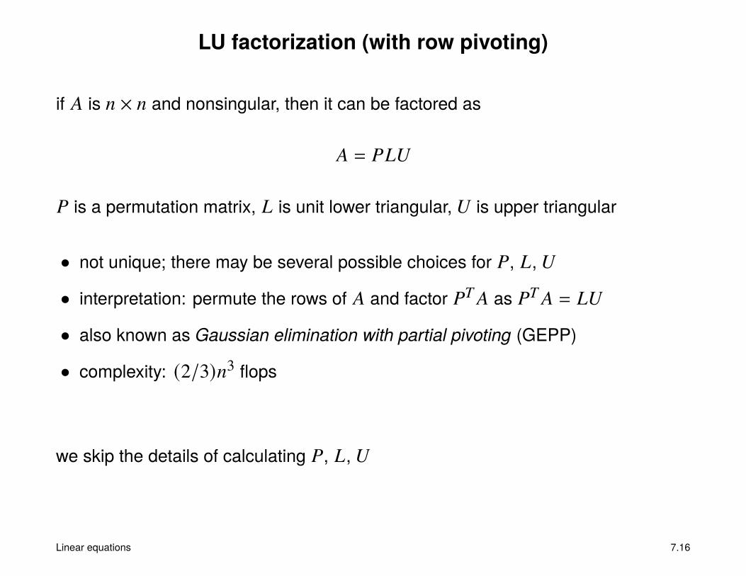
LU factorization (with row pivoting)

if 𝐴 is 𝑛 × 𝑛 and nonsingular, then it can be factored as

𝐴 = 𝑃𝐿𝑈

𝑃 is a permutation matrix, 𝐿 is unit lower triangular, 𝑈 is upper triangular

• not unique; there may be several possible choices for 𝑃, 𝐿, 𝑈

• interpretation: permute the rows of 𝐴 and factor 𝑃𝑇𝐴 as 𝑃𝑇𝐴 = 𝐿𝑈

• also known as Gaussian elimination with partial pivoting (GEPP)

• complexity: (2/3)𝑛3 flops

we skip the details of calculating 𝑃, 𝐿, 𝑈

Linear equations 7.16

Example

0 5 52 9 06 8 8

=

0 0 10 1 01 0 0

1 0 01/3 1 00 15/19 1

6 8 80 19/3 −8/30 0 135/19

the factorization is not unique; the same matrix can be factored as

0 5 52 9 06 8 8

=

0 1 01 0 00 0 1

1 0 00 1 03 −19/5 1

2 9 00 5 50 0 27

Linear equations 7.17

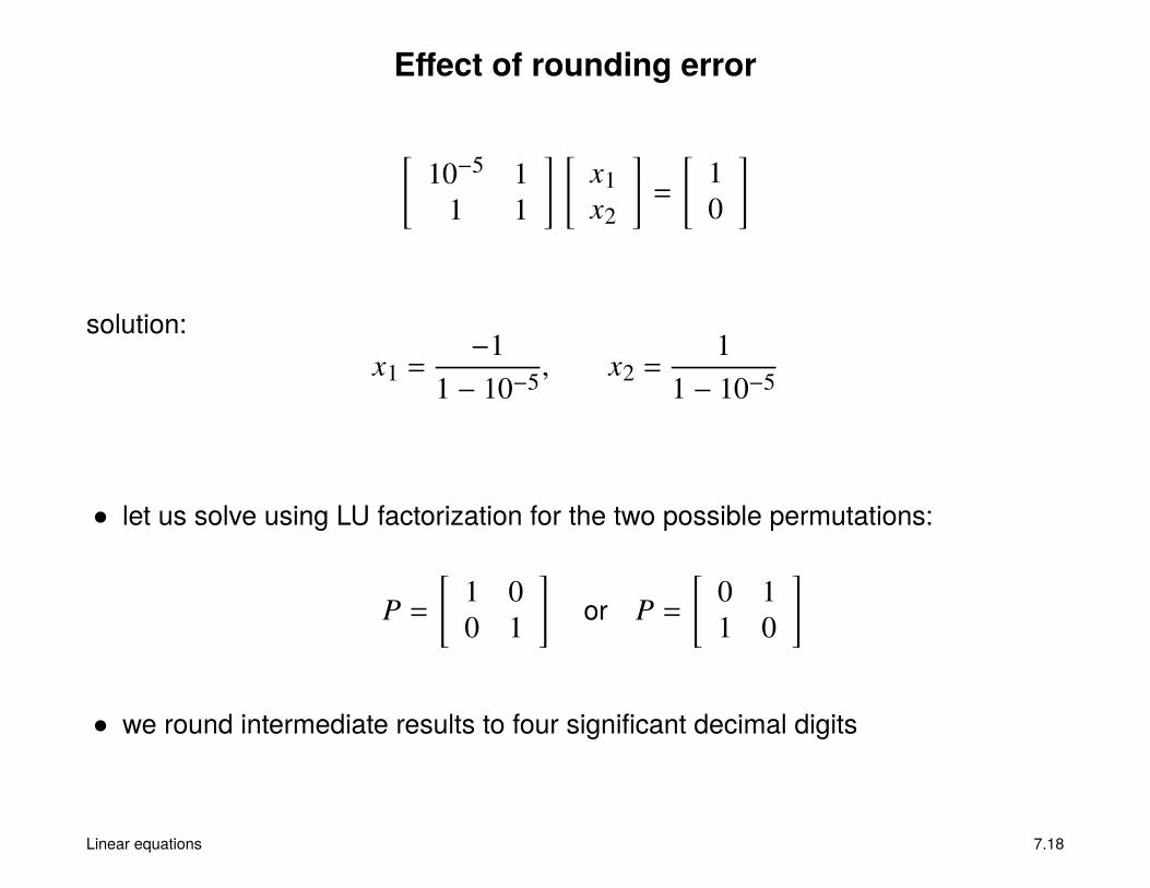
Effect of rounding error

[10−5 1

1 1

] [𝑥1𝑥2

]=

[10

]

solution:𝑥1 =

−11 − 10−5 , 𝑥2 =

11 − 10−5

• let us solve using LU factorization for the two possible permutations:

𝑃 =

[1 00 1

]or 𝑃 =

[0 11 0

]• we round intermediate results to four significant decimal digits

Linear equations 7.18

First choice: 𝑃 = 𝐼 (no pivoting)[10−5 1

1 1

]=

[1 0

105 1

] [10−5 1

0 1 − 105

]• 𝐿, 𝑈 rounded to 4 significant decimal digits

𝐿 =

[1 0

105 1

], 𝑈 =

[10−5 1

0 −105

]• forward substitution[

1 0105 1

] [𝑧1𝑧2

]=

[10

]=⇒ 𝑧1 = 1, 𝑧2 = −105

• back substitution[10−5 1

0 −105

] [𝑥1𝑥2

]=

[1

−105

]=⇒ 𝑥1 = 0, 𝑥2 = 1

error in 𝑥1 is 100%Linear equations 7.19

Second choice: interchange rows[1 1

10−5 1

]=

[1 0

10−5 1

] [1 10 1 − 10−5

]• 𝐿, 𝑈 rounded to 4 significant decimal digits

𝐿 =

[1 0

10−5 1

], 𝑈 =

[1 10 1

]• forward substitution[

1 010−5 1

] [𝑧1𝑧2

]=

[01

]=⇒ 𝑧1 = 0, 𝑧2 = 1

• backward substitution[1 10 1

] [𝑥1𝑥2

]=

[01

]=⇒ 𝑥1 = −1, 𝑥2 = 1

error in 𝑥1, 𝑥2 is about 10−5

Linear equations 7.20

Conclusion: rounding error and LU factorization

• for some choices of 𝑃, small errors in the algorithm can cause very large errorsin the solution

• this is called numerical instability: for the first choice of 𝑃 in the example, thealgorithm is unstable; for the second choice of 𝑃, it is stable

• from numerical analysis: there is a simple rule for selecting a good permutation

(we skip the details, since we skipped the details of the factorization)

Linear equations 7.21

Sparse linear equations

if 𝐴 is sparse, it is usually factored as

𝐴 = 𝑃1𝐿𝑈𝑃2

𝑃1 and 𝑃2 are permutation matrices

• interpretation: permute rows and columns of 𝐴 and factor �̃� = 𝑃𝑇1 𝐴𝑃𝑇2

�̃� = 𝐿𝑈

• choice of 𝑃1 and 𝑃2 greatly affects the sparsity of 𝐿 and 𝑈: several heuristicmethods exist for selecting good permutations

• in practice: #flops � (2/3)𝑛3; exact value depends on 𝑛, number of nonzeroelements, sparsity pattern

Linear equations 7.22

Conclusion

different levels of detail in understanding how linear equation solvers work

Highest level

• x = A \ b costs (2/3)𝑛3

• more efficient than x = inv(A) * b

Intermediate level: factorization step 𝐴 = 𝑃𝐿𝑈 followed by solve step

Lowest level: details of factorization 𝐴 = 𝑃𝐿𝑈

• for most applications, level 1 is sufficient

• in some situations (e.g., multiple right-hand sides) level 2 is useful

• level 3 is important for experts who write numerical libraries

Linear equations 7.23