Embed Size (px)
Citation preview

LungNet: Shallow CNN models for NSCLC
P R I TAM M U KH ER J EE
In collaboration with
Mu Zhou, Edward Lee, Sandy Napel, Simon Wong,
Ann Leung and Olivier Gevaert, Stanford University,
Anne Schicht and Alexander Thieme, Charité Universitätsmedizin, Berlin
Yoganand Balagurunathan and Robert Gillies, Moffitt Cancer Center
Motivation
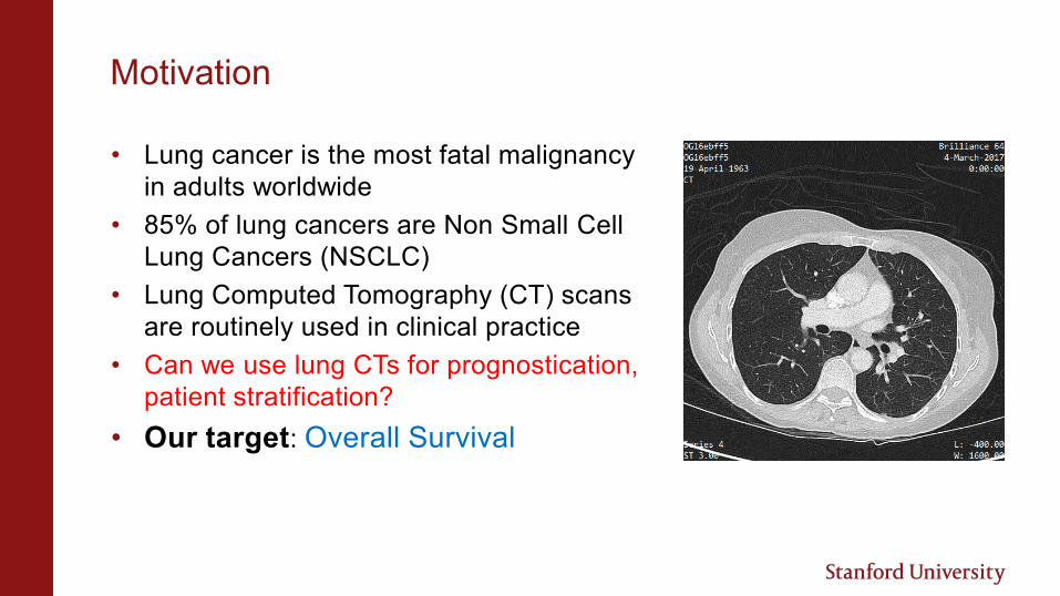
• Lung cancer is the most fatal malignancy
in adults worldwide
• 85% of lung cancers are Non Small Cell
Lung Cancers (NSCLC)
• Lung Computed Tomography (CT) scans
are routinely used in clinical practice
• Can we use lung CTs for prognostication,
patient stratification?
• Our target: Overall Survival

Data: Multi-institutional Cohort
We collected lung CT image data from four institutions:
• Cohort 1 from Stanford Hospital (n=129)
• Now publicly available on TCIA:
http://doi.org/10.7937/K9/TCIA.2017.7hs46erv
• Cohort 2 from Moffitt Cancer Center (n=185)
• Soon to be made available
• Cohort 3 from MAASTRO Clinic, The Netherlands (n=311)
• Publicly available on TCIA:
http://doi.org/10.7937/K9/TCIA.2015.PF0M9REI
• Cohort 4 from Charité – Universitätsmedizin, Berlin (n=84)

Data: Patient characteristics
Characteristic Institutional Cohorts
Cohort 1 Cohort 2 Cohort 3 Cohort 4
Number of patients 129 185 311 84
Age (yrs, Mean ± SD) 69.40 ± 8.47 67.65 ± 10.13 67.05 ± 9.07
Sex (n Male, %) 101 (78.3%) 82 (44.3%) 220 (70.7%) 64 (76.2%)
Smoking history 20 (15.5%) 38 (20.5%)
Histology
Adenocarcinoma 100 (77.5%) 107 (57.8%) 32 (10.3%) 36 (42.9%)
Squamous Carcinoma 29 (22.5%) 50 (27%) 84 (27%) 44 (52.4%)
Other histology
type(s)28 (15.2%) 195 (62.7%) 4 (4.8%)
Survival time (dys,
Mean)889 1021 609 944
Survival time (dys,
Std)671 504 457 710
Staging status
Stage 1 67 97 81 5
Stage 2 42 32 26 10
Stage 3 15 38 73 69
Stage 4 5 18 131 0
Methodology
• Convolutional Neural Networks
• Nodules segmented by radiologists
• Input: 3D patch containing the nodule and corresponding masks and clinical variables (optional)
• Output: Hazard ratio that can be used to stratify patients
• Data augmentation:
• Random flips
• Random crops
• Random brightness change
• Addition of a small amount of noise
• Small rotations

Model Architecture: Imaging Only
Conv
3d
Conv
3d
M
a
xp
o
o
l
M
a
xp
o
o
l
Conv
3d
Conv
3d
Conv
3d
Conv
3d
F
C
1
F
C
1
F
C
2
F
C
2
F
C
3
F
C
3
Hazard Ratiotrained with
Cox Regression Loss
16x3x3 16x3x316x3x3
1286464
K=2, s=2

Con
v 3d
Con
v 3d
M
a
xp
o
o
l
M
a
xp
o
o
l
Con
v 3d
Con
v 3d
Con
v 3d
Con
v 3d
F
C
1
F
C
1
F
C
2
F
C
2
F
C
3
F
C
3
Hazard Ratiotrained with
Cox Regression Loss
Model Architecture: With Clinical features
Clinical
features (one hot
encoded):
Age, sex,
histology,
stage
C
o
n
c
a
t
C
o
n
c
a
t

Training and Validation
• 80-20 train-validation split while training
• Monitor the validation loss while training and save best models
• Training for 100 epochs with a cyclic learning rate, batch size=64
• Round-robin training and testing with cohorts 1, 2 and 3
• Train on two cohorts and test on the third
• Cohort 4 is used for external validation
• Model trained on cohorts 1, 2 and 3
• Tested on cohort 4
• Cox Proportional hazards models with clinical features (sex, age, histology, stage) for benchmarking with same training/validation method

Results: Stratification of patients into risk groups
Cohort 1
LungNet Clinical model

Results: Stratification of patients into risk groups
Cohort 2
LungNet Clinical model

Results: Stratification of patients into risk groups
Cohort 3
LungNet Clinical model

Results: Stratification of patients into risk groups
Cohort 4
LungNet Clinical model
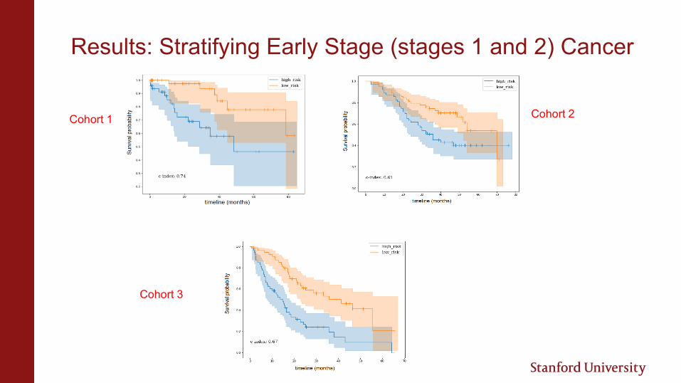
Results: Stratifying Early Stage (stages 1 and 2) Cancer
Cohort 1
Cohort 3
Cohort 2

Results: Takeaways and Caveats
• Adding clinical data did not improve model performance
• Performed reasonably well on early stage cancers as well
• Separate models for adenocarcinoma and SCC?
• Not enough data unfortunately
• Inter-reader variability of segmentations not analyzed
• Random crops for robustness
• Variability in CT acquisition parameters not explicitly analyzed
• Random brightness shifts and small added noise
• Ultimately seems to generalize quite well across institutions!

Additional Slide 1: Cox Regression Loss
• 𝜃: parameters to train
• ℎ𝜃: prediction of the model
• E: event of interest
• 𝑇𝑖: time at which the event occurs for sample i
• 𝑅(𝑇𝑖) : set of samples which have not seen E until 𝑇𝑖
𝑙 𝜃 = −1
𝑁𝐸=1
𝑖:𝐸𝑖=1
ℎ𝜃(𝑥𝑖) − log
𝑗∈𝑅(𝑇𝑖)
𝑒ℎ𝜃 (𝑥𝑗)

Additional Slide 2: Learning rate modifier
Rationale: escape saddle points by increasing learning rate in a
cyclic fashion – may allow faster convergence