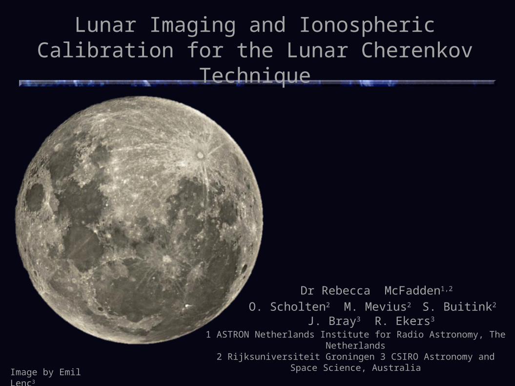
Lunar Imaging and Ionospheric Calibration for the Lunar Cherenkov Technique

O. Scholten2 M. Mevius2 S. Buitink2 J. Bray3 R. Ekers3

1 ASTRON Netherlands Institute for Radio Astronomy, The Netherlands2 Rijksuniversiteit Groningen 3 CSIRO Astronomy and Space Science, Australia

Dr Rebecca McFadden1,2

Image by Emil Lenc3

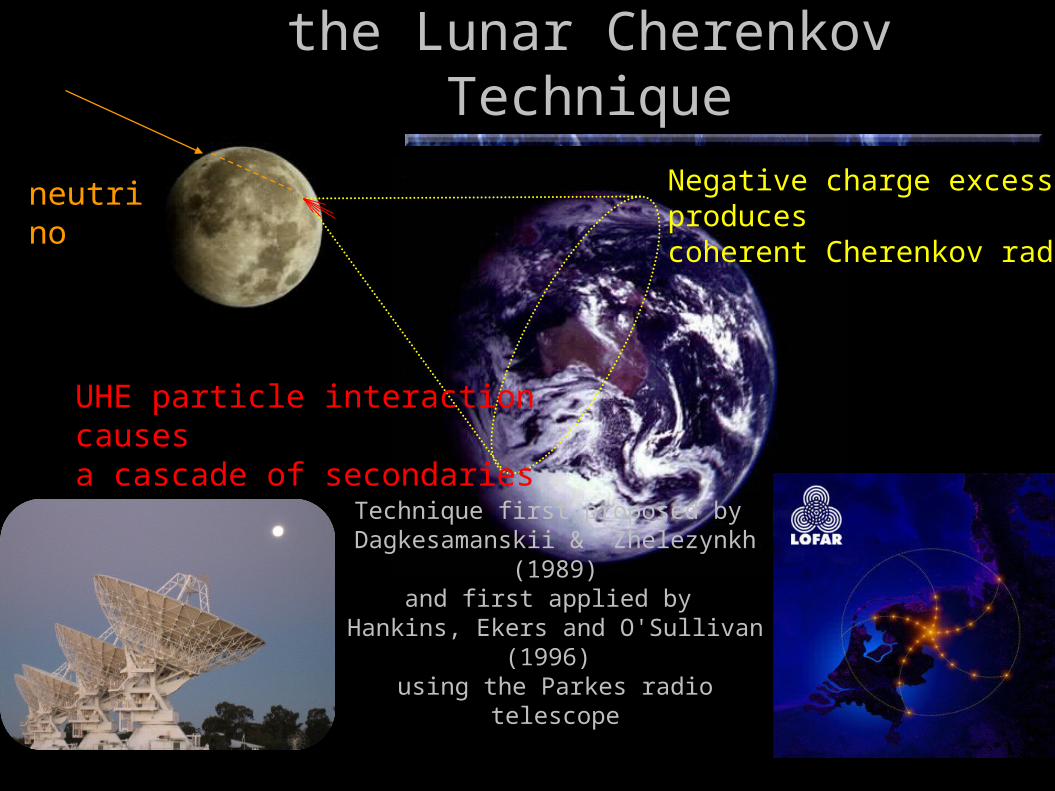
UHE Neutrino Detection using the Lunar Cherenkov Technique

neutrino Negative charge excess produces coherent Cherenkov radiation

UHE particle interaction causesa cascade of secondaries

Technique first proposed by Dagkesamanskii & Zhelezynkh (1989)

and first applied by Hankins, Ekers and O'Sullivan (1996)

using the Parkes radio telescope

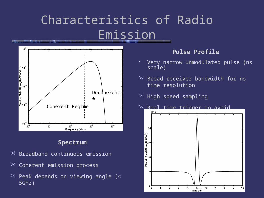
Characteristics of Radio Emission

Pulse Profile Very narrow unmodulated pulse (ns scale)

• Broad receiver bandwidth for ns time resolution

• High speed sampling

• Real time trigger to avoid excessive storage requirements

Spectrum

• Broadband continuous emission

• Coherent emission process

• Peak depends on viewing angle (< 5GHz)

Coherent Regime

Decoherence

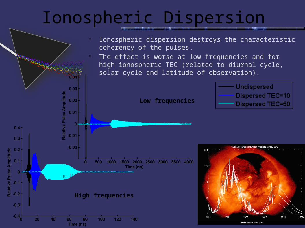
Ionospheric Dispersion

Low frequencies

High frequencies

• Ionospheric dispersion destroys the characteristic coherency of the pulses.• The effect is worse at low frequencies and for high ionospheric TEC

(related to diurnal cycle, solar cycle and latitude of observation).

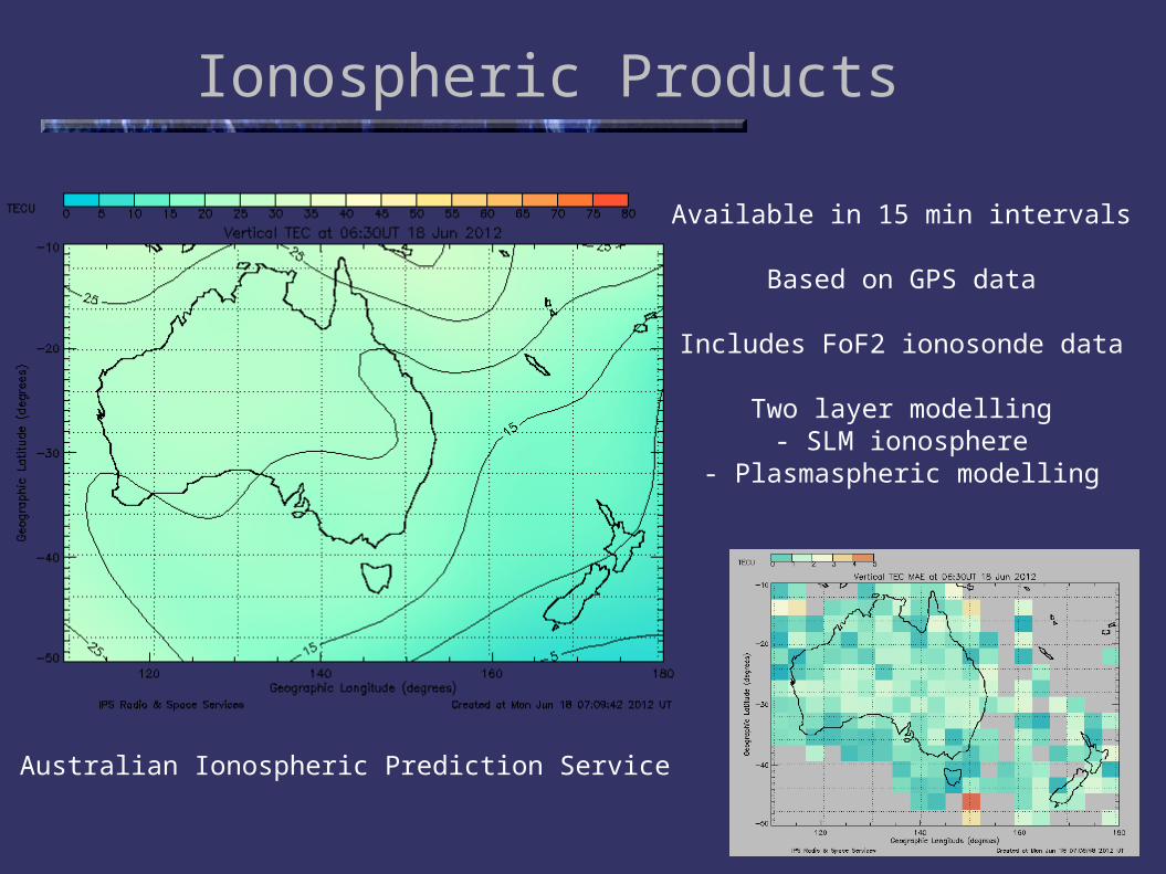
Ionospheric Products

Australian Ionospheric Prediction Service

Available in 15 min intervals

Based on GPS data

Includes FoF2 ionosonde data

Two layer modelling- SLM ionosphere

- Plasmaspheric modelling

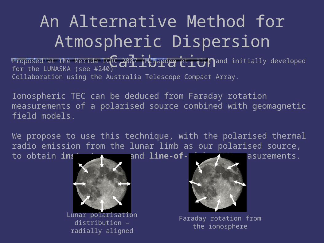
An Alternative Method for Atmospheric Dispersion Calibration

Proposed at the Merida ICRC 2007 (McFadden et. al.) and initially developed for the LUNASKA (see #240)Collaboration using the Australia Telescope Compact Array.

Ionospheric TEC can be deduced from Faraday rotation measurements of a polarised source combined with geomagnetic field models.

We propose to use this technique, with the polarised thermal radio emission from the lunar limb as our polarised source, to obtain instantaneous and line-of-sight TEC measurements.

Lunar polarisation distribution – radially aligned

Faraday rotation from the ionosphere

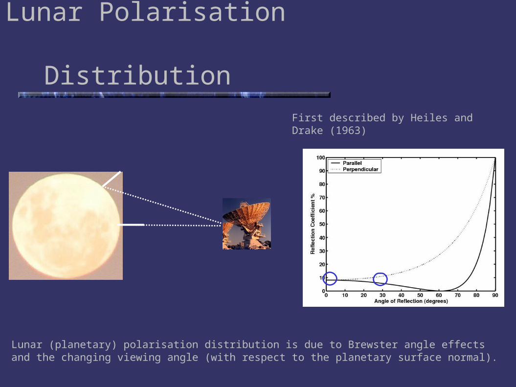
Lunar Polarisation Distribution

Lunar (planetary) polarisation distribution is due to Brewster angle effects and the changing viewing angle (with respect to the planetary surface normal).

First described by Heiles and Drake (1963)

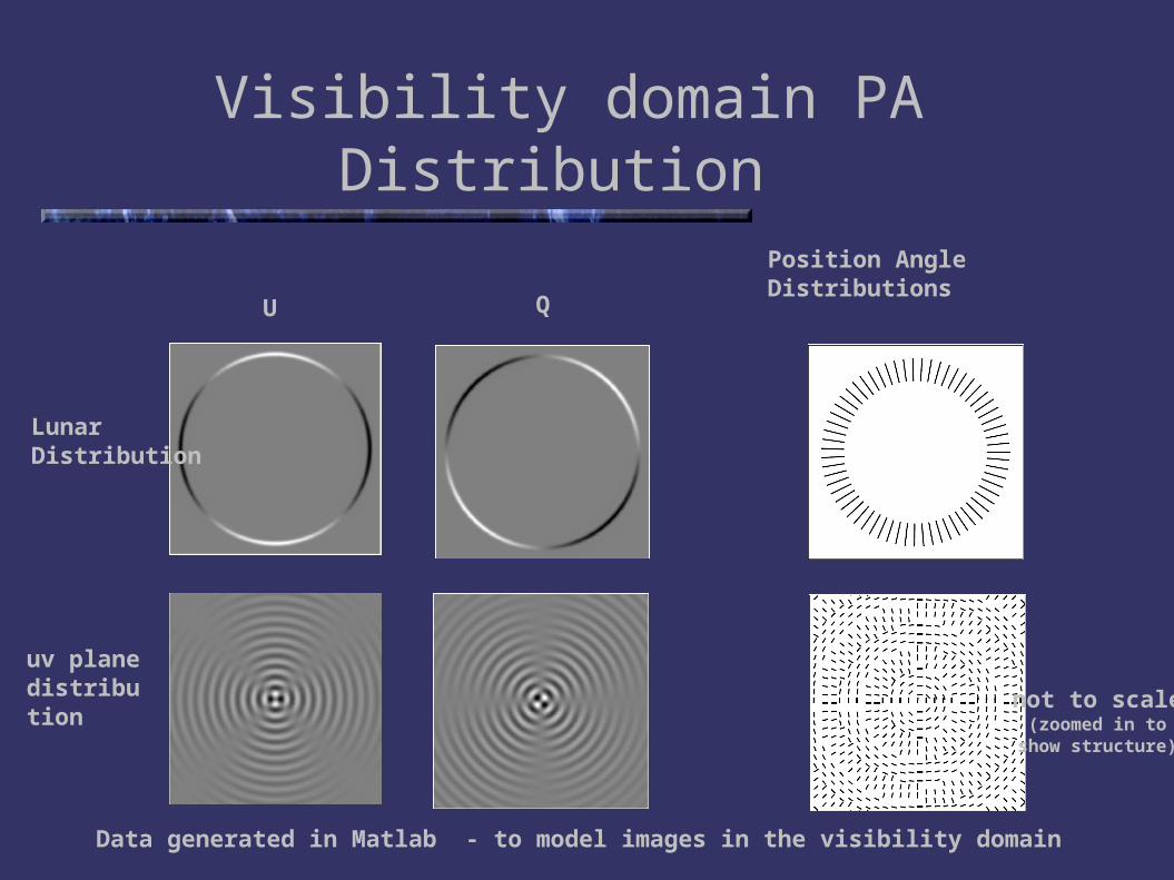
Visibility domain PA Distribution

U QPosition Angle Distributions

Lunar Distribution

uv planedistribution

Data generated in Matlab - to model images in the visibility domain

not to scale (zoomed in to show

structure)

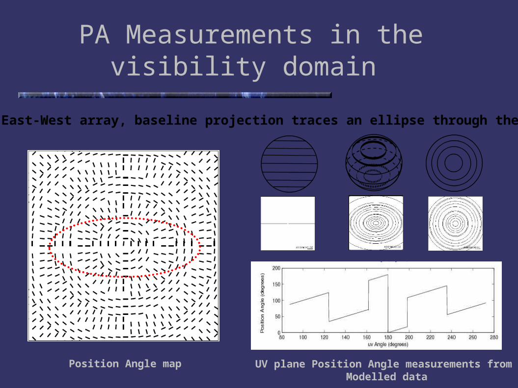
PA Measurements in the visibility domain

Position Angle map UV plane Position Angle measurements from Modelled data

For and East-West array, baseline projection traces an ellipse through the uv plane

PA Measurements in the visibility domain

Position Angle map generated in Matlab

UV plane Position Angle measurements from data modelled in Miriad

Baseline projection traces an ellipse through the uv plane

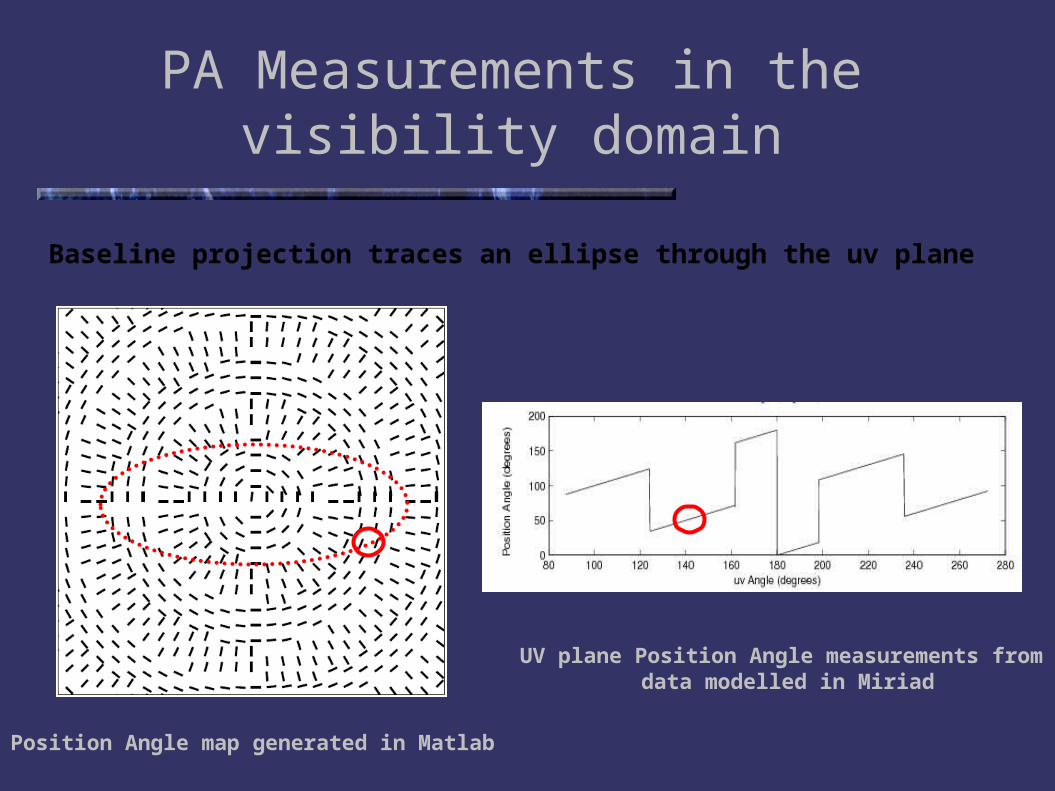
PA Measurements in the visibility domain

Position Angle map generated in Matlab

UV plane Position Angle measurements from data modelled in Miriad

Baseline projection traces an ellipse through the uv plane

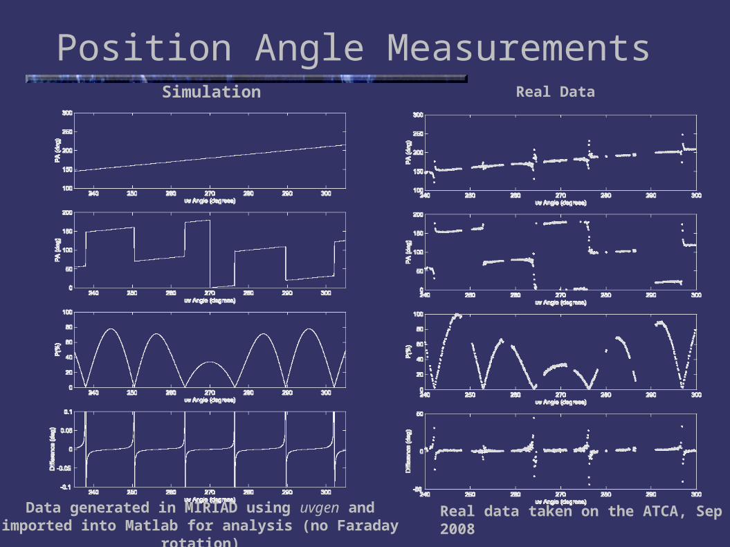
Position Angle MeasurementsSimulation Real Data

Data generated in MIRIAD using uvgen and imported into Matlab for analysis (no Faraday rotation)

Real data taken on the ATCA, Sep 2008

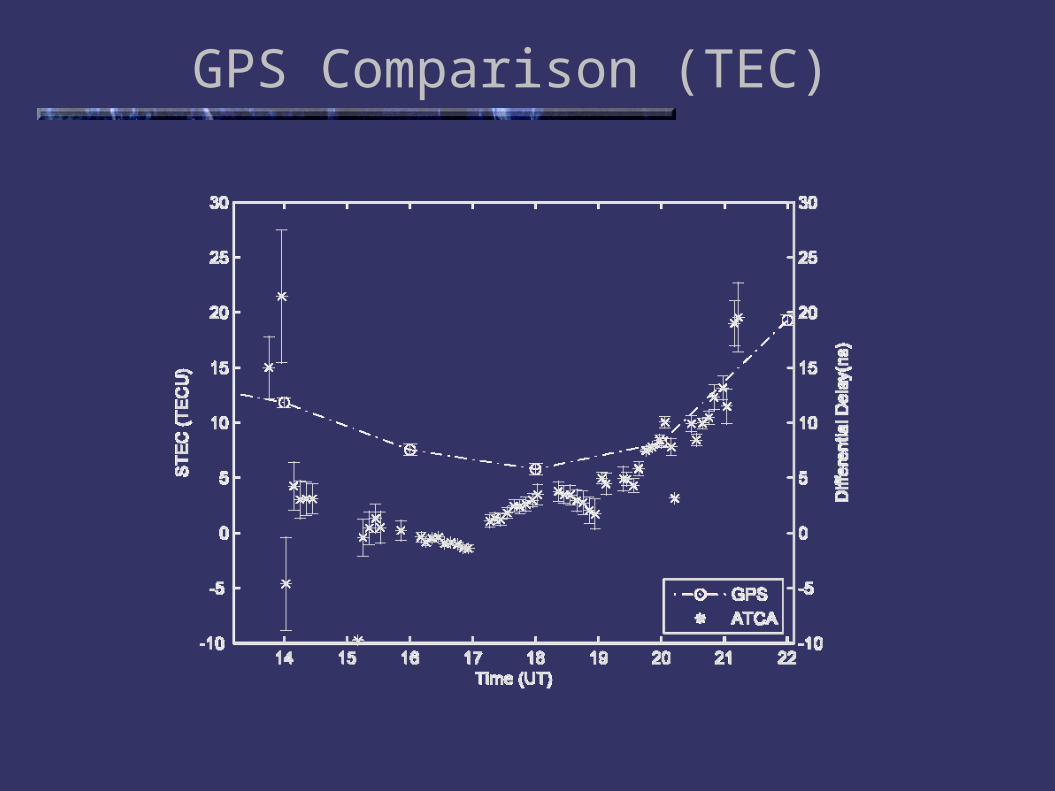
GPS Comparison (TEC)

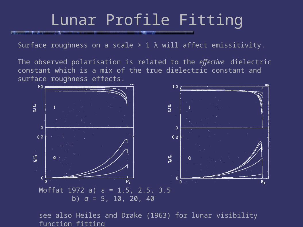
Lunar Profile Fitting

Moffat 1972 a) ε = 1.5, 2.5, 3.5 b) σ = 5, 10, 20, 40°

see also Heiles and Drake (1963) for lunar visibility function fitting

Surface roughness on a scale > 1 λ will affect emissitivity.

The observed polarisation is related to the effective dielectric constant which is a mix of the true dielectric constant and surface roughness effects.

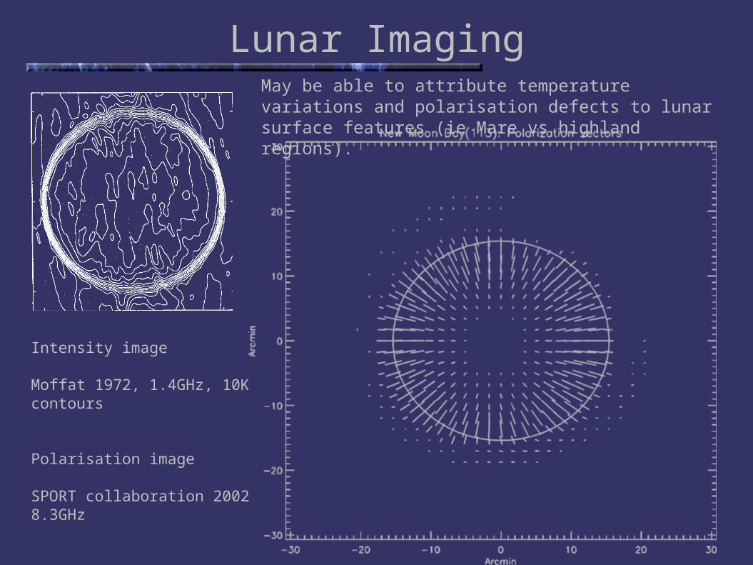
Lunar Imaging

Intensity image

Moffat 1972, 1.4GHz, 10K contours

Polarisation image

SPORT collaboration 20028.3GHz

May be able to attribute temperature variations and polarisation defects to lunar surface features (ie Mare vs highland regions).

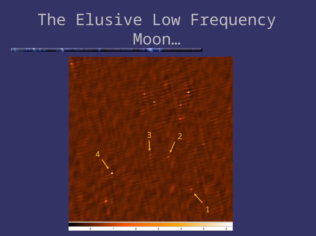
The Elusive Low Frequency Moon…

1

4

3 2

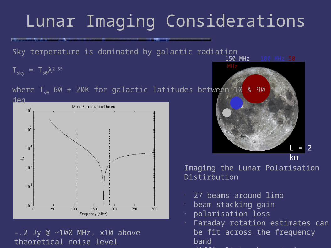
L = 2 km

150 MHz 100 MHz 50 MHz

Lunar Imaging Considerations

Sky temperature is dominated by galactic radiation

Tsky = Ts0λ2.55

where Ts0 60 ± 20K for galactic latitudes between 10 & 90 deg

-.2 Jy @ ~100 MHz, x10 above theoretical noise level

Imaging the Lunar Polarisation Distirbution

• 27 beams around limb• beam stacking gain• polarisation loss • Faraday rotation estimates can be fit across the

frequency band• difficult to characterise polarised background

emission due to phase screening effect

Future Work

• Calibration and imaging at 100MHz continues• Extend to polarisation imaging and estimate Faraday rotation• Repeat visibility domain studies with Westerbork data (1.4GHz)• Polarisation analysis to determine and map lunar surface properties at low

frequencies

Future Work

• Calibration and imaging at 100MHz continues• Extend to polarisation imaging and estimate Faraday rotation• Repeat visibility domain studies with Westerbork data (1.4GHz)• Polarisation analysis to determine and map lunar surface properties at low

frequencies

James 15 months

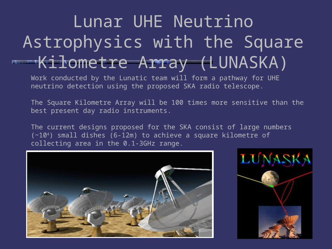
Work conducted by the Lunatic team will form a pathway for UHE neutrino detection using the proposed SKA radio telescope.

The Square Kilometre Array will be 100 times more sensitive than the best present day radio instruments.

The current designs proposed for the SKA consist of large numbers (~104) small dishes (6-12m) to achieve a square kilometre of collecting area in the 0.1-3GHz range.

Lunar UHE Neutrino Astrophysics with the Square Kilometre Array (LUNASKA)

UHE Neutrinos (~1020 eV)

Cosmic Ray energy spectrum extends from below 1010 eV to at least 1020 GeV

In the rest frame of an UHECR proton, the CMB are blue shifted to gamma ray energies and the threshold for Bethe-Heitler pair production and pion photoproduction is reached.

The origin of UHECR above this threshold (GZK cut-off) is not fully understood.

For extragalactic UHECR almost all spectral information above the GZK cut-off is lost however significant information is preserved in the spectrum of neutrinos.

UHE neutrino astronomy will be able to provide more insight into the origin of UHECR.

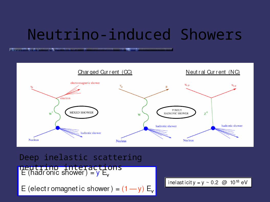
Neutrino-induced Showers

Deep inelastic scattering neutrino interactions