LUMINOSIT Y FUNCTIONS AND POINT-SOURCE PROPERTIES …

LUMINOSITY FUNCTIONS AND POINT-SOURCE PROPERTIESFROM MULTIPLE CHANDRA OBSERVATIONS OF M81

The MIT Faculty has made this article openly available. Please share how this access benefits you. Your story matters.

Citation Sell, P. H., D. Pooley, A. Zezas, S. Heinz, J. Homan, and W. H.G. Lewin. “ LUMINOSITY FUNCTIONS AND POINT-SOURCEPROPERTIES FROM MULTIPLE CHANDRA OBSERVATIONS OFM81 .” The Astrophysical Journal 735, no. 1 (June 10, 2011): 26. ©2011 The American Astronomical Society

As Published http://dx.doi.org/10.1088/0004-637x/735/1/26

Publisher IOP Publishing

Version Final published version

Citable link http://hdl.handle.net/1721.1/95652

Terms of Use Article is made available in accordance with the publisher'spolicy and may be subject to US copyright law. Please refer to thepublisher's site for terms of use.

https://libraries.mit.edu/forms/dspace-oa-articles.html

http://hdl.handle.net/1721.1/95652

The Astrophysical Journal, 735:26 (18pp), 2011 July 1 doi:10.1088/0004-637X/735/1/26C© 2011. The American Astronomical Society. All rights reserved. Printed in the U.S.A.

LUMINOSITY FUNCTIONS AND POINT-SOURCE PROPERTIES FROM MULTIPLE CHANDRAOBSERVATIONS OF M81

P. H. Sell1, D. Pooley

1,2, A. Zezas

3,4,5, S. Heinz

1, J. Homan

6, and W. H. G. Lewin

61 Department of Astronomy, University of Wisconsin-Madison, Madison, WI, USA

2 Eureka Scientific, Oakland, CA, USA3 Department of Physics, University of Crete, Heraklion, Greece

4 IESL, Foundation for Research and Technology Hellas, Heraklion, Greece5 Harvard-Smithsonian Center for Astrophysics, Cambridge, MA, USA

6 MIT Kavli Institute for Astrophysics and Space Research, Cambridge, MA, USAReceived 2010 November 22; accepted 2011 April 13; published 2011 June 10

ABSTRACT

We present an analysis of 15 Chandra observations of the nearby spiral galaxy M81 taken over the course of sixweeks in 2005 May–July. Each observation reaches a sensitivity of ∼1037 erg s−1. With these observations and oneprevious deeper Chandra observation, we compile a master source list of 265 point sources, extract and fit theirspectra, and differentiate basic populations of sources through their colors. We also carry out variability analysesof individual point sources and of X-ray luminosity functions (XLFs) in multiple regions of M81 on timescales ofdays, months, and years. We find that, despite measuring significant variability in a considerable fraction of sources,snapshot observations provide a consistent determination of the XLF of M81. We also fit the XLFs for multipleregions of M81 and, using common parameterizations, compare these luminosity functions to those of two otherspiral galaxies, M31 and the Milky Way.

Key words: galaxies: individual (M81) – X-rays: binaries – X-rays: galaxies

Online-only material: color figures, machine-readable tables

1. INTRODUCTION

Deep X-ray observations of nearby galaxies allow for thestudy of their X-ray point-source populations in considerabledetail. Previous studies of a variety of different nearby galaxieshave been able to probe these sources individually by measuringtheir spectral characteristics and luminosity variability overmany different timescales. Populations of sources can also bescrutinized by the spatial and hardness distributions of sourcesand their X-ray luminosity function (XLF).

Fabbiano & White (2006) review the X-ray point-sourcepopulations of numerous, nearby, star-forming galaxies. Oneof the most notable is M31 because of its proximity and generalsimilarities to the Milky Way. Because M31 is the closest largespiral galaxy, numerous studies have analyzed the X-ray point-source populations in great detail with past and current X-rayobservatories: Einstein (Trinchieri & Fabbiano 1991), ROSAT(Primini et al. 1993; Supper et al. 1997), Beppo Sax (Trinchieriet al. 1999), Chandra (Kong et al. 2003), and XMM-Newton(Shaw Greening et al. 2009). The two most recent observationswith XMM-Newton and Chandra, in particular, contain the bestdata yet, but only in small segments of the galaxy at a timebecause the spatial extent of the galaxy is much larger than thefields of view of these current X-ray telescopes.

In the last decade, the X-ray point-source populations ofmany other nearby, star-forming galaxies have also beenscrutinized: late-type spiral galaxies, irregular galaxies, andmerging galaxies. Not long after the launch of the Chandraand XMM-Newton space telescopes, Soria & Kong (2002),Soria & Wu (2002), and Pence et al. (2001) observed theX-ray point-source populations of M74, M83, and M101,respectively, all Sc-type spiral galaxies. More recently, theChaseM33 survey observed the X-ray point-source populationsof another Sc-type galaxy, M33 (Plucinsky et al. 2008; Williamset al. 2008), and Fridriksson et al. (2008) completed a studyof the X-ray point-source populations of a pair of galaxies,

NGC 6946 (Sc-type) and NGC 4485/4490 (an irregular galaxy).In addition, in a series of papers, Zezas et al. (2002), Zezas &Fabbiano (2002), and Zezas et al. (2006, 2007) studied the X-ray point-source population in the unique environment of themerging Antennae galaxies.

X-ray point-source populations from predominantly old stel-lar populations of early-type galaxies have also been examined.In the S0 galaxy NGC 1553, Blanton et al. (2001) found thatmost of the X-ray emission is diffuse, with 49 sources compris-ing only 30% of the light. The rest of the galaxies mentioned hereare among the many optically bright elliptical galaxies associ-ated with nearby galaxy clusters. NGC 4697 and NGC 4472(M49), two large elliptical galaxies in the Virgo cluster, havebeen observed with Chandra. Detailed analysis of NGC 4697 bySarazin et al. (2000) resolved almost all of the hard emission anda large fraction of the soft emission into 90 point sources, mostof which are expected to be low-mass X-ray binaries (LMXBs).Also, Kundu et al. (2002) and Maccarone et al. (2003) analyzedthe X-ray point-source population of NGC 4472 and found 144point sources. Lastly, a Chandra observation of the bright cen-tral galaxy in the Fornax cluster, NGC 1399, revealed 214 pointsources (Angelini et al. 2001).

From these and other studies of old stellar populations,general trends have been discerned in the X-ray populations.In the XLFs of X-ray point-source populations of ellipticalgalaxies, there is evidence for a varying break and varying slopeson either side of the break (e.g., Kim & Fabbiano 2010). Thereis also evidence for differences between the XLFs of field andcluster binaries (Fabbiano et al. 2010). Particularly prevalent inthe X-ray observations of large elliptical galaxies is the largefraction of globular cluster sources (e.g., �70% of the sourcesin NGC 1399; Angelini et al. 2001). By matching Chandraand HST observations, possible trends in the populations can beexplored (e.g., metallicity).

In these many X-ray observations of early- and late-type galaxies, these authors inspect the X-ray point-source

1

http://dx.doi.org/10.1088/0004-637X/735/1/26

The Astrophysical Journal, 735:26 (18pp), 2011 July 1 Sell et al.

populations from a variety of perspectives. Hardness ratios arefrequently calculated (albeit in a number of different ways).They are most often used to differentiate populations of sourceswithin each galaxy but have been also used to differentiate galac-tic sources from background active galactic nuclei (AGNs). Themost luminous or most unusual sources in each of the galaxiesare typically of particular interest: ultraluminous X-ray sources(ULXs), transient sources, or supersoft sources (SSSs). Theyare frequently examined in detail in terms of their spectral char-acteristics and spectral and flux variability.

When X-ray point-source populations are inspected usingXLFs of different galaxy types and stellar population ages (i.e.,actively star-forming versus relatively quiescent), considerablevariation has been observed. High-mass X-ray binary (HMXB)XLFs, which are associated with regions of current star for-mation, are typically described by straight (unbroken) powerlaws. For simplicity, we refer to these as “disk-like” XLFs inthis study. Typical cumulative slopes are ∼−0.7–1.0 for mod-erate star formation rates (SFRs; �1 M� yr−1) and ∼−0.4–0.5for higher SFRs (e.g., Kilgard et al. 2002; Grimm et al. 2002;Colbert et al. 2004). LMXB XLFs or what we refer to as “bulge-dominated” XLFs in this study are not associated with recentstar formation. These XLFs are typically described by broken orcutoff power laws (e.g., Kim & Fabbiano 2004; Gilfanov 2004)with signs of a flat low-luminosity end and a break or cutoffat a few × 1038 erg s−1, which is frequently attributed to theEddington luminosity for a neutron star. Spiral galaxies (earliertype, in particular) show mixed XLFs with contributions fromboth types of XLFs, “disk-like,” and “bulge-like.”

Developing physical models to describe the populations ofgalactic X-ray sources, which are the result of the evolutionof their stellar populations, is a daunting task. Some studieshave attempted to understand the star formation history of thesegalaxies through the use of population synthesis modeling.These complex models attempt to follow the stellar populationsthrough many evolutionary phases to the formation of theX-ray bright systems that we observe (Belczynski et al. 2008).There also exist alternate, less complex methods such as thatof Wu et al. (2003) in a previous study of M81 and White &Ghosh (1998), who construct simple birth and death rate modelsfor components of the stellar populations. However, accuratelyconstructing XLFs to low luminosities and comparing themto models is very difficult (e.g., Fragos et al. 2008), andthe information gleaned from doing this (e.g., finding andinterpreting breaks in XLFs) can be ambiguous.

Some key questions concerning XLFs remain unanswered.For example, is there a break in the XLFs of spiral galaxies atlow fluxes? Also, essentially every study of these types of X-raypoint sources has noted a wide range of levels and timescales ofboth integrated flux variability and spectral variability. However,the XLFs of galaxies are almost always characterized by asingle X-ray snapshot of the galaxy. A critical question canthen be raised: does the variability of the individual sourcessignificantly manifest itself in a variable XLF? In other words,is the XLF robust against the fluctuations of its constituents?Very large changes in the XLF over the timescales that weare probing, which are much shorter than stellar evolutiontimescales, should not be observed since this would requirecorrelated variability of many sources. However, the stabilityof XLFs has not been thoroughly investigated over the days,weeks, and years timescales.

The nearby Sb-type galaxy, M81, with multiple types ofX-ray binaries, is a key object with which to address these points

and is an excellent choice for studying the X-ray point-sourcepopulation with Chandra. Because M81 is relatively nearby ata well-determined distance (3.63 ± 0.34 Mpc; Freedman et al.1994; using the Cepheid period–luminosity relationship), wecan detect sources with faint luminosities in relatively shortexposures and calculate their luminosities accurately. However,M81 is at a large enough distance so that almost the entiregalaxy fits within the field of view of Chandra in one exposure.These facts make it easy to use Chandra to study the variabilitycharacteristics of the X-ray point-source population to relativelylow luminosities (�1037 erg s−1) in a minimum amount ofobservations.

M81’s X-ray point-source population has been scrutinizedmany times in the past. Fabbiano (1988) was the first to studythe X-ray point-source population of this galaxy with Einsteinbut was only able to detect a handful of sources. Later on,Immler & Wang (2001) studied this galaxy with ROSAT anddetected ∼5 times as many sources to fainter luminosities. Mostrecently, Tennant et al. (2001) and Swartz et al. (2003) found177 sources with Chandra in a single exposure, 17–27 of whichare expected to be background AGNs (e.g., Rosati et al. 2002).Out of these galactic sources, some are expected to be SNRs,ULXs, SSSs, or young pulsars/pulsar wind nebulae, but mostare likely LMXBs and HMXBs.

We seek to follow-up the work of Tennant et al. (2001) andSwartz et al. (2003) and to add to the understanding of thecharacteristics of the X-ray point sources and XLFs of nearbygalaxies by carrying out an observational study of the nearbygalaxy M81. We use a set of 16 Chandra observations of M81that explore variability on timescales of days, weeks, and years.We also use these observations to make the most complete studyof M81’s X-ray point-source population to date.

In Section 2, we lay out the observations and data reductionprocedures. Then, in Section 3, we discuss the creation of ourpoint-source catalogs. In Sections 4 and 5, we present hardnessratios and discuss the individual variability of the point-sourcepopulation, respectively. Following this, we construct XLFs inSection 6. Then, in Section 7, we compare our results withM31 and the Milky Way. Finally, in Section 8, we summarizeour results and state our conclusions. For all of our analysesthroughout this work, we use the energy range of 0.5–8.0 keV(e.g., fluxes, luminosities), unless otherwise noted.

2. OBSERVATIONS AND DATA REDUCTION

We present 15 Chandra observations of M81 (ObsIDs 5935-5949) taken specifically to explore XLF and individual point-source variability. For our analysis, we include an additionalobservation from the Chandra archive (ObsID 735; Tennantet al. 2001; Swartz et al. 2003) to provide a longer baseline formeasuring variability (see Table 1). All 16 observations weretaken with the Advanced CCD Imaging Spectrometer (ACIS;Garmire et al. 2003) in Timed Exposure mode with a frame timeof 3.2 s and the aimpoint on the default location of the S3 chip.The data were telemetered to the ground in faint mode.

We analyze all of these observations using the CIAO softwareprovided by the Chandra X-ray Center as well as the IDL-basedACIS Extract program version 2008-03-04 (AE; Broos et al.2010). We ignore the ACIS-I chips for the entire analysis forthree primary reasons: (1) the observations were purposely takento line-up the galaxy on the ACIS-S chips so that any sourcesfound on the ACIS-I chips are far less-likely to be associatedwith M81, (2) point-source extractions for sources on chips I2or I3 become very difficult because the CALDB PSF library

2


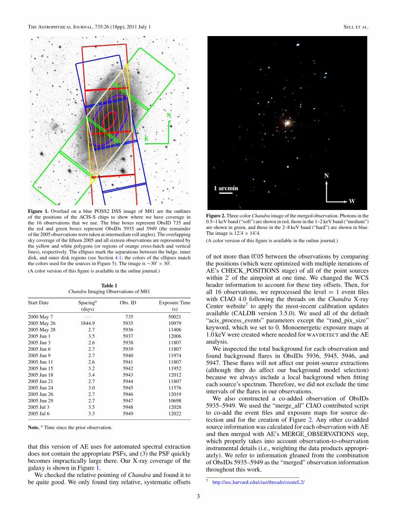
Figure 1. Overlaid on a blue POSS2 DSS image of M81 are the outlinesof the positions of the ACIS-S chips to show where we have coverage inthe 16 observations that we use. The blue boxes represent ObsID 735 andthe red and green boxes represent ObsIDs 5935 and 5949 (the remainderof the 2005 observations were taken at intermediate roll angles). The overlappingsky coverage of the fifteen 2005 and all sixteen observations are represented bythe yellow and white polygons (or regions of orange cross-hatch and verticallines), respectively. The ellipses mark the separations between the bulge, innerdisk, and outer disk regions (see Section 4.1; the colors of the ellipses matchthe colors used for the sources in Figure 5). The image is ∼30′ × 30′.(A color version of this figure is available in the online journal.)

Table 1Chandra Imaging Observations of M81

Start Date Spacinga Obs. ID Exposure Time(days) (s)

2000 May 7 · · · 735 500212005 May 26 1844.9 5935 109792005 May 28 2.7 5936 114062005 Jun 1 3.5 5937 120062005 Jun 3 2.6 5938 118072005 Jun 6 2.7 5939 118072005 Jun 9 2.7 5940 119742005 Jun 11 2.6 5941 118072005 Jun 15 3.2 5942 119522005 Jun 18 3.4 5943 120122005 Jun 21 2.7 5944 118072005 Jun 24 3.0 5945 115762005 Jun 26 2.7 5946 120192005 Jun 29 2.7 5947 106982005 Jul 3 3.5 5948 120282005 Jul 6 3.3 5949 12022

Note. a Time since the prior observation.

that this version of AE uses for automated spectral extractiondoes not contain the appropriate PSFs, and (3) the PSF quicklybecomes impractically large there. Our X-ray coverage of thegalaxy is shown in Figure 1.

We checked the relative pointing of Chandra and found it tobe quite good. We only found tiny relative, systematic offsets

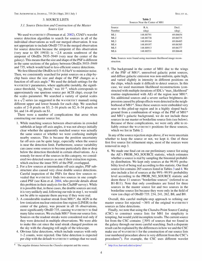
Figure 2. Three-color Chandra image of the merged observation. Photons in the0.5–1 keV band (“soft”) are shown in red, those in the 1–2 keV band (“medium”)are shown in green, and those in the 2–8 keV band (“hard”) are shown in blue.The image is 12.′4 × 14.′4.

(A color version of this figure is available in the online journal.)

of not more than 0.′′05 between the observations by comparingthe positions (which were optimized with multiple iterations ofAE’s CHECK_POSITIONS stage) of all of the point sourceswithin 2′ of the aimpoint at one time. We changed the WCSheader information to account for these tiny offsets. Then, forall 16 observations, we reprocessed the level = 1 event fileswith CIAO 4.0 following the threads on the Chandra X-rayCenter website7 to apply the most-recent calibration updatesavailable (CALDB version 3.5.0). We used all of the default“acis_process_events” parameters except the “rand_pix_size”keyword, which we set to 0. Monoenergetic exposure maps at1.0 keV were created where needed for wavdetect and the AEanalysis.

We inspected the total background for each observation andfound background flares in ObsIDs 5936, 5945, 5946, and5947. These flares will not affect our point-source extractions(although they do affect our background model selection)because we always include a local background when fittingeach source’s spectrum. Therefore, we did not exclude the timeintervals of the flares in our observations.

We also constructed a co-added observation of ObsIDs5935–5949. We used the “merge_all” CIAO contributed scriptto co-add the event files and exposure maps for source de-tection and for the creation of Figure 2. Any other co-addedsource information was calculated for each observation with AEand then merged with AE’s MERGE_OBSERVATIONS step,which properly takes into account observation-to-observationinstrumental details (i.e., weighting the data products appropri-ately). We refer to information gleaned from the combinationof ObsIDs 5935–5949 as the “merged” observation informationthroughout this work.

7 http://asc.harvard.edu/ciao/threads/createL2/

3

http://asc.harvard.edu/ciao/threads/createL2/


3. SOURCE LISTS

3.1. Source Detection and Construction of the MasterSource List

We used wavdetect (Freeman et al. 2002), CIAO’s waveletsource detection algorithm to search for sources in all of theindividual observations as well our merged observation. It wasnot appropriate to include ObsID 735 in the merged observationfor source detection because the aimpoint of this observation(very near to SN 1993J) is ∼2.8 arcmin southwest of theaimpoint of ObsIDs 5935–5949 (very near the center of thegalaxy). This means that the size and shape of the PSF is differentin the same sections of the galaxy between ObsIDs 5935–5949and 735, which would lead to less-efficient source detections.

We first filtered the ObsIDs to 0.5–6.0 keV to minimize noise.Then, we consistently searched for point sources on a chip-by-chip basis since the size and shape of the PSF changes as afunction of off-axis angle.8 We used the default settings for thewavdetect parameters, where applicable (notably, the signifi-cance threshold, “sig_thresh,” was 10−6, which corresponds toapproximately one spurious source per ACIS chip), except forthe scales parameter. We searched a variety of spatial scalesin a

√2 series (as suggested in the wavdetect manual) using

different upper and lower bounds for each chip. We searchedscales of 2–8 pixels on S3, 2–16 pixels on S2, 6–34 pixels onS4, and 14–40 pixels on S1.

There were a number of complications that arose whenconstructing our master source list.

1. While matching sources between observations in crowdedsubfields at large off-axis angles, it was not always initiallyclear whether the apparently matched source was actuallythe same source or whether we were confusing multiplenearby sources. This is because the position uncertaintyfar off-axis can be quite large, especially when the sourceis near the detection limit. Furthermore, source variabilitycan cause some sources to become particularly dim or dropbelow the detection threshold in certain observations. As aremedy for most of the sources in this category, we consid-ered two detected sources as one if their extraction regions,which enclose the inner 50% of the PSF, overlapped.

2. For a few sources at intermediate off-axis angles, PSF sub-structure also caused very close double source detections.Careful inspection of the PSFs for these few sources re-vealed that wavdetect finds two sources in one compli-cated PSF (see Kim et al. 2004, who provide details aboutthis problem in their analysis for the ChaMP survey). Whileit is possible that, in these cases, the double sources are real,it is very unlikely and, following our rule in step 1, we wouldnot be able to separate them anyway if they were real.

3. A considerable readout streak from M81*, the AGN in thelow-ionization nuclear emission-line region (LINER) in thecenter of the galaxy, was present in all 16 observations,most significantly ObsID 735, causing wavdetect to findmany false sources. We exclude M81* from our source lists.Sources on the readout streaks were considered real only ifthey were detected in multiple observations. We were ableto make this cut since the read streak changed position onthe sky with the changing roll angle of the telescope.

4. Obvious false detections, which include sources with only1–2 counts, were rejected. One false detection is expectedper chip with the default wavdetect settings that we used.

8 The angular distance between the Chandra aimpoint and the source.

Table 2Sources Near the Center of M81

Source R.A. Decl.Number (deg) (deg)

ML1 148.88791 69.06654ML2 148.88738 69.06575ML3 148.89164 69.06485ML4 148.89197 69.06385ML5 148.88913 69.06377ML6 148.88531 69.06648

Note. Sources were found using maximum likelihood image recon-struction.

5. The background in the center of M81 due to the wingsof the PSF of M81*, unresolved galactic point sources,and diffuse galactic emission was non-uniform, quite high,and varied slightly in intensity in different positions onthe chips, which made it difficult to detect sources. In thiscase, we used maximum likelihood reconstructions (con-structed with multiple iterations of IDL’s “max_likelihood”routine–implemented with AE) of the region near M81*.Six additional sources and a severe surface brightness de-pression caused by pileup effects were detected in the neigh-borhood of M81*. Since these sources were embedded verynear to this piled-up region and in a highly sloped back-ground from a combination of wings of the PSF of M81*and M81’s galactic background, we do not include thesesources in our master or borderline source lists (see below).Because of these complications, we were only able to re-liably extract the wavdetect positions for these sources,which we list in Table 2.

In any of the source rejection steps above, if we were uncertainwhether to keep the source or not, we kept it. Out of thesefirst five source list refinement steps, most of the sources wereremoved in step 3.

6. We made one final cut on our preliminary source list usingthe AE’s PROB_NO_SOURCE statistic, which estimateswhether a source is real by sampling the binomial probabil-ity distribution. We kept only sources at the 99.9% proba-bility level of being real according to this statistic. Our finalsource list contains 265 sources listed in Tables 3 and 4. Wealso include a list of sources at the 99%–99.9% probabilitylevel according to the PROB_NO_SOURCE statistic anddeem these 11 sources “borderline sources” (referred to asB1-B11). Note that only coordinates are listed for threesources in the master source list and two sources in theborderline source list because they were only in the field ofview (on chip) of ObsID 735: 234, 241, 262, B8, and B9.

Overall, this careful multiple-step approach to refining ourmaster source list rejected ∼36% of the original wavdetect

sources as false detections.Finally, we note that using the Chandra Point Source Catalog

(CSC) to construct source lists for M81 for simplicity istempting, but would yield incomplete results. The current sourcelist from the CSC contains �50% of sources that we found inthe galaxy through our more careful searching. Such a disparateresult can be explained by the differences in how we and the CSCmake use of wavdetect for the construction of our source lists(our numbered procedure above is very different from the CSC’sprocedures9). For example, the CSC uses different wavelet

9 http://cxc.harvard.edu/csc/proc/

4

http://cxc.harvard.edu/csc/proc/


Table 3Merged Extraction Data of Sources in the Master and Borderline Source Lists

Src R.A. Decl. Avg OAA Tot Src Tot Bkg Soft Net Medium Net Hard Net PSF % Var Stat Var Obs Var StatNumber (deg) (deg) (arcmin) (counts) (counts) (counts) (counts) (counts) 5935–5949 5935–5949 merged-735

1 149.076036 68.822964 14.527 936 744.5 67.6+19.3−18.3 93.4+15.1

−14.1 31.6+26.8−25.8 90.0 1.78 5940.5945 1.44

2 149.113274 68.868505 12.209 807 591.2 51.3+18.0−16.9 99.5+14.6

−13.5 65.0+25.0−23.9 90.1 2.36 5937.5946 2.09

3 149.172497 68.888582 11.692 519 359.7 24.8+15.0−14.0 82.1+12.8

−11.7 53.4+19.9−18.9 90.0 3.18 5940.5945 2.49

4 149.162574 68.904939 10.738 150 105.9 5.1+7.9−6.8 13.7+6.5

−5.5 25.3+11.6−10.5 90.3 2.24 5942.5947 2.05

5 149.256021 68.916976 11.372 655 151.4 145.0+21.9−20.9 250.3+17.7

−16.6 108.2+16.8−15.7 90.3 4.55 5945.5948 3.59

6 148.776150 68.741468 19.003 207 129.0 17.7+10.2−9.1 33.1+8.4

−7.3 28.2+12.7−11.6 90.8 3.90 5937.5938 3.43

7 149.148898 68.762466 18.458 1481 1357.4 17.8+21.4−20.4 70.5+17.6

−16.5 35.3+35.1−34.1 90.1 2.99 5938.5948 2.66

8 149.378579 68.818487 17.638 981 758.1 62.7+19.8−18.8 108.8+16.1

−15.1 51.4+27.3−26.3 90.2 3.35 5947.5948 2.95

9 149.057171 68.956754 6.933 185 9.9 92.7+13.9−12.8 69.3+9.5

−8.4 13.1+5.6−4.4 69.5 1.95 5944.5948 1.44

10 148.799329 68.963358 5.865 46 8.8 6.0+5.9−4.8 14.4+5.1

−4.0 16.8+5.9−4.8 90.2 1.14 5936.5941 0.99

Notes. Column 1: source number. A “B” before the number refers to a borderline source not part of the master source list. Columns 2 and 3: right ascension anddeclination of the source in J2000 decimal degrees coordinates. Column 4: “Average OAA” = “Average Off-Axis Angle,” the average angle on the sky between thesource and the aimpoint of the observation in the merged observation. Column 5: “Tot Src Counts” refers to the number of source counts extracted in all of the sourceregions in observations 5935–5949. Column 6: “Tot Bkg Counts” refers to the number of background counts expected in the source region based on the nearby annularmerged background extraction. Columns 7, 8 and 9: soft (0.5–1 keV), medium (1–2 keV), and hard (2–8 keV) background-subracted counts with Gehrels (1986) errors.Column 10: “PSF %” is the average fraction of the point-spread function enclosed by the source extraction region. Column 11: “Var Stat” is the variability statisticas defined in Equation (1) between ObsIDs 5935–5949. Column 12: “Var Obs” are the two observations corresponding to Column 11. Column 12: “Var Stat” is thevariability statistic as defined in Equation (1) between the merged observation and ObsID 735. Abbreviations of table values: “OC” = “Off Chip.” “NA” = “NotApplicable/Available.” This occurs in the case of the variability statistic when the source is only on the chips in one of ObsIDs 5935–5949 or off the ObsID 735 chips.

(This table is available in its entirety in a machine-readable form in the online journal. A portion is shown here for guidance regarding its form and content.)

Table 4Merged Fit Data of Sources in the Master and Borderline Source Lists

Src Model Γ or Model NH C-Stat (DOF) Luminosity CommentsNumber Type kT Normalization (1022 cm−2) (1037 erg s−1)

1 plaw 2.36+0.67−0.56 4.35e-06+2.14e−06

−1.42e−06 0.14+0.14−0.24 1231.6 (1014) 1.92+0.41

−0.41

2 plaw 1.29+0.39−0.33 2.54e-06+9.80e−07

−6.34e−07 0.07+0.11−0.07 1156.9 (1014) 3.24+0.56

−0.56 POC 5937, 5938

3 plaw 1.54+0.52−0.44 3.62e-06+2.12e−06

−1.21e−06 0.27+0.20−0.46 1073.4 (1014) 3.08+0.57

−0.57 POC 5939, 5940

4 plaw 2.53+3.01−2.44 4.79e-06+1.38e−04

−4.53e−06 1.89+2.64−1.89 1064.8 (1014) 0.77+0.28

−0.28 POC 5939, 5940

5 plaw 2.14+0.22−0.21 2.31e-05+4.36e−06

−3.53e−06 0.16+0.06−0.05 1127.9 (1014) 11.61+0.65

−0.65

6 plaw 1.65+0.75−0.63 1.26e-05+1.11e−05

−5.54e−06 0.19+0.25−0.19 1036.2 (1014) 9.89+2.32

−2.32 S61; POC 5937, 5938 5938

7 bbod 0.80+0.27−0.18 1.84e-07+9.48e−08

−6.03e−08 0.04+0.21NA 1436.4 (1014) 2.33+1.00

−1.00 POC 5937, 5938, 5941–5946 5941–5946

8 plaw 1.89+0.58−0.49 1.09e-05+5.20e−06

−3.32e−06 0.14+0.14−0.26 1301.6 (1014) 7.03+1.31

−1.31 POC 5945

9 bbod 0.19+0.04−0.01 1.91e-07+2.84e−08

−5.92e−08 0.04+0.02NA 870.9 (1014) 1.49+0.12

−0.12 VC 41; POC 5935 5935

10 plaw 1.22+0.37−0.46 5.32e-07+1.58e−07

−1.98e−07 0.04+0.06NA 756.3 (1014) 0.75+0.24

−0.21 S71

Notes. Column 1: source number. A “B” before the number refers to a borderline source not part of the master source list. Column 2: The model used for fitting thespectrum (“plaw” = power law and “bbod” = blackbody). Column 3: Γ = Powerlaw Index, kT = Blackbody Temperature (keV) of the best-fit model. Column 4:“Model Normalization” is the model normalization in units of photons keV−1 cm−2 s−1 at 1 keV for the power-law model and L39/(D10)2, where L39 is the sourceluminosity in units of 1039 erg s−1 and D10 is the distance to the source in units of 10 kpc for the blackbody model. Column 5: The best-fit column density for the sourcewhich includes galactic foreground and intrinsic source absorption. A value is “0.04” indicates that the best-fit is on the galactic foreground minimum column density(the lower bound will then be “NA”). Column 6: “C-stat (DOF)” is the total best-fit C-statistic and number of degrees of freedom for the source and background modelstogether. Column 7: The 0.5–8.0 keV luminosity calculated from the best fit model. The uncertainties are estimated by scaling the luminosity by the uncertainty in thecounts, which was calculated from the 90% Bayesian confidence intervals, (Kraft et al. 1991). Column 8: Other details about the source extraction. Abbreviations oftable values: “OC” = “Off Chip.” “NA” = “Not Applicable/Available.” This occurs when: in the case of source 62, the model is too complicated to be listed in thetable; Sherpa fails to find the confidence interval; the source has zero flux so that Γ or kT is not defined. An “f” indicates that the parameter was frozen during thespectral fitting. “RS ObsID” indicates that the source was on the readout streak in the specified ObsID. “POC ObsID” indicates that the source was partially off of thechip in the specified ObsID. “S#” indicates the Swartz source number that this source is matched to. “VC #” indicates that the source was very close to another source.a Sherpa’s JD pileup model (Davis 2001) was used in addition to the power-law fit.b See Swartz et al. (2003) for model parameters.

(This table is available in its entirety in a machine-readable form in the online journal. A portion is shown here for guidance regarding its form and content.)

scales, energy filtering, blocking, and significance thresholds.The most important difference to the overall process is that we

have stacked our 15 new observations, revealing a multitude ofadditional, faint sources.

5


3.2. Point-source Extraction with ACIS Extract

We used AE for the extraction of the source and backgroundspectra. One of the primary reasons that we use AE (as opposedto other CIAO tools such as psextract) is that AE calculatesthe size, shape, and position of each extraction region, andit calculates the auxiliary response file (ARF)10 taking intoaccount the PSF fraction enclosed in the region as a function ofenergy. We also use AE to refine the positions beyond the initialwavdetect estimates and calculate some useful statistics andphotometry.

We briefly lay out the point-source extraction process here.First, we constructed regions to match the PSF retreived fromthe CALDB library and that enclose a prescribed percentage ofthe PSF (90% default unless it needed to be adjusted to as lowas 50% for nearby sources relative to the size of the PSF). Thenfor each point source, we extracted the source events withinthe PSF-matched region and a representative background in anannular region centered on the point source.

With this information, AE then provides new position esti-mates for each of the sources. We refined the positions of thesources according to the prescriptions in the AE manual. Forsources that were �5′ from the aimpoint, we used the meanevent position, and, for sources that were >5′ from the aim-point, we used the correlation position. The latter position iscalculated automatically by AE, by correlating the neighbor-hood around the source (not just the extracted counts) with thesource’s PSF. Since the positions of some of the sources (es-pecially the fainter ones) take time to converge, we ran thesefirst few steps a minimum of five times. This provides us withvery accurate source positions, useful for comparing to obser-vations taken with other telescopes and provides accurate fluxestimates.

Lastly, we extracted the spectra for each source and its lo-cal background, which included the creation of the ARF andRMF (redistribution matrix file)11 files for fitting the spectra.AE implements rules so that the background is always wellconstrained. At minimum, the background spectrum must al-ways have at least 100 counts and a ratio of the photomet-ric errors of the source to background of at least 4.0 (so thatthe error in the background does not dominate the total er-ror). These constraints on the background extraction yieldeda median background radius of 76 sky pixels with >99% ofthe sources having radii less than ∼200 sky pixels and < 1%of the sources farthest off-axis having radii of ∼200–500 skypixels.

3.3. Spectral Fitting and Source Properties

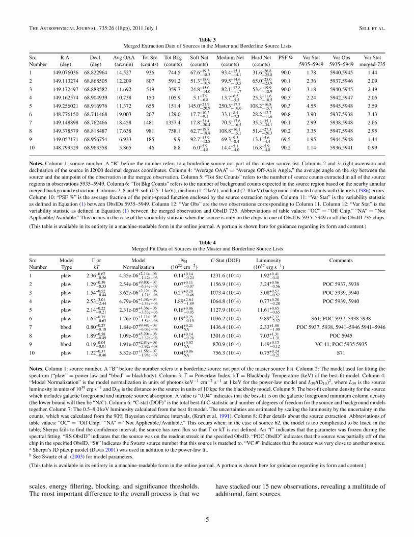
To estimate the energy fluxes and other source properties, wefit the source and background spectrum of each source in eachobservation (∼4000 spectra, most fit using automated methodsdetailed below). We tested an alternate method of estimatingfluxes by using a single count-rate-to-flux conversion factor. Wefound that this would have led us to calculate different sourcefluxes by factors of order unity or less (see Figure 3; see alsoSection 7.2 for a brief discussion of this effect with regard tothe XLFs). We jointly fit the unbinned source and backgroundspectrum of each source in each observation12 in Sherpa

10 http://cxc.harvard.edu/ciao/dictionary/arf.html11 http://cxc.harvard.edu/ciao/dictionary/rmf.html12 For each source in each observation, the source and scaled backgroundspectrum fits were added together (the background was not subtracted), andthen the total spectral fit was minimized.

Figure 3. Source hardness as a function of conversion factor from counts to ergfor sources in our merged master source list. The estimated source flux will bebiased if a single conversion factor is used to convert counts to energy flux units.The vertical line of points near 3.3 represents the spectral fits where the photonindex was frozen to 1.7 and NH was frozen to or floated to the minimum valuein the direction of M81. The points only extend ∼1–11 on the x-axis because ofthe constraints imposed on the fit parameters, which are laid out in Section 3.3.The hardness ratio for a photon index of 1.7 and a column density equal tothe Galactic column density in the direction of M81 is −0.39 ((H−S)/T). H:2–8 keV; S: 0.5–2 keV, T: 0.5–8 keV.

(Freeman et al. 2001) using the C-statistic, which is similarto the Cash (1979) statistic but with an approximate goodness-of-fit measure, and the Powell minimization algorithm.

Since almost all of the sources have too few countsto constrain many of their source properties and since weare mainly interested in estimating accurate fluxes, we be-gan by fitting the source and background spectra for eachsource in each observation with absorbed power-law models(xswabs × xspowerlaw).13 We initially used the defaultparameter boundaries (xswabs.nH = [0.01,10] (1022 cm−2),xspowerlaw.PhoIndx = [−3,10], xspowerlaw.norm is es-timated from the data) in Sherpa in all cases except one. Wealways constrained the hydrogen column density to be at leastthat of the Milky Way in the direction of M81, 4.2 × 1020 cm−2

(Dickey & Lockman 1990).Since degeneracies in the fit parameters will frequently arise

for very faint sources, we followed a specialized scheme forthese sources based on the number of counts in the sourceextraction region. If we extracted less than 5 counts (0.5–8 keV)for a source, the power-law index and the hydrogen columndensity for the fit were frozen to 1.7 and the Galactic value,respectively. If we extracted more than 5 but less than 26 counts(0.5–8 keV), we froze only the power-law index to 1.7 and letthe hydrogen column density float, although, in this case, it wasalways poorly constrained. For all other sources with more than26 counts (0.5–8 keV), we allowed all fit parameters to float.

Following these rules, we obtained reasonable fits for most ofthe sources. However, some of the individual-observation sourcespectra (∼17%) did not have acceptable fits using these rulesalone. First, the background spectra were not always well fit by asingle absorbed power-law model. The merged spectra revealedthat, when well-sampled, background spectra were always quitecomplicated. These complications exhibited themselves some-times in the individual observation source spectra. For the cases

13 Use of the xsphabs absorption model instead does not make a significantdifference to the fits.

6

http://cxc.harvard.edu/ciao/dictionary/arf.html

http://cxc.harvard.edu/ciao/dictionary/rmf.html


where the reduced goodness-of-fit statistic for the backgroundspectrum was �0.9,14 a more complicated background model,two power laws and a blackbody (xswabs × (xspowerlaw +xspowerlaw + xsbbody)) was used to achieve a good fit. Thisad hoc combination of models is only used to model the shapeof the background spectra.

Second, there were some sources (�4% of the fits) in whichthe best-fit hydrogen column density of the source was foundat the maximum of the parameter space, 1023 cm−2. Since thesimple absorption model does not account for multiple photonscatterings through a Compton-thick medium and we did notconsider other absorption models for our spectral fitting, werefit the spectra using a maximum hydrogen column density of1024 cm−2, which allowed for reasonable spectral fits for mostof these sources. However, there were still a small subset ofsources (�1% of the fits) with 5–25 counts where the best-fithydrogen column densities were at 1024 cm−2. For these fewsources, we allowed the power-law photon index, Γ, to float.This led to reasonable fits for these sources.

Third, there were sources with best-fit power-law indices upto 10, the maximum parameter space boundary. For these softsources with Γ > 3 (�3%), we changed the source modelto a simple thermal (xsbbody) model and achieved good fits(C-statistic � 1 with kT< 1 keV). Our change in spectral modelhere does not imply that there are not sources that could be wellfit by this model with temperatures in excess of 1 keV. Given thelimited number of source counts for most sources, we expect thatsuch sources were well fit by the absorbed power-law model.This only implies that there were sources that could not be wellfit by the absorbed power-law model within a reasonable rangeof photon indices because their spectra were too soft. This resultindicates that we cannot differentiate these models for most ofour sources that are not very soft. This is acceptable since ourgoal is not to differentiate source models. These comments alsoapply to the merged spectra that are mentioned below.

Fourth, a very small number of sources (�1%) had Γ < 0 orhad spectra such that Sherpa could not find a reasonable localminimum and frequently ran into parameter space boundaries.These were generally sources that had only a few counts andwere located in regions where the background spectrum wascomplicated. In these cases, the software had to be manuallyguided until a reasonable fit was found.

In summary, we allowed for fairly liberal upper and lowerbounds for the fit parameters because there are a wide range ofdifferent types of sources in our sample (e.g., LMXBs, HMXBs,SNRs, SSSs, ULXs, background AGNs, etc.). After consider-able experimentation and iteration, the following constraintswere imposed on our spectral fitting process.

1. We required the reduced goodness-of-fit statistic for thesource to be better than 1.2.

2. We required the reduced goodness-of-fit statistic for thebackground to be better than 0.9 for sources within 7 arcminof the aimpoint and better than 1.4 for sources farther off-axis than 7 arcmin.

3. The source absorption, NH, must be less than 1024 cm−2

(the Compton-thick limit).4. No sources can be very close to or stuck at parameter space

boundaries.5. The source power-law fits cannot have a photon index

greater than 3 or less than 0.

14 The cutoff value for the goodness-of-fit statistic is smaller than 1 becausethis reduced statistic was typically underestimated near ∼0.5.

6. The blackbody (thermal) fits were specifically implementedonly for very soft sources and do not have kT greater than1 keV.

At the end of the fitting process, all fits abided by these rules.Out of all source fits in each of the 16 observations, two

sources in ObsID 735 required special attention with the use ofmore complicated models. First, the brightest ULX (source 21)was the only source that suffered from significant pileup and,therefore, Sherpa’s JD pileup model (Davis 2001) was used inaddition to the power-law fit. The second source, SN1993J (theaim of ObsID 735), was fit by two low-temperature absorbedthermal emission-line (vmekal) components. Since care hasalready been taken in fitting these sources (Swartz et al. 2003),we used these models.

We also fit the source spectra of ObsIDs 5935–5949, themerged observation, to better understand the properties of eachsource. We did not include the ObsID 735 in the merged spectrabecause the ARF changes significantly and there appears to bespectral variability in at least a few sources (see Section 5.2).We fit the merged source spectra with simple absorbed power-law models as above. We found that 219 of the 262 sourceswere well-fit by this method (CSTAT � 1). Again, two sources(the brightest ULX and SN1993J) were fit with special models,as described in the previous paragraph. The remaining sourceswere better fit by simple blackbody (thermal) models. Almost allof the sources better fit with the simple thermal model also hadhardness ratios indicative of thermal SNR or SSS populations(see Section 4). In all cases, the background was poorly fit bya single absorbed power law. We used the more complicatedbackground model expressed above, which achieved good fits.

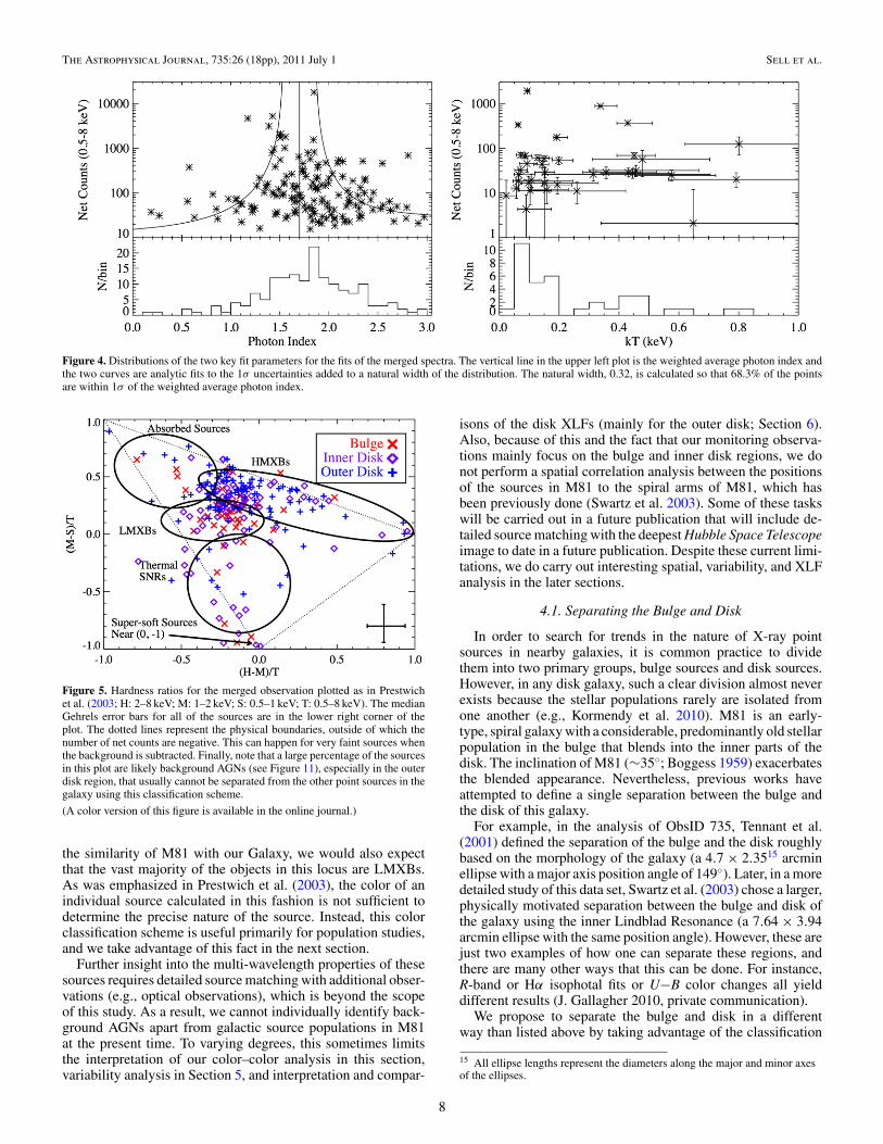
Fit parameter distributions are shown in Figure 4. Thereappears to be no correlation between the net counts and theblackbody temperature for the softest sources, although thereis a lower cutoff in the blackbody temperature, which is likelydue to the dropoff in sensitivity of Chandra at lower energiesand foreground absorption. The distribution of photon indicescan almost entirely be accounted for by the uncertainties in thephoton indices (∼68.3% within 1σ of the mean) with a naturalwidth of 0.32 to the distribution.

For each source in the master and borderline source lists,we compile one table for our merged source photometry andanother for our merged spectral fits (Tables 3 and 4).

4. HARDNESS RATIOS

Following Prestwich et al. (2003), we calculate hardnessratios using the AE pipeline for the sources in our master sourcelist (Figure 5) from the background-subtracted counts of themerged observation in different bands (H: 2–8 keV; M: 1–2 keV;S: 0.5–1 keV; T: 0.5–8 keV). Since most of the sources have fartoo few counts to make significant statements about the sourceproperties, we use these hardness ratios to estimate the spectralproperties of the differing source populations in this data set.The population of sources shows the full range of expectedcolors as seen in Figure 5.

This classification is based on the general characteristicsof the HMXB and LMXB populations in our Galaxy. Theformer are predominantly pulsar X-ray binaries and hence havehard spectra, while the latter host either black holes or low-magnetic field neutron stars resulting in softer spectra (at leastat the luminosities that we are probing with these observations).HMXBs with black holes could also be in the same locus but,in our Galaxy, these are substantially rarer than LMXBs. Given

7


Figure 4. Distributions of the two key fit parameters for the fits of the merged spectra. The vertical line in the upper left plot is the weighted average photon index andthe two curves are analytic fits to the 1σ uncertainties added to a natural width of the distribution. The natural width, 0.32, is calculated so that 68.3% of the pointsare within 1σ of the weighted average photon index.

Figure 5. Hardness ratios for the merged observation plotted as in Prestwichet al. (2003; H: 2–8 keV; M: 1–2 keV; S: 0.5–1 keV; T: 0.5–8 keV). The medianGehrels error bars for all of the sources are in the lower right corner of theplot. The dotted lines represent the physical boundaries, outside of which thenumber of net counts are negative. This can happen for very faint sources whenthe background is subtracted. Finally, note that a large percentage of the sourcesin this plot are likely background AGNs (see Figure 11), especially in the outerdisk region, that usually cannot be separated from the other point sources in thegalaxy using this classification scheme.


the similarity of M81 with our Galaxy, we would also expectthat the vast majority of the objects in this locus are LMXBs.As was emphasized in Prestwich et al. (2003), the color of anindividual source calculated in this fashion is not sufficient todetermine the precise nature of the source. Instead, this colorclassification scheme is useful primarily for population studies,and we take advantage of this fact in the next section.

Further insight into the multi-wavelength properties of thesesources requires detailed source matching with additional obser-vations (e.g., optical observations), which is beyond the scopeof this study. As a result, we cannot individually identify back-ground AGNs apart from galactic source populations in M81at the present time. To varying degrees, this sometimes limitsthe interpretation of our color–color analysis in this section,variability analysis in Section 5, and interpretation and compar-

isons of the disk XLFs (mainly for the outer disk; Section 6).Also, because of this and the fact that our monitoring observa-tions mainly focus on the bulge and inner disk regions, we donot perform a spatial correlation analysis between the positionsof the sources in M81 to the spiral arms of M81, which hasbeen previously done (Swartz et al. 2003). Some of these taskswill be carried out in a future publication that will include de-tailed source matching with the deepest Hubble Space Telescopeimage to date in a future publication. Despite these current limi-tations, we do carry out interesting spatial, variability, and XLFanalysis in the later sections.

4.1. Separating the Bulge and Disk

In order to search for trends in the nature of X-ray pointsources in nearby galaxies, it is common practice to dividethem into two primary groups, bulge sources and disk sources.However, in any disk galaxy, such a clear division almost neverexists because the stellar populations rarely are isolated fromone another (e.g., Kormendy et al. 2010). M81 is an early-type, spiral galaxy with a considerable, predominantly old stellarpopulation in the bulge that blends into the inner parts of thedisk. The inclination of M81 (∼35◦; Boggess 1959) exacerbatesthe blended appearance. Nevertheless, previous works haveattempted to define a single separation between the bulge andthe disk of this galaxy.

For example, in the analysis of ObsID 735, Tennant et al.(2001) defined the separation of the bulge and the disk roughlybased on the morphology of the galaxy (a 4.7 × 2.3515 arcminellipse with a major axis position angle of 149◦). Later, in a moredetailed study of this data set, Swartz et al. (2003) chose a larger,physically motivated separation between the bulge and disk ofthe galaxy using the inner Lindblad Resonance (a 7.64 × 3.94arcmin ellipse with the same position angle). However, these arejust two examples of how one can separate these regions, andthere are many other ways that this can be done. For instance,R-band or Hα isophotal fits or U−B color changes all yielddifferent results (J. Gallagher 2010, private communication).

We propose to separate the bulge and disk in a differentway than listed above by taking advantage of the classification

15 All ellipse lengths represent the diameters along the major and minor axesof the ellipses.

8


scheme laid out by Prestwich et al. (2003). We can use thisdiagram as a guide to separate the bulge and disk of this galaxysince certain populations of sources tend to be more stronglyassociated with different parts of the galaxy. For example,although we expect to find LMXBs in all regions of the galaxy,we expect a large fraction of the sources in the bulge region tobe LMXBs since older stellar populations dominate here. Also,we expect to see very few or no HMXBs or SNRs in the bulgeregion since these sources should only be found in regions ofactive star formation, primarily the disk.

By taking different inclination-corrected radial cuts, we canfind at which radius sources with colors consistent with LMXBsand HMXBs dominate or when they are hardly present at all.Following this technique, we define the “bulge” to include allsources inside a 4 × 2 arcmin ellipse at a position angle of 149◦with respect to the major axis, which is slightly smaller than themorphology-based definition in Tennant et al. (2001). We definethe “outer disk” to be all sources outside a 11×5.5 arcmin ellipsewith the same position angle, but within the hatched regions ofFigure 1 (∼41 arcmin2), which is closer to but considerablylarger than the disk as defined in Swartz et al. (2003), based onthe inner Lindblad Resonsance.

This method leaves an undetermined inclination-correctedannular region of the galaxy, which we refer to as the “innerdisk” region. This region includes sources from all sectionsof the color–color plot and is consistent with the properties ofboth the bulge and the disk of the galaxy. The apparent prop-erties of the incompleteness-corrected XLFs are also consis-tent with the properties of both the bulge and the disk of thegalaxy, although the fits suggest that the XLF is very disk-like(Section 6).

5. INDIVIDUAL SOURCE VARIABILITY

5.1. Flux Variability

Since one of the primary goals of this study is to test thesignificance of source variability on the XLFs, we need tofirst estimate the level of variability that we can detect in theindividual source population. We parameterize individual sourcevariability by comparing the difference in luminosity for eachsource in each observation with its corresponding uncertainties.Since we probe different timescales, we parameterize thevariability in two ways.

First, for each source, we calculate the significance statisticbetween each of the individual ObsIDs 5935–5949, whichprobes the days–weeks timescales. We use the same variabilityparameterization as in Fridriksson et al. (2008):

Sflux = maxi,j

|Fi − Fj |√σ 2

Fi+ σ 2

Fj

, (1)

where the fluxes (Fi, Fj ) were calculated as described inSection 3.3. We estimate the uncertainty in the flux (σFi

, σFj)

from the 90% confidence interval in the counts (Kraft et al.1991), and then take the average of the uneven Poisson uncer-tainties to form a single uncertainty as required by Equation (1).Second, we calculate the significance statistic on the 5 yeartimescale by comparing the weighted average fluxes and appro-priately propagated uncertainties of the merged observation tothe fluxes in ObsID 735 using Equation (1).

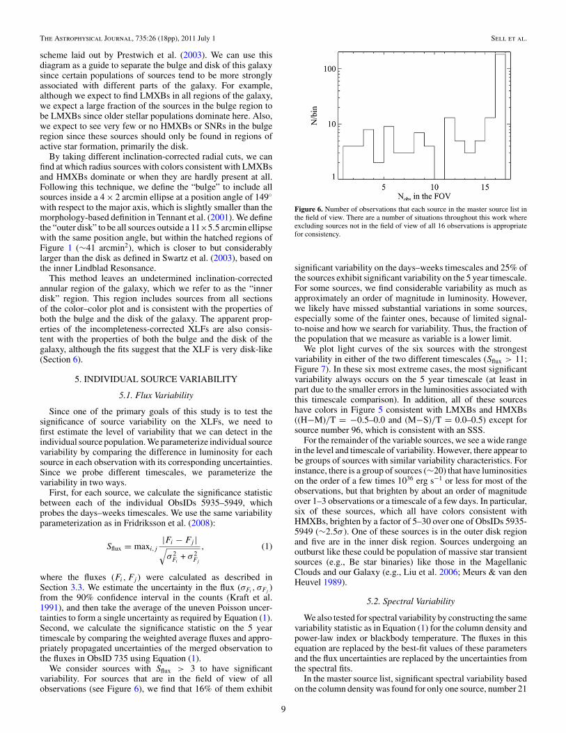
We consider sources with Sflux > 3 to have significantvariability. For sources that are in the field of view of allobservations (see Figure 6), we find that 16% of them exhibit

Figure 6. Number of observations that each source in the master source list inthe field of view. There are a number of situations throughout this work whereexcluding sources not in the field of view of all 16 observations is appropriatefor consistency.

significant variability on the days–weeks timescales and 25% ofthe sources exhibit significant variability on the 5 year timescale.For some sources, we find considerable variability as much asapproximately an order of magnitude in luminosity. However,we likely have missed substantial variations in some sources,especially some of the fainter ones, because of limited signal-to-noise and how we search for variability. Thus, the fraction ofthe population that we measure as variable is a lower limit.

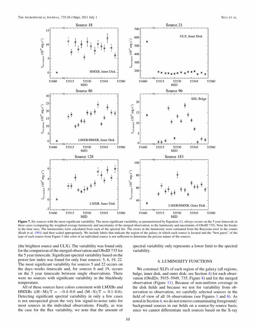
We plot light curves of the six sources with the strongestvariability in either of the two different timescales (Sflux > 11;Figure 7). In these six most extreme cases, the most significantvariability always occurs on the 5 year timescale (at least inpart due to the smaller errors in the luminosities associated withthis timescale comparison). In addition, all of these sourceshave colors in Figure 5 consistent with LMXBs and HMXBs((H−M)/T = −0.5–0.0 and (M−S)/T = 0.0–0.5) except forsource number 96, which is consistent with an SSS.

For the remainder of the variable sources, we see a wide rangein the level and timescale of variability. However, there appear tobe groups of sources with similar variability characteristics. Forinstance, there is a group of sources (∼20) that have luminositieson the order of a few times 1036 erg s−1 or less for most of theobservations, but that brighten by about an order of magnitudeover 1–3 observations or a timescale of a few days. In particular,six of these sources, which all have colors consistent withHMXBs, brighten by a factor of 5–30 over one of ObsIDs 5935-5949 (∼2.5σ ). One of these sources is in the outer disk regionand five are in the inner disk region. Sources undergoing anoutburst like these could be population of massive star transientsources (e.g., Be star binaries) like those in the MagellanicClouds and our Galaxy (e.g., Liu et al. 2006; Meurs & van denHeuvel 1989).

5.2. Spectral Variability

We also tested for spectral variability by constructing the samevariability statistic as in Equation (1) for the column density andpower-law index or blackbody temperature. The fluxes in thisequation are replaced by the best-fit values of these parametersand the flux uncertainties are replaced by the uncertainties fromthe spectral fits.

In the master source list, significant spectral variability basedon the column density was found for only one source, number 21

9


Figure 7. Six sources with the most-significant variability. The most-significant variability, as parameterized by Equation (1), always occurs on the 5 year timescale inthese cases (comparing the weighted average luminosity and uncertainty of the merged observation, to the luminosity and uncertainty of ObsID 735). Note the breaksin the time axes. The luminosities were calculated from each of the spectral fits. The errors in the luminosity were estimated from the Bayesian error in the counts(Kraft et al. 1991) and then scaled appropriately. We include labels that indicate the region of the galaxy in which each source is located and the “best guess” of thetype of each source from Figure 5 (the color of an individual source is not sufficient to determine the precise nature of the source).

(the brightest source and ULX). The variability was found onlyfor the comparison of the merged observation and ObsID 735 forthe 5 year timescale. Significant spectral variability based on thepower-law index was found for only four sources: 5, 6, 19, 22.The most significant variability for sources 5 and 22 occurs onthe days–weeks timescale and, for sources 6 and 19, occurson the 5 year timescale between single observations. Therewere no sources with significant variability in the blackbodytemperature.

All of these sources have colors consistent with LMXBs andHMXBs ((H−M)/T = −0.4–0.0 and (M−S)/T = 0.1–0.6).Detecting significant spectral variability in only a few casesis not unexpected given the very low signal-to-noise ratio formost sources in the individual observations. Finally, as wasthe case for the flux variability, we note that the amount of

spectral variability only represents a lower limit to the spectralvariability.

6. LUMINOSITY FUNCTIONS

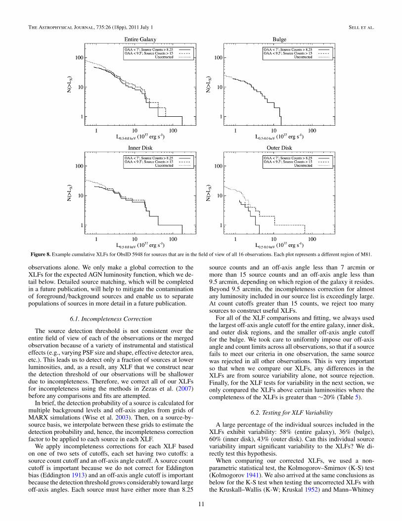
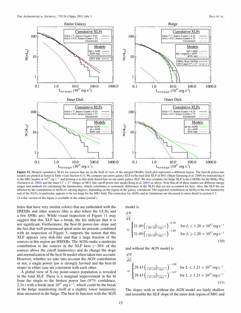
We construct XLFs of each region of the galaxy (all regions,bulge, inner disk, and outer disk; see Section 4) for each obser-vation (ObsIDs: 5935–5949, 735; Figure 8) and for the mergedobservation (Figure 11). Because of non-uniform coverage inthe disk fields and because we test for variability from ob-servation to observation, we carefully selected sources in thefield of view of all 16 observations (see Figures 1 and 6). Asnoted in Section 4, we do not remove contaminating foreground/background sources in our fields on a source-by-source basis,since we cannot differentiate such sources based on the X-ray

10


Figure 8. Example cumulative XLFs for ObsID 5948 for sources that are in the field of view of all 16 observations. Each plot represents a different region of M81.

observations alone. We only make a global correction to theXLFs for the expected AGN luminosity function, which we de-tail below. Detailed source matching, which will be completedin a future publication, will help to mitigate the contaminationof foreground/background sources and enable us to separatepopulations of sources in more detail in a future publication.

6.1. Incompleteness Correction

The source detection threshold is not consistent over theentire field of view of each of the observations or the mergedobservation because of a variety of instrumental and statisticaleffects (e.g., varying PSF size and shape, effective detector area,etc.). This leads us to detect only a fraction of sources at lowerluminosities, and, as a result, any XLF that we construct nearthe detection threshold of our observations will be shallowerdue to incompleteness. Therefore, we correct all of our XLFsfor incompleteness using the methods in Zezas et al. (2007)before any comparisons and fits are attempted.

In brief, the detection probability of a source is calculated formultiple background levels and off-axis angles from grids ofMARX simulations (Wise et al. 2003). Then, on a source-by-source basis, we interpolate between these grids to estimate thedetection probability and, hence, the incompleteness correctionfactor to be applied to each source in each XLF.

We apply incompleteness corrections for each XLF basedon one of two sets of cutoffs, each set having two cutoffs: asource count cutoff and an off-axis angle cutoff. A source countcutoff is important because we do not correct for Eddingtonbias (Eddington 1913) and an off-axis angle cutoff is importantbecause the detection threshold grows considerably toward largeoff-axis angles. Each source must have either more than 8.25

source counts and an off-axis angle less than 7 arcmin ormore than 15 source counts and an off-axis angle less than9.5 arcmin, depending on which region of the galaxy it resides.Beyond 9.5 arcmin, the incompleteness correction for almostany luminosity included in our source list is exceedingly large.At count cutoffs greater than 15 counts, we reject too manysources to construct useful XLFs.

For all of the XLF comparisons and fitting, we always usedthe largest off-axis angle cutoff for the entire galaxy, inner disk,and outer disk regions, and the smaller off-axis angle cutofffor the bulge. We took care to uniformly impose our off-axisangle and count limits across all observations, so that if a sourcefails to meet our criteria in one observation, the same sourcewas rejected in all other observations. This is very importantso that when we compare our XLFs, any differences in theXLFs are from source variability alone, not source rejection.Finally, for the XLF tests for variability in the next section, weonly compared the XLFs above certain luminosities where thecompleteness of the XLFs is greater than ∼20% (Table 5).

6.2. Testing for XLF Variability

A large percentage of the individual sources included in theXLFs exhibit variability: 58% (entire galaxy), 36% (bulge),60% (inner disk), 43% (outer disk). Can this individual sourcevariability impart significant variability to the XLFs? We di-rectly test this hypothesis.

When comparing our corrected XLFs, we used a non-parametric statistical test, the Kolmogorov–Smirnov (K-S) test(Kolmogorov 1941). We also arrived at the same conclusions asbelow for the K-S test when testing the uncorrected XLFs withthe Kruskall–Wallis (K-W; Kruskal 1952) and Mann–Whitney

11


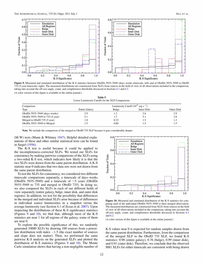
Figure 9. Measured and simulated distribution of the K-S statistics between ObsIDs 5935–5949 (days–weeks timescale; left) and of ObsIDs 5935–5949 to ObsID735 (5 year timescale; right). The measured distributions are constructed from XLFs from sources in the field of view of all observations included in the comparison,taking into account the off-axis angle, count, and completeness thresholds discussed in Sections 6.1 and 6.2.


Table 5Lower Luminosity Cutoffs for the XLF Comparisons

Comparison Luminosity Cutoff (1037 erg s−1)Type Entire Galaxy Bulge Inner Disk Outer Disk

ObsIDs 5935–5949 (days–weeks) 2.9 1.3 2.6 2.9ObsIDs 5935–5949 to 735 (5 year) 5.1 1.7 5.1 3.8Merged to ObsID 735 (5 year) 1.8 0.33 1.5 1.3ObsIDs 5935–5949 to Merged 1.5 0.80 1.5 1.5

Note. We include the comparison of the merged to ObsID 735 XLF because it goes considerably deeper.

(M-W) tests (Mann & Whitney 1947). Helpful detailed expla-nations of these and other similar statistical tests can be foundin Siegel (1956).

The K-S test is useful because it could be applied tothe incompleteness-corrected XLFs. We tested our XLFs forconsistency by making pairwise comparisons of the XLFs usinga two-sided K-S test, which indicates how likely it is that thetwo XLFs were drawn from the same parent distribution. A K-Sstatistic near 0 indicates that two data sets were not drawn fromthe same parent distribution.

To test the XLFs for consistency, we considered two differenttimescale comparisons separately, a timescale of days–weeks(ObsIDs 5935–5949) and a timescale of ∼5 years (ObsIDs5935–5949 to 735 and merged to ObsID 735). In doing so,we also compared the XLFs in each of our different fields ofview separately (entire galaxy, bulge, inner disk, and outer diskregions). In addition, we test for the possibility that differencesin the merged and individual XLFs arise because of differencesin individual source luminosities in a snapshot versus theaverage luminosity (see Section 4.1 of Zezas et al. 2007). Uponinspecting the distributions of these K-S significance statistics(Figures 9 and 10), we find that, although most of the K-Sstatistics are near 1 for all regions of the galaxy, some of themare near 0.

To explore the possible significance of this, we randomlygenerated 10000 XLFs by drawing 100 sources from a power-law distribution with index −1.5 (the exact number of sourcesand slope does not matter). Then, we performed the samepairwise K-S analysis on the generated XLFs and plotted thedistribution of K-S statistics (Figures 9 and 10). The MonteCarlo simulation shows that having a non-negligible number of

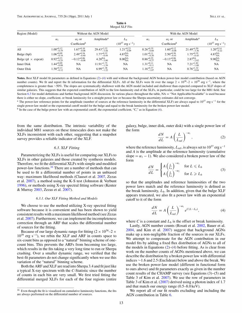
Figure 10. Measured and simulated distribution of the K-S statistics for com-paring each of the individual ObsIDs 5935–5949 to their merged observation.The measured distributions are constructed from XLFs from sources in the fieldof view of all observations included in the comparison, taking into account theoff-axis angle, count, and completeness thresholds discussed in Sections 6.1and 6.2.


K-S values near 0 is expected for random samples drawn fromthe same parent distribution. Furthermore, from the comparisonof the merged XLF to the ObsID 735 XLF, we found K-Sstatistics: 0.98 (entire galaxy), 0.76 (bulge), 0.99 (inner disk),and 0.91 (outer disk). Therefore, we conclude that the observedM81 XLFs for either timescale are consistent with being drawn

12


Table 6Merged XLF Fits

Region (Model) Without the AGN Model With the AGN Model

α1 α2 or Amplitudea Lb α1 α2 or Amplitudea Lb

Coefficientb (1037 erg s−1) Coefficientb (1037 erg s−1)

All 1.00+0.12−0.19 1.67+0.10

−0.08 29.43+3.32−3.44 1.21+0.23

−0.09 0.26+0.35−0.60 1.60+0.12

−0.08 21.49+4.50−3.36 1.20+0.14

−0.22

Bulge (bpl) 1.06+0.09−0.18 2.49+0.54

−0.40 1.77+0.32−0.44 4.87NA

NA 1.01+0.11−0.20 2.50+0.56

−0.41 1.75+0.35−0.45 4.87NA

NA

Bulge (pl × expcut) 0.92+0.23−0.25 −0.12+0.06

−0.08 4.20NA−3.80 8.00NA

NA 0.86+0.25−0.27 −0.13+0.06

−0.08 2.87NA−2.82 9.90NA

NA

Inner Disk 1.44+0.09−0.08 NA 11.91+1.75

−1.59 NA 1.31+0.11−0.11 NA 7.21+1.82

−1.68 NA

Outer Disk 1.58+0.13−0.12 NA 6.99+1.38

−1.22 NA 1.16+0.37−1.07 NA 0.76+1.32

−0.84 NA

Notes. Best XLF model fit parameters as defined in Equations (2)–(4) with and without the background AGN broken power-law model contribution (based on AGNnumber counts). We fit and report the fit information for the differential XLFs. All of the XLFs were fit over the range 2 × 1036–2 × 1039 erg s−1, where thecompleteness is greater than ∼50%. The slopes are systematically shallower with the AGN model included and shallower than expected compared to XLF slopes ofsimilar galaxies. This suggests that the expected contribution of AGN to the low-luminosity end of the XLFs, in particular, could be too large for the M81 field. SeeSection 6.3 for model definitions and further background AGN discussion. In various places throughout the table, NA = “Not Applicable/Available” is used becausethere is either no slope, coefficient, or break luminosity for a straight power law or because the Sherpa uncertainty estimates did not converge.a The power-law reference points for the amplitude (number of sources at the reference luminosity in the differential XLF) are always equal to 1037 erg s−1 for thesingle power-law model or the exponential cutoff model for the bulge and equal to the break luminosity for the broken power-law model.b In the case of the bulge power law with an exponential cutoff, the exponential coefficient, “C,” as in Equation (4).

from the same distribution. The intrinsic variability of theindividual M81 sources on these timescales does not make theXLFs inconsistent with each other, suggesting that a snapshotsurvey provides a reliable indicator of the XLF.

6.3. XLF Fitting

Parameterizing the XLFs is useful for comparing our XLFs toXLFs in other galaxies and those created by synthesis models.Therefore, we fit the differential XLFs with simple and modifiedpower-law functions.16 There are a number of methods that canbe used to fit a differential number of points in an unbiasedway: maximum likelihood methods (Clauset et al. 2007, Zezaset al. 2007), a method using the K-S test (Johnston & Verbunt1996), or methods using X-ray spectral fitting software (Kenter& Murray 2003, Zezas et al. 2007).

6.3.1. Our XLF Fitting Method and Models

We choose to use the method utilizing X-ray spectral fittingsoftware because it is convenient and has been shown to yieldconsistent results with a maximum likelihood method (see Zezaset al. 2007). Furthermore, we can implement the incompletenesscorrection through an ARF that scales the differential numberof sources for the fitting.

Because of our large dynamic range for fitting (2 × 1036–2 ×1039 erg s−1), we rebin the XLF and ARF in counts space tosix-count bins as opposed to a “natural” binning scheme of one-count bins. This prevents the ARFs from becoming too large,which results in the fits taking a very long time to run or Sherpacrashing. Over a smaller dynamic range, we verified that thebest-fit parameters do not change significantly when we use thisvariation of the “natural” binning scheme.

Both the ARF and XLF are read into Sherpa 3.4 and fit just likea typical X-ray spectrum with the C-Statistic since the numberof counts in each bin are very small. We first tried fitting thedifferential merged XLFs for each of the four regions (entire

16 Even though the fit is visualized on cumulative luminosity functions, the fitsare always performed on the differential number of sources.

galaxy, bulge, inner disk, outer disk) with a single power law ofthe form

dN

dL= A

(L

Lref

)−α1

, (2)

where the reference luminosity, Lref , is always set to 1037 erg s−1

and A is the amplitude at the reference luminosity (cumulativeslope = α1 − 1). We also considered a broken power law of theform

dN

dL=

⎧⎨⎩

A(

LLb

)−α1

for L � Lb

A(

LLb

)−α2

for L � Lb

(3)

so that the amplitudes and reference luminosities of the twopower laws match and the reference luminosity is defined asthe break luminosity, Lb. In addition, given that the bulge XLFappears truncated, we also fit a power law with an exponentialcutoff to it of the form

dN

dL= A

(L

Lref

)−α1

eC(L−Lb), (4)

where C is a constant and Lb is the offset or break luminosity.Lastly, AGN number counts (Rosati et al. 2002, Bauer et al.

2004, and Kim et al. 2007) suggest that background AGNsmake up a non-negligible fraction of the sources in our XLFs.We attempt to compensate for the AGN contribution in ourmodel fits by adding a fixed flux distribution of AGNs to all ofthe models in Equations (2)–(4) before fitting. As is clear fromwork on the number counts of AGNs mentioned above, we candescribe the distribution by a broken power law with differentialindices ∼1.6 and 2.5 (Euclidean) below and above the break. Weuse the broken power-law model (different in functional formto ours above) and fit parameters exactly as given in the numbercount results of the CHAMP survey (see Equations (3)–(5) andTable 3 of Kim et al. 2007). We use the row of parameters inTable 3 of Kim et al. (2007) derived using a photon index of 1.7and that match our energy range (0.5–8.0 keV).

We report all of our fit results excluding and including theAGN contribution in Table 6.

13


6.3.2. Discussion of XLF Fit Results by Region

First, the contribution from AGNs is a serious issue in mostof our fields. The AGN contribution increases at smaller fluxesbecause it appears that the log N–log S slope is steeper thanthe slope of the M81 XLF. At face value, including the AGNdistribution forces the best-fit power-law slopes for M81 to beshallower in all of the XLFs. However, foreground absorption ofM81 brings about an uncertainty in the AGN flux distribution.The foreground absorption is difficult to quantify because theclumpiness of the disk suggests a highly variable columndensity. A disk scale height of a few hundred parsecs for atypical interstellar medium density of ∼1 cm−3 at the inclinationof M81 (∼35◦; Boggess 1959) produces an average columndensity ∼1021 cm−2 measured perpendicular to the disk. Thiscould decrease the flux of a typical AGN by ∼10%, flatteningthe faint-end slope of log N–log S for AGNs in this region.

The uncertainty from foreground absorption together withgalactic foreground diffuse emission from M81, standard errorsin the survey measurements, and cosmic variance make inter-preting our XLFs very difficult, especially at the faint ends. Forexample, an uncertainty of ∼20% due to cosmic variance andan equally sizable shift brought about by the foreground emis-sion and absorption of M81 changes the best-fit slope of theouter disk by ∼0.1 and the amplitude by ∼70%. Note that theAGN contamination varies with the galactic source density (seeTable 6 and Figure 11) so that the bulge XLF is least affectedand the outer disk XLF is most affected. In light of these com-plications, we are still able to make some concrete statementsregarding our XLFs.

In order to interpret our XLF fits, we need to comparethe significance of the fits between the single and brokenpower-law models. Since the C-Statistic, a maximum likelihoodstatistic, is used, it is appropriate to compare the quality ofthe fits using a likelihood ratio test (e.g., Zezas et al. 2007).We simulate 1000 XLFs from a single power-law model andthen fit them with the single and the broken power-law modelin the same way that we fit the observed XLFs. We thencalculate the ratio of the single to the broken power-law best-fitC-statistics for each XLF. The confidence level correspondingto the amount of improvement of the fit from the single tothe broken power-law model is the fraction of times thatthe simulated ratio of statistics is greater than the measuredratio of the statistics. One should not judge the quality of thefits from the best-fit cumulative distribution functions on thelogarithmically scaled plots because they can be misleading.For instance, uncertainties in the XLFs at the high-luminosityend are much larger than those at the low-lumionsity end. Inaddition, unexpected statistical effects frequently caused by theskewness in the probability distribution of sources comprisingthe XLFs have been documented previously (Gilfanov et al.2004; Clauset et al. 2007).

In the bulge, we find that the broken power-law modeland the power-law model with an exponential cutoff providea highly significant improvement in the fit versus a singlepower law (>99.9% confidence, �3σ ). The break luminosityis poorly constrained but is within a factor of a few of theEddington luminosity of a neutron star and is consistent withthe values derived from other previous work for elliptical andS0 galaxies, the bulges of other galaxies, and the LMXBs ofour Galaxy (Sarazin et al. 2000; Blanton et al. 2001; Kunduet al. 2002; Grimm et al. 2002; Kim et al. 2006; Voss et al.2009). We also see evidence of the flattening of the LMXBXLF below ∼1037 erg s−1 that has been seen by many of

these previous studies. The best-fit functions with the AGNmodel are

dN

dL

⎧⎪⎨⎪⎩

1.75(

L4.87×1037 erg s−1

)−1.01for L � 4.87 × 1037 erg s−1

1.75(

L4.87×1037 erg s−1

)−2.50for L � 4.87 × 1037 erg s−1

(5)for the broken power law and

dN

dL= 2.87

(L

1037 erg s−1

)−0.86

e−0.13(L−9.9×1037 erg s−1) (6)

for the power law with an exponential cutoff.The shape of this XLF together with the locations of the

sources in the color–color plot (Figure 5) suggests a veryold population of stars dominates the innermost part of M81and that we are probing a population of mostly LMXBs.The shape of the XLF is also consistent with the overallshape of the average LMXB XLF, which has a flat cumulativedistribution below a few times 1037 erg s−1 with a cutoff neara few times 1038 erg s−1 (Gilfanov 2004). The AGNs do notstrongly bias these results as they are expected to comprise�10% of the sources in the XLF above the cutoff luminosity,2 × 1036 erg s−1.

Next, because of the very large percentage of AGNs expectedin the outer disk XLF (∼80% of the sources above the cutoffluminosity and ∼60% of the sources above 1037 erg s−1), thisregion is the most difficult to interpret. This region also has thefewest total number of sources, and brief inspection of some all-sky optical surveys suggests that there are also a few foregroundstars, which we have not attempted to remove. While thereappears to be a break near 1037 erg s−1, it does not bring abouta significant improvement in the fit when the AGN contributionis taken into account (94% confidence, 1.9σ ).

Therefore, we fit this XLF with a single, unbroken power lawas is typically seen in disk-like regions of ongoing star formationas in the disk XLF of our Galaxy (Grimm et al. 2002), theAntennae (Zezas et al. 2007), and NGC 6946 (Fridriksson et al.2008), for examples. The best-fit function with the AGN modelis

dN

dL= 0.76

(L

1037 erg s−1

)−1.16

(7)

with a much shallower slope than what has been found inthe studies above and which produces an unusual-looking fit(Figure 11). However, the best-fit function without the AGNmodel is

dN

dL= 6.99

(L

1037 erg s−1

)−1.58

(8)

with a slope that is more consistent with the other disk studiesabove. The slope cannot be well constrained and, given the largefit uncertainties (the errors for the slopes are on the order of therange of slopes found with or without the AGN model), we donot attempt to interpret this XLF further.

Our inner disk region XLF is consistent with a single,unbroken power law and a broken power law does not resultin a significant improvement in the fit (44% confidence, <1σ ).The best-fit function with the AGN model is

dN

dL= 7.21

(L

1037 erg s−1

)−1.31

. (9)

Inspection of the color–color plot (Figure 5) indicates that thereare a population of LMXBs in this region (or HMXBs with black

14


Figure 11. Merged cumulative XLFs for sources that are in the field of view of the merged ObsIDs. Each plot represents a different region. The best-fit power-lawmodels are plotted as listed in Table 4 (see Section 6.3). We compare our entire galaxy XLF to the total disk XLF of M31 (Shaw Greening et al. 2009) by normalizing itto the M81 models at 1037 erg s−1 and plotting it as dim dash-dotted line on our entire galaxy XLF. We also compare our bulge XLF to the LMXBs for the Milky Way(Grimm et al. 2002) and the inner 17′ × 17′ (bulge) of M31 (the cutoff power-law model Kong et al. 2003) as above. Note that all of these studies use different energyranges and methods for calculating the luminosities, which contributes to systematic differences in the XLFs that are not accounted for here. Also, the XLF fits areaffected by the contribution of AGNs to varying degrees, depending on the region of the galaxy considered. The expected contribution of AGNs to the low-luminosityend of the XLFs, in particular, appears to be too large for the M81 field. The correction for AGNs and its limitations are discussed in more detail in section 6.3.


holes that have very similar colors) that are embedded with theHMXBs and other sources (this is also where the ULXs anda few SNRs are). While visual inspection of Figure 11 maysuggest that this XLF has a break, the fits indicate that it isnot significant. Furthermore, the best-fit power-law slope andthe fact that well-pronounced spiral arms are present, combinedwith an inspection of Figure 5, supports the notion that thisXLF appears very disk-like and that a large fraction of thesources in this region are HMXBs. The AGNs make a moderatecontribution to the sources in the XLF here (∼30% of thesources above the cutoff luminosity) and do change the slopeand normalization of the best-fit model when taken into account.However, whether we take into account the AGN contributionor not, a single power law is strongly favored and the best-fitslopes in either case are consistent with each other.

A global view of X-ray point-source population is revealedin the total XLF. There is a marginal improvement in the fitfrom the single to the broken power law (97% confidence,2.2σ ) with a break near 1037 erg s−1, which could be the breakin the bulge manifesting itself at a slightly lower luminositythan measured in the bulge. The best-fit function with the AGN

model is

dN

dL

=

⎧⎪⎨⎪⎩

21.49(

L1.20×1037 erg s−1

)−0.26for L � 1.20 × 1037 erg s−1

21.49(

L1.20×1037 erg s−1

)−1.60for L � 1.20 × 1037 erg s−1

(10)

and without the AGN model is

dN

dL

=

⎧⎪⎨⎪⎩

29.43(

L1.21×1037 erg s−1

)−1.00for L � 1.21 × 1037 erg s−1

29.43(

L1.21×1037 erg s−1

)−1.67for L � 1.21 × 1037 erg s−1

.

(11)

The slopes with or without the AGN model are fairly shallowand resemble the XLF slope of the inner disk region of M81 and

15


disk regions in other galaxies where there is considerable starformation occurring. However, because this XLF does also havea significant break and the color–color plot (Figure 5) suggestscontributions from many different populations of sources, weconclude that this XLF is neither disk- nor bulge-dominated,but is a fairly even mixture of both types.

Finally, we can use our XLFs to estimate two interestinggalactic properties: the stellar mass and the SFR, using relation-ships in Gilfanov (2004) and Grimm et al. (2003), respectively.

First, to estimate the total stellar mass of M81, we need toestimate the number of LMXBs in M81 with LX > 1037 erg s−1.Since we have found that the bulge is likely almost exclusivelycomposed of LMXBs, we use our bulge XLF to estimate thatthere are ∼20 LMXBs in this range. As we have stated above,we also expect there to be a population of LMXBs in the diskregions as well, especially in the inner disk region. The fractionof LMXBs can be estimated from our color–color plot (Figure 5)but is very uncertain. Taking this fraction and applying it toour XLF in this luminosity range, we estimate that there are∼10 LMXBs in this region. The outer disk region appears tocontribute only a very small amount of LMXBs with LX >1037 erg s−1 when the expected AGN fraction is taken intoaccount, so we do not include it here.

Then using these numbers together with Equation (20) inGilfanov (2004), we estimate that the total stellar mass of M81is > 2.1 × 1010 M�. This is a fairly robust lower limit to thenumber LMXBs in M81 because we have neglected the outerdisk contribution, the K-band light is measured out to largerradii than our X-ray data, there are some sources superimposedagainst the LINER nucleus that we are unable to detect orclassify (some of these are the ML sources in Table 2), andEquation (21) suggests a larger mass.

We also estimate the total stellar mass of M81 using the total2MASS K-band magnitude, ∼3.9 mag. This corresponds to asolar K-band luminosity of 7.7 × 1010 L�. Using M∗/LK ≈ 1.1from GALEV models for an SAab-type galaxy (Kotulla et al.2009), we estimate a total stellar mass of 8.5 × 1010 M�.Reversing the calculation, this stellar mass suggests that M81has ∼70–120 LMXBs with LX > 1037 erg s−1. Part of thisdiscrepancy can be attributed to the reasons listed at the end ofthe previous paragraph. Other reasons include uncertainties inthe M∗/LK ratio of M81 and of the values assumed by Gilfanov(2004), which, together, could contribute deviations of factorsof approximately two to three. For these reasons, caution shouldbe taken in estimating the number of LMXBs and stellar massusing this method for M81 and other galaxies with similarissues.

Second, to estimate the SFR, we need to estimate the totalnumber of HMXBs and their total luminosity for L2–10 keV >2 × 1038 erg s−1. There are four sources with L2–10 keV > 2 ×1038 erg s−1. Inspection of the locations of these sourcesin Figure 5 suggests that at least one of these sources islikely to be an HMXB. The other three sources all lie onthe boundary between HMXBs and LMXBs. This, combinedwith the knowledge that the color of an individual source isnot sufficient to determine the precise nature of the source(Section 4), and the fact that we are subject to large Poissonerrors at the high-luminosity end of the XLF, only allows usto place approximate limits on the SFR estimated with thismethod. Equation (20) of Grimm et al. (2003) suggests arange of SFRs of 0.34–1.38 M� yr−1 for 1–4 sources withL2–10 keV > 2 × 1038 erg s−1, and Equation (22) of Grimmet al. (2003) suggests a range of SFRs of 0.52–1.02 M� yr−1

for the range of luminosities of these sources, 1.34–2.64 ×1039 erg s−1. These estimates are comparable to the SFR that hasbeen estimated for M81 based on a combination of ultraviolet,Hα, and infrared observations (0.3–0.9 M� yr−1; e.g., Gordonet al. 2004).

7. COMPARING THE XLFs OF M81 WITH THOSE OFTWO OTHER NEARBY SIMILAR SPIRAL GALAXIES

M81, M31, and our Milky Way are all Sb-type galaxies withsimilar SFRs near 1 M� yr−1. Below, we make comparisonsof the global properties of their X-ray binary populations usingtheir XLFs.

7.1. Comparisons with the Milky Way

First, the XLFs of both the inner and outer disk regions of M81are systematically shallower than the HMXB slope of the MilkyWay, but, given the statistical uncertainties and uncertainties inthe AGN contribution, are fairly consistent with one another.While the M81 inner and outer disk regions do appear to bedominated by HMXBs, they also contain other types of sources(e.g., AGN, SNRs) that we are unable to separate conclusivelyon an individual basis at the present time.

Second, the near match of the M81 bulge and the normalized17

LMXB population in the Milky Way is striking (Figure 11). Wefind that the low-luminosity LMXB slope of the Milky Way issimilar to the low-luminosity slope found for the M81 bulgewithin the uncertainties. Also, the cutoffs in the LMXB XLFsare within a factor of ∼2 of one another, supporting the notionthat the bulge of M81 is dominated by LMXBs as seen in thecolor–color plot (Figure 5).

7.2. Comparisons With M31

We find that the normalized XLF of the inner 17′ ×17′ regionof M31 as measured with Chandra by Kong et al. (2003) isquite similar to the bulge XLF of M81 (Figure 11). These dataalso match well to the bulge region observations measured withXMM-Newton (r < 15′) by Trudolyubov et al. (2002).

The disk XLFs of M31 are more difficult to compare asstudies of the M31 disk return different results (Kong et al.2003; Shaw Greening et al. 2009). Although the XLFs in eachof the disk regions are consistent with single, unbroken powerlaw, as expected, the power-law slopes measured by each groupare significantly different. We examine some of the reasons forthese differences below.

The disk XLFs of Kong et al. (2003) do not include ULXsor any sources brighter than ∼3 × 1037 erg s−1 (unlike thedisk XLFs in M81 and the HMXB XLF of the Milky Way).However, the field of view of Chandra is much smaller thanM31 and all of the Chandra fields in Kong et al. (2003) togetherstill only cover a fraction of the disk of M31. As noted in ShawGreening et al. (2009), there are much brighter sources seen intheir fields, which cover most of the M31 disk that are beingmissed in small-area surveys. Missing these brighter sourcescould truncate the high-luminosity end of Kong et al.’s (2003)disk XLFs, and could make these XLFs steeper. However, theeffect that a few bright sources have on the best-fit slope is notobvious without further detailed analysis, which is beyond thescope of this paper.

17 Given the biases in determining matching fields of view, blended andhidden sources in the bulge of M81, AGN contributions, etc., we do notcompare source densities in our regions.

16


Second (as pointed out in Shaw Greening et al. 2009, seetheir Figure 5), model bias in the spectral fitting of each of thepoint sources that comprise the XLF could affect the best-fitnormalization and slope of the XLF. For instance, Kong et al.(2003) fit all of their sources with a fixed, absorbed power law,which could be biasing their XLFs. We could also be slightlybiased by choosing a power law as our initial fitting model,but we expect this to have a smaller effect because we haveallowed for the possibility of a model that better describes softersources (blackbody). In addition, we float our photon index orblackbody temperature for all sources with more than 25 countsand always float our column densities for all sources with morethan 5 counts.

Thoroughly assessing the impact of a single versus a variableconversion factor on the XLFs directly is beyond the scopeof this paper. However, we can make some simple statisticalcomparisons for the merged luminosities of the sources in themaster source list. We compare the error that would arise fromusing a single conversion factor to calculate the luminosities(Figure 3) and the statistical error in the luminosity scaled fromthe Bayesian error in the counts. We find that the shape of bothdistributions is very similar, but that the median and the widthof the distribution of the statistical percent error is greater thanthe median (by approximately a factor of 1.5) and the width ofthe distribution of the percent error that would arise from usinga single conversion factor. Because the conversion factor errorsare typically smaller than the statistical errors in the luminosity,we suspect that the effect on the XLFs would probably be fairlysmall, but maybe non-negligible.

In light of these issues, we only compare our disk and entiregalaxy XLF results to the disk XLFs constructed by ShawGreening et al. (2009). The total disk XLF that these authorsconstruct surprisingly seems to better match the M81 XLF ofthe entire galaxy rather than the inner or outer disk XLFs. First,they claim a break in their total disk XLF, which happensto coincide with the measured break in the M81 XLF of theentire galaxy. Also, the power-law slopes are in good agreementwith the slopes that we measure for M81’s entire galaxy XLF.These results suggest that the disk of M31 has a high-luminositycomponent similar to what is seen in the inner and outer disks ofM81, but it also seems to have a more considerable populationof LMXBs there that produce at least a marginally significantbreak near 1037 erg s−1.

8. SUMMARY

We have presented an in-depth analysis of multiple aspectsof the X-ray source population of M81 from the perspectiveof the X-ray observations alone. We conducted our sourcedetection procedure carefully, producing a master source list of265 sources. We then extracted and individually fit the spectrafor each of these sources in each of the 16 observations ofM81 included in our analysis. With the spectral information, wecalculated hardness ratios and used the aid of a color–color plotto classify different populations of sources. From the populationstudy, we devised an alternate conservative method of separatingthe bulge and the disk of the galaxy. Then, we quantifiedthe variability of the individual sources and considered theirpossible effect on the luminosity function of the galaxy. We findthat, despite detecting significant variability in ∼36%–60% ofthe sources included in the XLFs, the XLF of M81 remainsstable at luminosities greater than ∼2 × 1037 erg s−1. Finally,we plotted and fit the XLFs, analyzed them with regard to their

point-source populations, and compared them to the XLFs ofM31 and the Milky Way.

We thank Jay Gallagher and Christy Tremonti for helpfulcomments. D.P. and P.S. gratefully acknowledge support fromChandra grant GO5-6092. A.Z. acknowledges support by theUE IRG grant 224878. Space Astrophysics at the Universityof Crete is supported by EU FP7-REGPOT grant 206469(ASTROSPACE).

REFERENCES

Angelini, L., Loewenstein, M., & Mushotzky, R. F. 2001, ApJ, 557, L35Bauer, F. E., Alexander, D. M., Brandt, W. N., Schneider, D. P., Treister, E.,

Hornschemeier, A. E., & Garmire, G. P. 2004, AJ, 128, 2048Belczynski, K., Kalogera, V., Rasio, F. A., Taam, R. E., Zezas, A., Bulik, T.,

Maccarone, T. J., & Ivanova, N. 2008, ApJS, 174, 223Blanton, E. L., Sarazin, C. L., & Irwin, J. A. 2001, ApJ, 552, 106Boggess, N. W. 1959, PASP, 71, 534Broos, P. S., Townsley, L. K., Feigelson, E. D., Getman, K. V., Bauer, F. E., &

Garmire, G. P. 2010, ApJ, 714, 1582Cash, W. 1979, ApJ, 228, 939Clauset, A., Rohilla Shalizi, C., & Newman, M. E. J. 2007, arXiv:0706.1062Colbert, E. J. M., Heckman, T. M., Ptak, A. F., Strickland, D. K., & Weaver, K.

A. 2004, ApJ, 602, 231Davis, J. E. 2001, ApJ, 562, 575Dickey, J. M., & Lockman, F. J. 1990, ARA&A, 28, 215Eddington, A. S. 1913, MNRAS, 73, 359Fabbiano, G. 1988, ApJ, 325, 544Fabbiano, G., & White, N. E. 2006, in Compact Stellar X-ray Sources, ed. W.

H. G. Lewin & M. van der Klis (Chicago, IL: Univ. Chicago Press), 475Fabbiano, G., et al. 2010, ApJ, 725, 1824Fragos, T., et al. 2008, ApJ, 683, 346Freedman, W. L., et al. 1994, ApJ, 427, 628Freeman, P., Doe, S., & Siemiginowska, A. 2001, Proc. SPIE., 4477, 76Freeman, P. E., Kashyap, V., Rosner, R., & Lamb, D. Q. 2002, ApJS, 138, 185Fridriksson, J. K., Homan, J., Lewin, W. H. G., Kong, A. K. H., & Pooley, D.

2008, ApJS, 177, 465Garmire, G. P., Bautz, M. W., Ford, P. G., Nousek, J. A., & Ricker, G. R., Jr.

2003, Proc. SPIE., 4851, 28Gehrels, N. 1986, ApJ, 303, 336Gilfanov, M. 2004, MNRAS, 349, 146Gilfanov, M., Grimm, H., & Sunyaev, R. 2004, MNRAS, 351, 1365Gordon, K. D., et al. 2004, ApJS, 154, 215Grimm, H., Gilfanov, M., & Sunyaev, R. 2002, A&A, 391, 923Grimm, H., Gilfanov, M., & Sunyaev, R. 2003, MNRAS, 339, 793Immler, S., & Wang, Q. D. 2001, ApJ, 554, 202Johnston, H. M., & Verbunt, F. 1996, A&A, 312, 80Kenter, A. T., & Murray, S. S. 2003, ApJ, 584, 1016Kilgard, R. E., Kaaret, P., Krauss, M. I., Prestwich, A. H., Raley, M. T., & Zezas,

A. 2002, ApJ, 573, 138Kim, D., & Fabbiano, G. 2004, ApJ, 611, 846Kim, D., & Fabbiano, G. 2010, ApJ, 721, 1523Kim, D., et al. 2004, ApJS, 150, 19Kim, D., et al. 2006, ApJ, 652, 1090Kim, M., Wilkes, B. J., Kim, D., Green, P. J., Barkhouse, W. A., Lee, M. G.,

Silverman, J. D., & Tananbaum, H. D. 2007, ApJ, 659, 29Kolmogorov, A. 1941, Ann. Math. Stat., 12, 461Kong, A. K. H., DiStefano, R., Garcia, M. R., & Greiner, J. 2003, ApJ, 585, 298Kormendy, J., Drory, N., Bender, R., & Cornell, M. E. 2010, ApJ, 723, 54Kotulla, R., Fritze, U., Weilbacher, P., & Anders, P. 2009, MNRAS, 396, 462Kraft, R. P., Burrows, D. N., & Nousek, J. A. 1991, ApJ, 374, 344Kruskal, W. H. 1952, Ann. Math. Stat., 23, 525Kundu, A., Maccarone, T. J., & Zepf, S. E. 2002, ApJ, 574, L5Liu, Q. Z., van Paradijs, J., & van den Heuvel, E. P. J. 2006, A&A, 455, 1165Maccarone, T. J., Kundu, A., & Zepf, S. E. 2003, ApJ, 586, 814Mann, H. B., & Whitney, D. R. 1947, Ann. Math. Stat., 18, 50Meurs, E. J. A., & van den Heuvel, E. P. J. 1989, A&A, 226, 88Pence, W. D., Snowden, S. L., Mukai, K., & Kuntz, K. D. 2001, ApJ, 561,

189Plucinsky, P. P., et al. 2008, ApJS, 174, 366Prestwich, A. H., Irwin, J. A., Kilgard, R. E., Krauss, M. I., Zezas, A., Primini,

F., Kaaret, P., & Boroson, B. 2003, ApJ, 595, 719Primini, F. A., Forman, W., & Jones, C. 1993, ApJ, 410, 615Rosati, P., et al. 2002, ApJ, 566, 667

17

http://dx.doi.org/10.1086/323026

http://adsabs.harvard.edu/abs/2001ApJ...557L..35A

http://adsabs.harvard.edu/abs/2001ApJ...557L..35A

http://dx.doi.org/10.1086/424859

http://adsabs.harvard.edu/abs/2004AJ....128.2048B

http://adsabs.harvard.edu/abs/2004AJ....128.2048B

http://dx.doi.org/10.1086/521026

http://adsabs.harvard.edu/abs/2008ApJS..174..223B

http://adsabs.harvard.edu/abs/2008ApJS..174..223B

http://dx.doi.org/10.1086/320461

http://adsabs.harvard.edu/abs/2001ApJ...552..106B

http://adsabs.harvard.edu/abs/2001ApJ...552..106B

http://dx.doi.org/10.1086/127446

http://adsabs.harvard.edu/abs/1959PASP...71..534B

http://adsabs.harvard.edu/abs/1959PASP...71..534B

http://dx.doi.org/10.1088/0004-637X/714/2/1582

http://adsabs.harvard.edu/abs/2010ApJ...714.1582B

http://adsabs.harvard.edu/abs/2010ApJ...714.1582B

http://dx.doi.org/10.1086/156922

http://adsabs.harvard.edu/abs/1979ApJ...228..939C


http://www.arxiv.org/abs/0706.1062

http://dx.doi.org/10.1086/380899



http://dx.doi.org/10.1086/323488

http://adsabs.harvard.edu/abs/2001ApJ...562..575D

http://adsabs.harvard.edu/abs/2001ApJ...562..575D

http://dx.doi.org/10.1146/annurev.aa.28.090190.001243

http://adsabs.harvard.edu/abs/1990ARA&A..28..215D

http://adsabs.harvard.edu/abs/1990ARA&A..28..215D

http://adsabs.harvard.edu/abs/1913MNRAS..73..359E

http://adsabs.harvard.edu/abs/1913MNRAS..73..359E

http://dx.doi.org/10.1086/166026

http://adsabs.harvard.edu/abs/1988ApJ...325..544F


http://adsabs.harvard.edu/abs/2006csxs.book..475F

http://dx.doi.org/10.1088/0004-637X/725/2/1824

http://adsabs.harvard.edu/abs/2010ApJ...725.1824F

http://adsabs.harvard.edu/abs/2010ApJ...725.1824F

http://dx.doi.org/10.1086/588456



http://dx.doi.org/10.1086/174172



http://adsabs.harvard.edu/abs/2001SPIE.4477...76F

http://adsabs.harvard.edu/abs/2001SPIE.4477...76F

http://dx.doi.org/10.1086/324017

http://adsabs.harvard.edu/abs/2002ApJS..138..185F


http://dx.doi.org/10.1086/588817



http://adsabs.harvard.edu/abs/2003SPIE.4851...28G

http://adsabs.harvard.edu/abs/2003SPIE.4851...28G

http://dx.doi.org/10.1086/164079

http://adsabs.harvard.edu/abs/1986ApJ...303..336G

http://adsabs.harvard.edu/abs/1986ApJ...303..336G

http://dx.doi.org/10.1111/j.1365-2966.2004.07473.x

http://adsabs.harvard.edu/abs/2004MNRAS.349..146G


http://dx.doi.org/10.1111/j.1365-2966.2004.07874.x

http://adsabs.harvard.edu/abs/2004MNRAS.351.1365G

http://adsabs.harvard.edu/abs/2004MNRAS.351.1365G

http://dx.doi.org/10.1086/422714

http://adsabs.harvard.edu/abs/2004ApJS..154..215G

http://adsabs.harvard.edu/abs/2004ApJS..154..215G

http://dx.doi.org/10.1051/0004-6361:20020826

http://adsabs.harvard.edu/abs/2002A&A...391..923G

http://adsabs.harvard.edu/abs/2002A&A...391..923G

http://dx.doi.org/10.1046/j.1365-8711.2003.06224.x



http://dx.doi.org/10.1086/321335

http://adsabs.harvard.edu/abs/2001ApJ...554..202I

http://adsabs.harvard.edu/abs/2001ApJ...554..202I

http://adsabs.harvard.edu/abs/1996A&A...312...80J

http://adsabs.harvard.edu/abs/1996A&A...312...80J

http://dx.doi.org/10.1086/345790

http://adsabs.harvard.edu/abs/2003ApJ...584.1016K


http://dx.doi.org/10.1086/340490

http://adsabs.harvard.edu/abs/2002ApJ...573..138K


http://dx.doi.org/10.1086/422210



http://dx.doi.org/10.1088/0004-637X/721/2/1523



http://dx.doi.org/10.1086/379819

http://adsabs.harvard.edu/abs/2004ApJS..150...19K

http://adsabs.harvard.edu/abs/2004ApJS..150...19K

http://dx.doi.org/10.1086/508415



http://dx.doi.org/10.1086/511630

http://adsabs.harvard.edu/abs/2007ApJ...659...29K


http://dx.doi.org/10.1214/aoms/1177731684

http://dx.doi.org/10.1086/345947



http://dx.doi.org/10.1088/0004-637X/723/1/54



http://dx.doi.org/10.1111/j.1365-2966.2009.14717.x

http://adsabs.harvard.edu/abs/2009MNRAS.396..462K

http://adsabs.harvard.edu/abs/2009MNRAS.396..462K

http://dx.doi.org/10.1086/170124




http://dx.doi.org/10.1086/342353

http://adsabs.harvard.edu/abs/2002ApJ...574L...5K

http://adsabs.harvard.edu/abs/2002ApJ...574L...5K

http://dx.doi.org/10.1051/0004-6361:20064987

http://adsabs.harvard.edu/abs/2006A&A...455.1165L

http://adsabs.harvard.edu/abs/2006A&A...455.1165L

http://dx.doi.org/10.1086/367886

http://adsabs.harvard.edu/abs/2003ApJ...586..814M

http://adsabs.harvard.edu/abs/2003ApJ...586..814M


http://adsabs.harvard.edu/abs/1989A&A...226...88M

http://adsabs.harvard.edu/abs/1989A&A...226...88M

http://dx.doi.org/10.1086/323240

http://adsabs.harvard.edu/abs/2001ApJ...561..189P


http://dx.doi.org/10.1086/522942

http://adsabs.harvard.edu/abs/2008ApJS..174..366P

http://adsabs.harvard.edu/abs/2008ApJS..174..366P

http://dx.doi.org/10.1086/377366



http://dx.doi.org/10.1086/172779



http://dx.doi.org/10.1086/338339

http://adsabs.harvard.edu/abs/2002ApJ...566..667R

http://adsabs.harvard.edu/abs/2002ApJ...566..667R


Sarazin, C. L., Irwin, J. A., & Bregman, J. N. 2000, ApJ, 544, L101Shaw Greening, L., Barnard, R., Kolb, U., Tonkin, C., & Osborne, J. P.

2009, A&A, 495, 733Siegel, S. 1956, Nonparametric Statistics for the Behavioral Sciences (New

York: McGraw-Hill)Soria, R., & Kong, A. K. H. 2002, ApJ, 572, L33Soria, R., & Wu, K. 2002, A&A, 384, 99Supper, R., Hasinger, G., Pietsch, W., Truemper, J., Jain, A., Magnier, E. A.,

Lewin, W. H. G., & van Paradijs, J. 1997, A&A, 317, 328Swartz, D. A., Ghosh, K. K., McCollough, M. L., Pannuti, T. G., Tennant, A.

F., & Wu, K. 2003, ApJS, 144, 213Tennant, A. F., Wu, K., Ghosh, K. K., Kolodziejczak, J. J., & Swartz, D. A.

2001, ApJ, 549, L43Trinchieri, G., & Fabbiano, G. 1991, ApJ, 382, 82Trinchieri, G., Israel, G. L., Chiappetti, L., Belloni, T., Stella, L., Primini, F.,

Fabbiano, P., & Pietsch, W. 1999, A&A, 348, 43

Trudolyubov, S. P., Borozdin, K. N., Priedhorsky, W. C., Mason, K. O., &Cordova, F. A. 2002, ApJ, 571, L17

Voss, R., et al. 2009, ApJ, 701, 471White, N. E., & Ghosh, P. 1998, ApJ, 504, L31Williams, B. F., et al. 2008, ApJ, 680, 1120Wise, M. W., Davis, J. E., Huenemoerder, D. P., Houck, J. C., &

Dewey, D. 2003, MARX 4.0 Technical Manual (Cambridge: MIT Press),ftp://space.mit.edu/pub/CXC/MARX/v4.0/marx_4.0_manual.pdf

Wu, K., Tennant, A. F., Swartz, D. A., Ghosh, K. K., & Hunstead, R. W. 2003,arXiv:astro-ph/0302363

Zezas, A., & Fabbiano, G. 2002, ApJ, 577, 726Zezas, A., Fabbiano, G., Baldi, A., Schweizer, F., King, A. R., Ponman, T. J., &

Rots, A. H. 2006, ApJS, 166, 211Zezas, A., Fabbiano, G., Baldi, A., Schweizer, F., King, A. R., Rots, A. H., &

Ponman, T. J. 2007, ApJ, 661, 135Zezas, A., Fabbiano, G., Rots, A. H., & Murray, S. S. 2002, ApJ, 577, 710

18

http://dx.doi.org/10.1086/317308

http://adsabs.harvard.edu/abs/2000ApJ...544L.101S

http://adsabs.harvard.edu/abs/2000ApJ...544L.101S

http://dx.doi.org/10.1051/0004-6361/200809864

http://adsabs.harvard.edu/abs/2009A&A...495..733S


http://dx.doi.org/10.1086/341445

http://adsabs.harvard.edu/abs/2002ApJ...572L..33S

http://adsabs.harvard.edu/abs/2002ApJ...572L..33S

http://dx.doi.org/10.1051/0004-6361:20020026

http://adsabs.harvard.edu/abs/2002A&A...384...99S

http://adsabs.harvard.edu/abs/2002A&A...384...99S



http://dx.doi.org/10.1086/345084

http://adsabs.harvard.edu/abs/2003ApJS..144..213S

http://adsabs.harvard.edu/abs/2003ApJS..144..213S

http://dx.doi.org/10.1086/319145

http://adsabs.harvard.edu/abs/2001ApJ...549L..43T


http://dx.doi.org/10.1086/170696

http://adsabs.harvard.edu/abs/1991ApJ...382...82T

http://adsabs.harvard.edu/abs/1991ApJ...382...82T

http://adsabs.harvard.edu/abs/1999A&A...348...43T

http://adsabs.harvard.edu/abs/1999A&A...348...43T

http://dx.doi.org/10.1086/341131



http://dx.doi.org/10.1088/0004-637X/701/1/471

http://adsabs.harvard.edu/abs/2009ApJ...701..471V

http://adsabs.harvard.edu/abs/2009ApJ...701..471V

http://dx.doi.org/10.1086/311568

http://adsabs.harvard.edu/abs/1998ApJ...504L..31W

http://adsabs.harvard.edu/abs/1998ApJ...504L..31W

http://dx.doi.org/10.1086/587885

http://adsabs.harvard.edu/abs/2008ApJ...680.1120W

http://adsabs.harvard.edu/abs/2008ApJ...680.1120W

ftp://space.mit.edu/pub/CXC/MARX/v4.0/marx_4.0_manual.pdf

http://www.arxiv.org/abs/astro-ph/0302363

http://dx.doi.org/10.1086/342135

http://adsabs.harvard.edu/abs/2002ApJ...577..726Z


http://dx.doi.org/10.1086/501526

http://adsabs.harvard.edu/abs/2006ApJS..166..211Z

http://adsabs.harvard.edu/abs/2006ApJS..166..211Z

http://dx.doi.org/10.1086/513091



http://dx.doi.org/10.1086/342160



Documents

LUMINOSIT Y FUNCTIONS AND POINT-SOURCE PROPERTIES …