Embed Size (px)
Citation preview
Department of Informatics
TECHNISCHE UNIVERSITÄT MÜNCHEN
Master’s Thesis in Information Systems
Using Distributed Traces for Anomaly Detection
Lukas Daniel Steigerwald


Department of Informatics
TECHNISCHE UNIVERSITÄT MÜNCHEN
Master’s Thesis in Information Systems
Using Distributed Traces for Anomaly Detection
Verwendung von Distributed Traces zur Erkennung
von Anomalien
Author: Lukas Daniel Steigerwald
Supervisor: Prof. Dr. Florian Matthes
Advisor: Martin Kleehaus, M.Sc.
Submission Date: 11.10.2017


I confirm that this master’s thesis is my own work and I have documented all sources and
materials used.
Garching, 11.10.2017 Lukas Steigerwald


I
Abstract
Performance of web applications and a smooth user experience are key for today’s online
business. Even small increases in response times impact a user’s experience on a web page
what leads to lower conversion rates. So anomalous behavior of a company’s web
applications can negatively impact their revenue. At the same time, more and more web
applications are provided through a large number of interacting services across different
machines. This is the reason, why companies are employing distributed tracing to track the
way the requests take through different services while they are processed.
In this thesis a prototype is implemented that is able to detect anomalies based on distributed
tracing data. The anomalies that are targeted by the anomaly detection are application errors,
violations of defined thresholds and increased response times compared to the normal
behavior of a service. This is achieved by running three different anomaly detection
algorithms, implemented based on Apache Spark, in parallel on the incoming data from
distributed tracing.
The reported anomalies are then processed by a second module that is based on Apache
Spark. It sets the anomalies into a context, that represents the dependencies among the
services, that reported them. This context is used to prioritize the reported anomalies that are
seen to be the root cause of the set of anomalies.
The evaluation on a small-scale demo application shows, that the targeted anomalies can be
detected by the prototype. This means, that it is possible to perform anomaly detection and
root cause analysis based on distributed tracing data.
Keywords: Anomaly Detection, Root Cause Analysis, Distributed Traces, Microservices,
Apache Spark, Apache Kafka, Spring Cloud Sleuth

II
Table of content
List of Figures ......................................................................................................................... IV
List of Tables ............................................................................................................................ V
List of Listings ........................................................................................................................ VI
List of Abbreviations ............................................................................................................ VII
1 Introduction ...................................................................................................................... 1
1.1 Motivation ................................................................................................................. 1
1.1.1 Increasing complexity of applications ................................................................ 1 1.1.2 Performance matters ........................................................................................... 1 1.1.3 Distributed tracing is important for companies .................................................. 2
1.2 Problem Statement ................................................................................................... 3
1.3 Outline ....................................................................................................................... 4
2 Background ....................................................................................................................... 5
2.1 Microservices ............................................................................................................ 5
2.1.1 Characteristics of Microservices ........................................................................ 5 2.1.2 Differentiation from Monolithic Applications ................................................... 6 2.1.3 Differentiation from Service Oriented Architecture (SOA) ............................... 7 2.1.4 Challenges for Microservice Architectures ........................................................ 8 2.1.5 Application in Practice ....................................................................................... 8
2.2 Distributed Tracing .................................................................................................. 9
2.3 Anomaly Detection ................................................................................................. 11
2.3.1 What are anomalies? ........................................................................................ 11 2.3.2 Metrics to observe for Anomaly Detection ...................................................... 13 2.3.3 Failure Scenarios .............................................................................................. 14 2.3.4 Anomaly Detection Algorithms ....................................................................... 15 2.3.5 Challenges of Anomaly Detection for System Monitoring .............................. 19 2.3.6 Application Fields of Anomaly Detection ....................................................... 19
2.4 Root Cause Analysis ............................................................................................... 19
3 Solution Architecture ..................................................................................................... 21
3.1 Anomaly detection and root cause analysis pipeline design ............................... 21
3.2 Architecture Overview ........................................................................................... 22
3.3 Main Technologies .................................................................................................. 23
3.3.1 Spring Cloud Sleuth ......................................................................................... 24 3.3.2 Apache Spark ................................................................................................... 25 3.3.3 Apache Kafka ................................................................................................... 27
III
4 Anomaly Detection ......................................................................................................... 29
4.1 Feature Extraction ................................................................................................. 29
4.2 Target Anomalies ................................................................................................... 31
4.3 Algorithm Selection ................................................................................................ 32
4.4 Implementation ....................................................................................................... 34
4.4.1 Challenges ........................................................................................................ 34 4.4.2 Pipeline Overview ............................................................................................ 35 4.4.3 Data Import ...................................................................................................... 36 4.4.4 Error Detection ................................................................................................. 37 4.4.5 Fixed Threshold Detection ............................................................................... 38 4.4.6 Splitted KMeans – Increased Response Time Detection ................................. 39 4.4.7 Anomaly Reporting .......................................................................................... 41
5 Root Cause Analysis ....................................................................................................... 43
5.1 Challenges ............................................................................................................... 43
5.2 Implementation ....................................................................................................... 43
5.2.1 Data preparation ............................................................................................... 44 5.2.2 Root Cause Identification ................................................................................. 45 5.2.3 Warning elimination ......................................................................................... 49
6 Evaluation ....................................................................................................................... 51
6.1 Monitored system ................................................................................................... 51
6.2 Evaluation Setup .................................................................................................... 52
6.2.1 Anomaly Injections .......................................................................................... 53 6.2.2 Test set generation ............................................................................................ 55 6.2.3 Evaluation metrics ............................................................................................ 56 6.2.4 Measurement points ......................................................................................... 57
6.3 Prototype Evaluation ............................................................................................. 58
6.3.1 Performed tests ................................................................................................. 58 6.3.2 Results .............................................................................................................. 58
6.4 Splitted KMeans Algorithm Evaluation ............................................................... 61
6.4.1 Performed tests ................................................................................................. 62 6.4.2 Results .............................................................................................................. 62
7 Conclusion ....................................................................................................................... 65
7.1 Findings ................................................................................................................... 65
7.2 Limitations .............................................................................................................. 66
7.3 Suggestions for future work .................................................................................. 67
References ............................................................................................................................... 69

IV
List of Figures
Figure 1: Differences in scaling between monoliths and microservices [14] ............................ 7
Figure 2: Example Call Hierarchy ........................................................................................... 10
Figure 3: Simplified trace tree resulting from Figure 2 ........................................................... 11
Figure 4: Artificial distribution of requests in regard to their duration to illustrate outliers.
Outliers in red circle. ................................................................................................................ 12
Figure 5:Time series with temperature data for three years with an anomaly at t2 [29] .......... 13
Figure 6: Outlier-factors for points in a sample dataset [53] ................................................... 17
Figure 7: Five Stage of the Anomaly and Root Cause Discovery Process .............................. 21
Figure 8: Architecture Overview .............................................................................................. 23
Figure 9: Span Creation in Spring Cloud Sleuth – a single color indicates a single span [66] 24
Figure 10: UML representation of Spans Object as used by Spring Cloud Sleuth .................. 25
Figure 11: Apache Spark Extension Libraries [69] .................................................................. 26
Figure 12: Stream Processing in Spark Streaming [77] ........................................................... 26
Figure 13: Comparing the performance of Spark with specialized systems for SQL, streaming
and Machine Learning [70] (based on [78] and [71]) .............................................................. 27
Figure 14: Apache Kafka Architecture [80] ............................................................................. 28
Figure 15: Anomaly Detection Pipeline Concept .................................................................... 35
Figure 16: Error Detection Process .......................................................................................... 37
Figure 17: Fixed Threshold Detection Process ........................................................................ 38
Figure 18: Reducing anomalous spans that have been reported by multiple detectors ............ 44
Figure 19: Error Propagation – The propagation effects of the anomaly in service E causes the
anomaly detectors to report anomalies (red circles) for services A and B as well. ................. 45
Figure 20: How the relationship between begin and end timestamp of spans can appear ....... 47
Figure 21: UML class diagram of the root cause analysis data structure “Anomaly” ............. 48
Figure 22: Differentiated reporting of anomalies (red circle) and warnings (yellow circle) ... 50
Figure 23: Service dependencies of the monitored application during operation. Services that
are instrumented for distributed tracing have got a green border. ........................................... 51
Figure 24: Flow of the monitored request (red arrows) ........................................................... 53
V
List of Tables
Table 1: Performance Metrics in Micro Service Literature ..................................................... 14
Table 2: Available Features ...................................................................................................... 31
Table 3: Contingency table based on [86] ................................................................................ 56
Table 4: Result of Test 1 – 500 requests with no injected anomalies ...................................... 59
Table 5: Result of Test 2 – 100 requests with an injected 100ms delay .................................. 59
Table 6: Result of Test 3 – 100 requests with an injected 50ms delay .................................... 60
Table 7: Result of Test 4 – 100 requests with injected NullPointerException ........................ 60
Table 8: Result of Test 5 – 100 requests with a high CPU utilization value injected .............. 60
Table 9: F-Score Overview for the prototype tests, with all algorithms running ..................... 61
Table 10: Result of Test 6 – 500 requests without injected anomalies .................................... 62
Table 11: Result of Test 7 – 100 requests with an injected 100ms delay ................................ 62
Table 12: Result of Test 8 – 100 requests with an injected 50ms delay .................................. 62
Table 13: Result of Test 9 – 100 requests with an injected 25ms delay .................................. 63
Table 14: Result of Test 10 – 100 requests with an injected 10ms delay ................................ 63
Table 15: Result of Test 11 – 100 requests with an injected 5ms delay .................................. 63
Table 16: F-Score Overview for the Splitted KMeans Tests ................................................... 64

VI
List of Listings
Listing 1: Once required Code per Service to implement the enhanced tracing instrumentation
.................................................................................................................................................. 30
Listing 2: JSON format of reported anomalies ........................................................................ 42
Listing 3: Anomaly insert method (Scala) ............................................................................... 49
Listing 4: Code snippet for injecting a 100ms delay in the controller class ............................ 54
Listing 5: Code snippet for injecting an uncaught exception (NullPointerExcdption) in the
controller class .......................................................................................................................... 54
Listing 6: Code snippet to inject a high CPU utilization value inside the distributed tracing
extension ................................................................................................................................... 55
Listing 7: Formula for calculating recall .................................................................................. 56
Listing 8: Formula for calculating precision ............................................................................ 57
Listing 9: Formula for calculating the F-score based on precision and recall ......................... 57
VII
List of Abbreviations
ARIMA Autoregressive Integrated Moving Average
EBS Enterprise Service Bus
FN False Negative
FP False Positive
JVM Java Virtual Machine
LOF Local Outlier Factor
LSTM Long Short Term Memory
RDD Resilient Distributed Dataset
SOA Service Oriented Architecture
TN True Negative
TP True Positive

VIII

1
1 Introduction
The goal of this thesis is to implement a prototype that is able to detect anomalies based on
information from distributed tracing. This chapter explains the motivation behind this topic
and specifies the problem statement and the research questions of this work.
1.1 Motivation
This chapter shows the motivation behind this thesis. It explains, why anomaly detection
based on distributed tracing is relevant and why its results should be enhanced by a root cause
analysis to provide even more value.
1.1.1 Increasing complexity of applications
In the age of digital transformation, it is vital for a company to react to emerging trends
quickly. Therefore, a reduced time to market for new features of a company’s web application
is important. To cope with this requirement for fast development, a lot of companies use
microservice architectures. [1]
This architectural style keeps the single service application small and independent from other
services. However, services have to communicate with each other to fulfil tasks. This means,
that while a single service has a relatively simple code base, the overall complexity of the
distributed system can get very high. As an example: At LinkedIn, there are more than 400
services on thousands of machines in operation [2].
1.1.2 Performance matters
At the same time, another important point has to be considered for companies that rely on
web applications: Users of web applications usually wait for their request to be processed,
before moving on. If the processing time takes too long, due to anomalous behavior of the
application that impacts performance, this can result in a bad customer experience. And a
customer that is not happy with a service, is less likely to spend money on it. This is the
reason, why long response times can directly impact the revenue of the business operating the
web application. [3]
This is as well supported by findings of big players in the online world, that are described
below. Google, Amazon and the Mozilla Firefox project shared their experiences, how
increased response times of their offered services impacted customer behavior.

2
Google ran an experiment, where they asked a test group of users how many search results
they would like to see per page. As they asked for more results per page, they were provided
with 30 results per page. However, instead of improved usage, Google observed a drop of
20% in traffic. What they did not take into account was, that by increasing the number of
displayed search results, the page load time increased by half a second and this impacted the
customer satisfaction more than delivering on their wish for more results on each page. [4]
In another experiment, Amazon did A/B testing on incrementing the page load speed in steps
of 100ms. They found out, that even those small delays resulted in drops in revenue. [4] There
are claims, that 100ms increases in response time caused a drop of 1% in revenue. [5, 6]
At Mozilla Firefox, they discovered that a simplified download page for the browser, resulted
in an increased conversion rate of people looking at the page and downloading in the end.
They tested their hypothesis, that this increase came through a faster page load time. By
running further tests, they recognized that an increase in page load time by one second
resulted in a 2.7% decrease in conversions. [7]
Those three cases show that the performance of web applications does matter when it comes
to business success. Providing the customer with a fluid user experience throughout his visit
to the online presence is key. Therefore, it is important to have system monitoring in place
and use the gathered information to detect anomalous behavior as early as possible, that could
decrease the user satisfaction.
The business impacting nature of anomalies requires operators of a system to fix them as fast
as possible. However, in a complex microservices environment, another factor complicates
this task. Anomalies caused by a single service can propagate to other services, that rely on
that anomalous service [2]. Therefore, a monitoring system should not only report anomalous
behaving services, but also needs to perform a root cause analysis on the detected anomalies.
This analysis, that includes information about the dependencies of the services among each
other, can help to prioritize the right services, where to search for those anomalies.
1.1.3 Distributed tracing is important for companies
In order to understand the behavior of a micro services application, it is important to be able
to track requests across several machines and services, as well as being able to discover and
analyze performance issues that might occur while the application is running [8]. By
instrumenting the microservices with distributed tracing, this information can be collected.
The relevance of distributed tracing is underlined by the companies, that are actively working
on solutions in this field. Google engineers published a paper [8] on the distributed tracing
3
instrumentation that was in use at Google. This paper provided the theoretical foundation, that
is implemented today by popular open source instrumentations. Based on the Google paper,
Twitter developed their own distributed tracing instrumentation and called it Zipkin. It was
open sourced in 2012 [9] and is now a popular open source framework for distributed tracing.
Other companies are talking about their use of distributed tracing on their tech blogs. Yelp
contributed to the Zipkin instrumentation for Python services by sharing their developments
with the open source community [10]. Pinterest contributed their tracing pipeline “Pintrace”
for Zipkin [11]. And Uber recently open sourced their own distributed tracing implementation
“Jaeger” [12]. This is the result of them starting from a Zipkin instrumentation and then
evolving the system, until they ended up with their own solution, that fits their needs [13].
This shows, that distributed tracing is playing an important role in a world of microservices
and distributed web applications. Therefore, it can be assumed, that distributed tracing data
will be widely available in the future providing valuable insights for monitoring the
performance of a system and the path a request takes while it is processed.
1.2 Problem Statement
Based on the motivation outlined in chapter 1.1, the goal of this thesis is to create a prototype
that should be able to serve two purposes: The first one is to detect anomalies and the second
one is to perform a root cause analysis to enhance the results.
The anomaly detection must be able to observe the data that is generated by a demo
application that is instrumented with a distributed tracing solution for anomalous behavior –
especially for user impacting anomalies like increased response times or application errors.
The only source of information that is used by the algorithms should be distributed tracing
data.
The root cause analysis has the task to set the reported anomalies in the context of service
dependencies that can be seen as a possible way of anomaly propagation. The context
information should be created based on distributed tracing information as well.
This results in the following four research questions, that will be answered in this thesis:
RQ1: What is a valid architecture for supporting anomaly detection and root cause analysis in
a service oriented and distributed environment?

4
RQ2: What are features required to detect performance anomalies?
RQ3: Which algorithms for anomaly detection are suitable for the chosen environment?
RQ4: How can a root-cause analysis be performed based on the discovered anomalies and the
component dependencies?
1.3 Outline
The thesis is structured as follows: Chapter 2 will provide background information on the
relevant topics for this thesis. It will cover the topics of microservices, distributed tracing,
anomaly detection and root cause analysis.
Chapter 3 is about the design of the prototype. The design decisions for the anomaly detection
and root cause analysis pipeline will be outlined. Then the architecture of the prototype will
be explained. At the end of the chapter, the key technologies Spring Cloud Sleuth, Apache
Spark and Apache Kafka are described in more detail.
Chapter 4 covers the anomaly detection. Feature extraction, the targeted anomalies and the
selection of the detection algorithms are described. Next the implementation is described with
challenges and an overview of the detection pipeline and detailed descriptions of the parts of
the anomaly detection process.
Chapter 5 gives insights into the root cause analysis. After describing the challenges for this
part of the prototype, detailed information about the implementation is provided.
Chapter 6 is about the evaluation of the prototype. The description of the monitored demo
application is followed by the evaluation setup, including the way anomalies are injected amd
the measurement metrics that are used. The tests, which were performed for the evaluation are
pointed out and the results are presented and analyzed.
Chapter 7 wraps up this thesis. The general findings that were made during the design,
development and the evaluation of the prototype are summarized, the limitations are
identified and the thesis concludes with suggestions for future work.

5
2 Background
This chapter provides some background on the relevant topics for this work. It will start with
explaining microservices, followed by distributed tracing, anomaly detection and root cause
analysis.
2.1 Microservices
The term microservices was born by a group of software architects who needed an appropriate
name for an architectural style they were starting to explore in 2012. This approach is all
about independent components that communicate with each other through messages [14]. In
this chapter first the characteristics of a Microservices Architecture will be outlined.
Afterwards it will be differentiated from monolithic and Service Oriented Architecture
approaches. Finally challenges and applications in companies will be pointed out.
2.1.1 Characteristics of Microservices
In 2014, Martin Fowler and James Lewis published an article [14] online, that is frequently
cited when the definition of microservices is concerned and on which this chapter about the
characteristics of microservices is based.
In this article characteristics of a microservice architecture are defined. It is component based,
which means each service can be replaced and upgraded without impacting the other services.
Best practices propose an architecture, in which services do not share memory and databases
and therefore have to communicate through remote calls. A huge advantage of those
components is, that if you get more requests than you can handle on a specific machine, it is
possible to start another one with an instance of this service – and not an instance of the whole
application. This enables good scalability, especially in cloud environments. Furthermore,
several instances of the same service can be run in parallel to have some redundancy in the
case of service failures. This results in a greater reliability of the microservices application as
a whole.
The communication principle is “smart services and dumb pipes”. This means that all the
logic is inside the services and they communicate through simple and lightweight ways
without logic. The common technologies for this communication are HTTP request/response
and lightweight message queues.
As you have independent components that communicate through well-defined interfaces, it is
not necessary that every service runs the same technology stack, as long as the used
6
technology supports the communication standards. This enables developers to choose the best
tools for the job.
A service should be oriented on business capabilities instead of technological layers. Instead
of having separate teams for database, business logic and the user interface, cross functional
teams with all these skill sets will implement whole user stories. The development team
should build and run their component. This is often called a DevOps approach, which means
that the responsibility of the developer does not end with the development of the application
but also includes operation and maintenance.
The orientation on business capabilities leads to another characteristic of microservices. When
defining the size and the functionalities of a service, it should be considered that it can be
replaced or upgraded without affecting other services. This results in an application
environment, where services can be easily maintained and upgraded. Furthermore, it allows
for a fast and efficient way of implementing changes.
The characteristics of microservice architectures, that are described above, result in a large
number of different applications that have to be tested and deployed. Therefore, microservice
architectures are supported by a high degree of automation. Continuous Integration and
Continuous Deployment practices are important, so that it does not matter whether just a
single application or a large number of applications need to be tested and deployed.
2.1.2 Differentiation from Monolithic Applications
The characteristics described previously, distinguish a microservice architecture from
monolithic applications. “A monolithic software application is a software application
composed of modules that are not independent from the application to which they
belong.”[15] This is a very common approach to application development up until now.
7
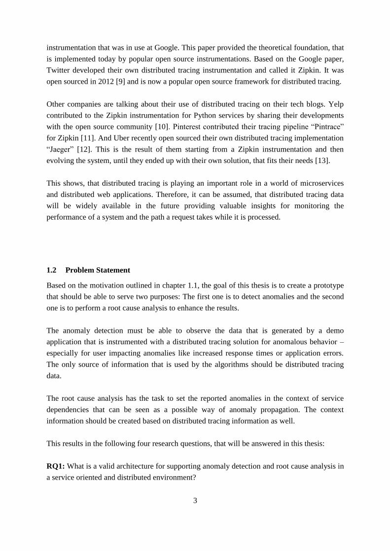
Figure 1: Differences in scaling between monoliths and microservices [14]
A Monolith shares memory and databases and is able to communicate through method calls
instead of messages. However, if you need to scale a monolithic application you cannot do
this on the service level as you can do with microservices, but you have to replicate the whole
monolith on another server. This is shown in Figure 1. Hence, this does not allow to scale as
flexible and efficient as in a microservice architecture. In addition, in a monolithic application
it is necessary to stick with a technology stack that is previously defined. Additionally, in the
case of an application update the whole applications needs to be recompiled and rebooted and
not only the affected service.
2.1.3 Differentiation from Service Oriented Architecture (SOA)
“SOA is focused on creating a design style, technology, and process framework that will
allow enterprises to develop, interconnect, and maintain enterprise applications and services
efficiently and cost-effectively.”[16] This characterization of the goals of SOA from
Papazoglou and van den Heuvel show the focus of SOA towards making the functionalities of
enterprise applications accessible as services.
One difference between Microservices and SOA are the completely different approaches
about how the structure of the application is looked at. For Microservices it is important to
have the component based and independent internal structure. In contrast, SOA just looks at
providing an integrated view of the underlying services to the outer world. For SOA it is not
important how the application or applications that deliver those services are built. [17]

8
Another differentiation of microservice architecture from SOA is the messaging approach
“smart endpoints and dumb pipes”. In contrast SOA often use an Enterprise Service Bus
(EBS) for communication. An EBS has internal routing logic for communication. This
contradicts the approach microservices take. There the smart logic is only inside the services
itself. [18]
2.1.4 Challenges for Microservice Architectures
Communication through messages is more expensive than method calls. Therefore, the
communication between services has to be optimized to the right level of granularity to enable
a high performance of the services. [14]
One challenge in microservice architectures is to handle failures gracefully. As each and
every service could go offline at any time, other services must be able to deal with such a
situation. Additionally, it is very important to detect those outages as fast as possible and
recover them [14]. However, the detection of anomalies is not an easy task, because
microservice architectures tend to change frequently. Therefore, calculating a baseline from
normal behavior to compare incoming data points against, is difficult [17].
As each functionality should be encapsulated in a separate microservice application, there are
a lot of applications to manage in a project. Enabling development, testing and deployment to
production for a large number of services requires a high degree of automation. Continuous
Integration with testing automation and a pipeline for Continuous Deployment are needed to
keep up with changes.[14]
2.1.5 Application in Practice
Microservice applications enable a company to react to changing business requirements in an
agile way. Additionally, they can be scaled very well, depending on the business needs.
Technical debt that has been accrued by companies in the past, prevents them from flexibly
adapting and scaling their applications. This is a reason why microservice architectures find
popularity in practice, supporting a new and flexible way forward. [19]
One of the early adopters of microservices in large scale was Netflix and the team around
Adrian Cockcroft. He migrated the companies monolithic application to an architecture with
hundreds of services that produce the streaming experience of the users today. [20]
Another big company that communicates openly about their migration to microservices is
Soundcloud. They state that switching to this architecture style enabled them to adopt their
development in a way, which decreases the effort of developing new services, set up
telemetry, testing and deployment of their applications. [21]

9
2.2 Distributed Tracing
In an application environment, where requests are processed by different services, it is no
longer enough to just look at the latency of the initial request. This might be enough to
identify that a problem exists, however there is no information on where this problem is
located. Using distributed tracing, information will be available that at least contains the begin
and end of each unit of work and where it was executed. This gives insight into the structure
of the application for a developer or operator – even if no deep knowledge about a system is
given or the system is changing frequently. With this information at hand, it is easier to
identify the root cause of a problem. [8]
When it comes to distributed tracing, the paper that is frequently cited as the basic idea for
current implementations is the work of Sigelman et al [8]. This paper describes Dapper, the
distributed tracing instrumentation that was in place at Google, when the paper was written.
One of the popular open source implementations for distributed tracing, OpenZipkin [22],
state that it is based on the Dapper paper. Compared to similar publications on the topic of
distributed tracing that are published without long production experience[23–25], the Dapper
publication includes insights and learnings from operating the system at a large scale.
The principal of the Dapper approach [8] is to instrument a commonly used library for
communication to track all incoming and outgoing requests and report them to a central
instance that aggregates the traces. This enables the instrumentation of an application without
the need of developers adhering to certain annotations. Every step that has to be done
repeatedly and manually could be forgotten which would impact the reliability of the
instrumentation. Furthermore, the less effort is required from the developers to integrate the
tracing into their application, the better the acceptance for distributed tracing will be.
Another publication on this topic is X-Trace [25]. In this concept, meta data is added to a
request to make it identifiable. This paper focuses on the possibility to track a request through
different administration domains (e.g. an Internet Service Provider and an Web Application
Provider) and on different protocol layers. The idea is that everyone can extract a trace for the
domain they are responsible for without sharing secrets with other domain owners. The
common identifier across all those domains gives the possibility to cooperate and
communicate with each other if need be. This approach requires to instrument all involved
clients and devices to include the metadata and to modify protocols to carry the meta data, if
they do not already have a possibility to do so.

10
Magpie [24] is another approach to distributed tracing. It uses a black box approach for
instrumenting the application to generate log files. Then an offline algorithm is used to derive
performance anomalies from an aggregated log. Pinpoint [23] is taking a similar approach to
Magpie, however focuses more on detecting faults.
Figure 2: Example Call Hierarchy
Figure 2 shows an example how a distributed call could look like. While the original call was
made to the service A, in the background services B-E are involved in processing the request,
before a result is returned.
Based on the Dapper paper [8], the terms of spans and traces have been coined. A span
represents a basic unit of work. This could be for example an HTTP request, that is sent from
the client to the server, processed on the server and the response returned to the client. When
looking at Figure 3, each execution will be represented by a span. A span has a begin and an
end timestamp. It has an Span ID and a Trace ID as reference to the trace it belongs to. Each
span, except the root of a trace, has a reference to its parent. And furthermore, the endpoint,
that generated the span can be identified. A trace is the tree of spans that are required to serve
a request. It starts at the border of the instrumented application, includes all calls to
instrumented services, that are needed for processing the request, and finishes once the
request leaves the instrumented application again. Those terms have found their way into the
terminology of open source implementations like OpenZipkin [22].

11
Figure 3: Simplified trace tree resulting from Figure 2
A widely used and open source implementation of Dapper [8] is OpenZipkin [22]. Originally
developed and open sourced by Twitter [9], it is now used by known companies such as
Pinterest [11] and Yelp [10]. Furthermore Uber recently open sourced their distributed tracing
framework Jaeger [12], that originated on OpenZipkin and then was modified to fit the
specific needs at Uber [13].
2.3 Anomaly Detection
The following section will focus on the topic of anomaly detection. First it will be explained
what anomalies are. Then metrics for anomaly detection are summarized. Afterwards possible
failure scenarios that result in anomalies are pointed out. And finally challenges and
application fields of anomaly detection are described.
2.3.1 What are anomalies?
A very early definition of an anomaly – in this case called outlier – is Hawkins definition
from 1980: An outlier is “an observation which deviates so much from other observations as
to arouse suspicions that it was generated by a different mechanism”[26].
Bovenzi et al[27] define an anomaly as “changes in the variable characterizing the behavior of
the system caused by specific and non-random factors”.

12
Anomaly detection in literature comes often in the context of failure prediction. Another term
that is frequently used is outlier detection. To define a more precise language for different
types of anomalies in time series data, the three categories defined by Laptev et al [28] will be
used in this thesis:
• An Outlier is a single data point in a time series. Its value deviates significantly from
the value that is expected at this point.
• A Changepoint is a point in a time series that marks the border where afterwards the
behavior of a time series is significantly different than before that point
• An anomalous time series deviates in its behavior significantly from others in a set of
time series that are expected to display similar behavior.
Figure 4: Artificial distribution of requests in regard to their duration to illustrate outliers.
Outliers in red circle.
Figure 4 illustrates how outliers can look like in a data set. It shows the distribution of the
number of requests in relation to their response time. The majority of the requests took
between 20ms and 50ms. The few requests further to the right with response times that are
higher than 120ms are deviating from what is usually expected. These requests would be
considered as outliers regarding their response time.
13
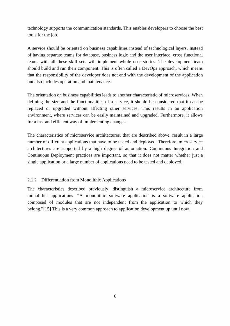
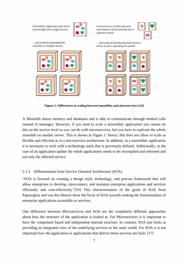
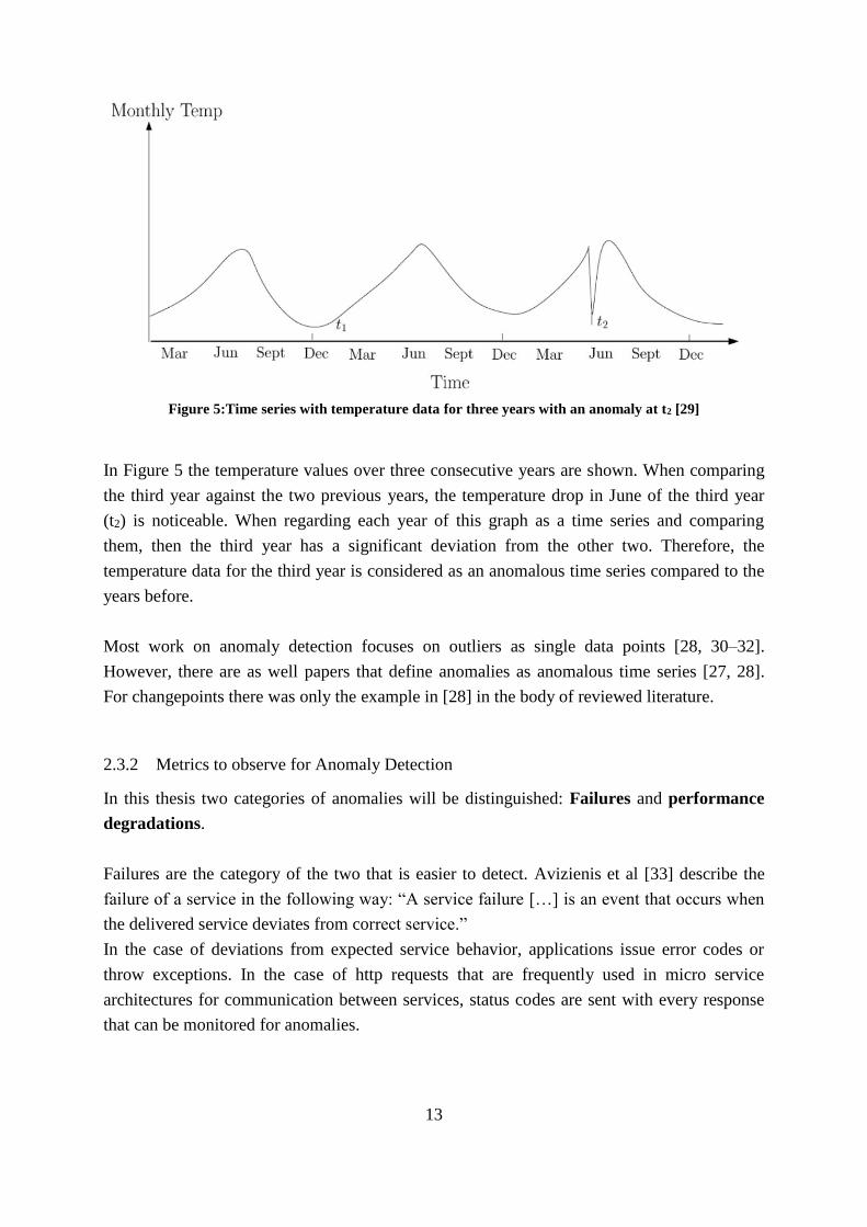
Figure 5:Time series with temperature data for three years with an anomaly at t2 [29]
In Figure 5 the temperature values over three consecutive years are shown. When comparing
the third year against the two previous years, the temperature drop in June of the third year
(t2) is noticeable. When regarding each year of this graph as a time series and comparing
them, then the third year has a significant deviation from the other two. Therefore, the
temperature data for the third year is considered as an anomalous time series compared to the
years before.
Most work on anomaly detection focuses on outliers as single data points [28, 30–32].
However, there are as well papers that define anomalies as anomalous time series [27, 28].
For changepoints there was only the example in [28] in the body of reviewed literature.
2.3.2 Metrics to observe for Anomaly Detection
In this thesis two categories of anomalies will be distinguished: Failures and performance
degradations.
Failures are the category of the two that is easier to detect. Avizienis et al [33] describe the
failure of a service in the following way: “A service failure […] is an event that occurs when
the delivered service deviates from correct service.”
In the case of deviations from expected service behavior, applications issue error codes or
throw exceptions. In the case of http requests that are frequently used in micro service
architectures for communication between services, status codes are sent with every response
that can be monitored for anomalies.
14
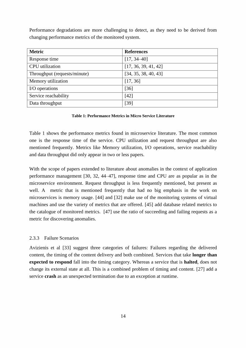
Performance degradations are more challenging to detect, as they need to be derived from
changing performance metrics of the monitored system.
Metric References
Response time [17, 34–40]
CPU utilization [17, 36, 39, 41, 42]
Throughput (requests/minute) [34, 35, 38, 40, 43]
Memory utilization [17, 36]
I/O operations [36]
Service reachability [42]
Data throughput [39]
Table 1: Performance Metrics in Micro Service Literature
Table 1 shows the performance metrics found in microservice literature. The most common
one is the response time of the service. CPU utilization and request throughput are also
mentioned frequently. Metrics like Memory utilization, I/O operations, service reachability
and data throughput did only appear in two or less papers.
With the scope of papers extended to literature about anomalies in the context of application
performance management [30, 32, 44–47], response time and CPU are as popular as in the
microservice environment. Request throughput is less frequently mentioned, but present as
well. A metric that is mentioned frequently that had no big emphasis in the work on
microservices is memory usage. [44] and [32] make use of the monitoring systems of virtual
machines and use the variety of metrics that are offered. [45] add database related metrics to
the catalogue of monitored metrics. [47] use the ratio of succeeding and failing requests as a
metric for discovering anomalies.
2.3.3 Failure Scenarios
Avizienis et al [33] suggest three categories of failures: Failures regarding the delivered
content, the timing of the content delivery and both combined. Services that take longer than
expected to respond fall into the timing category. Whereas a service that is halted, does not
change its external state at all. This is a combined problem of timing and content. [27] add a
service crash as an unexpected termination due to an exception at runtime.

15
In this thesis, we consider three possible failure scenarios:
• The service crashes due to a runtime exception
• The service does not return and the request times out eventually
• The service has an increased response time compared to normal operation
Memory leak is mentioned as a typical example of a failure scenario by Pitakrat et al [47] and
is also mentioned as a failure scenario by Lan et al [48]. They describe the pattern of this
scenario as follows: The heap utilization and the memory utilization are increasing in a linear
way. Once a certain threshold is passed, garbage collection kicks in heavily and increases
CPU utilization more and more. This results in poor performance of the application when
serving requests, with the result of increased response time.
Another failure scenario example described by Pitakrat et al [47] are failing requests. They
state that if the rate of succeeding requests falls below a certain threshold they consider this as
an anomaly. Furthermore, they are pointing out a scenario of system overload, where the
system cannot handle all the incoming requests in time. This might either result in increased
response times or into failing requests.
2.3.4 Anomaly Detection Algorithms
When reviewing literature, different approaches to algorithms for anomaly detection can be
found. Two major categories are machine learning approaches and statistical approaches
[44]. The machine learning approaches can further be separated into supervised and
unsupervised learning [32]. For supervised learning, there is a data set with labels for each
data point with the category (e.g. anomaly or normal behavior) it should be classified later on.
For unsupervised learning, you only get a set of data points without any additional knowledge
- it might contain normal data points as well as anomalies.
Outliers (as defined in chapter 2.3.1) can be either derived as exceeding an absolute value that
was previously defined (e.g. in a Service Level Agreement) or by exceeding a threshold above
a certain calculated baseline [45]. Those thresholds can be either static or adaptive [27].
Furthermore, you can do those predictions offline or online. This means either a data set is
collected and then processed offline in batches to determine whether those data points are
anomalies or not – or the predictions are performed online, once a data point arrives.
In the following, approaches to anomaly detection are explained, which will be considered
when selecting the algorithms for the prototype.
Clustering Based
One approach for anomaly detection is based on Clustering Algorithms [30, 44, 49]. In this
approach, first an arbitrary, but usually predefined number of cluster centers is calculated for

16
the data set. A commonly used algorithm for this step is KMeans Clustering [50]. The
assumption is, that the training set contains a set of normal data points. Then the distance
between each of the training set data points and its nearest cluster center is calculated. Those
distances are used to specify a value, that will be used as a threshold. If a data point is further
away from the nearest cluster center than this value, it is regarded as an outlier.
Computing the cluster centers and the thresholds can be very expensive, however for
predicting on incoming data points the computational effort is low. To predict whether an
incoming data point is an anomaly or not, it is enough to find the closest cluster center and
calculate the distance to it. Then this distance is compared to the threshold. If it is smaller, the
incoming data point is normal, otherwise it is classified as an anomaly.
Distance Based
The next approach is based on the number of neighbors within a specified distance to a certain
point in a dataset [48, 51, 52]. Those outliers are called distance based outliers and they are
defined as follows: “For the given positive parameters: k and R, an object o in data set D is a
DB(k, R, D)-outlier if the number of objects which lie within the distance of R from o is less
than k.”[51]
Due to this definition, the state of such an object can change, when new points are added. If
an object has already enough objects in its neighborhood, when it is inserted into the data set,
it can be regarded as a save inlier. It will never become an outlier, as long as no objects are
removed from the data set. However, when we look at an object that is originally an anomaly,
when it was entered to the data set, due to not enough neighbors within the specified distance,
this one could become normal eventually. If enough incoming objects are in the neighborhood
of the anomalous object, it will eventually fulfil the requirements and can then be classified as
normal.
When you are only interested in whether an incoming data points will be an anomaly or not,
this algorithm has no training time. The only thing necessary is the availability of the set of
already recorded data points. However, all data points have to be kept available during the
prediction phase and all the neighbors of incoming objects, that lie within the distance border,
have to be identified each time. This means, that more calculations have to be performed at
prediction time compared to the clustering based approach.
In order to improve the suitability of the original algorithm for online anomaly detection
scenarios, Lan et al [48] designed an approximation of the algorithm, to increase its
performance. They divide the object space into cells and only keep the object count per cell.
When a new object arrives, they check first whether in the cell it belongs into, the object
count is high enough to classify it as normal. If not, they add up the counts of the surrounding

17
cells, until they either reach the required object count, or they reach the cells that are further
away than the specified distance.
Density based / local
Another approach to detect outliers in a set of data points is the Local Outlier Factor (LOF),
introduced by Breunig et al [53]. This approach assigns a degree of “outlierness”, the LOF, by
comparing the density of the neighborhood of a data point with the density of its neighbors’
neighborhoods. This is done by calculating the distance to the k-th closest neighbor (k-
distance) from the point that is evaluated. Then the same is done for those k neighbors.
The LOF is calculated by dividing the k-distance of the evaluated point p by the average of
the k neighbors’ k-distances. With this calculated LOF for every point in the data set a
ranking can be created or all data points with a LOF above a certain threshold can be
considered as outliers. An intriguing feature of this algorithm is, that depending on how large
k is set, it is capable of handling multiple clusters with different densities in the data set and
still come up with good results for local outliers, even if the densities of those clusters vary
greatly.
Calculating the LOF requires the whole data set to be present and requires a recalculation of
the LOF values for each data point, once new data is inserted. As this algorithm was designed
for offline use, this was not an issue. However, for online anomaly detection usages this must
be considered. Furthermore, this algorithm does not need any labeled training set, so it is a
unsupervised approach.
Figure 6: Outlier-factors for points in a sample dataset [53]
Figure 6 shows an example how LOF works. On the left side, you see the distribution of the
data points. They are grouped into mainly 4 clusters with several outliers in between. On the

18
right side you see the same distribution, but with an added third dimension. This dimension
represents the calculated outlier score. The higher the column, the more the data point is seen
as an outlier.
Time series modelling
Laptev et al [28] suggest a framework for anomaly detection where they model time series
based on historic data and give a predicted value for a certain point in time. If the measured
value at this point in time deviates from the predicted value by a larger amount than a
predefined threshold, this data point is regarded as an outlier.
Their suggestions for algorithms to model the time series include ARIMA [54], Exponential
Smoothing [55], Kalman Filter [56] and State Space Models [57]. Pitakrat et al also use
ARIMA to forecast time series in their work [47].
Time series distribution
Solaimani et al [44] present a statistical approach to detect anomalous time series. For a
predefined time window, they categorize the values into a fixed number of bins. This
distribution is then compared against historical distributions using Goodness of Fit of
Pearson’s Chi Square method. If the incoming time series deviates significantly from a
defined number of previously observed normal time series, it will be classified as anomaly.
This approach is comparing time series against each other. It is not possible to define a single
outlier, but it points out a whole anomalous time series. This means, that this algorithm tries
to figure out, whether the occurrence of values that follow after each other over a certain
amount of time is distributed equally or not.
Pattern based
Watanabe et al [58] propose an approach to anomaly prediction based on message patterns.
Their algorithm does create a dictionary of patterns that might be the indicator of system
failures. When a new set of data comes in, it is compared against the pattern dictionary. Then
a failure probability is calculated based on the known patterns. If this probability is above a
certain threshold, a warning is issued.
Mdini et al [59] take the pattern approach from the other side. They define a normal pattern,
based on a training set. Then they compare the incoming data against this base pattern. If the
incoming data deviates too much from the normal pattern, it will be regarded as an anomaly.
Neural Networks
Malhotra et al [60] chose Neural Networks to detect anomalous sequences in time series.
Specifically, they use Long Short Term Memory (LSTM) Neural Networks. Those Neural

19
Networks have a long term memory, that allows for discovering long term correlations in a
sequence. The Neural network is trained with a training set of sequences. Based on a
validation set, the trained model is used to calculate error vectors that are modelled towards a
Gaussian distribution. This distribution is then used to calculate a likelihood to observe a
certain error vector at a certain point in a sequence. If this likelihood drops below a certain
value, this part of a sequence is regarded anomalous.
By using this approach, they showed that they can train a model with normal behavior and
then detect sequences in a time series that do not match this normal behavior. They claim that
the advantage over other methods to predict anomalous time series sequences is, that this
approach does not need a specified sequence length or any preprocessing.
2.3.5 Challenges of Anomaly Detection for System Monitoring
Monitoring a micro service application to detect anomalies provides several challenges. The
task of an online monitoring application is to detect the occurring anomalies in real time [27].
Furthermore, it should be considered that a system that raises too many false alarms will
likely be turned off by the operator [61]. Therefore, a reliable detection algorithm that
supports online prediction is very important.
In a frequently changing application environment, like an evolving microservice application,
it is essential that the anomaly detection model is adapting frequently [47]. When the state of
the system at run time starts to deviate heavily from the state of the system, the detection
model was trained on, the accuracy of detecting anomalies decreases [27]. Therefore, it is
important to apply algorithms that cope with changing environments.
2.3.6 Application Fields of Anomaly Detection
Besides application monitoring, anomaly detection is used in many different areas. Popular
applications are in the fields of Intrusion Detection and Fraud Detection. Additionally, Sensor
Networks, Image Processing and Text Processing are areas where different kinds of anomaly
detection can be applied. [29]
2.4 Root Cause Analysis
In large scale distributed systems, it can be a huge effort to figure out the service that is
causing the observed anomalies. If a distributed application provides a large number of
services with a number of endpoints on each, there are a lot of locations, where a service

20
could actually behave anomalous. If the root cause for an anomaly, that was observed at one
of those endpoints, should be discovered, it gets even more complex, as services call each
other during the processing of their requests.[2]
Enhancing an anomaly detection system with information on services causing the detected set
of anomalies, can be of great use to pin down and solve the problems in a system as fast as
possible. This can be crucial, as appearing anomalies can really impact the business results of
a company, if it degrades the customer experience.
One possible approach is to take the architecture and the propagation of errors into account to
improve the anomaly prediction results [47]. Error propagation means, that when a specific
service A delivers an incorrect result to service B that was calling it, service B will continue
its calculation with the incorrect result and therefore deliver incorrect results as well [33, 47].
Even though service A and B will both deliver wrong results, the root cause of those
deviations is in service A. This means, that anomalies would be observed on both service A
and B, but service B is actually working correctly – just using the anomalous input from A.
The same propagation chain can happen for performance issues. If one service takes longer to
process a request than usual, this decrease in performance will be affecting all services that
rely on it.
Cortellessa et al [62] propose a modelling approach to improve the reliability of component
based systems during development. Based on the error propagation probability among
components, they draw conclusions of the reliability of the system. This approach tries to
discover possible root causes for errors at the time of system design and development and
mitigate their impact as far as possible.
Knowledge about root causes is of interest in a lot of different domains. Weng et al [63]
propose a solution for public cloud providers with multiple tenants, that shows root causes
that could either be a bug in a service itself or propagations from other tenants. Zasadzinski et
al [64] apply root cause analysis to the domain of the Internet of Things. And Gonzalez et al
[65] use root cause analysis in a network operation setting. All those fields of application have
in common, that a large amount of monitored devices or services are present and a manual
identification of the root cause from a set of anomalies is not feasible.

21
3 Solution Architecture
In the following, the process behind designing the architecture of the prototype will be
described. The architecture of the prototype is shown and afterwards, the key technologies are
explained in more detail.
3.1 Anomaly detection and root cause analysis pipeline design
The goal is to detect anomalies based on distributed tracing information. The specific
anomalies that should be detected are:
1. Increased response time compared to a learned baseline
2. Violations of a defined threshold
3. Errors
Furthermore, the detected anomalies should be set into the context of the architecture to
determine which reported anomalies are really coming from an anomalous service and which
ones are only suffering from error propagations.
The process can be described in the following five stages that are displayed in Figure 7.
Figure 7: Five Stage of the Anomaly and Root Cause Discovery Process
In the first stage, the data is extracted from the application through distributed tracing and
made available for later stages. Then the data is prepared to match the needs of the anomaly
detection algorithms. Those algorithms detect anomalies from the information, as soon as it
gets available – this means the data is streamed and processed online. Afterwards, the
detected anomalies are processed by the root cause analysis, to prioritize all anomalies that are
most likely root causes of a set of anomalies and deprioritize those that are caused by anomaly
propagation.

22
The prototype covers all these stages. However, the focus of this thesis is on preparing the
data, detecting anomalies and set them into a service dependency context to identify the root
cause of an anomaly. Data extraction must deliver the required features and visualization
should provide a basic overview of a previously modelled request to the monitored
application.
As this prototype is foreseen as the foundation for further research, to set it up for future use
and changes is essential. As already foreseeable, the system should be capable of evolving
over time to match changes in the direction of future research. A modular approach is the way
to go.
First and foremost, the models and algorithms for anomaly detection have to be exchangeable.
Even running different algorithms in parallel and still make good use of the results should be
possible. To achieve this, asynchronous message queues will be used for the communication
of distributed tracing, anomaly detection and root cause analysis. As parallel running
algorithms might all report the same request as anomalous, the root cause analysis must be
capable of identifying and merging those duplicates.
The other modular part should be the whole pipeline itself. Using a different instrumentation
to gather the distributed tracing, or deciding on a different approach to get the dependency
information for the root cause analysis should be possible without impacting the other parts.
As long as the message format stays the same, the modules should be exchangeable.
3.2 Architecture Overview
The architecture of the prototype and the choices of technologies to implement this pipeline is
shown in Figure 8 and is explained in the following. The main technologies will be described
in more detail in the next chapter.
The instrumentation of the application will be done based on Spring Cloud Sleuth. The basic
setup will be enhanced by some custom coded extensions to get access to additional
information that is useful for anomaly detection.
The distributed tracing data will be written to a Kafka topic in JSON format. This is where the
anomaly detection module, that is based on Apache Spark, collects its data from. The data is
extracted from Kafka and used in the different algorithms for anomaly detection, that run
within the module. Each of those algorithms is independent. It may or may not have a training

23
phase where it could access the whole historical data that is stored in Kafka at training time.
Each algorithm has a detection phase, when it looks at the incoming data points and evaluates
whether the data point is an anomaly or not. Each of the algorithms writes its detected
anomalies to a common anomaly topic in Kafka. Duplicates could occur, if the same data
point is reported by multiple algorithms.
Figure 8: Architecture Overview
The second module based on Apache Spark is the root cause analysis. It reads the detected
anomalous data points from Kafka and has the goal to report the root cause for a set of
anomalies. This is done by setting the reported anomalies into a context, representing how
anomalies are propagated among the services.
Finally, a simple visualization is implemented to help presenting the results of the system in a
more human readable way. However, as another thesis in this research project deals with the
specific topic of an intelligent user interface, this thesis will keep the visualization minimal.
3.3 Main Technologies
The following chapter describes the most important technologies that are used for the
prototype. Spring Cloud Sleuth is used for distributed tracing. Apache Spark provides the
24
foundation for the anomaly detection and root cause analysis. Apache Kafka is the
asynchronous messaging queue that is used for the communication between the modules.
3.3.1 Spring Cloud Sleuth
Spring Cloud Sleuth [66] is a distributed tracing framework for Spring Cloud Applications.
The demo application to be monitored(see chapter 6.1 for closer description) is already
instrumented with OpenZipkin [22]. Hence, it was already clear, that this would be used for
the distributed tracing.
The only decision that had to be made was at which level to pull the data. OpenZipkin relies
on the distributed traces, that are generated by Spring Cloud Sleuth. This framework is the
convenient and easy way to setup OpenZipkin for Spring Cloud applications by simply
adding a set of maven dependencies. One possibility was to read the traces from the database
that is kept by the Zipkin server. The other option is to get the data directly from the same
message queue, the Zipkin server reads the data from. The options of usable message queues
are Apache Kafka [67] and RabbitMQ [68]. As the goal of this prototype is performing online
anomaly detection, the message queue approach with plain Spring Cloud Sleuth is chosen as
the way to go. It promises to get the data without any postprocessing and as fast as possible.
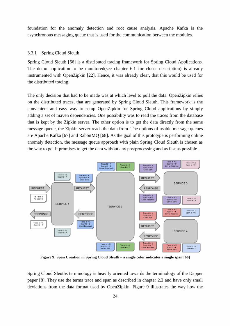
Figure 9: Span Creation in Spring Cloud Sleuth – a single color indicates a single span [66]
Spring Cloud Sleuths terminology is heavily oriented towards the terminology of the Dapper
paper [8]. They use the terms trace and span as described in chapter 2.2 and have only small
deviations from the data format used by OpenZipkin. Figure 9 illustrates the way how the
25
spans of a trace are recorded. A common color indicates which information belongs together
as a span in the sense of the definition in the Dapper paper. However, when looking for
example at the blue spans with the Span ID = B, it already shows a difficulty. The one part of
the span is recorded in one service and the other part in another service.
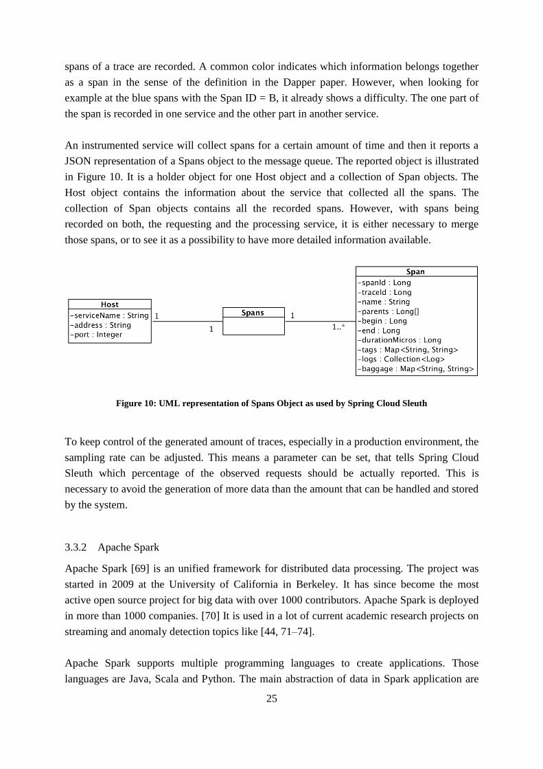
An instrumented service will collect spans for a certain amount of time and then it reports a
JSON representation of a Spans object to the message queue. The reported object is illustrated
in Figure 10. It is a holder object for one Host object and a collection of Span objects. The
Host object contains the information about the service that collected all the spans. The
collection of Span objects contains all the recorded spans. However, with spans being
recorded on both, the requesting and the processing service, it is either necessary to merge
those spans, or to see it as a possibility to have more detailed information available.
Figure 10: UML representation of Spans Object as used by Spring Cloud Sleuth
To keep control of the generated amount of traces, especially in a production environment, the
sampling rate can be adjusted. This means a parameter can be set, that tells Spring Cloud
Sleuth which percentage of the observed requests should be actually reported. This is
necessary to avoid the generation of more data than the amount that can be handled and stored
by the system.
3.3.2 Apache Spark
Apache Spark [69] is an unified framework for distributed data processing. The project was
started in 2009 at the University of California in Berkeley. It has since become the most
active open source project for big data with over 1000 contributors. Apache Spark is deployed
in more than 1000 companies. [70] It is used in a lot of current academic research projects on
streaming and anomaly detection topics like [44, 71–74].
Apache Spark supports multiple programming languages to create applications. Those
languages are Java, Scala and Python. The main abstraction of data in Spark application are
26
RDDs (Resilient Distributed Datasets). They are collections of objects that can be distributed
across multiple clusters for fast parallel processing of tasks. The basic operations to transform
the data are map, filter and group by operations.
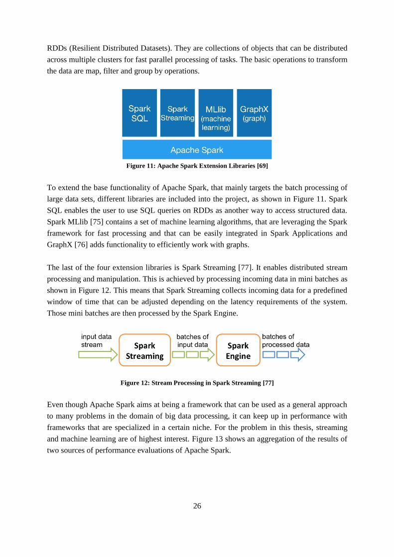
Figure 11: Apache Spark Extension Libraries [69]
To extend the base functionality of Apache Spark, that mainly targets the batch processing of
large data sets, different libraries are included into the project, as shown in Figure 11. Spark
SQL enables the user to use SQL queries on RDDs as another way to access structured data.
Spark MLlib [75] contains a set of machine learning algorithms, that are leveraging the Spark
framework for fast processing and that can be easily integrated in Spark Applications and
GraphX [76] adds functionality to efficiently work with graphs.
The last of the four extension libraries is Spark Streaming [77]. It enables distributed stream
processing and manipulation. This is achieved by processing incoming data in mini batches as
shown in Figure 12. This means that Spark Streaming collects incoming data for a predefined
window of time that can be adjusted depending on the latency requirements of the system.
Those mini batches are then processed by the Spark Engine.
Figure 12: Stream Processing in Spark Streaming [77]
Even though Apache Spark aims at being a framework that can be used as a general approach
to many problems in the domain of big data processing, it can keep up in performance with
frameworks that are specialized in a certain niche. For the problem in this thesis, streaming
and machine learning are of highest interest. Figure 13 shows an aggregation of the results of
two sources of performance evaluations of Apache Spark.
27
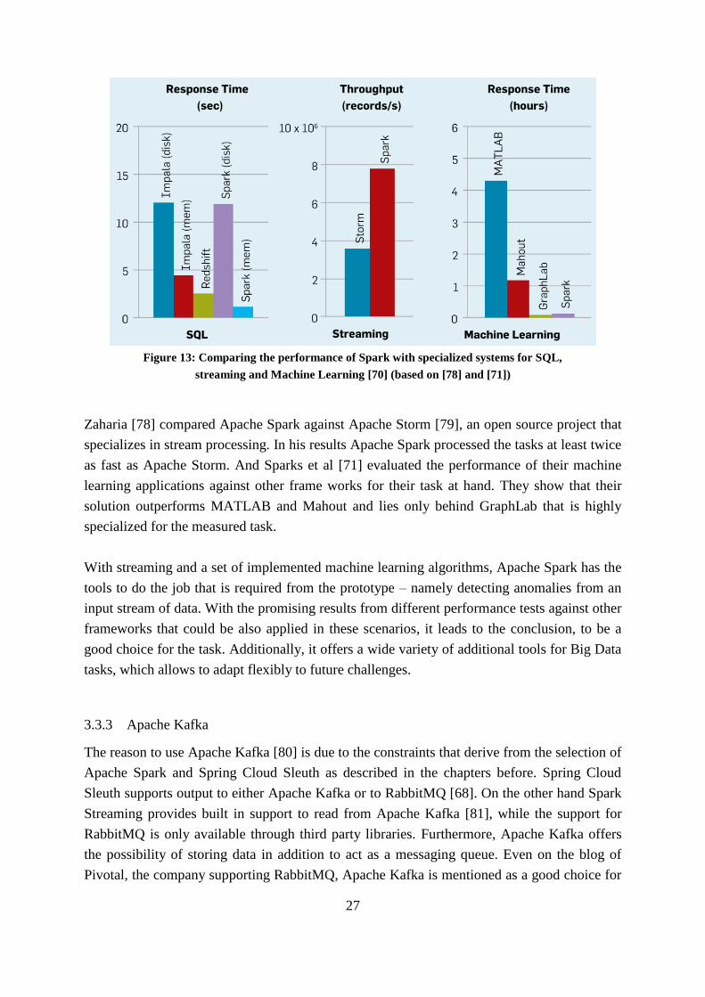
Figure 13: Comparing the performance of Spark with specialized systems for SQL,
streaming and Machine Learning [70] (based on [78] and [71])
Zaharia [78] compared Apache Spark against Apache Storm [79], an open source project that
specializes in stream processing. In his results Apache Spark processed the tasks at least twice
as fast as Apache Storm. And Sparks et al [71] evaluated the performance of their machine
learning applications against other frame works for their task at hand. They show that their
solution outperforms MATLAB and Mahout and lies only behind GraphLab that is highly
specialized for the measured task.
With streaming and a set of implemented machine learning algorithms, Apache Spark has the
tools to do the job that is required from the prototype – namely detecting anomalies from an
input stream of data. With the promising results from different performance tests against other
frameworks that could be also applied in these scenarios, it leads to the conclusion, to be a
good choice for the task. Additionally, it offers a wide variety of additional tools for Big Data
tasks, which allows to adapt flexibly to future challenges.
3.3.3 Apache Kafka
The reason to use Apache Kafka [80] is due to the constraints that derive from the selection of
Apache Spark and Spring Cloud Sleuth as described in the chapters before. Spring Cloud
Sleuth supports output to either Apache Kafka or to RabbitMQ [68]. On the other hand Spark
Streaming provides built in support to read from Apache Kafka [81], while the support for
RabbitMQ is only available through third party libraries. Furthermore, Apache Kafka offers
the possibility of storing data in addition to act as a messaging queue. Even on the blog of
Pivotal, the company supporting RabbitMQ, Apache Kafka is mentioned as a good choice for

28
scenarios where a “stream from A to B without complex routing, with maximal throughput”
[82] is required. And this is exactly what is needed for this prototype. Therefore, Apache
Kafka is chosen as tool for the job of asynchronous messaging.
Figure 14: Apache Kafka Architecture [80]
Apache Kafka acts as a publish/subscribe messaging queue while on the same time storing the
data and keeping it available based on a setup retention policy. The most important roles in
the Kafka architecture are producers, brokers and consumers. As shown in Figure 14,
applications that act as producers, send data to the Kafka Cluster. The cluster acts as broker,
that administrates the different topics. A topic is the destination, where the producer writes its
messages to and where the consumers can subscribe to, to receive all the new incoming
messages. A consumer that subscribes to a topic can decide to first receive all messages, that
are currently stored in the topic or not to receive the historical messages and just read the new
incoming messages. To ensure that no data is lost due to the failure of a node in the Kafka
Cluster, the topics can be replicated among the nodes.
29
4 Anomaly Detection
When looking at the detection of anomalies there are the three scenarios described in chapter
2.3.3 that the prototype should be able to detect. First, errors have to be detected. In this case
the monitored application does not process the request as expected, but returns an error code
or an exception. The second case are timeouts. A request is sent to the application but there is
never a response returned and eventually the application throws a timeout exception. And
finally, the prototype has to detect performance problems. This is the case when the
application does not process the requests as fast as it usually does.
In the following chapter, it will be explained which parameters can be collected with the
distributed tracing instrumentation. Afterwards the selection of the algorithms for the
prototype is explained. And finally, the implementation will be described.
4.1 Feature Extraction
In chapter 2.3.2 common metrics were collected that have been used in current research to
identify anomalies. Namely those are response time, CPU utilization, memory utilization and
throughput in requests per minute.
As described earlier, Spring Cloud Sleuth [66] is used to instrument the microservices and
extract information about requests. The only metric that is implemented by default is the
response time. More precisely the duration of the span that is representing a request.
By customizing the framework, CPU utilization average over the last minute and heap
memory utilization of the Java Virtual Machine (JVM) are added to the extracted
parameters. Those changes are based on monitoring possibilities from inside the JVM and do
only require developers to add a few lines of code once they set up a microservice in a single
place. Listing 1 shows all that needs to be done on each service in the configuration class.
After injecting a BeanFactory and the Spring Cloud Sleuth Tracer, three beans have to be
registered. Those beans are imported through a maven dependency. After set-up, no more
additional code is required, for the distributed tracing instrumentation to work. This keeps the
implementation effort minimal and is ensuring that the instrumentation cannot be forgotten
during the application development process. Furthermore, it is easy to instrument an already
existing application, without the need to modify a lot of code.

30
@Configuration public class MvcConfig extends WebMvcConfigurerAdapter { Tracer tracer; @Autowired BeanFactory beanFactory; Tracer tracer() { if (this.tracer == null) { this.tracer = this.beanFactory.getBean(Tracer.class); } return this.tracer; } @Bean
public CustomTraceHandlerInterceptor customTraceHandlerInterceptor(BeanFactory beanFactory) {
return new CustomTraceHandlerInterceptor(beanFactory, tracer()); } @Bean public SpanAdjuster customSpanAdjuster() { return new CustomSpanAdjuster(); } @Bean CustomFilter customFilter() { return new CustomFilter(tracer()); } }
Listing 1: Once required Code per Service to implement the enhanced tracing
instrumentation
On top of the metrics suggested in literature, Spring Cloud Sleuth offers some more features
to look at. There is some useful information to map the request to specific method calls on a
specific instance of a service. This information includes the request’s URI, service-name
and IP address and port of the service host.
For http requests, that are an important means of communication for microservices, there is
further information available. The HTTP method and HTTP status are reported by Spring
Cloud Sleuth. Furthermore, in case of an error, an additional error tag is set once in a trace,
reporting the error message of the exception thrown. If the reported span is no http request,
but representing a request that is processed by a controller, the controller class name and
method name are available.
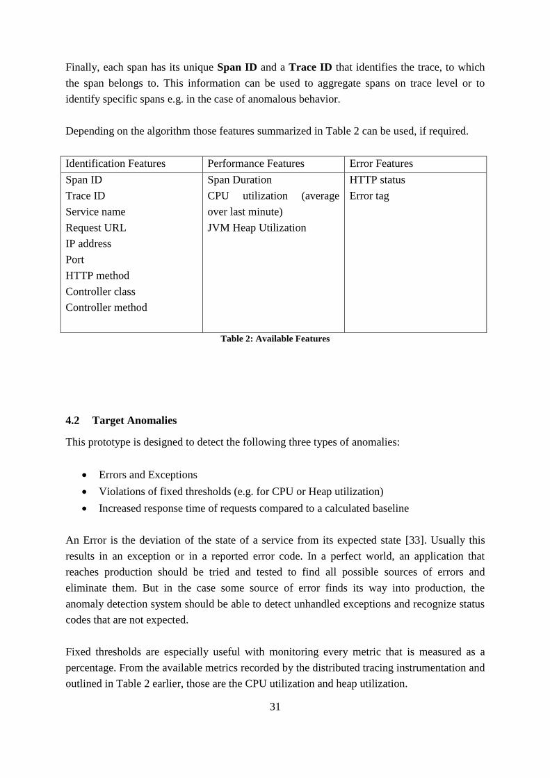
31
Finally, each span has its unique Span ID and a Trace ID that identifies the trace, to which
the span belongs to. This information can be used to aggregate spans on trace level or to
identify specific spans e.g. in the case of anomalous behavior.
Depending on the algorithm those features summarized in Table 2 can be used, if required.
Identification Features Performance Features Error Features
Span ID
Trace ID
Service name
Request URL
IP address
Port
HTTP method
Controller class
Controller method
Span Duration
CPU utilization (average
over last minute)
JVM Heap Utilization
HTTP status
Error tag
Table 2: Available Features
4.2 Target Anomalies
This prototype is designed to detect the following three types of anomalies:
• Errors and Exceptions
• Violations of fixed thresholds (e.g. for CPU or Heap utilization)
• Increased response time of requests compared to a calculated baseline
An Error is the deviation of the state of a service from its expected state [33]. Usually this
results in an exception or in a reported error code. In a perfect world, an application that
reaches production should be tried and tested to find all possible sources of errors and
eliminate them. But in the case some source of error finds its way into production, the
anomaly detection system should be able to detect unhandled exceptions and recognize status
codes that are not expected.
Fixed thresholds are especially useful with monitoring every metric that is measured as a
percentage. From the available metrics recorded by the distributed tracing instrumentation and
outlined in Table 2 earlier, those are the CPU utilization and heap utilization.

32
The third type of anomalies is the increased response time compared to a baseline. As
explained in the motivation for this thesis (Chapter 1.1), increased response times can have a
negative impact on the success of a business running a web application. Therefore, a baseline
should be established. Increased response time anomalies will be all requests, that exceed the
calculated base value by more than a certain threshold.
With detecting those types of anomalies, it is possible to detect the failure scenarios, that were
described in chapter 2.3.3:
• The service crashes due to a runtime exception
• The service does not return and the request times out eventually
• The service has an increased response time compared to normal operation
The first scenario will cause an error or an exception, that is one of the defined anomalies
above. By detecting those, this scenario is covered.
In the monitored system, a request that takes too long, will cause the system to throw a
timeout exception. Hence, this failure scenario is as well covered by the error detection. If
another system handles a timeout by returning a request with a very long request duration, this
would be covered by the detection of increased response times. The only case that cannot be
detected by the system, is a case where nothing is reported. If there is no reported span to
predict on, the system will not be able to detect anything.
To illustrate the usefulness of the Fixed Threshold monitoring, the memory leak scenario, that
was mentioned as an example for a failure in chapter 2.3.3, will be used. In this scenario CPU
usage usually increases, when the JVM heap utilization is above a certain threshold. This is
due to the fact that in this case the garbage collector activity is increasing heavily [47]. If a
system operator knows, where this heap threshold for his system is, he can set this threshold
and will be informed, once a certain service enters such a critical zone. Furthermore, fixed
thresholds could be used to monitor compliance to negotiated service level agreements.
4.3 Algorithm Selection
In the following, the selection of the algorithms for detecting the three types of anomalies that
were pointed out in the previous section is explained. The approaches, that are considered for
this selection were described in chapter 2.3.4.

33
Monitoring for errors and timeouts does not require any machine learning or statistical
algorithm in the use case at hand. When an exception is thrown, Spring Cloud Sleuth attaches
an error tag to the current span. Furthermore, spans for HTTP requests get a tag with the http
status that is returned. Therefore, filtering for spans with error tags or an HTTP status of 500
(Internal Server Error) will result in a stream of spans where requests have either timed out –
then a timeout exception is thrown – or have provoked an unhandled exception in the
application. This is comparable to the pattern based approach. However, no learning is in
place. Just a pattern, that is known to be anomalous, will be detected.
When monitoring for performance anomalies, the three metrics JVM memory utilization,
CPU utilization and request duration are available from the instrumentation. To make best use
of the available information those metrics can be treated differently.
The JVM memory utilization is a metric that can be used as early indicator that something
could go wrong. As garbage collection kicks in more frequently, when heap space is running
out [47], it is beneficial to set up an anomaly warning, when heap space utilization exceeds a
certain threshold.
As the CPU utilization is reported as a percentage, the easiest way to report anomalies is by
defining a fixed threshold that is regarded as being an anomaly and compare the incoming
values of this metric against this threshold.
Compared to memory and CPU utilization the threshold for the duration is trickier to define.
As the expected duration varies from endpoint to endpoint, a predefined threshold is not an
option. It is necessary to derive a baseline and an acceptable threshold from normal behavior
data of the system and use that to detect anomalies.
As the system aims to do online anomaly detection, it is paramount, that the algorithms will
be capable of processing incoming data points very fast to deliver results in a timely manner
and to be able to handle a large amount of incoming data. In addition, it has to be considered,
that each endpoint behaves differently. Therefore, it is likely, that it could be necessary to
store a trained model for each endpoint to detect the anomalies. This requires the algorithm to
store the information that is needed for each endpoint in a way that is as minimal as possible.
To ensure fast and well-fitting implementation, it would be very beneficial to have support for
the chosen algorithm through Spark MLlib. It would be beneficial to have a sufficient amount
of documentation, to get started fast.
As the system is designed in a way, that multiple algorithms can be run in parallel. This
means, that new algorithms can be placed alongside the originally implemented algorithms or

34
replace them entirely. As the system is designed to evolve during further research, the
selected algorithm does not have to be perfect – but it has to be capable of performing the task
of detecting increased response times effectively.
Furthermore, the algorithm has to detect outliers. As the root cause analysis implementation
(described in chapter 5.2) is based on the assumption, that the anomalies are predicted on span
level. Therefore, it is not possible to use an algorithm that detects anomalous time series, as
then the information on span level that are needed for the root cause analysis would be lost.
The density based approach using LOF can be ruled out, as it is not efficient during
prediction. This counts as well for the exact distance based approach. The cell based version
should be efficient enough, however there is no implementation available in the collection of
MLlib algorithms and no popular third party library.
The time series distribution approach is only working for detecting anomalous time series.
This means, that it will be difficult to identify the required anomalous spans for the root cause
analysis.
This leaves an approach based on time series modelling or on clustering. For the first one,
there is no support in Spark MLlib directly and the third party library [83], that is pointed to
in different communities, is no longer under active development and has only few
documentation and examples. For clustering however, there is an implementation of the
popular KMeans algorithm available directly in MLlib. This approach has furthermore the
advantage, that after the training phase, anomaly detection is very efficient and the only
information that has to be stored for each endpoint are the coordinates of the calculated cluster
centers and the threshold distance. Hence, the algorithm in the prototype for detecting
increased response times will be developed based on clustering.
4.4 Implementation
The following chapter describes the implementation of the anomaly detection process of the
prototype. It will start with describing the faced challenges. The overview of the anomaly
detection pipeline follows, before the different parts of the anomaly detection process are
broken down in more detail.
4.4.1 Challenges
The first challenge that must be addressed is the fact, that there is no information about the
monitored system available up front. As the anomaly detection should work with any

35
application, that implements the distributed tracing information, the only available knowledge
up front is the behavior of Spring Cloud Sleuth in presence of certain events.
The next requirement for the system is to detect anomalies in real time. This means, that the
data has to be categorized as normal or not, as soon as it is available. Calculating a baseline
however, is acceptable to be performed before starting the anomaly detection.
Furthermore, this prototype is restricted to only use data available from distributed tracing. In
literature, often hardware sensors are used to gather for example CPU information. The
developed prototype is restricted to work with the information that is available from using
Spring Cloud Sleuth. Out of the box that would only be information on the duration of a span
and the information to locate the appropriate service and method, where this span was
reported. However, as described in section 4.1, by using the customization option of Spring
Cloud Sleuth, additional instrumentations have been implemented to gather information on
JVM heap utilization and the average CPU utilization over the last minute.
Finally, the module for anomaly detection must support the modular approach that was set
when designing the system. This requires asynchronous communication to the distributed
tracing information before and the root cause analysis after it in the pipeline using Kafka
topics. Furthermore, the algorithms used for anomaly detection should be implemented in a
way, that multiple algorithms can run in parallel and implementing a new algorithm to add to
the pipeline should be easily feasible.
4.4.2 Pipeline Overview
The basic concept to implement the detection of the three anomaly types described above, is
shown in Figure 15. A commonly used module is implemented for extracting the information
from Kafka – the basic process is equal for all three algorithms. The anomaly reporting is
similar for all algorithms as well – in the end all anomalies have to be reported to the same
Kafka topic in a predefined and common format.
Figure 15: Anomaly Detection Pipeline Concept

36
The application is developed in a way, that an arbitrary number of anomaly detection
algorithms can be installed and run in parallel. They could try to detect similar anomalies or
completely different ones – as long as they do it based on the spans, the import provides.
Interpreting those reported anomalous spans is then the task of the root cause analysis.
In the following, the single steps of the anomaly detection pipeline will be explained in more
detail.
4.4.3 Data Import
Before any of the anomaly detection algorithms can start their individual processing, the
Spark Application needs access to the data that has been reported by the distributed tracing
instrumentation and is stored in Kafka by the Spring Cloud Sleuth instrumentation. The topic
contains JSON representation of the Spring Cloud Sleuth Spans object, as shown in Figure 10
in chapter 3.3.1. It is a container for information about a set of reported spans and the service
and endpoint, that did report them. The JSON representation is preceded by additional header
information.
The most interesting information is found in the Span objects. Especially the duration and the
tags, that represent attributes that can be set to a span, will be used by the anomaly detection
algorithms. The IDs, name and host information will serve as a way to identify and group the
requests, that are represented by those spans, by the endpoints they were reported by. An
endpoint is the combination of host, service and method. It identifies the location, where a
span was created.
To create the initial stream with the input from the Kafka topic, Apache Spark Streaming,
which is used for the implementation of the anomaly detection, makes use of a connector
library [81]. After the stream is opened, it can be manipulated with mapping and filter
operations.
In a first step, the header information is removed, so the remainder only contains the JSON.
Afterwards the JSON is converted into Spring Cloud Sleuth’s Spans object for easier
processing.
However, as the anomalies will be detected on span level, they must be extracted from the list
inside the Spans object. After extracting the single Span objects, they are mapped together
with the corresponding Host object as a tuple. This is done to retain the host information
throughout the anomaly detection process. The resulting tuple stream is the basis on which
each of the algorithms, that are described in the following chapters 4.4.4 - 4.4.6 will start their
stream manipulations and calculations.
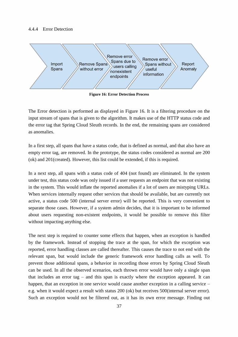
37
4.4.4 Error Detection
Figure 16: Error Detection Process
The Error detection is performed as displayed in Figure 16. It is a filtering procedure on the
input stream of spans that is given to the algorithm. It makes use of the HTTP status code and
the error tag that Spring Cloud Sleuth records. In the end, the remaining spans are considered
as anomalies.
In a first step, all spans that have a status code, that is defined as normal, and that also have an
empty error tag, are removed. In the prototype, the status codes considered as normal are 200
(ok) and 201(created). However, this list could be extended, if this is required.
In a next step, all spans with a status code of 404 (not found) are eliminated. In the system
under test, this status code was only issued if a user requests an endpoint that was not existing
in the system. This would inflate the reported anomalies if a lot of users are mistyping URLs.
When services internally request other services that should be available, but are currently not
active, a status code 500 (internal server error) will be reported. This is very convenient to
separate those cases. However, if a system admin decides, that it is important to be informed
about users requesting non-existent endpoints, it would be possible to remove this filter
without impacting anything else.
The next step is required to counter some effects that happen, when an exception is handled
by the framework. Instead of stopping the trace at the span, for which the exception was
reported, error handling classes are called thereafter. This causes the trace to not end with the
relevant span, but would include the generic framework error handling calls as well. To
prevent those additional spans, a behavior in recording those errors by Spring Cloud Sleuth
can be used. In all the observed scenarios, each thrown error would have only a single span
that includes an error tag – and this span is exactly where the exception appeared. It can
happen, that an exception in one service would cause another exception in a calling service –
e.g. when it would expect a result with status 200 (ok) but receives 500(internal server error).
Such an exception would not be filtered out, as it has its own error message. Finding out
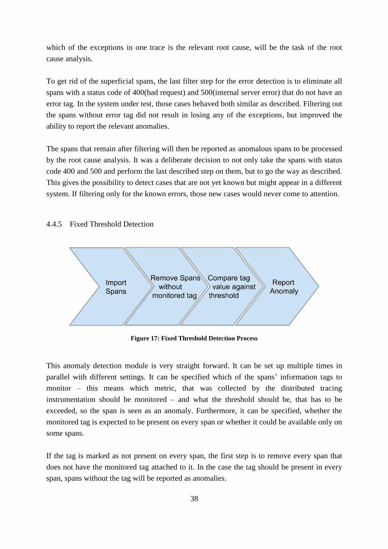
38
which of the exceptions in one trace is the relevant root cause, will be the task of the root
cause analysis.
To get rid of the superficial spans, the last filter step for the error detection is to eliminate all
spans with a status code of 400(bad request) and 500(internal server error) that do not have an
error tag. In the system under test, those cases behaved both similar as described. Filtering out
the spans without error tag did not result in losing any of the exceptions, but improved the
ability to report the relevant anomalies.
The spans that remain after filtering will then be reported as anomalous spans to be processed
by the root cause analysis. It was a deliberate decision to not only take the spans with status
code 400 and 500 and perform the last described step on them, but to go the way as described.
This gives the possibility to detect cases that are not yet known but might appear in a different
system. If filtering only for the known errors, those new cases would never come to attention.
4.4.5 Fixed Threshold Detection
Figure 17: Fixed Threshold Detection Process
This anomaly detection module is very straight forward. It can be set up multiple times in
parallel with different settings. It can be specified which of the spans’ information tags to
monitor – this means which metric, that was collected by the distributed tracing
instrumentation should be monitored – and what the threshold should be, that has to be
exceeded, so the span is seen as an anomaly. Furthermore, it can be specified, whether the
monitored tag is expected to be present on every span or whether it could be available only on
some spans.
If the tag is marked as not present on every span, the first step is to remove every span that
does not have the monitored tag attached to it. In the case the tag should be present in every
span, spans without the tag will be reported as anomalies.

39
After this filter step, the value from the tag will be extracted. This value is then compared to
the threshold that was defined previously. If the value exceeds the threshold, the span will be
reported as an anomalous span for further processing by the root cause analysis.
4.4.6 Splitted KMeans – Increased Response Time Detection
The most complex algorithm for anomaly detection in this prototype is the one to detect
increased response times. This algorithm has a training phase, once it is started to create a
baseline and a threshold. Then the anomaly detection phase kicks in, where the result from the
training phase is used to detect anomalies in the stream of incoming spans.
Training phase
For the training phase, a set of historic data is needed. In this case Kafka’s storage
functionality is very useful. Kafka stores all the data of a topic based on a defined retention
policy. When a new client starts to read from a topic it has two possibilities. The first is to
receive everything that is written to that topic after the client subscribed. The other one – the
one that is used to get the training data - is the possibility to read all the data that has already
been written to the topic in the past, and then to continue reading the new data as it arrives.
The historic data set is used to calculate the base line and the threshold in the training phase.
While importing the training set, the application gathers a distinct list of all endpoint
identifiers. These identifiers include the following information:
• service name
• host IP address and port
• endpoint URI extracted from name of span
• http method or controller class name
All this information is available from the default instrumentation that is provided by Spring
Cloud Sleuth. By using this information, a set of all endpoints is created that have already
reported a span at the time of training. Endpoints that have never reported a span before,
cannot be detected by the algorithm and will not be monitored in the detection phase.
In the next processing step the data set is split into multiple sub sets – one for each of the
identified endpoints. As it can be assumed that each service call will have a different
behavior, this step does make sense – it provides the foundation for defining a baseline on
endpoint level, without relying on a machine learning algorithm to figure out the right
segmentation with the features available to it. This allows to reduce the number of features in
the later training step for each of the models. Each entry contains the data set and information
on the scaling factor, if any scaling has been applied to the features.

40
For each of the sub sets a base value and a threshold will be calculated. For this prototype the
duration of a span is the only feature, that is included for the training, as adding other features
did not improve the results of the anomaly detection. To take into account that the training set
could already contain some outliers, the application gets rid of the 0.1% of the data, that has
the highest duration values. By removing those extreme values, the final result of the base line
calculation is less biased by potentially extremely large outliers. The less extreme the largest
values are away from most of the values, the less impact this step will have on the final
results. If a larger percentage is chosen, it could happen that too many large values will be
removed – this could impact the baseline to be calculated too strict, what would lead to an
increased number of false positives during the prediction phase. The value of 0.1% has proven
as good fit during the development of this prototype, but might have to be adjusted in other
cases.
This data set will now be used to train a KMeans model with k=1 for a single cluster center.
This is done by using the KMeans implementation of Apache Spark’s MLlib [84]. A single
cluster center is chosen, as each model will be for a specific endpoint. And one endpoint is
expected to have a single normal behavior. The cluster center of this model will be the
reference value for the anomaly detection. For the prototype, the cluster will be trained using
only the duration of the spans as feature. Adding other features from the available set of
features that is provided by the Springe Cloud Sleuth instrumentation, did not improve the
performance of the algorithm. As the only goal of this algorithm is to detect changes on the
duration, this is expected. Especially as most of the other relevant information is about
separating the endpoints from each other – and this step is done before running the KMeans
clustering. However, as the KMeans algorithm accepts vectors of any length as input, it would
be easy to modify the application to use multiple features for clustering.
In addition to the reference value, a threshold is needed. It represents the distance from the
reference point, that is acceptable. Only if the distance will be above the threshold, an
anomaly will be reported. At the end of the model training, the distances of each point in the
training set to the reference value will be calculated. Based on those distances, five values
will be provided for the anomaly detection phase to choose from as a threshold:
• The maximum distance
• The median distance
• The average distance
• The 95th percentile of distances
• The 99th percentile of distances
For the prototype, the 99th percentile is used as threshold, because it showed to be a good
tradeoff between reducing the number of false positives, while still retaining the capability of

41
detecting increased response times. Depending on the distribution of the values of the training
set and the monitored data, the use of another selection criteria for the threshold could be
necessary.
At the end of the training phase there is a reference value and a threshold for every identified
endpoint. As this is the only information that is needed for the anomaly detection phase, it
does not matter how much data needs to be processed to get those values and how long the
initial setup takes. Once the information is available, the anomaly detection can start.
Detection phase
With the training phase completed, the online anomaly detection can start. The main goal of
this phase is to evaluate incoming spans as they are reported, whether they are deviating from
the expected norm.
This calculation is pretty straight forward. For each incoming span, the endpoint identifier is
calculated. This identifier is then used to identify the right reference value and threshold to
compare it against. If the distance between the incoming span and the reference point is
greater than the threshold, the span will be considered as an anomaly and reported as an
anomalous span for further processing by the root cause analysis.
If an incoming span has an endpoint identifier that has not yet been seen, this span will be
ignored. The reason behind this approach is, that with how the model is generated, there is no
guarantee that every available endpoint will be covered. To prevent a large number of false
alarms, those endpoints will remain unchecked, until a model exists for them. The next time,
the models are recalculated, the information about the new endpoint will be added and a
model will be calculated from the values that have been collected in the meantime. This
makes sure, that the model can adapt to a changing environment, even though no prior
knowledge about the system is available.
In the current implementation of the prototype, it is required to restart the whole system to
update the underlying KMeans models. However, as the only information that is required for
the anomaly detection is the map that lists reference value and threshold for each available
endpoint, this map could be calculated out of band and swapped in the running prediction
algorithm while it is running.
4.4.7 Anomaly Reporting
Once a span has been identified to be anomalous, it has to be reported to a new Kafka topic.
This is where the root cause analysis will fetch the anomalous spans it uses as input.

42
Therefore, all detectors have to use the same JSON format and write the detected anomalies to
the same topic. The chosen format is displayed in Listing 2.
{
"endpointIdentifier": "service@host:port/uri:::methodName",
"spanId": "1234567890",
"traceId": "0987654321",
"anomalyDescriptor": "splittedKMeans",
"begin": "100000000",
"end": "200000000",
"parentId": "5432167890"
}
Listing 2: JSON format of reported anomalies
The reported JSON is a simplified representation of a span. It only contains the information
that is needed for the root cause analysis. This means all tags and duration information, that
were important for the anomaly detection itself are now dropped, as the root cause analysis
knows that all the reported spans are anomalous and therefore does not need this information
anymore. Trace Id, begin and end, as well as the parent ID are kept. Furthermore, the span ID
is reported with a defined String concatenated to it, if the reported span has a controller class
and method set. This enables unique IDs for the next stage, while still keeping the two parts
of a span separated, that are recorded on the client service that is requesting and the server
service, that is processing the request. As the same span can be reported by different detection
algorithms, a descriptor is added. This gives information later in the process which algorithm
reported the span as anomalous. Furthermore, additional useful information can be added to
the descriptor. For reported errors, the error message is added to the descriptor to give as
much information as possible to the person in charge of resolving the problem.
As it is very costly to instantiate a Kafka producer, that is needed to write to a topic from
within an application, it is necessary to reuse it, once created, as long as possible. When using
a new producer for every reported anomalous span, the performance of the application suffers
heavily.
If newly implemented anomaly detection algorithms keep the output format like described in
Listing 2, they can be integrated easily into the pipeline by running in parallel to the existing
algorithms and their results will be included in the root cause analysis. This is one of the
properties of the application, that enables the prototype to be extended easily in the future.
43
5 Root Cause Analysis
The root cause analysis aims on reducing the number of reported anomalous spans from the
anomaly detection stage as far as possible. The main goal is to set those spans in the context
of the dependencies the services have amongst each other. This context can then be used to
prioritize the anomaly that is the root cause of a set of anomalies, while lowering the priority
for every other anomaly. This will finally result in a more manageable amount of information
for the system operator.
5.1 Challenges
The challenges, that were described for the anomaly detection in section 4.4.1, apply to the
root cause analysis stage as well. For this prototype, there is still no information about the
structure of the monitored application. The root cause analysis has to be performed online and
based only on the information from distributed tracing. Furthermore, the modular approach
should continue through this module.
Especially the last point does impact the root cause analysis. The input for this stage are the
reported anomalous spans from the different detection algorithms. As they are running in
parallel, there is a possibility, that some spans are reported multiple times – they could
potentially be anomalous for multiple or all of the detection algorithms. While the anomaly
detection stage can assume, that each span is reported exactly once, this is no longer true for
the root cause analysis.
And finally, the biggest challenge for this stage is to reduce the amount of information, an
operator has to look through when searching for the root cause of an anomaly. This means,
the returned information of this stage must be as minimal as possible, without losing the most
important information – that is the existence of an anomaly and the specific endpoint that is
most likely causing it. Therefore, at the end of the root cause analysis a set of endpoints has to
be reported, that is seen as causing the anomalous spans that were reported by the anomaly
detection.
5.2 Implementation
The implementation of the root cause analysis consists of two steps. In the first step, the data
is imported from Kafka and prepared for further processing. The second step aims on setting

44
the spans into a dependency context and derive the root cause of a set of anomalies in that
way.
5.2.1 Data preparation
The main goal of this step is to read the data from Kafka, deal with the problem of spans that
have been reported as anomaly multiple times and provide the remaining data in a format that
can be used for further processing. This is similar to the import of data in the chapter 4.4.3 for
the anomaly detection.
The information that is available at this stage is defined by the reporting format of the
anomaly detection algorithms:
• Span ID and Trace ID
• Identifier for the endpoint that created the span
• Timestamp of begin and end of the span
• Custom anomaly descriptor
• Parent ID if the span has a parent
To merge spans that have been reported by multiple algorithms, Apache Spark Streaming’s
way of processing incoming data in mini batches, is useful. With the assumption, that all the
reported instances of the same span will arrive at approximately the same time, they are all in
the same mini batch. For each iteration of the mini batch process, the spans are grouped by
their span IDs. Then they are reduced to a single span by concatenating the anomaly
descriptors and by keeping the information they have in common as it is.
Figure 18: Reducing anomalous spans that have been reported by multiple detectors

45
At the end of this stage, the stream of anomalies only contains one entry per unique span,
even if it was reported by multiple algorithms at the same time. The next step of the root
cause analysis can assume that it will find each anomalous span exactly once.
5.2.2 Root Cause Identification
The initial situation of anomaly reporting, before the root cause analysis is performed, is
shown in Figure 19. The effects of the anomalous behavior in service E, propagated its effects
to services A and B as well. Therefore, the spans of services A and B were reported as
anomalies together with the ones of service E, even though there is nothing anomalous
happening in those services, that is not due to the propagation effects from service E. As
services A and B are healthy, even though they show anomalous behavior, for someone who
wants to solve the problem, they are false positives – they are reported as anomalies, but are
not the right place to investigate when the goal is to fix the problem.
Figure 19: Error Propagation – The propagation effects of the anomaly in service E causes
the anomaly detectors to report anomalies (red circles) for services A and B as well.
To reduce the amount of those false positives the goal of this stage is to find contextual
information from the reported anomalous spans’ information and use it to highlight the root
cause of a set of anomalies – and deprioritize the reported anomalous spans, that are most
likely only influenced by anomaly propagation.
When having a look at the available information, that was described earlier in section 5.2.1,
some information appears to be useful and some not. In the following this information will be
analyzed with regards of their usefulness to create a dependency context.

46
The span ID does not deliver any useful information. As it is a randomly generated number,
there is no information contained that might give a hint on the order of the spans, with regards
to this ID.
The endpoint identifier and the anomaly descriptor contain information that is useful, once the
root cause is identified to give information, where this root cause is located in the application.
However, for deriving the dependencies among the different services and spans, this
information does not add value.
The trace ID however, is delivering valuable information. A trace is a collection of spans that
were created, while a single request was executed. Every span of the same trace is executed to
serve the same original request. This means, that if an anomaly that is detected inside this
trace does have propagation effects, those other anomalous spans in the same trace are most
likely affected. Hence, the trace ID can be used to group spans together that belong to the
same request.
The parent ID is only of limited use at this stage of the process. In theory, the parent ID would
be a great way to establish the relations of the spans of a trace among each other. However,
the problem is, that this does only work reliably if the whole trace is available. In this stage,
this is not guaranteed. The root cause analysis can only work with the spans of a trace that
have been reported by the anomaly detection stage. This could be a whole trace, but it can
happen as well, that some spans are missing and therefore no closed chain of parent child
relationships exists. Where the parent ID works as a mean to establish the dependency
relationships among those spans, it can be used. However, there needs to be a fallback
mechanism in place, where the chain is broken.
The last values that are available from the reported anomalous spans are the timestamps that
mark the begin and end of each of the spans. These can help to build the dependency
structure. This is due to how those spans are created. Each one is created, once the request
reaches its associated endpoint and closes when the endpoint has finished processing the
request.
In a microservices environment that communicates via http requests, there is usually a http
request that calls an endpoint and at this endpoint a controller class is taking care of this
request. This controller itself can either process the request by its own, call other endpoints
through http requests or process the task in another class. No matter where you are in this
process, a span is started, once the request reaches the endpoint and ends once it has finished
its task for the request. Therefore, assumptions can be made about the relationship of
timestamps of parent spans and their children.
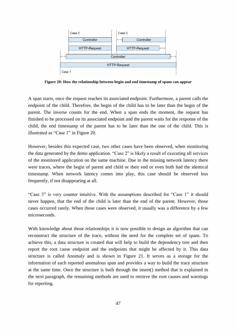
47
Figure 20: How the relationship between begin and end timestamp of spans can appear
A span starts, once the request reaches its associated endpoint. Furthermore, a parent calls the
endpoint of the child. Therefore, the begin of the child has to be later than the begin of the
parent. The inverse counts for the end. When a span ends the moment, the request has
finished to be processed on its associated endpoint and the parent waits for the response of the
child, the end timestamp of the parent has to be later than the one of the child. This is
illustrated as “Case 1” in Figure 20.
However, besides this expected case, two other cases have been observed, when monitoring
the data generated by the demo application. “Case 2” is likely a result of executing all services
of the monitored application on the same machine. Due to the missing network latency there
were traces, where the begin of parent and child or their end or even both had the identical
timestamp. When network latency comes into play, this case should be observed less
frequently, if not disappearing at all.
“Case 3” is very counter intuitive. With the assumptions described for “Case 1” it should
never happen, that the end of the child is later than the end of the parent. However, those
cases occurred rarely. When those cases were observed, it usually was a difference by a few
microseconds.
With knowledge about those relationships it is now possible to design an algorithm that can
reconstruct the structure of the trace, without the need for the complete set of spans. To
achieve this, a data structure is created that will help to build the dependency tree and then
report the root cause endpoint and the endpoints that might be affected by it. This data
structure is called Anomaly and is shown in Figure 21. It serves as a storage for the
information of each reported anomalous span and provides a way to build the trace structure
at the same time. Once the structure is built through the insert() method that is explained in
the next paragraph, the remaining methods are used to retrieve the root causes and warnings
for reporting.

48
Figure 21: UML class diagram of the root cause analysis data structure “Anomaly”
As the data structure is designed to rebuild the dependency structure of a trace, the prepared
anomalous spans have to be grouped by their trace IDs. Then they must be brought into the
order in which they originally started. This is done by sorting first by the begin timestamp and
then by the end timestamp. However, this step is the weak point of this algorithm when
looking at “Case 2” from Figure 20. In the case that the begin and end of two spans are
identical, the order of those two spans could be mixed up. However, as in some cases a http
request span and its corresponding span for processing in the controller class share the same
span ID, the span ID of the controller spans gets the ending “mvc” attached, when they are
reported from the anomaly detection algorithms. This means that in some of the cases the
spans can be brought into the right order reliably, even though their begin and end are
identical. Identifying a way to improve the sorting further would make the root cause analysis
more robust against this issue.
After sorting, the anomalous spans are converted into Anomaly objects. The Anomaly object
with the earliest beginning is the root and all the other Anomaly objects of the trace are
inserted into the root by calling its insert function. The Scala implementation of the insert
method is shown in Listing 3. It is a recursive function. The inserted anomaly is compared
against the children of the anomaly it is inserted into. If its parent ID matches the ID of a
child, or its begin and end are within the begin and end of one, it will be inserted into it. If
none of those conditions apply, it will be added to the list of children of the anomaly where it
was inserted into. In this way, the inserted anomaly will go further down the trace tree, until it
does either not match the insert conditions, or there are no anomalies left to insert it into. In
the last case, it will be a new leave in the tree of anomalies.

49
def insert(anomaly: Anomaly): Unit = { var inserted = false for (child <- children) { if (anomaly.parentId==this.spanId ||(anomaly.begin > child.begin && anomaly.end <= child.end) ||anomaly.begin >= child.begin && anomaly.end < child.end) { if (!inserted) { child.insert(anomaly) inserted = true} } } if (!inserted) { children.append(anomaly) anomaly.parent = this } }
Listing 3: Anomaly insert method (Scala)
Once the tree is created, the method getRootCauses will return a list of all anomaly objects
that are leave nodes in the anomaly tree. Those are the anomalies, where the associated
endpoints are most likely the root cause for the set of anomalies. By calling the getWarnings
method on each of those root causes, a list of all endpoints that lie on the path to the root of
the anomaly tree are returned. Those are the reported anomalous endpoints that are likely to
be the result of the anomaly propagation from the issue at the root cause endpoint. The
endpoint identifiers and error descriptors of the root causes are persisted in a database
together with the endpoint identifiers of their warnings. This information is then available for
the final visualization step.
5.2.3 Warning elimination
During the visualization, one more step is performed that enhances the result of the root cause
analysis. As the whole root cause analysis is based on mini batch processing that contains all
spans of a trace, it can happen that some of the spans are missing, as they slipped into another
mini batch. If those missing spans are containing the root causes, another endpoint identifier
will be written to the data base as the identified root cause, that would be just a warning, when
the trace would have been processed as a whole. Therefore, all anomalies are deprioritized to
a warning, if they appear in the set of warnings of another root cause. This means, they will
never be lost completely, just in case they happen to be a real anomaly – but they are assigned
a lower priority in the reporting. This enables the person in charge of chasing down the root
cause of an anomaly to start with the high priority anomalies and later transition to the lower
priority warnings, if still necessary.

50
After applying the steps of the root cause analysis and the warning elimination to the
anomalies that were reported from the different detection algorithms, a more differentiated
view on the problem is possible. In Figure 19, that represented the result after just the
anomaly detection stage, all the propagated anomalies were reported as anomalies. The
reporting after the root cause analysis and warning elimination looks different. As illustrated
in Figure 22, now the anomalies that were reported in services that rely on the anomalous
service E, are reported as warnings and only service E is reported as anomaly.
Figure 22: Differentiated reporting of anomalies (red circle) and warnings (yellow circle)
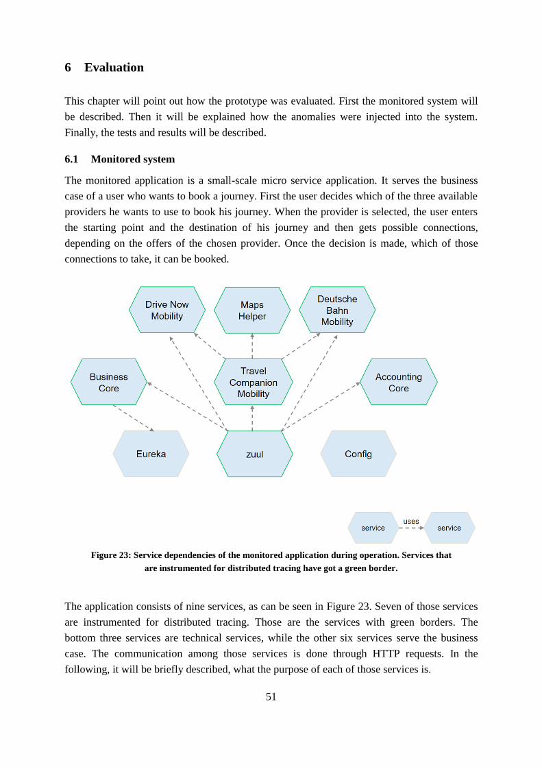
51
6 Evaluation
This chapter will point out how the prototype was evaluated. First the monitored system will
be described. Then it will be explained how the anomalies were injected into the system.
Finally, the tests and results will be described.
6.1 Monitored system
The monitored application is a small-scale micro service application. It serves the business
case of a user who wants to book a journey. First the user decides which of the three available
providers he wants to use to book his journey. When the provider is selected, the user enters
the starting point and the destination of his journey and then gets possible connections,
depending on the offers of the chosen provider. Once the decision is made, which of those
connections to take, it can be booked.
Figure 23: Service dependencies of the monitored application during operation. Services that
are instrumented for distributed tracing have got a green border.
The application consists of nine services, as can be seen in Figure 23. Seven of those services
are instrumented for distributed tracing. Those are the services with green borders. The
bottom three services are technical services, while the other six services serve the business
case. The communication among those services is done through HTTP requests. In the
following, it will be briefly described, what the purpose of each of those services is.
52
Starting with the technical services, the Eureka service is responsible for locating the
available services and making this information available to the other services in the
application. It offers the possibility to other services, to query, which services are currently
available in the micro service application.
The configuration service is a central instance, that is holding all the configuration
information for each service. At startup, each service retrieves its configuration from this
service. This enables a centralized configuration management.
The last of the three technical services, and the only one that is instrumented with distributed
tracing, is the zuul service. It is responsible for routing of requests and for authentication. In
the case of this application, the requests will all be made to the port zuul is running on. Zuul
then takes care to forward the requests to the proper port for the requested service.
Additionally, during this process it makes sure, the user that is requesting the service is
authenticated and authorized.
The first service a user interacts with, when booking a journey, is the Business Core service.
It queries the Eureka service for the currently available mobility services and provides a list of
links to the user, who can choose, which of the mobility services to use. Only the services that
are currently up and running will be presented to the user.
The three mobility services all work similar. They accept a starting point and a destination
and then provide a set of possible connections to the user. The Deutsche Bahn Mobility
service and the Drive Now Mobility service both pull the requests directly from a database.
However, the Travel Companion Mobility service requests the possible connections from both
the other mobility services and furthermore adds some distance information based on
calculations of the Maps Helper service. Therefore, the request to the Travel Companion
Mobility service is the most complex request in terms of involved services.
The last service of this micro services application is the Accounting Core service. It is
responsible of writing the booked connection of the user to the database.
6.2 Evaluation Setup
To evaluate the ability of the prototype to detect the anomalies defined in section 4.2, first the
monitored application is instrumented to enable the injection of those types of anomalies and
a training set is generated. This is the preparation before the tests to evaluate the prototype
can be performed.

53
As instrumenting the application for anomaly injection is a manual task, the evaluation will be
restricted to a single request that will be executed repeatedly. As in the previous chapter
described, the request to the Travel Companion Mobility service includes the most calls to
other services – exactly what is useful for this evaluation. The involved services can be seen
in Figure 24. The path of the request is shown in red. It enters the system through a request to
the zuul service. To serve the request the Travel Companion Mobility Service, the Drive Now
Mobility service, the Deutsche Bahn Mobility service and the Maps Helper service are
involved. The high number of involved services is the reason why this request will be selected
for the evaluation.
Figure 24: Flow of the monitored request (red arrows)
6.2.1 Anomaly Injections
The information, whether an anomaly should be injected into a request or not, should be
added on the request level. This means, depending on parameters in the request, the anomaly
should appear or not. To achieve this, for all requests (see Figure 24), a new parameter will be
added. This parameter is a string that carries the information whether an anomaly should be
triggered and if yes, where and which kind.
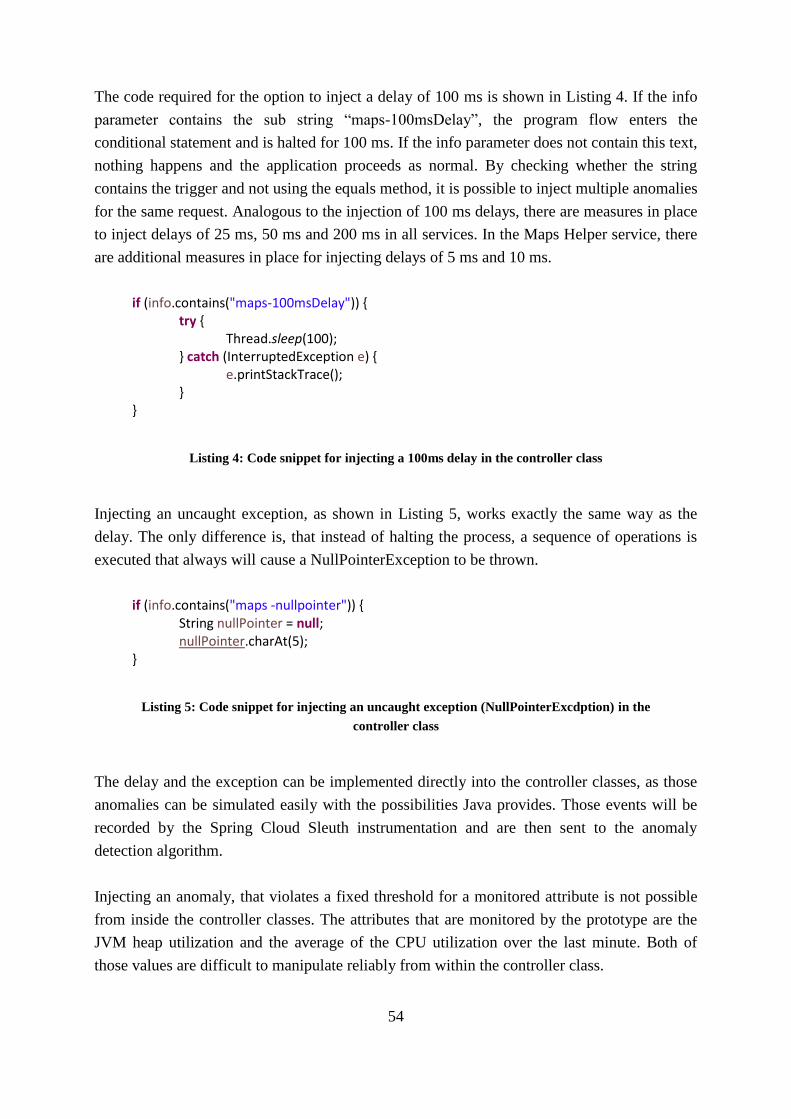
54
The code required for the option to inject a delay of 100 ms is shown in Listing 4. If the info
parameter contains the sub string “maps-100msDelay”, the program flow enters the
conditional statement and is halted for 100 ms. If the info parameter does not contain this text,
nothing happens and the application proceeds as normal. By checking whether the string
contains the trigger and not using the equals method, it is possible to inject multiple anomalies
for the same request. Analogous to the injection of 100 ms delays, there are measures in place
to inject delays of 25 ms, 50 ms and 200 ms in all services. In the Maps Helper service, there
are additional measures in place for injecting delays of 5 ms and 10 ms.
if (info.contains("maps-100msDelay")) { try { Thread.sleep(100); } catch (InterruptedException e) { e.printStackTrace(); } }
Listing 4: Code snippet for injecting a 100ms delay in the controller class
Injecting an uncaught exception, as shown in Listing 5, works exactly the same way as the
delay. The only difference is, that instead of halting the process, a sequence of operations is
executed that always will cause a NullPointerException to be thrown.
if (info.contains("maps -nullpointer")) { String nullPointer = null; nullPointer.charAt(5); }
Listing 5: Code snippet for injecting an uncaught exception (NullPointerExcdption) in the
controller class
The delay and the exception can be implemented directly into the controller classes, as those
anomalies can be simulated easily with the possibilities Java provides. Those events will be
recorded by the Spring Cloud Sleuth instrumentation and are then sent to the anomaly
detection algorithm.
Injecting an anomaly, that violates a fixed threshold for a monitored attribute is not possible
from inside the controller classes. The attributes that are monitored by the prototype are the
JVM heap utilization and the average of the CPU utilization over the last minute. Both of
those values are difficult to manipulate reliably from within the controller class.

55
However, there is another location where the anomaly can be injected reliably. This is inside
the distributed tracing extension, that was implemented to add information about heap
utilization and CPU utilization to the reported spans. In this place, the code snippet shown in
Listing 6 is inserted. By reading information from the HTTP request, it is possible to identify
the URI of the request that is currently processed. Furthermore, as the tracer, that is taking
care of creating the spans of the distributed tracing instrumentation, is available at this
location in the application, the parameter with the info about the anomaly injection can be
accessed.
String requestUri = httpRequest.getRequestURI(); String infoParam = tracer.getCurrentSpan().tags().getOrDefault("servlet.param.info", "not set"); if (infoParam.contains("maps-highCPU") && requestUri.equals("/maps-helper-service/distance")) { tracer.addTag("cpu.system.utilizationAvgLastMinute", "99"); }
Listing 6: Code snippet to inject a high CPU utilization value inside the distributed tracing
extension
If the info parameter contains the required string and the URI does match, the CPU utilization
tag will be overwritten with a value of 99. As the anomaly detection algorithm will only read
the value, this is sufficient to inject an anomaly that will trigger the violation of a fixed
threshold on the CPU utilization without the need to really impact the CPU.
6.2.2 Test set generation
To train the Splitted KMeans algorithm for the detection of increased response times, a set of
historical data has to be available. To create this set, a large number of requests has to be sent
to the application and recorded by the Spring Cloud Sleuth instrumentation. The recorded data
will be stored in a Kafka topic and is then available for training the Splitted KMeans
algorithm, when the anomaly detection is started.
To have a consistent way of sending the requests throughout the whole evaluation, JMeter
[85] will be used to send the requests. JMeter is a software that is designed for performance
testing of applications. There are different possibilities to configure a request and send it
repeatedly. Furthermore, there are ways to record the results of the sent requests.
To generate the training set, JMeter is set up to run requests against the Travel Companion
Mobility Service through the zuul service. This will result in the request flow that was
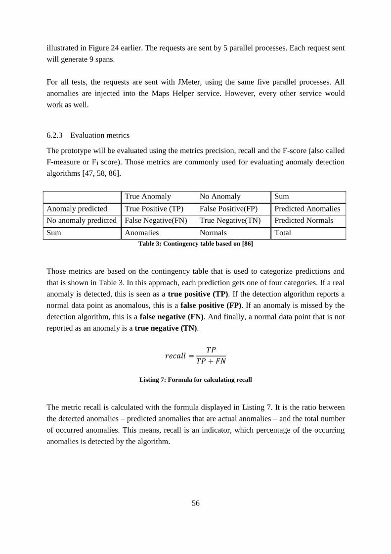
56
illustrated in Figure 24 earlier. The requests are sent by 5 parallel processes. Each request sent
will generate 9 spans.
For all tests, the requests are sent with JMeter, using the same five parallel processes. All
anomalies are injected into the Maps Helper service. However, every other service would
work as well.
6.2.3 Evaluation metrics
The prototype will be evaluated using the metrics precision, recall and the F-score (also called
F-measure or F1 score). Those metrics are commonly used for evaluating anomaly detection
algorithms [47, 58, 86].
True Anomaly No Anomaly Sum
Anomaly predicted True Positive (TP) False Positive(FP) Predicted Anomalies
No anomaly predicted False Negative(FN) True Negative(TN) Predicted Normals
Sum Anomalies Normals Total
Table 3: Contingency table based on [86]
Those metrics are based on the contingency table that is used to categorize predictions and
that is shown in Table 3. In this approach, each prediction gets one of four categories. If a real
anomaly is detected, this is seen as a true positive (TP). If the detection algorithm reports a
normal data point as anomalous, this is a false positive (FP). If an anomaly is missed by the
detection algorithm, this is a false negative (FN). And finally, a normal data point that is not
reported as an anomaly is a true negative (TN).
𝑟𝑒𝑐𝑎𝑙𝑙 =𝑇𝑃
𝑇𝑃 + 𝐹𝑁
Listing 7: Formula for calculating recall
The metric recall is calculated with the formula displayed in Listing 7. It is the ratio between
the detected anomalies – predicted anomalies that are actual anomalies – and the total number
of occurred anomalies. This means, recall is an indicator, which percentage of the occurring
anomalies is detected by the algorithm.

57
𝑝𝑟𝑒𝑐𝑖𝑠𝑖𝑜𝑛 =𝑇𝑃
𝑇𝑃 + 𝐹𝑃
Listing 8: Formula for calculating precision
The metric precision is calculated with the formula displayed in Listing 8. It is the ratio
between the detected anomalies and the number of reported anomalies. This metric is an
indicator for how reliable a data point that is reported as an anomaly by the algorithm is really
an anomaly.
𝐹-𝑠𝑐𝑜𝑟e =2 ∙ 𝑝𝑟𝑒𝑐𝑖𝑠𝑖𝑜𝑛 ∙ 𝑟𝑒𝑐𝑎𝑙𝑙
𝑝𝑟𝑒𝑐𝑖𝑠𝑖𝑜𝑛 + 𝑟𝑒𝑐𝑎𝑙𝑙
Listing 9: Formula for calculating the F-score based on precision and recall
To improve precision, the false positives have to be reduced. On the other hand, to improve
recall, the false negatives have to be reduced. As usually the improvement of one of those
metrics results in a worse result for the other, the F-Score was introduced as a quality measure
that takes the harmonic mean of precision and recall. For equal weights on precision and
recall, as it will be used for the evaluation, the formula is shown in Listing 9. This metric goes
back on a suggestion of van Rijsbergen [87].
6.2.4 Measurement points
To get the most information out of the test, the required metrics are calculated on three
different stages of the prototype for each test. First the results that come out from the anomaly
detection stage are observed. This means, the raw performance of the anomaly detection
algorithms in this setting can be evaluated, before any enhancing processing is performed on
the detected anomalies. This stage is called “anomaly detection” in the result tables.
Then the results after applying the basic root cause analysis are evaluated. This gives an
insight how the root cause analysis works and what the calculated context is able to give as
improvement to the process of detecting meaningful anomalies. This stage is called “root
cause analysis” in the result tables.
And finally, the results after removing anomalies that have been reported as warnings before,
is analyzed. This step is removing the mistakenly reported anomalies, that resulted from a
trace being processed over more than one mini batch. This stage is called “warning
elimination” in the result tables.
58
6.3 Prototype Evaluation
In a first set of tests, the whole prototype is evaluated for its capabilities to detect errors,
increased response times and violations of a fixed threshold. This is tested by running the
algorithms in parallel. The focus of this set of tests is on the behavior of the system as a
whole. The training set contains 20,000 requests.
6.3.1 Performed tests
To evaluate the capability of the prototype to detect the anomalies defined in chapter 4.2, five
tests are performed. Before running the test, all three algorithms, described in chapters 4.4.4,
4.4.5 and 4.4.6, are started to run in parallel.
For the first test, 500 requests without any injected anomalies are sent to the monitored
application. This test tries to figure out, how many false positives will be issued by the
application, when no anomalies are present.
The next two tests are targeted towards the capability of detecting increased response times.
For the second test, delays of 100 milliseconds are injected and a total number of 100 requests
is sent. The third test is similar to the second one, with the difference, that the injected delays
are only lasting for 50 milliseconds. The normal duration of the request, the delays were
injected into was about 7ms.
The fourth test is about detecting uncaught exceptions. To evaluate the performance of the
error detection algorithm, 100 requests are sent with injected NullPointerExceptions.
And finally, the fifth test targets the capabilities of detecting the violation of fixed thresholds.
The fixed threshold detector is set up to monitor the CPU utilization average over the last
minute and raise an alarm if the value gets above 98%. To test the detector, 100 requests are
sent with an injected CPU utilization average of 99%:
During all tests, the complete set of detectors was running. This means, that at any stage of
the evaluation all sensors could potentially detect an anomaly. So, even though all the tests
are targeted at specific detectors, it can happen, that another detector will report false
positives.
6.3.2 Results
Each request generates nine spans, which are examined by the anomaly detection algorithms,
whether they are anomalous or normal. In case an anomaly is injected, exactly one of those
nine spans is anomalous per request. The other spans are normal.
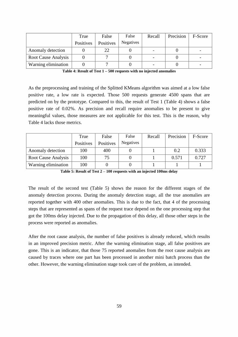
59
True
Positives
False
Positives
False
Negatives
Recall Precision F-Score
Anomaly detection 0 22 0 - 0 -
Root Cause Analysis 0 7 0 - 0 -
Warning elimination 0 7 0 - 0 -
Table 4: Result of Test 1 – 500 requests with no injected anomalies
As the preprocessing and training of the Splitted KMeans algorithm was aimed at a low false
positive rate, a low rate is expected. Those 500 requests generate 4500 spans that are
predicted on by the prototype. Compared to this, the result of Test 1 (Table 4) shows a false
positive rate of 0.02%. As precision and recall require anomalies to be present to give
meaningful values, those measures are not applicable for this test. This is the reason, why
Table 4 lacks those metrics.
True
Positives
False
Positives
False
Negatives
Recall Precision F-Score
Anomaly detection 100 400 0 1 0.2 0.333
Root Cause Analysis 100 75 0 1 0.571 0.727
Warning elimination 100 0 0 1 1 1
Table 5: Result of Test 2 – 100 requests with an injected 100ms delay
The result of the second test (Table 5) shows the reason for the different stages of the
anomaly detection process. During the anomaly detection stage, all the true anomalies are
reported together with 400 other anomalies. This is due to the fact, that 4 of the processing
steps that are represented as spans of the request trace depend on the one processing step that
got the 100ms delay injected. Due to the propagation of this delay, all those other steps in the
process were reported as anomalies.
After the root cause analysis, the number of false positives is already reduced, which results
in an improved precision metric. After the warning elimination stage, all false positives are
gone. This is an indicator, that those 75 reported anomalies from the root cause analysis are
caused by traces where one part has been processed in another mini batch process than the
other. However, the warning elimination stage took care of the problem, as intended.

60
True
Positives
False
Positives
False
Negatives
Recall Precision F-Score
Anomaly detection 100 110 0 1 0.476 0.645
Root Cause Analysis 95 9 5 0.95 0.913 0.931
Warning elimination 95 3 5 0.95 0.969 0.960
Table 6: Result of Test 3 – 100 requests with an injected 50ms delay
The result of Test 3 (Table 6) shows issues, the prototype can run into. While the anomaly
detection is able to identify all of the injected anomalies, five of those are lost after the root
cause analysis was performed. This is due to the fact, that the root cause analysis relies on
sorting the anomalous spans into the order in which they appeared, before processing them. In
the case begin and end are identical, it can happen that the order is mixed up and therefore the
wrong anomalies are reported.
As those wrong predictions will be eliminated in the warning elimination, the remaining false
positives are due to false positive predictions in services that do not depend on the anomalous
service. This issue can only be addressed by increasing the threshold of the Splitted KMeans
predictor.
True
Positives
False
Positives
False
Negatives
Recall Precision F-Score
Anomaly detection 100 178 0 1 0.360 0.529
Root Cause Analysis 100 34 0 1 0.746 0.855
Warning elimination 100 15 0 1 0.870 0.930
Table 7: Result of Test 4 – 100 requests with injected NullPointerException
Test 4 (Table 7) shows that all of the injected exceptions are detected. The propagated errors
are eliminated by the root cause analysis. The remaining false positives are false reports by
the Splitted KMeans algorithm.
True
Positives
False
Positives
False
Negatives
Recall Precision F-Score
Anomaly detection 100 0 0 1 1 1
Root Cause Analysis 100 0 0 1 1 1
Warning elimination 100 0 0 1 1 1
Table 8: Result of Test 5 – 100 requests with a high CPU utilization value injected
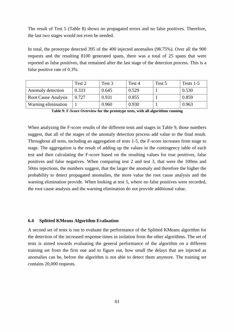
61
The result of Test 5 (Table 8) shows no propagated errors and no false positives. Therefore,
the last two stages would not even be needed.
In total, the prototype detected 395 of the 400 injected anomalies (98.75%). Over all the 900
requests and the resulting 8100 generated spans, there was a total of 25 spans that were
reported as false positives, that remained after the last stage of the detection process. This is a
false positive rate of 0.3%.
Test 2 Test 3 Test 4 Test 5 Tests 1-5
Anomaly detection 0.333 0.645 0.529 1 0.530
Root Cause Analysis 0.727 0.931 0.855 1 0.859
Warning elimination 1 0.960 0.930 1 0.963
Table 9: F-Score Overview for the prototype tests, with all algorithms running
When analyzing the F-score results of the different tests and stages in Table 9, those numbers
suggest, that all of the stages of the anomaly detection process add value to the final result.
Throughout all tests, including an aggregation of tests 1-5, the F-score increases from stage to
stage. The aggregation is the result of adding up the values in the contingency table of each
test and then calculating the F-score based on the resulting values for true positives, false
positives and false negatives. When comparing test 2 and test 3, that were the 100ms and
50ms injections, the numbers suggest, that the larger the anomaly and therefore the higher the
probability to detect propagated anomalies, the more value the root cause analysis and the
warning elimination provide. When looking at test 5, where no false positives were recorded,
the root cause analysis and the warning elimination do not provide additional value.
6.4 Splitted KMeans Algorithm Evaluation
A second set of tests is run to evaluate the performance of the Splitted KMeans algorithm for
the detection of the increased response times in isolation from the other algorithms. The set of
tests is aimed towards evaluating the general performance of the algorithm on a different
training set from the first one and to figure out, how small the delays that are injected as
anomalies can be, before the algorithm is not able to detect them anymore. The training set
contains 20,000 requests.
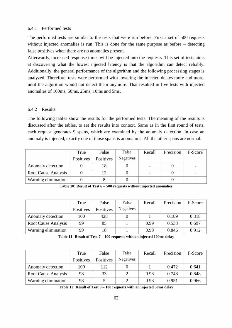
62
6.4.1 Performed tests
The performed tests are similar to the tests that were run before. First a set of 500 requests
without injected anomalies is run. This is done for the same purpose as before – detecting
false positives when there are no anomalies present.
Afterwards, increased response times will be injected into the requests. This set of tests aims
at discovering what the lowest injected latency is that the algorithm can detect reliably.
Additionally, the general performance of the algorithm and the following processing stages is
analyzed. Therefore, tests were performed with lowering the injected delays more and more,
until the algorithm would not detect them anymore. That resulted in five tests with injected
anomalies of 100ms, 50ms, 25ms, 10ms and 5ms.
6.4.2 Results
The following tables show the results for the performed tests. The meaning of the results is
discussed after the tables, to set the results into context. Same as in the first round of tests,
each request generates 9 spans, which are examined by the anomaly detection. In case an
anomaly is injected, exactly one of those spans is anomalous. All the other spans are normal.
True
Positives
False
Positives
False
Negatives
Recall Precision F-Score
Anomaly detection 0 18 0 - 0 -
Root Cause Analysis 0 12 0 - 0 -
Warning elimination 0 8 0 - 0 -
Table 10: Result of Test 6 – 500 requests without injected anomalies
True
Positives
False
Positives
False
Negatives
Recall Precision F-Score
Anomaly detection 100 428 0 1 0.189 0.318
Root Cause Analysis 99 85 1 0.99 0.538 0.697
Warning elimination 99 18 1 0.99 0.846 0.912
Table 11: Result of Test 7 – 100 requests with an injected 100ms delay
True
Positives
False
Positives
False
Negatives
Recall Precision F-Score
Anomaly detection 100 112 0 1 0.472 0.641
Root Cause Analysis 98 33 2 0.98 0.748 0.848
Warning elimination 98 5 2 0.98 0.951 0.966
Table 12: Result of Test 8 – 100 requests with an injected 50ms delay
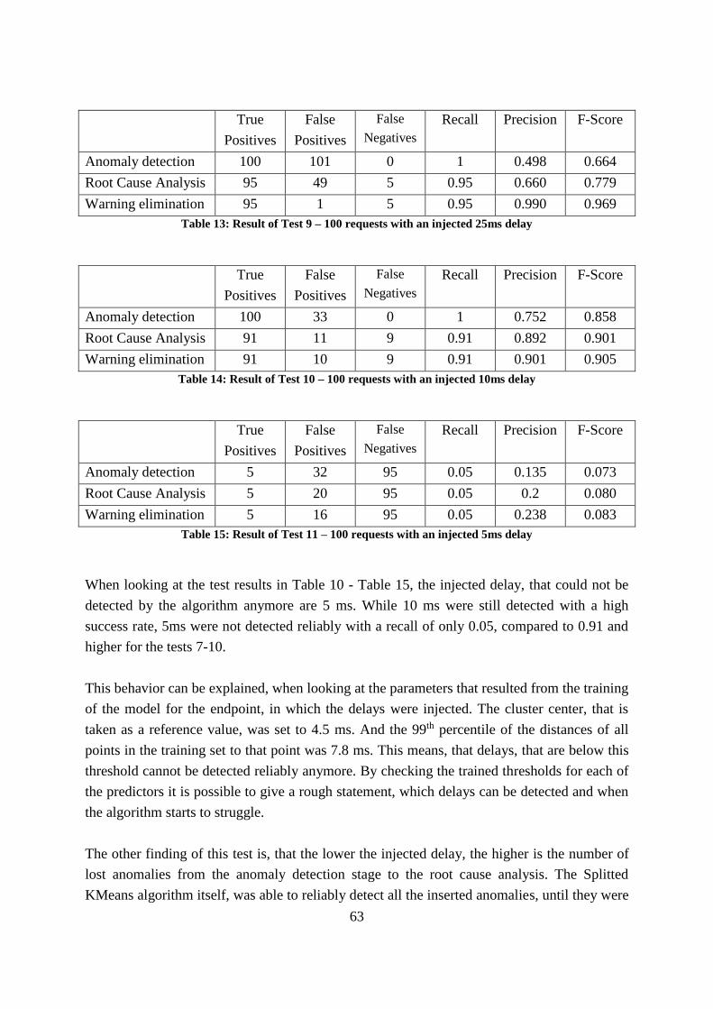
63
True
Positives
False
Positives
False
Negatives
Recall Precision F-Score
Anomaly detection 100 101 0 1 0.498 0.664
Root Cause Analysis 95 49 5 0.95 0.660 0.779
Warning elimination 95 1 5 0.95 0.990 0.969
Table 13: Result of Test 9 – 100 requests with an injected 25ms delay
True
Positives
False
Positives
False
Negatives
Recall Precision F-Score
Anomaly detection 100 33 0 1 0.752 0.858
Root Cause Analysis 91 11 9 0.91 0.892 0.901
Warning elimination 91 10 9 0.91 0.901 0.905
Table 14: Result of Test 10 – 100 requests with an injected 10ms delay
True
Positives
False
Positives
False
Negatives
Recall Precision F-Score
Anomaly detection 5 32 95 0.05 0.135 0.073
Root Cause Analysis 5 20 95 0.05 0.2 0.080
Warning elimination 5 16 95 0.05 0.238 0.083
Table 15: Result of Test 11 – 100 requests with an injected 5ms delay
When looking at the test results in Table 10 - Table 15, the injected delay, that could not be
detected by the algorithm anymore are 5 ms. While 10 ms were still detected with a high
success rate, 5ms were not detected reliably with a recall of only 0.05, compared to 0.91 and
higher for the tests 7-10.
This behavior can be explained, when looking at the parameters that resulted from the training
of the model for the endpoint, in which the delays were injected. The cluster center, that is
taken as a reference value, was set to 4.5 ms. And the 99th percentile of the distances of all
points in the training set to that point was 7.8 ms. This means, that delays, that are below this
threshold cannot be detected reliably anymore. By checking the trained thresholds for each of
the predictors it is possible to give a rough statement, which delays can be detected and when
the algorithm starts to struggle.
The other finding of this test is, that the lower the injected delay, the higher is the number of
lost anomalies from the anomaly detection stage to the root cause analysis. The Splitted
KMeans algorithm itself, was able to reliably detect all the inserted anomalies, until they were
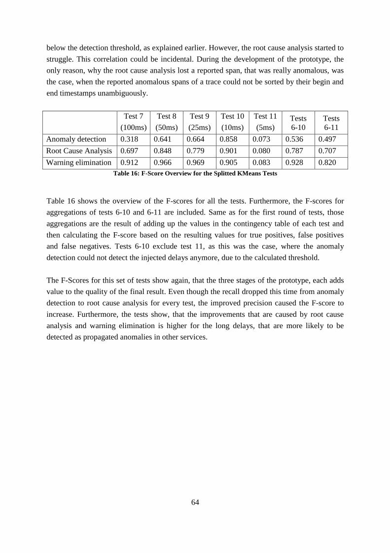
64
below the detection threshold, as explained earlier. However, the root cause analysis started to
struggle. This correlation could be incidental. During the development of the prototype, the
only reason, why the root cause analysis lost a reported span, that was really anomalous, was
the case, when the reported anomalous spans of a trace could not be sorted by their begin and
end timestamps unambiguously.
Test 7
(100ms)
Test 8
(50ms)
Test 9
(25ms)
Test 10
(10ms)
Test 11
(5ms)
Tests
6-10
Tests
6-11
Anomaly detection 0.318 0.641 0.664 0.858 0.073 0.536 0.497
Root Cause Analysis 0.697 0.848 0.779 0.901 0.080 0.787 0.707
Warning elimination 0.912 0.966 0.969 0.905 0.083 0.928 0.820
Table 16: F-Score Overview for the Splitted KMeans Tests
Table 16 shows the overview of the F-scores for all the tests. Furthermore, the F-scores for
aggregations of tests 6-10 and 6-11 are included. Same as for the first round of tests, those
aggregations are the result of adding up the values in the contingency table of each test and
then calculating the F-score based on the resulting values for true positives, false positives
and false negatives. Tests 6-10 exclude test 11, as this was the case, where the anomaly
detection could not detect the injected delays anymore, due to the calculated threshold.
The F-Scores for this set of tests show again, that the three stages of the prototype, each adds
value to the quality of the final result. Even though the recall dropped this time from anomaly
detection to root cause analysis for every test, the improved precision caused the F-score to
increase. Furthermore, the tests show, that the improvements that are caused by root cause
analysis and warning elimination is higher for the long delays, that are more likely to be
detected as propagated anomalies in other services.

65
7 Conclusion
The final chapter of this thesis will wrap things up. Findings and limitations will be pointed
out and perspectives for future work will be suggested.
7.1 Findings
The first finding of the thesis is, that it is possible to detect anomalies by just using
information from distributed tracing. The three implemented algorithms were able to detect
all the anomalies that were targeted, namely error, fixed threshold violations and increased
response time compared to the normal behavior of a service.
The evaluation of the prototype (see Chapter 6), with all algorithms running in parallel,
showed that the algorithms work together effectively. Besides the high detection rate of the
injected anomalies of 98.75%, the false positive rate, when no anomalies were injected was at
0.2%. The separate evaluation of the Splitted KMeans algorithms that is used to detect
performance anomalies, showed that the algorithm detects anomalies reliably until the delay
gets lower than the calculated threshold. By examining the thresholds, that result for each
endpoint after the training phase, assumptions can be made, which delays will be detected and
which will be missed.
Furthermore, the prototype is capable of recreating the dependency context from a set of
spans that have been reported as anomalous, in all cases where the anomalous spans can be
brought into the order in which they were created by the attached timestamps. It is not
necessary that the whole trace with all spans and an unbroken chain of parent and child
relationships is present. Information that is available from distributed tracing is enough for the
task. This is useful in suggesting the endpoint, the anomalous span that is furthest down the
call hierarchy to be the most likely root cause for the set of anomalies.
The whole prototype is designed in a way, that it can be changed easily in the future. The
distributed tracing instrumentation, the anomaly detection and the root cause analysis are
connected through asynchronous messaging. This means, as long as the messaging formats
are not changed, each of those modules can be replaced. Furthermore, the prototype is
designed, so that multiple anomaly detection algorithms can be run in parallel. This means,
that in the case a new type of anomalies should be detected, a new algorithm can be written
and then plugged in besides the already available algorithms. Or if an existing algorithm is not
performing as intended, it can be removed without impacting the other algorithms running in
parallel.

66
Finally, the whole prototype is built on open source frameworks with scalability in mind.
Especially Apache Spark and Apache Kafka are able to run in cluster mode. This means, the
processing power of the system can be increased by running the application on a cluster to
meet the need of processing more data in a production scenario with a larger number of
services and endpoints.
7.2 Limitations
Besides all the positive results of this thesis, the work has its limitations. Those will be
described in the following.
The first limitation that came up during the extension of the tracing instrumentation, was the
fact, that system level metrics are hard to fetch from inside of Java applications. With relying
on APIs of the JVM to access system level metrics, the amount of metrics that is available is
limited by those. Furthermore, it can be very expensive to gather this information. When
adding CPU metrics to the tracing information, the first approach was to take the current
utilization. This required a continuous processing effort by the instrumentation extension. The
CPU utilization average over the last minute, that is provided by the JVM, is not as precise,
but does not need the ongoing processing. Therefore, it was used for the instrumentation
instead, to keep the impact on the instrumented application as low as possible.
The next limitation of this work is about the root cause analysis. The root cause analysis as it
is implemented does only work, if anomalies are reported as outliers – this means as
anomalous spans. This has the consequence, that all algorithms that only work by detecting
anomalous time series instead of outliers, are not working in this prototype.
Furthermore, the root cause analysis, that is only using distributed tracing information, is
performed in the context of a trace and the anomalous spans that have been reported for it by
the anomaly detection algorithms. This is the context this algorithm has available. There is no
other reference data, which the results can be compared against, or where results that might
appear off, could be corrected with. This is especially relevant, as the algorithm for creating
the dependency context among the reported anomalous spans, relies on bringing those spans
into the order they were started. However, in some rare cases this order is ambiguous what
results in impacting the reported anomalies and warnings.
Another limitation of the current approach are asynchronous requests. Especially “fire and
forget” requests, like writing to a database without waiting for a confirmation, is currently not
covered by the implementation of the root cause analysis.
The last limitation concerns the scope of the evaluation of the prototype. The evaluation was
performed against a demo application that ran on the same local machine with all the services.

67
In a production environment, the services would run on different machines and the number of
requests and endpoints to monitor would be much larger. As no data from production or a
production application to monitor was available, the system could not be tested in large scale.
7.3 Suggestions for future work
The first suggestions for future work is to improve the evaluation of the system. Getting
access to a data set from a production environment, or even instrumenting a microservice
application that is running in production would give a lot of insight into the capabilities of the
prototype. By now, the scaling capability has not been verified – the application was designed
on frameworks, that allow for running them on a cluster for scaling – however, there is no
proof yet.
The next suggestion would be the improvement of the root cause analysis. By relaxing the
requirement to getting all information from the spans at hand, it could be possible to include
externally calculated information on the service and endpoint dependencies into the
algorithm. This would have three big advantages. First this would be a reliable source of
information, that will know the dependencies for sure – even if some information inside a
trace gets mixed up or behaves unexpectedly. Second, it would make it easier to handle
asynchronous requests properly. The third advantage is, that the availability of the
dependencies would enable the prototype to use algorithms that do predict on time series data,
as no trace context would be needed anymore and it would be sufficient to identify the
endpoint that is behaving anomalous. This could be achieved by integrating this prototype,
with another prototype from this research group that is targeted at discovering microservice
structures and dependencies based on distributed tracing.
Another topic where further work could be focused to is the tracing instrumentation. This
thesis only touched briefly on the topic of including further metrics into the reported spans.
By analyzing thoroughly, which metrics could be obtained during the tracing process and how
much resources would be needed to get them, would benefit the anomaly detection with
providing a greater number of features to choose from. Furthermore, it would be interesting to
see how applications that cannot be instrumented with Spring Cloud Sleuth – as they are e.g.
no Java applications – can be instrumented, to provide a matching messaging format to be
included into the anomaly detection and root cause analysis process.
Finally, the last suggestion regards the visualization of the results. The visualization that is
provided by this prototype does only work for the request that was used in the evaluation
phase. A proper visualization would have to deal with displaying a large amount of services,

68
as microservice applications can get very complex. Furthermore, it would need to display the
reported anomalies in a way that is easy to understand by the operator and provides as much
information as is necessary. As other work in this research group focuses at exactly this topic,
an integration with this project would be very beneficial.

69
References
[1] J. Bogner and A. Zimmermann, “Towards Integrating Microservices with Adaptable
Enterprise Architecture,” in 2016 IEEE 20th International Enterprise Distributed Object
Computing Workshop (EDOCW), Vienna, Austria, 2016, pp. 1–6.
[2] M. Kim, R. Sumbaly, and S. Shah, “Root cause detection in a service-oriented
architecture,” ACM SIGMETRICS Performance Evaluation Review, vol. 41, no. 1, pp.
93–104, 2013.
[3] J. Mukherjee, M. Wang, and D. Krishnamurthy, “Performance Testing Web Applications
on the Cloud,” in 2014 IEEE Seventh International Conference on Software Testing,
Verification and Validation Workshops, OH, USA, 2014, pp. 363–369.
[4] G. Linden, Marissa Mayer at Web 2.0. [Online] Available:
http://glinden.blogspot.de/2006/11/marissa-mayer-at-web-20.html. Accessed on:
05.05.2017.
[5] N. Shalom, Amazon found every 100ms of latency cost them 1% in sales. | GigaSpaces
Blog. [Online] Available: http://blog.gigaspaces.com/amazon-found-every-100ms-of-
latency-cost-them-1-in-sales/. Accessed on: 05.05.2017.
[6] Walmart, Walmart pagespeed-slide. [Online] Available:
https://de.slideshare.net/devonauerswald/walmart-pagespeedslide. Accessed on:
29.08.17.
[7] A. Almossawi, Firefox & Page Load Speed – Part I | Blog of Metrics. [Online]
Available: https://blog.mozilla.org/metrics/2010/03/31/firefox-page-load-speed-part-i/.
Accessed on: 05.05.2017.
[8] B. H. Sigelman et al., Dapper, a Large-Scale Distributed Systems Tracing Infrastructure.
[Online] Available:
https://static.googleusercontent.com/media/research.google.com/de//pubs/archive/36356.
pdf. Accessed on: 31.03.2017.
[9] C. Aniszczyk, Distributed Systems Tracing with Zipkin. [Online] Available:
https://blog.twitter.com/engineering/en_us/a/2012/distributed-systems-tracing-with-
zipkin.html. Accessed on: 27.08.17.
[10] Yelp, Distributed tracing at Yelp. [Online] Available:
https://engineeringblog.yelp.com/2016/04/distributed-tracing-at-yelp.html. Accessed on:
25.08.17.
[11] Pinterest, Distributed tracing at Pinterest with new open source tools. [Online]
Available: https://medium.com/@Pinterest_Engineering/distributed-tracing-at-pinterest-
with-new-open-source-tools-a4f8a5562f6b. Accessed on: 25.08.17.
[12] Uber, uber/jaeger. [Online] Available: https://github.com/uber/jaeger. Accessed on:
25.08.17.
[13] Y. Shkuro, Evolving Distributed Tracing at Uber Engineering. [Online] Available:
https://eng.uber.com/distributed-tracing/. Accessed on: 25.08.17.

70
[14] M. Fowler and J. Lewis, Microservices. [Online] Available:
https://martinfowler.com/articles/microservices.html. Accessed on: 02.05.2017.
[15] N. Dragoni et al., “Microservices - Yesterday, today, and tomorrow,” Accessed on:
02.05.2017.
[16] M. P. Papazoglou and W.-J. van den Heuvel, “Service oriented architectures:
Approaches, technologies and research issues,” The VLDB Journal, vol. 16, no. 3, pp.
389–415, 2007.
[17] R. Heinrich et al., “Performance Engineering for Microservices: Research Challenges
and Directions,” in Proceedings of the 8th ACM/SPEC on International Conference on
Performance Engineering Companion - ICPE '17 Companion, L'Aquila, Italy, 2017, pp.
223–226.
[18] S. Alpers, C. Becker, A. Oberweis, and T. Schuster, “Microservice Based Tool Support
for Business Process Modelling,” in 19th IEEE International Enterprise Distributed
Object Computing Conference workshops, EDOCW 2015, Adelaide, Australia, 2015, pp.
71–78.
[19] J. Thönes, “Microservices,” IEEE Softw., vol. 32, no. 1, p. 116, 2015.
[20] T. Mauro, Microservices at Netflix: Lessons for Architectural Design: based on a talk by
Adrian Cockroft. [Online] Available: https://www.nginx.com/blog/microservices-at-
netflix-architectural-best-practices/. Accessed on: 16.07.17.
[21] T. Stuart, Microservices and the monolith. [Online] Available:
https://developers.soundcloud.com/blog/microservices-and-the-monolith. Accessed on:
16.07.17.
[22] OpenZipkin - A distributed tracing system. [Online] Available: http://zipkin.io/. Accessed
on: 31.03.2017.
[23] M. Y. Chen, E. Kiciman, E. Fratkin, A. Fox, and E. Brewer, “Pinpoint: problem
determination in large, dynamic Internet services,” in Proceedings / International
Conference on Dependable Systems and Networks, Washington, DC, USA, 2002, pp.
595–604.
[24] P. Barham, R. Isaacs, R. Mortier, and D. Narayanan, “Magpie: online modelling and
performance-aware systems,” in Proceedings of HotOS IX: The 9th Workshop on Hot
Topics in Operating Systems, 2003, pp. 85–90.
[25] R. Fonseca, G. Porter, R. H. Katz, S. Shenker, and I. Stoica, “X-Trace: A Pervasive
Network Tracing Framework,” in Proceedings of the 4th USENIX conference on
Networked systems design & implementation, 2007.
[26] D. M. Hawkins, Identification of Outliers. Dordrecht: Springer, 1980.
71
[27] A. Bovenzi, F. Brancati, S. Russo, and A. Bondavalli, “A Statistical Anomaly-Based
Algorithm for On-line Fault Detection in Complex Software Critical Systems,” in
Lecture Notes in Computer Science, vol. 6894, Computer safety, reliability, and security:
30th international conference, SAFECOMP 2011, Naples, Italy, September 19 - 22,
2011, F. Flammini, S. Bologna, and V. Vittorini, Eds., Berlin: Springer, 2011, pp. 128–
142.
[28] N. Laptev, S. Amizadeh, and I. Flint, “Generic and Scalable Framework for Automated
Time-series Anomaly Detection,” in Proceedings of the 21st ACM SIGKDD
International Conference on Knowledge Discovery and Data Mining, August 10 - 13,
2015, Sydney, NSW, Australia, 2015, pp. 1939–1947.
[29] V. Chandola, A. Banerjee, and V. Kumar, “Anomaly detection: A survey,” ACM
Comput. Surv., vol. 41, no. 3, pp. 1–58, 2009.
[30] M. Gupta, A. Singh, H. Chen, and G. Jiang, “Context-Aware Time Series Anomaly
Detection for Complex Systems,” in Proc. of the SDM Workshop on Data Mining for
Service and Maintenance, 2013.
[31] J. Branch, B. Szymanski, C. Giannella, R. Wolff, and H. Kargupta, “In-Network Outlier
Detection in Wireless Sensor Networks,” in 26th IEEE International Conference on
Distributed Computing Systems, 2006, Lisboa, Portugal, 2006, pp. 51–58.
[32] Q. Guan, Z. Zhang, and S. Fu, “Ensemble of Bayesian Predictors and Decision Trees for
Proactive Failure Management in Cloud Computing Systems,” JCM, vol. 7, no. 1, 2012.
[33] A. Avizienis, J.-C. Laprie, B. Randell, and C. Landwehr, “Basic concepts and taxonomy
of dependable and secure computing,” IEEE Trans.Dependable and Secure Comput., vol.
1, no. 1, pp. 11–33, 2004.
[34] A. de Camargo, I. Salvadori, R. d. S. Mello, and F. Siqueira, “An architecture to
automate performance tests on microservices,” in iiWAS 2016, Singapore, Singapore,
2016, pp. 422–429.
[35] H. Knoche, “Sustaining Runtime Performance while Incrementally Modernizing
Transactional Monolithic Software towards Microservices,” in ICPE'16, Delft, The
Netherlands, 2016, pp. 121–124.
[36] G. Toffetti, S. Brunner, M. Blöchlinger, F. Dudouet, and A. Edmonds, “An architecture
for self-managing microservices,” in AIMC'15, Automated Incident Management in
Cloud, Bordeaux, France, 2015, pp. 19–24.
[37] M. Villamizar et al., “Evaluating the monolithic and the microservice architecture pattern
to deploy web applications in the cloud,” in 2015 10th Computing Colombian
Conference (10CCC), Bogota, Colombia, 2015, pp. 583–590.
[38] T. Salah, M. J. Zemerly, C. Y. Yeun, M. Al-Qutayri, and Y. Al-Hammadi, “Performance
comparison between container-based and VM-based services,” in 2017 20th Conference
on Innovations in Clouds, Internet and Networks (ICIN), Paris, 2017, pp. 185–190.

72
[39] M. Amaral et al., “Performance Evaluation of Microservices Architectures Using
Containers,” in 2015 IEEE 14th International Symposium on Network Computing and
Applications, Cambridge, MA, USA, 2015, pp. 27–34.
[40] O. Ibidunmoye, F. Hernández-Rodriguez, and E. Elmroth, “Performance Anomaly
Detection and Bottleneck Identification,” ACM Comput. Surv., vol. 48, no. 1, pp. 1–35,
2015.
[41] T. Salah, M. Jamal Zemerly, C. Y. Yeun, M. Al-Qutayri, and Y. Al-Hammadi, “The
evolution of distributed systems towards microservices architecture,” in 2016 11th
International Conference for Internet Technology and Secured Transactions (ICITST),
Barcelona, Spain, 2016, pp. 318–325.
[42] A. Ciuffoletti, “Automated Deployment of a Microservice-based Monitoring
Infrastructure,” Procedia Computer Science, vol. 68, pp. 163–172, 2015.
[43] T. Ueda, T. Nakaike, and M. Ohara, “Workload characterization for microservices,” in
Proceedings of the 2016 IEEE International Symposium on Workload Characterization,
Providence, RI, USA, 2016, pp. 1–10.
[44] M. Solaimani, M. Iftekhar, L. Khan, and B. Thuraisingham, “Statistical technique for
online anomaly detection using Spark over heterogeneous data from multi-source
VMware performance data,” in IEEE International Conference on Big Data (Big Data),
2014, Washington, DC, USA, 2014, pp. 1086–1094.
[45] T. M. Ahmed, C. P. Bezemer, T. H. Chen, A. E. Hassan, and W. Shang, Eds., Studying
the Effectiveness of Application Performance Management (APM) Tools for Detecting
Performance Regressions for Web Applications: An Experience Report. 2016
IEEE/ACM 13th Working Conference on Mining Software Repositories (MSR), 2016.
[46] S. Iwata and K. Kono, “Clustering performance anomalies in web applications based on
root causes,” in Proceedings of the 8th ACM international conference on Autonomic
computing, Karlsruhe, Germany, 2011, p. 221.
[47] T. Pitakrat, D. Okanovic, A. van Hoorn, and L. Grunske, “An Architecture-Aware
Approach to Hierarchical Online Failure Prediction,” in 2016 12th International ACM
SIGSOFT Conference on Quality of Software Architectures, Venice, Italy, 2016, pp. 60–
69.
[48] Z. Lan, Z. Zheng, and Y. Li, “Toward Automated Anomaly Identification in Large-Scale
Systems,” IEEE Trans. Parallel Distrib. Syst., vol. 21, no. 2, pp. 174–187, 2010.
[49] I. Assent, P. Kranen, C. Baldauf, and T. Seidl, “AnyOut: Anytime Outlier Detection on
Streaming Data,” in Lecture Notes in Computer Science, vol. 7238, Database systems for
advanced applications: 17th international conference, DASFAA 2012, Busan, South
Korea, April 15 - 18, 2012 ; proceedings, part I, S.-g. Lee et al., Eds., Berlin: Springer,
2012, pp. 228–242.
[50] J. MacQueen, “Some methods for classification and analysis of multivariate
observations,” in Proceedings of the Fifth Berkeley Symposium on Mathematical
Statistics and Probability, Volume 1: Statistics, 1967.
73
[51] H. Cao, Y. Zhou, L. Shou, and G. Chen, “Attribute Outlier Detection over Data
Streams,” in Database Systems for Advanced Applications: 15th International
Conference, DASFAA 2010, Tsukuba, Japan, April 1-4, 2010, Proceedings, Part II, H.
Kitagawa, Y. Ishikawa, Q. Li, and C. Watanabe, Eds., Berlin, Heidelberg: Springer,
2010, pp. 216–230.
[52] F. Angiulli and F. Fassetti, “Detecting distance-based outliers in streams of data,” in
Proceedings of the 2007 ACM Conference on Information and Knowledge Management,
Lisbon, Portugal, 2007, p. 811.
[53] M. M. Breunig, H.-P. Kriegel, R. T. Ng, and J. Sander, “LOF: identifying density-based
local outliers,” in Proceedings of the 2000 ACM SIGMOD international conference on
Management of data, Dallas, Texas, United States, 2000, pp. 93–104.
[54] R. H. Shumway and D. S. Stoffer, Time Series Analysis and Its Applications: With R
Examples, 3rd ed. New York, NY: Springer Science+Business Media LLC, 2011.
[55] C. F. Lee, J. C. Lee, and A. C. Lee, Statistics for business and financial economics, 3rd
ed. New York: Springer, 2013.
[56] E. A. Wan and R. van der Merwe, “The unscented Kalman filter for nonlinear
estimation,” in The IEEE 2000 Adaptive Systems for Signal Processing,
Communications, and Control Symposium, Lake Louise, Alta., Canada, 2000, pp. 153–
158.
[57] J. Durbin and S. J. Koopman, Time Series Analysis by State Space Methods: Oxford
University Press, 2012.
[58] Y. Watanabe, H. Otsuka, M. Sonoda, S. Kikuchi, and Y. Matsumoto, “Online failure
prediction in cloud datacenters by real-time message pattern learning,” in IEEE 4th
International Conference on Cloud Computing Technology and Science (CloudCom),
2012, Taipei, Taiwan, 2012, pp. 504–511.
[59] M. Mdini, A. Blanc, G. Simon, J. Barotin, and J. Lecoeuvre, “Monitoring the network
monitoring system: Anomaly Detection using pattern recognition,” in Proceedings of the
IM 2017 - 2017 IFIP/IEEE International Symposium on Integrated Network
Management, Lisbon, Portugal, 2017, pp. 983–986.
[60] P. Malhotra, L. Vig, G. Shroff, and P. Agarwal, “Long Short Term Memory Networks
for Anomaly Detection in Time Series,” in Proceedings / 23rd European Symposium on
Artificial Neural Networks, Computational Intelligence and Machine Learning, ESANN
2015, Bruges, Belgium, April 22-23-24, 2015, M. Verleysen, Ed., Louvain-la-Neuve:
Ciaco, 2015, pp. 89–94.
[61] C. Heger, A. van Hoorn, M. Mann, and D. Okanovic, “Application Performance
Management: State of the Art and Challenges for the Future,” ICPE’17, April 22-26,
2017, L’Aquila, Italy, 2017.
[62] V. Cortellessa and V. Grassi, “A Modeling Approach to Analyze the Impact of Error
Propagation on Reliability of Component-Based Systems,” in 2007, pp. 140–156.

74
[63] J. Weng, J. H. Wang, J. Yang, and Y. Yang, “Root cause analysis of anomalies of
multitier services in public clouds,” in 2017 IEEE/ACM 25th International Symposium
on Quality of Service (IWQoS), Vilanova i la Geltrú, Spain, 2017, pp. 1–6.
[64] M. Zasadzinski, V. Muntes-Mulero, and M. S. Simo, “Actor Based Root Cause Analysis
in a Distributed Environment,” in 2017 IEEE/ACM 3rd International Workshop on
Software Engineering for Smart Cyber-Physical Systems (SEsCPS), Buenos Aires,
Argentina, 2017, pp. 14–17.
[65] J. M. N. Gonzalez, J. A. Jimenez, J. C. D. Lopez, and H. A. P. G., “Root Cause Analysis
of Network Failures Using Machine Learning and Summarization Techniques,” IEEE
Commun. Mag., vol. 55, no. 9, pp. 126–131, 2017.
[66] spring-cloud/spring-cloud-sleuth GitHub Repository. [Online] Available:
https://github.com/spring-cloud/spring-cloud-sleuth. Accessed on: 25.07.17.
[67] Apache Kafka. [Online] Available: https://kafka.apache.org/intro. Accessed on:
11.05.2017.
[68] Pivotal, RabbitMQ - Messaging that just works. [Online] Available:
https://www.rabbitmq.com/. Accessed on: 22.09.17.
[69] Apache Foundation, Apache Spark™ - Lightning-Fast Cluster Computing. [Online]
Available: https://spark.apache.org/. Accessed on: 22.09.17.
[70] M. Zaharia et al., “Apache Spark: A Unified Engine for Big Data Processing,” Commun.
ACM, vol. 59, no. 11, pp. 56–65, http://doi.acm.org/10.1145/2934664, 2016.
[71] E. R. Sparks et al., “MLI: An API for Distributed Machine Learning,” in IEEE 13th
International Conference on Data Mining (ICDM), 2013, Dallas, TX, USA, 2013, pp.
1187–1192.
[72] M. Solaimani, M. Iftekhar, L. Khan, B. Thuraisingham, and J. B. Ingram, “Spark-based
anomaly detection over multi-source VMware performance data in real-time,” in 2014
IEEE Symposium on Computational Intelligence in Cyber Security (CICS 2014),
Orlando, FL, USA, 2014, pp. 1–8.
[73] M. Kulariya, P. Saraf, R. Ranjan, and G. P. Gupta, “Performance analysis of network
intrusion detection schemes using Apache Spark,” in IEEE sponsored International
Conference on Communication & Signal Processing, Melmaruvathur, Tamilnadu, India,
2016, pp. 1973–1977.
[74] P. Tangsatjatham and N. Nupairoj, “Hybrid big data architecture for high-speed log
anomaly detection,” in 2016 13th International Joint Conference on Computer Science
and Software Engineering (JCSSE), Khon Kaen, Thailand, 2016, pp. 1–6.
[75] MLlib: Main Guide - Spark 2.1.1 Documentation. [Online] Available:
http://spark.apache.org/docs/latest/ml-guide.html. Accessed on: 07.05.2017.
[76] Apache Foundation, GraphX - Spark 2.2.0 Documentation. [Online] Available:
https://spark.apache.org/docs/latest/graphx-programming-guide.html. Accessed on:
22.09.17.

75
[77] Spark Streaming | Apache Spark. [Online] Available: http://spark.apache.org/streaming/.
Accessed on: 07.05.2017.
[78] M. Zaharia, “An Architecture for Fast and General Data Processing on Large Clusters,”
Ph.D. thesis, Electrical Engineering and Computer Sciences Department, University of
California, Berkeley, 2014.
[79] Apache Foundation, Apache Storm. [Online] Available: http://storm.apache.org/.
Accessed on: 22.09.17.
[80] Apache Foundation, Apache Kafka. [Online] Available: https://kafka.apache.org/.
Accessed on: 22.09.17.
[81] Apache Foundation, Spark Streaming + Kafka Integration Guide (Kafka broker version
0.10.0 or higher) - Spark 2.1.1 Documentation. [Online] Available:
http://spark.apache.org/docs/latest/streaming-kafka-0-10-integration.html. Accessed on:
28.05.2017.
[82] P. Humphrey, Understanding When to use RabbitMQ or Apache Kafka. [Online]
Available: https://content.pivotal.io/rabbitmq/understanding-when-to-use-rabbitmq-or-
apache-kafka. Accessed on: 22.09.17.
[83] S. Ryza, sryza/spark-timeseries. [Online] Available: https://github.com/sryza/spark-
timeseries. Accessed on: 20.09.17.
[84] Apache Foundation, Clustering - RDD-based API - Spark 2.2.0 Documentation. [Online]
Available: https://spark.apache.org/docs/latest/mllib-clustering.html. Accessed on:
14.09.17.
[85] Apache Foundation, Apache JMeter. [Online] Available: http://jmeter.apache.org/.
Accessed on: 20.09.17.
[86] F. Salfner, M. Lenk, and M. Malek, “A survey of online failure prediction methods,”
ACM Comput. Surv., vol. 42, no. 3, pp. 1–42, 2010.
[87] C. J. van Rijsbergen, Information retrieval, 2nd ed. London: Butterworth, 1981.