ISSN 2042-2695

CEP Discussion Paper No 1398

December 2015

Flooded Cities

Adriana Kocornik-Mina Thomas K.J. McDermott

Guy Michaels Ferdinand Rauch

Abstract Does economic activity relocate away from areas that are at high risk of recurring shocks? We examine this question in the context of floods, which are among the costliest and most common natural disasters. Over the past thirty years, floods worldwide killed more than 500,000 people and displaced over 650,000,000 people. This paper analyzes the effect of large scale floods, which displaced at least 100,000 people each, in over 1,800 cities in 40 countries, from 2003-2008. We conduct our analysis using spatially detailed inundation maps and night lights data spanning the globe's urban areas. We find that low elevation areas are about 3-4 times more likely to be hit by large floods than other areas, and yet they concentrate more economic activity per square kilometre. When cities are hit by large floods, the low elevation areas also sustain more damage, but like the rest of the flooded cities they recover rapidly, and economic activity does not move to safer areas. Only in more recently populated urban areas, flooded areas show a larger and more persistent decline in economic activity. Our findings have important policy implications for aid, development and urban planning in a world with rising urbanization and sea levels. Keywords: urbanization, flooding, climate change, urban recovery JEL codes: R11; Q54 This paper was produced as part of the Centre’s Labour Markets Programme. The Centre for Economic Performance is financed by the Economic and Social Research Council. For helpful comments and discussions, we thank David von Below, Vernon Henderson, Matthew Kahn, Gianmarco León, Steve Pischke, Tony Venables as well as seminar participants at the CEPR workshop on Political Economy of Development and Conflict at UPF, the OxCarre Annual Conference in Oxford, the Irish Economic Association 2015, EAERE 2015, RSAI-BIS 2015, the Grantham Research Institute, the World Bank, UCC and NUI Galway. We are grateful to the Centre for Economic Performance, the Global Green Growth Institute, the World Bank, the College of Business and Law, UCC and the Strategic Research Fund, UCC for their generous financial support. In Adriana Kocornik-Mina's case much of the work was carried out while at LSE's Grantham Research Institute. Any opinions expressed and any mistakes are our own. Adriana Kocornik-Mina, Alterra Wageningen UR. Thomas K.J. McDermott, UCC and London School of Economics. Guy Michaels, London School of Economics and Centre for Economic Performance, LSE. Ferdinand Rauch, University of Oxford and Centre for Economic Performance, London School of Economics.

Published by Centre for Economic Performance London School of Economics and Political Science Houghton Street London WC2A 2AE All rights reserved. No part of this publication may be reproduced, stored in a retrieval system or transmitted in any form or by any means without the prior permission in writing of the publisher nor be issued to the public or circulated in any form other than that in which it is published. Requests for permission to reproduce any article or part of the Working Paper should be sent to the editor at the above address. A. Kocornik-Mina, T.K.J. McDermott, G. Michaels and F. Rauch, submitted 2015.

1 Introduction

Does economic activity within cities readjust in response to major shocks, which are poten-tially recurrent, and which disproportionately threaten specific neighborhoods? We examinethis question in the context of floods, which are among the costliest and most recurring naturaldisasters.

According to media reports collated by the Dartmouth Flood Observatory, from 1985-2014 floodsworldwide killed more than 500,000 people, displaced over 650,000,000 people and caused damagein excess of US$500 billion (Dartmouth Flood Observatory 2014). Other datasets tell of evenfarther reaching impacts: according to the International Disaster Database (EM-DAT – seeGuha-Sapir, Below and Hoyois, 2015), in 2010 alone 178 million people were affected by floodsand total losses exceeded US$40 billion. To these direct costs we should add longer term costsdue to disruptions of schooling, increased health risks, and disincentives to invest.

If there were perfect housing markets one might argue that these risks must be balanced by gainsto be had from living in flood-prone areas. But as Kydland and Prescott (1977) show in theirNobel-prize winning contribution, flood plains are likely to be overpopulated, because the costof building flood defenses tends to be borne in part by people who reside in safer areas. Thisproblem is exacerbated by the fact that reconstruction costs in the aftermath of floods are usuallyalso partly borne in part by non-residents. This situation creates potential for misallocation ofresources, and forces society to answer difficult distributional questions. Our paper examineshow prevalent it is for economic activity to concentrate in flood-prone areas, and whether citiesadapt to major floods by relocating economic activity to safer areas.

To frame our analysis, we outline a simple model, which considers how a large flood may affectan individual’s decision to locate in safe or risky locations. The model predicts that floodingmay cause people to relocate away from risky areas because of either Bayesian updating on theprobability of a flood, or because the floods reduce the cost of moving relative to staying.

In our empirical analysis we study the local impact of large-scale urban floods. We use new datafrom spatially disaggregated inundation maps of 53 large floods, which took place from 2003-2008. The floods that we study affected 1,868 cities in 40 countries around the globe, but mostlyin developing countries. These floods were all consequential, displacing over 100,000 people each.We study the economic impact of the floods using satellite images of night lights at an annualfrequency.

Our data show that the global exposure of urban areas to large scale flooding is substantial,with low elevation urban areas flooded much more frequently. Globally, the average annualrisk of a large flood hitting a city is about 1.3 percent for urban areas more than 10 metersabove sea level, and 4.9 percent for urban areas less than 10 meters above sea level. Theseestimates likely represent a lower bound on urban flood risk since we do not have detailed floodmaps for all the large flood events in the period we study. Of course, this average risk masksconsiderable variation across locations. Local flooding risk results from a complex combinationof local climate, permeation, and topography, among other factors. Some urban areas – evenif located at low elevation – will flood rarely, if ever, while others are exposed to recurrentflooding. For example, even in our relatively short sample period (January 2003 to May 2008),a substantial number of cities were flooded repeatedly in our data. Out of 34,545 cities in the

2

world a little over 5 percent (1,868 cities) get flooded at least once in our data. Conditional onbeing flooded, about 16 percent were flooded in more than one year. This is consistent withsystematically higher risk of flooding in these locations.

In spite of their greater exposure to large flood events, we find that across the globe, urbaneconomic activity, as proxied by night light intensity, is concentrated disproportionately in lowelevation areas. This disproportionate concentration of economic activity in flood-prone areas isfound even for areas that are prone to extreme precipitation.

When we analyze the local economic impact of large floods, we find that on average they reducea city’s economic activity, as measured by night time lights, by between 2 and 8 percent in theyear of the flood (the larger estimates come from using measures of extreme precipitation, ratherthan flooding). For low elevation areas – those less than 10m above sea level – these effects areeven stronger.

Our results also show that recovery is relatively quick – lights typically recover fully within ayear of a major flood, even in the hardest hit low elevation areas. This suggests that there isno significant adaptation, at least in the sense of a relocation of economic activity away fromthe most vulnerable locations. With economic activity fully restored in vulnerable locations, thescene is then set for the next round of flooding.1

A possible motivation for restoring vulnerable locations is to take advantage of the tradingopportunities – and amenity value – offered by water-side locations. But we find that economicactivity is fully restored even in low elevation locations that do not enjoy the offsetting advantagesof being near a river or coast. Our results are also robust to excluding cities that are entirelyless than 10m above sea level, where movement to higher ground within the existing urban areain response to a flood is not an option.

One exception to our general finding that cities do not adapt in response to large floods, canbe found in the subset of recently populated parts of cities. These areas, which we define asunlit during the first year that we observe night lights (1992), account for just 13 percent of theurban areas that we study. We find that in these recently populated urban areas, flooded areasshow a larger and more persistent decline in night light intensity, indicating a stronger and morepersistent relocation of economic activity in response to flooding. These results might be due toinformation updating or fewer sunk investments, in line with the predictions of our theoreticalmodel.

Our results are important for a number of reasons. First, the trend towards increased globalurbanization is ongoing; presently, just over half of the world’s population lives in urban areas,and this is expected to rise (United Nations 2008). As urbanization progresses, it is importantto know whether cities have ways to adapt and avoid dangerous areas. Our results suggestthat flooding poses an important challenge for urban planning because adaptation away fromflood-prone locations cannot be taken for granted even in the aftermath of large and devastatingfloods.

Second, floods disproportionately affect poor countries. Given the scale of human devastation,and its potential to affect the formation of human capital (for example disruptions to study or

1We cannot rule out adaptation in the form of new or improved flood defenses. But most of the world’s floodedurban areas are too poor to finance substantial flood defenses. Even where such defenses are built, they typicallyrepresent a publicly funded solution, rather than private adaptation.

3

health damages) this is an important issue for growth and development. Specifically, in devel-oping countries planning and zoning laws and their enforcement are weak. Consequently, slumsand other informal urban settlements tend to develop on cheap land with poor infrastructure,which includes flood-prone land (Handmer, Honda et al 2012). More than 860 million peoplelive in flood prone urban areas worldwide. Annual increases of 6 million a year were observedbetween 2000 and 2010. Our finding that low elevation areas concentrate much of the economicactivity even in poor urban areas with erratic weather patterns highlights the tragedy of therecurring crisis imposed by flooding.

Third, global warming and especially rising sea levels are expected to further exacerbate theproblem of flooding. The threat of rising sea levels is not confined to developing countries andsmall island nations. Based on the extent of sea level rise that we now expect given cumulativeemissions through 2015, Strauss, Kulp and Levermann (2015) identify 414 US municipalities thatwould see over half of their population-weighted area below future high tide levels. For continued,business-as-usual emissions scenarios, by 2100 this estimate rises to some 1,540 municipalities,which currently are home to more than 26 million people. Hallegatte et al. (2013) find thatglobal average annual flood losses of US$6 billion in 2005 could reach US$52 billion by 2050.Under a scenario characterized by climate change and subsidence but no adaptation this amountcould increase to US$1 trillion or more per year. Understanding the extent to which peoplerelocate away from stricken areas is vital for assessing the costs of increases in floods (Desmet etal 2015, Desmet and Rossi Hansberg 2013, Kahn and Walsh 2014). Our findings on the resilienceof cities suggest that the degree of responsiveness is rather low, and consequently the costs ofincreased flooding risk may be higher than currently anticipated.

Fourth, recovery assistance after flooding is an important part of international aid. Our findingssuggest that part of the aid and reconstruction efforts should be targeted at moving economicactivity away from the most flood-prone areas, in order to mitigate the risk of recurrent human-itarian disasters, and reduce the costs of bailing out future flood victims.

Finally, our results are relevant for discussions of the costly effects of path dependence (Bleaklyand Lin 2012, Michaels and Rauch 2013). Our findings suggests that cities and parts of cities,which are built in flood-prone areas, may be locking in exposure to flood risk for a long time,even when circumstances and the global climate change.

The remainder of the paper is structured as follows. We present a simple model of how anindividual may respond to a flood in Section 2, discuss related literature in Section 3, describethe data in Section 4, present our main results in Section 5 and conclude in Section 6.

2 Theory

To frame our empirical investigation, we outline a simple framework that allows us to considerhow individuals may respond to a large flood. We consider a discrete-time model, where aperson has to choose between two locations, one to which we refer as “Risky” (indexed by R)and another which we will for simplicity consider “Safe” (indexed by S).

The person in question resides initially in the risky location, and considers whether to relocate

4

to the safe location. The period utility of the person from the risky location is

UR = CR − PF (DF − TF ), (1)

where CR is the consumption value of residing in the risky location; PF is the assessed probabilityof a flood, which we discuss below; DF and TF are the damage from a flood and the transfersreceived in the aftermath of a flood.

The period utility from the safe location is

US = CS, (2)

but in order to move the person has to pay relocation costs M , which capture the cost ofmoving. We also assume that once a flood has hit the person has to pay the cost M regardlessof whether they move or stay, since the flood implies paying costs of renovating over and abovethose captured by DF . The point of this simplifying assumption is that when a flood hits, thecost of moving (compared to staying) is lower than in the absence of the flood.

The choice over relocation represents an infinite horizon problem, with discount rate θ. Giventhe simple structure of the model, however, our individual relocates from the risky to the safelocation if:

CS − CR + PF (DF − TF ) > M. (3)

An important factor in this model is how the person assesses the probability of a flood. FollowingTurner (2012) we model flooding through a Beta-Bournoulli Bayesian learning model.2 Weassume that the risk of a flood (by which we mean a large flood) in a given year is x. Ourresident’s prior is that x is distributed according to a Beta distribution: x ∼ β(α, β). Theprobability distribution function is:

f (x|α, β) =1

B (α, β)xα−1 (1− x)β−1 , x ∈ [0, 1] , α > 0, β > 0, (4)

where the normalization constant is the Beta function:

B (α, β) =

∫ 1

0

xα−1 (1− x)β−1 dx. (5)

The prior probability of a flood is therefore

PF = E [x] =α

α + β. (6)

2As we explain below this is a simplification, since this probability can rise with climate change, or declinewith public investment in climate change.

5

After observing t years, during which a flood has occurred St times, the updated posterioris:

E [x|t, St] =α + Stα + β + t

. (7)

In other words, for an individual who has information on flood events in the past t years, theexpected probability of a flood next year increases by 1/(t+α+β) if a flood took place in year tcompared to the case where it did not. As t approaches infinity there is no updating. The modelcaptures the intuition of Bayesian learning: as t approaches infinity there is no more updating,since the degree of risk is known.

This simple model guides our empirical investigation in the following ways. First, we investigatethe link between risk and low elevation locations. Anticipating and quantifying flood risk inthe real world is a complicated endeavor, but we ask specifically how much more susceptible tolarge scale flooding are low elevation locations, compared to high elevation ones. This informsus about the approximate magnitude of PF .

Second, we ask whether people generally reside in riskier low elevation urban areas. In themodel, the benefits to living in risky areas (if CR > CS), or moving costs, M , might make itprohibitively expensive to relocate. One set of advantages for risky areas could be that livingnear coasts or rivers makes seaborne activities, such as trade and fishing, less costly. At thesame time, living in flood prone areas may be the legacy of historical lock-in (Bleakly and Lin2012; Michaels and Rauch 2013).

Third, we examine whether the presence of higher risk of flooding due to climatic factors shiftspeople towards safer areas. In our model, an increase in PF holding all else constant, shiftspeople away from risky low elevation areas.

Fourth, floods may cause people to leave the riskier areas because of either Bayesian updating,or because floods reduce the cost of moving to safer areas (relative to staying in the riskier ones).Our paper examines the extent to which large floods move economic activity away from riskyareas towards safer ones.3

Fifth, because updating decreases in t, we expect that there will be more updating in newlypopulated urban areas. In the empirical analysis we examine whether there is more relocationfrom riskier to safer areas in the aftermath of a flood in urban areas that concentrated no(measurable) economic activity until recently.

Going beyond what we can test directly, the model raises a number of additional issues. Inparticular, climate change and rising sea levels may make areas riskier than they were historically.In general, this may affect the riskiness both of areas that are currently perceived as safe as wellas those perceived as risky. But it seems plausible to assume that at least in the near future, itis in the low elevation areas that rising sea levels will have a greater effect.

3In reality even if people update and move away from risky areas in the aftermath of a flood, uninformednewcomers might take on the risk and move into abandoned (or cheap) flooded areas. In general, if floods makerisky areas less attractive, the price reduction could draw in more people. In an extreme case, if the supply ofhousing in both risky and safe locations is fixed, then floods would not change the relative population density ofboth locations. But if housing supply is somewhat elastic, then safe areas may become relatively denser.

6

Our analysis also touches upon a number of normative considerations. As Kydland and Prescott(1977) note, flood protection may exacerbate the moral hazard problem of living on the floodplains. By spending public money to reduce the risk borne by those living in flood prone areas,such flood protection involves a cost. At the same time, as our paper shows, people may bereluctant to relocate away from risky areas. As sea levels rise and the world becomes richer, thetradeoffs between flood protection and the relocation of economic activity to safer areas are likelyto become an important issue for public debate (see Strauss, Kulp and Levermann, 2015).

Another normative issue is how much ex-post transfers should victims receive, and in whatform. In the model, a larger value of TF makes movement away from risky areas less likely.From the perspective of a donor, if a property is frequently flooded, the costs of repeatedlypaying compensation might be high. In developing countries where institutions are weak, findingprivate flood insurance may be a difficult challenge, especially for the poor. Ex-post disasterrelief, including from large scale floods, is therefore a task that governments and non-governmentorganizations around the world engage in from time to time. The main policy issue that we raiseis whether it should be possible, in certain circumstances, to concentrate public reconstructionefforts towards safer areas, in order to avoid the high risk of recurrent disasters.

3 Related Literature

This paper contributes to a number of active strands of literature in urban economics, economicdevelopment, and the economics of disasters and climate change.

First, our paper speaks to the literature on the economic impact of floods and other naturaldisasters. Closely related to our study is Boustan, Kahn, and Rhode (2012), who look at themigration response to natural disasters in the US during the early twentieth century. They findmovement away from areas hit by tornadoes but towards areas prone to flooding, possibly dueto early efforts to build flood mitigation infrastructure. In a more modern setting, differences inmigration responses by disaster type were also observed in research by Mueller, Gray and Kosec(2014) on determinants of out-of village migration in Pakistan. They find that heat stress, andnot high precipitation or flooding, is associated with long-term migration. Also closely relatedis Hornbeck and Naidu (2014), who examine the Mississippi Flood of 1927, which led to out-migration of African Americans and a switch to more capital intensive farming. Our paperdiffers from most of these studies in its scope (we examine areas around the world, especiallyin developing countries), its timing (we examine much more recent floods), and its focus onurban areas and recurrent shocks. Our findings are also different, indicating that persistence ofeconomic activity in risky areas is a concern.

A related strand of literature examines the updating of beliefs and changes in risk perceptions inthe aftermath of natural disasters. Turner (2012) presents a model of Bayesian learning, whereindividuals update their risk assessments based on recent experience of disasters. Using data onUS county level population, Turner finds evidence that population declines are more pronouncedfollowing a larger than previously experienced hurricane. Related papers include Cameron andShah (2010) who find evidence of increased risk aversion among individuals in rural Indonesiawho had over the past three years experienced first-hand a flood or an earthquake. Similarly,Eckel et al. (2006) note, based on interviews with a sample of Hurricane Katrina evacuees, that

7

psychological factors such as levels of stress in the aftermath of an event influence individualrisk aversion. Other case studies of floods include papers on the effect of Hurricane Katrinaon the development of New Orleans and its residents (Glaeser 2005, Basker and Miranda 2014,Deryugina, Kawano and Levitt 2014), on the consequences of the Tsunami of 2004 (de Mel,McKenzie and Woodruff 2012), and Typhoons in China (Elliott et al. 2015). Also relatedare studies of the effect of flooding on house prices in the Netherlands (Bosker, Garretsen etal. 2015). Global studies include Hsiang and Jina (2014), who study the effect of cyclones onlong run economic growth worldwide, and Cavallo et al (2013), who study the effect of naturaldisasters on GDP. Floods are generally more difficult to locate with great precision than, say,earthquakes or tropical storms.4 Our innovation is to combine detailed inundation maps withinformation on elevation, which is well measured globally and at high resolution. This approachallows us to conduct precise within-city analysis at the global level - the first such analysis forfloods that we are aware of.

Second, our study is related to the broader analysis of urban responses to large scale shocks.Two other recent papers that analyze the adaptation which takes place within cities to largescale shocks are Hornbeck and Keniston (2014), who analyze the recovery of Boston from thefire of 1872, and Ahlfeldt et al. (2015), who analyze the reorganization of Berlin in response toits division and reunification. Both are important case studies of large once-off shocks, whereasthe shocks we study are more recurrent. Several other papers investigate urban destruction andrecovery in the aftermath of wars, epidemics and other calamities (Davis and Weinstein 2002,Brakman et al 2004, Miguel and Roland 2011, Paskoff 2008, Beeson and Troesken 2006). Ourstudy adds both a global perspective, since we analyze shocks around the world, but also amore localized perspective, since we examine what happens within cities. Whereas most of thisliterature has interpreted the recovery from shocks in a positive way, our finding that there is noshift in economic activity towards higher ground is not necessarily such a positive message.

Third, our study relates to a growing literature on urbanization in developing countries (Barrioset al. 2006, Marx et al 2013, Henderson et al 2014, and Jedwab et al 2014). We contribute to thisliterature by highlighting the causes of some of the costs of cities in poor countries. Our paperalso relates to a literature on the use of night lights data for empirical analyzes of economic growth(Henderson et al 2012, Michalopoulos and Papaioannou 2014). The night lights data allow usto measure economic activity at a fine spatial scale, and to do so even in countries where dataquality is poor. A limitation with the use of night lights is that the effect of disasters on powerplants may be hard to distinguish from the destruction of buildings and infrastructure. Thisproblem is mitigated in our study, since we focus primarily on the differential effect of treatmentby elevation within flooded cities. While measurement error could attenuate our estimates, westill find that low elevation areas are hit more often and harder than other areas.

Finally, our paper also relates to the literature estimating the costs of climate change and sealevel rise (Hanson et al 2011, Hallegatte et al 2013, Desmet et al. 2015, Tessler et al. 2015).Coastal cities feature prominently in this large literature, given their current and future exposure

4Of course, flooding is sometimes the result of tropical storms – as is the case for 10 of the 53 large floodevents included in our sample. These storms include hurricanes, cyclones, and typhoons, which are differentnames given to the same type of tropical storm that occurs in different parts of the world. While wind fieldmodels, combined with detailed storm track data, can allow precise estimation of the location and intensity ofwinds associated with tropical cyclones (see e.g. Strobl 2011), this method may not identify the precise extentof associated flooding.

8

to flooding in particular. One important factor in assessing the long term impact of flooding isadaptation, or the degree to which people move away from environmentally dangerous locations.Our study suggests that adaptation responses may be inadequate, and consequently the costs ofincreases in future flooding may be higher than anticipated.

4 Data

The dataset that we compile for our empirical analysis comprises data on flood locations, physicalcharacteristics of locations (including elevation and distance to rivers and coasts), precipitation,urban extents, population density and night light intensity, all mapped onto an equal areaone kilometer-squared grid covering the entire world (using the Lambert cylindrical equal areaprojection). The data are drawn from a number of sources as detailed below.

Floods

The primary data for our analysis are the flood maps that we use to identify flooded locations.These come from the Dartmouth Flood Observatory (DFO 2014). The DFO database includesinformation on the location, timing, duration, damage, and other outcomes for thousands offlood events worldwide from 1985-2015. These data were compiled from media estimates andgovernment reports. While we use this database to derive general statistics about floods, ourpaper is focused mostly on a subset of floods for which DFO provides detailed inundation maps(which we discuss in more detail below). These maps were produced predominantly for theperiod 2003-2008, and even for that period they do not cover all large floods (see below).5

In this paper we focus on the most devastating flood events, which (according to DFO) displacedat least 100,000 people each, to which we sometimes refer in short as “large floods”.6 Our focuson large floods with available inundation maps, left us with a sample of 53 large flood eventsthat affected 1,868 cities in 40 countries worldwide from 2003-2008. This sample representsa majority (55 percent) of displacement-weighted events, which took place during this period,according to the DFO database (see Table 1). Table 1 also provides a count of events displacingmore than 100,000 people per year, based on the complete DFO database. The table suggeststhat the period of our main sample (2003 - 2008) was one with a particularly high number oflarge flood events. The higher frequency of large floods during our period of analysis compared toother periods could reflect an actual change in flood devastation over time and/or more intensivedocumentation by DFO, as suggested by the availability of detailed inundation maps for thisperiod.

The locations of the large flood events in our sample are illustrated on the world map in Figure 1.The map shows all urban areas in the world (in light grey). City sizes are inflated – even more so

5Some maps for earlier and more recent events exist on the DFO website, which were less detailed and/or notfully processed and were therefore not directly comparable.

6For comparability we used displaced as indicator of intensity instead of the traditional 1 in 10 year flood,1 in 100 year flood, etc. Our choice is motivated by our interest in floods that are devastating to human livesin an absolute sense, and not just relative to local precipitation patterns. We also note that DFO ‘displaced’figures are an attempt to estimate the number of people who were evacuated from their homes due to floods.These estimates are not exact, and may cover both temporary displacement and events where people’s homeswere permanently destroyed.

9

for flooded cities – in order to make them more clearly visible on a map of the entire world. Themap shows locations that were affected by large floods, with darker shades representing higherfrequencies of flooding. The number of floods in the legend refers to the number of years duringour main sample period (2003-2008) in which each city was affected by a flood that displaced atotal of 100,000 people or more. As the map illustrates, large urban floods are especially commonin South and East Asia, but they also afflict parts of Africa and the Americas.7

The patterns that the map reveals are not coincidental. Large-scale flooding usually involvesheavy precipitation, so it mostly occurs in tropical or humid sub-tropical areas. Of course otherareas are not immune from large floods due to tropical storms (e.g. hurricane Sandy in the NewYork Area in 2012) and Tsunamis (the 2011 Tsunami in Japan), which fall outside our period ofanalysis. Large-scale urban flooding also typically occurs more often in densely populated areas,such as the basins of the Ganges, Yangtze, and Yellow rivers. Finally, large-scale flooding morecommonly occurs in developing countries, where flood defences are weaker (or non-existent).But again the examples mentioned above, and the large flooding events in Louisiana and Florida(shown on our map) show that rich nations are by no means immune.

The DFO flood maps are constructed from satellite images. Flood outlines based on satelliteimagery are translated by DFO into Rapid Response Inundation maps showing the extent of areathat is flooded – often for different days during a given flood event. It is very likely that the DFOmaps understate the true extent of flooding in each event, in part due to cloud cover obstructingthe view from the satellites, or in part because the extent of flooding is not documented for everypoint in time. Furthermore, as explained above, some large flood events do not appear on anyinundation maps. For this reason, cities that never appear in the database might nonetheless beflooded in a given year, and we restrict most of our analysis to cities that appear as flooded inat least one inundation map. Since we are concerned that the documented high water marks offloods within cities might understate the actual one, we do not use information on the extent offlooding within cities. Instead, we define a city as flooded in a given year if at least one gridpointwithin it is flooded (by a large flood) in that year. An example of one of our flood maps, in thiscase the flooding associated with Hurricane Katrina in the city of New Orleans and its environsin 2005, is given in Panel A of Figure 2.8

Several types of extreme events caused the 53 large floods that we analyze: heavy precipitation(42 events, of which 12 are due to monsoonal rain), tropical storms (10 events), and a tidal surge(the 2004 Tsunami). Since tropical storms can cause damage from wind as well as flooding, wediscuss regression results showing that precipitation, rather than wind damage, is likely the maindriver of our results. Taken together, DFO estimates suggest that the 53 flood events displacedalmost 90 million people, of which 40 million were displaced in the 2004 floods in India and

7Europe and Australia are also not immune from large floods, but during the period that we examine theywere not affected by large floods covered by DFO inundation maps.

8This and other DFO inundation maps are available as image files from http://floodobservatory.

colorado.edu/Archives/MapIndex.htm. Different color codes are used in these images to indicate flood ex-tents at different points in time (and also across flood events). Our approach to digitizing these images capturesthe mainly red and pink hues used by DFO to show the flooded areas. Specifically, we use the following codeto capture flood extents: ((“MAPid.jpg − Band1” > 240)&(“MAPid.jpg − Band2” < 180)&(“MAPid.jpg −Band3” < 180))|((“MAPid.jpg − Band1” > 80)&(“MAPid.jpg − Band2” < 10)&(“MAPid.jpg − Band3” <10))|((“MAPid.jpg − Band1” > 245)&(“MAPid.jpg − Band2” < 215)&(“MAPid.jpg − Band3” < 215)). Wegeoreferenced each map in ArcGIS to identify its precise location, enabling the creation of a digital shape fileidentifying locations affected by each of the events included in our sample.

10

Bangladesh.

Night-time light data

To identify the economic effects of floods at a fine spatial scale, we use data on night lights as aproxy for economic activity. These data are collected by satellites under the US Air Force DefenseMeteorological Satellite Program Operational Linescan System (DMSP-OLS). The satellites cir-cle the earth 14 times each day, recording the intensity of Earth-based lights. NOAA’s (NationalOceanic and Atmospheric Administration) National Geophysical Data Center (NGDC) processesthe data and computes average annual light intensity for every location in the world. An average39.2 (s.d. 22.0) nights are used for each satellite-year dataset. Light intensity can be mappedon approximately one-kilometer squares and are thus available at much higher spatial resolutionthan standard output measures. The data are available annually from 1992 - 2013. For someyears more than one dataset is available. Where this is the case, we chose datasets so as tominimize the number of different satellites used to collect the data.9

While these data are well suited for studying local economic developments on a global scale,they are not without limitations. One concern is that the use of different satellites for differentyears may result in measurement error. We address this concern by including year fixed effectsin all our specifications. Another limitation is that the lights data range from 0-63, where 63is a top-coded value. While imperfect, we note that most of the floods that we analyze affectdeveloping countries where much of the light activity is below the top-coded level, and this pointemerges clearly from the descriptive statistics.10 For our main sample of cities affected by atleast one of the large floods the proportion of top-coded cells varies from just 1.4 percent to 5percent over the period 2003-2008. Lastly, we note that the lights datasets also include lightrelated to gas flares. Our data processing included the removal of gas flaring grid points fromthe data (as in Elvidge, Ziskin, Baugh et al. 2009).11

An example of a light intensity map for the city of New Orleans and its environs is provided forthe years 2004, 2005 and 2006 in Panels B, C and D of Figure 2. The three panels illustrate howlight intensity in the city looked in the year prior to the flood caused by Hurricane Katrina (2004- Panel B), in the year of the flood (2005 - Panel C) and in the year following the flood (2006- Panel D). One can see a distinct dimming of the lights in the year of the flood (2005 - PanelC), relative to the previous year (2004 - Panel B). This pattern is particularly pronounced inthe North-Eastern parts of the city, corresponding to the worst affected areas, according to theDFO flood map in Panel A of Figure 2. The light intensity map in Panel D of Figure 2 (2006)appears to show a restoration of light intensity in the city to levels that are fairly close to thoseobserved prior to the flood. The example of Hurricane Katrina also demonstrates that despitethe top-coding and any measurement error, even in a rich country such as the US, the effectsof floods are visible from light activity. Nevertheless, we should emphasize that New Orleans isatypical of our data; the vast majority of the large flood events that we analyze take place inpoorer countries.

9We use data from Satellite F10 for 1992-1993; from Satellite F12 for 1994-1999; from Satellite F15 for 2000-2007; from Satellite F16 for 2008-2009; and from Satellite F18 for 2010- 2012.

10Aside from top-coding, the specification of the light intensity measure involves low levels of light set to zero.This might be a further source of measurement error, although is less likely a concern for our analysis, giventhe focus on urban areas. In our data there are only about 5.5 percent of observations coded zero, which is notsurprising given how urban extents are identified in the GRUMP data (see subsection).

11Only 0.0057 of gridpoints fall in this category.

11

Urban extents

We focus our analysis on urban areas, as defined by the Global Rural-Urban Mapping Project(GRUMP) urban extent grids from the Center for International Earth Science Information Net-work (CIESIN) at Columbia University, for the year 1995 (GRUMPv1, 2015). To keep theanalysis tractable, we treat these boundaries as fixed. Urban extents are defined either on thebasis of contiguous lighted cells using night-time light data or using buffers for settlement pointswith population counts in 1995 greater than 5,000 persons (CIESIN 2011). For our analysis wesplit urban areas that span multiple countries into distinct units, so that we can assign eachurban area to the country in which it lies. This gives us a total of 34,545 urban areas. However,for our main specifications, we restrict our analysis to urban areas that were hit at least onceby a large flood in our data - a sample of 1,868 cities. We also take population density data atone-kilometer square resolution from the same source.12

Other data

In our analysis we also use data on elevation (in meters above sea level), which are taken from theUS Geological Survey (USGS), and data on distance to (nearest) coasts and rivers (in kilometers)from the same source. The elevation data come from the GTOPO30, a global digital elevationmodel.13 The data on elevation are spaced at 30-arc seconds and cover the entire globe. Aswith all our data these are projected from geographical coordinates to an equal area projection(Lambert cylindrical equal area) and fitted onto our 1 square kilometer grid.

We also obtain monthly precipitation data on a 0.5 x 0.5 degree cells resolution from the ClimaticResearch Unit (CRU) at the University of East Anglia (Jones and Harris, 2013).14 We usethese data to construct extreme precipitation indicators for locations that experience monthlyprecipitation in excess of 500mm (or 1000mm) at least once in a given year.15 Although extremeprecipitation is by no means a perfect predictor of flooding for a particular location, it hasthe advantage of being an exogenous source of variation in flood location and timing. We usethese extreme precipitation indicators as alternative explanatory variables to mitigate againstendogeneity concerns with respect to our flood indicator.

5 Results

We begin with a cross-sectional analysis of flood exposure and the concentration of economicactivity, by location, using the full sample of all urban areas in the world.

12We use population density data adjusted to match UN total estimates (“ag”) not national censuses (“g”).13GTOPO30 is the product of collaboration among various national and international organizations under the

leadership of the U.S. Geological Survey’s EROS Data Center. See https://lta.cr.usgs.gov/GTOPO30.14A 0.5 x 0.5 degree cell measures approximately 60km x 60km at the equator. At higher latitudes the East-

West dimension of these cells becomes smaller. For example, the highest latitude city in our main sample islocated at about 39 degrees North. At this latitude, a 0.5 x 0.5 degree cell measures roughly 42km (East toWest).

15These are relatively rare events. About 15 percent of urban gridpoints in the world have experienced monthlyprecipitation exceeding 500mm at least once during the period 1992-2012, while only 1.2 percent of urban grid-points in the world experienced monthly precipitation exceeding 1000mm at least once during the period 1992-2012.

12

We first examine the nature of global urban flood risk, using information from our inundationmaps. In Table 2 we test how exposure to large urban flooding (events that displace at least100,000 people) depends upon location characteristics. We regress a measure of the frequencyof flooding on an indicator for low elevation (being no more than 10 meters above sea level) andcontrols, for the full sample of all urban areas. The regressions reported in Table 2 are of thefollowing form:

FloodFreqik = β11 + β12(Elev < 10m)i + β13Riveri + β14Coasti + Countryk + εik. (8)

The left hand side represents the frequency of flooding for a given location, measured as thenumber of years during our main sample in which each location is hit by at least one large floodevent, divided by the length of the sample.16 The sample here is all urban gridpoints in theworld, based on the 1995 GRUMP definitions, discussed above. The right hand side includesdummy variables for locations that are less than 10m above sea level (Elev < 10mi), less than10km from the nearest river (Riveri) or coast (Coasti). Columns (5) to (8) include country fixedeffects. To account for spatial correlation, we cluster the standard errors by country, which is amore conservative approach than that taken in most of the literature.

We find that globally, urban flooding risk by this measure is around 1.3 percent per year forareas at least 10m above sea level (based on the intercept of Column 1). low elevation areasare substantially more likely to be in a city affected by flooding. For urban areas less than 10mabove sea level, the annual risk of being hit by a large flood rises to about 4.9 percent17, i.e.an annual probability of almost one in 20 of being hit by a flood that displaces at least 100,000people. That is likely an underestimate of global flood risk, since there may on (rare) occasionsbe more than one event per city per year, and also because that we only have inundation mapsfor fewer than half the events in our sample period (January 2003 - May 2008). At the sametime, it is possible that the period we study may have been especially bad. From the informationin Table 1 it does appear that 2003-2008 was a period with a relatively high number of largeflood events.

Looking beyond the means, cities close to coastlines or rivers do not appear to face significantlyhigher flood risk than other urban areas, according to our data, although the estimates for riversare non-trivial in magnitude and marginally significant; see Columns (2)–(4), and (6)–(8) ofTable 2. We also note that the estimated effect of elevation is a bit less precise when we controlfor country fixed effects, although the magnitude is fairly similar to the estimates without fixedeffects.

We next investigate whether economic activity concentrates disproportionately in flood-proneurban areas – specifically locations that are low elevation, and those that are exposed to extremeprecipitation, or both. To investigate this question, we regress light intensity at each gridpoint(in 2012) on an indicator for low elevation (being less than 10m above sea level), an indicatorfor being exposed to high levels of precipitation in a single month, an interaction of the two, and

16In practice, we only have data on floods up to May 2008, so that our sample spans five years and five months.To capture the likelihood of flooding per year for a given location, the dependent variable here is generated bydividing the number of years (2003-2008) in which a location is hit by a large flood, by the length of the sample,i.e. five years and five months (or 65/12).

17Summing the intercept and the coefficient on the low elevation indicator, i.e. 0.013 + 0.036.

13

controls, for the full sample of all urban areas. The precise specifications reported in Table 3 areof the following form:

ln(Yilk) = β21 + β22(Elev < 10m)i + β23Precipl + β24Precipl× (Elev < 10m)i +Countryk + εilk,(9)

where the left hand side is the natural log of mean light intensity (in 2012) at each gridpoint i(located in grid cell l, in country k).18 The right hand side includes the low elevation indicator,an indicator for areas that have experienced extreme precipitation in a single month at leastonce in the period 1992-2012, and the interaction of these two indicators. Each specification alsoincludes country fixed effects. Columns (4), (7) and (10) add city fixed effects. Columns (3), (4),(6), (7), (9) and (10) add river and coast dummies, defined above. We include three differentversions of the extreme precipitation indicator: These indicate locations that experience morethan 1000mm (500mm) of precipitation in a single month at least once in the period 1992–2012,or monthly precipitation of 500mm or more at least twice during that period.

The results reported in Table 3 show that low elevation areas are more lit relative to countryaverages – as indicated by the coefficients on the elevation dummy (in the first row), whichare all positive (and significant in Columns 1–3, 5–6 and 8–9). These results suggest a greaterconcentration of economic activity in low elevation areas. These areas are also, as we mightexpect, more vulnerable to large floods – i.e. they get hit more frequently – as demonstratedin the previous analysis (described above and reported in Table 2). Even in the specificationsthat include city fixed effects (Columns 4, 7 and 10), the coefficients on the elevation dummyare positive, although only in one of them (Column 4) is the estimate precise at conventionallevels.

Looking at the interactions between the low elevation indicator and the extreme precipitationindicators (in Columns 2–10), we find again that even in areas that experience monthly precip-itation exceeding 500mm at least once, low elevation areas are still more lit relative to countryaverages (Columns 5 and 6), and no less lit than city averages (Column 7). For areas thatexperience monthly precipitation exceeding 500mm at least twice, low elevation areas are againfound to be more lit relative to country averages (Columns 8 and 9), and no less lit than cityaverages (Column 10). For areas exposed to monthly precipitation exceeding 1000mm at leastonce, low elevation areas are no less lit than country or city averages (Columns 2–4). All ofthese findings are also robust to including controls for proximity to the nearest river or coast(Columns 3, 4, 6, 7, 9 and 10).

Taken in the aggregate, the results in Table 3 indicate that globally, urban economic activity isconcentrated disproportionately in low elevation areas, which are more prone to flooding, andthis is even true in regions that are prone to extreme rainfall.

We also experiment with variations of the specifications presented in Table 3 to investigate ifcertain types of countries are better at avoiding concentrating economic activity in low elevation,flood-prone locations. Specifically, we examine the effects of national income and democracy onthe location of economic activity, as proxied by the intensity of night lights. The results arereported in Table A1, and they suggest that democracies (classified as having a Polity IV score

18Precipitation is measured at the grid cell level, where cells measure 0.5 x 0.5 degrees.

14

in 2008 greater than or equal to five) are better at avoiding concentrating economic activityin flood-prone locations. On the other hand, we find that richer countries are not significantlydifferent from poorer ones in avoiding flood-prone areas.

We next move to the panel analysis of the local economic impacts of large urban floods. Here thedataset consists of a panel of gridpoints (i) located in city (j) in country (k) with time dimension(t). In order to focus the analysis on changes over time within areas that are prone to large-scaleflooding, we restrict the sample to gridpoints in cities that are affected by a large flood at leastonce in the sample, excluding other cities, many of which may be qualitatively different and maynever flood.

In our analysis, we use variation over time in the occurrence of flooding (and later, also extremeprecipitation), by estimating equations of the form:

ln(Yijkt) = β31 + β32Floodjt+s +Gridpointi + Y eart + Countryk × Trendt + εit, (10)

where Yijkt is mean light intensity in gridpoint i (located in city j, in country k) in year t andFloodjt+s is a flood dummy, indicating whether or not city j was hit by a large flood in yeart+ s. We include gridpoint and year fixed effects and country-specific trends.19 As a robustnesscheck, we re-estimate our regressions with dynamic panel specifications, which include a laggeddependent variable, instrumented by a second lag (Arellano and Bond 1991).

Estimation results of equation 10 are reported in Table 4. Column (1) of Table 4 shows that aflooded city darkens in the year in which it is flooded. This effect is also present when controllingfor the instrumented lagged dependent variable, in Column (4). The magnitude is similar in bothspecifications, at −0.021 and −0.023, respectively, and statistically significant at the five percentlevel in both cases. This can be interpreted as a 2.1 (or 2.3) percent reduction in average lightintensity of urban gridpoints in the year of the flood. Although we note that this represents theaverage effect for all gridpoints in a flooded city, including areas that are likely unaffected bythe flood. Flooded gridpoints are likely to experience greater changes in light intensity, but thequality of our flood maps only allows us to use variation in flooding at the city level – and laterinteract it with measures of flood-proneness due to low elevation.

How should we interpret the magnitude of these estimates? Henderson, Storeygard and Weil(2012) relate the change in lights to changes in economic activity. Their main estimate of theGDP to lights elasticity is approximately 1 in developing countries. Based on that estimate,the percentage reductions in light intensity associated with floods that we estimate could beinterpreted as percentage reductions in economic activity, although the relationship betweenlights and economic activity estimated by Henderson et al. (2012) could of course be differentat the local level.

Our estimates of the effects of flooding focus on the reduction in economic activity captured bythe night lights. These do not include the costs of rebuilding houses and other infrastructure.In fact, if reconstruction efforts temporarily increase night time lights – and these efforts occurin the same year as the flood – this could mask the true economic impact of the flood, whichcould be larger than we estimate.

19These country trends account for the differences across the world in the changes in lit areas.

15

Some readers may be concerned about possible endogeneity of our flood indicators, with respectto economic activity, given that we identified large floods as those that displaced at least 100,000people. To mitigate such concerns, Table 4 also includes results using extreme precipitationindicators, in place of the flood dummy. The extreme precipitation indicators, Precipljt, indicatewhether or not grid cell l in city j experienced monthly precipitation exceeding 500mm (or1000mm) in year t. These are not common occurrences; about 15 percent of urban gridpointsin the world have experienced monthly precipitation exceeding 500mm at least once during theperiod 1992-2012, while only 1.2 percent of urban gridpoints in the world experienced monthlyprecipitation exceeding 1000mm at least once during the period 1992-2012.

The results of these specifications are reported in Columns 2–3 and 5–6 of Table 4. The effectof an episode of monthly precipitation exceeding 500mm is similar in magnitude to that of alarge flood, at between −0.025 and −0.027 (Columns 2 and 5). The rarer event of monthlyprecipitation exceeding 1000mm has a substantially larger effect on light intensity in affectedcities, leading to average dimming of between −0.080 and −0.083 (Columns 3 and 6). Thecoefficients on the extreme precipitation indicators are statistically significant at the one percentlevel in each of these specifications.20

We also repeat our main analysis at the city-wide level, aggregating the data to city level, withobservations weighted by city population. At the city level the specification becomes:

ln(Yjkt) = β41 + β42Floodjt+s + Cityj + Y eart + Countryk × Trendt + εjt. (11)

which is essentially the same as 10 but with city fixed effects now replacing gridpoint fixedeffects.

The estimation results for this specification, now across rather than within cities, are reported inTable A2. We find a similar pattern of results as before. The effect of a large flood on city-widelight intensity is still statistically significant at the five percent level, albeit slightly smaller inmagnitude at between −0.017 and −0.019 (Columns 1 and 4). Episodes of extreme precipitationalso reduce light intensity at the city-wide level, with the effects significant at the one percentlevel in each case (see results in Columns 2–3 and 5–6 of Table A2).

We next investigate patterns of recovery of urban economic activity in the aftermath of floods.In Table 5 we report the results of estimating versions of Equation 10 including lagged versionsof the flood indicator (up to t − 4) – i.e. testing the effects of large floods on light intensity atup to four years after the flood. Columns (1) and (6) of Table 5 repeat Columns (1) and (4) ofTable 4 for ease of comparison. The remaining Columns of Table 5 show that the statisticallysignificant impact of the flood on light intensity in the year of the event disappears at t− 1 anddoes not reappear at futher lags. These results indicate that urban economic activity is fullyrestored just one year after a large flood strikes a city. This pattern of rapid recovery is alsofound for cities affected by episodes of extreme precipitation (see results in Tables A3 and A4).

20We do not use extreme rainfall to instrument for flooding, because extreme rainfall can adversely affect acity’s economic fortunes even if far fewer than 100,000 people are displaced. In technical terms, this amounts toa violation of the exclusion restriction. This problem, coupled with the relative rarity of large floods (a small firststage), implies that 2SLS estimates of the effects of large floods using extreme rainfall as an instrument are muchlarger than the OLS estimates that we report in the paper. We therefore prefer to focus on the OLS estimates,which we find more credible.

16

We also test for recovery at the city-wide level, running versions of Equation 11 with lags of theflood indicator (results presented in Table A5). Again, we find a similar pattern, with the effectof the flood on city-wide light intensity disappearing after just one year.

We next consider heterogeneity of floods’ effects within cities. In particular, we are interested inthe differential effect of large floods by elevation. We test this by interacting the flood indicatorwith an elevation band indicator. Returning to the panel of gridpoint-years, the regressionspecification now becomes:

ln(Yijkt) = β51 + Σhβ52hFloodjt+s×Elevationh +Gridpointi +Y eart +Countryk×Trendt + εit,(12)

where Elevationh is a dummy for elevation band h. In practice we interact the flood indicatorwith an indicator for urban locations that are less than 10m above sea level (and an indicator forareas that are 10m or more above sea level). The results of these specifications are reported inTable 6. As before, these regressions include year and gridpoint fixed effects, as well as country-specific trends (in Columns 1–6). In Columns (7) to (8) we replace the country-specific trendswith city-specific trends, to account for different city-specific changes in light intensity overtime. We also re-estimate our main regressions using the dynamic panel specification describedpreviously (results reported in Columns 4–6).

The results in Columns (1) and (4) show that low elevation areas within cities are hit harderthan other areas when a city is struck by a large flood. The effect on light intensity for areasless than 10m above sea level is estimated at between −0.027 and −0.028. This effect is evenslightly stronger (−0.030) when accounting for city-specific trends in Column (7). These effectsare statistically significant at the one percent level. The estimated effects for areas more than10m above sea level are smaller in magnitude, and not statistically significant in Columns (1)and (4). Similar specifications, where instead of elevation we interacted floods with indicatorsfor distance to nearest river or coast, found no such significant pattern of heterogeneity.21

The effects at low elevation are even stronger when using extreme precipitation to identifyaffected locations. Specifically, the results in Table A6 show that light intensity for locationsless than 10m above sea level is reduced by up to −0.122 in years with episodes of monthlyprecipitation in excess of 1000mm.22

The interaction of the flood indicator with an indicator for low elevation areas captures theimpact of floods on the riskiest parts of cities. As we might expect the effects identified for low-elevation areas are both stronger in magnitude and more precisely estimated than the averageeffects reported in Table 4. However, as pointed out previously, the effects we report are stillaverage effects across all gridpoints (in this case, all gridpoints less than 10m above sea level)in affected cities. The effects for gridpoints experiencing the worst actual flooding could well bestronger again than those reported here.

The heterogeneous impacts by elevation that we identify here show that it is unlikely that theeffects we find can be attributed solely to the destruction of power plants or power lines. Such

21These alternative specifications are not reported in this version of the paper. Results available on request.22A similar analysis for episodes of monthly precipitation in excess of 500mm did not find any significant

heterogeneity by elevation. Results not reported here, but available on request.

17

effects would reduce light in the entire city, in both its higher and lower elevation neighborhoods.The heterogeneous impact is suggestive that lights within cities indeed correlate with localeconomic activity.

Table 6 also shows the pattern of recovery following a flood event for urban locations at differentelevations. Again the effects of the flood disappear just one year after the event, even for theharder hit low elevation areas (those less than 10m above sea level) – as demonstrated by theresults in Columns (2), (5) and (8) of Table 6. The positive and significant coefficients on theinteraction of the floodt−2 indicator with the elev < 10m indicator in Columns (3), (6) and (9)of Table 6 indicate some over-shooting in the recovery of low elevation areas. Two years aftera flood event, the light intensity in the hardest hit areas of flooded cities is above its (country-specific or city-specific) trend. A similar specification, where instead of the flood indicator weinteracted elevation with an indicator of extreme precipitation, found a temporary increase inlight intensity one year after experiencing monthly precipitation of 1000mm or more. However,this increase disappears in the following year, which might have to do with aid and reconstructionefforts 23

The pattern of results presented in Table 6 – both the heterogeneous impacts by elevation andthe rapid recovery of even the harder hit low elevation areas – is robust both to the exclusion oflocations within 10km of rivers and coasts (see Table A7) and to the exclusion of cities that areentirely less than 10m above sea level (see Table A8). The rapid recovery of low-elevation areas,even when excluding locations within 10km of rivers and coasts, suggests that this recoveryprocess is not simply being driven by the attractiveness of water-side locations. Similarly, thefinding that the rapid recovery of low-elevation areas is found even when we exclude (the smallnumber of) cities that are entirely less than 10m above sea level – where relocating economicactivity to higher ground (within the city) is unfeasible. In other words, people in floodedareas typically have the option to move to higher ground even within their metro area, buteither cannot afford the move or choose not to do so. This result supports our conclusion thatthis process is being driven by an important economic problem, and not simply a technical orgeographic constraint on adaptation.

Finally, we also test for differential effects of floods within cities by newly populated versusexisting locations. These specifications are similar to Equation 12, but instead of an elevationdummy, here we interact the flood indicator with a dummy for newly populated areas (locationsthat were dark, with lights = 0 in 1992) and a dummy for existing areas (those that were notdark in 1992). The results of these regressions are reported in Table 7.

The results show larger and more persistent impacts of flooding on newly populated areas, withthe negative effect of the flood on lights persisting, and intensifying, for about three to four yearsafter the event. These findings are in line with the predictions of our model; because updatingdecreases in t (where t is the length of the sample of information that an individual has on pastflooding), we expect that there will be more updating in newly populated urban areas.

The persistent negative effect of floods in areas that were not lit in 1992 stands in contrast withthe return to pre-existing conditions elsewhere in cities. The negative effect of floods in newareas is (from the year after the flood) roughly an order of magnitude larger than in the areasthat were settled in 1992. And the negative effects are significant at the 5-10 percent levels for

23This alternative specification is not reported in this version of the paper. Results are available on request.

18

four years. Even five years after the flood, and despite the limitations of our short panel andconservative inference, the point estimate of the flood is still larger than in the year of impact.These results suggest that there is some adaptation to floods, but only in areas that are newlypopulated, where the risk of flooding may not have been fully realized, and substantial sunkinvestments may not yet have been made.

6 Discussion and conclusions

In this paper we study the effect of large floods on local economic activity in cities worldwide. Inparticular, we examine (i) whether economic activity concentrates disproportionately in flood-prone urban areas; (ii) whether higher risks of extreme precipitation affect the concentration ofeconomic activity in areas with higher risk of flood; and (iii) whether large floods cause economicactivity to shift to safer urban areas or safer parts within the same urban area.

Our analysis indicates that urban areas globally face substantial flooding risk. In particular, inour data, low elevation urban areas – those less than 10m above sea level – on average face aone in 20 risk of a large scale flood, displacing at least 100,000 people, hitting their city. Thisis likely an underestimate of the true risk, given that we have incomplete coverage of the eventsthat meet this criterion during our main sample period (January 2003 to May 2008).24 Wealso find that large scale flooding represents a recurrent risk for certain urban locations. Of the1,868 cities affected by a large flood in our data, about 16 percent get hit in more than oneyear during our brief sample period. In spite of the greater vulnerability of low elevation areasto flood risk, we find that global urban economic activity is disproportionately concentrated inthese areas.25 This concentration of urban economic activity in flood-prone areas is found tohold even in regions that are prone to extreme precipitation.

Urban flood risk is likely to increase with trends such as population growth and urbanization,which are more intensive in areas currently most at risk – e.g. South Asia and sub-Saharan Africa– along with the potentially exacerbating effects of climate change and rising sea levels.

When we analyze the local economic impact of large floods, we find that on average they reduceurban economic activity by between 2 and 8 percent in the year of the flood, depending on themethod used to identify affected locations. These effects are even stronger (up to a 12 percentreduction) for low elevation areas. Our results also show that recovery, even in the harder hitlow elevation areas, is relatively quick, with economic activity fully restored within a year ofthe flood. These results – which are consistent across our various specifications and robustto excluding areas within 10km of the nearest river or coast, and to excluding cities that areentirely less than 10m above sea level – indicate a lack of adaptation, in the sense of a movementof economic activity away from the most vulnerable locations within cities. One exception to thisappears to be in newly populated areas, where the decline in economic activity is both strongerand more persistent.

24Although this may have been an especially destructive period, as suggested by the data in Table 1.25This concentration in vulnerable locations also appears to have intensified over time. Looking at changes

in light intensity from 2000-2012, we find that low elevation areas have grown more rapidly relative to averagecountry trends (but less rapidly relative to city trends). Looking at city averages, low elevation cities have alsogrown faster relative to country trends. Results of this analysis available on request. See also Ceola, Laio andMontanari (2014).

19

Projections of future losses rest heavily on assumptions about the degree of adaptation wecan expect in response to changing risk profiles. While the potential for human and economicsystems to adapt may be high, our findings indicate that the elasticity of human location withrespect to changes in locational fundamentals is in reality rather low. This suggests that in theface of intensifying patterns of risk and exposure, future costs may be higher than anticipated.While defensive investments, involving the building of more robust infrastructure and floodprotection schemes, may mitigate some of the risks associated with extreme precipitation andcoastal flooding, they are not costless.26 Moreover, it is often the case that money and effortare more readily expended in disaster recovery than prevention.27 Motivating the latter facespolitical challenges. Aside from the issue of political myopia, it has also been shown that votersare more likely to reward highly visible recovery efforts than preventive actions (Healy andMalhotra, 2009).

We make two specific contributions to the literature that attempts to estimate future costs ofanticipated climate change. First, we provide empirical evidence on the degree of adaptation wecan expect in response to changing flood risk profiles. Second, we present a novel methodologyfor estimating the local economic impacts of urban flooding and the first global estimates ofthese costs that we are aware of. Of course the direct effects on urban economic activity that weidentify here – losses of between two and eight percent of economic activity in the year of a largeflood – exclude a number of additional costs, which should be taken into account in calculatingthe full economic cost of urban flooding. For example, our estimates do not include the value ofaid flows (domestic, international, government and NGO) that helped cities to recover and thecosts of replacing buildings and infrastructure damaged or destroyed by floods.28 Our estimatesalso do not account for the costs to human capital in the form of interrupted or lost years ofschooling, and damage to health and physical development. These human capital effects may besubstantial and long-lasting.29

Our findings highlight the costs associated with the path dependence of urban locations, andstress the existence of barriers to change in the spatial distribution of economic activity acrosscities. From a policy perspective, this suggests that incorporating flood risk (and adaptation)into development and urban planning is an important challenge. Making progress on this front ismost urgent in developing countries where rapid population growth and urbanization, combinedwith weak planning and zoning laws, contribute to the high levels of flood risk.

26Nor are fiscal costs of natural disasters low. When non-disaster government transfers are added to disaster-specific aid fiscal costs of exogenous shocks in US counties increase almost three-fold (Deryugina 2013).

27It has been estimated that $7 of international aid flows are spent on disaster recovery for every $1 spent on pre-vention (Kellett and Caravani, 2014). Following the 2014 floods in the UK, Prime Minister David Cameron statedthat “money is no object in this relief effort” (“Flood simple: the UK flooding crisis explained”, Guardian, 13February 2014, http://www.theguardian.com/uk-news/2014/feb/13/uk-floods-essential-guide accessedon 29 April 2015.

28International aid flows in response to flooding averaged around US$188 million per year during our mainsample period (2003-2008), according to data from aiddata.org. We do not have global information on the valueof domestic transfers in response to disasters.

29According to one study, the long-run human capital costs of disasters represent a multiple of immediatedamages and death tolls (Antilla-Hughes and Hsiang, 2013).

20

References

[1] Ahlfeldt, G., S. Redding, D. Sturm, and N. Wolf (forthcoming), “The economics of density:Evidence from the Berlin Wall,” Econometrica.

[2] Anttila-Hughes, J.K., and S.M. Hsiang (2013), “Destruction, disinvestment, and death: Eco-nomic and human losses following environmental disaster,” available at SSRN 2220501.

[3] Arellano, M. and S. Bond (1991), “Some tests of specification for panel data: Monte Carloevidence and an application to employment equations,” The Review of Economic Studies58.2: 277-297.

[4] Barrios, S., L. Bertinelli and E. Strobl (2006), “Climatic change and rural-urban migration:The case of sub-Saharan Africa,” Journal of Urban Economics 60.3: 357-371.

[5] Basker, E. and J. Miranda (2014), “Taken by storm: Business financing, survival, and con-tagion in the aftermath of Hurricane Katrina,” University of Missouri Working Paper 14-06.

[6] Beeson, P.E. and W. Troesken (2006), “When bioterrorism was no big deal,” National Bureauof Economic Research Working Paper 12636.

[7] Benson, C. and E.J. Clay (2004), “Understanding the economic and financial impacts ofnatural disasters,” World Bank Publication.

[8] Bleakley, H. and J. Lin (2012), “Portage and path dependence,” The Quarterly Journal ofEconomics, 127(2), 587.

[9] Bosker, M., H. Garretsen, G. Marlet and C. van Woerkens (2014) “Nether Lands: Evidenceon the price and perception of rare environmental disasters,” Centre for Economic PolicyResearch DP10307, December.

[10] Boustan, L.P., M.E. Kahn and P.W. Rhode (2012), “Coping with economic and environ-mental shocks: Institutions and outcomes – Moving to higher ground: Migration responseto natural disasters in the early Twentieth Century,” American Economic Review: Papers &Proceedings 102.3: 238-244.

[11] Brakenridge, R. and E. Anderson (2006), “MODIS-based Flood Detection, Mapping andMeasurement: The Potential for Operational Hydrological Applications” in J. Marsalek etal. (eds), Transboundary Floods: Reducing Risks Through Flood Management, Nato ScienceSeries: IV: Earth and Environmental Sciences 72: 1-12.

[12] Brakenridge, G. R. (several years), “Global Active Archive of Large Flood Events”,Darthmouth Flood Observatory, University of Colorado, available from http://

floodobservatory.colorado.edu/Archives/index.html.

[13] Cameron, L. and M. Shah (2015),“Risk-taking behavior in the wake of natural disasters,”The Journal of Human Resources 50.2: 484-515.

[14] Cavallo, E., S. Galiani, I. Noy and J. Pantano (2013), ”Catastrophic natural disasters andeconomic growth,” Review of Economics and Statistics 95.5: 1549-1561.

21

[15] Ceola, S., F. Laio and A. Montanari (2014), “Satellite nighttime lights reveal increasinghuman exposure to floods worldwide,” Geophysical Research Letters 41, 7184-7190, doi:10.1002/2014GL061859.

[16] Coffman, M. and I. Noy (2012), “Hurricane Iniki: measuring the long-term economic impactof a natural disaster using synthetic control,” Environment and Development Economics17.02: 187-205.

[17] Davis, D.R. and D.E. Weinstein (2002), “Bones, Bombs, And Break Points: The Geographyof Economic Activity,” American Economic Review 92.5: 1269.

[18] De Mel, S., D. McKenzie and C. Woodruff (2012), “Enterprise recovery following naturaldisasters,” The Economic Journal 122.559: 64-91.

[19] De Sherbinin, A., A. Schiller and A. Pulsipher (2007), “The vulnerability of global cities toclimate hazards,” Environment and Urbanization 19: 39-64.

[20] Desmet, K. and E. Rossi-Hansberg (2012), “On the spatial economic impact of global warm-ing,” National Bureau of Economic Research W18546.

[21] Desmet, K., D.K. Nagy and E. Rossi-Hansberg (2015), “The geography of development:Evaluating migration restrictions and coastal flooding”, National Bureau of Economic Re-search Working Paper 21087, April.

[22] Deryugina, T., L. Kawano and S. Levitt (2014), “The economic impact of hurricane Katrinaon its victims: evidence from individual tax returns,” National Bureau of Economic ResearchWorking Paper 20713.

[23] Deryugina, T. and B. Kirwan (2014), “Does the Samaritan’s Dilemma matter? Evidencefrom crop insurance,” July 14, Mimeo.

[24] Deryugina, T. (2013), “The role of transfer payments in mitigating shocks: Evidence fromthe impact of hurricanes,” Available at SSRN 2314663.

[25] Eckel, C.C., M.A. El-Gamal and R.K. Wilson (2009), “Risk loving after the storm: ABayesian-Network study of Hurricane Katrina evacuees,” Journal of Economic Behavior &Organization 69: 110-124.

[26] Elliott, R., E. Strobl and P. Sun (2015), “The local Impact of typhoons on economic activityin China: A view from outer space”, Journal of Urban Economics 88: 50-66.

[27] Elvidge, C.D, D. Ziskin, K. E. Baugh, B.T. Tuttle, T. Ghosh, D.W. Pack, E.H. Erwin andM. Zhizhin (2009), “A fifteen year record of global natural gas flaring derived from satellitedata,” Energies 2: 592-622.

[28] Fankhauser, S. and T.K.J. McDermott (2014), “Understanding the adaptation deficit: Whyare poor countries more vulnerable to climate events than rich countries?” Global Environ-mental Change 27: 9-18.

[29] Gallagher, J. (2014), “Learning about an infrequent event: Evidence from flood insurancetake-up in the United States,” American Economic Journal: Applied Economics 6(3): 206-233.

22

[30] Glaeser, E.L. (2005), “Should the government rebuild New Orleans, or just give residentschecks?” The Economists’ Voice 2.4.

[31] Glaeser, E.L. and J.M. Shapiro (2002), “Cities and warfare: The impact of terrorism onurban form,” Journal of Urban Economics 51.2: 205-224.

[32] Global Rural-Urban Mapping Project (GRUMPv1), Urban Extents Grid v1 (1995).Center for International Earth Science Information Network (CIESIN), Earth In-stitute, Columbia University. Available at http://sedac.ciesin.columbia.edu/data/

collection/grump-v1/sets/browse. Last accessed on 23 October 2015.

[33] Guha-Sapir, D., R. Below and Ph. Hoyois “EM-DAT: The CRED/OFDA International Dis-aster Database,” available from www.emdat.be. Universite Catholique de Louvain, Brussels,Belgium. Last accessed on 23 October 2015.

[34] Hallegatte, S., C. Green, R.J. Nicholls and J. Corfee-Morlot (2013), “Future flood losses inmajor coastal cities,” Nature Climate Change 3.9: 802-806.

[35] Handmer, J., Y. Honda, Z.W. Kundzewicz, N. Arnell, G. Benito, J. Hatfield, I.F. Mohamed,P. Peduzzi, S. Wu, B. Shertstyukov, K. Takahashi, and Z. Yan (2012), “Changes in impactsof climate extremes: Human systems and ecosystems” in Managing the risks of extremeevents and disasters to advance climate change adaptation [Field, C.B., V. Barrios, T.F.Stocker, D. Qin, D.J. Dokken, K.L. Ebi, M.D. Mastrandrea, K.J. Mach, G.-K. Plattner, S.K.Allen, M. Tignor, and P.M. Midgley (eds.)]. A Special Report of Working Groups I and IIof the intergovernmental Panel on Climate Change (IPCC). Cambridge University Press,Cambridge, UK and New York, NY, USA, pp. 231-290.

[36] Hanson, S., R. Nicholls, N. Ranger, S. Hallegatte, J. Corfee-Morlot, C. Herweijer and JChateu (2011), “A global ranking of port cities with high exposure to climate extremes,”Climatic Change 104: 89-111.

[37] Harari, M. (2015), “Cities in Bad Shape: Urban Geometry in India”, MIT working paper.

[38] Healy, A. and N. Malhotra (2009), “Myopic voters and natural disaster policy,” AmericanPolitical Science Review 103: 387-406.

[39] Henderson, J.V., A. Storeygard and U. Deichmann (2015), “Has climate change drivenurbanization in Africa?” Working paper, London School of Economics.

[40] Henderson J.V., M. Roberts and A. Storeygard (2013), “Is urbanization in Sub-SaharanAfrica different?” Policy Research Working Paper 6481.

[41] Henderson, J.V., A. Storeygard and D.N. Weil (2012), “Measuring economic growth fromouter space.” American Economic Review 102.2: 994-1028.

[42] Hornbeck, R. and S. Naidu (2014), “When the Levee Breaks: Black Migration and EconomicDevelopment in the American South,” American Economic Review, 104(3): 963-90.

[43] Hornbeck, R. and D. Keniston (2014), “Creative destruction: Barriers to urban growth andthe Great Boston Fire of 1872,” NBER Working Paper No. 20467.

23

[44] Hsiang, S.M. and A.S. Jina (2014), “The causal effect of environmental catastrophe onlong-run economic growth: Evidence from 6,700 cyclones,” National Bureau of EconomicResearch Working Paper 20352.

[45] Jedwab, R. L. Christiaensen and M. Gindelsky (2015), “Demography, urbanization anddevelopment: Rural push, urban pull and... urban push?” Policy Research Working PaperWPS7333.

[46] Jedwab, R. (2013), “Urbanization without structural transformation: Evidence from con-sumption cities in Africa,” working paper, available from home.gwu.edu/~jedwab/JEDWAB_

AfricanUrban_Feb2013.pdf.

[47] Jha, A.K., R. Bloch and J. Lamond (2012), “Cities and flooding: A guide to integratedurban flood risk management for the 21st Century,” The World Bank, Washington, DC.

[48] Jongman, B., H.C. Winsemius, J.C.J.H. Aerts, E.C. de Perez, M.K. van Aalst, W. Kron andP. Ward (2015), “Declining vulnerability to river floods and the global benefits of adaptation,”Proceedings of the National Academy of Sciences doi: 10.1073/pnas.1414439112.

[49] Jones, P.D. and I. Harris. CRU TS3.21: University of East Anglia Climatic Research Unit(CRU) Time-Series (TS) Version 3.21 of High Resolution Gridded Data of Month-by-monthVariation in Climate (Jan. 1901- Dec. 2012). NCAS British Atmospheric Data Centre, 24September 2013. doi:10.5285/D0E1585D-3417-485F-87AE-4FCECF10A992, available fromhttp://dx.doi.org/10.5285/D0E1585D-3417-485F-87AE-4FCECF10A992

[50] Kahn, M.E. and R. Walsh (2014), “Cities and the Environment,” NBER Working PaperSeries. Working Paper 20503, available from http://www.nber.org/papers/w20503.

[51] Kellenberg, D.K. and A.M. Mobarak (2008), “Does rising income increase or decrease dam-age risk from natural disasters?” Journal of Urban Economics 63: 788-802.

[52] Kellett, J. and A. Caravani (2014), “Financing Disaster Risk Reduction: A 20 year story ofinternational aid,” Overseas Development Institute, London.

[53] Kydland, F.E., and E.C. Prescott (1977), “Rules rather than discretion: The inconsistencyof optimal plans,” The Journal of Political Economy, pp. 473-491.

[54] Lavell, A., M. Oppenheimer, C. Diop, J. Hess, R. Lempert, J. Li, R. Muir-Wood, and S.Myeong (2012), “Climate change: new dimensions in disaster risk, exposure, vulnerability,and resilience” in Managing the risks of extreme events and disasters to advance climatechange adaptation [Field, C.B., V. Barrios, T.F. Stocker, D. Qin, D.J. Dokken, K.L. Ebi,M.D. Mastrandrea, K.J. Mach, G.-K. Plattner, S.K. Allen, M. Tignor, and P.M. Midgley(eds.)]. A Special Report of Working Groups I and II of the intergovernmental Panel onClimate Change (IPCC). Cambridge University Press, Cambridge, UK and New York, NY,USA, pp. 22-64.

[55] Leiter, A.M., H. Oberhofer and P.A. Raschky (2009), “Creative disasters? Flooding effectson capital, labour and productivity within European firms,” Environmental and ResourceEconomics 43.3: 333-350.

[56] Marx, B., T. Stoker and T. Suri (2013), “The economics of slums in the developing world,”The Journal of Economic Perspectives, pp. 187-210.

24

[57] McCarthy, J. O. Canziani, N. Leary, D. Dokken and K. White (eds) (2001), “Climatechange 2001: Impacts, Adaptation and Vulnerability”. Contribution of Working Group IIto the Third Assessment of the Intergovernmental Panel on Climate Change. Summary forPolicymakers and Technical Summary. Cambridge University Press, Cambridge, UK.

[58] Michaels, G. and F. Rauch (2013), “Resetting the urban network: 117-2012.” Bureau forResearch and Economic Analysis of Development (BREAD).

[59] Michalopoulos, E. and E. Papaioannou (2014), “National institutions and subnational de-velopment in Africa,” The Quarterly Journal of Economics 129(1): 151-213.

[60] Mueller, V., C. Gray and K. Kosec (2014), “Heat stress increases long-term human migrationin rural Pakistan,” Nature Climate Change 4: 182-185.

[61] Nickell, S. (1981), “Biases in dynamic models with fixed effects,” Econometrica, pp. 1417-1426.

[62] Paskoff, P. F. (2008), “Measures of war: A quantitative examination of the civil war’sdestructiveness in the confederacy,” Civil War History 54(1): 35-62.

[63] Redding, S.J., D.M. Sturm and N. Wolf (2011), “History and industry location: Evidencefrom German airports,” Review of Economics and Statistics 93.3: 814-831.

[64] Strauss, B. H., S. Kulp and A. Levermann (2015), “Carbon choices determine US cities com-mitted to futures below sea level,” PNAS, www.pnas.org/cgi/doi/10.1073/pnas.1511186112.

[65] Strobl, E. (2011), “The economic growth impact of hurricanes: Evidence from U.S. coastalcounties,” The Review of Economics and Statistics, 93(2): 575-589.

[66] Tessler, Z.D., C.J. Vorosmarty, M.Grossberg, I. Gladkova, H. Aizenman, J.P.M. Syvitskiand E. Foufoula-Georgiou (2015), “Profiling risk and sustainability in coastal deltas of theworld,” Science 349(6248): 638-643.

[67] Turner, G. (2012), “Natural disasters, risk expectations, and population growth. A Study ofUS counties since 1850,” working paper, available from http://www.webmeets.com/files/

papers/EAERE/2012/941/NatRiskLocation_12.01.31.pdf.

[68] Turner, G., F. Said and U. Afzal (2014), “Microinsurance demand after a rare flood event:Evidence from a field experiment in Pakistan,” The Geneva Papers 39: 201-223.

[69] United Nations (2008), “World Urbanization Prospects - The 2007 Revision,” available fromwww.un.org/esa/population/publications/wup2007/2007wup.htm.

[70] University of East Anglia Climatic Research Unit (CRU) [Phil Jones, Ian Harris] (2008),“CRU Time Series (TS) high resolution gridded datasets,” NCAS British Atmospheric DataCentre. Accessed 20 May 2014, available from http://badc.nerc.ac.uk/.

25

Figure 1: Map of all urban areas in the world showing the locations of cities affected by our sample of large flood events. City sizesare inflated in order to make them visible on a map of the entire world. Smaller dots correspond to cities not affected by any of thefloods in our sample. The number of floods in the legend refers to the number of years from 2003-2008 during which each city wasaffected by a flood that displaced a total of 100,000 people or more. This map uses the Mercator (WGS 1984) projection. The restof the analysis in the paper uses equal area projections.

26

Figure 2: Inundation and light intensity maps for Hurricane Katrina, New Orleans. Panel A shows a detail from one of the inundationmaps associated with Hurricane Katrina, concentrated on the area around the city of New Orleans. The map displays in red and pinkthe areas that were inundated during the flooding. Panels B, C and D show the average annual light intensity in 2004, 2005, 2006respectively, for the city of New Orleans. There is a notable dimming of lights city-wide in 2005. This is particularly pronounced inthe eastern parts of the city, which were worst affected by the flood. In Panel D a recovery of light intensity is apparent. We areunable to observe any decline in light intensity in the range above the top coded light intensity level of 63. However, New Orleansis rich compared with the rest of our sample, where top coding tends to be less frequent.

27

Table 1: Flood events displacing at least 100,000 people, by year (1988-2014)

MillionsNumber of people

Year of events (in our sample) displaced (in our sample)1988 22 19.11989 20 8.01990 18 14.21991 21 16.91992 12 12.61993 16 34.21994 15 7.81995 24 47.41996 18 12.11997 21 5.61998 23 41.71999 22 56.42000 20 49.22001 13 9.42002 16 19.02003 16 (13) 20.6 (19.9)2004 19 (15) 50.0 (49.1)2005 30 (8) 21.8 (5.8)2006 25 (7) 16.7 (5.2)2007 30 (9) 33.2 (8.2)2008 24 (1) 20.7 (1.5)2009 17 7.82010 17 19.82011 14 6.92012 12 5.12013 14 6.22014 9 3.1Total 508 (53) 565.6 (89.6)

Notes: Data from the Dartmouth Flood Observatory (DFO) database.Our sample refers to the 53 flood events from the DFO databasefor which we have detailed inundation maps, as discussed in the text.

28

Table 2: Flood odds by location characteristics

(1) (2) (3) (4) (5) (6) (7) (8)FloodFreqik FloodFreqik FloodFreqik FloodFreqik FloodFreqik FloodFreqik FloodFreqik FloodFreqik

Elev < 10mi 0.036 0.041 0.033 0.034(0.017) (0.018) (0.018) (0.019)

Riveri 0.010 0.009 0.009 0.009(0.006) (0.006) (0.006) (0.006)

Coasti -0.001 -0.010 0.007 -0.001(0.007) (0.003) (0.006) (0.001)

Constant 0.013 0.014 0.016 0.012(0.005) (0.004) (0.005) (0.004)

Observations 3,807,799 3,807,799 3,807,799 3,807,799 3,807,799 3,807,799 3,807,799 3,807,799Country fixed effects No No No No Yes Yes Yes Yes

Notes: The regressions reported in this Table correspond to Equation 8, and include the full global sample of all urban areas.The dependent variable FloodFreqik measures the odds of flooding per year for a given location, defined as thenumber of years during our main sample in which each location is hit by at least one large flood event,divided by the length of the sample (five years and five months).Elev < 10mi is a dummy variable for locations that are less than 10m above sea level.Riveri and Coasti indicate locations that are less than 10km from the nearest river or coast, respectively.Robust standard errors, clustered by country, in parentheses.

29

Table 3: Light intensity by elevation and exposure to extreme precipitation

(1) (2) (3) (4) (5) (6) (7) (8) (9) (10)ln(Yilk) ln(Yilk) ln(Yilk) ln(Yilk) ln(Yilk) ln(Yilk) ln(Yilk) ln(Yilk) ln(Yilk) ln(Yilk)

Elev < 10mi 0.182 0.184 0.137 0.059 0.157 0.110 0.038 0.172 0.125 0.047(0.037) (0.037) (0.032) (0.027) (0.033) (0.028) (0.033) (0.034) (0.029) (0.028)

Elev < 10mi × Precip > 1000mml -0.034 -0.032 -0.030(0.075) (0.075) (0.048)

Precip > 1000mml -0.063 -0.081 -0.021(0.079) (0.074) (0.054)

Elev < 10mi × Precip > 500mml 0.113 0.112 0.078(0.044) (0.048) (0.064)

Precip > 500mml -0.043 -0.054 -0.078(0.064) (0.062) (0.054)

Elev < 10mi 0.067 0.065 0.049×Precip > 500mm(twice)l (0.026) (0.028) (0.038)

Precip > 500mm(twice)l -0.050 -0.066 -0.114(0.075) (0.073) (0.056)

Observations 3,642,083 3,642,083 3,642,083 3,642,083 3,642,083 3,642,083 3,642,083 3,642,083 3,642,083 3,642,083Country FE Yes Yes Yes Yes Yes Yes Yes Yes Yes YesCity FE No No No Yes No No Yes No No YesRiver & Coast FE No No Yes Yes No Yes Yes No Yes Yes

Prec > 1000mm Mean 0.012Prec > 500mm Mean 0.153Prec > 500mm(twice) Mean 0.111

Notes: The regressions reported in this Table correspond to Equation 9 and include the full global sample of all urban areas.The dependent variable in all regressions ln(Yilk) is the natural log of mean light intensity (measured in 2012) at each gridpoint i (located ingrid cell l, in country k).Elev < 10mi is a dummy variable for locations that are less than 10m above sea level.Precip > 1000mml (> 500mml) indicates locations that have experienced monthly precipitation of 1000mm (500mm) or more at least once,and in the case of Precip > 500mm(twice)l monthly precipitation of 500mm or more at least twice, in the period 1992-2012.Regressions with river and coast controls include dummies for locations within 10km of the nearest river or coast.Robust standard errors, clustered by country, in parentheses.

30

Table 4: Main effects of flood on light, gridpoint year panel

(1) (2) (3) (4) (5) (6)ln(Yijkt) ln(Yijkt) ln(Yijkt) ln(Yijkt) ln(Yijkt) ln(Yijkt)

Floodjt -0.021 -0.023(0.010) (0.010)

Precip > 500mmlt -0.025 -0.027(0.008) (0.008)

Precip > 1000mmlt -0.080 -0.083(0.018) (0.018)

ln(lightt−1) Yes Yes Yes

Observations 1,422,018 1,422,018 1,422,018 1,392,501 1,392,501 1,392,501No. of gridpoints 243,303 243,303 243,303 235,460 235,460 235,460

Notes: The results presented in this Table correspond to Equation 10 and use the sampleof cities affected by at least one of the large flood events in our data.The dependent variable in all regressions ln(Yijkt) is the natural log of mean lightintensity at each gridpoint i (located in city j in country k) in year t.Floodjt is a dummy indicating whether or not city j was hit by a large flood in year t.Precip > 1000mmlt (> 500mmlt) indicates locations that experienced monthly precipitationof 1000mm (500mm) or more in year t.All regressions include year fixed effects, gridpoint fixed effects and country-specific trends.Columns (4) to (6) corrected by the Arellano-Bond methodology using ln(lightst−2)as an instrument for ln(lightst−1).Robust standard errors, clustered by country, in parentheses.

31

Table 5: Recovery, gridpoint year panel

(1) (2) (3) (4) (5) (6) (7) (8) (9) (10)ln(Yijkt) ln(Yijkt) ln(Yijkt) ln(Yijkt) ln(Yijkt) ln(Yijkt) ln(Yijkt) ln(Yijkt) ln(Yijkt) ln(Yijkt)

Floodjt -0.021 -0.023(0.009) (0.011)

Floodjt−1 -0.003 -0.021(0.012) (0.014)

Floodjt−2 0.017 0.017(0.015) (0.015)

Floodjt−3 0.005 -0.002(0.004) (0.007)

Floodjt−4 0.001 0.001(0.004) (0.005)

ln(lightt−1) Yes Yes Yes Yes Yes

Observations 1,422,018 1,414,781 1,417,877 1,421,167 1,420,548 1,392,501 1,386,261 1,380,492 1,375,245 1,374,842No. of gridpoints 243,303 243,292 244,256 245,077 245,018 235,460 235,421 235,302 234,838 234,962

Notes: The results presented in this Table correspond to Equation 10 and use the sample of cities affected by at least one of the largeflood events in our data.The dependent variable in all regressions ln(Yijkt) is the natural log of mean light intensity at each gridpoint i (located in city jin country k) in year t.Floodjt+s is a dummy indicating whether or not city j was hit by a large flood in year t + s.All regressions include year fixed effects, gridpoint fixed effects and country-specific trends.Columns (6) to (10) corrected by the Arellano-Bond methodology using ln(lightst−2) as an instrument for ln(lightst−1).Robust standard errors, clustered by country, in parentheses.

32

Table 6: Interactions with elevation

(1) (2) (3) (4) (5) (6) (7) (8) (9)ln(Yijkt) ln(Yijkt) ln(Yijkt) ln(Yijkt) ln(Yijkt) ln(Yijkt) ln(Yijkt) ln(Yijkt) ln(Yijkt)

Floodjt × elev<10i -0.027 -0.028 -0.030(0.006) (0.006) (0.005)

Floodjt × elev10+i -0.019 -0.021 -0.017(0.012) (0.013) (0.007)

Floodjt−1 × elev<10i 0.009 -0.014 0.003(0.009) (0.009) (0.011)

Floodjt−1 × elev10+i -0.007 -0.023 -0.006(0.014) (0.018) (0.012)

Floodjt−2 × elev<10i 0.042 0.043 0.036(0.016) (0.017) (0.020)

Floodjt−2 × elev10+i 0.008 0.007 0.011(0.011) (0.011) (0.010)

ln(lightt−1) Yes Yes Yes

Country-specific trends Yes Yes Yes Yes Yes YesCity-specific trends Yes Yes Yes

Observations 1,422,018 1,414,781 1,417,877 1,392,501 1,386,261 1,380,492 1,422,018 1,414,781 1,417,877No. of gridpoints 243,303 243,292 244,256 235,460 235,421 235,302 243,303 243,292 244,256

Notes: The results presented in this Table correspond to Equation 12 and use the sample of cities affected by at least one ofthe large flood events in our data.The dependent variable in all regressions ln(Yijkt) is the natural log of mean light intensity at each gridpoint i (located incity j in country k) in year t.Floodjt+s is a dummy indicating whether or not city j was hit by a large flood in year t+ s.Elevationh is a dummy for elevation band h, where h is either less than 10m above sea level, or 10m or more above sea level.All regressions include year fixed effects and gridpoint fixed effects. Columns (1) to (6) include country-specific trendsand Columns (7) to (9) include city-specific trends.Columns (4) to (6) corrected by the Arellano-Bond methodology using ln(lightst−2) as an instrument for ln(lightst−1).Robust standard errors, clustered by country, in parentheses.

33

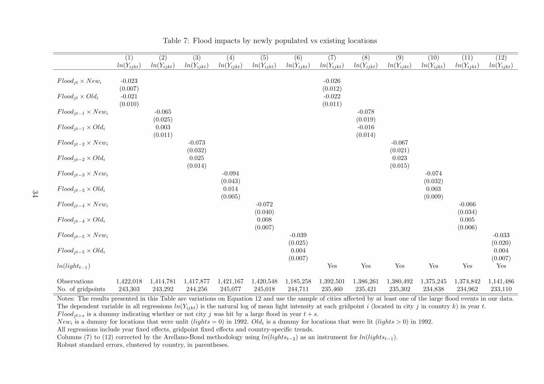
Table 7: Flood impacts by newly populated vs existing locations

(1) (2) (3) (4) (5) (6) (7) (8) (9) (10) (11) (12)ln(Yijkt) ln(Yijkt) ln(Yijkt) ln(Yijkt) ln(Yijkt) ln(Yijkt) ln(Yijkt) ln(Yijkt) ln(Yijkt) ln(Yijkt) ln(Yijkt) ln(Yijkt)

Floodjt ×Newi -0.023 -0.026(0.007) (0.012)

Floodjt ×Oldi -0.021 -0.022(0.010) (0.011)

Floodjt−1 ×Newi -0.065 -0.078(0.025) (0.019)

Floodjt−1 ×Oldi 0.003 -0.016(0.011) (0.014)

Floodjt−2 ×Newi -0.073 -0.067(0.032) (0.021)

Floodjt−2 ×Oldi 0.025 0.023(0.014) (0.015)

Floodjt−3 ×Newi -0.094 -0.074(0.043) (0.032)

Floodjt−3 ×Oldi 0.014 0.003(0.005) (0.009)

Floodjt−4 ×Newi -0.072 -0.066(0.040) (0.034)

Floodjt−4 ×Oldi 0.008 0.005(0.007) (0.006)

Floodjt−5 ×Newi -0.039 -0.033(0.025) (0.020)

Floodjt−5 ×Oldi 0.004 0.004(0.007) (0.007)

ln(lightt−1) Yes Yes Yes Yes Yes Yes

Observations 1,422,018 1,414,781 1,417,877 1,421,167 1,420,548 1,185,258 1,392,501 1,386,261 1,380,492 1,375,245 1,374,842 1,141,486No. of gridpoints 243,303 243,292 244,256 245,077 245,018 244,711 235,460 235,421 235,302 234,838 234,962 233,110

Notes: The results presented in this Table are variations on Equation 12 and use the sample of cities affected by at least one of the large flood events in our data.The dependent variable in all regressions ln(Yijkt) is the natural log of mean light intensity at each gridpoint i (located in city j in country k) in year t.Floodjt+s is a dummy indicating whether or not city j was hit by a large flood in year t + s.Newi is a dummy for locations that were unlit (lights = 0) in 1992. Oldi is a dummy for locations that were lit (lights > 0) in 1992.All regressions include year fixed effects, gridpoint fixed effects and country-specific trends.Columns (7) to (12) corrected by the Arellano-Bond methodology using ln(lightst−2) as an instrument for ln(lightst−1).Robust standard errors, clustered by country, in parentheses.

34

7 Appendix Tables

(not necessarily for publication)

35

Table A1: Light intensity by elevation, democracy and income levels

(1) (2) (3) (4) (5) (6) (7) (8) (9)ln(Yik) ln(Yik) ln(Yik) ln(Yik) ln(Yik) ln(Yik) ln(Yik) ln(Yik) ln(Yik)

Elev < 10mi 0.182 0.309 0.272 0.053 0.390 0.364 -0.028 0.004 0.024(0.037) (0.060) (0.056) (0.012) (0.389) (0.410) (0.267) (0.270) (0.209)

Elev < 10mi ×DemocracyIndicatork -0.175 -0.191 0.007 0.009 -0.225(0.067) (0.076) (0.037) (0.029) (0.078)

Elev < 10mi × ln(GDPpercapita)k -0.021 -0.023 0.009 0.005 0.028(0.037) (0.040) (0.029) (0.029) (0.023)

Observations 3,642,083 3,610,249 3,610,249 3,610,249 3,562,613 3,562,613 3,562,613 3,543,409 3,543,409Country FE Yes Yes Yes No Yes Yes No No YesCity FE No No No Yes No No Yes Yes NoRiver and Coast FE No No Yes Yes No Yes Yes Yes Yes

Notes: The regressions reported in this Table are variations on Equation 9 and include the full global sample of all urban areas.The dependent variable in all regressions ln(Yik) is the natural log of mean light intensity (measured in 2012) at each gridpoint i (located inin country k).Elev < 10mi is a dummy variable for locations that are less than 10m above sea level.ln(GDPpercapita)k is the natural log of GDP per capita (in 2011) in country k (data are from the Penn World Tables v8).DemocracyIndicatork is a dummy for countries with a Polity IV score (in 2008) greater than or equal to 5.Regressions with river and coast controls include dummies for locations within 10km of the nearest river or coast.Robust standard errors, clustered by country, in parentheses.Robust standard errors are clustered by country.

36

Table A2: Main effects of flood on light, city-year panel

(1) (2) (3) (4) (5) (6)ln(Yjkt) ln(Yjkt) ln(Yjkt) ln(Yjkt) ln(Yjkt) ln(Yjkt)

Floodjt -0.017 -0.019(0.007) (0.006)

Precip > 500mmlt -0.039 -0.040(0.011) (0.015)

Precip > 1000mmlt -0.057 -0.058(0.014) (0.014)

ln(lightt−1) Yes Yes Yes

Observations 10,363 10,363 10,363 9,878 9,878 9,878No. of urban areas 1,817 1,817 1,817 1,702 1,702 1,702

Notes: The results presented in this Table correspond to Equation 11 and usethe sample of cities affected by at least one of the large flood events in our data.The dependent variable in all regressions ln(Yjkt) is the natural log of mean lightintensity for each city j (located in country k) in year t.Floodjt is a dummy indicating whether or not city j was hit by a large floodin year t.Precip > 1000mmlt (> 500mmlt) indicates locations that experienced monthlyprecipitation of 1000mm (500mm) or more in year t.All regressions include year fixed effects, city fixed effects andcountry-specific trends.Columns (4) to (6) corrected by the Arellano-Bond methodology usingln(lightst−2) as an instrument for ln(lightst−1).Robust standard errors, clustered by country, in parentheses.

37

Table A3: Recovery, gridpoint year panel, extreme precipitation (500mm) indicator

(1) (2) (3) (4) (5) (6) (7) (8) (9) (10)ln(Yijkt) ln(Yijkt) ln(Yijkt) ln(Yijkt) ln(Yijkt) ln(Yijkt) ln(Yijkt) ln(Yijkt) ln(Yijkt) ln(Yijkt)

Precip > 500mmjt -0.025 -0.027(0.008) (0.008)

Precip > 500mmjt−1 0.004 0.003(0.012) (0.011)

Precip > 500mmjt−2 0.002 0.003(0.006) (0.007)

Precip > 500mmjt−3 -0.013 -0.012(0.012) (0.012)

Precip > 500mmjt−4 -0.009 -0.009(0.010) (0.010)

ln(lightt−1) Yes Yes Yes Yes Yes

Observations 1,422,018 1,422,018 1,422,018 1,422,018 1,422,018 1,392,501 1,392,501 1,392,501 1,392,501 1,392,501No. of gridpoints 243,303 243,303 243,303 243,303 243,303 235,460 235,460 235,460 235,460 235,460

Notes: The results in this Table are variations on Equation 10 and use the sample of cities affected by at least one of the largeflood events in our data.The dependent variable in all regressions ln(Yijkt) is the natural log of mean light intensity at each gridpoint i (located in city jin country k) in year t.Floodjt+s is a dummy indicating whether or not city j was hit by a large flood in year t + s.Precip > 500mmjt+s indicates locations that experienced monthly precipitation of 500mm or more in year t + s.All regressions include year fixed effects, gridpoint fixed effects and country-specific trends.Columns (6) to (10) corrected by the Arellano-Bond methodology using ln(lightst−2) as an instrument for ln(lightst−1).Robust standard errors, clustered by country, in parentheses.

38

Table A4: Recovery, gridpoint year panel, extreme precipitation (1000mm) indicator

(1) (2) (3) (4) (5) (6) (7) (8) (9) (10)ln(Yijkt) ln(Yijkt) ln(Yijkt) ln(Yijkt) ln(Yijkt) ln(Yijkt) ln(Yijkt) ln(Yijkt) ln(Yijkt) ln(Yijkt)

Precip > 1000mmjt -0.080 -0.083(0.018) (0.018)

Precip > 1000mmjt−1 0.054 0.053(0.033) (0.034)

Precip > 1000mmjt−2 0.004 0.002(0.020) (0.019)

Precip > 1000mmjt−3 0.002 0.004(0.013) (0.012)

Precip > 1000mmjt−4 0.001 0.003(0.029) (0.028)

ln(lightt−1) Yes Yes Yes Yes Yes

Observations 1,422,018 1,422,018 1,422,018 1,422,018 1,422,018 1,392,501 1,392,501 1,392,501 1,392,501 1,392,501No. of gridpoints 243,303 243,303 243,303 243,303 243,303 235,460 235,460 235,460 235,460 235,460

Notes: The results in this Table are variations on Equation 10 and use the sample of cities affected by at least one of the largeflood events in our data.The dependent variable in all regressions ln(Yijkt) is the natural log of mean light intensity at each gridpoint i (located in city jin country k) in year t.Floodjt+s is a dummy indicating whether or not city j was hit by a large flood in year t + s.Precip > 1000mmjt+s indicates locations that experienced monthly precipitation of 1000mm or more in year t + s.All regressions include year fixed effects, gridpoint fixed effects and country-specific trends.Columns (6) to (10) corrected by the Arellano-Bond methodology using ln(lightst−2) as an instrument for ln(lightst−1).Robust standard errors, clustered by country, in parentheses.

39

Table A5: Recovery, city-year panel

(1) (2) (3) (4) (5) (6) (7) (8) (9) (10)ln(Yjkt) ln(Yjkt) ln(Yjkt) ln(Yjkt) ln(Yjkt) ln(Yjkt) ln(Yjkt) ln(Yjkt) ln(Yjkt) ln(Yjkt)

Floodjt -0.017 -0.019(0.007) (0.006)

Floodjt−1 -0.003 -0.008(0.014) (0.019)

Floodjt−2 0.017 0.017(0.016) (0.015)

Floodjt−3 0.004 -0.008(0.009) (0.021)

Floodjt−4 0.014 0.014(0.009) (0.011)

ln(lightt−1) Yes Yes Yes Yes Yes

Observations 10,363 10,281 10,315 10,352 10,338 9,878 9,869 9,833 9,785 9,796No. of urban areas 1,817 1,814 1,820 1,818 1,819 1,702 1,707 1,707 1,703 1,712

Notes: The results presented in this Table correspond to Equation 11 and use the sample of cities affected by at least oneof the large flood events in our data.The dependent variable in all regressions ln(Yjkt) is the natural log of mean light intensity in each city j (located incountry k) in year t.Floodjt+s is a dummy indicating whether or not city j was hit by a large flood in year t + s.All regressions include year fixed effects, city fixed effects and country-specific trends.Columns (6) to (10) corrected by the Arellano-Bond methodology using ln(lightst−2) as an instrument for ln(lightst−1).Robust standard errors, clustered by country, in parentheses.

40

Table A6: Interactions with elevation, extreme precipitation (1000mm) indicator

(1) (2) (3) (4) (5) (6) (7) (8) (9)ln(Yijkt) ln(Yijkt) ln(Yijkt) ln(Yijkt) ln(Yijkt) ln(Yijkt) ln(Yijkt) ln(Yijkt) ln(Yijkt)

Precip > 1000mmjt × elev<10i -0.120 -0.122 -0.100(0.019) (0.020) (0.016)

Precip > 1000mmjt × elev10+i -0.052 -0.056 -0.031(0.022) (0.021) (0.011)

Precip > 1000mmjt−1 × elev<10i 0.111 0.111 0.117(0.015) (0.016) (0.017)

Precip > 1000mmjt−1 × elev10+i 0.020 0.018 0.033(0.035) (0.035) (0.030)

Precip > 1000mmjt−2 × elev<10i 0.006 0.007 -0.022(0.009) (0.014) (0.011)

Precip > 1000mmjt−2 × elev10+i 0.003 0.001 -0.005(0.028) (0.026) (0.023)

ln(lightt−1) Yes Yes Yes

Observations 1,422,018 1,422,018 1,422,018 1,392,501 1,392,501 1,392,501 1,422,018 1,422,018 1,422,018No. of gridpoints 243,303 243,303 243,303 235,460 235,460 235,460 243,303 243,303 243,303

Notes: The results presented in this Table correspond to Equation 12 and use the sample of cities affected by at least one ofthe large flood events in our data.The dependent variable in all regressions ln(Yijkt) is the natural log of mean light intensity at each gridpoint i (located incity j in country k) in year t.Precip > 1000mmlt+s indicates locations that experienced monthly precipitation of 1000mm or more in year t+ s.Elevationh is a dummy for elevation band h, where h is either less than 10m above sea level, or 10m or more above sea level.All regressions include year fixed effects and gridpoint fixed effects.Columns (1) to (6) include country-specific trends. Columns (7) to (9) include city-specific trends.Columns (4) to (6) corrected by the Arellano-Bond methodology using ln(lightst−2) as an instrument for ln(lightst−1).Robust standard errors, clustered by country, in parentheses.

41

Table A7: Interactions with elevation, excluding locations within 10km of rivers and coasts

(1) (2) (3) (4) (5) (6)ln(Yijkt) ln(Yijkt) ln(Yijkt) ln(Yijkt) ln(Yijkt) ln(Yijkt)

Floodjt × elev<10i -0.030 -0.032(0.007) (0.006)

Floodjt × elev10+i -0.020 -0.021(0.013) (0.014)

Floodjt−1 × elev<10i 0.015 -0.009(0.011) (0.011)

Floodjt−1 × elev10+i -0.001 -0.016(0.012) (0.017)

Floodjt−2 × elev<10i 0.037 0.038(0.017) (0.017)

Floodjt−2 × elev10+i 0.017 0.017(0.014) (0.014)

ln(lightt−1) Yes Yes Yes

Observations 814,294 810,524 812,476 795,536 792,801 790,097No. of gridpoints 139,712 139,683 140,298 134,640 134,600 134,474

Notes: The results presented in this Table correspond to Equation 12 and use thesample of cities affected by at least one of the large flood events in our data,restricted to exclude gridpoints within 10km of the nearest river or coast.The dependent variable in all regressions ln(Yijkt) is the natural log of mean lightintensity at each gridpoint i (located in city j in country k) in year t.Floodjt+s is a dummy indicating whether or not city j was hit by a large floodin year t+ s.Elevationh is a dummy for elevation band h, where h is eitherless than 10m above sea level, or 10m or more above sea level.All regressions include year fixed effects and gridpoint fixed effectsand country-specific trends.Columns (4) to (6) corrected by the Arellano-Bond methodology using ln(lightst−2)as an instrument for ln(lightst−1).Robust standard errors, clustered by country, in parentheses.

42

Table A8: Interactions with elevation, excluding cities entirely less than 10m above sea level

(1) (2) (3) (4) (5) (6)ln(Yijkt) ln(Yijkt) ln(Yijkt) ln(Yijkt) ln(Yijkt) ln(Yijkt)

Floodjt × elev<10i -0.021 -0.022(0.006) (0.007)

Floodjt × elev10+i -0.019 -0.020(0.012) (0.012)

Floodjt−1 × elev<10i 0.012 -0.006(0.008) (0.010)

Floodjt−1 × elev10+i -0.007 -0.022(0.014) (0.018)

Floodjt−2 × elev<10i 0.046 0.045(0.016) (0.016)

Floodjt−2 × elev10+i 0.007 0.007(0.011) (0.011)

ln(lightt−1) Yes Yes Yes

Observations 1,379,280 1,372,088 1,375,024 1,351,484 1,345,342 1,339,592No. of gridpoints 235,874 235,861 236,793 228,408 228,358 228,261

Notes: The results presented in this Table correspond to Equation 12 and use thesample of cities affected by at least one of the large flood events in our data,restricted to exclude cities that are entirely less than 10m above sea level.The dependent variable in all regressions ln(Yijkt) is the natural log of mean lightintensity at each gridpoint i (located in city j in country k) in year t.Floodjt+s is a dummy indicating whether or not city j was hit by a large floodin year t + s.Elevationh is a dummy for elevation band h, where h is eitherless than 10m above sea level, or 10m or more above sea level.All regressions include year fixed effects and gridpoint fixed effectsand country-specific trends.Columns (4) to (6) corrected by the Arellano-Bond methodology using ln(lightst−2)as an instrument for ln(lightst−1).Robust standard errors, clustered by country, in parentheses.

43

CENTRE FOR ECONOMIC PERFORMANCE Recent Discussion Papers

1397 Lorenzo Caliendo Giordano Mion Luca David Opromolla Esteban Rossi-Hansberg

Productivity and Organization in Portuguese Firms

1396 Richard Murphy Gill Wyness

Testing Means-Tested Aid

1395 Zack Cooper Stuart Craig Martin Gaynor John Van Reenen

The Price Ain’t Right? Hospital Prices and Health Spending on the Privately Insured

1394 Hannes Schwandt Amelie Wuppermann

The Youngest Get the Pill: Misdiagnosis and the Production of Education in Germany

1393 Yatang Lin Yu Qin Zhuan Xie

International Technology Transfer and Domestic Innovation: Evidence from the High-Speed Rail Sector in China

1392 Robin Naylor Jeremy Smith Shqiponja Telhaj

Graduate Returns, Degree Class Premia and Higher Education Expansion in the UK

1391 Marc Fleurbaey Hannes Schwandt

Do People Seek To Maximize Their Subjective Well-Being?

1390 Benjamin R. Handel Jonathan T. Kolstad Johannes Spinnewijn

Information Frictions and Adverse Selection: Policy Interventions in Health Insurance Markets

1389 Kilian Huber The Persistence of a Banking Crisis

1388 Francesco Caselli Miklos Koren Milan Lisicky Silvana Tenreyro

Diversification through Trade

1387 Hannes Schwandt Janet Currie

Short and Long-Term Effects of Unemployment on Fertility

1386 Marta De Philippis Multitask Agents and Incentives: The Case of Teaching and Research for University Professors

1385 Ferdinando Monte Stephen J. Redding Esteban Rossi-Hansberg

Commuting, Migration and Local Employment Elasticities

1384 Tito Boeri Juan Francisco Jimeno

The Unbearable Divergence of Unemployment in Europe

1383 Sarah Flèche Distaste for Centralization: Evidence from a Quasi-Natural Experiment in Switzerland

1382 Johannes Boehm The Impact of Contract Enforcement Costs on Outsourcing and Aggregate Productivity

1381 Andrew B. Bernard Swati Dhingra

Contracting and the Division of the Gains from Trade

1380 Warn N. Lekfuangfu Nattavudh Powdthavee Andrew E. Clark George Ward

Early Maternal Employment and Non-cognitive Outcomes in Early Childhood and Adolescence: Evidence from British Birth Cohort Data

1379 Scott R. Baker Nicholas Bloom Steven J. Davis

Measuring Economic Policy Uncertainty

1378 Holger Breinlich Volker Nocke Nicolas Schutz

Merger Policy in a Quantitative Model of International Trade

1377 Kalina Manova Zhihong Yu

How Firms Export: Processing vs. Ordinary Trade With Financial Frictions

1376 Jordi Blanes i Vidal Tom Kirchmaier

The Effect of Police Response Time on Crime Detection

The Centre for Economic Performance Publications Unit Tel 020 7955 7673 Fax 020 7404 0612

Email info@cep.lse.ac.uk Web site http://cep.lse.ac.uk