LS2W: Implementing the Locally Stationary 2D Wavelet ... · LS2W: Implementing the Locally Stationary 2D ... in Sections3and Section4provides a tutorial ... Implementing the Locally

JSS Journal of Statistical SoftwareJuly 2011, Volume 43, Issue 3. http://www.jstatsoft.org/

LS2W: Implementing the Locally Stationary 2D

Wavelet Process Approach in R

Idris A. EckleyLancaster University

Guy P. NasonUniversity of Bristol

Abstract

Locally stationary process representations have recently been proposed and applied toboth time series and image analysis applications. This article describes an implementationof the locally stationary two-dimensional wavelet process approach in R. This package per-mits construction of estimates of spatially localized spectra and localized autocovariancewhich can be used to characterize structure within images.

Keywords: random field, locally stationary, local autocovariance, LS2W, texture analysis,non-decimated wavelets, R.

1. Introduction

Wavelet techniques have established themselves in the statistics literature as a popular ap-proach for nonparametric curve estimation and for the modelling, analysis and forecasting oftime series. Given the (typically) inherent non-stationary nature of time series, the modellingof locally stationary processes has received increased attention in recent years. Nason, vonSachs, and Kroisandt (2000, henceforth referred to as NvSK) provide an early contributionto this field, introducing a class of locally stationary wavelet (LSW) processes together withan associated estimation scheme. Other recent contributions include Fryzlewicz and Nason(2006), who propose a new technique for estimating the evolutionary wavelet spectrum basedon the Haar-Fisz transform. Van Bellegem and von Sachs (2008) extend the class of LSW pro-cesses to contain processes whose spectral density can change suddenly in time. Van Bellegemand Dahlhaus (2006) propose an estimation approach to fit time-varying models to an alter-native clasfigs of locally stationary processes using the Whittle likelihood, whilst Dahlhausand Polonik (2009) apply empirical process methodology to locally stationary time seriesprocesses.

http://www.jstatsoft.org/

2 LS2W: Locally Stationary 2D Wavelet Processes in R

This article introduces the LS2W package which provides an implementation of the mod-elling approach proposed by Eckley, Nason, and Treloar (2010) for locally stationary spatialcovariance structure of (regular) lattice processes, such as images. The approach, which isan extension of NvSK’s time series modelling paradigm, is in part motivated by a frequentlyhighlighted aspect of image texture, namely that texture possesses structure on many differentscales. Moreover, several researchers have highlighted that the human and mammalian visualsystems process images in a multiscale manner, preserving both local and global information(see for example Daugman 1990 or Field 1999). Thus there is a compelling argument for thedevelopment of a multiscale model of image texture as proposed by Eckley et al. (2010).

The LS2W package has been developed in R (R Development Core Team 2011) and makesuse of several functions within the wavethresh package developed by Nason (2010). Bothpackages are available from the Comprehensive R Archive Network (CRAN) at http://CRAN.R-project.org/.

Our article is organized as follows: Section 2 provides a brief introduction to wavelets, payingparticular attention to the discrete wavelets which form the central building block of the locallystationary two-dimensional wavelet (LS2W) approach. The modelling approach is introducedin Sections 3 and Section 4 provides a tutorial on the LS2W package whilst describing variouselements of the estimation scheme established by Eckley et al. (2010). Finally a case studyinvolving texture discrimination is provided in Section 5.

2. A brief introduction to wavelets

Wavelet research has undergone a rapid expansion in terms of volume and complexity inthe last 20 years although the basic concepts are extremely simple. We provide a very briefintroduction to wavelets here. Those interested in learning more can consult any number ofuseful texts including Daubechies (1992), Mallat (1999), Vidakovic (1999) or Nason (2008).

For functions, f(x), on the real line, the idea is that there exists a basis of functions,{ψjk(x)}j,k∈Z, so that

f(x) =∑j,k

dj,kψjk(x).

If the basis functions are orthogonal then the coefficients can be obtained from the functionf in the usual way, i.e.,

djk =

∫f(x)ψjk(x) dx, (1)

where j, k ∈ Z. Wavelets provide a multiscale analysis of functions, f , because the basisfunctions are all scalings of one function, ψ(x), called the mother wavelet. Such scalings aredefined by the following relation:

ψjk(x) = 2j/2ψ(2jx− k),

for all x ∈ R and j, k ∈ Z. The mother wavelet is chosen to have several important propertiessuch as fast decay (often compact support), oscillation, zero integral and not least that thewavelets form an (orthonormal) basis. With this construction it can be seen that the coefficientdjk in (1) conveys information about the function f at a scale proportional to 2j and locationnear to 2−jk. In other words, the set of wavelet coefficients of a function characterize thefunction’s behavior at different scales and locations.

http://CRAN.R-project.org/

http://CRAN.R-project.org/

Journal of Statistical Software 3

As well as a mother wavelet one can define a father wavelet, φ(x), which is similar to akernel function such as that used in kernel density estimation or regression. Whilst waveletcoefficients provide information about the local oscillatory behavior of a function the fathercoefficients encapsulate information about the multiscale mean behavior of that function. Thefather wavelets satisfy a multiscale relation, called the dilation equation:

φ(x) =∑k

hkφ(2x− k),

for all x ∈ R. The mother wavelet ψ(x) satisfies a similar equation:

ψ(x) =∑k

gkψ(2x− k) ∀x ∈ R.

More details and illustrations of various wavelets can be found in Daubechies (1992), Mallat(1999), Vidakovic (1999) or Nason (2008). The whole set of mother/father wavelets can becharacterized by a suitable choice of hk and gk. There are many families of wavelets but aparticularly useful and famous set, compactly supported, was developed by Daubechies (1988)which we will use extensively here. Daubechies’ construction produced sets of hk, gk knownas quadrature mirror filters.

The relationship between the mother and father wavelets lies as the heart of the wavelet trans-form. For a thorough discussion we refer the reader to Nason (2008). Of particular relevanceto the work in this paper, both the mother and father wavelet are required to construct the(separable) two-dimensional wavelet transform which we use as the basic building block in ourlocally stationary modelling framework. In the next section we describe this two-dimensionalwavelet transform.

2.1. Discrete wavelets

In many real-life situations data appear not as continuous mathematical functions but discretesequences. Hence, a discrete wavelet transform, with “discrete wavelets” exists to providediscrete wavelet coefficients. One of the appealing features of such a transform is the existenceof an extremely fast and efficient transform algorithm, such as that proposed by Mallat (1989).Mallat’s discrete wavelet transform achieves a computational effort which is linear in thenumber of data points.

Let {hk} and {gk} be the low and high pass quadrature mirror filters that are used in theconstruction of the Daubechies (1992) compactly supported continuous time wavelets. NvSKdefine the associated discrete father wavelet filters, φj = (φj,0, . . . , φj,(Lj−1)) which are vectorsof length Lj for integer scales j > 0 and obtained using the formulae:

φ1,n = hn, for n = 0, . . . , L1 − 1, (2)

φ(j+1),n =∑k

hn−2kφj,k, for n = 0, . . . , Lj+1 − 1, (3)

where Lj = (2j − 1)(Nh − 1) + 1, Nh is the number of non-zero elements of {hk} and δ0kis the Kronecker delta. This definition for discrete father wavelet filters is essentially thesame as for mother wavelets, ψj , given in NvSK, except that the hn−2k in (2) is replacedby gn−2k. Also, here we adopt positive scales rather than use the notationally inconvenient


j < 0 as in NvSK. As an example, the discrete Haar father wavelet filters at scales 1 and 2are φ1 = (h0, h1) = (1/

√2)(1, 1) and φ2 = (h20, h1h0, h0h1, h

21) = 1

2(1, 1, 1, 1).

Two-dimensional discrete father wavelet filters can be formed from one-dimensional motherand father wavelet filters by a tensor product operation as follows.

Definition 1. Let k = (k1, k2) where k1, k2 ∈ Z. We define the two-dimensional discretewavelet filters, {ψlj}, as finite matrices of dimension L2

j , as follows:

ψlj =

ψlj,(0,0) · · · ψlj,(0,Lj−1)...

......

ψlj,(Lj−1,0) · · · ψlj,(Lj−1,Lj−1)

for l = h, v or d.

Here h, v and d denote the horizontal, vertical and diagonal directions. The elements of thematrix are defined by

ψhj,k = φj,k1ψj,k2ψvj,k = ψj,k1φj,k2

and ψdj,k = ψj,k1ψj,k2

for k1, k2 = 0, . . . , Lj − 1, (4)

where ψj,k and φj,k are the one-dimensional discrete wavelets. Similarly, the two-dimensionaldiscrete father wavelet filter is defined as:

φj,k = φj,k1φj,k2 .

2.2. Example: Discrete Haar wavelets

The finest scale discrete Haar wavelet in the diagonal decomposition direction is given by:

ψd1 = ψ1 ⊗ ψ1 =1

2

[1 −1−1 1

];

where ⊗ is the tensor product. The second finest scale discrete Haar wavelet in the horizontaldirection is given by:

ψh2 = φ2 ⊗ ψ2 =1

4

1 1 −1 −11 1 −1 −11 1 −1 −11 1 −1 −1

.For convenience, we will henceforth refer to these discrete wavelet filters as simply discretewavelets.

As with the one-dimensional case, considered by NvSK, we can form the collection of non-decimated discrete wavelets by translations as follows:

ψlj,u(r) = ψlj,u−r

for every scale j, direction l and locations u, r ∈ Z2. Thus with two-dimensional non-decimated wavelets there is a wavelet at each scale, direction and location. For further detailson non-decimated wavelets and their associated transform see Nason and Silverman (1995)or Nason (2008).


3. The LS2W approach

3.1. Motivation

Suppose that we have a random field which is defined on a regular grid, {Xr}r∈Z2 for whichwe wish to estimate the covariance COV(Xr, Xs) = γr,s where r, s ∈ Z2. The covariancestructure of such a field could take many possible forms. For example, the process could be(second-order) stationary, or intrinsically stationary (see Priestley 1981 or Cressie 1991) or inextreme cases the covariance could possess minimal controls such as γr,s = γt,u if and only ifr = t and s = u. This last case permits the covariance to change from location to location in ahighly nonstationary manner. Clearly, statistical estimation in this situation is troublesome.

The form of covariance structure that Eckley et al. (2010) consider lies somewhere between thetwo extremes of stationarity and the highly nonstationary form. They permit the covariancestructure to change slowly as a function of location and hence the covariance structure arounda particular location, r, may be estimated by pooling information from data close to r. Fieldswhich exhibit this slowly varying structure are termed locally stationary random fields. Sincemany real-life images have a locally stationary structure operating at several different scales,Eckley et al. (2010) adopt wavelets as the basic building block for such locally stationaryprocesses.

3.2. The model

Armed with the non-decimated discrete wavelet building blocks of Section 2.1, we now intro-duce the wavelet model for random fields proposed by Eckley et al. (2010).

Definition 2. Let R = (R,S) where R = 2m, S = 2n ≥ 1 for m,n ∈ N and set J(R,S) ≡log2{min(R,S)}. Further, let r = (r, s) and u = (u, v) for r,u ∈ [0, R − 1] × [0, S − 1].Then a class of locally stationary two-dimensional wavelet processes (LS2W) is defined to bea sequence of stochastic processes which lie on a regular grid denoted by

{Xr;R}r∈[0,R−1]×[0,S−1].

Such processes have the following representation in the mean-square sense:

Xr;R =∑l

∞∑j=1

∑u

wlj,u;Rψlj,u(r)ξlj,u, (5)

where the sum over l is over decomposition directions v, h and d, {ψlj,u(r)} is a collection of

discrete non-decimated two-dimensional wavelets and ξlj,u is a mean zero, random orthonormal

increment process satisfying E(ξlj,kξ

pm,n

)= δj,mδk,nδl,p, (i.e., is uncorrelated).

Eckley et al. (2010) also impose certain technical assumptions on the LS2W processes. Theseprovide control mechanisms over the degree of non-stationary structure allowed within suchmodels, imposing zero mean and the finiteness of the model.


3.3. Example: Haar moving average fields

As an example we use Haar wavelets to construct LS2W fields. We begin by defining thecanonical set of fields from which more complicated processes can be constructed.

Definition 3. Let c ∈ R and r = (r, s). We define a Haar MA field of order j0, in direction

l0, to be the LS2W process Xj0,l0r generated by the Haar 2D non-decimated discrete wavelets

with the following condition on the amplitude:

wlj,u =

{c for j = j0, l = l0,0 otherwise.

For example, setting c = σ in the definition for j0 = 1 and l0 = d (diagonal direction), usingHaar wavelets and setting the orthonormal increment sequence ξd1,u = εu where {εu} is apurely random process with mean zero and variance 1 gives

X1,dr = σ

∑u

ψd1,u−rξd1,u = σ(εr,s − εr,s+1 − εr+1,s + εr+1,s+1)/2. (6)

Haar MA fields are special cases of the moving average fields due to Haining (1978) – seeMoore 1988 or Cressie 1991 for further details.

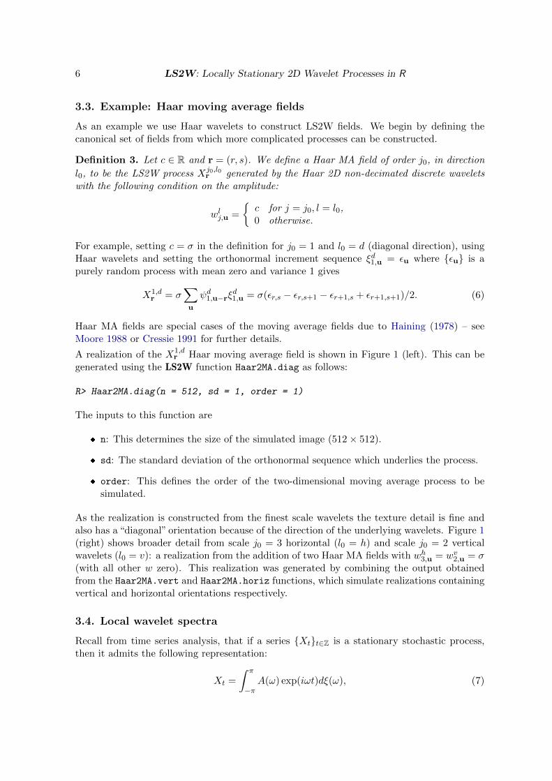
A realization of the X1,dr Haar moving average field is shown in Figure 1 (left). This can be

generated using the LS2W function Haar2MA.diag as follows:

R> Haar2MA.diag(n = 512, sd = 1, order = 1)

The inputs to this function are

� n: This determines the size of the simulated image (512× 512).

� sd: The standard deviation of the orthonormal sequence which underlies the process.

� order: This defines the order of the two-dimensional moving average process to besimulated.

As the realization is constructed from the finest scale wavelets the texture detail is fine andalso has a “diagonal” orientation because of the direction of the underlying wavelets. Figure 1(right) shows broader detail from scale j0 = 3 horizontal (l0 = h) and scale j0 = 2 verticalwavelets (l0 = v): a realization from the addition of two Haar MA fields with wh3,u = wv2,u = σ(with all other w zero). This realization was generated by combining the output obtainedfrom the Haar2MA.vert and Haar2MA.horiz functions, which simulate realizations containingvertical and horizontal orientations respectively.

3.4. Local wavelet spectra

Recall from time series analysis, that if a series {Xt}t∈Z is a stationary stochastic process,then it admits the following representation:

Xt =

∫ π

−πA(ω) exp(iωt)dξ(ω), (7)


Figure 1: Haar moving average fields. Left: 2D Haar moving average field of order 1 withdiagonal detail only. Right: A LS2W process with contributions at scales 2 and 3 in thevertical and horizontal directions respectively.

where A(ω) denotes the amplitude of the process and dξ(ω) is an orthonormal increments pro-cess (see Priestley 1981 for further details). Here the amplitude A(ω) controls the magnitudeof the sinusoidal oscillation at frequency ω. The traditional way of presenting the amplitudeis the spectrum: f(ω) = |A(ω)|2. Equivalent structures also exist in the stationary randomfield setting. It is natural therefore to consider what the LS2W analogue of such a quantitymight be.

To this end, we introduce the local wavelet spectrum for a LS2W process Xr:

Slj(z) = Slj(z1, z2) = limmin{R,S}→∞

|wlj,[z1R],[z2S]|2 (8)

for z ∈ (0, 1)2, j ∈ 1, . . . , J , and l ∈ {h, v or d}.In other words, the LWS delivers a location-direction/scale decomposition of structure (i.e.,variance) within a LS2W process. Note that in this definition we use a quantity z, knownas rescaled location. Such rescaling is common within the locally stationary literature. Forfurther details in the locally stationary Fourier, locally stationary wavelet or LS2W settingwe refer the reader to Dahlhaus (1997), Nason et al. (2000) or Eckley (2001) respectively.

3.5. Example

Let us reconsider the stationary, Haar MA field, example considered in Section 3.3. For aprocess of the form X1,d

r , it is easily verified that the LWS takes the form:

Slj(z) = |wlj,([z1R],[z2S])|2;

=

{σ2 for j = 1 and l = d0 otherwise;

= σ2δj,1δl,d ∀ z ∈ (0, 1)2.


3.6. Local autocovariance and autocorrelation wavelets

For stationary processes it is well-known that the covariance is the Fourier transform of thespectrum. For completeness, we highlight that an equivalent relationship also exists in theLS2W setting. Prior to this we introduce autocorrelation wavelets. These will prove usefulin defining the wavelet-based local covariance.

We define two-dimensional autocorrelation wavelets as follows:

Definition 4. Let j ∈ N, l ∈ {v, h, d} and τ ∈ Z2. Then the autocorrelation (ac) wavelet ofa 2D discrete wavelet family {ψlj,k} is given by

Ψlj(τ ) =

∑v∈Z2

ψlj,v(0)ψlj,v(τ ). (9)

Note that the 2D ac wavelets inherit a separable form from the discrete wavelets of equa-tion (4), i.e., in the horizontal, vertical and diagonal directions:

Ψhj (τ ) = Φj(τ1)Ψj(τ2), Ψv

j (τ ) = Ψj(τ1)Φj(τ2), Ψdj (τ ) = Ψj(τ1)Ψj(τ2), (10)

where τ = (τ1, τ2), and Ψj , Φj are the 1D discrete ac wavelet and father wavelets from NvSK.

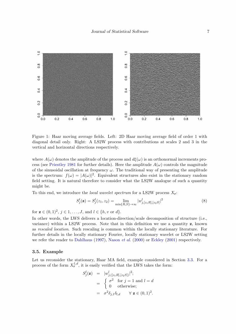
One-dimensional discrete ac wavelets can be generated using the LS2W package by callingthe PsiJ and PhiJ functions as appropriate. For example

R> MyPhi <- PhiJ(J = -4, filter.number = 1, family = "DaubExPhase")

R> plot(MyPhi[[4]], xlab = "Index", ylab = "Haar AC Scaling function")

R> MyPsi <- PsiJ(J = -4, filter.number = 1, family = "DaubExPhase")

R> plot(MyPsi[[4]], xlab = "Index", ylab = "Haar AC Wavelet")

0 5 10 15 20 25 30

0.2

0.4

0.6

0.8

1.0

Index

Haa

r A

utoc

orre

latio

n S

calin

g F

unct

ion

0 5 10 15 20 25 30

−0.

50.

00.

51.

0

Index

Haa

r A

utoc

orre

latio

n W

avel

et

Figure 2: Examples of one-dimensional autocorrelation wavelets. Left: Scale 4 Haar ac fatherwavelet. Right: Scale 4 Haar ac wavelet.


produces the fourth scale ac father and ac wavelet (see Figure 2), respectively. The inputsused within the above function calls are:

� J: The scale of the ac (father) wavelet generated. Note that to follow existing conventionswithin wavethresh, we have adopted a negative scale within the LS2W code.

� filter.number: Determines the regularity of the wavelet.

� family: Determines the family of wavelets used (either DaubExPhase or DaubLeAsymm).

For details of other optional arguments, please refer to the associated R help pages.

The 2D discrete ac father wavelet is similarly given by Φj(τ ) = Φj(τ1)Φj(τ2). Details ofthe related LS2W function are provided in Section 4 where we shall see that autocorrelationwavelets play an important role in the estimation of the LWS. However, before this, weintroduce the wavelet local covariance.

Definition 5. The wavelet local covariance (LCV), C(z, τ ), of a given LS2W process withLWS {Slj(z)} is defined to be

C(z, τ ) =∑l

∞∑j=1

Slj(z)Ψlj(τ), (11)

where τ ∈ Z2 and z ∈ (0, 1)2.

To date, there has been limited research into the behavior and estimation of the wavelet LCV.More details can be found in Section 2.6 of Eckley et al. (2010), who describe the asymptoticbehavior of the LCV and establish the existence of an “inverse formula”.

4. The LS2W package

The LS2W package implements the estimation scheme described in previous sections. Itmakes use of various algorithms contained within the wavethresh package. Below we providebrief descriptions of the main functions contained within the package:

� PhiJ: Computes discrete autocorrelation father wavelets. These are automaticallystored within the R session, using a naming convention governed by Phi1Dname.

� PsiJ: Computes discrete autocorrelation mother wavelets. These are automaticallystored within the R session, using a naming convention governed by Psi1Dname.

� D2ACW: Computes two-dimensional autocorrelation wavelets. These are autmoaticallystored within the R session, using a naming convention governed by Psi2Dname.

� D2autoplot: Can be used to generate images of two-dimensional discrete autocorrela-tion wavelets.

� D2Amat: Computes the inner product matrix of two-dimensional discrete autocorrelationwavelets. These objects are automatically stored within a session following a namingconvention governed by A2name.


� cddews: Computes the local wavelet spectrum estimate as described in Eckley et al.(2010), returning an object of class cddews.

� specplot: Plots the local wavelet periodogram associated with a cddews object.

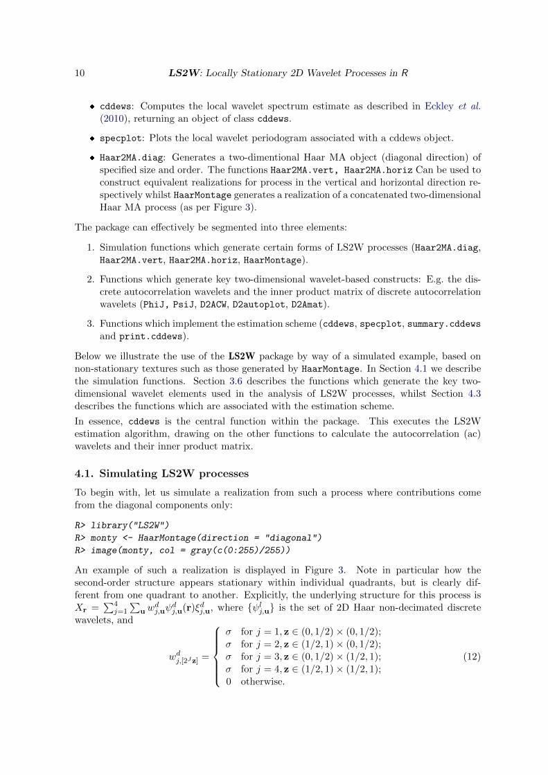
� Haar2MA.diag: Generates a two-dimentional Haar MA object (diagonal direction) ofspecified size and order. The functions Haar2MA.vert, Haar2MA.horiz Can be used toconstruct equivalent realizations for process in the vertical and horizontal direction re-spectively whilst HaarMontage generates a realization of a concatenated two-dimensionalHaar MA process (as per Figure 3).

The package can effectively be segmented into three elements:

1. Simulation functions which generate certain forms of LS2W processes (Haar2MA.diag,Haar2MA.vert, Haar2MA.horiz, HaarMontage).

2. Functions which generate key two-dimensional wavelet-based constructs: E.g. the dis-crete autocorrelation wavelets and the inner product matrix of discrete autocorrelationwavelets (PhiJ, PsiJ, D2ACW, D2autoplot, D2Amat).

3. Functions which implement the estimation scheme (cddews, specplot, summary.cddewsand print.cddews).

Below we illustrate the use of the LS2W package by way of a simulated example, based onnon-stationary textures such as those generated by HaarMontage. In Section 4.1 we describethe simulation functions. Section 3.6 describes the functions which generate the key two-dimensional wavelet elements used in the analysis of LS2W processes, whilst Section 4.3describes the functions which are associated with the estimation scheme.

In essence, cddews is the central function within the package. This executes the LS2Westimation algorithm, drawing on the other functions to calculate the autocorrelation (ac)wavelets and their inner product matrix.

4.1. Simulating LS2W processes

To begin with, let us simulate a realization from such a process where contributions comefrom the diagonal components only:

R> library("LS2W")

R> monty <- HaarMontage(direction = "diagonal")

R> image(monty, col = gray(c(0:255)/255))

An example of such a realization is displayed in Figure 3. Note in particular how thesecond-order structure appears stationary within individual quadrants, but is clearly dif-ferent from one quadrant to another. Explicitly, the underlying structure for this process isXr =

∑4j=1

∑uw

dj,uψ

dj,u(r)ξdj,u, where {ψlj,u} is the set of 2D Haar non-decimated discrete

wavelets, and

wdj,[2Jz] =

σ for j = 1, z ∈ (0, 1/2)× (0, 1/2);σ for j = 2, z ∈ (1/2, 1)× (0, 1/2);σ for j = 3, z ∈ (0, 1/2)× (1/2, 1);σ for j = 4, z ∈ (1/2, 1)× (1/2, 1);0 otherwise.

(12)


Figure 3: Simulation of a HaarMontage object.

In other words the HaarMontage code generates a simulation of concatenated HaarMA pro-cesses (see Section 3.3 for details). By construction, such images are of size 256× 256.

4.2. Two-dimensional autocorrelation wavelet generation

The concept of an ac wavelet underpins the LS2W estimation scheme. As described in Section3.6, the one-dimensional mother and father ac wavelets, Ψj and Φj , can be constructed usingthe functions PsiJ and PhiJ respectively. Recall also, from Section 2.1, that we have adopteda separable form for the two dimensional discrete wavelets. As we have previously described,the autocorrelation of these discrete wavelets is required for the correction of the (biased)raw wavelet periodograms. Consequently, the two dimensional autocorrelation wavelet alsoinherits this separability (see Eckley and Nason 2005 for further details).

To see the form of one of the autocorrelation wavelets associated with the estimation of suchLS2W processes, we can use the D2autoplot function. The main arguments which can beused within this function are:

� J: The scale of the two-dimensional ac wavelet to be generated. Again we followwavethresh’s convention by using negative numbers for this argument (-1: Fine, -J:Coarse).

� filter.number: Determines the regularity of the wavelet.

� family: Determines the family of wavelets used (DaubExPhase or DaubLeAsymm).

� direction: Determines whether the horizontal (1), vertical (2) or diagonal (3) auto-correlation wavelet is generated.


tau_1

tau_

2

AC

W coeff

2−D Autocorrelation Wavelet

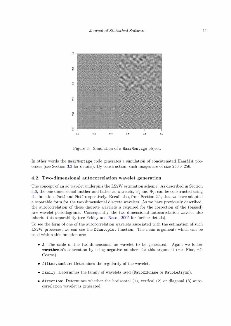
Figure 4: Example of two-dimensional Haar ac wavelet (J = −3).

� main: An overall title for the plot.

� scaling: Permits the scaling of the x and y-axes (for Haar ac wavelets only). If anyother wavelet family is used, then set scaling = "other".

Hence to generate the level 3 Haar ac wavelet in the diagonal direction (see Figure 4) wesimply issue the following command:

R> D2autoplot(J = -3, filter.number = 1, family = "DaubExPhase",

+ direction = 3, main = " ", scaling = "Haar")

Note, in particular that D2autoplot calls D2ACW to compute the 2D discrete autocorrelationwavelets. The construction method employed within D2ACW is a brute force approach – a moreelegant solution would be based on the recursive schemes as described in Eckley and Nason(2005). The routine returns only the values of the discrete ac wavelets, not their spatialpositions. Each discrete autocorrelation wavelet is compactly supported. This support isdetermined from the discrete wavelets upon which these autocorrelations are based.

As a consequence of running D2autoplot a list containing 3J ac wavelet components is re-turned. The list elements are numbered from 1 to 3J . The first J components contain thevertical autocorrelation wavelet coefficients, the second set of J components contains thehorizontal autocorrelation wavelet coefficients (scales 1, . . . , J) and the last J componentsconstitute the diagonal autocorrelation wavelet coefficients. Note that these 2D autocorre-lation wavelets are stored as matrices. The central element of the matrix refers to lag 0.To minimize future computational cost, these ac wavelet lists are automatically saved withinthe workspace using a naming convention contained within Psi2Dname. Each save objecthas three defining characteristics: Its order, filter.number and family. Each of these threecharacteristics are concatenated together to form the name returned by Psi2Dname.


As we shall see in Section 4.3 the inner product matrix of discrete autocorrelation waveletsplays a crucial role in the estimation of LS2W processes. The inner product matrix A matrixof order (3J)×(3J) containing the elements Aj,l defined in Eckley et al. (2010). Each elementis the sum over all lags of the product of the matrix coefficients of a 2D DACW matrix at levelj1 in direction l1 with that of another (not necessarily different) matrix of DACW coefficientsat level j2 in direction l2. The structure of this matrix is as follows: The rows and columnsof the matrix are labeled 1, . . . , 3J in accordance with the notation of Eckley et al. (2010).When switch = "direction" the matrix has the following structure:

� Levels 1, . . . , J correspond to the different levels of the decomposition in the verticaldirection. 1 = fine and J = coarse scale.

� Levels J + 1, . . . , 2J correspond to the different levels in the horizontal direction.

� Levels 2J + 1, . . . , 3J correspond to the different directions in the diagonal direction.

When switch = "level", the row and column elements cycle as follows: level 1 vertical, level1 horizontal, level 1 diagonal, level 2 vertical, etc.

Within LS2W an inner product matrix of two-dimensional autocorrelation wavelets can beconstructed using the function D2Amat. For example

R> D2Amat(J = -3, filter.number = 1, family = "DaubExPhase",

+ switch = "direction")

results in the following output

0 -1 -2 -3 -4 -5 -6 -7 -8

0 2.2500 1.3125 0.70312 0.2500 0.3125 0.20312 0.75000 0.9375 0.6094

-1 1.3125 4.8125 3.79687 0.3125 0.5625 0.79687 0.18750 1.3125 2.3906

-2 0.7031 3.7969 15.45312 0.2031 0.7969 1.89062 0.04687 0.4219 3.9531

-3 0.2500 0.3125 0.20312 2.2500 1.3125 0.70312 0.75000 0.9375 0.6094

-4 0.3125 0.5625 0.79687 1.3125 4.8125 3.79687 0.18750 1.3125 2.3906

-5 0.2031 0.7969 1.89062 0.7031 3.7969 15.45312 0.04687 0.4219 3.9531

-6 0.7500 0.1875 0.04687 0.7500 0.1875 0.04687 2.25000 0.5625 0.1406

-7 0.9375 1.3125 0.42187 0.9375 1.3125 0.42187 0.56250 3.0625 1.2656

-8 0.6094 2.3906 3.95312 0.6094 2.3906 3.95312 0.14062 1.2656 8.2656

We have described the above functions for completeness. However it is important to notethat it is not necessary to invoke the above functions when estimating the LWS structure ofa two-dimensional structure. All of the above functions are called automatically when thefunction cddews, which we describe in the next section, is invoked.

4.3. The estimation scheme

We now summarize the main aspects of the estimation scheme proposed by Eckley et al.(2010). To start, we define our ‘transformed’ data: the empirical wavelet coefficients of theprocess:

Definition 6. Let {Xr} be a LS2W process. Then the empirical wavelet coefficients of theprocess are given by dlj,u ≡

∑rXrψ

lj,u(r).


Input:

� A dataset consisting of a square greyscale image matrix of dimension 2J × 2J , X.

� A wavelet used to decompose the image object, ψ2d,decompose.

� A second-stage wavelet used to smooth the spectral estimate, ψ2d,smooth.

Estimation:

1. Calculate the non-decimated wavelet transform of X with respect to ψ2d,decomp.

2. Square the non-decimated detail coefficients to obtain the raw periodogram.

3. Smooth the raw periodogram using the second-stage orthonormal wavelet basisψ2d,smooth

4. Calculate the inner product matrix of discrete autocorrelation wavelets based onψ2d,decomp (A).

5. Correct the smoothed raw periodogram by applying the inverse of the inner productmatrix (A−1).

Output:

� The 3J × 2J × 2J array of the smoothed, corrected LWS estimate.

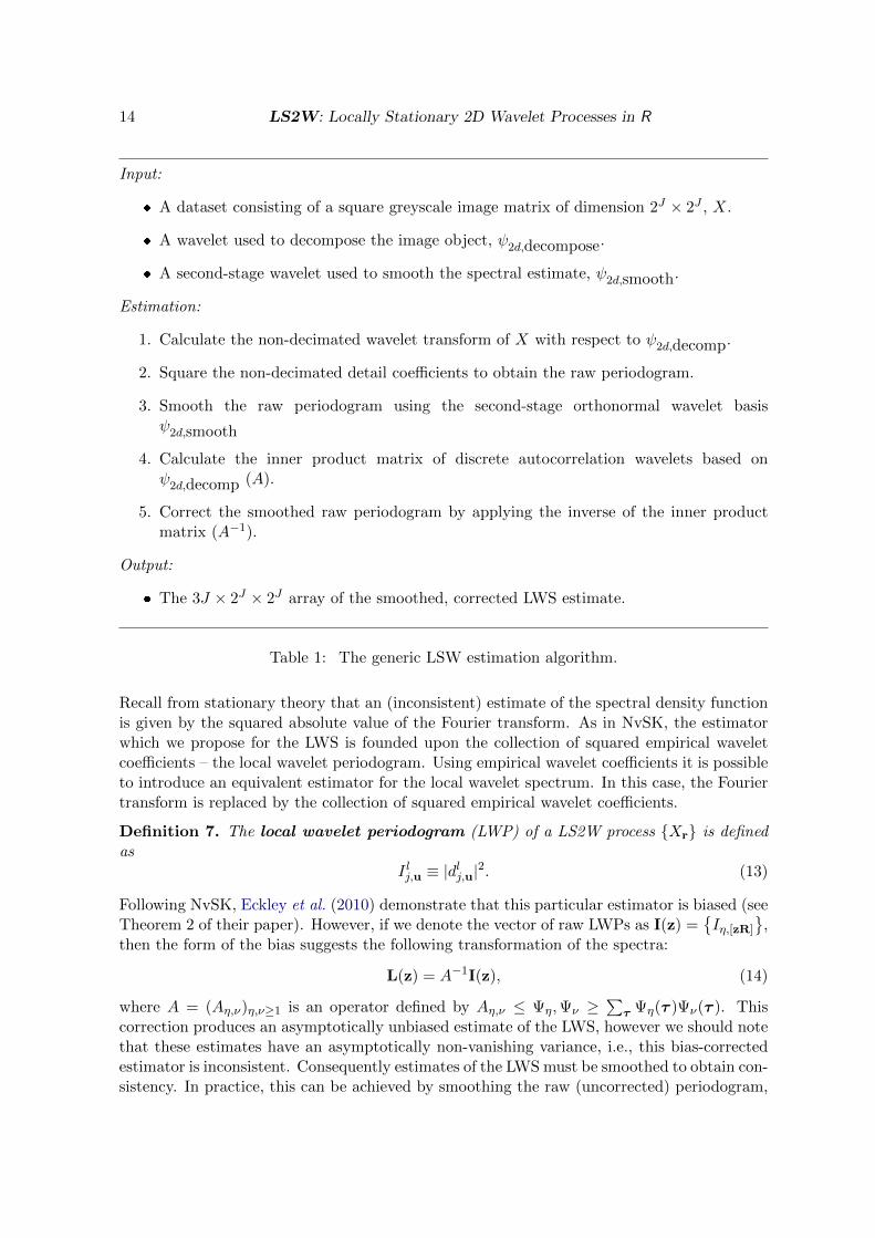
Table 1: The generic LSW estimation algorithm.

Recall from stationary theory that an (inconsistent) estimate of the spectral density functionis given by the squared absolute value of the Fourier transform. As in NvSK, the estimatorwhich we propose for the LWS is founded upon the collection of squared empirical waveletcoefficients – the local wavelet periodogram. Using empirical wavelet coefficients it is possibleto introduce an equivalent estimator for the local wavelet spectrum. In this case, the Fouriertransform is replaced by the collection of squared empirical wavelet coefficients.

Definition 7. The local wavelet periodogram (LWP) of a LS2W process {Xr} is definedas

I lj,u ≡ |dlj,u|2. (13)

Following NvSK, Eckley et al. (2010) demonstrate that this particular estimator is biased (seeTheorem 2 of their paper). However, if we denote the vector of raw LWPs as I(z) =

{Iη,[zR]

},

then the form of the bias suggests the following transformation of the spectra:

L(z) = A−1I(z), (14)

where A = (Aη,ν)η,ν≥1 is an operator defined by Aη,ν ≤ Ψη,Ψν ≥∑

τ Ψη(τ )Ψν(τ ). Thiscorrection produces an asymptotically unbiased estimate of the LWS, however we should notethat these estimates have an asymptotically non-vanishing variance, i.e., this bias-correctedestimator is inconsistent. Consequently estimates of the LWS must be smoothed to obtain con-sistency. In practice, this can be achieved by smoothing the raw (uncorrected) periodogram,


using an orthonormal second stage wavelet basis {ψl,m}, and then inverting the smoothedtransformation to obtain the smoothed estimate, Lη(z). See Eckley et al. (2010) for furtherdetails.

Pseudo-code for the above estimation scheme is provided in Table 1. Within LS2W thisestimation scheme described is contained within the function cddews. The main argumentsfor cddews are

� data: The image which you want to analyse.

� filter.number: The index of the wavelet used in the analysis of the time series (i.e.,the wavelet basis functions used to model the time series). For Daubechies compactlysupported wavelets the filter number is the number of vanishing moments.

� switch: This specifies the order of the corrected spectrum. Two options are available:The default is switch = "direction" which structures the matrix by scale within eachdecomposition direction. Thus, the ordering goes as follows (−1, V ), (−2, V ), (−3, V ), . . . .The alternative is switch = "level" structures the matrix by direction within eachscale. Thus the ordering is as follows (−1, V ), (−1, H), (−1, D), (−2, V ), (−2, H), . . . .For further details, see Eckley et al. (2010).

� correct: Eckley et al. (2010) have demonstrated that, as a consequence of the inherentredundancy of the non-decimated wavelet transform, the raw wavelet spectrum is biased.However, an asymptotically unbiased estimator may be obtained by applying the inverseof the inner product matrix of discrete autocorrelation wavelets. This logical argumentpermits the user to decide whether or not to correct for this inherent bias. By default,this is set to TRUE.

� verbose: A logical variable which allows certain informative messages to be printed onscreen. The default setting for this variable is FALSE.

� smooth: A logical variable which allows the user to specify whether or not the resultingLWP should be smoothed. It is advised that this option be set to TRUE in order thatconsistent estimates are obtained.

� sm.filter.number: Selects the index number of the wavelet that smooths each scale ofthe wavelet periodogram. A default value is provided for this variable.

� sm.family: Selects the wavelet family that smooths each scale of the wavelet peri-odogram. A default value is provided for this variable.

Example: Returning to the Haar Montage example which we considered in Section 4.1, thefinal and key step of the analysis is to estimate the LWS structure for our data, the simulatednon-stationary process, monty:

R> monty.cddews <- cddews(monty, filter.number = 1, family = "DaubExPhase")

By default, the above function will correct and smooth the LWP to obtain an (asymptoti-cally) unbiased and consistent estimate of the LWS. The resulting object monty.cddews is anexample of a cddews.object and has class cddews. The cddews class objects are returned aslists. Two methods are available for this object class : summary and print.


R> summary(monty.cddews)

Locally stationary two-dimensional wavelet decomposition structure

~~~~~~~~~~~~~~~~~~~~~~~~~~~~~~~~~~~~~~~~~~~~~~~~~~~~~~~~~~~~~~~~~~

Levels: 8

dimension of original image was: 256 x 256 pixels.

Filter family used: DaubExPhase Filter index (N): 1

Structure adopted: direction

Date: Fri Jul 15 15:56:28 2011

tells us that the dimension of the original image was 256 × 256, the analysis was performedusing the N = 1 Daubechies compactly supported wavelet from the DaubExPhase family (i.e.,Haar), and that the analysis output is structured by decomposition direction.

To discover what the monty.cddews object contains, we can use the print method:

R> print(monty.cddews)

Class 'cddews' : corrected directional dependent wavelet spectrum:

~~~~~~ : List with 14 components with names

S datadim filter.number family structure nlevels correct smooth

sm.filter.number sm.family levels type policy date

The spectrum of this image was corrected (IP matrix).

$S is a large array of data

The spectra have been smoothed to obtain consistency.

Amongst the 14 listed components, monty.cddews contains the following elements:

� S: The LWS estimate of the input data. This is a large array, the first dimension refersto a specific scale-direction pair. The next dimension refers to the rows of the spectralimage, whilst the third element refers to the columns of the image.

� datadim: The dimension of the original image.

� filter.number: The index of the wavelet used in the analysis of the image. ForDaubechies compactly supported wavelets the filter number is the number of vanishingmoments.

� family: The wavelet family used in the analysis of the image (i.e., the wavelet familyused in the modelling).

� structure: Explains the structure of the inner product matrix and S. It can only taketwo values, direction and scale.

� nlevels: The number of levels in the decomposition.

� correct: TRUE or FALSE, depending on whether the user corrected for the bias.

� Smooth: TRUE or FALSE, depending on whether the LWP has been smoothed.

� policy: The smoothing policy adopted.


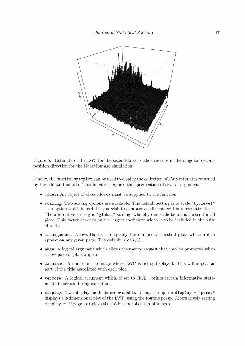
Figure 5: Estimate of the LWS for the second-finest scale structure in the diagonal decom-position direction for the HaarMontage simulation.

Finally, the function specplot can be used to display the collection of LWS estimates returnedby the cddews function. This function requires the specification of several arguments:

� cddews:An object of class cddews must be supplied to the function.

� scaling: Two scaling options are available. The default setting is to scale "by.level"

– an option which is useful if you wish to compare coefficients within a resolution level.The alternative setting is "global" scaling, whereby one scale factor is chosen for allplots. This factor depends on the largest coefficient which is to be included in the suiteof plots.

� arrangement: Allows the user to specify the number of spectral plots which are toappear on any given page. The default is c(3,3).

� page: A logical argument which allows the user to request that they be prompted whena new page of plots appears

� dataname: A name for the image whose LWP is being displayed. This will appear aspart of the title associated with each plot.

� verbose: A logical argument which, if set to TRUE , prints certain informative state-ments to screen during execution.

� display: Two display methods are available. Using the option display = "persp"

displays a 3-dimensional plot of the LWP, using the routine persp. Alternatively settingdisplay = "image" displays the LWP as a collection of images.


� reset: If set to TRUE, this restores the plot settings to their default configuration (i.e.,par(mfrow = c(1, 1))). If FALSE, then the current settings will remain in operation.

� wtitle: A logical variable which dictates whether a common title is displayed on allspectral plots.

For example

R> specplot(monty.cddews, display = "persp")

returns the entire collection of local spectral estimates, one level at a time. Of the twodisplay modes available, in practice, we have found that "persp" provides the most visuallyinterpretable output.

An example of the LWS estimate for the second-finest scale structure in the diagonal decom-position direction is displayed in Figure 5. This is one of the 24 spectral images generated forthe monty texture. Note how negligible power exists in three quadrants, with power restrictedto one quadrant alone. This is precisely the spectral form which we would expect for such aprocess.

5. Case study: Texture analysis

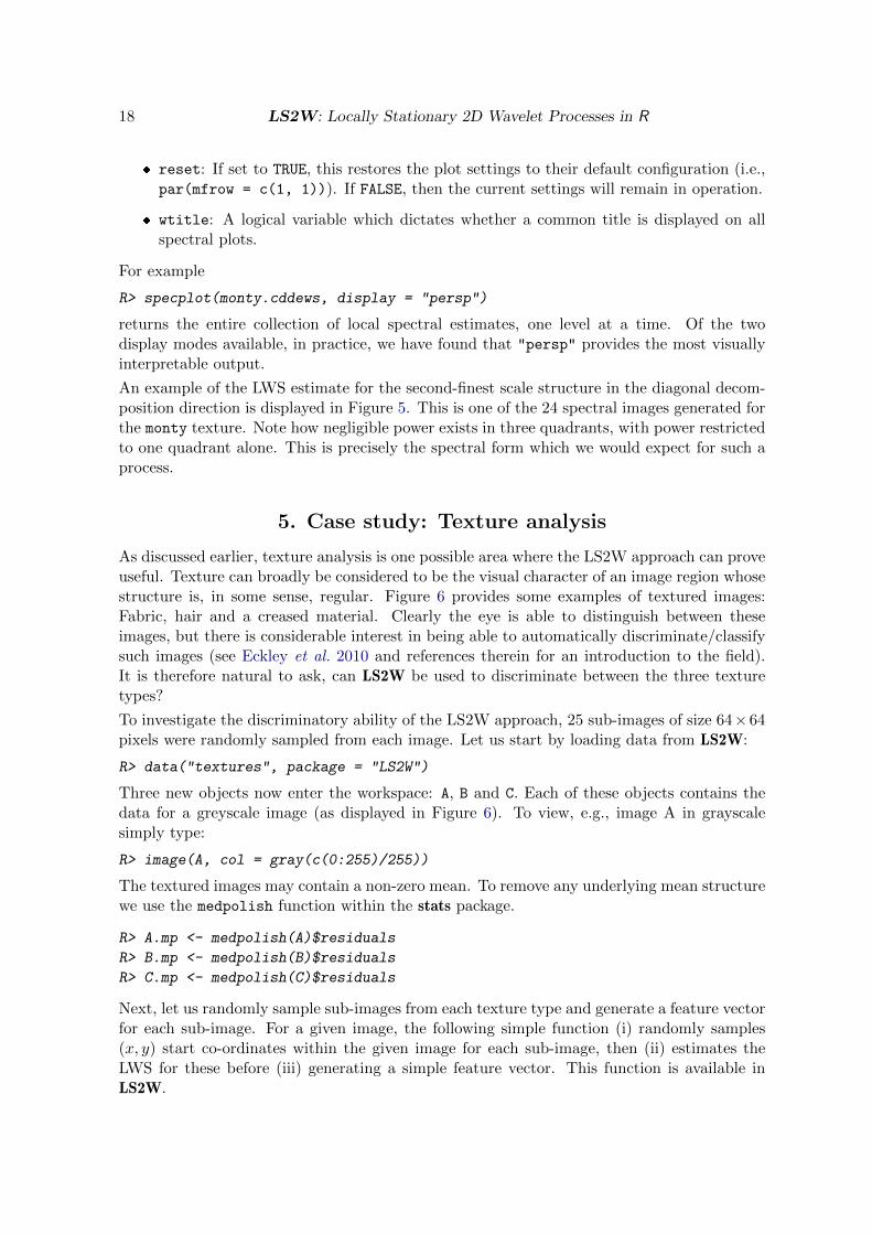
As discussed earlier, texture analysis is one possible area where the LS2W approach can proveuseful. Texture can broadly be considered to be the visual character of an image region whosestructure is, in some sense, regular. Figure 6 provides some examples of textured images:Fabric, hair and a creased material. Clearly the eye is able to distinguish between theseimages, but there is considerable interest in being able to automatically discriminate/classifysuch images (see Eckley et al. 2010 and references therein for an introduction to the field).It is therefore natural to ask, can LS2W be used to discriminate between the three texturetypes?

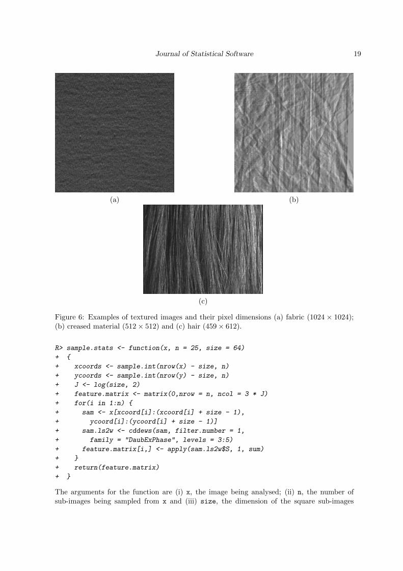
To investigate the discriminatory ability of the LS2W approach, 25 sub-images of size 64×64pixels were randomly sampled from each image. Let us start by loading data from LS2W:

R> data("textures", package = "LS2W")

Three new objects now enter the workspace: A, B and C. Each of these objects contains thedata for a greyscale image (as displayed in Figure 6). To view, e.g., image A in grayscalesimply type:

R> image(A, col = gray(c(0:255)/255))

The textured images may contain a non-zero mean. To remove any underlying mean structurewe use the medpolish function within the stats package.

R> A.mp <- medpolish(A)$residuals

R> B.mp <- medpolish(B)$residuals

R> C.mp <- medpolish(C)$residuals

Next, let us randomly sample sub-images from each texture type and generate a feature vectorfor each sub-image. For a given image, the following simple function (i) randomly samples(x, y) start co-ordinates within the given image for each sub-image, then (ii) estimates theLWS for these before (iii) generating a simple feature vector. This function is available inLS2W.


(a) (b)

(c)

Figure 6: Examples of textured images and their pixel dimensions (a) fabric (1024 × 1024);(b) creased material (512× 512) and (c) hair (459× 612).

R> sample.stats <- function(x, n = 25, size = 64)

+ {

+ xcoords <- sample.int(nrow(x) - size, n)

+ ycoords <- sample.int(nrow(y) - size, n)

+ J <- log(size, 2)

+ feature.matrix <- matrix(0,nrow = n, ncol = 3 * J)

+ for(i in 1:n) {

+ sam <- x[xcoord[i]:(xcoord[i] + size - 1),

+ ycoord[i]:(ycoord[i] + size - 1)]

+ sam.ls2w <- cddews(sam, filter.number = 1,

+ family = "DaubExPhase", levels = 3:5)

+ feature.matrix[i,] <- apply(sam.ls2w$S, 1, sum)

+ }

+ return(feature.matrix)

+ }

The arguments for the function are (i) x, the image being analysed; (ii) n, the number ofsub-images being sampled from x and (iii) size, the dimension of the square sub-images


−10 −5 0 5 10 15

−8

−6

−4

−2

02

46

First Linear Discriminant

Sec

ond

Line

ar D

iscr

imin

ant

A

A

A

A

AA

A

A

A

AAA

A

A

AA

AA

AA

A

AA

A

A

B

B

B

B

B

B

B

BB

B

BB

BB

B

BB

B

B

B

B

BB

BB

CC

C

C

C

C

C

CCCC

CCCC

C

C

C

CCC

C

CC

C

Figure 7: Linear discriminant analysis plot for texture images features derived from theLS2W model. A = fabric, B = creased material, C = hair.

sampled from x. Please note this code is available in the files which accompany this paper.When invoked, the function sample.stats returns the collection of feature vectors obtainedfor each sample obtained from the image of interest (x).

The feature vector which we adopt consists of 3J elements, each of which represents the teststatistic: t(TI) =

∑z L(z) =

∑zA−1J I([zR]). Here I denotes the smoothed (uncorrected)

local wavelet periodogram. Thus each element of the feature vector provides a measure of thecontribution made to the overall local variance structure at scale j within direction l.

To start our example, let us generate the feature vectors for 25 subsamples, each of size 64×64from images A, B and C, together with a vector of labels identifying each sample’s texture:

R> A.stats <- sample.stats(A.mp, 25, 64)

R> B.stats <- sample.stats(B.mp, 25, 64)

R> C.stats <- sample.stats(C.mp, 25, 64)

R> all.stats <- rbind(A.stats, B.stats, C.stats)

R> imlabels <- c(rep("A", 25), rep("B", 25), rep("C", 25))

As an exploratory tool to assess the potential of these LS2W-based measures, we consider adiscriminant analysis of the features using the lda function in MASS (Venables and Ripley2002). To perform this, simply invoke the following code:

R> all.stats.lda <- lda(all.stats, imlabels)

R> all.stats.ld <- predict(all.stats.lda, dimen = 2)$x


R> plot(all.stats.ld, type = "n", xlab = "First Linear Discriminant",

+ ylab = "Second Linear Discriminant")

R> text(all.stats.ld, imlabels)

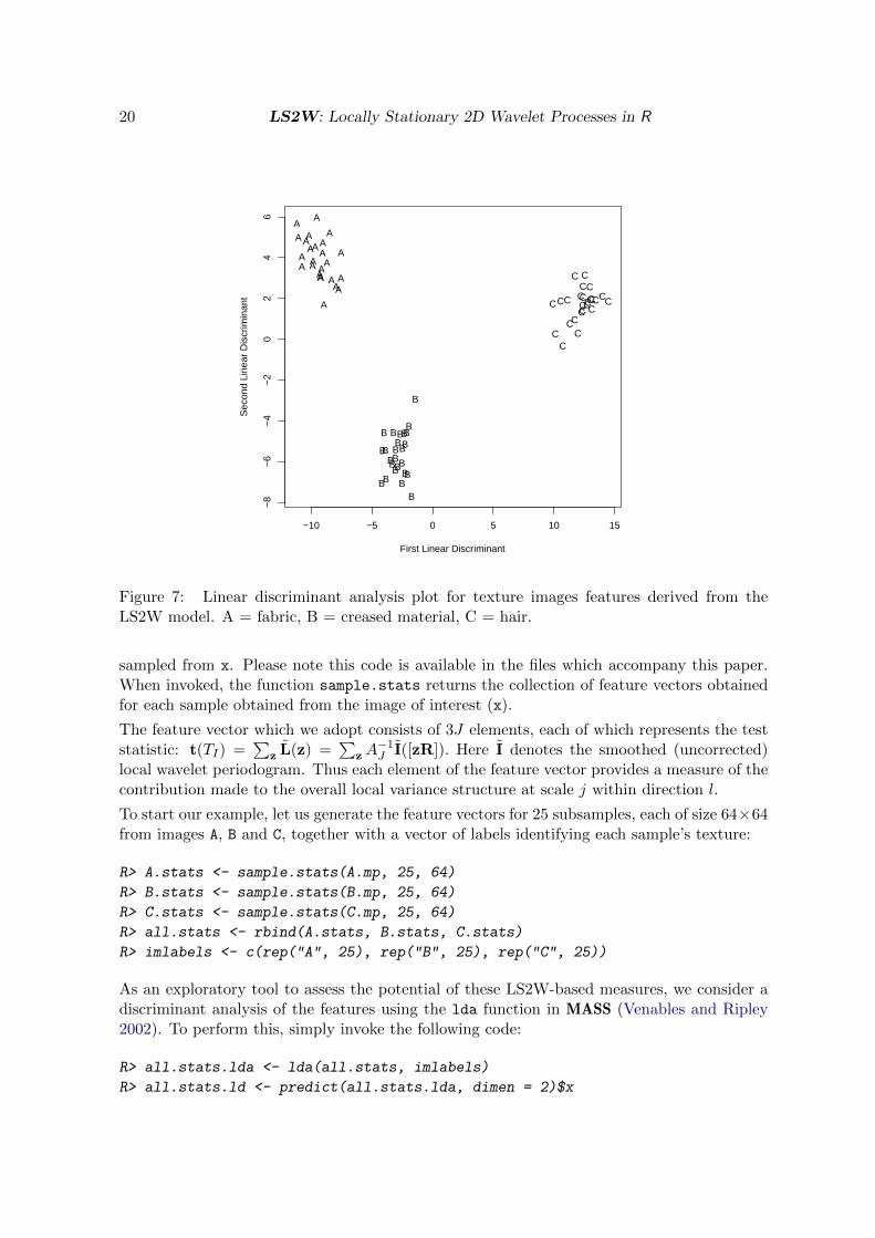
Figure 7 displays a plot of the first two linear discriminant axes for the LS2W feature set.Note in particular how one can clearly discern the three different textures. As one mightexpect, due to the regularity of the patterns in images A and B, the samples generated fromthese images fall very near one another whilst the more irregular image (C) results in morevariable samples.

6. Summary

The LS2W package provides an implementation of the LS2W estimation scheme. This is notcurrently provided by other wavelet-related R packages on CRAN. LS2W’s core functionalityconsists of the construction of two-dimensional autocorrelation wavelets, the inner productmatrix of autocorrelation wavelets and an estimation scheme for local wavelet spectra intwo-dimensions. As such LS2W is useful for estimating the (non-stationary) second-orderstructure within textured images.

Acknowledgments

The authors would like to thank Matt Nunes for his advice during the development of theLS2W package. They are also grateful to the Associate Editor and two anonymous refereesfor providing several constructive comments which have helped improve this paper. Nasonand Eckley gratefully acknowledge funding from the EPSRC SuSTaIn grant EP/D063485/1to support the work for this paper. Eckley also acknowledges the financial support of UnileverResearch.

References

Cressie NAC (1991). Statistics for Spatial Data. John Wiley & Sons.

Dahlhaus R (1997). “Fitting Time Series Models to Nonstationary Processes.” The Annals ofStatistics, 25, 1–37.

Dahlhaus R, Polonik W (2009). “Empirical Spectral Processes for Locally Stationary TimeSeries.” Bernoulli, 15, 1–39.

Daubechies I (1988). “Orthonormal Bases of Compactly Supported Wavelets.” Communica-tions on Pure and Applied Mathematics, XLI, 909–966.

Daubechies I (1992). Ten Lectures on Wavelets. SIAM, Philadelphia.

Daugman JG (1990). “An Information-Theoretic View of Analog Representation in StriateCortex.” In EL Schwartz (ed.), Computational Neuroscience, pp. 403–423. MIT Press,Cambridge.


Eckley IA (2001). Wavelet Methods for Time Series and Spatial Data. Ph.D. thesis, Universityof Bristol.

Eckley IA, Nason GP (2005). “Efficient Computation of the Inner-Product Matrix of DiscreteAutocorrelation Wavelets.” Statistics and Computing, 15, 83–92.

Eckley IA, Nason GP, Treloar RL (2010). “Locally Stationary Fields with Application to theModelling and Analysis of Image Texture.” Journal of the Royal Statistical Society C, 59,595–616.

Field DJ (1999). “Wavelets, Vision and the Statistics of Natural Scenes.” PhilosophicalTransactions of the Royal Society of London A, 357, 2527–2542.

Fryzlewicz P, Nason GP (2006). “Haar-Fisz Estimation of Evolutionary Wavelet Spectra.”Journal of the Royal Statistical Society B, 68, 611–634.

Haining RP (1978). “The Moving Average Model for Spatial Interaction.” Transactions ofthe Institute of British Geographers, 3, 202–225.

Mallat SG (1989). “A Theory for Multiresolution Signal Decomposition: The Wavelet Repre-sentation.” IEEE Transactions on Pattern Analysis and Machine Intelligence, 11, 674–693.

Mallat SG (1999). A Wavelet Tour of Signal Processing. 2nd edition. Academic Press, London.

Moore M (1988). “Spatial Linear Processes.” Communications in Statistics: Stochastic Models,4, 45–75.

Nason G (2010). “wavethresh: Wavelets Statistics and Transforms.” R package version 4.5,URL http://CRAN.R-project.org/package=wavethresh.

Nason GP (2008). Wavelet Methods in Statistics with R. Springer-Verlag.

Nason GP, Silverman BW (1995). “The Stationary Wavelet Transform and Some StatisticalApplications.” In A Antoniadis, G Oppenheim (eds.), Wavelets and Statistics, number 103in Lecture Notes in Statistics, pp. 281–300. Springer-Verlag.

Nason GP, von Sachs R, Kroisandt G (2000). “Wavelet Processes and Adaptive Estimationof the Evolutionary Wavelet Spectrum.” Journal of the Royal Statistical Society B, 62,271–292.

Priestley MB (1981). Spectral Analysis and Time Series. Academic Press, London.

R Development Core Team (2011). R: A Language and Environment for Statistical Computing.R Foundation for Statistical Computing, Vienna, Austria. ISBN 3-900051-07-0, URL http:

//www.R-project.org/.

Van Bellegem S, Dahlhaus R (2006). “Semiparametric Estimation by Model Selection forLocally Stationary Processes.” Journal of the Royal Statistical Society B, 68, 721–746.

Van Bellegem S, von Sachs R (2008). “Locally Adaptive Estimation of Evolutionary WaveletSpectra.” The Annals of Statistics, 36, 1879 – 1924.

http://CRAN.R-project.org/package=wavethresh

http://www.R-project.org/

http://www.R-project.org/


Venables WN, Ripley BD (2002). Modern Applied Statistics with S. 4th edition. Springer-Verlag, New York.

Vidakovic B (1999). Statistical Modelling by Wavelets. John Wiley & Sons.

Affiliation:

Idris A. EckleyDepartment of Mathematics and StatisticsLancaster UniversityLA1 4YF, United KingdomE-mail: [email protected]: http://www.maths.lancs.ac.uk/~eckley/

Journal of Statistical Software http://www.jstatsoft.org/

published by the American Statistical Association http://www.amstat.org/

Volume 43, Issue 3 Submitted: 2009-11-30July 2011 Accepted: 2011-06-14

mailto:[email protected]

http://www.maths.lancs.ac.uk/~eckley/

http://www.jstatsoft.org/

http://www.amstat.org/

Documents

LS2W: Implementing the Locally Stationary 2D Wavelet ... · LS2W: Implementing the Locally Stationary 2D ... in Sections3and Section4provides a tutorial ... Implementing the Locally