LRFD GEOTECHNICAL IMPLEMENTATION

Ching-Nien Tsai, P.E.

LADOTDPavement and Geotechnical Services

In Conjunction with LTRC

WHY LRFD• FHWA deadline - October 2007• LRFD is a better method

– Risk is quantified– Accounts for site and model variability– Consistent reliability– Component level risk control

• Consistent with superstructure design

LRFD vs. ASDSimilarities• Engineering principles• Engineering judgment• Capacity (resistance) evaluation• Service deformation check

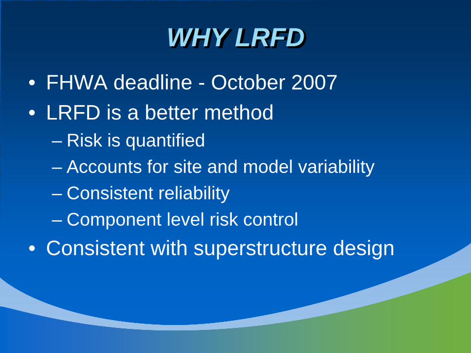
LRFD vs. ASDDifferences• Empirical vs. risk analyses• Application of resistances

– Overall safety factor vs. component level resistance factors

– Allowable resistances vs. factored resistances• Site variability and reliability of design methods• Communication among various design

professionals and construction personnel• Resource requirement

– More engineering, field investigation, lab testing and field verification tests for LRFD

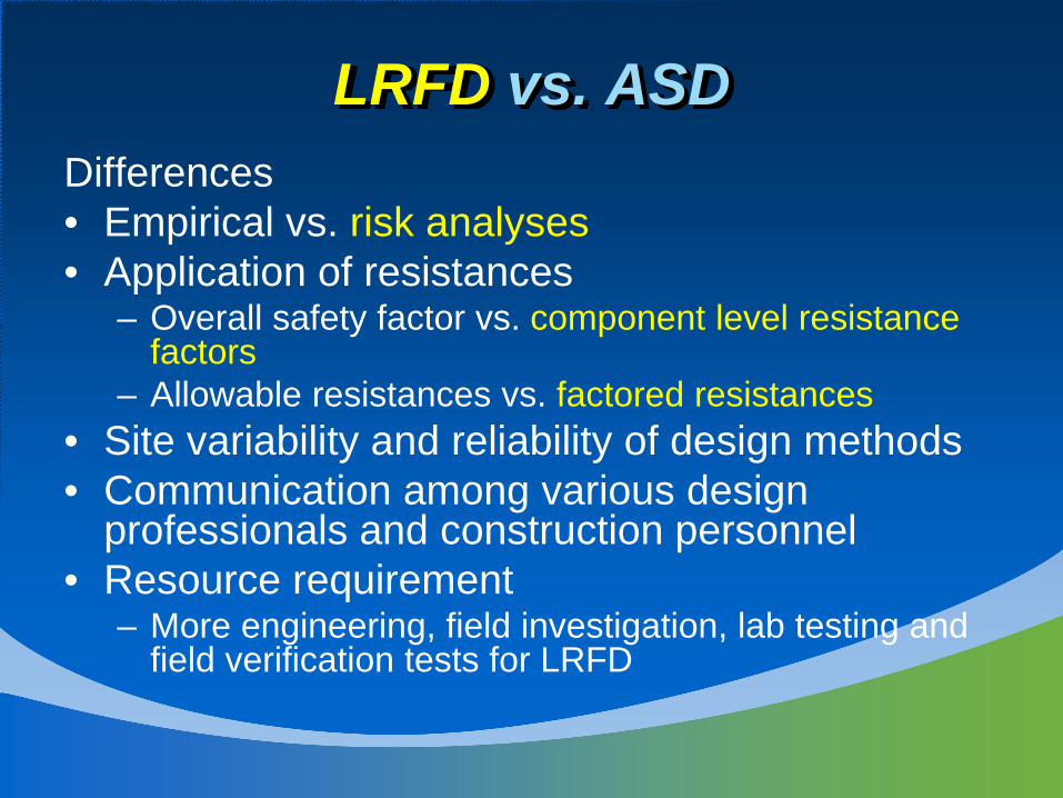
ASD VS. LRFD

∑ ∑ ≤+ FSRLLDL u /

( ) ∑∑ ∑ ≤+ uLLDL RLLDL φγγη

ASD

LRFD

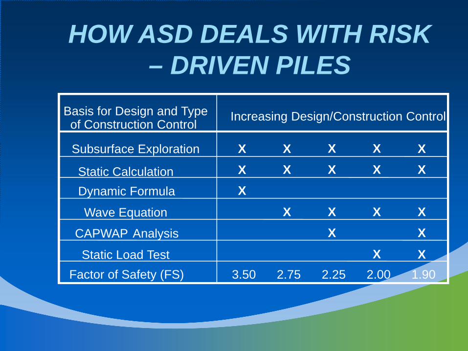
HOW ASD DEALS WITH RISK – DRIVEN PILES

Basis for Design and Typeof Construction Control Increasing Design/Construction Control

Subsurface Exploration

Static CalculationDynamic Formula

Wave Equation

CAPWAP Analysis

Static Load TestFactor of Safety (FS) 3.50

X

X

X

X

X

X

X

X

1.90

X

X

X

X

2.00

X

X

X

X

2.25

X

X

X

2.75

HOW LRFD TREATS RISK?

0

0.1

0.2

0.3

0.4

0.5

0.6

-2 -1 0 1 2 3 4 5 6

x

f(x)

iii Q∑ γη

probability of failure

Q

RnRφ

Reliability Index, β

Pf β10-1 1.2810-2 2.3310-3 3.0910-4 3.7110-5 4.2610-6 4.7510-7 5.1910-8 5.6210-9 5.99

βσg β: reliability index

0 gQR =−lnln g

Pf = shaded area

f(g) = probability density of g 2 2

R Q

g R Q

g μ μβ

σ σ σ

−= =

+

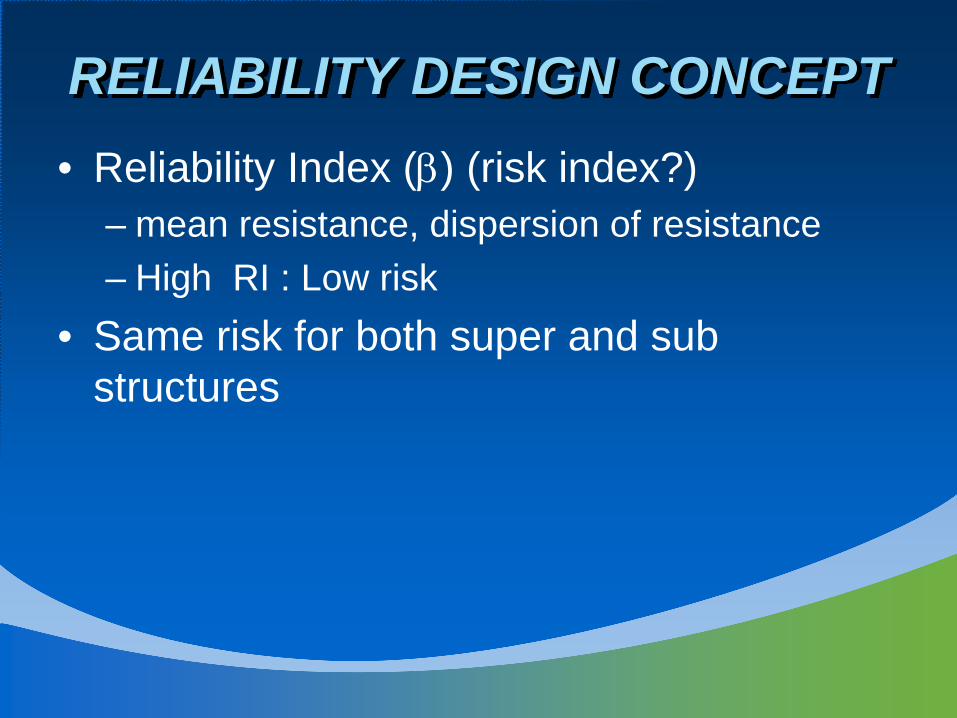
RELIABILITY DESIGN CONCEPT• Reliability Index (β) (risk index?)

– mean resistance, dispersion of resistance– High RI : Low risk

• Same risk for both super and sub structures

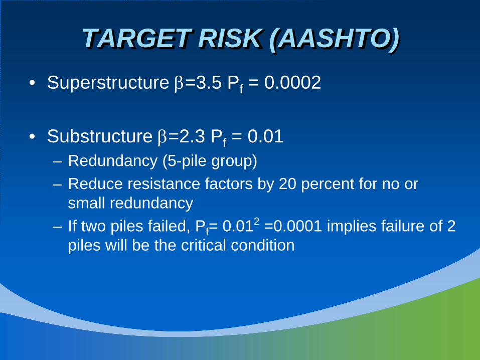
TARGET RISK (AASHTO)• Superstructure β=3.5 Pf = 0.0002

• Substructure β=2.3 Pf = 0.01– Redundancy (5-pile group)– Reduce resistance factors by 20 percent for no or

small redundancy– If two piles failed, Pf= 0.012 =0.0001 implies failure of 2

piles will be the critical condition

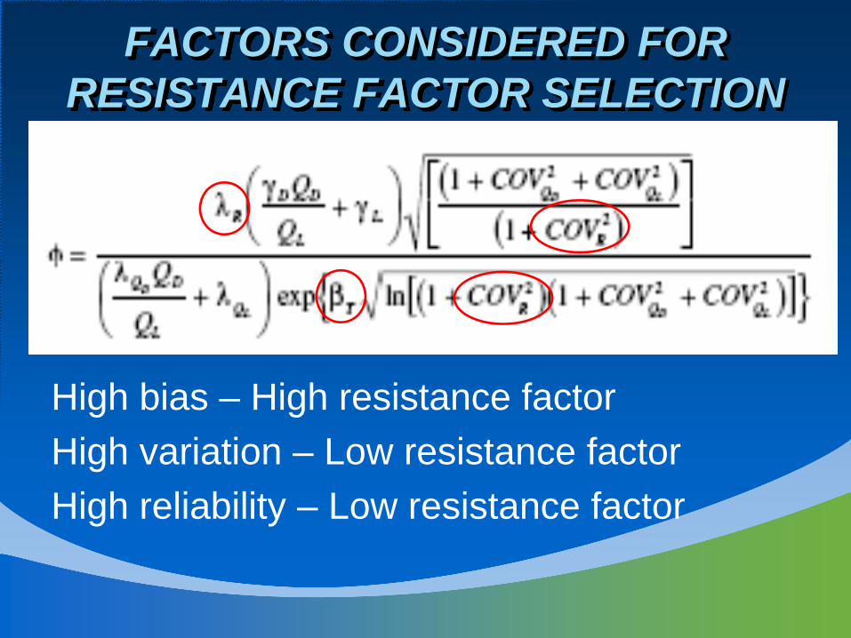
FACTORS CONSIDERED FOR RESISTANCE FACTOR SELECTION

High bias – High resistance factorHigh variation – Low resistance factorHigh reliability – Low resistance factor

AASHTO BRIDGE DESIGN SPECIFICATIONS

• Chapter 10: Foundations– 10.4 Soil and Rock Properties– 10.5 Limit States and Resistance Factors

• 10.5.5 Resistance Factors– 10.6 Spread Footings– 10.7 Driven Piles– 10.8 Drilled Shafts

• Chapter 11: Abutment, Piers and Wall

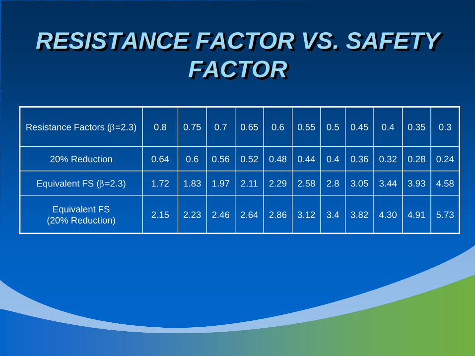
RESISTANCE FACTOR VS. SAFETY FACTOR

Resistance Factors (β=2.3) 0.8 0.75 0.7 0.65 0.6 0.55 0.5 0.45 0.4 0.35 0.3

20% Reduction 0.64 0.6 0.56 0.52 0.48 0.44 0.4 0.36 0.32 0.28 0.24

Equivalent FS (β=2.3) 1.72 1.83 1.97 2.11 2.29 2.58 2.8 3.05 3.44 3.93 4.58

Equivalent FS(20% Reduction) 2.15 2.23 2.46 2.64 2.86 3.12 3.4 3.82 4.30 4.91 5.73

FUNDAMENTALS OF LRFDPrinciples of Limit State Designs

• Four limit states• Identify the applicability of each of the

primary limit states.• Resistance

DEFINITION OF LIMIT STATE

A Limit State is a defined conditionbeyond which a structural component,

ceases to satisfy the provisions for which it is designed.

LIMIT STATES (1)• Service Limit States

– Settlements• Transient loads may be omitted for time-dependent

settlement– Horizontal Movements– Overall Stability– Scour at design flood

Service Limit State

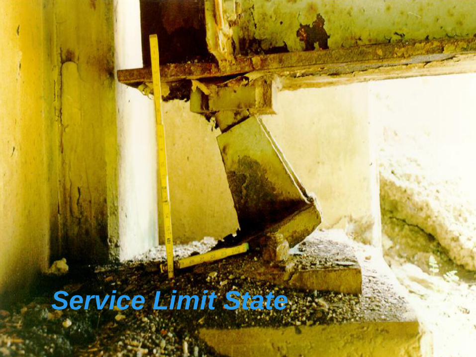
Service Limit State

LIMIT STATES (2)• Strength Limit States

– Consideration of structural resistance and loss of lateral and vertical support due to scour

• Extreme Event Limit States– Vessel collision, seismic, storm surge…– Normal resistance factors

• Fatigue Limit State

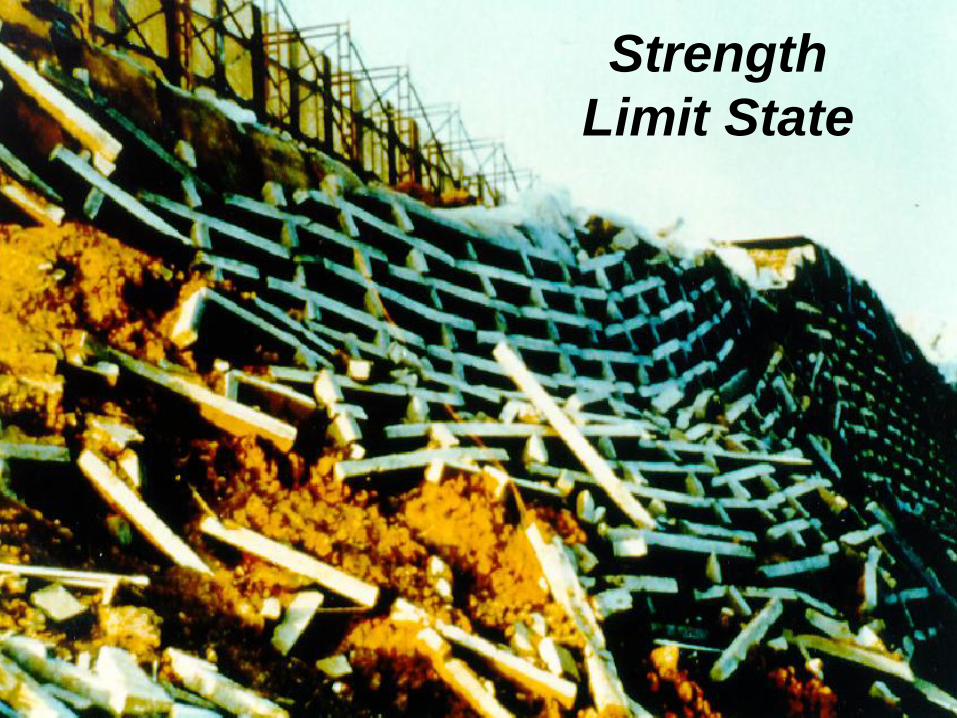
Strength Limit State

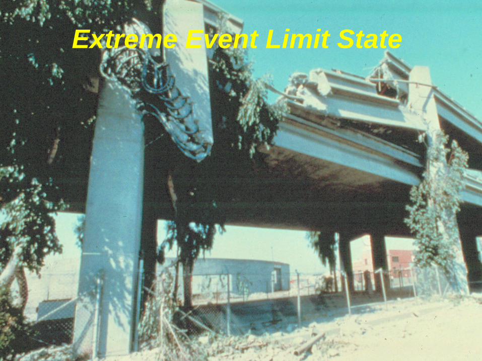
Extreme Event Limit State

DEFINITION OF RESISTANCE

Resistance is a quantifiable value that defines the point beyond which the

particular limit state under investigation for a particular component will be exceeded.

RESISTANCES

• Force (static/ dynamic, dead/ live)• Stress (normal, shear, torsional)• Number of cycles• Temperature• Strain

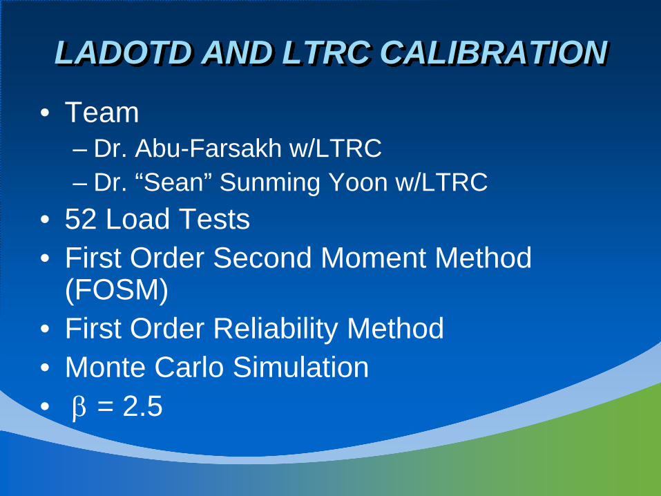
LADOTD AND LTRC CALIBRATION

• Team– Dr. Abu-Farsakh w/LTRC– Dr. “Sean” Sunming Yoon w/LTRC

• 52 Load Tests• First Order Second Moment Method

(FOSM)• First Order Reliability Method• Monte Carlo Simulation• β = 2.5

P = 1.00MR2 = 0.84

P = 1.11MR2 = 0.78

P = 0.94MR2 = 0.84

P = 1.19MR2 = 0.81

P = 1.08MR2 = 0.82

0

100

200

300

400

500

600

700

800

0 100 200 300 400 500 600 700 800

Measured Capacity (tons)

Pred

icte

d C

apac

ity (t

ons)

Static CalcCPT LCPCCPT de RuiterCPT SchermertmannCPT Average

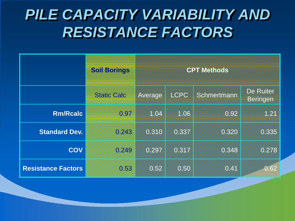
PILE CAPACITY VARIABILITY AND RESISTANCE FACTORS

Soil Borings CPT Methods

Static Calc Average LCPC Schmertmann De RuiterBeringen

Rm/Rcalc 0.97 1.04 1.06 0.92 1.21

Standard Dev. 0.243 0.310 0.337 0.320 0.335

COV 0.249 0.297 0.317 0.348 0.278

Resistance Factors 0.53 0.52 0.50 0.41 0.62

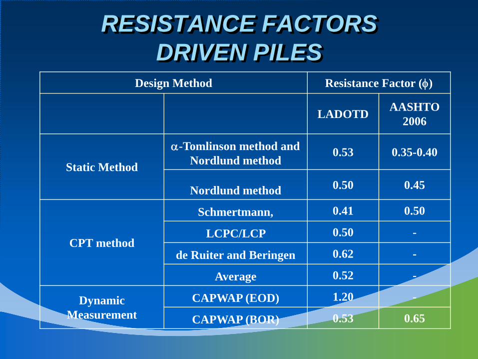
RESISTANCE FACTORSDRIVEN PILES

Design Method Resistance Factor (φ)

LADOTD AASHTO2006

Static Method

α-Tomlinson method and Nordlund method

0.53 0.35-0.40

Nordlund method 0.50 0.45

CPT method

Schmertmann, 0.41 0.50

LCPC/LCP 0.50 -

de Ruiter and Beringen 0.62 -

Average 0.52 -

Dynamic Measurement

CAPWAP (EOD) 1.20 -

CAPWAP (BOR) 0.53 0.65

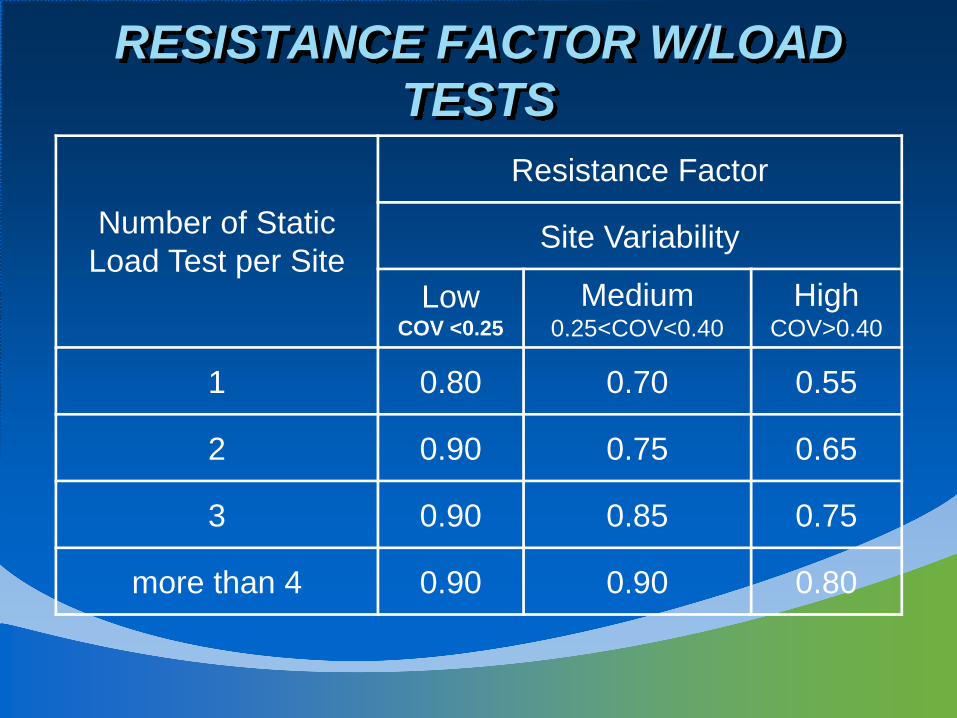
RESISTANCE FACTOR W/LOAD TESTS

Number of Static Load Test per Site

Resistance Factor

Site Variability

LowCOV <0.25

Medium0.25<COV<0.40

HighCOV>0.40

1 0.80 0.70 0.55

2 0.90 0.75 0.65

3 0.90 0.85 0.75

more than 4 0.90 0.90 0.80

0.00

0.10

0.20

0.30

0.40

0.50

0.60

0.70

0.80

0.90

1.00

0.80 0.85 0.90 0.95 1.00 1.05 1.10 1.15 1.20 1.25

Bias

Res

ista

nce

Fact

or

0.10 0.15 0.20 0.30 0.40 0.50

LOAD TEST VARIABILITY

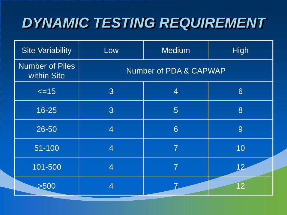
DYNAMIC TESTING REQUIREMENT

Site Variability Low Medium High

Number of Piles within Site Number of PDA & CAPWAP

<=15 3 4 6

16-25 3 5 8

26-50 4 6 9

51-100 4 7 10

101-500 4 7 12

>500 4 7 12

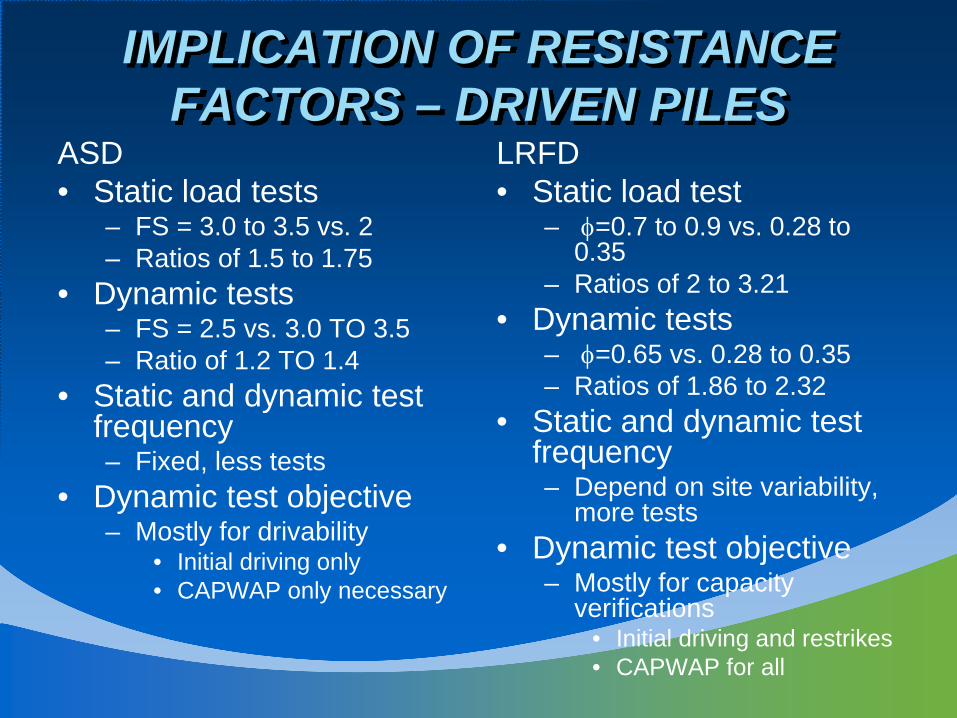
IMPLICATION OF RESISTANCE FACTORS – DRIVEN PILES

ASD• Static load tests

– FS = 3.0 to 3.5 vs. 2– Ratios of 1.5 to 1.75

• Dynamic tests– FS = 2.5 vs. 3.0 TO 3.5– Ratio of 1.2 TO 1.4

• Static and dynamic test frequency– Fixed, less tests

• Dynamic test objective– Mostly for drivability

• Initial driving only• CAPWAP only necessary

LRFD• Static load test

– φ=0.7 to 0.9 vs. 0.28 to 0.35

– Ratios of 2 to 3.21• Dynamic tests

– φ=0.65 vs. 0.28 to 0.35– Ratios of 1.86 to 2.32

• Static and dynamic test frequency– Depend on site variability,

more tests• Dynamic test objective

– Mostly for capacity verifications

• Initial driving and restrikes• CAPWAP for all

Drilled Shaft Resistance

Side Resistance

Tip Resistance

Total ResistanceA

BCD

QP

QS

QR = fQn = fqpQp + fqsQs

Displacement

Res

ista

nce

LADOTD’S CURRENT EFFORTCalibrating resistance factors for • Failure condition• 0.5 inch displacement• 1 inch displacement

AASHTO Geotechnical Resistance Factors Drilled Shafts

Method φComp φTen

α - Method (side) 0.55 0.45β - Method (side) 0.55 0.45Clay or Sand (tip) 0.5Rock (side) 0.55 0.45Rock (tip) 0.55Group (sand or clay) 0.55 0.45Load Test 0.7

AASHTO Table 10.5.5.2.3-1

DIFFICULTIES WITH DRILLED SHAFT CALIBRATION

• A lack of good load tests• Calibration is more difficult

Currently, AASHTO resistance factors are being

used until calibration is complete.

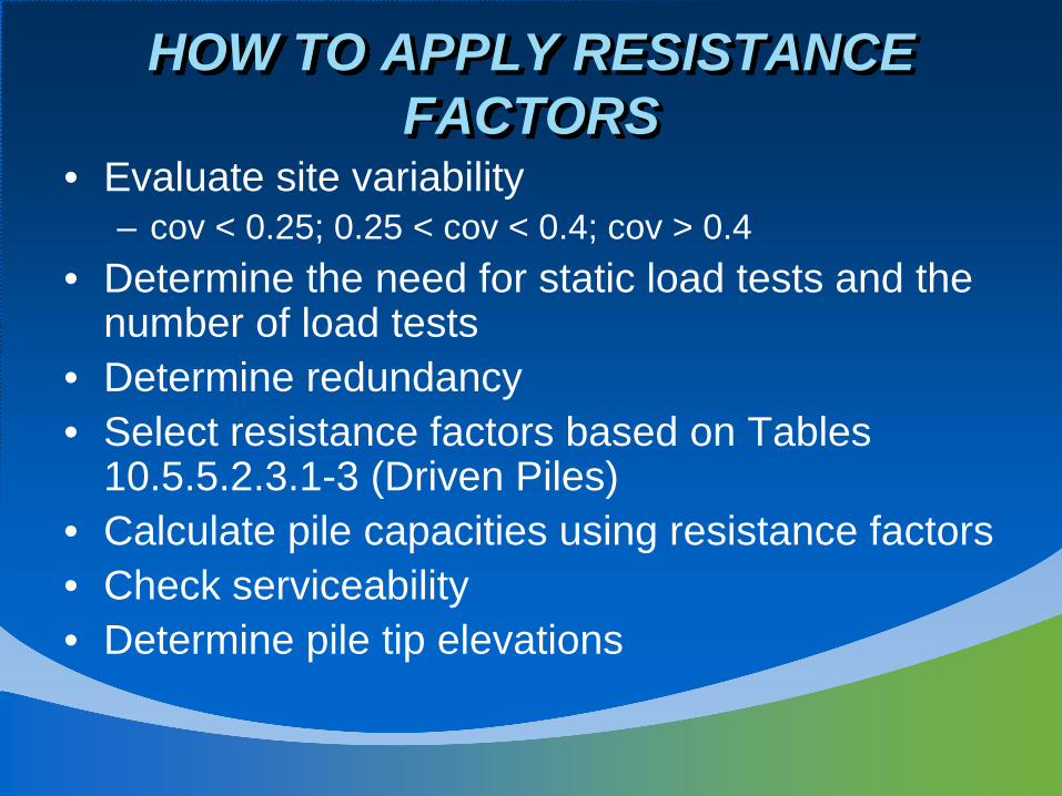
HOW TO APPLY RESISTANCE FACTORS

• Evaluate site variability– cov < 0.25; 0.25 < cov < 0.4; cov > 0.4

• Determine the need for static load tests and the number of load tests

• Determine redundancy• Select resistance factors based on Tables

10.5.5.2.3.1-3 (Driven Piles)• Calculate pile capacities using resistance factors• Check serviceability• Determine pile tip elevations

SPECIAL PROBLEMS• Downdrag• Scour• Group efficiency

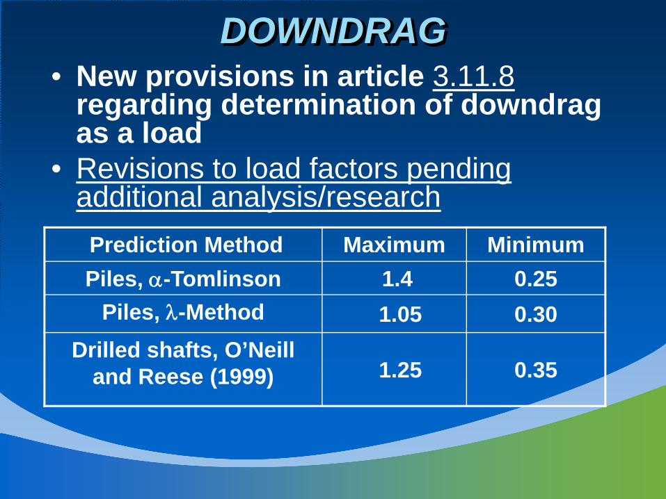
DOWNDRAG• New provisions in article 3.11.8

regarding determination of downdrag as a load

• Revisions to load factors pending additional analysis/research

Prediction Method Maximum MinimumPiles, α-Tomlinson 1.4 0.25

Piles, λ-Method 1.05 0.30Drilled shafts, O’Neill

and Reese (1999) 1.25 0.35

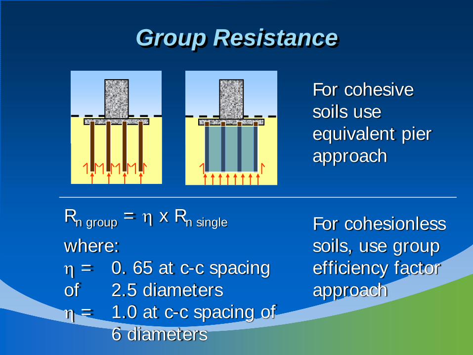
For cohesive soils use equivalent pier approach

For cohesionless soils, use group efficiency factor approach

Group Resistance

Rn group = η x Rn single

where:η = 0. 65 at c-c spacing of 2.5 diametersη = 1.0 at c-c spacing of

6 diameters

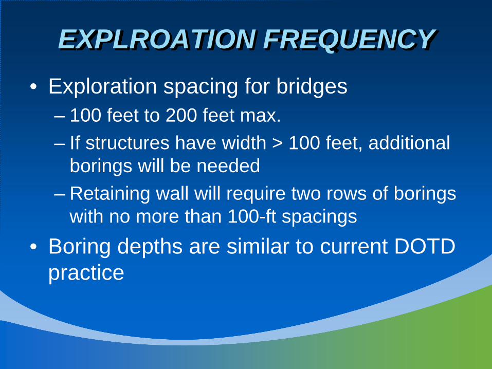
EXPLROATION FREQUENCY• Exploration spacing for bridges

– 100 feet to 200 feet max.– If structures have width > 100 feet, additional

borings will be needed– Retaining wall will require two rows of borings

with no more than 100-ft spacings • Boring depths are similar to current DOTD

practice

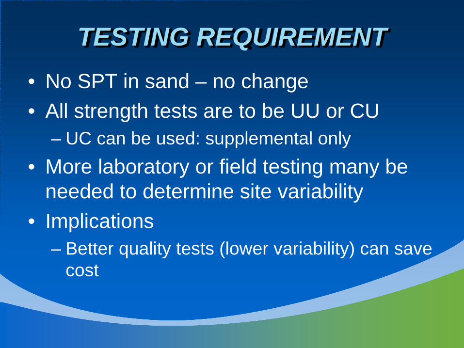
TESTING REQUIREMENT• No SPT in sand – no change• All strength tests are to be UU or CU

– UC can be used: supplemental only• More laboratory or field testing many be

needed to determine site variability• Implications

– Better quality tests (lower variability) can save cost

ENGINEERING INTERPRETATION

• Plots of depth vs. Su• Depth vs. OCR or σp’• Selection of sites (reaches) within a

project• Site variability • Selection of resistance factors

– Load tests?• Static or dynamic• quantity

– Site variability

DIFFICULTIES• Insufficient data for calibration• Slope stability• Shaft deflection calibration• Scour design compatibility

– 100 yr design; 500 yr check

FUTURE EFFORT• Continue calibration effort

– Walls and other foundation systems– Incorporate construction QC/QA into design

• Develop design manual• Modify standard specifications

– Sections 804 and 814• Training

– 2009 DOTD Conference

OTHER IMPLICATIONS• Much greater demand on resources• Feedback from construction• Methods without resistance factor

calibration cannot be used• Show justification on the resistance factor

selection• More reliable system

Questions