Embed Size (px)
Citation preview


LQR FORMATION CONTROL WITHCOLLISION AVOIDANCE OF MULTIPLE
QUADROTORS
BY
NAJIB MOHAMMED AL-ABSARI
A Thesis Presented to theDEANSHIP OF GRADUATE STUDIES
KING FAHD UNIVERSITY OF PETROLEUM & MINERALS
DHAHRAN, SAUDI ARABIA
In Partial Fulfillment of theRequirements for the degree of
MASTER OF SCIENCE
In
SYSTEMS AND CONTROL ENGINEERING
MAY 2016

KING FAHD UNIVERSITY OF PETROLEUM & MINERALS
DHAHRAN 31261, SAUDI ARABIA
DEANSHIP OF GRADUATE STUDIES
This thesis, written by NAJIB MOHAMMED AL-ABSARI under the direc-
tion of his thesis adviser and approved by his thesis committee, has been presented
to and accepted by the Dean of Graduate Studies, in partial fulfillment of the re-
quirements for the degree of MASTER OF SCIENCE IN SYSTEMS AND
CONTROL ENGINEERING.
Thesis Committee
Dr. AbdulWahid A. Al-Saif (Adviser)
Prof. Moustafa Elshafei (Member)
Dr. Sami El Ferik (Member)
Prof. Hesham K. Al-Fares
Department Chairman
Prof. Salam A. Zummo
Dean of Graduate Studies
Date

©Najib Mohammed Hasan Al-Absari2016
i

Dedicated to my elder brother Hasan Mohammed Al-Absari, who ismy support in life
ii

ACKNOWLEDGMENTS
First and Foremost, all praises are due to Allah alone Who made this possible. I
thank Him for His countless blessings and favours upon me. With His grace, all
the good deeds are completed. And Peace and Blessings of Allah upon His chosen
slave and Messenger, Muhammad, and those who follow him until the Last Day.
And then, I am quite privileged to have Dr.AbdulWahid A. Al-Saif as my advisor.
I thank him very much for his consistent support and guidance throughout this
thesis. I thank my committee members Dr.Moustafa Elshafei and Dr.Sami El
Ferik for their support and helpful inputs. I am highly indebted to Dr.Sami El
Ferik, for helping me to build the code of potential field formation in Matlab and
discussions related to it. Thanks to the Deanship of Scientific Research (DSR)
at KFUPM for their support through project number IN141048. Thanks to my
wife, kids, and my family members who have been a constant source of support.
I thank all of my friends -a quite a lot who helped me in this challenging journey.
Finally, Thanks to the Department of Systems Engineering, KFUPM for this
great opportunity and also to the Kingdom of Saudi Arabia for the numerous
endeavours they provide to students.
iii
TABLE OF CONTENTS
ACKNOWLEDGEMENT iii
LIST OF TABLES vii
LIST OF FIGURES viii
ABSTRACT (ENGLISH) xii
ABSTRACT (ARABIC) xiv
CHAPTER 1 INTRODUCTION 1
1.1 Motivation . . . . . . . . . . . . . . . . . . . . . . . . . . . . . . . 1
1.2 Thesis objectives . . . . . . . . . . . . . . . . . . . . . . . . . . . 3
CHAPTER 2 BACKGROUND AND LITERATURE REVIEW 4
2.1 Approaches of Formation Control . . . . . . . . . . . . . . . . . . 4
2.1.1 Leader–follower approach . . . . . . . . . . . . . . . . . . . 4
2.1.2 Behavioral approach . . . . . . . . . . . . . . . . . . . . . 5
2.1.3 Virtual structure approach . . . . . . . . . . . . . . . . . . 6
2.1.4 Artificial potential field techniques . . . . . . . . . . . . . 6
CHAPTER 3 PRELIMINARY 13
3.1 Quadrotor Dynamics Model . . . . . . . . . . . . . . . . . . . . . 13
3.1.1 Non-Linear Model . . . . . . . . . . . . . . . . . . . . . . 15
iv

3.1.2 Linearized Model . . . . . . . . . . . . . . . . . . . . . . . 17
3.1.3 Non-Linear Versus Linearized Model . . . . . . . . . . . . 21
CHAPTER 4 LQ CONTROL DESIGN 25
4.1 Introduction . . . . . . . . . . . . . . . . . . . . . . . . . . . . . . 25
4.2 LQ Control . . . . . . . . . . . . . . . . . . . . . . . . . . . . . . 26
4.3 simulation . . . . . . . . . . . . . . . . . . . . . . . . . . . . . . . 34
4.3.1 The Linearized model simulation . . . . . . . . . . . . . . 34
4.3.2 The non-linear model simulation . . . . . . . . . . . . . . . 35
CHAPTER 5 FORMATION FLIGHT CONTROL USING PO-
TENTIAL FIELD APPROACH 38
5.1 Leader-Follower Formation Strategy . . . . . . . . . . . . . . . . . 39
5.2 Shape Formation . . . . . . . . . . . . . . . . . . . . . . . . . . . 42
5.3 Control Design . . . . . . . . . . . . . . . . . . . . . . . . . . . . 43
5.3.1 Potential field as a 3D path generator . . . . . . . . . . . . 45
5.3.2 Potential field as a 2D path generator . . . . . . . . . . . . 49
5.4 Simulation Results . . . . . . . . . . . . . . . . . . . . . . . . . . 50
5.4.1 Flight formation with 2-D polygon . . . . . . . . . . . . . 51
5.4.2 Formation flight with 3D polygon . . . . . . . . . . . 57
CHAPTER 6 FORMATION FLIGHT CONTROL USING GEO-
METRIC APPROACH 67
6.1 Rigid Body Motion . . . . . . . . . . . . . . . . . . . . . . . . . . 68
6.2 Control Design . . . . . . . . . . . . . . . . . . . . . . . . . . . . 69
6.2.1 Collision Avoidance . . . . . . . . . . . . . . . . . . . . . . 71
6.3 SIMULATION RESULTS . . . . . . . . . . . . . . . . . . . . . . 73
6.3.1 Motion In x Direction . . . . . . . . . . . . . . . . . . . . 73
6.3.2 Motion In x − y Direction . . . . . . . . . . . . . . . . . 79
6.3.3 Motion In x − y − z Direction . . . . . . . . . . . . . . . . 79
v

6.4 Comparison . . . . . . . . . . . . . . . . . . . . . . . . . . . . . . 85
CHAPTER 7 CONCLUSION 99
7.1 Conclusion . . . . . . . . . . . . . . . . . . . . . . . . . . . . . . . 99
7.2 Future Work . . . . . . . . . . . . . . . . . . . . . . . . . . . . . . 100
REFERENCES 101
VITAE 107
vi

LIST OF TABLES
3.1 The quadrotor parameters . . . . . . . . . . . . . . . . . . . . . . 20
4.1 State-space linearization constants for quadrotor at generic opera-
tional point. . . . . . . . . . . . . . . . . . . . . . . . . . . . . . . 33
6.1 The values of Ri obtained with using the two methods. . . . . . . 97
6.2 The values of di,j obtained with using the two methods. . . . . . . 97
vii

LIST OF FIGURES
2.1 Artificial potential field [9] . . . . . . . . . . . . . . . . . . . . . . 7
3.1 Quadrotor body-fixed and inertial coordinate systems [5] . . . . . 14
3.2 Block diagram of the quadrotor dynamics [5] . . . . . . . . . . . . 15
3.3 Non-linear system dynamics . . . . . . . . . . . . . . . . . . . . . 22
3.4 Linearized system dynamics . . . . . . . . . . . . . . . . . . . . . 22
3.5 Linearised vs. non-linear system description: angular velocities . . 23
3.6 Linearised vs. non-linear system description: linear velocities . . . 23
3.7 Linear velocities errors vs. φ and θ angles . . . . . . . . . . . . . 24
3.8 Angular velocities errors vs. φ and θ angles . . . . . . . . . . . . . 24
4.1 Quadrotor’s airframe Gi,j(s) and total Hi,j(s) MIMO system. . . . 26
4.2 The linearized quadrotor with state-feedback LQ control structure 33
4.3 The non-linear quadrotor with state-feedback LQ control structure 34
4.4 Model behaviour in time along the x, y and z axes . . . . . . . . . 35
4.5 Model behaviour in space . . . . . . . . . . . . . . . . . . . . . . 36
4.6 LQ control performance on quadrotor’s non-linear model. . . . . . 37
5.1 Two followers track their leader with offsets . . . . . . . . . . . . 42
5.2 The leader with its sensing range D and two followers (Fi and Fj)
[37]. . . . . . . . . . . . . . . . . . . . . . . . . . . . . . . . . . . 43
5.3 The scheme of a follower quadrotor controlled with potential field
and LQR formation control. . . . . . . . . . . . . . . . . . . . . . 46
5.4 The group move to position 1 (different views) . . . . . . . . . . . 52
viii

5.5 The group move to position 2 (different views) . . . . . . . . . . . 53
5.6 The group move to position 3 (different views) . . . . . . . . . . . 53
5.7 The group move to position 4 (different views) . . . . . . . . . . . 54
5.8 The group move to position 5 (different views) . . . . . . . . . . . 54
5.9 The group move to position 6 (different views) . . . . . . . . . . 55
5.10 The group move to position 7 (different views) . . . . . . . . . . . 55
5.11 The group move along the full path . . . . . . . . . . . . . . . . . 56
5.12 The group move along the full path (x-y view) . . . . . . . . . . . 56
5.13 The group move along the full path in x − y direction . . . . . . . 57
5.14 The group move along the full path in x − y direction (x-y view) . 58
5.15 The group are moving to position 1 . . . . . . . . . . . . . . . . . 59
5.16 The group are moving to position 2 . . . . . . . . . . . . . . . . . 60
5.17 The group are moving to position 3 . . . . . . . . . . . . . . . . . 60
5.18 The group are moving to position 4 . . . . . . . . . . . . . . . . . 61
5.19 The group are moving to position 5 . . . . . . . . . . . . . . . . . 61
5.20 The group are moving to position 6 . . . . . . . . . . . . . . . . . 62
5.21 The group are moving to position 7 . . . . . . . . . . . . . . . . . 63
5.22 The group are navigating through the full path. . . . . . . . . . . 63
5.23 The fleet moving along the full x-y trajectory . . . . . . . . . . . 64
5.24 The fleet moving along the full x-y trajectory . . . . . . . . . . . 64
5.25 The group are moving through different positions in X-Y-Z plane 65
5.26 The group are moving through different positions in X-Y-Z plane 65
5.27 The group are moving through different positions in X-Y-Z plane 66
5.28 The group are moving through the full x-y-z trajectory . . . . . . 66
6.1 Earth fixed / inertial and body fixed frames . . . . . . . . . . . . 69
6.2 The coordinates of the leader and the ith follower in the body and
global frames . . . . . . . . . . . . . . . . . . . . . . . . . . . . . 70
6.3 The scheme of a follower quadrotor controlled with geometric for-
mation and LQR control. . . . . . . . . . . . . . . . . . . . . . . . 72
ix

6.4 The group move to the first position in a formation with θy = −30o 74
6.5 The group move to the first position in a formation with θy = −30o
(X-Y) view . . . . . . . . . . . . . . . . . . . . . . . . . . . . . . 74
6.6 The group move to the second position in a formation with θy =
−30o . . . . . . . . . . . . . . . . . . . . . . . . . . . . . . . . . 75
6.7 The group move to the second position in a formation with θy =
−30o (X-Y) view . . . . . . . . . . . . . . . . . . . . . . . . . . . 76
6.8 The group move to the third position in a formation with θy = −30o 76
6.9 The group move to the third position in a formation with θy = −30o
(X-Y) view . . . . . . . . . . . . . . . . . . . . . . . . . . . . . . 77
6.10 Moving to the fourth position in a formation with θy = −30o . . 77
6.11 The group move to the fourth position in a formation with θy =
−30o (X-Y) view . . . . . . . . . . . . . . . . . . . . . . . . . . . 78
6.12 The group move to the fifth position in a formation with θy = −30o 79
6.13 The group move to the fifth position in a formation with θy = −30o
(X-Y) view . . . . . . . . . . . . . . . . . . . . . . . . . . . . . . 80
6.14 The group move to the sixth position in a formation with θy = −30o 81
6.15 The group move to the sixth position in a formation with θy = −30o
(X-Y) view . . . . . . . . . . . . . . . . . . . . . . . . . . . . . . 81
6.16 The group move to the seventh position in a formation with θy =
−30o . . . . . . . . . . . . . . . . . . . . . . . . . . . . . . . . . 82
6.17 The group move to the seventh position in a formation with θy =
−30o (X-Y) view . . . . . . . . . . . . . . . . . . . . . . . . . . . 82
6.18 The full navigation path . . . . . . . . . . . . . . . . . . . . . . . 83
6.19 Navigating in formation with θx = 0, θy = 0 and θz = 0 . . . . . . 83
6.20 Navigating in formation with θx = −π/6, θy = −π/6 and θz = 0 . 83
6.21 Navigating in formation with θx = 0, θy = 0 and θz = π/4 . . . . 84
6.22 Navigating in x − y direction in formation with θx = 0, θy = π/6
and θz = 0 . . . . . . . . . . . . . . . . . . . . . . . . . . . . . . . 84
x
6.23 Navigating in x − y − z direction in formation with θx = 0, θy =
−π/6 and θz = 0 . . . . . . . . . . . . . . . . . . . . . . . . . . . 85
6.24 The leader reference in x direction . . . . . . . . . . . . . . . . . . 86
6.25 Achieving the desired circle radius R by agent 1 with the potential
field method . . . . . . . . . . . . . . . . . . . . . . . . . . . . . 86
6.26 Achieving the desired circle radius R by agent 1 with the geometric
method . . . . . . . . . . . . . . . . . . . . . . . . . . . . . . . . 87
6.27 Achieving the desired circle radius R by agent 2 with the potential
field method . . . . . . . . . . . . . . . . . . . . . . . . . . . . . 88
6.28 Achieving the desired circle radius R by agent 2 with the geometric
method . . . . . . . . . . . . . . . . . . . . . . . . . . . . . . . . 89
6.29 Achieving the desired circle radius R by agent 3 with the potential
field method . . . . . . . . . . . . . . . . . . . . . . . . . . . . . 90
6.30 Achieving the desired circle radius R by agent 3 with the geometric
method . . . . . . . . . . . . . . . . . . . . . . . . . . . . . . . . 91
6.31 Achieving the desired interspatial d by agents 1 and 2 with the
potential field method . . . . . . . . . . . . . . . . . . . . . . . . 92
6.32 Achieving the desired interspatial d by agents 1 and 2 with the
geometric method . . . . . . . . . . . . . . . . . . . . . . . . . . 93
6.33 Achieving the desired interspatial d by agents 1 and 3 with the
potential field method . . . . . . . . . . . . . . . . . . . . . . . . 94
6.34 Achieving the desired interspatial d by agents 1 and 3 with the
geometric method . . . . . . . . . . . . . . . . . . . . . . . . . . 95
6.35 Achieving the desired interspatial d by agents 2 and 3 with the
potential field method . . . . . . . . . . . . . . . . . . . . . . . . 96
6.36 Achieving the desired interspatial d by agents 2 and 3 with the
geometric method . . . . . . . . . . . . . . . . . . . . . . . . . . 97
xi

THESIS ABSTRACT
NAME: Najib Mohammed Al-Absari
TITLE OF STUDY: LQR FORMATION CONTROL WITH COLLISION
AVOIDANCE OF MULTIPLE QUADROTORS
MAJOR FIELD: systems and control engineering
DATE OF DEGREE: May 2016
In this thesis, two leader-follower formation control methods are proposed for
a group of quadrotors that are stabilized by using the linear quadratic regulator
(LQR) control technique. The quadrotor nonlinear model is first linearized at the
hovering operating point. Comparison between the time response of the nonlinear
model and the obtained linear one shows a good estimation with a certain range
around the operating point. Then an LQR controller is designed to stabilize the
linear model.Comparison the closed loop of both the linear and nonlinear models
is presented. The leader-follower approach is used to achieve formation control
where the position and the heading of the leader are used with offsets as references
to be tracked by the follower. To obtain shape formation, the offsets are set to
achieve the shape specifications. Two shape formation methods are used to achieve
xii

a prescribed formation flight. In the first method, the potential field technique is
used to achieve a desired formation. The attractive potential field attracts the
followers towards the leader while the repulsive potential field repulses each two
neighboring followers in order to keep a distance between them. In the second
method, the followers positions that achieve the required formation are obtained
from the geometry of the desired formation shape. These followers positions are
expressed in equations that relate them to the leader position and then given to
the followers as references to be followed. An extensive simulation is presented to
examine the validity of the results. In all simulations, a real quadrotor simulation
is used as a leader which is given a desired path as a set reference while the
followers are required to form a prescribed shape around that leader.
xiii

xiv

CHAPTER 1
INTRODUCTION
1.1 Motivation
Unmanned aerial vehicles (UAVs) have gained an extensive attention because of
their various uses in many fields. UAVs are reliable to replace manned aerial
vehicles in many areas such as military, civilian communities, and agriculture.
In military tasks, UAVs are used to carry different payloads such as radars,
cameras, and even weapons. In addition, UAVs can be used for observation and
exploring hostile environments [1].
In civilian environments, UAVs are useful for several applications such as
watching natural resources, home security, search and rescue operations, and sci-
entific research [2].
Recently, the use and control of groups of UAVs to achieve tasks cooperatively
has attracted much interest of researchers in the related fields. This is because of
the advantages that are obtained from the use of multiple vehicles instead of using
1

a more elaborated single vehicle. When comparing the task outcome of a multiple
unmanned vehicles team with that of an individual vehicle, one can realize that the
multiple vehicles overall performance can develop mission allocation, performance,
the required time, and the system safety and efficiency [3, 4].
Multi-UAV formation flight is a combination of the study of both UAV and
coordination, so it has received significant interest from both unmanned systems
and control fields. Cooperative coordination requires that a team of UAVs track
a prescribed path for flight tasks while acquiring useful information using their
on-board sensors and keeping a specified formation shape. The flight trajectory
could be a set of waypoints or a prescribed region of fly with boundaries [1].
Different approaches such as leader-follower, behavioral, and virtual structure
approaches are used to achieve formation flight. In this thesis, the leader follower
technique is used as the main method to obtain formation flight control for a group
of quadrotors. One of these vehicles is considered as a leader while the others follow
it in a prescribed formation. All the quadrotors are stabilized by using the linear
quadratic regulator (LQR) control technique. The LQR controller was designed by
linearizing the nonlinear model of the quadrotor and then applied on the nonlinear
system. The leader is set to track a reference path while the followers are set to
track the position and heading of the leader with specified offsets. By setting
these offsets, we can determine the shape formed by the group. According to the
current position of the leader and the neighboring followers, the formation control
algorithms are employed to compute the offsets and obtain the paths that navigate
2

the followers in the desired formation. To obtain a prescribed shape formation, we
use two methods to produce the followers paths. In the first method, the potential
field technique is used to achieve a desired formation. The attractive potential
field attracts the followers towards the leader while the repulsive potential field
repulses each two adjacent agents in order to keep a distance between them. In
the second method, the followers positions that achieve the required formation
are obtained from the geometry of the desired formation shape. These positions
are expressed in equations that relate them to the leader position and then given
to the followers as references to be followed. The controller will force this criteria.
1.2 Thesis objectives
This thesis introduce a new cooperative control framework in which a group of
an arbitrary number of quadrotors can achieve cooperative flight tasks. Based
on the linearized model of the quadrotor, this framework is built by combining
the LQR control technique as an inner controller with the formation algorithm
as an outer controller. The formation control algorithm is designed firstly by
using the potential field method then the potential field is replaced by a new
geometric formation method. The validity of the framework is examined based
on the quadrotor nonlinear model. The cooperative flight is achieved based on
the leader-follower approach in which the leader track a reference path while the
followers follow the leader while achieving a prescribed shape formation.
3

CHAPTER 2
BACKGROUND AND
LITERATURE REVIEW
2.1 Approaches of Formation Control
The methods of formation control are classified into three main approaches:
leader-follower, behavioral, and virtual structure approaches [5, 6, 7]. However, in
[8], the authors added the artificial potential field techniques as a fourth approach
while Chen et al. [9] combined the behavioral approach and the artificial potential
field techniques as one approach.
2.1.1 Leader–follower approach
In this technique, one of the members is selected to be the leader and the others
are nominated as followers [10]. However multiple agents can also be considered as
leaders [1]. The followers have to position themselves with respect to their leader
4
and to keep a desired position relative to the leader [3]. Control systems with the
leader-follower strategy exhibit satisfactorily good performance for flight vehicle
formations [11, 12]. Simplicity and reliability are characteristics of this method.
However, the disadvantage in this scheme is that the leader doesn’t receive an
explicit feedback from the followers [3].
The leader-follower formation control methods have been studied widely in-
cluding various methodologies like PID control approach [13], decentralized con-
trol based on Linear Quadratic Regulator (LQR) [14], nonlinear techniques, and
adaptive methods [15]-[16]. In [17] and [18], simulation comparison studies have
been done between baseline constant gain control algorithms and adaptive control
laws which adapt to the uncertainties caused by the aerodynamic interactions.
2.1.2 Behavioral approach
This approach is always combined with potential field approach in the applications
of formation control [9]. In behavioral approach, each member is assigned with
several desired behaviors and the control action is described by a weighted average
of the control that corresponds to each desired behavior for the member [5, 10].
These desired behaviors may include formation maintaining, collision avoidance,
and obstacle avoidance [6]. Mathematical analyses are difficult for behavioral
approaches and formation characteristics such as stability cannot generally be
guaranteed [10].
5

2.1.3 Virtual structure approach
In this approach, the whole formation of members is considered as a single unit.
Using the desired motion for the virtual structure, which is given, the desired
motions for the members are found [6].
In virtual structure method, three steps are needed to design the controller.
The first step is to define the desired virtual structure dynamics. The second
step is to convert the desired virtual structure motion to desired motions for each
member in the group. The last step is to design separate tracking controllers for
each member [9].
This structure is mainly used to implement sensor and manipulator systems
[10]. The advantage of this method is that formation control is uncomplicated.
The centralization, however, is a disadvantage in the virtual structure implemen-
tation and this leads to the whole system failure in the case of an agent failure
[3].
2.1.4 Artificial potential field techniques
The concept of artificial potential field based approach was explained in [13]. The
main idea of this methodology is that the vehicles move in a field of forces that
affect them. This field is similar to the electric field produced by the positive
and negative charges. The desired position is considered as an attractive charge
while obstacles are considered as repulsive charges, as shown in Figure (2.1). The
vehicle is affected by the attractive forces generated by the target and the repulsive
6

Figure 2.1: Artificial potential field [9]
forces generated by obstacles so that the motion of the vehicle could be along the
potential field gradient direction [8].
In the literature, many researches studied the quadrotors formation control
design and different proposed control methods have resulted in various perfor-
mances.
Guerrero et al [19] investigated the formation flight and trajectory following
control problems for multiple mini rotorcrafts. First, Newton-Euler formalism
was used to derive the dynamic model for a single mini rotorcraft and then the
authors used a leader/follower structure to control formation flight and designed
7

a nonlinear control bounded inputs based on separated saturations and a single
integrator consensus control for flight formation. The x and y positions for each
rotorcraft were considered as dynamical agents with full information access. The
virtual center of mass of the agents was used to achieve trajectory tracking for
the group of agents.
Mercado et al., in [20], studied the trajectory tracking and flight formation
control problem in horizontal plane for multiple unmanned aerial vehicles (UAVs)
and presented a control strategy using the leader follower scheme. They used
time scale separation of the translational and rotational quadrotor dynamics for
trajectory tracking and introduced a sliding mode controller for the translational
dynamic to provide the desired orientation for the UAV. The attitude of each is
stabilized by using a PID controller. Formation error dynamics is used by sliding
mode control law to keep formation of the follower with respect to a leader.
In [21], the authors discussed a leader-follower flocking system in which few
agents are leaders provided with knowledge on desired trajectory while the re-
maining are followers. The followers do not have global knowledge and also do
not know who the leaders are among the flocking agents, but they have the ability
to communicate their neighbors. To maintain the flocking group connected, a con-
sensus algorithm via local communication is used by all the members to estimate
the flocking center position.
In [22] Guerrero and Rogelio investigated a leader/follower type approach
based on the combination of nested saturations and a multi-agent consensus con-
8

trol to design a nonlinear controller in order to achieve flight formation for a
multiple mini rotorcraft system.
Abbas et al. [23] used two controllers to achieve formation tracking in X-Y
plane for quadrotors that are all at the same height Z. Two controllers are used
in this study. The first is a PID controller and it is used to ensure that the
leader quadrotor tracks the desired trajectory and also used by the followers to
keep formation. Then the authors used a directed lyapunov controller to achieve
quadrotors formation in X-Y plane. The artificial fish swarm algorithm has been
used to enhance the controller performance and the controller parameters have
been optimized dynamically.
Young-Cheol and Hyo-Sung [24] used a three dimensional formation controller
based on inter-agent distances. The controller is constructed from the time deriva-
tive of the Euclidean distance matrix related to the team realization.
In [25] Pilz et al. proposed a graph theory based scheme for robust distributed
controller design for formations and showed a method of making the design con-
taining performance requirements. The stability is guaranteed with the proposed
technique for all possible formations and arbitrary fast changes in the communi-
cation topology.
Turpin et al., in [26], studied formation control for a team of quadrotors where
the vehicles track a specified group trajectory with ability to change the shape
of the formation safely according to specifications. Shape vectors prescribe the
formation and command the relative separations and bearings between the quadro-
9

tors.
In [27], Lee et al. discussed the tracking control for cooperating quadrotor
unmanned aerial vehicles with a suspended load, which is considered as a point
mass connected to the quadrotors, and for an arbitrary number of vehicles. They
supposed that the point mass is linked to multiple vehicles by rigid massless
links and designed a control approach for the quadrotors to make the point mass
asymptotically tracks a desired trajectory and the quadrotors keep a prescribed
formation, with respect either to the point mass or to the inertial frame. To
avoid singularities and complexities associated with local parameterizations, a
coordinate-free fashion was used.
Eskandarpour and Majd [28] introduced an approach to achieve cooperative
formation control with obstacle and self-collisions avoidance for a group of quadro-
tors based on hierarchical model predictive control (MPC). In this study, the
control structure is divided into two layers which are lower-layer and upper-layer
control. At the lower-layer, a linear MPC was designed to stabilize quadrotors
and to accomplish trajectory tracking. Two MPC controllers were used for stabi-
lization, one of them for translational motion and the other for rotational motion.
At the upper-layer, a linear MPC controller is also designed to produce the op-
timized reference trajectory that is used by the lower-layer. To keep the vehicles
within a desired formation besides avoiding obstacles and self-collisions, three cost
functions were considered.
The authors of [29] proposed a decentralized method for formation control of
10

a team of quadrotors (UAVs). Both position and attitude of each quadrotor were
controlled by using PID controllers, which are considered as low-level controllers.
Formation control, which is considered as high-level control, was achieved by
presenting virtual springs and dampers between vehicles to generate reference
trajectories for each vehicle. Coordination and target forces are described using
spring and damping forces where springs have adaptable parameters.
Vries and Subbarao addressed a method to achieve cooperative control for
swarms of quadrotors (UAVs). First, linearized model was used to develop the
inner loop controller, which is a backstepping based controller with a nested multi-
loop structure. This controller is used to stabilize individual quadrotors and
to accomplish position tracking. Then, potential functions were used to design
cooperative controller in order to achieve the swarming behavior. Finally, obstacle
avoidance was added to the system where obstacle was modeled as a repulsive
potential function [30].
Delgado et al. [31] offered a decentralized formation control strategy for a
team of quadrotor rotorcrafts. In this work, the nested saturation control is
used to control each rotorcraft while the formation control strategy is based on
the potential field theory. Obstacle avoidance is guaranteed by using a potential
repulsive function.
In [32], Maningo introduced an alignment formation control for quadrotors
UAVs swarm of two members. The Mamdani-type of fuzzy logic control is used
to stabilize the system by equipping each vehicle with the fuzzy controller which is
11

composed of two cascaded blocks. The quadrotor’s three dimensional coordinates
and the roll, pitch, and yaw angles are used as the crisp inputs to the fuzzy
controller, while the outputs are the voltages of the motors which produce the
rotors speed. The relative positions of the quadrotors are assumed to be known,
and the roll and pitch angles are assumed to be maintained within a limited
domain to avoid vehicle overturn.
Rezaee et al. [33] proposed a leader/follower formation control of Unmanned
Aerial Vehicles (UAVs) based on fuzzy logic control. Kinematic equations were
used to design a formation strategy in order to maintain a follower at a relative
position from a leader in the body frame of the leader. Then, minimizing the
kinematic formation errors was achieved by designing fuzzy logic controllers which
control the follower speed and attitude. The UAVs dynamical models were not
considered in this work.
In [34], the problem of navigating a fleet of non-holonomic robots in a desired
leader- follower formation is investigated. The stability of the vehicles is achieved
by using the state feedback control methodology while the formation algorithm is
obtained based on the potential field strategy.
I. H. Imran, in [35] , proposed a formation control for a heterogeneous system
consists of group of non-holonomic mobile robots and one quadrotor UAV. In this
work, the Immersion and Invariance (I&I) adaptive control technique has been
used to stabilize all the vehicles, while the potential field algorithm was used to
generate the desired formation path.
12

CHAPTER 3
PRELIMINARY
This chapter describes the modeling of quadrotor UAV then linearizing the non-
linear model. It also includes a comparison between the nonlinear and linearized
models of the quadrotor. Firstly, we introduce the nonlinear model of the quadro-
tor UAV, and then use the linear approximation of the Taylor series to obtain the
linearized model around the hovering operational point. To asses its quality, the
obtained linear model is compared with the nonlinear model.
3.1 Quadrotor Dynamics Model
The quadrotor non-linear and linearized dynamic models that were derived and
identified in [36] will be used In this work. To define reference frames, two right-
handed coordinate systems were considered as shown in Figure (3.1). One of
the coordinate systems is an earth-fixed inertial frame (INF) coordinate system
while the other is a body-fixed frame. The body-fixed one has a linear velocity
13

Figure 3.1: Quadrotor body-fixed and inertial coordinate systems [5]
vector ~V = [u v w]T and an angular velocity vector ~Ω = [p q r]T . Initially the
two frames are coincident. The body-fixed frame (BFF) attitude is described by
serial rotations of its three axes about the axes of INF. Euler’s angles: φ (roll), θ
(pitch), ψ (yaw) will be used to express these rotations while the transformation
from the body-fixed frame (BFF) to the earth-fixed inertial frame (INF) will be
achieved by means of the following matrix
nb R =
cosθcosψ −cosφsinψ + sinφsinθcosψ sinφsinψ + cosφsinθcosψ
cosθsinψ cosφcosψ + sinφsinθsinψ −sinφcosψ + cosφsinθsinψ
−sinθ sinφcosθ cosφcosθ
(3.1)
As shown in Figure (3.2), the quadrotor dynamics is composed of rotor and air-
frame dynamics and the airframe dynamics contains attitude and position/altitude
dynamics.
14

Figure 3.2: Block diagram of the quadrotor dynamics [5]
3.1.1 Non-Linear Model
The quadrotor airframe non-linear model is represented by using the moment and
force equations as following, for detailed derivation see [36, 37]:
The moment equations:
p =L
Ix
3∑
i=0
γi(ωi2 − ωi
4) +IG
Ix
q4∑
j=1
ωj(−1)j +Iy − Iz
Ix
qr
q =L
Iy
3∑
i=0
γi(ωi3 − ωi
1) −IG
Iy
p4∑
j=1
ωj(−1)j +Ix − Iz
Iy
pr
r =1
Iz
4∑
j=1
(IGωj + kDω2j + Baωj)(−1)j +
Ix − Iy
Iz
pq
(3.2)
15

Due to the assumption Ix = Iy, the term Ix−Iy
Izpq will be excluded [36].
The force equations:
u = vr − wq − g sin θ
v = wp − ur + g sin φ cos θ
w = uq − vp + g cos φ cos θ −1
m
4∑
j=1
3∑
i=0
γiωij
(3.3)
where L is the lever length of each of the quadrotor arms, kD is the air drag torque
coefficient, Ba is the linear friction torque coefficient, ω is the angular speed, g
is the gravity acceleration, and Ix, Iy and Iz are aircraft’s moments of inertia
around X,Y and Z axes respectively. γi is the cubic regression coefficients which
are obtained from experimental identification for the thrust model.
For the purpose of representing the attitude dynamics in the INF we need the
Euler angles φ(t), θ(t) and ψ(t) and this can be obtained from the Euler kinematic
equations which are expressed as
φ
θ
ψ
=
1 sin φ tan θ cos φ tan θ
0 cosφ −sinφ
0sinφ
cosθ
cosφ
cosθ
p
q
r
(3.4)
16

3.1.2 Linearized Model
The linear approximation of the Taylor series is used here to obtain the linearized
quadrotor model around the operational point (p0, q0, ro), (u0, v0, w0), (φ0, θ0).
Before, however, we need to express the thrust of each rotor Tj and its deriva-
tive Tj in terms of the angular speed ωj . Although Tj (ω) can be modeled,
mathematically, as following
Tj(ω) = −kT ω2j , (3.5)
experimental tests that was conducted in [36] to identify the thrust model showed
that (3.5) does not match sufficiently accurately the obtained experimental results
and led to the following more accurate model
Tj(ω) =3∑
i=0
γiωij
= −47.7∙10−3 + 1.3∙10−3ωj − 1.44∙10−6ω2j + 5.19∙10−9ω3
j
(3.6)
and its derivative at the operational speed ωj0
Tj0 = γ1 + 2γ2ωj0 + 3γ3ω2j0
= 1.3∙10−3 + 2(−1.44∙10−6)ωj0 + 3(5.19∙10−9)ω2j0 (3.7)
To obtain the airframe linearized model, we start with linearizing the moment
17

equations.
Define
x1 = [ωj , p, q, r]T , j = 1...4
x10 = [ωj0 , p0, q0, r0]T
Δx1 = x1 − x10 = [Δωj , Δp, Δq, Δr]T
(3.8)
The linearized moment equations can be expressed as
p(x1) ≈ p0 +∂p
∂ωj
|x10Δωj +
∂p
∂p|x10
Δp +∂p
∂q|x10
Δq +∂p
∂r|x10
Δr
q(x1) ≈ q0 +∂q
∂ωj
|x10Δωj +
∂q
∂p|x10
Δp +∂q
∂q|x10
Δq +∂q
∂r|x10
Δr
r(x1) ≈ r0 +∂r
∂ωj
|x10Δωj +
∂r
∂p|x10
Δp +∂r
∂q|x10
Δq +∂r
∂r|x10
Δr
(3.9)
By applying this on (3.2), we obtain the following linearized moment equations
Δp =L
Ix
(T20Δω2 − T40Δω4) +IG
Ix
[
q0
4∑
j=1
Δωj(−1)j + Δq4∑
j=1
ωj0(−1)j
]
+Iy − Iz
Ix
(r0Δq + q0Δr)
Δq =L
Iy
(T30Δω3 − T10Δω1) −IG
Iy
[
p0
4∑
j=1
Δωj(−1)j + Δp4∑
j=1
ωj0(−1)j
]
+Ix − Iz
Iy
(p0Δr + r0Δp)
Δr =1
Iz
4∑
j=1
[IGΔωj + (2kDωj0 + Ba)Δωj ] (−1)j
(3.10)
18

The same procedure can be applied on the force and Euler kinematic equations.
Thus, we can obtain the linearized force equations as
Δu = v0Δr + r0Δv − w0Δq + q0Δw − g cos θ0Δθ
Δv = w0Δp + p0Δw − u0Δr − r0Δu + g cos φ0 cos θ0Δφ − g sin φ0 sin θ0Δθ
Δw = u0Δq + q0Δu − v0Δp − p0Δv − g sin φ0 cos θ0Δφ − g cos φ0 sin θ0Δθ −1
m
4∑
j=1
Tj0Δωj
(3.11)
and the linearized Euler kinematic equations as
Δφ = Δp + (cos φ0 tan θ0q0 − sin φ0 tan θ0r0)Δφ + (sin φ0
cos2 θ0
q0 +cos φ0
cos2 θ0
r0)Δθ
+ sin φ0 tan θ0Δq + cos φ0 tan θ0Δr
Δθ = (− sin φ0q0 − cos φ0r0)Δφ + cos φ0Δq − sin φ0Δr
Δψ = (cos φ0
cos θ0
q0 −sin φ0
cos θ0
r0)Δφ + (sin φ0 sin θ0
cos2 θ0
q0 +cos φ0 sin θ0
cos2 θ0
r0)Δθ +sin φ0
cos θ0
Δr
The above model represents only the linearized airframe dynamics. To ob-
tain the complete linearized quadrotor dynamics, the linearized rotor dynamics
is needed. For this purpose, we will use the linearized rotor dynamics with its
identified parameters obtained in [36]. This model was simplified, after applying
the Laplace transform on it, from second to first order model by discarding the
very fast pole, to become
19

Table 3.1: The quadrotor parameters
Symbol Value Description
m 0.694kg The quadrotor total massL 0.18m The lever length of each of the quadrotor armsIx 5.87∙10−3kg.m2 The moment of inertia of The quadrotor around X axesIy 5.87∙10−3kg.m2 The moment of inertia of The quadrotor around Y axesIz 10.73∙10−3kg.m2 The moment of inertia of The quadrotor around Z axes
kD 1.18∙10−7N .m.s2 Air drag torque coefficientBa 1.23∙10−6N .m.s The linear friction torque coefficientRa 260∙10−3Ω The resistance of the armaturekt 3.7∙10−3N.m/A The electric torque constantkv 7.8∙10−3V s The speed constant
IG 1.5∙10−5kg.m2 Rotor inertiaLa 1.9∙10−3H The armature impedance
Δωj(s) =Ks
s + λs
ΔUj(s)
=885, 6
s + 16.7ΔUj(s)
(3.12)
The point around which the rotor dynamics was linearized is defined by
U0 =kDRa
kt
ω20 +
BaRa + kvkt
kt
ω0 (3.13)
where U is the voltage applied to the armature of the rotor DC motor, Ra is
the resistance of the armature, kt is the electric torque constant, kv is the speed
constant [37]. Table 3.1 shows the parameters values of the quadrotor model
20

3.1.3 Non-Linear Versus Linearized Model
In this section, we repeat the comparison that have been done in [37] but in
continuous form. The quality of the linearized model is assessed by comparing it
with the non-linear model. Thus, both models have been simulated to compare
their results. a sinusoidal input is selected for the simulation as following
ω1(t) = ωhov − p ωhov sin(2πt
15)
ω2(t) = ωhov + p ωhov sin(2πt
15)
ω3(t) = ωhov
ω4(t) = ωhov
(3.14)
where
• ωhov is the required angular velocity for each rotor to maintain the quadrotor
in the hovering ,
• p is the ratio of the added sinusoidal disturbance to ωhov,
• t is the simulation time.
From figures (3.3)-(3.8), we can conclude that as long as the angles φ and θ are
less than 12 deg, the linearized model is valid to estimate the angular velocities
(p, q, r) with a maximum error of 0.1 deg/s and the linear velocities (u, v, w) with
a maximum error of 1 m/s.
21

Figure 3.3: Non-linear system dynamics
Figure 3.4: Linearized system dynamics
22

Figure 3.5: Linearised vs. non-linear system description: angular velocities
Figure 3.6: Linearised vs. non-linear system description: linear velocities
23

Figure 3.7: Linear velocities errors vs. φ and θ angles
Figure 3.8: Angular velocities errors vs. φ and θ angles
24

CHAPTER 4
LQ CONTROL DESIGN
4.1 Introduction
Quadrotor is a highly non-linear and unstable system. Thus, it needs a control
system with high efficiency and reliability. As shown in Figure (4.1), the quadrotor
system is considered as a multiple-input multiple-output (MIMO) system and
its dynamics consists of the rotor and the airframe dynamics. The fundamental
outputs shown in this structure can be manipulated to obtain all the other outputs
or states such as the position in x, y plane and the altitude h, the translational
speed ~V , and the Euler’s angles.
The control goal here is to design a control system for a single quadrotor to
track a desired position and altitude references (xref , yref , href ) on the navigation
frame. For this purpose the state-feedback LQ-optimal control is studied in the
following section.
25

Figure 4.1: Quadrotor’s airframe Gi,j(s) and total Hi,j(s) MIMO system.
4.2 LQ Control
One of the most attractive approaches of MIMO control systems is the linear
quadratic regulator (LQR or LQ). Lewis and Syrmos explained this topic in details
in [13]. The LQ is a kind of state-feedback control that is used with the state-space
description of the plant:
−→x = A~x + B~U
~y = C~x + D~U (4.1)
The LQ methodology is used to obtain the state-feedback gains matrix as following
Klqr = R−1BT S(∞) (4.2)
26

where S(∞) = S solves the Algebraic Riccti Equation(A.R.E)
0 = AT S + SA − SBR−1BT S + Q (4.3)
and this A.R.E minimizes the linear quadratic cost function (criterion)
J∞ =1
2
∫ ∞
0
(xT Qx + UT RU)dt (4.4)
with the situation of the infinite horizon.
In addition to the use of the LQ control approach for regulating the states of
the system to the state-space origin (zero), it is also used for tracking a reference.
To design a tracking controller using the LQR, artificial states are needed to be
added as the integral of the control error to guarantee asymptotic tracking. This
produces augmented A and B matrices in (4.1).
To design an LQR controller for the quadrotor system, the linearized model
of the system, explained in the previous chapter, is represented in the state-space
representation, which means that the matrices A,B,C and D have to be defined.
The system was linearized at a general operational point defined by (u0;v0;w0)∈
R3, ( φ0; θ0) ∈ R2 ∧ {θ0 6= π/2}, (p0; q0; r0) ∈ R3 and ωj0 ∈ R ∀ j = 1, ..., 4, and
the obtained complete linearized system is
27

Δp =Ia
Ix
(T20Δω2 − T40Δω4) +IG
Ix
[
q0
4∑
j=1
Δωj(−1)j + Δq4∑
j=1
ωj0(−1)j
]
+Iy − Iz
Ix
(r0Δq + q0Δr)
Δq =Ia
Iy
(T30Δω3 − T10Δω1) −IG
Iy
[
p0
4∑
j=1
Δωj(−1)j + Δp4∑
j=1
ωj0(−1)j
]
+Ix − Iz
Iy
(p0Δr + r0Δp)
Δr =1
Iz
4∑
j=1
[IGΔωj + (2kDωj0 + Ba)Δωj ] (−1)j
=1
Iz
4∑
j=1
[IGλsΔωj + (2kDωj0 + Ba)Δωj + IGksUj ] (−1)j
Δu = v0Δr + r0Δv − w0Δq + q0Δw − g cos θ0Δθ
Δv = w0Δp + p0Δw − u0Δr − r0Δu + g cos φ0 cos θ0Δφ − g sin φ0 sin θ0Δθ
Δw = u0Δq + q0Δu − v0Δp − p0Δv − g sin φ0 cos θ0Δφ − g cos φ0 sin θ0Δθ −1
m
4∑
j=1
Tj0Δωj
Δφ = Δp + (cos φ0 tan θ0q0 − sin φ0 tan θ0r0)Δφ + (sin φ0
cos2 θ0
q0 +cos φ0
cos2 θ0
r0)Δθ + sin φ0 tan θ0Δq
+ cos φ0 tan θ0Δr
Δθ = (− sin φ0q0 − cos φ0r0)Δφ + cos φ0Δq − sin φ0Δr
Δψ = (cos φ0
cos θ0
q0 −sin φ0
cos θ0
r0)Δφ + (sin φ0 sin θ0
cos2 θ0
q0 +cos φ0 sin θ0
cos2 θ0
r0)Δθ +sin φ0
cos θ0
Δr
Δω1 = λsΔω1 + ksU1
Δω2 = λsΔω2 + ksU2
Δω3 = −λsΔω3 + ksU3
Δω4 = −λsΔω4 + ksU4 (4.5)
Therefore, the vector of states x is defined as ~x = [x Δu y Δv z Δw Δφ Δp Δθ
Δq ψ Δr Δω1 Δω2 Δω3 Δω4]T and the A and B matrices can be obtained as.
28

A =
0 1 0 0 0 0 0 0 0 0 0 0 0 0 0 0
0 0 0 r0 0 −q0 0 0 au1 −ω0 0 v0 0 0 0 0
0 0 0 1 0 0 0 0 0 0 0 0 0 0 0 0
0 −r0 0 0 0 p0 av1 ω0 av2 0 0 −u0 0 0 0 0
0 0 0 0 0 1 0 0 0 0 0 0 0 0 0 0
0 q0 0 −p0 0 0 aw1 −v0 aw2 u0 0 0T10
m
T20
m
T30
m
T40
m
0 0 0 0 0 0 aφ1 + aφ4 1 aφ2 + aφ5 aφ3 0 aφ6 0 0 0 0
0 0 0 0 0 0 0 0 0 ap1 0 ap2 ap3 ap4 ap3 ap5
0 0 0 0 0 0 aθ1 + aθ3 0 0 aθ2 0 aθ4 0 0 0 0
0 0 0 0 0 0 0 aq1 0 0 0 aq2 aq3 aq4 aq5 aq4
0 0 0 0 0 0 aψ1 + aψ4 0 aψ2 + aψ5 aψ3 0 aψ6 0 0 0 0
0 0 0 0 0 0 0 0 0 0 0 0 ar1 ar2 ar3 ar4
0 0 0 0 0 0 0 0 0 0 0 0 λs 0 0 0
0 0 0 0 0 0 0 0 0 0 0 0 0 λs 0 0
0 0 0 0 0 0 0 0 0 0 0 0 0 0 −λs 0
0 0 0 0 0 0 0 0 0 0 0 0 0 0 0 −λs
(4.6)
29

B =
0 0 0 0
0 0 0 0
0 0 0 0
0 0 0 0
0 0 0 0
0 0 0 0
0 0 0 0
0 0 0 0
0 0 0 0
0 0 0 0
0 0 0 0
− IGks
Iz
IGks
Iz− IGks
Iz
IGks
Iz
ks 0 0 0
0 ks 0 0
0 0 ks 0
0 0 0 ks
(4.7)
The definition of the constants obtained from the linearization are shown in
table 4.1 [36]. As mentioned before, This is when linearizing the system around the
general operating point defined above. To linearize the system at the hovering
condition we will substitute (u0,v0,w0, φ0, θ0, p0, q0, r0, ω10 , ω20 , ω30 , ω40) by their
values at the hovering. The values of (u0,v0,w0, φ0, θ0, p0, q0, r0) at the hovering
are zeros while the values of (ω10 , ω20 , ω30 , ω40) are equal, which means ω10 =
30

ω20 = ω30 = ω40 = ωhov. At the hovering, the total thrust equals the weight of the
quadrotor. Therefore, the thrust of each rotor can be expressed as
Tj(ωhov) = mg/4
(4.8)
and, substituting from (3.6) in (4.8), we obtain
−47.7∙10−3 + 1.3∙10−3ωhov − 1.44∙10−6ω2hov + 5.19∙10−9ω3
hov − mg/4 = 0
which results in ωhov = 664.3250 rad/s.
The C and D matrices are assumed to be C =eye(16) (an identity matrix), and
D =zeros(16, 4) (a 16×4 null matrix) and all states are supposed to be directly
measured with unitary gain. In addition to the three degrees of freedom of the
quadrotor system, which are the x and y positions and the altitude h, linearizing
the system adds an extra one, which is the heading ψ (yaw angle). Hence, for
tracking control, we need to add four new states to the original (16×1) state vector
31

~x as following:
x17 = k1
∫(xref − x) dt → x17 = k1(xref − x1)
x18 = k2
∫(yref − y) dt → x18 = k2(yref
− x3)
x19 = k3
∫(zref − z) dt → x19 = k3(zref − x5)
x20 = k4
∫(ψref − ψ) dt → x20 = k4(ψref − x11)
(4.9)
where,
(xref , yref , zref ) : is the three dimensional reference position that is required to be
tracked by the quadrotor,
(x, y, z) : is the current three dimensional position of the quadrotor,
ψref : is the yaw angle reference that is required to be followed by the quadrotor,
ψ : is the current yaw angle of the quadrotor, and
k1, k2, k3, k4: are positive constants.
This will result in the augmented system shown in Figure (4.2) which has the
augmented matrices Ag and Bg. Figures (4.2) and (4.3) show the schemes of
applying the state feedback LQ control technique on both the linearized and non-
linear system models respectively.
32

Table 4.1: State-space linearization constants for quadrotor at generic operationalpoint.
ωR0 =∑4
j=1 ωj0(−1)j au1 = −g cos θ0 av1 = g cos φ0 cos θ0 av2 = −g sin φ0 sin θ0
aw1 = −g sin φ0 cos θ0 aw2 = −g cos φ0 sin θ0 aφ1 = cos φ0 tan θ0q0 aφ2 = sin φ0
cos2 θ0q0
aφ3 = sin φ0 tan θ0 aφ4 = − sin φ0 tan θ0r0 aφ5 = cos φ0
cos2 θ0r0 aφ6 = cos φ0 tan θ0
ap1 =IGωR0
+(Iy−Iz)r0
Ixap2 = (Iy−Iz)q0
Ixap3 = − IGq0
Ixap4 =
laT20+IGq0
Ix
ap5 =−laT40+IGq0
Ixaθ1 = − sin φ0q0 aθ2 = cos φ0 aθ3 = − cos φ0r0
aθ4 = − sin φ0 aq1 = −IGωR0
+(Ix−Iz)r0
Iyaq2 = − (Ix−Iz)p0
Iyaq3 =
−laT10+IGp0
Iy
aq4 = − IGp0
Iyaq5 =
laT30+IGp0
Iyaψ1 = cos φ0
cos θ0q0 aψ2 = sin φ0 sin θ0
cos2 θ0q0
aψ3 = sin φ0
cos θ0aψ4 = − sin φ0
cos θ0r0 aψ5 = cos φ0 sin θ0
cos2 θ0r0 aψ6 = cos φ0
cos θ0
arj=
IGλs−(2kDωj0+Ba)
Iz(−1)j+1 ∀j = 1...4 Tj0 = γ1 + 2γ2ωj0 + 3γ3ω
2j0 ∀j = 1...4
Figure 4.2: The linearized quadrotor with state-feedback LQ control structure
33

Figure 4.3: The non-linear quadrotor with state-feedback LQ control structure
4.3 simulation
In this section, we apply the LQR method on both the linear and nonlinear models.
4.3.1 The Linearized model simulation
When simulating the system with setting (xref , yref , zref ) = (3, 4, 5) as a reference
to be tracked by the system and letting all the states initially equal to zero, the
performance shown in Figure (4.4) is obtained.
The figure shows that the x, y and z positions asymptotically track their ref-
erences with small overshoots and settling time less than 5s. Figure (4.5) shows
the system performance in the three dimensional plane (X-Y-Z).
4.3.2 The non-linear model simulation
34
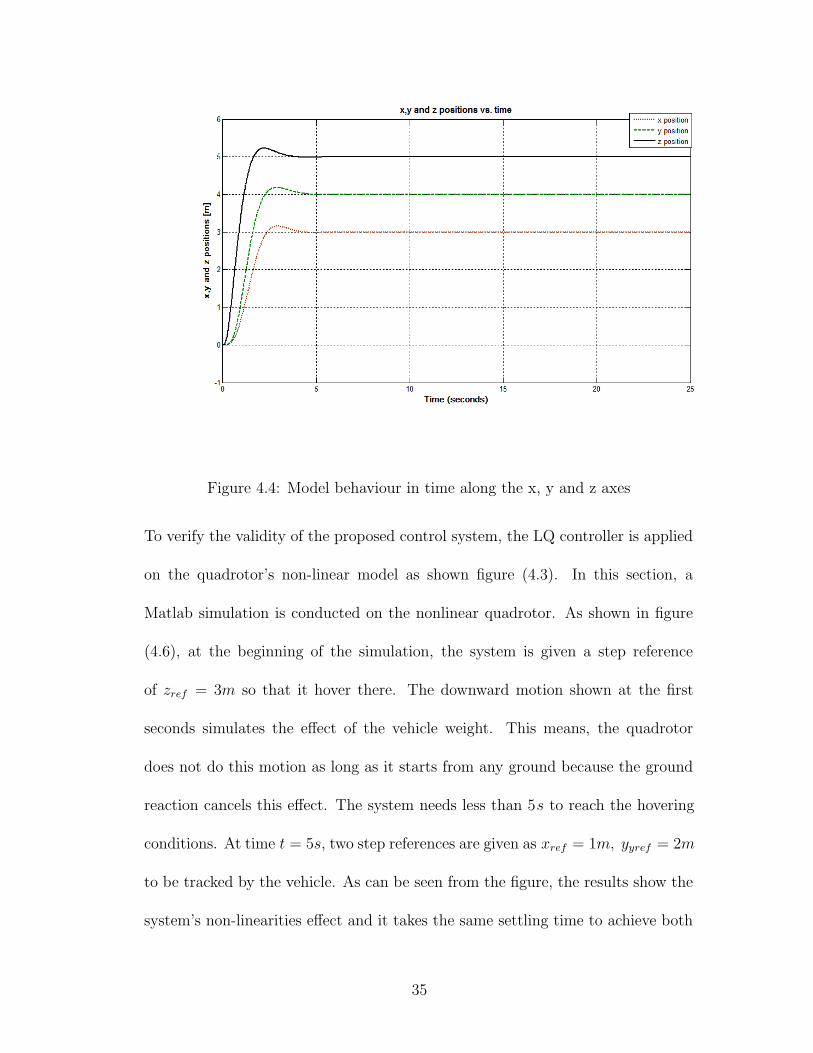
Figure 4.4: Model behaviour in time along the x, y and z axes
To verify the validity of the proposed control system, the LQ controller is applied
on the quadrotor’s non-linear model as shown figure (4.3). In this section, a
Matlab simulation is conducted on the nonlinear quadrotor. As shown in figure
(4.6), at the beginning of the simulation, the system is given a step reference
of zref = 3m so that it hover there. The downward motion shown at the first
seconds simulates the effect of the vehicle weight. This means, the quadrotor
does not do this motion as long as it starts from any ground because the ground
reaction cancels this effect. The system needs less than 5s to reach the hovering
conditions. At time t = 5s, two step references are given as xref = 1m, yyref = 2m
to be tracked by the vehicle. As can be seen from the figure, the results show the
system’s non-linearities effect and it takes the same settling time to achieve both
35

Figure 4.5: Model behaviour in space
the x and y references. The altitude z is slightly disturbed, however all states
achieve asymptotic tracking.
36

Figure 4.6: LQ control performance on quadrotor’s non-linear model.
37

CHAPTER 5
FORMATION FLIGHT
CONTROL USING
POTENTIAL FIELD
APPROACH
In this chapter, formation control using potential field technique is applied on
a group of (UAV) quadrotors that are required to navigate in a desired flight
formation. One of the group quadrotors is considered as a leader and tracks
a given reference path. The others follow the leader in a prescribed formation
shape. The potential field algorithm has two functions; one of them is attractive
function and the other is repulsive function. the attractive potential function
attracts the followers towards the leader while the repulsive function repulse each
two neighboring agents to keep interspatial distance. The methods is used under
38

the field of leader-follower formation strategy.
5.1 Leader-Follower Formation Strategy
In this formation approach, a command is given to a leader UAV to follow a
prescribed trajectory, while followers UAV track the leader with different three-
dimensional offsets with respect to the leader trajectory [37]. To obtain a desired
shape formation, the offsets are determined from the shape specifications.
Consider a group of quadrotors consists of a leader and N followers. Assuming
that all the quadrotors have the same model as the linearized model (4.1) and the
same LQR controller
−→x i = A~xi + B~Ui
~yi = C~xi + D~Ui i = 1, 2, ..., N (5.1)
~Ui = −Klqr~xi
~xi = [xi Δui yi Δvi zi Δwi Δφi Δpi Δθi Δqi ψi Δri Δω1iΔω2i
Δω3iΔω4i
]T
where ~xi ∈ Rn and ~Ui ∈ Rm are the state vector and the control input of the
quadrotor i , Klqr is the state feed back gain corresponding to LQR method.
39

To achieve Leader-Follower formation, LQR technique can be used to stabilize
all the vehicles while the reference position can be employed to obtain the desired
formation. To achieve that, the leader augmented states can be set as, (see (4.9))
xL17 = k1
∫(xref − xL) dt
xL18 = k2
∫(yref − yL) dt
xL19 = k3
∫(zref − zL) dt
xL20 = k4
∫(ψref − ψL) dt (5.2)
Since each follower have to follow the leader with a specified offset
(xiOFF, yiOFF
, ziOFF) from the leader trajectory, the augmented states for the ith
follower are
xi17 = k1
∫xL + xiOFF
− xi
xi18 = k2
∫yL + yiOFF
− yi
xi19 = k3
∫zL + ziOFF
− zi i = 1, 2, ..., N (5.3)
or
[xi17
xi18
xi19
]T = diag([k1 k2 k3]).([ xid
yid
zid
]T − [ xiy
iz
i]T ) i = 1, 2, ..., N(5.4)
[ xid
yid
zid
]T = [ xL
+ xiOFF
yL
+ yiOFF
zL + ziOFF]T (5.5)
where (xL, yL, zL) is the current three dimensional position of the leader UAV
40

in the inertial reference frame (the three-dimensional position of the leader),
(xid
yid
zid
) is the desired position in the three directions x, y, z,
(xref , yref , zref ) is the three-dimensional reference trajectory that is needed to be
tracked by the leader,
(xi, yi, zi) is the three-dimensional position of the follower i, and
(xiOFF, yiOFF
, ziOFF) is the three-dimensional offset of the follower i with re-
spect to the leader trajectory.
The heading ψi for all followers is set to track the leader’s.
xi20 =
∫ψL − ψi (5.6)
From (5.2) and (5.3) we can see that, the leader has to track the prescribed
reference trajectory while the followers have to track the output trajectory of the
leader with the offset.
Figure (5.1) shows the simulation of applying the leader-follower formation
strategy on a group of three quadrotors flying as a leader and two agents. The
leader and two agents have the same reference in z direction. However, the agents
have to follow the leader in x and y directions but with making offsets.
41

Figure 5.1: Two followers track their leader with offsets
5.2 Shape Formation
Let each quadrotor has a sensing range of D as shown in figure (5.2), and each
quadrotor has the ability to determine the positions of all its neighbors that are
located inside the sensing range. A prescribed polygon with circumcircle of radius
R is required to be tracked by the fleet quadrotors during their motion, where the
leader is located at the center while the followers are located around it. Each two
adjacent agents i, j have to be at a distant d ≤ D from each other. From the basic
geometry, R can be defined as
R =d
2 sin(π/n)
42

Figure 5.2: The leader with its sensing range D and two followers (Fi and Fj) [37].
where n represents the number of agents [34].
5.3 Control Design
The concept of cooperative control is achieved based on potential field from [35,
34]. With this technique, each follower can access the positions of the adjacent
agents in addition to the leader position. The agents’ path are obtained according
to the current positions of the leader and the neighboring followers. The attractive
and repulsive potential field concept will be applied in this work for formation
control. The desired formation is obtained by using the potential field function
to generate the paths that are needed to be tracked by the followers. To achieve
this, we need to define two potential field functions, one of them is Uatt which
attracts the followers towards the leader, and the other is Urep which keeps the
distance between each two neighboring followers as equal or greater than d. We
43

can use the following definitions to satisfy that:
Uatt =1
2katt(roi − R)2 (5.7)
Urep =
12krep(ri,j − d)2 ri,j < d
0, Otherwise
(5.8)
where:
roi : The current distance between the ith follower and the leader.
R: The desired distance between the ith follower and the leader (the circumcircle
radius of the desired polygon)
ri,j : The current distance between the ith and jth followers.
d : The desired distance between the ith and jth followers.
katt and krep : Positive constants
Then, the following associated force vector, that acts as the negative gradients
of the potential fields, will be used to control formation flight of the quadrotors
group.
F = Fo + Fij + Da (5.9)
44
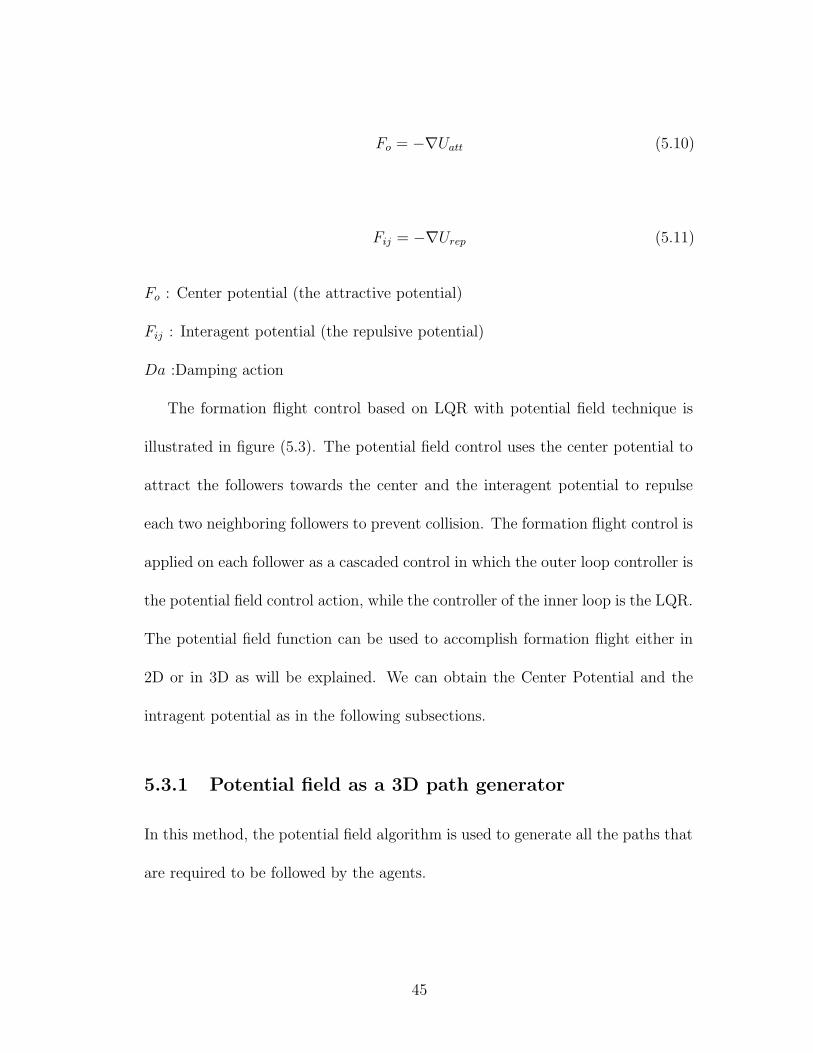
Fo = −∇Uatt (5.10)
Fij = −∇Urep (5.11)
Fo : Center potential (the attractive potential)
Fij : Interagent potential (the repulsive potential)
Da :Damping action
The formation flight control based on LQR with potential field technique is
illustrated in figure (5.3). The potential field control uses the center potential to
attract the followers towards the center and the interagent potential to repulse
each two neighboring followers to prevent collision. The formation flight control is
applied on each follower as a cascaded control in which the outer loop controller is
the potential field control action, while the controller of the inner loop is the LQR.
The potential field function can be used to accomplish formation flight either in
2D or in 3D as will be explained. We can obtain the Center Potential and the
intragent potential as in the following subsections.
5.3.1 Potential field as a 3D path generator
In this method, the potential field algorithm is used to generate all the paths that
are required to be followed by the agents.
45

Figure 5.3: The scheme of a follower quadrotor controlled with potential field andLQR formation control.
Center Potential
From (5.7) and (5.10)
Uatti =1
2katt(roi − R)2 (5.12)
Fo = −∇PiUatti(Pi)
where
Pi = [xi yi zi ψi]T
Po = [xo yo zo ψo]T
and roi can be calculated as
46

roi =√
(xi − xo)2 + ( yi − yo)2 + (zi − zo)2 + (ψi − ψo)2 (5.13)
Now by differentiating Uatti given in equation (5.12) with respect to Pi, the center
potential between the ith follower and the leader can be obtained
Fo = −
(∂Uatti
∂roi
)(∂roi
∂Pi
)
(5.14)
and(
∂Uatti
∂roi
)
= katt(roi − R) (5.15)
let
M = (xi − xo)2 + ( yi − yo)
2 + (zi − zo)2 + (ψi − ψo)
2
then
roi = M12 (5.16)
Using the chain rule, we can differentiate roi with respect to Pi as
∂roi
∂Pi
=∂roi
∂M
∂M
∂Pi
(5.17)
and from (5.16)
∂roi
∂M=
1
2M− 1
2 (5.18)
and
47

∂M
∂Pi
=
[∂M
∂xi
∂M
∂yi
∂M
∂zi
∂M
∂ψi
]T
= [2(xi − xo) 2(yi − yo) 2(zi − zo) 2(ψi − ψo)]T
= 2(Pi − Po) (5.19)
substituting (5.18) and (5.19) in (5.17) to obtain
∂roi
∂Pi
=2
2M− 1
2 (Pi − Po)
=1
roi
(Pi − Po) (5.20)
Now, substituting (5.15) and (5.20) in (5.14) results in the attractive potential as
Fo = −katt1
roi
(roi − R)(Pi(t) − Po(t)) (5.21)
Repulsive Potential
From (5.8) and (5.11)
Urepi=
12krep(ri,j − d)2 ri,j ≤ d
0, Otherwise
(5.22)
Fij = −∇PiUrep(Pi, Pj) (5.23)
48

where
Pj = [xj yj zj ψj]T
and ri,j can be calculated as
ri,j =√
(xi − xj)2 + ( yi − yj)2 + (zi − zj)2 + (ψi − ψj)2 (5.24)
Following the same steps of obtaining Fo results in the repulsive potential between
each two neighboring agents i and j as:
Fij = −krep1
ri,j
(ri,j − d) [(Pi(t) − Pj(t)) − (Pj(t) − Pi(t))] (5.25)
5.3.2 Potential field as a 2D path generator
In this method, all the quadrotors are required to achieve the desired formation
while flying in the same height. Therefore, the potential field algorithm is used
to generate the reference paths for xi, yi, and ψi while the reference path of z
position is set to be the same for all the quadrotors.
To obtain the attractive and repulsive potential, the same steps of the 3D path
generator are followed with redefining Po, Pi, and Pj as following
49

Po = [xo yo ψo]T
Pi = [xi yi ψi]T
Pj = [xj yj ψj ]T
5.4 Simulation Results
In this section we will show the results of applying the formation control using
potential field technique on a group of four quadrotors navigating in space as a
leader and three agents. As mentioned before, each quadrotor has two stages of
control. The first one is the outer stage which is responsible for formation control.
This controller produces the path that is required to be tracked by each follower.
This path is generated according to the current position of the leader and the
adjacent agents. The inner controller is the LQR controller that is responsible for
the quadrotor stability and tracking tasks. The three agents are required to form
a circle with a radius R around the leader such that the position of the leader
represents the center of the circle. Each agent has to be at a distance R from the
center and each two adjacent agents have to be at a distance d from each other.
Let R=1.5m and n=3 , then d=2R sin(pi/n)=2.598m. The leader is required to
track its reference trajectory while the followers depend on the formation control
function to produce their paths that satisfy the formation requirements. The
50

simulation is carried out firstly for the formation in the X-Y plane then for the
formation in the X-Y-Z plane. Three cases are considered. The first case is when
the leader moves in x direction, the second is when the motion is in x-y direction
and the third is when the motion is in x-y-z direction. To verify the efficiency
of the proposed control system, the control method is applied on the nonlinear
system and the following performance results have been obtained. It is clear that
the three agents are able to track the desired formation.
5.4.1 Flight formation with 2-D polygon
To obtain flight formation with a polygon in X − Y plane, the z reference for all
the group quadrotors is set to be a constant value such that they all fly at the
same height. In this case only the x and y directions are affected by the potential
field function. Two cases will be studied here; the first case is when the leader is
moving in x direction, and the second is when the leader is moving in x as well
as y direction.
Motion In x Direction
The leader and followers start from their initial hovering positions and then the
leader moves in x direction and the agents track it while keeping the desired
formation. The following figures show the performance of the LQR with potential
field formation control while navigating along a required formation path.
In figure (5.4), the leader starts moving from its initial hovering position (1,0,2)
51

Figure 5.4: The group move to position 1 (different views)
to the next position which is (2,0,2). The first follower moves from its initial posi-
tion (0.5,-1.4,2), the second follower from (0.1,1.2,2), and the third follower from
(2.5,0.2,2) respectively to form the prescribed circle around the leader. Figures
(5.5) -(5.10) show the leader navigating among different positions while the fol-
lowers track the desired formation around it. The complete navigation path for
the quadrotors group is shown in figures (5.11) and (5.12). We can see the ability
of the the LQR with potential field formation control to navigate each agent and
achieve the prescribed formation flight.
Motion In x − y Direction
In the previous simulation, the motion of the leader is set to follow a path in
x direction and here it is required to track a path in X-Y plane. This section
52

Figure 5.5: The group move to position 2 (different views)
Figure 5.6: The group move to position 3 (different views)
53

Figure 5.7: The group move to position 4 (different views)
Figure 5.8: The group move to position 5 (different views)
54
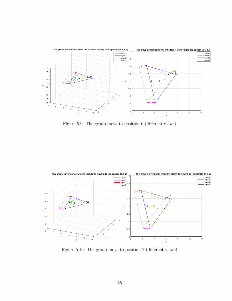
Figure 5.9: The group move to position 6 (different views)
Figure 5.10: The group move to position 7 (different views)
55

Figure 5.11: The group move along the full path
Figure 5.12: The group move along the full path (x-y view)
56
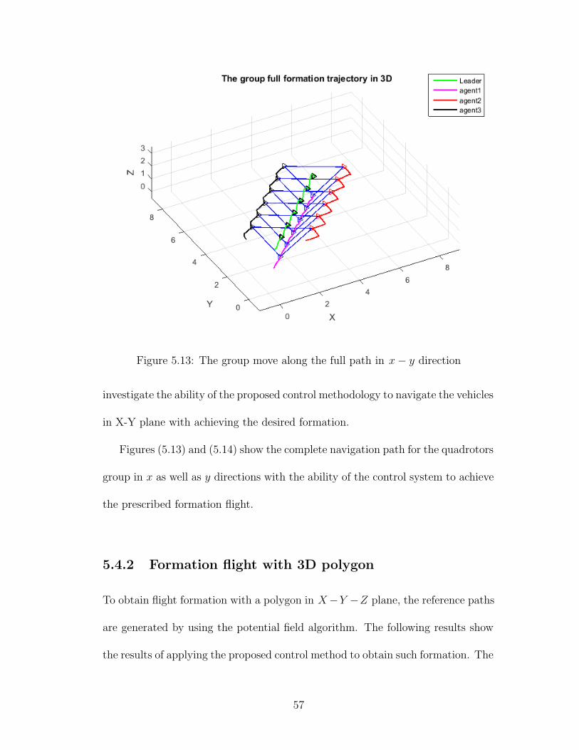
Figure 5.13: The group move along the full path in x − y direction
investigate the ability of the proposed control methodology to navigate the vehicles
in X-Y plane with achieving the desired formation.
Figures (5.13) and (5.14) show the complete navigation path for the quadrotors
group in x as well as y directions with the ability of the control system to achieve
the prescribed formation flight.
5.4.2 Formation flight with 3D polygon
To obtain flight formation with a polygon in X−Y −Z plane, the reference paths
are generated by using the potential field algorithm. The following results show
the results of applying the proposed control method to obtain such formation. The
57

Figure 5.14: The group move along the full path in x − y direction (x-y view)
58

Figure 5.15: The group are moving to position 1
figures show the ability of the control technique to achieve the task efficiently.
Motion In x Direction
In figure (5.15), the leader starts moving from its initial position (1,0,2) to the
next position which is (2,0,2). The first follower moves from its initial point
(2.2,0.8,1.8), the second follower from (-0.3,0.7,2.1), and the third follower from
(1,-1.5,1.7) respectively to form the prescribed circle around the leader. Figures
(5.16) -(5.21) show the leader navigating among different positions while the fol-
lowers track the desired formation around it. The complete navigation path for
the quadrotors group is shown in figure (5.22). We can see the ability of the the
LQR with potential field formation control to navigate each agent and achieve the
prescribed formation flight.
59

Figure 5.16: The group are moving to position 2
Figure 5.17: The group are moving to position 3
60

Figure 5.18: The group are moving to position 4
Figure 5.19: The group are moving to position 5
61

Figure 5.20: The group are moving to position 6
Motion In x − y Direction
In the previous simulation, the motion of the leader is set to follow a path in x
direction and here it is required to track a path in X-Y plane. The figures (5.23)
and (5.24) show the ability of the proposed control methodology to navigate the
vehicles in X-Y plane with achieving the desired formation.
Motion In x − y − z Direction
This section show the performance of the fleet when the leader is moving in the
three dimensional direction (x− y − z). It can be seen from figures (5.25) - (5.28)
that the LQR with potential field control system achieves the formation task
efficiently.
62

Figure 5.21: The group are moving to position 7
Figure 5.22: The group are navigating through the full path.
63

Figure 5.23: The fleet moving along the full x-y trajectory
Figure 5.24: The fleet moving along the full x-y trajectory
64

(a) The group are moving to position 1 (b) The group are moving to position 2
Figure 5.25: The group are moving through different positions in X-Y-Z plane
(a) The group are moving to position 3 (b) The group are moving to position 4
Figure 5.26: The group are moving through different positions in X-Y-Z plane
From these results it can be concluded that, the proposed control technique
works efficiently with the system nonlinear model and navigate the quadrotors
group to track the desired formation flight.
65

(a) The group are moving to position 5 (b) The group are moving to position 6
Figure 5.27: The group are moving through different positions in X-Y-Z plane
Figure 5.28: The group are moving through the full x-y-z trajectory
66

CHAPTER 6
FORMATION FLIGHT
CONTROL USING
GEOMETRIC APPROACH
In this chapter, we propose a kinematic formation method with the possibility to
select the appearance specifications for the shape that is required to be formed
by the agents. The method deals with the geometric equations that relate the
positions of the followers to the position of their leader. By considering the shape
as a rigid body, two reference frames (fixed earth/inertial and body fixed frames)
are needed to be defined. As shown in figure(6.1), The axes X − Y − Z and
x11 − y11 − z11 denote the inertial frame and the body frame of the desired shape
respectively. The roll, pitch and yaw angles: θx (roll), θy (pitch), θz (yaw) are
used to express the rotations of the shape around the global frame.
67

6.1 Rigid Body Motion
In order to determine the coordinates of a point that is located in a rigid body
moving in space, two coordinate frames are needed to be defined. The first one is a
fixed global/inertial frame n(OXY Z), while the other is a body fixed one b(oxyz).
As shown in Figure (6.1), the motion of the rigid body can be a combination of a
rotation in the global frame and a translation of the body frame origin o relative
to the origin O of the inertial frame.
If nd is a vector that indicates the position of the moving body frame origin o,
relative to the fixed global frame origin O, then the local and global coordinates
of a point P, that is attached to the rigid body, can be related by the following
equation:
nP = nb R bP + nd (6.1)
where
nP = [ nx ny nz ]
bP = [ bx by bz ]
The vector nd represents the displacement or translation of o relative to O, and nb R
is the rotation matrix that maps bP to nP when nd = 0. Equation (6.1) combines
the rotation and translation of the body frame with respect to the inertial frame.
In other words, a rigid body location can be described by the position of its frame
68

Figure 6.1: Earth fixed / inertial and body fixed frames
origin o and the orientation of the body frame, relative to the global frame [38].
6.2 Control Design
Suppose that, the quadrotors group is needed to form the circle shown in figure
(6.2). As explained in the previous section, the leader (L) is located at the circle
center while the followers are distributed around the leader to form the circle with
R radius and interspatial distance of d between each two adjacent agents.
By means of the rigid body configuration concepts, the desired positions of
the followers relative to the leader can be obtained as
[ nxfid
nyfid
nzfid]T = [ xL yL zL]T + n
b R.[ bxfid
byfid
bzfid]T (6.2)
69

Figure 6.2: The coordinates of the leader and the ith follower in the body andglobal frames
where
nb R : is the rotation matrix from the body frame to the inertial frame given as (
when the shape rotates around the inertial frame):
nb R =
cosθycosθz −cosθxsinθz + sinθxsinθycosθz sinθxsinθz + cosθxsinθycosθz
cosθysinθz cosθxcosψ + sinθxsinθysinθz −sinθxcosθz + cosθxsinθysinθz
−sinθy sinθxcosθy cosθxcosθy
If the shape rotates around its body frame, nb R will be different.
xL, yL and zL : are the coordinates of the leader position in the inertial frame.
nxfid,n yfid
and nzfid: are the desired position coordinates of the ith follower in
the inertial frame which accomplish the required formation.
bxfid,b yfid
and bzfid: are the desired position coordinates of the ith follower in the
body frame.
θfi: is the angle of the ith agent.
bxfi,b yfi
,b zfiand θfi
can be obtained geometrically from the figure as
70

bxfi= R cos θfi
byfi= R sin θfi
bzfi= 0
θfi= i ∗ 2π/n i = 1, 2, ..., n. (6.3)
where n is the number of agents.
By setting (6.2) as a reference for the ith follower, (5.4) becomes
[xfi17xfi18
xfi19]T = diag([k1 k2 k3]).([
nxfid
nyfid
nzfid]T−[ nxfi
nyfi
nzfi]T ) i = 1, 2, ..., n
(6.4)
6.2.1 Collision Avoidance
To avoid agent collision, we need to add a repulsive function that works when
the distance between any two neighboring followers becomes < d. Therefore, the
repulsive potential field in (5.23) can be used and (6.4) becomes
[xfi17xfi18
xfi19]T = diag([k1 k2 k3]).([
nxfid
nyfid
nzfid]T−[ nxfi
nyfi
nzfi]T )+Fij i = 1, 2, ..., n
(6.5)
where
71

Figure 6.3: The scheme of a follower quadrotor controlled with geometric forma-tion and LQR control.
Fij = −∇PiUrep(Pi, Pj) (6.6)
and
Urepi=
12krep(ri,j − d)2 ri,j < d
0, Otherwise
(6.7)
Then Fij can be obtained as in the pervious chapter
Fij = −krep1
ri,j
(ri,j − d) [(Pi(t) − Pj(t)) − (Pj(t) − Pi(t))] (6.8)
Figure (6.3) shows the scheme of the formation control with the geometric algo-
rithm and the LQR control approach.
72

6.3 SIMULATION RESULTS
Using the same simulation conditions that have been used with the potential field
method, the system is simulated here with the geometric method. The simulation
is carried out with three cases. The first case is when the leader moves in x
direction, the second is when the motion is in x-y direction and the third is in
x-y-z direction. With this method, we have additional specifications that can be
set to be achieved by the group of quadrotors. These specifications are the desired
shape roll - pitch - yaw angels that determine its configuration.
6.3.1 Motion In x Direction
The leader and followers start from their initial hovering positions and then the
leader moves in x direction and the agents track it while keeping the desired
formation. The following figures show the performance of the LQR with geometric
formation control while navigating along a required formation path.
Figures (6.4) and (6.5) show that the leader starts moving from its initial
hovering position (1,0,2) to the next position which is (2,0,2). The followers track
the paths obtained by the geometric functions. Therefore, the first follower moves
from its initial point (0.4,1.3,2.4), the second follower from (0.4,-1.3,2.4), and the
third follower from (2.3,0,1.3) respectively to form the prescribed circle around the
leader. Figures (6.6) -(6.17) show the leader navigating among different positions
while the followers track the desired formation around it. The complete navigation
path for the quadrotors group is shown in figure (6.18). We can see the ability
73

Figure 6.4: The group move to the first position in a formation with θy = −30o
Figure 6.5: The group move to the first position in a formation with θy = −30o
(X-Y) view
74

Figure 6.6: The group move to the second position in a formation with θy = −30o
of the the LQR with geometric formation control to navigate each agent and
achieve the prescribed formation flight with keeping a desired configuration for
the formation shape.
.
.
In figure (6.19), θx, θy and θz are set to be zeroes. The group achieved 2-D
flight formation (in X − Y plane) as shown in the figure. By setting θx = −π/6,
θy = −π/6 while keeping θz = 0, the group performance shown In figure (6.20) is
obtained. By changing θz, all the agents are shifted around the z axis of the body
frame by θz
75

Figure 6.7: The group move to the second position in a formation with θy = −30o
(X-Y) view
Figure 6.8: The group move to the third position in a formation with θy = −30o
76

Figure 6.9: The group move to the third position in a formation with θy = −30o
(X-Y) view
Figure 6.10: Moving to the fourth position in a formation with θy = −30o
77

Figure 6.11: The group move to the fourth position in a formation with θy = −30o
(X-Y) view
78

Figure 6.12: The group move to the fifth position in a formation with θy = −30o
6.3.2 Motion In x − y Direction
In this section, the leader moves in x − y direction while the followers track it in
a prescribed formation as shown in the following.
6.3.3 Motion In x − y − z Direction
Here, the control system performance is tested when the leader moves in x−y− z
direction. Figure (6.23) shows the efficiency of the formation algorithm with LQR
control to accomplish the desired formation while navigation along the complete
path.
79

Figure 6.13: The group move to the fifth position in a formation with θy = −30o
(X-Y) view
80
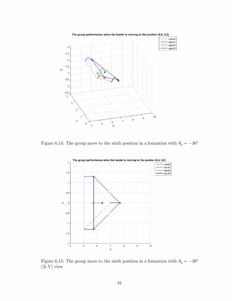
Figure 6.14: The group move to the sixth position in a formation with θy = −30o
Figure 6.15: The group move to the sixth position in a formation with θy = −30o
(X-Y) view
81

Figure 6.16: The group move to the seventh position in a formation with θy = −30o
Figure 6.17: The group move to the seventh position in a formation with θy = −30o
(X-Y) view
82
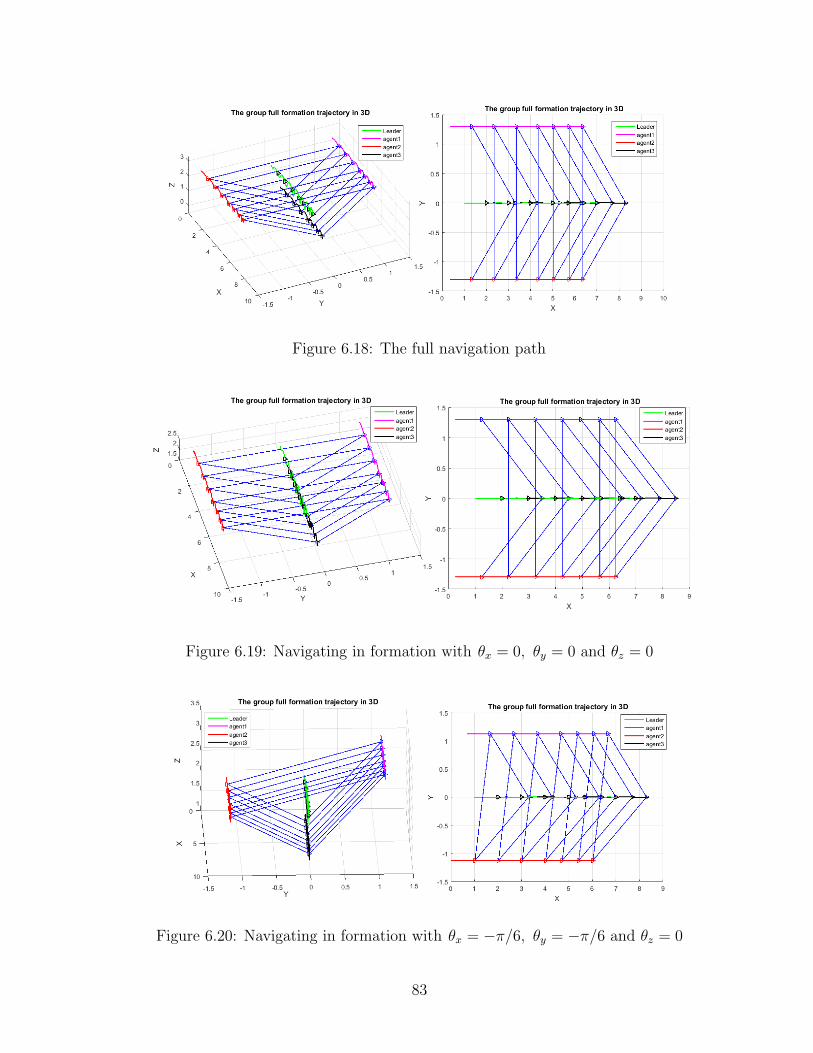
Figure 6.18: The full navigation path
Figure 6.19: Navigating in formation with θx = 0, θy = 0 and θz = 0
Figure 6.20: Navigating in formation with θx = −π/6, θy = −π/6 and θz = 0
83

Figure 6.21: Navigating in formation with θx = 0, θy = 0 and θz = π/4
Figure 6.22: Navigating in x − y direction in formation with θx = 0, θy = π/6and θz = 0
84

Figure 6.23: Navigating in x−y−z direction in formation with θx = 0, θy = −π/6and θz = 0
6.4 Comparison
To asses the performance of the proposed methods, they are compared according
to the time needed to achieve the desired formation with best accuracy. A full
formation path is set to be accomplished by the quadrotors group using the two for-
mation control methods. The time needed to achieve both the desired circle radius
R and the required interspatial distance d, is simulated for the two approaches.
R is needed to equal 1.5m. while d is needed to be d = 2Rsin(pi/3) = 2.5981m.
The leader is given its reference such that it moves in x direction with keeping its
y and z coordinates constants. Therefore, the leader reference signals are set as
(yref = 0, zref = 2m), while xref is given as shown in figure (6.24)
Figures (6.25) and (6.26) show the performance of agent 1 while positioning
85

Figure 6.24: The leader reference in x direction
Figure 6.25: Achieving the desired circle radius R by agent 1 with the potentialfield method
86

Figure 6.26: Achieving the desired circle radius R by agent 1 with the geometricmethod
87
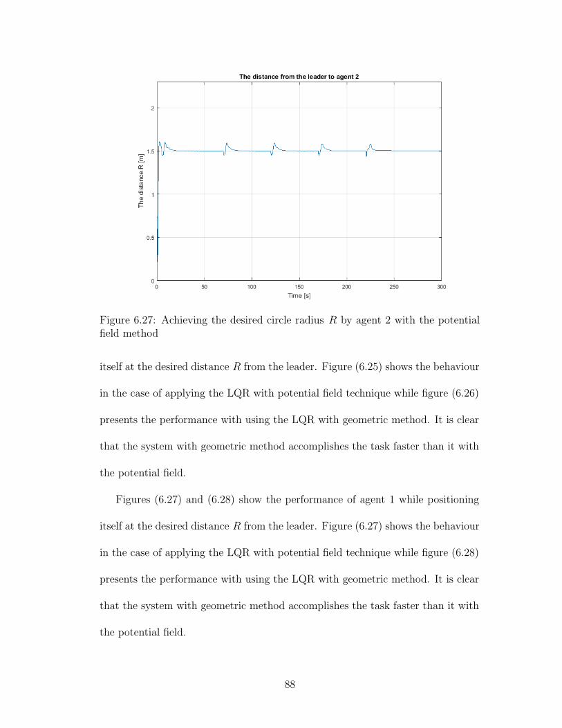
Figure 6.27: Achieving the desired circle radius R by agent 2 with the potentialfield method
itself at the desired distance R from the leader. Figure (6.25) shows the behaviour
in the case of applying the LQR with potential field technique while figure (6.26)
presents the performance with using the LQR with geometric method. It is clear
that the system with geometric method accomplishes the task faster than it with
the potential field.
Figures (6.27) and (6.28) show the performance of agent 1 while positioning
itself at the desired distance R from the leader. Figure (6.27) shows the behaviour
in the case of applying the LQR with potential field technique while figure (6.28)
presents the performance with using the LQR with geometric method. It is clear
that the system with geometric method accomplishes the task faster than it with
the potential field.
88

Figure 6.28: Achieving the desired circle radius R by agent 2 with the geometricmethod
89

Figure 6.29: Achieving the desired circle radius R by agent 3 with the potentialfield method
Figures (6.29) and (6.30) show the performance of agent 1 while positioning
itself at the desired distance R from the leader. Figure (6.29) shows the behaviour
in the case of applying the LQR with potential field technique while figure (6.30)
presents the performance with using the LQR with geometric method. It is clear
that the system with geometric method accomplishes the task faster than it with
the potential field.
Figures (6.31) and (6.32) show the performance of agents 1 and 2 while posi-
tioning themselfs at the desired distance d from each other. Figure (6.31) shows
the behaviour in the case of applying the LQR with potential field technique
while figure (6.32) presents the performance with using the LQR with geometric
method. It is clear that the system with geometric method accomplishes the task
90

Figure 6.30: Achieving the desired circle radius R by agent 3 with the geometricmethod
91

Figure 6.31: Achieving the desired interspatial d by agents 1 and 2 with thepotential field method
faster than it with the potential field.
Figures (6.33) and (6.34) show the performance of agents 1 and 3 while posi-
tioning themselves at the desired distance d from each other. Figure (6.33) shows
the behaviour in the case of applying the LQR with potential field technique
while figure (6.34) presents the performance with using the LQR with geometric
method. It is clear that the system with geometric method accomplishes the task
faster than it with the potential field.
Figures (6.35) and (6.36) show the performance of agents 2 and 3 while posi-
tioning themselves at the desired distance d from each other. Figure (6.35) shows
92

Figure 6.32: Achieving the desired interspatial d by agents 1 and 2 with thegeometric method
93

Figure 6.33: Achieving the desired interspatial d by agents 1 and 3 with thepotential field method
94

Figure 6.34: Achieving the desired interspatial d by agents 1 and 3 with thegeometric method
95

Figure 6.35: Achieving the desired interspatial d by agents 2 and 3 with thepotential field method
the behaviour in the case of applying the LQR with potential field technique
while figure (6.36) presents the performance with using the LQR with geometric
method. It is clear that the system with geometric method accomplishes the task
faster than it with the potential field.
From another side, the accuracy of positioning the followers with applying the
LQR with geometric method is more accurate than it with using the LQR with
potential field approach. we can see that in tables 6.1 and 6.2 where R i represents
the distance between the leader and the ith agent and di,j represent the distances
between the agents i and j.
From the tables, we can conclude that the system with applying the LQR
with geometric formation control approach achieve the desired positions more ac-
96
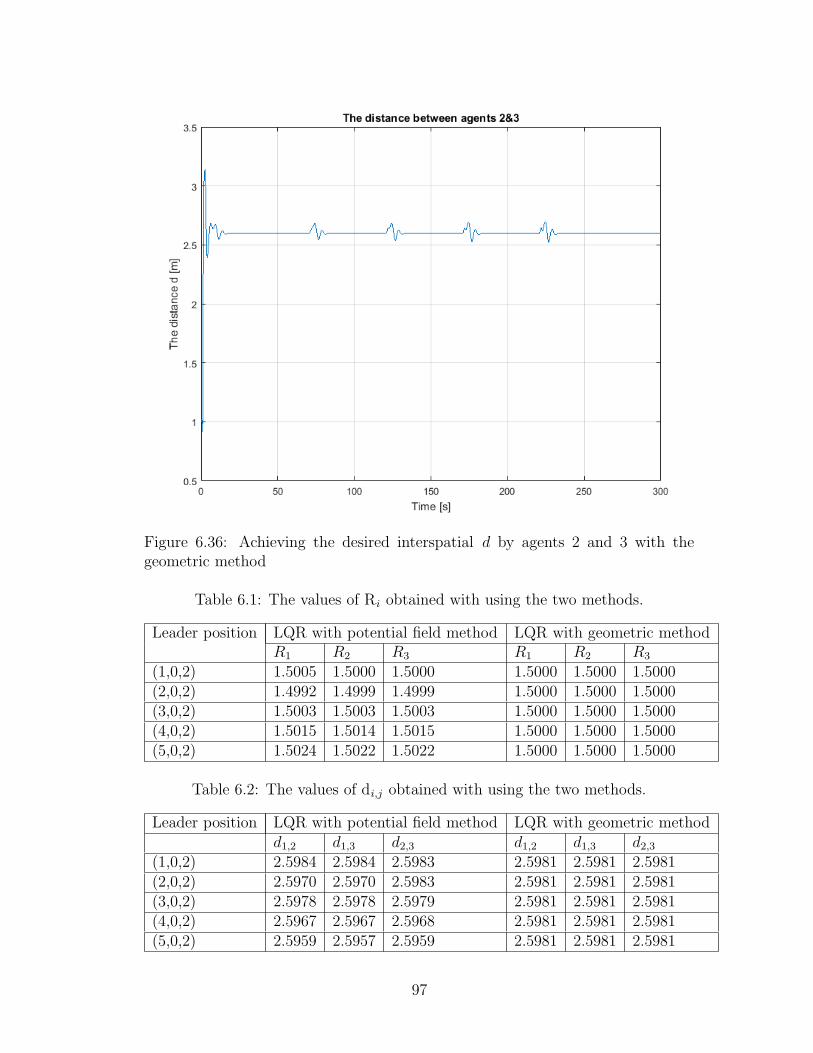
Figure 6.36: Achieving the desired interspatial d by agents 2 and 3 with thegeometric method
Table 6.1: The values of Ri obtained with using the two methods.
Leader position LQR with potential field method LQR with geometric methodR1 R2 R3 R1 R2 R3
(1,0,2) 1.5005 1.5000 1.5000 1.5000 1.5000 1.5000(2,0,2) 1.4992 1.4999 1.4999 1.5000 1.5000 1.5000(3,0,2) 1.5003 1.5003 1.5003 1.5000 1.5000 1.5000(4,0,2) 1.5015 1.5014 1.5015 1.5000 1.5000 1.5000(5,0,2) 1.5024 1.5022 1.5022 1.5000 1.5000 1.5000
Table 6.2: The values of di,j obtained with using the two methods.
Leader position LQR with potential field method LQR with geometric methodd1,2 d1,3 d2,3 d1,2 d1,3 d2,3
(1,0,2) 2.5984 2.5984 2.5983 2.5981 2.5981 2.5981(2,0,2) 2.5970 2.5970 2.5983 2.5981 2.5981 2.5981(3,0,2) 2.5978 2.5978 2.5979 2.5981 2.5981 2.5981(4,0,2) 2.5967 2.5967 2.5968 2.5981 2.5981 2.5981(5,0,2) 2.5959 2.5957 2.5959 2.5981 2.5981 2.5981
97

curately. In conclusion, In addition to the possibility of setting the configuration
of the required formation shape, the use of the LQR with geometric formation con-
trol technique provides a faster and more accurate performance for the quadrors
fleet.
98

CHAPTER 7
CONCLUSION
7.1 Conclusion
In this study, a cooperative flight control framework is designed for a fleet of
an arbitrary number of quadrotors. The LQR control technique is employed as
an inner controller that stabilize the fleet agents. Based on the leader-follower
formation approach, Two formation methodologies are used separately as an outer
controller to accomplish a desired shape formation. The LQR with potential field
technique is compared with the LQR with a geometric methodology when used
to position the fleet agents around their leader in a prescribed formation. Both
formation control methods are able to achieve the required formation. However,
the geometric method accomplish the task faster and more accurately.
99

7.2 Future Work
1. The system can be improved by using the gain scheduling technique to
obtain multiple state feedback gain.
2. The system can be addressed with the presence of communication time delay.
3. The experimental implementation for the proposed frame work is a future
study plan.
100

REFERENCES
[1] L. Di, “Cognitive formation flight in multi-unmanned aerial vehicle-based
personal remote sensing systems,” Ph.D. dissertation, Utah State University,
2011.
[2] A. J. Marasco, “Control of cooperative and collaborative team tactics in
autonomous unmanned aerial vehicles using decentralized model predictive
control,” Master’s thesis, Royal Military College of Canada, 2012.
[3] Y. Zhang and H. Mehrjerdi, “A survey on multiple unmanned vehicles for-
mation control and coordination: normal and fault situations,” in Unmanned
Aircraft Systems (ICUAS), 2013 International Conference on. IEEE, 2013,
pp. 1087–1096.
[4] B. P. Gerkey and M. J. Mataric, “A formal analysis and taxonomy of task
allocation in multi-robot systems,” The International Journal of Robotics
Research, vol. 23, no. 9, pp. 939–954, 2004.
[5] W. Ren, “Consensus seeking, formation keeping, and trajectory tracking in
multiple vehicle,” Ph.D. dissertation, Brigham Young University, 2004.
101

[6] K.-K. Oh, M.-C. Park, and H.-S. Ahn, “A survey of multi-agent formation
control,” Automatica, vol. 53, pp. 424–440, 2015.
[7] J. R. Lawton, R. W. Beard, and B. J. Young, “A decentralized approach
to formation maneuvers,” Robotics and Automation, IEEE Transactions on,
vol. 19, no. 6, pp. 933–941, 2003.
[8] X. Li, D. Zhu, and Y. Qian, “A survey on formation control algorithms for
multi-auv system,” Unmanned Systems, vol. 2, no. 04, pp. 351–359, 2014.
[9] Y. Chen and Z. Wang, “Formation control: a review and a new considera-
tion,” in Intelligent Robots and Systems, 2005.(IROS 2005). 2005 IEEE/RSJ
International Conference on. IEEE, 2005, pp. 3181–3186.
[10] S. Latyshev, “Flexible formation configuration for terrain following flight:
Formation keeping constraints,” Ph.D. dissertation, University of Southern
California, 2013.
[11] R. W. Beard, J. Lawton, F. Y. Hadaegh et al., “A coordination architecture
for spacecraft formation control,” IEEE Transactions on control systems tech-
nology, vol. 9, no. 6, pp. 777–790, 2001.
[12] G. Inalhan, D. M. Stipanovic, and C. J. Tomlin, “Decentralized optimization,
with application to multiple aircraft coordination,” in Decision and Control,
2002, Proceedings of the 41st IEEE Conference on, vol. 1. IEEE, 2002, pp.
1147–1155.
102

[13] O. Khatib, “Real-time obstacle avoidance for manipulators and mobile
robots,” The international journal of robotics research, vol. 5, no. 1, pp.
90–98, 1986.
[14] J. Wolfe, D. Chichka, and J. Speyer, “Decentralized controllers for unmanned
aerial vehicle formation flight,” AIAA paper, pp. 96–3833, 1996.
[15] C. J. Schumacher and R. Kumar, “Adaptive control of uavs in close-coupled
formation flight,” in American Control Conference, 2000. Proceedings of the
2000, vol. 2. IEEE, 2000, pp. 849–853.
[16] E. Lavretsky, N. Hovakimyan, A. Calise, and V. Stepanyan, “Adaptive vortex
seeking formation flight neurocontrol,” AIAA Paper, vol. 5726, 2003.
[17] K. Misovec, “Applied adaptive techniques for f/a-18 formation flight,” AIAA
Paper, vol. 4550, 2002.
[18] E. Lavretsky, “F/a-18 autonomous formation flight control system design,”
AIAA paper, vol. 4757, 2002.
[19] J. A. Guerrero, P. Castillo, S. Salazar, and R. Lozano, “Mini rotorcraft flight
formation control using bounded inputs,” Journal of intelligent & robotic
systems, vol. 65, no. 1-4, pp. 175–186, 2012.
[20] D. Mercado, R. Castro, and R. Lozano, “Quadrotors flight formation con-
trol using a leader-follower approach,” in Proceedings of the 2103 European
Control Conference (ECC), Zurich, Switzerland, 2013, pp. 3858–3863.
103

[21] Z. Wang and D. Gu, “A leader-follower flocking system based on estimated
flocking center,” in Robot Intelligence. Springer, 2010, pp. 191–208.
[22] J. Guerrero and R. Lozano, “Flight formation of multiple mini rotorcraft
based on nested saturations,” in Intelligent Robots and Systems (IROS), 2010
IEEE/RSJ International Conference on. IEEE, 2010, pp. 634–639.
[23] R. Abbas and Q. Wu, “Improved leader follower formation controller for
multiple quadrotors based afsa,” TELKOMNIKA (Telecommunication Com-
puting Electronics and Control), vol. 13, no. 1, pp. 85–92, 2015.
[24] Y.-C. Choi and H.-S. Ahn, “Formation control of quad-rotors in three dimen-
sion based on euclidean distance dynamics matrix,” in Control, Automation
and Systems (ICCAS), 2011 11th International Conference on. IEEE, 2011,
pp. 1168–1173.
[25] U. Pilz, A. P. Popov, and H. Werner, “Robust controller design for formation
flight of quad-rotor helicopters.” in CDC, 2009, pp. 8322–8327.
[26] M. Turpin, N. Michael, and V. Kumar, “Decentralized formation control with
variable shapes for aerial robots,” in Robotics and Automation (ICRA), 2012
IEEE International Conference on. IEEE, 2012, pp. 23–30.
[27] T. Lee, K. Sreenath, and V. Kumar, “Geometric control of cooperating mul-
tiple quadrotor uavs with a suspended payload,” in Decision and Control
(CDC), 2013 IEEE 52nd Annual Conference on. IEEE, 2013, pp. 5510–
5515.
104

[28] A. Eskandarpour and V. J. Majd, “Cooperative formation control of quadro-
tors with obstacle avoidance and self collisions based on a hierarchical mpc
approach,” in Robotics and Mechatronics (ICRoM), 2014 Second RSI/ISM
International Conference on. IEEE, 2014, pp. 351–356.
[29] M. A. Guney and M. Unel, “Formation control of a group of micro aerial
vehicles (mavs),” in Systems, Man, and Cybernetics (SMC), 2013 IEEE In-
ternational Conference on. IEEE, 2013, pp. 929–934.
[30] E. De Vries and K. Subbarao, Cooperative control of swarms of unmanned
aerial vehicles. American Institute of Aeronautics and Astronautics (AIAA),
2011.
[31] L. A. G. Delgado and A. E. D. Lopez, “Formation control for quad-rotor
aircrafts based on potential functions,” in Proceedings of the Congresso Anual,
2009.
[32] Fuzzy Logic Controller for Alignment Formation in Quadrotor Unmanned
Aerial Vehicles (QUAVs), De La Salle University, Manila, Phillipines.
Philippine-American Academy of Sciences & Engineering, feb 2015.
[33] H. Rezaee, F. Abdollahi, and M. B. Menhaj, “Model-free fuzzy leader-follower
formation control of fixed wing uavs,” in Fuzzy Systems (IFSC), 2013 13th
Iranian Conference on. IEEE, 2013, pp. 1–5.
[34] O. S. Al-Buraiki and S. A. El Ferik, “Robotic leader-follower navigation and
fleet management control method,” Sep. 29 2015, uS Patent 9,146,561.
105

[35] I. H. Imran, “Cooperative control of heterogeneous systems based on immer-
sion and invariance adaptive control,” Master’s thesis, King Fahd University
of Petroleum and Minerals, KSA, 2015.
[36] M. D. L. C. de Oliveira, “Modeling, identification and control of a quadrotor
aircraft,” Master’s thesis, Czech Technical University in Prague, 2011.
[37] F. Rinaldi, S. Chiesa, and F. Quagliotti, “Linear quadratic control for quadro-
tors uavs dynamics and formation flight,” Journal of Intelligent & Robotic
Systems, vol. 70, no. 1-4, pp. 203–220, 2013.
[38] R. N. Jazar, Theory of applied robotics: kinematics, dynamics, and control.
Springer Science & Business Media, 2010.
106

Vitae
• Name: Najib Mohammed Hasan
• Nationality: Yemeni
• Date of Birth: 1/1/1981
• Email: [email protected] or [email protected]
• Publications: A paper out of this thesis is waiting to be submitted.
• Short Biography: I completed Bachelor’s Degree in Mechatronics Engineer-
ing at Baghdad University, Iraq in the year 2006. I have about 5 years
of teaching experience in the field of mechanical engineering, at Dhamar
University, Yemen
107