Intrathecal Opioid Distribution ModelJulie C. Wagner

This report is produced under the supervision of BIOE310 instructor Prof. Linninger.

AbstractThe mechanisms of biodistribution for drugs administered intrathecally are not

well understood. This project aims to create a mechanistic model in order to predict the spread of opioids with given experimental data. The model computes spinal distribution of the drug based on a Bolus injection, three different flow models derived from the Navier-Stokes momentum equation, and which one of the four different drugs are being examined. The injection site occurred at the Lumbar region of the spine and the four drugs that were tested are Morphine, Alfentanil, Fentanyl, and Sufentanil. The results of the model based on the data that was used indicated that Alentanil had the lowest concentration by a considerable margin at each node over time. Morphine, Fentanyl, and Sufentanil were all very similar but Morphine was the highest while Fentanyl and Sufentanil were intermediate concentrations when compared to the rest of the opioids.

IntroductionThere are several variables that need to be taken into account in order to develop a mechanistic model to predict the spread of opioids intrathecally distributed. The types of variables that need to be taken into account can be categorized as either physical variations between patients, Cerebral Spinal Fluid (CSF) characteristics, opioid properties, or surgical procedure variables1,2,3.

Individual patients have different properties that can affect drug distribution. The main patient variation that will be taken into account is their heart rate. In an experiment by Hsu et al, it was seen that the heart rate had a major impact on intrathecal drug distribution2. The faster the heart rate is, the more the drug is able to be spread throughout the system via the CSF2. Heart pulsations can generate hydrostatic pressure gradients within the different CSF compartment which could result in determining the drug flow throughout the spinal cord4. Another patient based factor is the length of their spine. This

affects how far the drug concentration will spread in the spine based on the rate of drug infusion and CSF flow1. The closer a vertebra is to the injection site, the higher the opioid’s concentration will initially be1.

An important opioid property that affects its distributed is the rate of transfer between the drug in the CSF and the surround tissues (ex: spinal cord, epidural fat, and plasma) 1. These different rates determine the amount of the opioid present at a specific time. Which in turn determines whether the opioid will be present enough to spread throughout the spinal cord and seen in different vertebra.

When performing the surgery using opioids for the anesthesia, there are certain factors that the surgeon controls which affect the drug’s distribution. These factors include the type of injection (Bolus injection or a constant injection rate), where the injections occur, and how many injections are needed3. The type of injection will affect

Wagner - 1

how much of the drug is entered into the system and at what rate it occurs at. In addition, where the injection occurs will affect which parts of the spinal cord will receive dosage of the opioid both initially and over time.

The mechanistic model demonstrates a number of different factors that affect opioid drug distribution. In this simulation four opioids will be taken into account: Morphine, Alfentanil, Fentanyl, and Sufentanil. Previous work of Ummenhofer et all, shows each opioid concentration will endure and initial increase at the injection site then occur a decrease1. Out of each of the four drugs that will be tested, it is expected to see that the concentration of Morphine will be the highest over time, Fentanyl will have the lowest, while Alfentanil and Sufentanil will have intermediate concentrations3.

MethodsIn order to solve the set of differential equations used, an ODE function was utilized; this can be seen in Appendix 3. The following process describes how that was accomplished.

SystemThe system that will be modeled is based on the diagram shown in Figure1. It will look at five different regions: one of which is the brain while the other four is the Cervical, Thoracic, Lumbar, and Sacral regions of the spinal cord. Each species will be injected into this system through the Lumbar region of the spine and flow bidirectionally between each node. In addition the flow will be traced as it goes from the CSF space to the spinal cord, epidural space from the spinal cord, and from the epidural space to the vasculature. The direction of flow

will be dependent on the pulsation from the heart beat, which causes the spinal cord will deform depending whether the heart beat is in diastole of systole2. The affect that deformation has on the spinal cord compartments can be seen in Figure 2.

-5 0 5 10 15 20 25 30 35 400

5

10

15

20

25

30

35

V2

P1

F1

V3

P2

F2

V4

P3

F3

V5

P4

F4

P5

Brain

Cervical

Thoracic

Lumbar

Sacral

V1

Spinal Cord Model

Epi

dura

l Spa

ce

Vas

cula

ture

Figure1: This model shows the different paths the species can travel while in the system. Based on the parameters of this model, each species can flow between the spinal cord compartments, the epidural space or to the vasculature. The symbol P describes the pressure at a given node while the symbol V describes the volume at that node. Each symbol F describes the flow between each node

which occurs bidirectionally in the system. The code used to generate this model can be seen in Appendix 1.

Wagner - 2

0 5 10 15

0

5

10

15

20

25

30

35

V2

P1

F1

V3

P2

F2

V4

P3

F3

V5

P4

F4

P5

Brain

Cervical

Thoracic

Lumbar

Sacral

V1

Spinal Cord Model

0 5 10 15

0

5

10

15

20

25

30

35

V2

P1

F1

V3

P2

F2

V4

P3

F3

V5

P4

F4

P5

Brain

Cervical

Thoracic

Lumbar

Sacral

V1

Spinal Cord Model

0 5 10 150

5

10

15

20

25

30

35

V2

P1

F1

V3

P2

F2

V4

P3

F3

V5

P4

F4

P5

Brain

Cervical

Thoracic

Lumbar

Sacral

V1

Spinal Cord Model with Deformation

A B C

Figure 2: Above depicts how the spinal cord will deform based on the pulsations from the heart. A Shows the spinal in a non-deformed state. B When the heart beat is in systole the spinal cord deforms and increases the most at the Cervical node and least, if at all, at the Sacral node2. C Once the heart beat is in diastole the deformation returns to the original state that was seen in A. Therefore this will affect the flow direction within the system.

InjectionThe type of injection used will affect the results of the mechanistic model created. This model will show the effects of a Bolus injection. There will be an injection rate and inlet of concentration for thirty seconds. This will occur during the time between 5 and 5.5 minutes of the model. There will be a total of 50mL of fluid injected into the system. The injection flow will be reflected in determining the volume at each node.

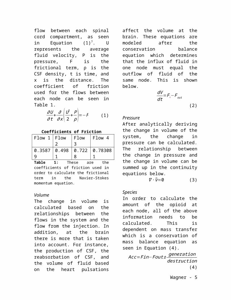
FlowThe flow of the system is pressure driven and can be calculated by the initial pressure conditions, velocity, and the resistance of flow at that point. The initial pressure of the brain is a sinusoidal function with the frequency of 1.5 Hz, which is approximately the average heart rate frequency, while all the other nodes’ initial pressures were set to zero6. Navier-Stokes momentum equation was used in order to calculate the flow between each spinal cord compartment, as seen in Equation (1)7. U represents the average fluid velocity, P is the pressure, F is the frictional term, ρ is the CSF density, t is time, and x is the distance. The coefficient of friction used for the flows between each node can be seen in Table 1.

∂U∂t

+ ∂∂ x ( U 2

2+ P

ρ )=−F (1)

Coefficients of FrictionFlow 1 Flow 2 Flow 3 Flow 40.35879 0.4981 0.7228 0.783081Table 1: These are the coefficients of friction used in order to calculate the frictional term in the Navier-Stokes momentum equation.

VolumeThe change in volume is calculated based on the relationships between the flows in the system and the flow from the injection. In addition, at the brain there is more that is taken into account. For instance, the production of CSF, the reabsorbation of CSF, and the volume of fluid based on the heart pulsations affect the volume at the brain. These equations are modeled after the conservation balance equation which determines that the influx of fluid in one node must equal the outflow of fluid of the same node. This is shown below.

dVdt

=F¿−Fout (2)

PressureAfter analytically deriving the change in volume of the system, the change in pressure can be calculated. The relationship between the change in pressure and the change in volume can be summed up in the continuity equations below.

∇ ∙ v⃗=0 (3)

SpeciesIn order to calculate the amount of the opioid at each node, all of the above information needs to be calculated. This is dependent on mass transfer which is a conservation of mass balance equation as seen in Equation (4).

Acc=Fin−Fout ± generationdestruction (4)

Since the flows are bidirectional, a method was determined to decide which

Wagner - 3

flow and concentration combination to use at a specific time. Therefore, for each possible flow into the node the maximum was taken between that flow and concentration relationship and zero. Since the flow can only occur in one direction, if one of the flow and concentration relationships where negative while the other positive using the above method the positive one would be used in the calculation. Furthermore, if both were positive values, then both flows and concentrations would be taken into account by adding them together. It should be noted that during this calculation any flow and concentration that flowed from the Sacral region to the brain instead of flowing from the brain to the Sacral region was taken as a negative value before finding the maximum between that and zero. This is because when determining the equations it was all taken as the flow from the brain towards the Sacral region as positive while the reverse way as negative.

The species balance also took into account the effects of transferring into different tissues. These parameters are taken into account in the efflux of fluid from the compartment.

In addition, the destruction term at the end will have a different reaction rate value, k, depending on which opioid is being tested and for what tissue it is moving in. The reaction rates that were used can be seen in Table 21.

Kinetic TermsKinetic Morphine Alfentanil Fentanyl Sufentanilkic 0.037 0.17 0.0339 0.020kci 0.0143 0.0236 0.0159 0.0095kplc 0.0082 0.0868 0.0080 0.0131kie 0.0542 0.1372 0.1078 0.0291kei 0.0021 0.0063 0.0285 0.0137kplepi 0.0199 0.0201 0.1088 0.0323

Table 2: Above shows the kinetic terms for each opioid that was tested and how the react based on which tissue they are transferring from. kic

and kie are the rate constants for movement from the intrathecal space into the spinal cord and epidural space respectfully. On the other hand, kci and kei have the opposite movement of their counterparts above. kplc is the rate constant for movement from the spinal cord into the plasma and kplepi is movement from the epidural space into the plasma1.

ModelsThree different models were tested. These models are all under the same conditions and measured the same results but varied in how the flow equations were derived from the Navier-Stokes momentum equation. Model 1 is the simplest version which only takes into account the change in pressure and the frictional term. This can be seen in Equation (5).

∂ f∂ t

=∂ P∂ x

−F (5)

The second and third models both take into account the CSF densities. In the second model the flow is derived based on the velocity and pressure before and after the flow being calculated, as well as, the frictional term. This is depicted in Equation (6) below.

∂ f i

∂ t=[(U i−1+

Pi−1

ρ )−(U i+1+Pi

ρ )]−F (6)

The third model is similar to the second except that it takes into account the velocity and pressure before and the velocity and pressure of the current flow that is being calculated. This is seen in Equation (7).

∂ f i

∂ t=[(U i−1+

Pi−1

ρ )−(U i+Pi

ρ )]−F (7)

Wagner - 4

ResultsFlowBefore the injection at the 5 minute mark there is a sinusoidal steady flow between the compartments. In addition, there is a noticeable phase shift between the flows both before and after the injection. Once the injection takes place there is a large, instantaneous spike in the flow from the Lumbar compartment to the Sacral one. After fifteen minutes, the flow returns to a periodical wave form. This can be seen in Figure 3.

VolumeSince the initial conditions for volume of the brain was determined to be 55 mL, Cervical 23 mL, Thoracic 33 mL, Lumbar 25 mL, and Sacral 19 mL. Similar to the flow, Figure 4 shows how before the injection at the 5 minute mark the volumes periodically oscillate in the amount of fluid that is held at that compartment. When the injection occurs there is a large spike in volume in the brain that peaks at twice as much volume as before. The other compartments see this increase as well but at different times. The Lumbar increases first while the phase shift has the brain’s volume increasing last. After fifteen minutes most of the volumes return to approximately the same as before the injection. The brain on the other hand is still decreasing in volume even at the fifty minute mark

Figure 3: Above is the pressure based flow of the system in mL/s. The flows oscillate with a magnitude based on the amplitude received from the heart beat and injection rate. This explains why after 5 minutes the flow from the Lumbar region of the spine to the Sacral increases. Over time the flow a dynamic steady state and no longer has variation in the flow5.

Figure 4: This represents the change in volume of each compartment that was modeled over time. The oscillating volumes are due to the sinusoidal pulse of the heart. At the five minute mark the injection begins and is reflected in the volume of reach node. After the increase in volume there is a steady decline until the oscillations return to the initial periodic volume.

PressureThe change in pressure of mmHg over time of the system can be seen in Figure 5. Similar to both the volume and flow, there is a phase shift in the pressure before and after the Bolus injection. Due to the large amount of volume in the brain there is a large amount of pressure

Wagner - 5

0 5 10 15 20 25 30 35 40 45 50-400

-300

-200

-100

0

100

200

300Flow

f1f2f3f4

0 5 10 15 20 25 30 35 40 45 500

20

40

60

80

100

120Volume

V1V2V3V4V5

within that compartment as well. Over time there starts to be a decrease in pressure in each compartment.

0 5 10 15 20 25 30 35 40 45 50-100

0

100

200

300

400

500

600

700Pressure

P1P2P3P4P5

Figure 5: This figure describes the change in pressure in mmHg over time through each. Until the opioid was introduced there was a constant periodic pressure. After the injection was administered, there is an increase in pressure over time in each compartment with a steady decline over time.

SpeciesThe amount of species within the system was traced in the CSF space, spinal cord, epidural space, and the vasculature for each opioid. All of this can be seen in Figures 6-9. Overall, Alfentanil was removed from the system the fastest, Morphine lasted the longest and Fentanyl and Sufentanil were intermediate when compared to the other opioids. Alfentanil reached a zero concentration in the CSF space faster than the other opioids and reached a zero concentration in the spinal cord as well, which the other opioids did not. Contrastly, the opioid that transferred from the epidural space the fastest was Fentanyl. Lastly, during this time span each opioid was still increasing when they transferred to the vasculature.

Wagner - 6

0 5 10 15 20 25 30 35 40 45 50-0.5

0

0.5

1

1.5

2

2.5Drug Concentration in CSF space for Morphine

C1C2C3C4C5

0 5 10 15 20 25 30 35 40 45 50-0.5

0

0.5

1

1.5Drug Concentration in CSF space for Alfentanil

C1C2C3C4C5

0 5 10 15 20 25 30 35 40 45 50-0.5

0

0.5

1

1.5

2

2.5Drug Concentration in CSF space for Fentanyl

C1C2C3C4C5

0 5 10 15 20 25 30 35 40 45 50-0.5

0

0.5

1

1.5

2Drug Concentration in CSF space for Sufentanil

C1C2C3C4C5

Figure 6: These plots are the change in concentration in moles over time in minutes at the CSF space. A Shows that Morphine lasts the longest within the tissue. B Shows that Alfentanil is removed the fastest from the tissue. While C Fentanyl and D Sufentanyl are intermediate concentrations.

Figure 7: These plots are the change in concentration in moles over time in minutes at the spinal cord. Shows that Morphine lasts the longest within the tissue. B Shows that Alfentanil is removed the fastest from the tissue. While C Fentanyl and D Sufentanyl are intermediate.

Each opioid concentration was also compared through space and time. This is done by finding the concentration at each compartment at the same time. This can be seen in Figure 10. It can be seen that at the earliest time is the largest concentration of each opioid and as time passes the concentration lowers. Also, there is more of each opioid seen at the Lumbar and Sacral

nodes than at the Brain, Cervical and Thoracic. In addition, Alfentanil contains the lowest amount of concentration at each time and at each compartment. Similarly, Morphine has the largest concentration while Fentanyl and Sufentanil are the opioids that are in between compared to the rest. This is consistent with the results from before.

Wagner - 7

A B

C D

0 5 10 15 20 25 30 35 40 45 500

0.1

0.2

0.3

0.4Drug Concentration in SC for Morphine

C1C2C3C4

0 5 10 15 20 25 30 35 40 45 50-0.05

0

0.05

0.1

0.15Drug Concentration in SC for Alfentanil

C1C2C3C4

0 5 10 15 20 25 30 35 40 45 50-0.05

0

0.05

0.1

0.15

0.2

0.25

0.3Drug Concentration in SC for Fentanyl

C1C2C3C4

0 5 10 15 20 25 30 35 40 45 50-0.05

0

0.05

0.1

0.15

0.2

0.25

0.3Drug Concentration in SC for Sufentanil

C1C2C3C4

A B

C D

Figure 8: These plots are the change in concentration in moles over time in minutes at the epidural space. There are only four concentrations shown here opposed to the five concentrations from Figure 6 because the brain compartment does not transfer fluid directly into the epidural space. A Shows that Morphine lasts the longest within the tissue. B Shows that Alfentanil is removed slower from the system and starts to level

off. C Fentanyl is removed the fastest form this tissue and D Sufentanyl is starting to level off and soon decline like with Alfentanil.

Figure 9: These plots are the change in concentration in moles over time in minutes at the vasculature tissue. There are only four cocentrations shown here opposed to the five concentrations from Figure 6 because the brain compartment does not transfer fluid directly into the vasculature. A Shows that Morphine lasts the longest within the tissue since it is still increasing at a higher level of concentration for each nod. B Shows that Alfentanil is removed the fastest from the system and starts to level off at a lower concentration than the other opioids. C Fentanyl is removed faster form this tissue than Sufentanil. D Sufentanyl is still increasing like Morphine but at a lesser concenttartion.

Wagner - 8

0 5 10 15 20 25 30 35 40 45 50-0.1

0

0.1

0.2

0.3

0.4

0.5

0.6Drug Concentration in EPI for Morphine

C1C2C3C4

0 5 10 15 20 25 30 35 40 45 50-0.1

0

0.1

0.2

0.3

0.4Drug Concentration in EPI for Alfentanil

C1C2C3C4

0 5 10 15 20 25 30 35 40 45 50-0.1

0

0.1

0.2

0.3

0.4

0.5

0.6Drug Concentration in EPI for Fentanyl

C1C2C3C4

0 5 10 15 20 25 30 35 40 45 50-0.05

0

0.05

0.1

0.15

0.2

0.25

0.3Drug Concentration in EPI for Sufentanil

C1C2C3C4

A B

C D

0 5 10 15 20 25 30 35 40 45 50-0.1

0

0.1

0.2

0.3

0.4

0.5

0.6Drug Concentration in VASC for Morphine

C1C2C3C4

0 5 10 15 20 25 30 35 40 45 50-0.2

0

0.2

0.4

0.6

0.8

1Drug Concentration in VASC for Alfentanil

C1C2C3C4

0 5 10 15 20 25 30 35 40 45 50-0.2

0

0.2

0.4

0.6

0.8

1

1.2Drug Concentration in VASC for Fentanyl

C1C2C3C4

0 5 10 15 20 25 30 35 40 45 50-0.1

0

0.1

0.2

0.3

0.4Drug Concentration in VASC for Sufentanil

C1C2C3C4

A B

C D

Figure 10: Each plot shows the concentration at a given compartment of the system. Each line corresponds to a different time in minutes. This mimics the results seen in previous figures but shows the results according to position within the system instead of the concentration as a function of time. A shows the concentration of Morphine. B shows the concentration of Fentanyl. C shows the concentration of Alfentanil and D shows the concentration of Sufentanil.ModelsEach of the three models were plotted together in order to compare the effects of different flow equations on the system. Figure 11 shows each model plotted together and compared between the volume, pressure, flow, and concentration with Morphine. It can be

seen that Model 1 and Model 2 are almost identical but vary slightly while Model 3 has the greatest amount of differences. Model 3 has the flow from the Bolus injection return to the original state earlier than the others and with les amplitude.

Wagner - 9

Brain Cervical Thoracic Lumbar Sacral0

0.5

1

1.5

2Concentration of Morphine at Each Compartment at a Given Time

Compartment

Con

cent

ratio

n

Brain Cervical Thoracic Lumbar Sacral0

0.5

1

1.5

2Concentration of Fentanyl at Each Compartment at a Given Time

Compartment

Con

cent

ratio

n

Brain Cervical Thoracic Lumbar Sacral0

0.2

0.4

0.6

0.8

1

1.2

1.4Concentration of Alfentanil at Each Compartment at a Given Time

Compartment

Con

cent

ratio

n

Brain Cervical Thoracic Lumbar Sacral0

0.5

1

1.5Concentration of Sufentanil at Each Compartment at a Given Time

Compartment

Con

cent

ratio

n

A B

C D

A B

C D

Figure 11: Each plot compares the three different models that was tested. The blue line is Model 1, the red line is Model 2, and the black line is Model 3. Model 3 shows the injection having the least effect on the system and Models 1 and 2 are almost identical in the effect they take on the system. A compares the difference in volume, B the difference in pressure, C the difference in flow, and D the difference in concentration that the different representations of flow have.Discussion The phase shift that is common between the flow, volume, and pressure occurs because of the pulsations from the heart beat. The flow is first seen in the brain and then proceeds to the lower compartments of the spinal cord. Since there is internal resistance to the fluid and the length affects the velocity of the fluid there is a delay in the flow seen throughout the system. Furthermore, since the flow of CSF affects the volume which in turn affects the pressure, the phase shift is also seen in both of these parameters.

The flow of CSF in the system increases when the injection occurs and then begins to return to its original state. The reason it does not stay at the amplitude and frequency that is a direct cause of the injection is because of the type of injection that is used. Since a Bolus injection was tested in this model there is only an inlet of opioid for thirty seconds. Afterwards there is no more influx of fluid into the system allowing it

to return to the original steady state over time.

There are two possible ways that the CSF could be dispersed within the brain. Either it can swell the fluid filled sac that surrounds the brain or it can be reabsorbed into the surrounding tissue. According to the model created the extra CSF fluid in the brain swells the surrounding fluid sac. This is depicted in Figure 4. Since there is a large increase in volume due to the Bolus injection that takes a noticeable longer time to start to return to normal than the other spinal cord compartments, it can be deduced that this is not because of reabsorption. As seen in Figure 1, the brain does not have an absorption term to the epidural space and vasculature like the spinal cord compartments do. The result is that the extra fluid in the brain is stagnate until it can be redistributed elsewhere.

The resulting concentrations are similar to what was expected based on the work of Ummenhofer et al. The only discrepancy is found with the opioid

Wagner - 10

0 5 10 15 20 25 30 35 40 45 500

20

40

60

80

100

120Model Comparision: Volume

0 5 10 15 20 25 30 35 40 45 50-2000

-1000

0

1000

2000

3000

4000

5000Model Comparision: Pressure

0 5 10 15 20 25 30 35 40 45 50-400

-300

-200

-100

0

100

200

300Model Comparision: Flow

0 5 10 15 20 25 30 35 40 45 50-0.5

0

0.5

1

1.5

2

2.5

3Model Comparision: Morphine Concentration in the Spinal Cord

with the least amount of concentration. Ummenhofer et al stated that Fentanyl would contain the smallest concentration over time while it was modeled here as close to the largest, yet still an intermediate drug1. The opioid with the lowest concentration was modeled as Alfentanil at the end of the model. It is reasonable that Alfentanil has the least concentration based on its kinetic terms. Overall Alfentanil’s kinetics are higher than the other opioids observed. This had a great impact on the transfer between the different tissues. Some key differences between the two results is that Ummenhofer did not take into account the heart rate while this model did not take into account gravity or shear stress, both of which affect the Navier-Stokes momentum equation7. This could be the reason why the two results were slightly different.

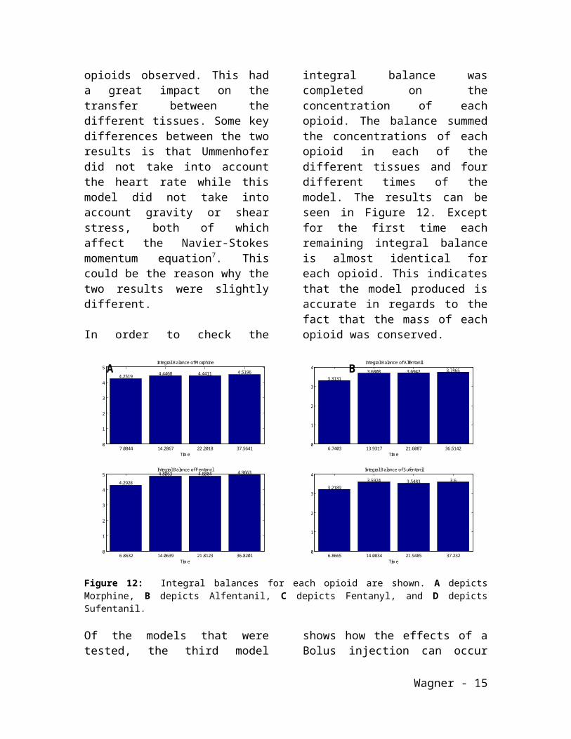
In order to check the accuracy of the model an integral balance was completed on the concentration of each opioid. The balance summed the concentrations of each opioid in each of the different tissues and four different times of the model. The results can be seen in Figure 12. Except for the first time each remaining integral balance is almost identical for each opioid. This indicates that the model produced is accurate in regards to the fact that the mass of each opioid was conserved.

Wagner - 11

Figure 12: Integral balances for each opioid are shown. A depicts Morphine, B depicts Alfentanil, C depicts Fentanyl, and D depicts Sufentanil.

Of the models that were tested, the third model shows how the effects of a Bolus injection can occur instantaneously and leave the system in a short amount of time. In order to determine if this is the most accurate model that was constructed either experimental data would need to be known in order to make a comparison or the model should be tested using a continuous injection to see if there are any major discrepancies there.

ConclusionThis model can be used in order to assist surgeons in deciding which opioid to use as an Anesthetic during any given procedure. All they would have to do is

decide on a timeframe for the procedure, what type of injection will be used, and approximate the frequency of the heartbeat. With all of these factors taken into account, they will be able to analyze the concentration graphs and make an educated decision on which opioid to use.

In order to further the accuracy of this model, the next step would be to analyze each vertebra instead of the four regions of vertebra in the spinal cord. This would allow for a more precise location of the opioid concentration in the system as well as allowing for increased accuracy in knowing the precise injection site location.

Wagner - 12

7.0844 14.2867 22.2018 37.56410

1

2

3

4

5Integral Balance of Morphine

Time

4.2519 4.4468 4.4411 4.5196

6.7403 13.9317 21.6087 36.51420

1

2

3

4Integral Balance of Alfentanil

Time

3.31313.6808 3.6942 3.7465

6.8632 14.0639 21.8123 36.82010

1

2

3

4

5Integral Balance of Fentanyl

Time

4.2928

4.8863 4.8804 4.9663

6.8665 14.0834 21.9485 37.2320

1

2

3

4Integral Balance of Sufentanil

Time

3.21893.5924 3.5483 3.6

A B

C D

Intellectual PropertyBiological and physiological data and some modeling procedures provided to you from Dr. Linninger’s lab are subject to IRB review procedures and Intellectual property procedures.

Therefore, the use of these data and procedures are limited to the coursework only. Publications need to be approved and require joint authorship with staff of Dr. Linninger’s lab.

Reference[1] Ummenhofer, Wolfgang C., et al. "Comparative spinal distribution and clearance

kinetics of intrathecally administered morphine, fentanyl, alfentanil, and sufentanil." Anesthesiology 92.3 (2000): 739-753.

[2] Hsu, Ying, et al. “The frequency and magnitude of cerebrospinal fluid pulsations influence intrathecal drug distribution: key factors for interpatient variability.” Anesthesia & Analgesia 115.2 (2012): 386-394

[3] Shafer, Steven L., and John R. Varvel. "Pharmacokinetics, pharmacodynamics, and rational opioid selection." Anesthesiology 74.1 (1991): 53-63.

[4] Jeffrey J. Iliff, PhD and Richard D. Penn, MD. “Fluid flow in the brain and the glymphatic system”

[5] Zhou Xuedong, et al. “Response on Harmonic Excitation Analysis.” (2005)[6] Berkow, Robert. The Merck Manual of Medical Information. New Jersey: Merck,

1997.[7] Zagzoule, Mokhtar and Jean-Pierre Marc-Verones. “A Global mathematical model of

the cerebral circulation in man.” J. Biomechanics. 19.12 (1986) 1015-1022

Wagner - 13

Appendix1: System Diagram

C = [7.5, 26; 7.5, 18; 7.5, 10; 7.5, 2 7.5, -6]; Lx = [7.5, 7.5; 7.5, 7.5; 7.5, 7.5; 7.5, 7.5 7.5, 7.5]; Ly = [32, 28; 24, 20; 16, 12; 8, 4 0, -4]; %labeling for i = 1:4 c = C(i,1)-1; cP = C(i,1)-5; text(c, C(i,2), ['V', num2str(i+1)]) cLx = C(i,1)+3; cLy = C(i,2)+4; text(cLx, C(i,2)+9, ['P', num2str(i)]) text(cLx, cLy, ['F', num2str(i)]) if i == 4 cLx = C(i+1,1)+3; cLy = C(i+1,2)+8; text(cLx, cLy+1, ['P', num2str(i+1)]) endend for i = 1:4 line(Lx(i,:), Ly(i,:), 'Color', 'k') %flow line downward end %labelingtext(6, 35, 'Brain')text(0, C(1,2), 'Cervical')text(0, C(2,2), 'Thoracic')text(0, C(3,2), 'Lumbar')text(0, C(4,2), 'Sacral')text(6, 33, 'V1')axis([0 15 0 37])title('Spinal Cord Model')

Rx = [5; 10; 10; 5; 5];Ry = [32; 32; 37; 37; 32];line(Rx, Ry, 'Color', 'k') %brain rectangle RLx = [9.5; 15];RLy = [26; 26; 18; 18; 10; 10; 2; 2];for i = 2:2:8line(RLx, RLy(i-1:i), 'Color', 'k') %line to epidural spaceend Bx = [15; 20; 20; 15; 15];By = [0; 0; 28; 28; 0];line(Bx, By, 'Color', 'k') %epidural space boxh = text(17.5,12, 'Epidural Space');set(h, 'rotation', 90) line([20; 25], [18; 18], 'Color', 'k') %line to vasculature Bx = [25; 30; 30; 25; 25];By = [0; 0; 28; 28; 0];line(Bx, By, 'Color', 'k') %vasculature boxh = text(27.5,12,'Vasculature');set(h, 'rotation', 90) C = [7.5, 26; 7.5, 18; 7.5, 10; 7.5, 2 7.5, -6];r = [2; 2; 2; 2]; viscircles(C(1:4, :), r, 'Edgecolor', 'k', 'LineWidth', 1) %compartmentsaxis equal

Wagner - 14

Appendix 2: Deformation

%% normal/ idealfor i = 1:2:3 subplot(1,3,i) C = [7.5, 26; 7.5, 18; 7.5, 10; 7.5, 2 7.5, -6]; Lx = [7.5, 7.5; 7.5, 7.5; 7.5, 7.5; 7.5, 7.5 7.5, 7.5]; Ly = [32, 28; 24, 20; 16, 12; 8, 4 0, -4]; %labelingfor i = 1:4 c = C(i,1)-1; cP = C(i,1)-5; text(c, C(i,2), ['V', num2str(i+1)]) cLx = C(i,1)+3; cLy = C(i,2)+4; text(cLx, C(i,2)+8, ['P', num2str(i)]) text(cLx, cLy, ['F', num2str(i)]) if i == 4 cLx = C(i+1,1)+3; cLy = C(i+1,2)+8; text(cLx, cLy, ['P', num2str(i+1)]) endend %flow lines for i = 1:4 line(Lx(i,:), Ly(i,:), 'Color', 'k') end %labelingtext(6, 35, 'Brain')text(0, C(1,2), 'Cervical')text(0, C(2,2), 'Thoracic')

text(0, C(3,2), 'Lumbar')text(0, C(4,2), 'Sacral')text(6, 33, 'V1')axis([0 15 0 37])title('Spinal Cord Model') %brain rectangleRx = [5; 10; 10; 5; 5];Ry = [32; 32; 37; 37; 32];line(Rx, Ry, 'Color', 'k') C = [7.5, 26; 7.5, 18; 7.5, 10; 7.5, 2 7.5, -6];r = [2; 2; 2; 2]; %compartments viscircles(C(1:4, :), r, 'Edgecolor', 'k', 'LineWidth', 1)axis equalend %% deformationsubplot(1,3,2) C = [7.5, 26; 7.5, 18; 7.5, 10; 7.5, 2 7.5, -6]; Lx = [7.5, 7.5; 7.5, 7.5; 7.5, 7.5; 7.5, 7.5 7.5, 7.5]; Ly = [32, 29.5; 22.5, 21; 15, 12.5; 7.5, 4 0, -4]; %labelingfor i = 1:4 c = C(i,1)-1; cP = C(i,1)-5; text(c+0.5, C(i,2), ['V', num2str(i+1)]) cLx = C(i,1)+3; cLy = C(i,2)+4;

Wagner - 15

text(cLx+1, C(i,2)+8, ['P', num2str(i)]) text(cLx+1, cLy, ['F', num2str(i)]) if i == 4 cLx = C(i+1,1)+4; cLy = C(i+1,2)+8; text(cLx, cLy, ['P', num2str(i+1)]) endend for i = 1:4 line(Lx(i,:), Ly(i,:), 'Color', 'k') %flow lines end %labelingtext(6.5, 35, 'Brain')text(0, C(1,2), 'Cervical')text(0, C(2,2), 'Thoracic')text(0, C(3,2), 'Lumbar')text(0, C(4,2), 'Sacral')

text(7, 33, 'V1')axis([0 15 0 37])title('Spinal Cord Model with Deformation') Rx = [5; 10; 10; 5; 5];Ry = [32; 32; 37; 37; 32]; line(Rx, Ry, 'Color', 'k') %brain rectangle C = [7.5, 26; 7.5, 18; 7.5, 10; 7.5, 2 7.5, -6];r = [3.5; 3; 2.5; 2]; %compartmentsviscircles(C(1:4, :), r, 'Edgecolor', 'k', 'LineWidth', 1)

Wagner - 16

Appendix 3: Brain ODEfunction FP_Mainclear all; close all; clc;y0 = zeros(30,1);y0(1:5)=[55;23;33;25;19];global jfor j = 1:4[T,Y] = ode45(@brainwaiver ,[0 50],y0);save('model1','Y','T'); V = Y(:,1:5);P = .0075*Y(:,6:9);P0 =V(:,1)/.188;F = Y(:,10:13); if j ==1TM=T; CM = Y(:,14:18);CMsc = Y(:,19:22); CMepi = Y(:,23:26);CMvas = Y(:,27:30);end if j ==2TA=T; CA = Y(:,14:18);CAsc = Y(:,19:22); CAepi = Y(:,23:26);CAvas = Y(:,27:30);end if j ==3TF=T; CF = Y(:,14:18);CFsc = Y(:,19:22); CFepi = Y(:,23:26);CFvas = Y(:,27:30);end if j ==4TS=T; CS = Y(:,14:18);CSsc = Y(:,19:22); CSepi = Y(:,23:26);CSvas = Y(:,27:30);end end PLOTME(TM,TA,TF,TS, V, P, P0, F, CM, CMsc, CMepi, CMvas, CA, CAsc, CAepi, CAvas, CF, CFsc, CFepi, CFvas, CS, CSsc, CSepi, CSvas)

Wagner - 17

function dP = brainwaiver(t,Y)kappa = [.188;.0210;.0174;.0126;.0139]; K = 1./kappa;E=1; alfa = [.35879;.49138;.7228;.783081];Fprod = 0;reab=6.4e-4;timei=5;Pven=0;A=2;w=1*pi;rho = 1.0068; % Finj = 1;if (t >=timei && t <=(timei+0.05)) Finj = 1000; %.05sec*1000=50mL Co=1;else Finj = 0; Co=0;end V = Y(1:5); CA= .75;P = Y(6:9);U = Y(10:13);F = CA*U; % VolumedP(1,1) = Fprod-F(1)-max(0,((P(1)-Pven)*reab))+A*cos(w*t)*w;dP(2,1) = (F(1) - F(2));dP(3,1) = (F(2) - F(3));dP(4,1) = (F(3) - F(4))+ Finj;dP(5,1) = (F(4));P0 = V(1)*K(1); % PressuredP(6,1) = K(2)*dP(2,1); % P2dP(7,1) = K(3)*dP(3,1); % P3dP(8,1) = K(4)*dP(4,1); % P4dP(9,1) = K(5)*dP(5,1); % P5 %Flow Model 1:dP(10,1) = (P0-P(1))-(U(1)*alfa(1));dP(11,1) = (P(1)-P(2))-(U(2)*alfa(2));dP(12,1) = (P(2)-P(3))-(U(3)*alfa(3));dP(13,1) = (P(3)-P(4))-(U(4)*alfa(4)); % %Flow Model 2:% dP(10,1) = (P0/rho)-((U(2))+P(1)/rho)-(U(1)*alfa(1));% dP(11,1) = ((U(1))+P(1)/rho)-((U(3))+P(2)/rho)-(U(2)*alfa(2));% dP(12,1) = ((U(2))+P(2)/rho)-((U(4))+P(3)/rho)-(U(3)*alfa(3));% dP(13,1) = ((U(3))+P(3)/rho)-(P(4)/rho)-(U(4)*alfa(4)); % % Flow Model 3:% dP(10,1) = (P0/rho)-((U(1))+P(1)/rho)-(U(1)*alfa(1));

Wagner - 18

% dP(11,1) = ((U(1))+P(1)/rho)-((U(2))+P(2)/rho)-(U(2)*alfa(2));% dP(12,1) = ((U(2))+P(2)/rho)-((U(3))+P(3)/rho)-(U(3)*alfa(3));% dP(13,1) = ((U(3))+P(3)/rho)-((U(4))+P(4)/rho)-(U(4)*alfa(4)); C = Y(14:18);concSCstart=19;%where spinal cord tissue startsconcSCend=22; %where spinal cord tissue endsCsc = Y(concSCstart:concSCend); concEPIstart = 23; %where epidural space startsconcEPIend = 26; %where epidural space endCepi = Y(concEPIstart:concEPIend); concVASCstart = 27; %where vasculature startsconcVASCend = 30; %where vasculature endsCvas = Y(concVASCstart:concVASCend); KIC = [0.037 0.170 0.0339 .020]; %%CSF space to SC [MAFS]KCI = [0.0143 0.0236 0.0159 0.0095]; %%SC to CSF spaceKIE = [0.0542 0.1372 0.1078 0.0291]; %%CSF space to Epidural spaceKEI = [0.0021 0.0063 0.0285 0.0137]; %%Epidural space to SCFKPLC = [0.0082 0.868 0.0080 0.0131]; %%SC to Vasclature KPLEPI = [0.0199 0.0201 0.1088 0.0323]; %Umenhofer % Concentrationglobal jdP(14,1) = (-max(0,C(1)*F(1))+max(0,-F(1)*C(2)))/V(1);%concetration leaving the braindP(15,1) = (-max(0,C(2)*F(2))+max(0,-F(2)*C(3))+max(0,C(1)*F(1))...-max(0,-F(1)*C(2)))/V(2)-KIC(j)*C(2)+KCI(j)*Csc(1)-KIE(j)*C(2)+KEI(j)*Cepi(1);dP(16,1) = (-max(0,C(3)*F(3))+max(0,-F(3)*C(4))+max(0,C(2)*F(2))...-max(0,-F(2)*C(3)))/V(3)-KIC(j)*C(3)+KCI(j)*Csc(2)-KIE(j)*C(3)+KEI(j)*Cepi(3);dP(17,1) = (-max(0,C(4)*F(4))+max(0,-F(4)*C(5))+max(0,C(3)*F(3))...-max(0,-F(3)*C(4))+Finj*Co)/V(4)-KIC(j)*C(4)+KCI(j)*Csc(3)-KIE(j)*C(4)+KEI(j)*Cepi(3);dP(18,1) = (max(0,C(4)*F(4))-max(0,-F(4)*C(5)))/V(5)-KIC(j)*C(5)+KCI(j)*Csc(4)...-KIE(j)*C(5)+KEI(j)*Cepi(4); for i = concSCstart:concSCend dP(i,1) = KIC(j)*C(i-17)-KCI(j)*Csc(i-18)-KPLC(j)*Csc(i-18);endfor i = concEPIstart:concEPIend dP(i,1) = KIE(j)*C(i-concSCend+1)-KEI(j)*Cepi(i-concSCend)-KPLEPI(j)*Cepi(i-concSCend);end for i = concVASCstart:concVASCend dP(i,1) = KPLC(j)*Csc(i-concEPIend)+KPLEPI(j)*Cepi(i-concEPIend); end

Wagner - 19

function PLOTME(TM, TA,TF,TS, V, P, P0, F, CM, CMsc, CMepi, CMvas, CA, CAsc, CAepi, CAvas, CF, CFsc, CFepi, CFvas, CS, CSsc, CSepi, CSvas) %integral balancesfor k = 500:500:2000S_M(k/500) = sum(CM(k,:))+sum(CMsc(k,:))+sum(CMepi(k,:))+sum(CMvas(k,:));S_A(k/500) = sum(CA(k,:))+sum(CAsc(k,:))+sum(CAepi(k,:))+sum(CAvas(k,:));S_F(k/500) = sum(CF(k,:))+sum(CFsc(k,:))+sum(CFepi(k,:))+sum(CFvas(k,:));S_S(k/500) = sum(CS(k,:))+sum(CSsc(k,:))+sum(CSepi(k,:))+sum(CSvas(k,:));end figuresubplot(2,2,1)bar(S_M)title('Integral Balance of Morphine')set(gca, 'XTickLabel', {num2str(TM(500)), num2str(TM(1000)), num2str(TM(1500)), num2str(TM(2000))})xlabel('Time') for i = 1:4text(i,S_M(i)+.35, num2str(S_M(i)), 'HorizontalAlignment','center','VerticalAlignment','top')end subplot(2,2,2)bar(S_A)title('Integral Balance of Alfentanil')set(gca, 'XTickLabel', {num2str(TA(500)), num2str(TA(1000)), num2str(TA(1500)), num2str(TA(2000))})xlabel('Time') for i = 1:4text(i,S_A(i)+.25, num2str(S_A(i)), 'HorizontalAlignment','center','VerticalAlignment','top')end subplot(2,2,3)bar(S_F)title('Integral Balance of Fentanyl')set(gca, 'XTickLabel', {num2str(TF(500)), num2str(TF(1000)), num2str(TF(1500)), num2str(TF(2000))})xlabel('Time') for i = 1:4text(i,S_F(i)+.35, num2str(S_F(i)), 'HorizontalAlignment','center','VerticalAlignment','top')end subplot(2,2,4)bar(S_S)title('Integral Balance of Sufentanil')

Wagner - 20

set(gca, 'XTickLabel', {num2str(TS(500)), num2str(TS(1000)), num2str(TS(1500)), num2str(TS(2000))})xlabel('Time') for i = 1:4text(i,S_S(i)+.25, num2str(S_S(i)), 'HorizontalAlignment','center','VerticalAlignment','top')end %Concentration at nodesnode = 1:5;t = [500; 1000; 1500; 2000];%, floor(length(TS)/4), floor(length(TS)/2), floor(length(TS))];figuresubplot(2,2,1)plot(node, CM(t(1),:), node, CM(t(2),:), node, CM(t(3),:), node, CM(t(4),:))title('Concentration of Morphine at Each Compartment at a Given Time')set(gca, 'XTickLabel', {'Brain',' ', 'Cervical', ' ', 'Thoracic', ' ', 'Lumbar', ' ', 'Sacral'})xlabel('Compartment')ylabel('Concentration') subplot(2,2,2)plot(node, CF(t(1),:), node, CF(t(2),:), node, CF(t(3),:), node, CF(t(4),:))title('Concentration of Fentanyl at Each Compartment at a Given Time')set(gca, 'XTickLabel', {'Brain',' ', 'Cervical', ' ', 'Thoracic', ' ', 'Lumbar', ' ', 'Sacral'})xlabel('Compartment')ylabel('Concentration') subplot(2,2,3)plot(node, CA(t(1),:), node, CA(t(2),:), node, CA(t(3),:), node, CA(t(4),:))title('Concentration of Alfentanil at Each Compartment at a Given Time')set(gca, 'XTickLabel', {'Brain',' ', 'Cervical', ' ', 'Thoracic', ' ', 'Lumbar', ' ', 'Sacral'})xlabel('Compartment')ylabel('Concentration') subplot(2,2,4)plot(node, CS(t(1),:), node, CS(t(2),:), node, CS(t(3),:), node, CS(t(4),:))title('Concentration of Sufentanil at Each Compartment at a Given Time')set(gca, 'XTickLabel', {'Brain',' ', 'Cervical', ' ', 'Thoracic', ' ', 'Lumbar', ' ', 'Sacral'})xlabel('Compartment')ylabel('Concentration') %concentrationfigure; subplot(2,2,1)plot(TM,CM); title('Drug Concentration in CSF space for Morphine'); legend('C1' ,'C2', 'C3', 'C4', 'C5');subplot(2,2,2)

Wagner - 21

plot(TA,CA); title('Drug Concentration in CSF space for Alfentanil'); legend('C1' ,'C2', 'C3', 'C4', 'C5');subplot(2,2,3)plot(TF,CF); title('Drug Concentration in CSF space for Fentanyl'); legend('C1' ,'C2', 'C3', 'C4', 'C5');subplot(2,2,4)plot(TS,CS); title('Drug Concentration in CSF space for Sufentanil'); legend('C1' ,'C2', 'C3', 'C4', 'C5'); figure; subplot(2,2,1)plot(TM,CMsc); title('Drug Concentration in SC for Morphine'); legend('C1' ,'C2', 'C3', 'C4');subplot(2,2,2)plot(TA,CAsc); title('Drug Concentration in SC for Alfentanil'); legend('C1' ,'C2', 'C3', 'C4');subplot(2,2,3)plot(TF,CFsc); title('Drug Concentration in SC for Fentanyl'); legend('C1' ,'C2', 'C3', 'C4');subplot(2,2,4)plot(TS,CSsc); title('Drug Concentration in SC for Sufentanil'); legend('C1' ,'C2', 'C3', 'C4'); figure; subplot(2,2,1)plot(TM,CMepi); title('Drug Concentration in EPI for Morphine'); legend('C1' ,'C2', 'C3', 'C4');subplot(2,2,2)plot(TA,CAepi); title('Drug Concentration in EPI for Alfentanil'); legend('C1' ,'C2', 'C3', 'C4');subplot(2,2,3)plot(TF,CFepi); title('Drug Concentration in EPI for Fentanyl'); legend('C1' ,'C2', 'C3', 'C4');subplot(2,2,4)plot(TS,CSepi); title('Drug Concentration in EPI for Sufentanil'); legend('C1' ,'C2', 'C3', 'C4'); figure;subplot(2,2,1)plot(TM,CMvas); title('Drug Concentration in VASC for Morphine'); legend('C1' ,'C2', 'C3', 'C4');subplot(2,2,2)plot(TA,CAvas); title('Drug Concentration in VASC for Alfentanil'); legend('C1' ,'C2', 'C3', 'C4');subplot(2,2,3)plot(TF,CFvas); title('Drug Concentration in VASC for Fentanyl'); legend('C1' ,'C2', 'C3', 'C4');subplot(2,2,4)plot(TS,CSvas); title('Drug Concentration in VASC for Sufentanil'); legend('C1' ,'C2', 'C3', 'C4'); figure; plot(TS,V) ;title('Volume'); legend('V1', 'V2', 'V3', 'V4', 'V5');figure; plot(TS,[P0 P]) ;title('Pressure'); legend('P1', 'P2', 'P3', 'P4', 'P5');figure; plot(TS,F) ;title('flow'); legend('f1', 'f2', 'f3', 'f4');

Wagner - 22