Embed Size (px)
DESCRIPTION
butter filter
Citation preview

Linköping studies in science and technology. Thesis.No. 1527
Averaging level control in thepresence of frequent inlet flow upsets
Peter Rosander
REGLERTEKNIK
AUTOMATIC CONTROL
LINKÖPING
Division of Automatic ControlDepartment of Electrical Engineering
Linköping University, SE-581 83 Linköping, Swedenhttp://www.control.isy.liu.se
Linköping 2012

This is a Swedish Licentiate’s Thesis.
Swedish postgraduate education leads to a Doctor’s degree and/or a Licentiate’s degree.A Doctor’s Degree comprises 240 ECTS credits (4 years of full-time studies).
A Licentiate’s degree comprises 120 ECTS credits,of which at least 60 ECTS credits constitute a Licentiate’s thesis.
Linköping studies in science and technology. Thesis.No. 1527
Averaging level control in the presence of frequent inlet flow upsets
Peter Rosander
Department of Electrical EngineeringLinköping UniversitySE-581 83 Linköping
Sweden
ISBN 978-91-7519-919-1 ISSN 0280-7971 LiU-TEK-LIC-2012:12
Copyright © 2012 Peter Rosander
Printed by LiU-Tryck, Linköping, Sweden 2012

Till Maria

Abstract
Buffer tanks are widely used within the process industry to prevent flow varia-tions from being directly propagated throughout a plant. The capacity of thetank is used to smoothly transfer inlet flow upsets to the outlet. Ideally, the tankthus works as a low pass filter where the available tank capacity limits the achiev-able flow smoothing.
For infrequently occurring upsets, where the system has time to reach steadystate between flow changes, the averaging level control problem has been exten-sively studied. After an inlet flow change, flow filtering has traditionally beenobtained by letting the tank level deviate from its nominal value while slowlyadapting the outlet to cancel out the flow imbalance and eventually bringingback the level to its set-point. The system is then again in steady state and readyto surge the next upset. By ensuring that the single largest upset can be handledwithout violating the level constraints, satisfactory flow smoothing is obtained.
In this thesis, the smoothing of frequently changing inlet flows is addressed. Inthis case, standard level controllers struggle to obtain acceptable flow smoothingsince the system rarely is in steady state and flow upsets can thus not be treatedas separate events. To obtain a control law that achieves optimal filtering whiledirectly accounting for future upsets, the averaging level control problem wasapproached using robust model predictive control (MPC).
The robust MPC differs in the way it obtains flow smoothing by not returning thetank level to a fixed set-point. Instead, it lets the steady state tank level dependon the current value of the inlet flow. This insight was then used to propose a lin-ear control structure, designed to filter frequent upsets optimally. Analyses andsimulation results indicate that the proposed linear and robust MPC controllerobtain flow smoothing comparable to the standard optimal averaging level con-trollers for infrequent upsets while handling frequent upsets considerably better.
v


Populärvetenskaplig sammanfattning
Inom processindustrin används buffertankar för flera olika syften, såsom att lag-ra slutprodukter för att säkerställa snabb leverans av kundordrar eller som mel-lanlager, för att möjliggöra produktion trots att delar av en fabrik har ett drift-eller underhållsstopp. I den här avhandlingen behandlas fallet där buffertankaranvänds för att jämna ut flödesvariationer. Snabba flödesvariationer är inte önsk-värda då de kan störa produktionen. Exempelvis, kan destilleringen i en destilla-tionskolonn påverkas så att alla biprodukter inte destilleras bort och slutproduk-ten därmed inte går att sälja. Genom att använda buffertankar för flödesutjäm-ning hindras flödesvariationer från att fortplantas och påverka alla processer i enanläggning.
Buffertanken ska alltså fungera som ett filter mellan inflödet och utflödet, därvariationer på inflödet långsamt överförs till utflödet genom att tanknivån varie-ras. Efter en ändring av inflödet så åstadkoms flödesutjämning typiskt genomatt tanknivån först tillåts avvika från sitt nominella värde medan utflödet lång-samt anpassas till den nya produktstakten. Tanknivån förs sedan tillbaka till sittbörvärde och systemet är återigen redo att filtrera en flödesändring. Ju långsam-mare som utflödet ändras, desto bättre kommer filtrering att bli men desto merkommer också tanknivån att variera. Dock är tankkapaciteten begränsad vilketmåste beaktas vid trimningen av regulatorn. För flöden där förändringar sker säl-lan blir trimningen ganska enkel. Systemet kommer alltid att vara i stationaritet,alltså att tanken är på sitt börvärde och att in- och utflödet är lika, när en flö-desförändring sker. Det gör att varje variation av inflödet kan ses som en enskildhändelse. Genom att se till att regulatorn kan hantera den enskilt största flödes-förändringen, så kommer alla flödesvariationer att filtreras och tanken kommerinte att svämma över.
I den här avhandlingen behandlas flödesutjämning när flödesändringar är fre-kventa. Flödesändringarna kan inte längre ses som separata händelser då syste-met sällan kommer att vara i stationaritet när inflödet ändras. Regulatorn kandärmed inte bara fokusera på att jämna ut den nuvarande flödesändringen utanmåste också alltid vara beredd på att nya ändringar kan uppstå.
Genom att använda en regulator som är baserad på robust optimering så har enstyrlag erhållits som uppnår optimal flödesutjämning för frekventa flödesvaria-tioner. Regulatorn skiljer sig mot de flesta standardregulatorer då den, efter enförändring av inflödet, inte återför tanknivån till ett fixt värde. Istället så berorden stationära tanknivån på vilket värde som inflödet för tillfället har. Linjäraregulatorer som också anpassar den stationära tanknivån har också föreslagits.Dessa regulatorer har sedan analyserats och visats erhålla jämförbar flödesutjäm-ning som tidigare kända regulatorer, när flödesändringar sker sällan. Simulering-ar med verkliga indata indikerar att de föreslagna regulatorerna däremot fun-gerar avsevärt bättre jämfört med standardregulatorer då flödesändringar skerofta.
vii

Acknowledgments
First of all, I want to thank my supervisors Prof. Alf Isaksson and Dr. Johan Löf-berg for guiding and supporting me in my PhD studies. Dr. Krister Forsmanat Perstorp AB has also been very influential in my research by providing ideasand interesting research topics. Without the three of you, this Licentiate’s thesiswould still lie several years into the future.
I am forever grateful to the former head of the group, Prof. Lennart Ljung, for let-ting me join the Automatic Control group, which nowadays is under the excellentleadership of Prof. Svante Gunnarsson. All administrative issues have skillfullybeen sorted out by the very helpful division coordinators Ninna Stensgård andher predecessor Åsa Karmelind.
The financial support from SSF, the Swedish Foundation for Strategic Research, aspart of Process Industry Centre Linköping, PIC-LI, is gratefully acknowledged.
The quality of this thesis has been greatly improved by the thorough proof-readingof my supervisors as well as my fellow PhD students Lic. André Carvalho Bitten-court, Lic. Patrik Axelsson and M.Sc. Daniel Simon. Your comments and sugges-tions were truly appreciated, although I must admit that I did not have the timeto implement all of them. Thanks also to Dr. Henrik Tidefeldt and Dr. GustafHendeby for their work in developing the LATEX template which was used to pro-duce this thesis.
A high-altitude thanks to the climbing section within the control group: Lic. An-dré Carvalho Bittencourt, Lic. Fredrik Lindsten and Dr. Tomas Schön, for all thefun I’ve had at the crag. To you, I say only one thing: Don’t fall!
Thanks to my roommate (well, at least during afternoons, evenings and week-ends) M.Sc. Tohid Ardeshiri for great company and interesting discussions.
Last but not least, I want to thank my family for supporting and encouragingme in every adventure I undertake, so also this. A very special thanks, fromthe bottom of my heart, to my wonderful Maria. Your love and support is never-ending and now when this thesis is finished, I’ll be all yours ;)
Linköping, April 2012Peter Rosander
ix

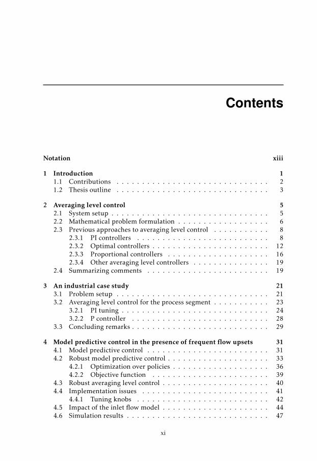
Contents
Notation xiii
1 Introduction 11.1 Contributions . . . . . . . . . . . . . . . . . . . . . . . . . . . . . . 21.2 Thesis outline . . . . . . . . . . . . . . . . . . . . . . . . . . . . . . 3
2 Averaging level control 52.1 System setup . . . . . . . . . . . . . . . . . . . . . . . . . . . . . . . 52.2 Mathematical problem formulation . . . . . . . . . . . . . . . . . . 62.3 Previous approaches to averaging level control . . . . . . . . . . . 8
2.3.1 PI controllers . . . . . . . . . . . . . . . . . . . . . . . . . . 82.3.2 Optimal controllers . . . . . . . . . . . . . . . . . . . . . . . 122.3.3 Proportional controllers . . . . . . . . . . . . . . . . . . . . 162.3.4 Other averaging level controllers . . . . . . . . . . . . . . . 19
2.4 Summarizing comments . . . . . . . . . . . . . . . . . . . . . . . . 19
3 An industrial case study 213.1 Problem setup . . . . . . . . . . . . . . . . . . . . . . . . . . . . . . 213.2 Averaging level control for the process segment . . . . . . . . . . . 23
3.2.1 PI tuning . . . . . . . . . . . . . . . . . . . . . . . . . . . . . 243.2.2 P controller . . . . . . . . . . . . . . . . . . . . . . . . . . . 28
3.3 Concluding remarks . . . . . . . . . . . . . . . . . . . . . . . . . . . 29
4 Model predictive control in the presence of frequent flow upsets 314.1 Model predictive control . . . . . . . . . . . . . . . . . . . . . . . . 314.2 Robust model predictive control . . . . . . . . . . . . . . . . . . . . 33
4.2.1 Optimization over policies . . . . . . . . . . . . . . . . . . . 364.2.2 Objective function . . . . . . . . . . . . . . . . . . . . . . . 39
4.3 Robust averaging level control . . . . . . . . . . . . . . . . . . . . . 404.4 Implementation issues . . . . . . . . . . . . . . . . . . . . . . . . . 41
4.4.1 Tuning knobs . . . . . . . . . . . . . . . . . . . . . . . . . . 424.5 Impact of the inlet flow model . . . . . . . . . . . . . . . . . . . . . 444.6 Simulation results . . . . . . . . . . . . . . . . . . . . . . . . . . . . 47
xi
xii CONTENTS
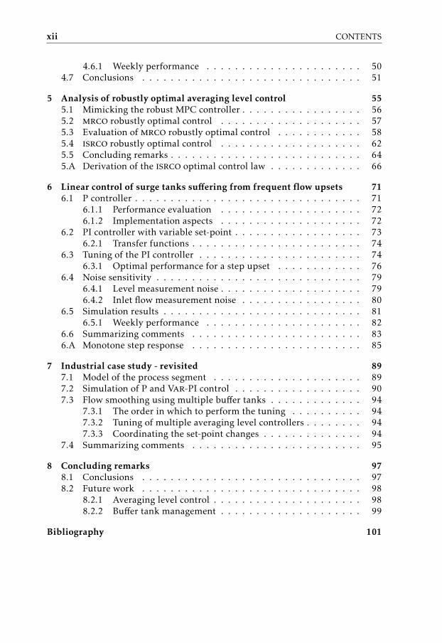
4.6.1 Weekly performance . . . . . . . . . . . . . . . . . . . . . . 504.7 Conclusions . . . . . . . . . . . . . . . . . . . . . . . . . . . . . . . 51
5 Analysis of robustly optimal averaging level control 555.1 Mimicking the robust MPC controller . . . . . . . . . . . . . . . . . 565.2 mrco robustly optimal control . . . . . . . . . . . . . . . . . . . . 575.3 Evaluation of mrco robustly optimal control . . . . . . . . . . . . 585.4 isrco robustly optimal control . . . . . . . . . . . . . . . . . . . . 625.5 Concluding remarks . . . . . . . . . . . . . . . . . . . . . . . . . . . 645.A Derivation of the isrco optimal control law . . . . . . . . . . . . . 66
6 Linear control of surge tanks suffering from frequent flow upsets 716.1 P controller . . . . . . . . . . . . . . . . . . . . . . . . . . . . . . . . 71
6.1.1 Performance evaluation . . . . . . . . . . . . . . . . . . . . 726.1.2 Implementation aspects . . . . . . . . . . . . . . . . . . . . 72
6.2 PI controller with variable set-point . . . . . . . . . . . . . . . . . . 736.2.1 Transfer functions . . . . . . . . . . . . . . . . . . . . . . . . 74
6.3 Tuning of the PI controller . . . . . . . . . . . . . . . . . . . . . . . 746.3.1 Optimal performance for a step upset . . . . . . . . . . . . 76
6.4 Noise sensitivity . . . . . . . . . . . . . . . . . . . . . . . . . . . . . 796.4.1 Level measurement noise . . . . . . . . . . . . . . . . . . . . 796.4.2 Inlet flow measurement noise . . . . . . . . . . . . . . . . . 80
6.5 Simulation results . . . . . . . . . . . . . . . . . . . . . . . . . . . . 816.5.1 Weekly performance . . . . . . . . . . . . . . . . . . . . . . 82
6.6 Summarizing comments . . . . . . . . . . . . . . . . . . . . . . . . 836.A Monotone step response . . . . . . . . . . . . . . . . . . . . . . . . 85
7 Industrial case study - revisited 897.1 Model of the process segment . . . . . . . . . . . . . . . . . . . . . 897.2 Simulation of P and Var-PI control . . . . . . . . . . . . . . . . . . 907.3 Flow smoothing using multiple buffer tanks . . . . . . . . . . . . . 94
7.3.1 The order in which to perform the tuning . . . . . . . . . . 947.3.2 Tuning of multiple averaging level controllers . . . . . . . . 947.3.3 Coordinating the set-point changes . . . . . . . . . . . . . . 94
7.4 Summarizing comments . . . . . . . . . . . . . . . . . . . . . . . . 95
8 Concluding remarks 978.1 Conclusions . . . . . . . . . . . . . . . . . . . . . . . . . . . . . . . 978.2 Future work . . . . . . . . . . . . . . . . . . . . . . . . . . . . . . . 98
8.2.1 Averaging level control . . . . . . . . . . . . . . . . . . . . . 988.2.2 Buffer tank management . . . . . . . . . . . . . . . . . . . . 99
Bibliography 101
Notation
Abbreviations
Abbreviation Meaning
mrco Maximum rate of change of the outlet flowisrco Integrated squared rate of change of the outlet flowMPC Model predictive control
P Proportional (controller)PI Proportional integral (controller)
Fix-PI PI controller with fixed set-pointVar-PI PI controller whose set-point is variedDCS Distributed control system
Miscellaneous
Notation Meaning
x(t) Continuous-time variable xx(k) Discrete-time variable xX(s) Laplace transform of x(t)x(t) Derivative of x(t) with respect to time∆x(k) Discrete-time difference, 1
Ts(x(k) − x(k − 1))
||x||∞ maxt |x(t)|||x||22
∫∞0 x(t)2dt
||∆x||∞ maxk |∆x(k)|||∆x||22 Ts
∑∞0 |∆x(k)|2
X A setTs Sampling interval for discrete-time formulations· T TransposeJ Objective function of an optimization problemx∗ Optimal value of x for minx J(x)<x Real part of x=x Imaginary part of x
xiii
xiv Notation
System Description
Notation Meaning
y Tank levelqin Inlet flow to the tank
qout, u Outlet flow from the tank, the control signalkv Parameter relating percental flow imbalance to per-
cental change of tank levelymin, ymax Lower and upper limit for the tank levelqmin, qmax Lower and upper limit for the inlet and outlet flows
Linear Control
Notation Meaning
Kc, TI Parameters describing the PI controllerKp, bp, bp Parameters describing the P controllerKSP , bSP Parameters describing the affine map
r Set-point of the tank levelAmax Largest anticipated inlet flow upsetydev Largest desired deviation in tank levelu0 Desired value of u(0)−p Pole of a system−z Zero of a systemζ Relative damping
Model Predictive Control
Notation Meaning
M Matrix operating over the whole prediction horizonx Vector of x(k) for the whole prediction horizon1 Vector of onesI Unity matrixN Prediction horizon of the MPC formulation
Optimal Control
Notation Meaning
q0, y0, u0 Initial valuesq1, y1 Final valuesT Time to cancel out flow imbalanceH Hamiltonian
1Introduction
Within the process industry, buffer tanks are used for many purposes. For exam-ple, to store the final product to ensure quick responses to customer orders oras intermediate storages allowing for partial production although some part of afactory is stopped. The application considered in this thesis is the use of buffertanks as a mean to average out flow variations. Abrupt changes to the throughputflow risk upsetting the processes, thus affecting the quality of the actual product.By using buffer tanks, up- and downstream flows are decoupled and the propa-gation of flow variations mitigated.
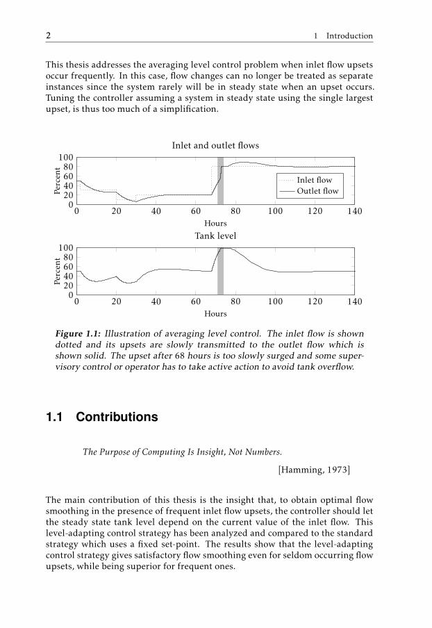
Ideally, the buffer tank functions as a low pass, preventing upstream flow varia-tions from upsetting the downstream processes. Following an inlet flow change,flow smoothing has traditionally been obtained by letting the tank level deviatefrom its nominal value while the outlet flow is slowly adjusted to cancel out theflow imbalance as illustrated in Figure 1.1. The tank level is then brought backto its set-point and the system is ready to surge the next upset. The outlet can,however, not be adjusted too slowly to the new throughput, since the situationin the shaded part of Figure 1.1 then might occur. The nominally used controlaction is too slow and a supervisory controller, e.g., an operator, ultimately needsto take rapid actions to prevent the tank from overflowing. In that case, the out-let flow has to be very abruptly changed and the whole purpose of the tank iscounteracted.
For seldom occurring flow changes, the situation in the shaded part of Figure 1.1can, however, easily be avoided. Since the system will be in, or at least suffi-ciently close to, steady state at the time of an upset, flow changes can be treatedas separate events. By ensuring that the controller is designed and tuned to han-dle the single largest flow change, the surge tank will smooth any upstream flowvariations before they are transmitted to the downstream processes.
1
2 1 Introduction
This thesis addresses the averaging level control problem when inlet flow upsetsoccur frequently. In this case, flow changes can no longer be treated as separateinstances since the system rarely will be in steady state when an upset occurs.Tuning the controller assuming a system in steady state using the single largestupset, is thus too much of a simplification.
0 20 40 60 80 100 120 1400
20406080
100
Hours
Perc
ent
Inlet and outlet flows
Inlet flowOutlet flow
0 20 40 60 80 100 120 1400
20406080
100
Hours
Perc
ent
Tank level
Figure 1.1: Illustration of averaging level control. The inlet flow is showndotted and its upsets are slowly transmitted to the outlet flow which isshown solid. The upset after 68 hours is too slowly surged and some super-visory control or operator has to take active action to avoid tank overflow.
1.1 Contributions
The Purpose of Computing Is Insight, Not Numbers.
[Hamming, 1973]
The main contribution of this thesis is the insight that, to obtain optimal flowsmoothing in the presence of frequent inlet flow upsets, the controller should letthe steady state tank level depend on the current value of the inlet flow. Thislevel-adapting control strategy has been analyzed and compared to the standardstrategy which uses a fixed set-point. The results show that the level-adaptingcontrol strategy gives satisfactory flow smoothing even for seldom occurring flowupsets, while being superior for frequent ones.
1.2 Thesis outline 3
The results presented in this thesis have to some extent previously been pub-lished in
P. Rosander, A.J. Isaksson, J. Löfberg, and K. Forsman. Robust averag-ing level control. In Proccedings of the 2011 AIChE Annual Meeting,Minneapolis,USA, 2011.
P. Rosander, A.J. Isaksson, J. Löfberg, and K. Forsman. Performaceanalysis of robust averaging level control. In Proceedings of ChemicalProcess Control VIII, Savannah, USA, 2012a.
P. Rosander, A.J. Isaksson, J. Löfberg, and K. Forsman. Practical con-trol of surge tanks suffering from frequent inlet flow upsets. In Pro-ceedings of the IFAC Conference on Advances in PID Control, Brescia,ITA, 2012b.
1.2 Thesis outline
The thesis is organized as follows
Chapter 2 describes the averaging level control problem and previous contribu-tions to the area are reviewed.
Chapter 3 presents the Perstorp problem which initiated this work and serves asthe thought of application for the conducted research. Also the difficultiesthat the previous contributions face for this application are illustrated.
Chapter 4 gives a short introduction to robust MPC and then uses it as an in-strument to obtain a controller that achieves good flow smoothing for afrequently changing inlet flow.
Chapter 5 analyzes the level-adapting property that the robust MPC exhibitsby heuristically mimicking the robust MPC using optimal non-linear con-trollers.
Chapter 6 discusses linear controllers that mimic the robust MPC but have largerindustrial applicability.
Chapter 7 revisits the Perstorp application and briefly discusses the flow smooth-ing problem when multiple tanks are considered.
Chapter 8 concludes the thesis and discusses possible future work.

2Averaging level control
Surge tanks are used in the process industry to prevent upstream flow variationsfrom upsetting downstream processes. Ideally, the tank should function as alow pass filter such that when the inlet flow changes, the capacity of the tank isused to slowly adjust the outlet flow to the new throughput. There are, however,constraints on the system, such as limited tank and flow capacity that one has toconsider when designing the level controller for a surge tank.
In this chapter, the system under consideration is first described in Section 2.1.The averaging level control problem is formulated in Section 2.2. In Section 2.3some of the previously proposed controllers and control structures are presentedbefore the chapter is briefly summarized in Section 2.4.
2.1 System setup
In this thesis we consider a cylindrical buffer tank with tank level y and constantdensity liquid inlet and outlet flows qin and qout respectively. It is assumed thatthe outlet flow can be directly manipulated and to emphasize this the notationu = qout will be used. Note that this assumption holds true if the dynamics ofa possible flow controller, which is in cascade with the level controller, is suffi-ciently fast. Using mass balance we obtain the continuous time model
y(t) = kv (qin(t) − u(t)) , (2.1)
where all quantities are assumed to be given in percent except for kv which hasthe unit h−1. The system parameter kv thus describes how one percent of flowimbalance affects the percental change in tank level per time unit, which in thisthesis is hours. Another way to put it, is that kv is the inverse of the filling time
5
6 2 Averaging level control
of the tank when u(t) = 0 % and the inlet flow is kept constant at qin = 100 %.There are also constraints on the system, such as limited tank and flow capacity
ymin ≤ y ≤ ymax, (2.2a)
qmin ≤ qin, u ≤ qmax. (2.2b)
If no extra safety limitations are put on the level, ymin = 0 % and ymax = 100 %.When it comes to the flow limitations, there is typically some lower limit on thethroughput for the downstream processes to function properly. Flows less thanthis lower limit require that downstream processes are either stopped or that flowis maintained by some sort of recirculation. In this thesis, these considerationsare disregarded and thus qmin = 0 % and qmax = 100 % will be used as flow limitsin, e.g., simulations and numerical examples, unless stated otherwise. Further-more, it is also assumed that the inlet and outlet flow have equal range, (2.2b).This guarantees that we do not risk facing a situation where violating the levelconstraints is inevitable due to lack of outlet flow capacity. In practice the outletflow could have greater range than the inlet flow, but for the derivations and re-sults presented in this thesis that would mainly complicate the notation. For thesame reason we assume that the inlet flow is directly measurable. In any case, thelinear dynamics of the system allow for a straightforward estimation of the inletflow using, e.g., the Kalman filter as shown in [Khanbaghi et al., 2001].
2.2 Mathematical problem formulation
The objective of an averaging level controller is to smooth out any inlet flow up-sets, i.e., that u should be kept “small”. How well a controller achieves this istypically quantified by either the integrated squared rate of change of the outletflow, the isrco,
||u||22 =
∞∫0
u(t)2 dt, (2.3)
or the maximum rate of change of the outlet flow, the mrco,
||u||∞ = maxt|u(t)|. (2.4)
Note that the integral in (2.3) does not need to exist as it might diverge. Froma mathematical viewpoint (if the Riemann integral is used) it also permits u tohave finitely many jump discontinuities. Such behavior is of course not desirablebut it allows the outlet to be non-differentiable at the time instant of an inlet flowstep. The mrco on the other hand requires u to be differentiable. To permit u tobe jump discontinuous and still measure the largest flow change we will use thesame criterion as in [McDonald et al., 1986]
supt,t′>0, t,t′
∣∣∣∣∣u(t) − u(t′)t − t′
∣∣∣∣∣ . (2.5)
2.2 Mathematical problem formulation 7
If u exists, (2.4) and (2.5) coincide and in the sequel the latter will be referred toas the mrco.
Under the assumption that the inlet and outlet flows are, or are approximatedwell enough as, constant during a sampling time of length Ts, the discrete-timemodel of (2.1) is given by1
y(k + 1) = y(k) + kvTs (qin(k) − u(k)) . (2.6)
The performance can then be measured using (2.4)
||∆u||22 =1Ts
∞∑k=0
|u(k) − u(k − 1)|2, (2.7)
||∆u||∞ = maxk
1Ts|u(k) − u(k − 1)|, k = 0, 1, . . . (2.8)
In previous contributions, either one of the mrco or isrco have been used, andwhich criterion that best captures “good flow filtering” is not obvious and typ-ically depends on the nature of the downstream processes. In this thesis, boththe mrco and isrco will be used to quantify filtering performance. Admittedly,they do not provide the full picture, but used together they are still quite relevantsince they measure different properties of the outlet flow. The isrco captures thewhole transient, with the drawback that even slow changes of u (i.e., u small)affect the criterion, although they rarely cause any problem for downstream pro-cesses. The drawback with the mrco is the opposite, since it is only concernedwith the largest change of u, it disregards a lot of information on how the outletflow adapts to the new throughput.
A mathematical formulation of an averaging level control problem typically in-volves minimization of either the isrco or the mrco or some related quantity2
subject to
• the process dynamics, (2.1),
• an assumption on the nature of qin,
• constraints ensuring that the level stays within its bounds (for the givenassumption on the inlet flow),
• and some assumption on how the outlet flow is controlled.
Let us illustrate this with an example.
1Strictly speaking y(k) should be replaced with y(kTs).2The derivations can sometimes be greatly simplified by not using the exact formulation of the
mrco or isrco.
8 2 Averaging level control
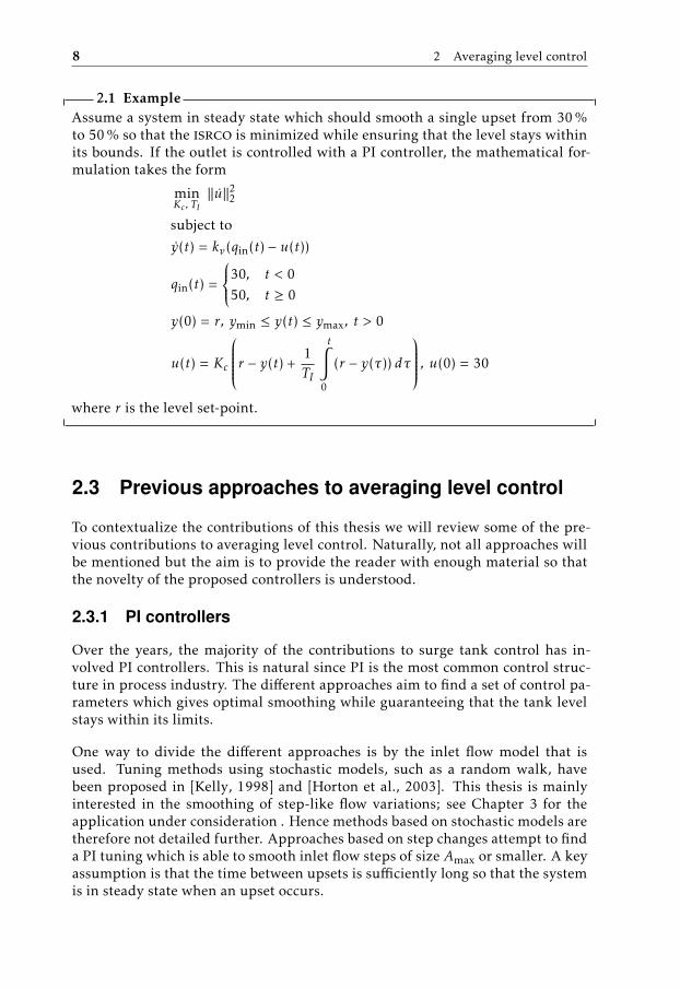
2.1 ExampleAssume a system in steady state which should smooth a single upset from 30 %to 50 % so that the isrco is minimized while ensuring that the level stays withinits bounds. If the outlet is controlled with a PI controller, the mathematical for-mulation takes the form
minKc , TI
||u||22
subject to
y(t) = kv(qin(t) − u(t))
qin(t) =
30, t < 050, t ≥ 0
y(0) = r, ymin ≤ y(t) ≤ ymax, t > 0
u(t) = Kc
r − y(t) +1TI
t∫0
(r − y(τ)) dτ
, u(0) = 30
where r is the level set-point.
2.3 Previous approaches to averaging level control
To contextualize the contributions of this thesis we will review some of the pre-vious contributions to averaging level control. Naturally, not all approaches willbe mentioned but the aim is to provide the reader with enough material so thatthe novelty of the proposed controllers is understood.
2.3.1 PI controllers
Over the years, the majority of the contributions to surge tank control has in-volved PI controllers. This is natural since PI is the most common control struc-ture in process industry. The different approaches aim to find a set of control pa-rameters which gives optimal smoothing while guaranteeing that the tank levelstays within its limits.
One way to divide the different approaches is by the inlet flow model that isused. Tuning methods using stochastic models, such as a random walk, havebeen proposed in [Kelly, 1998] and [Horton et al., 2003]. This thesis is mainlyinterested in the smoothing of step-like flow variations; see Chapter 3 for theapplication under consideration . Hence methods based on stochastic models aretherefore not detailed further. Approaches based on step changes attempt to finda PI tuning which is able to smooth inlet flow steps of size Amax or smaller. A keyassumption is that the time between upsets is sufficiently long so that the systemis in steady state when an upset occurs.
2.3 Previous approaches to averaging level control 9
In this thesis, the ideal form of the PI controller will be used
u(t) = Kc
r − y(t) +1TI
t∫0
(r − y(τ)) dτ
(2.9)
where r is the set-point. Taking the Laplace transform of (2.1) and (2.9) the equa-tions describing the closed loop system can be derived as
U (s) =−Kckv
(s + 1
TI
)(s + p1)(s + p2)
Qin(s) +Kcs
(s + 1
TI
)(s + p1)(s + p2)
R(s),
Y (s) =kvs
(s + p1)(s + p2)Qin(s) +
−Kckv(s + 1
TI
)(s + p1)(s + p2)
R(s),
(2.10)
where U (s), Qin(s), Y (s) and R(s) are the Laplace transform of u(t), qin(t), y(t)and r(t) respectively. The poles, −p1 and −p2, are given by
−p1,−p2 =kvKcTI ±
√k2vK
2c T
2I + 4kvKcTI
2TI. (2.11)
The oscillativity of the step responses of these second order systems is indicatedby the value of the relative damping, ζ,
ζ = cos(tan−1
(∣∣∣∣∣=(p1)<(p1)
∣∣∣∣∣)) . (2.12)
Here = and < denote the imaginary and real part of p1 respectively. Forcomplex-valued poles, ζ < 1 and the lower the value of ζ, the more oscillativewill the step response be.
In [Cheung and Luyben, 1979a] tuning guidelines on the selection of Kc and TIto achieve optimal flow filtering were presented. Given that the user specifies thelargest anticipated change of the inlet flow Amax, the maximum deviation (fromthe nominal value r) in tank level ydev and the initial rate of change of the out-let flow u0, the PI parameters fulfilling the specification is found. For a relativedamping greater than 0.5 the mrco is obtained at t = 0 and thus equals3 thespecified value u0, [Lee and Shin, 2009]. Optimal flow smoothing can hence beobtained by iteratively decreasing the value of u0 while checking that the result-ing values of Kc and TI give ζ ≥ 0.5.
Given a specification, the problem of finding Kc and TI neatly separates into twosub-problems. First Kc is chosen to fulfill the performance requirements usingthe relation
u(0) = u0⇔KckvAmax = u0 (2.13)
3Otherwise the mrco is larger than u0.
10 2 Averaging level control
and then TI is selected to maintain feasibility using
tpeak =ln
(p2p1
)p2 − p1
, (2.14a)
ydev ≥ Amaxkve−αtpeak
2 sin(tpeak
√β − α2/4
)√β − α2/4
, (2.14b)
where α = −kvKc, β = − kvKcTIand tpeak is the time when the tank level attains its
largest value. There does not exist an explicit solution to (2.14) and one must thusresort to numerical solutions. The tuning obtained using these rules is illustratedin the example below.
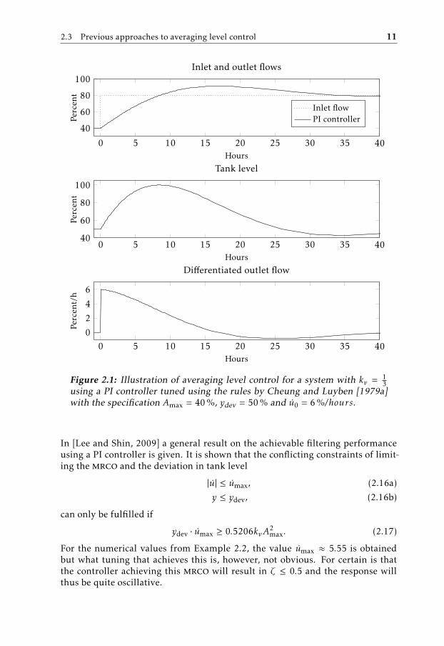
2.2 ExampleAssume a system with filling time of 3 hours (yielding kv = 1
3 ) and that upsetsup to the size Amax = 40 % should be handled. If we assume that the set-point isr = 50 %, the maximum permitted deviation in tank level is ydev = 50 %. Opti-mal filtering is then obtained by specifying u0 as small as possible while checkingthat ζ ≥ 0.5. In this case u0 = 6 %/h gives the relative damping 0.53. With thisspecification it follows using (2.13) that Kc = −0.45. Inserting this into (2.14)gives TI = 7.56 h−1. The averaging of an upset from 40 % to 80 % for the calcu-lated controller is shown in Figure 2.1, where we see that the tank level reachesits maximum (as desired when using ydev = 50) before it starts returning to r.The settling time of the system also becomes quite long and a more conservativespecification would probably be necessary in a real-life situation.
Note that typically ydev is not selected to equal |ymax − r | or |ymin − r | since onewants to add some robustness towards uncertainty in the design, for examplethat the system is not in steady state when an upset occurs.
Another approach that also considers the tuning of PI controllers to achievesmoothing of step upsets is [Shin et al., 2008]. Similarly to the previous one,the user specifies the largest anticipated upset Amax and given constraints on u,the decay ratio4 and the relative damping of the system, the PI parameters whichminimize a weighted objective of tank level and outlet flow variations
minω
∞∫0
(y(t)
ymax − ymin
)2
dt + (1 − ω)
∞∫0
(u(t)umax
)2
dt (2.15)
are found. The parameter umax is the constraint on u, thus |u| ≤ umax. This tuningapproach was later extended in [Lee and Shin, 2009] where the constraints onthe decay ratio and the relative damping was replaced with a constraint on thepermitted maximum deviation in tank level. An advantage with this approach isthat it provides the user with the possibility to compromise between the mrcoand the isrco.
4The rate between consecutive local maximum of the step response.
2.3 Previous approaches to averaging level control 11
0 5 10 15 20 25 30 35 4040
60
80
100
Hours
Perc
ent
Tank level
0 5 10 15 20 25 30 35 40
40
60
80
100
Hours
Perc
ent
Inlet and outlet flows
Inlet flowPI controller
0 5 10 15 20 25 30 35 400
2
4
6
Hours
Perc
ent/
h
Differentiated outlet flow
Figure 2.1: Illustration of averaging level control for a system with kv = 13
using a PI controller tuned using the rules by Cheung and Luyben [1979a]with the specification Amax = 40 %, ydev = 50 % and u0 = 6 %/hours.
In [Lee and Shin, 2009] a general result on the achievable filtering performanceusing a PI controller is given. It is shown that the conflicting constraints of limit-ing the mrco and the deviation in tank level
|u| ≤ umax, (2.16a)
y ≤ ydev, (2.16b)
can only be fulfilled if
ydev · umax ≥ 0.5206kvA2max. (2.17)
For the numerical values from Example 2.2, the value umax ≈ 5.55 is obtainedbut what tuning that achieves this is, however, not obvious. For certain is thatthe controller achieving this mrco will result in ζ ≤ 0.5 and the response willthus be quite oscillative.
12 2 Averaging level control
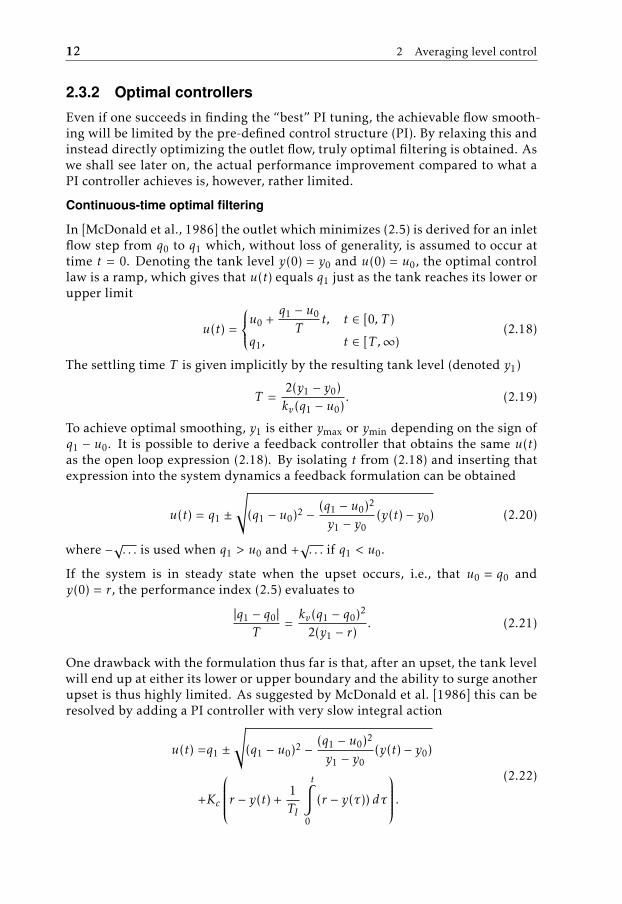
2.3.2 Optimal controllers
Even if one succeeds in finding the “best” PI tuning, the achievable flow smooth-ing will be limited by the pre-defined control structure (PI). By relaxing this andinstead directly optimizing the outlet flow, truly optimal filtering is obtained. Aswe shall see later on, the actual performance improvement compared to what aPI controller achieves is, however, rather limited.
Continuous-time optimal filtering
In [McDonald et al., 1986] the outlet which minimizes (2.5) is derived for an inletflow step from q0 to q1 which, without loss of generality, is assumed to occur attime t = 0. Denoting the tank level y(0) = y0 and u(0) = u0, the optimal controllaw is a ramp, which gives that u(t) equals q1 just as the tank reaches its lower orupper limit
u(t) =
u0 +q1 − u0
Tt, t ∈ [0, T )
q1, t ∈ [T ,∞)(2.18)
The settling time T is given implicitly by the resulting tank level (denoted y1)
T =2(y1 − y0)kv(q1 − u0)
. (2.19)
To achieve optimal smoothing, y1 is either ymax or ymin depending on the sign ofq1 − u0. It is possible to derive a feedback controller that obtains the same u(t)as the open loop expression (2.18). By isolating t from (2.18) and inserting thatexpression into the system dynamics a feedback formulation can be obtained
u(t) = q1 ±
√(q1 − u0)2 −
(q1 − u0)2
y1 − y0(y(t) − y0) (2.20)
where −√. . . is used when q1 > u0 and +√. . . if q1 < u0.
If the system is in steady state when the upset occurs, i.e., that u0 = q0 andy(0) = r, the performance index (2.5) evaluates to
|q1 − q0|T
=kv(q1 − q0)2
2(y1 − r). (2.21)
One drawback with the formulation thus far is that, after an upset, the tank levelwill end up at either its lower or upper boundary and the ability to surge anotherupset is thus highly limited. As suggested by McDonald et al. [1986] this can beresolved by adding a PI controller with very slow integral action
u(t) =q1 ±
√(q1 − u0)2 −
(q1 − u0)2
y1 − y0(y(t) − y0)
+Kc
r − y(t) +1TI
t∫0
(r − y(τ)) dτ
.(2.22)
2.3 Previous approaches to averaging level control 13
The selection of the PI parameters Kc and TI is not straightforward and the guide-lines in Section 2.3.1 are not directly applicable since the PI controller now isused in connection with the non-linear feedback controller. When adding the PIcontroller, the controller (2.22) is, of course, no longer optimal. By de-tuning thePI controller, its influence on the filtering performance can, however, be mini-mized but at the cost of a long settling time. The effect of adding a PI controlleris illustrated in the following example.
2.3 ExampleThe same setup as in Example 2.2 is assumed. The optimal controller then ob-tains the mrco 5.33, see Figure 2.2, which is quite a moderate improvementcompared to the performance value that the PI controller achieved. The tanklevel will also be at its limit following the upset. A PI controller is then addedto bring the level back to r. Doing this will worsen the flow filtering. By using ade-tuned PI (Kc = 0.01, TI = 1), it is possible to bring back the level without af-fecting the criterion significantly as themrco then evaluates to 5.6. On the otherhand the settling time of the system becomes ≈ 150 hours which is very large. Wecould try the opposite, to tune the added PI so that the system will have a settlingtime similar to what the optimal PI gives. Some manual tuning then gives thatKc = 0.05, TI = 1.1 is the tuning that worsens the criterion as little as possibleand gives a settling time of approximately 40h. The obtained mrco with thistuning is 6.4, which is actually worse than what is achieved with a standalone PIcontroller.
Discrete-time optimal filtering
The discrete-time optimal controller was presented in [Campo and Morari, 1989].The criterion is the discrete-time maximum norm (2.8) but otherwise the setup issimilar to that of the continuous-time controller. From a pedagogical perspectiveit is, however, beneficial to state the considered problem
minu(k)||∆u||∞
subject to
y(k + 1) = y(k) + Tskv (qin(k) − u(k))
qin(k) =
q0, k < 0q1, k ≥ 0
y(k) ∈ [ymin, ymax]
y(0) = y0, u(0) = u0
(2.23)
The solution to (2.23) is, just as in the continuous-time case, a ramp which evensout the flow imbalance just as the tank level reaches its boundary
u(k + 1) =
u(k) + δu , k = 1, . . . , kδ,q1, k > kδ
(2.24)
14 2 Averaging level control
0 5 10 15 20 25 30 35 40
60
80
100
Hours
Perc
ent
Tank level
0 5 10 15 20 25 30 35 4040
60
80
Hours
Perc
ent
Inlet and outlet flows
Inlet flow
Optimal
Optmimal+PI (Kc = 0.01, TI = 1)
Optmimal+PI (Kc = 0.05, TI = 1.1)
0 5 10 15 20 25 30 35 400
2
4
6
Hours
Perc
ent/
h
Differentiated outlet flow
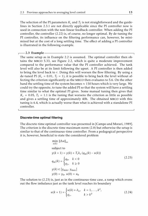
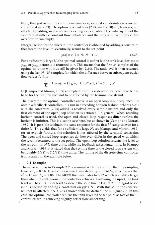
Figure 2.2: Simulation of the continuous-time optimal controller for a sys-tem with kv = 1
3 . The controller given by (2.20) is shown in solid black.The dashed black line shows its behavior when it is augmented with a PIcontroller tuned with Kc = 0.01, TI = 1. The PI brings back the level to rwithout affecting the criterion, but at the cost of a long settling time. Thedash-dotted line shows the optimal controller augmented with a PI tuned toobtain the same settling time as a standalone PI. The tuning which achievesthis and affects the performance minimally is Kc = 0.05, TI = 1.1.
where
δu =2(q1 − u0)kδ + 1
−2(y1 − y0)
kvTskδ(kδ + 1),
kδ =⌈
2(y1 − y0)kvTs(q1 − u0)
⌉.
Here demeans rounding to the smallest larger integer and y1 is again ymin or ymaxdepending on the sign of q1 − u0.
2.3 Previous approaches to averaging level control 15
Note, that just as for the continuous-time case, explicit constraints on u are notconsidered in (2.23). The optimal control laws (2.24) and (2.18) are, however, notaffected by adding such constraints as long as u can obtain the value q1. If not thesystem will suffer a constant flow imbalance and the tank will eventually eitheroverflow or run empty.
Integral action for the discrete-time controller is obtained by adding a constraintthat forces the level to, eventually, return to the set-point
y(k) = r, k = N, N + 1, . . . (2.25)
For a sufficiently largeN , the optimal control is to first let the tank level deviate toymin or ymax before it is returned to r. This means that the first kδ samples of theoptimal solution will thus still be given by (2.24). The tank level is then returnedusing the last N − kδ samples, for which the difference between subsequent outletflow values fulfills
1Ts|u(k) − u(k − 1)| ≤ δu , k = kδ + 1, kδ + 2, . . . , N .
In [Campo and Morari, 1989] an explicit formula is derived for how large N hasto be for the performance not to be affected by the terminal constraint.
The discrete-time optimal controller above is an open loop input sequence. Toobtain a feedback controller, it is run in a receding horizon fashion, where (2.23)with the constraint (2.25) added is resolved every sample instant and only thefirst element of the open loop solution is actuated. In general, when recedinghorizon control is used, the open and closed loop responses differ (unless thehorizon is infinite). This is also the case here, but as shown in [Campo and Morari,1989], it is possible to obtain the same response for the first kδ samples even for afinite N . This yields that for a sufficiently large N , see [Campo and Morari, 1989]for an explicit formula, the criterion is not affected by the terminal constraint.The open and closed loop responses do, however, differ in the speed with whichthe level is returned to the set-point. The open loop solution returns the level tothe set-point in NTs time units, while the feedback takes longer time. In [Campoand Morari, 1989] it is stated that the settling time of the closed loop system willbe roughly 2NTs to 2.5NTs time units. The tuning of the discrete-time controlleris illustrated in the example below.
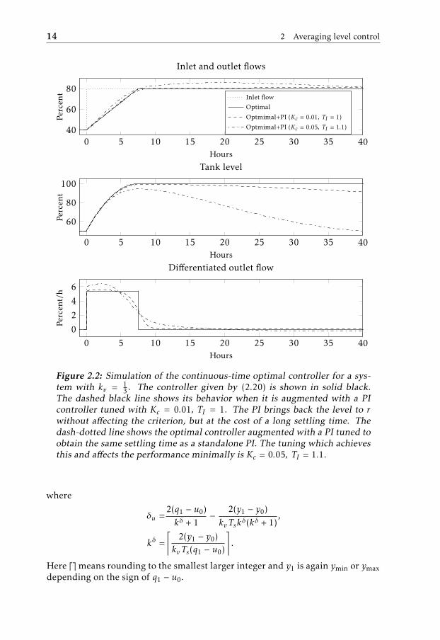
2.4 ExampleThe same setup as in Example 2.2 is assumed with the addition that the samplingtime is Ts = 0.5 h. Due to the assumed time delay, y0 = 56.67 %, which gives thatkδ = 13 and δu = 2.86. The mrco then evaluates to 5.72 which is slightly largerthan what the continuous-time controller achieves. Following the upset, the tanklevel will be at its upper level as seen in the solid line in Figure 2.3. Integral actionis thus needed by adding a constraint on y(k + N ). With this setup the criterionwill not be affected if N ≥ 28 as shown with the dashed line in Figure 2.3. In thiscase, the optimal controller returns the tank level to the set-point as fast as the PIcontroller, while achieving slightly better flow smoothing.
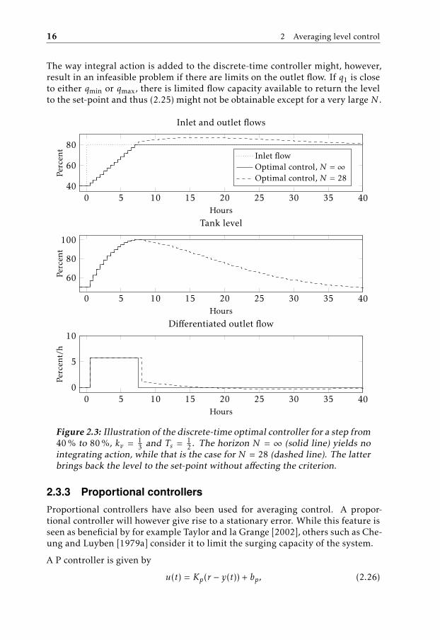
16 2 Averaging level control
The way integral action is added to the discrete-time controller might, however,result in an infeasible problem if there are limits on the outlet flow. If q1 is closeto either qmin or qmax, there is limited flow capacity available to return the levelto the set-point and thus (2.25) might not be obtainable except for a very large N .
0 5 10 15 20 25 30 35 40
60
80
100
Hours
Perc
ent
Tank level
0 5 10 15 20 25 30 35 4040
60
80
Hours
Perc
ent
Inlet and outlet flows
Inlet flowOptimal control, N = ∞Optimal control, N = 28
0 5 10 15 20 25 30 35 400
5
10
Hours
Perc
ent/
h
Differentiated outlet flow
Figure 2.3: Illustration of the discrete-time optimal controller for a step from40 % to 80 %, kv = 1
3 and Ts = 12 . The horizon N = ∞ (solid line) yields no
integrating action, while that is the case for N = 28 (dashed line). The latterbrings back the level to the set-point without affecting the criterion.
2.3.3 Proportional controllers
Proportional controllers have also been used for averaging control. A propor-tional controller will however give rise to a stationary error. While this feature isseen as beneficial by for example Taylor and la Grange [2002], others such as Che-ung and Luyben [1979a] consider it to limit the surging capacity of the system.
A P controller is given by
u(t) = Kp(r − y(t)) + bp, (2.26)
2.3 Previous approaches to averaging level control 17
where Kp is the controller gain, r the level set-point and bp a bias parameter. Theexpression can be rewritten as
u(t) = Kp(r − y(t)) + bp = −Kpy(t) + bp + Kpr︸ ︷︷ ︸bp
,
where bp is an augmented bias term, i.e., the influence of the reference is seen asa bias. For an inlet flow step change from q0 to q1 at time t = 0, the outlet flow isgiven by
u(t) = u0 + (q1 − u0)(1 − eKpkv t), (2.27)
where u0 is the value of the outlet flow at time t = 0. The isrco and mrco canthen straightforwardly be calculated
||u||22 = −(q1 − u0)2kvKp
2, (2.28a)
||u||∞ = −|q1 − u0|kvKp. (2.28b)
The minus signs come from the fact that Kp < 0 is needed for stability.
In essence, there exist two approaches to the tuning of P controllers. The earliestapproaches, see e.g., [Cheung and Luyben, 1979a], is to select the bias such thatthe nominal inlet flow value gives a desired steady state tank level (often 50 %).Kp is then selected in a similar fashion to the PI tuning so that upsets of maximumsize Amax are handled. This tuning method is illustrated in Example 2.5.
A different approach is used in [Taylor and la Grange, 2002]. The origin of thistuning is, however, unknown to the author. This tuning is based on the fact that,if the outlet flow is at its minimum value when the tank level is, the tank levelwill not decrease any further and the system will thus stay within its bounds andvice versa for the maximum tank level. This means that for the system given by(2.1) and (2.2) we want to achieve
qmin = −Kpymin + bp,
qmax = −Kpymax + bp,(2.29)
which results in the tuning
Kp = −qmax − qmin
ymax − ymin,
bp =qminymax − qmaxymin
ymax − ymin.
(2.30)
The advantage with this tuning is that the closed loop system will be feasible forall sorts of inlet flow upsets as long as the values qmin and qmax are correct. Whatparameters this tuning gives when 0 % and 100 % are the lower and upper limitis shown in the example below.
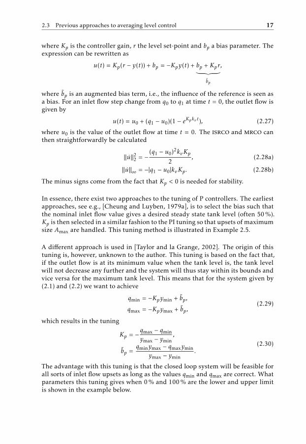
18 2 Averaging level control
2.5 ExampleThe same setup as in Example 2.2 is considered.
If it is assumed that 40 % is the nominal value and that the controller thus shouldbe able to handle upsets of Amax = 60 % or less, the tuning in [Cheung and Luy-ben, 1979a] gives the parameters Kp = −1.2 and bp = −20.
In the case of 0 % and 100 % being the limits on the tank level and flows, thetuning rule (2.30) gives Kp = −1 and bp = 0 %.
The results of these tuning methods are shown in Figure 2.4. Note that the tuning(2.30) corresponds to using 50 % as the nominal flow value and that Amax = 50 %.
0 5 10 15 20 25 30 35 4040
60
80
Hours
Perc
ent
Tank level
0 5 10 15 20 25 30 35 4040
60
80
Hours
Perc
ent
Inlet and outlet flows
Inlet flow
Kp = −1.2, bp = −20
Kp = −1, bp = 0
0 5 10 15 20 25 30 35 4005
101520
Hours
Perc
ent/
h
Differentiated outlet flow
Figure 2.4: Illustration of averaging using the P controller for a step from40 % to 80 % and kv = 1
3 .
2.4 Summarizing comments 19
2.3.4 Other averaging level controllers
Apart from the three major categories previously mentioned there exist a largevariety of other controllers and control structures. They are briefly describedbelow for completeness.
In [Luyben and Buckley, 1977] it was proposed to control the level using propor-tional feedback plus a lagged inlet flow, called PL control. This control structurewas later analyzed by Cheung and Luyben [1979b] and Ogawa [2003] where thelatter showed that the same system response can be obtained using a certain PItuning. The PL controller should thus not offer much of an improvement com-pared to a standard PI.
One way to tailor the standard P and PI controllers is to use some sort of gain-scheduling as discussed in [Shunta and Fehervari, 1976] and [Cheung and Luy-ben, 1980]. The gain Kc and possibly also the reset time TI is changed dependingon the deviation in tank level to obtain a controller that filters small upsets moresmoothly while still ensuring that also large upsets can be surged without violat-ing the level constraints. Another type of gain-scheduling is to switch between(typically two) different controllers. One variation of this is the override struc-ture which yields fast control action when the tank approaches its boundaries byswitching from a PI controller to a high gain proportional controller.
In [Wu et al., 2001], a control structure which permits designing the responses toinlet flow and reference changes separately was proposed. The controller essen-tially behaves as a PI controller and is also tuned in a similar fashion.
2.4 Summarizing comments
The dominating way to obtain averaging control is to, following an inlet flow up-set, let the tank level deviate from its set-point while slowly adapting the outletto the new throughput and eventually bringing back the tank level to its nominalset-point value. If an upset would occur during the transient, e.g., a positive upsetbetween 5 and 15 hours in Figure 2.1, very little tank volume will be available tosurge it. The flow imbalance must thus quickly be evened out to avoid overflow-ing the tank. This is typically not considered in the presented tuning methodsas they assume a system in steady state. The obvious solution to the problemthat frequent upset might cause, is to just tune the controller more tightly. Aswe shall see in Chapter 3 it is, however, not straightforward how to perform thistuning and still guarantee close to optimal filtering and that the level will staywithin its bounds. The only controller from this chapter that can easily handleupsets that occur close in time without risking violating the level constraints isthe P controller tuned according to (2.30). The drawback with the P controlleris a substantial loss in filtering performance. In the considered example, the Pcontroller achieved a mrco that was more than twice as large than for the othercontrollers.

3An industrial case study
The application that initiated the conducted research is a process segment in oneof Perstorp’s factories. Two components are first mixed in a reactor. The reactorproduct is then purified in three sequential distillation columns. There is a buffertank before each distillation column. The reactants feed vary significantly andthus upsets the whole system. The control task is to use all three surge tanks tominimize the flow variations into the final distillation column. In this chapter,this process segment will be described in some detail and we will also discusshow to tune the controllers presented in Section 2.3 for this application.
3.1 Problem setup
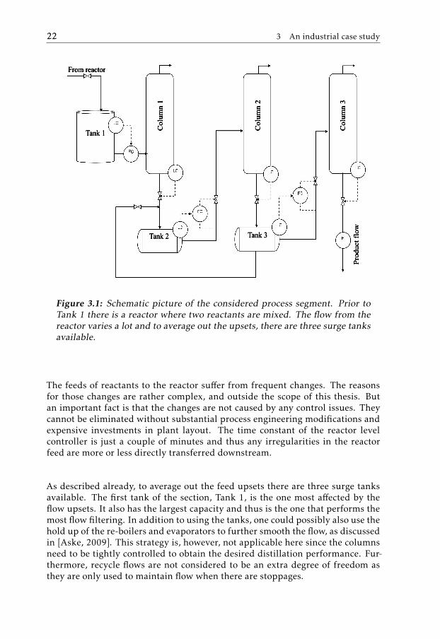
In the considered process segment, two chemical components are initially mixedin a reactor, and the resulting product is purified by three sequential distillationcolumns. Before each column there is a surge tank that is used to average out anyflow variations, see Figure 3.1. In the figure is also a recirculation pipe, that isdisregarded in this thesis shown.
The end-product from the segment is the component taken out from the bottomof the last column. As in many chemical applications, it is essential that thisbottom product does not contain any, or at least very little, of the more volatilecomponents that are taken out of the top of column. To fulfill the purity require-ments of the distillation, the flow into the column cannot fluctuate too heavily,since that would disturb the column temperature, and hence the distillate com-position. Currently, this is solved by running the column at a higher temperaturethan necessary. The column then “over-purifies” the flow entering it, with theconsequence that some of the actual product is taken out of the top.
21
22 3 An industrial case study
Tank 1
Tank 2 Tank 3
Column 1
Column 2
Column 3
From reactor
Product flow
Figure 3.1: Schematic picture of the considered process segment. Prior toTank 1 there is a reactor where two reactants are mixed. The flow from thereactor varies a lot and to average out the upsets, there are three surge tanksavailable.
The feeds of reactants to the reactor suffer from frequent changes. The reasonsfor those changes are rather complex, and outside the scope of this thesis. Butan important fact is that the changes are not caused by any control issues. Theycannot be eliminated without substantial process engineering modifications andexpensive investments in plant layout. The time constant of the reactor levelcontroller is just a couple of minutes and thus any irregularities in the reactorfeed are more or less directly transferred downstream.
As described already, to average out the feed upsets there are three surge tanksavailable. The first tank of the section, Tank 1, is the one most affected by theflow upsets. It also has the largest capacity and thus is the one that performs themost flow filtering. In addition to using the tanks, one could possibly also use thehold up of the re-boilers and evaporators to further smooth the flow, as discussedin [Aske, 2009]. This strategy is, however, not applicable here since the columnsneed to be tightly controlled to obtain the desired distillation performance. Fur-thermore, recycle flows are not considered to be an extra degree of freedom asthey are only used to maintain flow when there are stoppages.
3.2 Averaging level control for the process segment 23
0 20 40 60 80 100 120 140 1600
20406080
100
Hours
Perc
ent
Reactor feed
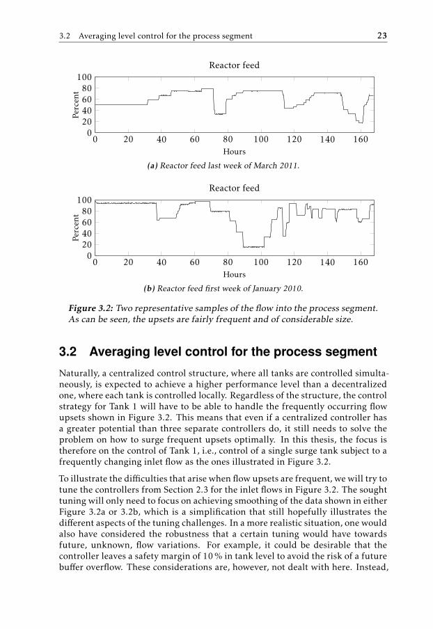
(a) Reactor feed last week of March 2011.
0 20 40 60 80 100 120 140 1600
20406080
100
Hours
Perc
ent
Reactor feed
(b) Reactor feed first week of January 2010.
Figure 3.2: Two representative samples of the flow into the process segment.As can be seen, the upsets are fairly frequent and of considerable size.
3.2 Averaging level control for the process segment
Naturally, a centralized control structure, where all tanks are controlled simulta-neously, is expected to achieve a higher performance level than a decentralizedone, where each tank is controlled locally. Regardless of the structure, the controlstrategy for Tank 1 will have to be able to handle the frequently occurring flowupsets shown in Figure 3.2. This means that even if a centralized controller hasa greater potential than three separate controllers do, it still needs to solve theproblem on how to surge frequent upsets optimally. In this thesis, the focus istherefore on the control of Tank 1, i.e., control of a single surge tank subject to afrequently changing inlet flow as the ones illustrated in Figure 3.2.
To illustrate the difficulties that arise when flow upsets are frequent, we will try totune the controllers from Section 2.3 for the inlet flows in Figure 3.2. The soughttuning will only need to focus on achieving smoothing of the data shown in eitherFigure 3.2a or 3.2b, which is a simplification that still hopefully illustrates thedifferent aspects of the tuning challenges. In a more realistic situation, one wouldalso have considered the robustness that a certain tuning would have towardsfuture, unknown, flow variations. For example, it could be desirable that thecontroller leaves a safety margin of 10 % in tank level to avoid the risk of a futurebuffer overflow. These considerations are, however, not dealt with here. Instead,
24 3 An industrial case study
we will try to find a tuning that pushes the performance of the controllers to thelimit, while keeping the system within its bounds.
The previously reviewed controllers are tuned by having the user specifying thelargest anticipated step change along with some quantity related to the desireddeviation in tank level and/or the settling time of the system. For a PI controller,such a specification can be directly transformed to control parameters, whereasthe tuning of the optimal controllers is not as obvious and requires more trialand error. They can, however, still be tuned in a similar fashion by altering the PIparameters for the continuous-time controller, and the prediction horizon for thediscrete-time controller, the level deviation and settling time of the controllersare changed. We will now try to illustrate the difficulties that arise when applyingthis tuning methodology when flow upsets are frequent. We will limit ourselvesto the tuning of PI controllers since the same or at least similar problems willarise also for the optimal non-linear controllers.
3.2.1 PI tuning
We will try to find a PI tuning for a tank with kv = 13 h−1, which is roughly the
kv of Tank 1, whose inlet flow is given by the flows in Figure 3.2. As previouslydiscussed, finding a tuning that will just keep the system feasible for a given flowrealization is by no means difficult. One just uses a controller with high gain andfairly quick integral action. A tight tuning will, however, counteract the wholepurpose of using a surge tank. The difficulty is to de-tune the controller withoutviolating any constraints as illustrated in the examples below.
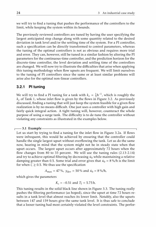
3.1 ExampleLet us start by trying to find a tuning for the inlet flow in Figure 3.2a. If flowswere infrequent, this would be achieved by ensuring that the controller couldhandle the single largest upset without overflowing the tank. Let us do the samenow, bearing in mind that the system might not be in steady state when thatupset occurs. The largest upset occurs after approximately 72 hours when theflow changes from 80 to 33 percent. We will use the tuning rules (2.13-2.14)and try to achieve optimal filtering by decreasing u0 while maintaining a relativedamping greater than 0.5. Some trial and error gives that u0 = 8 %/h is the limitfor when ζ & 0.5. We thus use the specification
Amax = 47 %, ydev = 50 % and u0 = 8 %/h,
which gives the parameters
Kc = −0.51 and TI = 5.75 h.
This tuning results in the solid black line shown in Figure 3.3. The tuning reallypushes the filtering performance (as hoped), since the upset at time 72 hours re-sults in a tank level that almost reaches its lower limit. Notably, also the upsetsbetween 147 and 159 hours give the same tank level. It is thus safe to concludethat a looser tuning had most certainly violated the level constraints. The perfor-
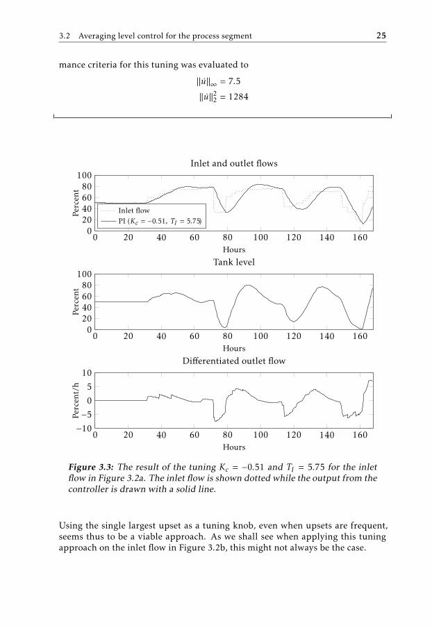
3.2 Averaging level control for the process segment 25
mance criteria for this tuning was evaluated to
||u||∞ = 7.5
||u||22 = 1284
0 20 40 60 80 100 120 140 1600
20406080
100
Hours
Perc
ent
Tank level
0 20 40 60 80 100 120 140 1600
20406080
100
Hours
Perc
ent
Inlet and outlet flows
Inlet flowPI (Kc = −0.51, TI = 5.75)
0 20 40 60 80 100 120 140 160−10
−5
0
5
10
Hours
Perc
ent/
h
Differentiated outlet flow
Figure 3.3: The result of the tuning Kc = −0.51 and TI = 5.75 for the inletflow in Figure 3.2a. The inlet flow is shown dotted while the output from thecontroller is drawn with a solid line.
Using the single largest upset as a tuning knob, even when upsets are frequent,seems thus to be a viable approach. As we shall see when applying this tuningapproach on the inlet flow in Figure 3.2b, this might not always be the case.
26 3 An industrial case study
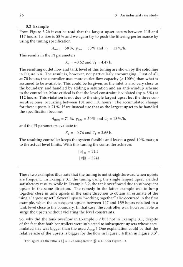
3.2 ExampleFrom Figure 3.2b it can be read that the largest upset occurs between 115 and117 hours. Its size is 58 % and we again try to push the filtering performance byusing the tuning specification
Amax = 58 %, ydev = 50 % and u0 = 12 %/h.
This results in the PI parameters
Kc = −0.62 and TI = 4.47 h.
The resulting outlet flow and tank level of this tuning are shown by the solid linein Figure 3.4. The result is, however, not particularly encouraging. First of all,at 70 hours, the controller uses more outlet flow capacity (> 100%) than what isassumed to be available. This could be forgiven, as the inlet is also very close tothe boundary, and handled by adding a saturation and an anti-windup schemeto the controller. More critical is that the level constraint is violated (by ≈ 5 %) at112 hours. This violation is not due to the single largest upset but the three con-secutive ones, occurring between 101 and 110 hours. The accumulated changefor these upsets is 71 %. If we instead use that as the largest upset to be handledthe specification becomes
Amax = 71 %, ydev = 50 % and u0 = 18 %/h,
and the PI parameters evaluate to
Kc = −0.76 and TI = 3.66 h.
The resulting controller keeps the system feasible and leaves a good 10 % marginto the actual level limits. With this tuning the controller achieves
||u||∞ = 11.5
||u||22 = 2241
These two examples illustrate that the tuning is not straightforward when upsetsare frequent. In Example 3.1 the tuning using the single largest upset yieldedsatisfactory results, while in Example 3.2, the tank overflowed due to subsequentupsets in the same direction. The remedy in the latter example was to lumptogether close in time upsets in the same direction to obtain an estimate of the“single largest upset”. Several upsets “working together” also occurred in the firstexample, when the subsequent upsets between 147 and 159 hours resulted in atank level close to the boundary. In that case, the controller was, however, able tosurge the upsets without violating the level constraints.
So, why did the tank overflow in Example 3.2 but not in Example 3.1, despiteof the fact that both controllers were subjected to subsequent upsets whose accu-mulated size was bigger than the used Amax? One explanation could be that therelative size of the upsets is bigger for the flow in Figure 3.4 than in Figure 3.31.
1For Figure 3.4 the ratio is 7158 ≈ 1.22 compared to 54
47 ≈ 1.15 for Figure 3.3.
3.2 Averaging level control for the process segment 27
This, together with the fact that the upsets in Figure 3.3 occur during a longer pe-riod of time are plausible explanations. Although these circumstances certainlyhave an influence, they do not tell the whole story. The level of the tank and thevalue of the outlet flow at the time of an upset are also important. In fact, if thesystem in Example 3.2 had been in steady state when the upsets between 101 and110 hours occurred, the controller would have been able to surge them using theinitial tuning, Kc = −0.76, TI = 3.66, without overflowing the tank, as is shownin Example 3.3.
0 20 40 60 80 100 120 140 1600
50
100
Hours
Perc
ent
Tank level
0 20 40 60 80 100 120 140 1600
50
100
Hours
Perc
ent
Inlet and outlet flows
PI (Kc = −0.62, TI = 4.47)PI (Kc = −0.76, TI = 3.66)
0 20 40 60 80 100 120 140 160−10
0
10
Hours
Perc
ent/
h
Differentiated outlet flow
Figure 3.4: The result of the PI tuning in Example 3.2. Shown with a solidline is the tuning Kc = −0.62 and TI = 4.47 while the dashed line representsthe tuning Kc = −0.76 and TI = 3.66. The former tuning is to loose as itviolates the level constraints after 112 hours.
28 3 An industrial case study
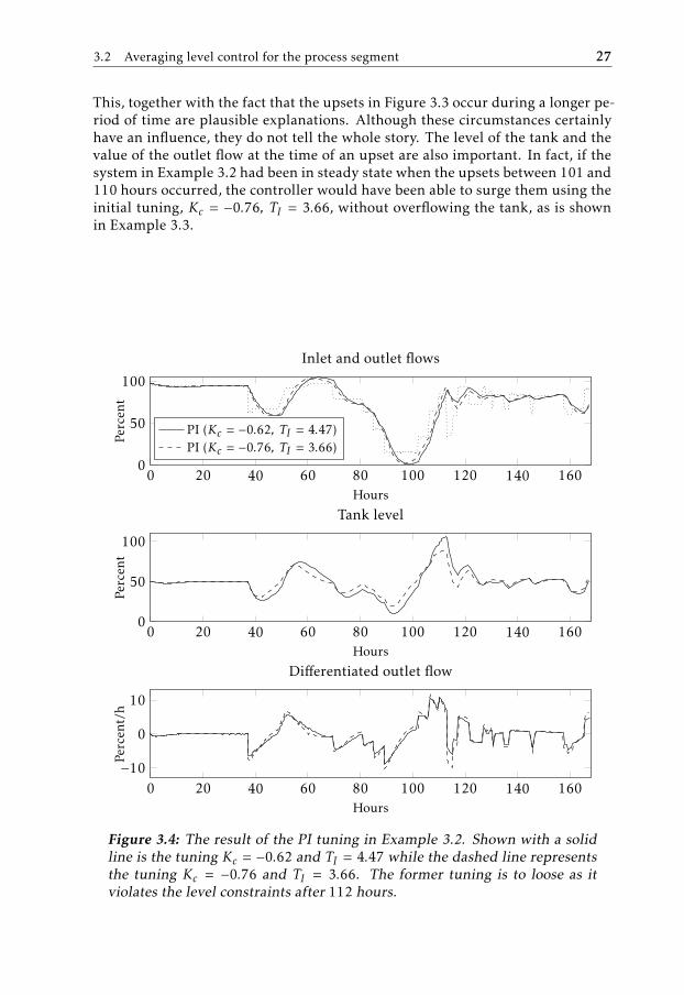
3.3 ExampleLet us review Example 3.2 and use the initial tuning
Kc = −0.62 and TI = 4.47 h.
We will now only use the data between 100 and 130 hours and assume that thesystem is initially in steady state, i.e., y(100) = 50 % and u(100) = 17 %. The be-havior of the controller is shown in Figure 3.5, where it is seen that the controllerindeed is able to surge the upsets without violating any constraints.
100 105 110 115 120 125 13040
60
80
100
Perc
ent
Tank level
100 105 110 115 120 125 1300
20406080
100
Hours
Perc
ent
Inlet and outlet flows
Inlet flowPI (Kc = −0.62, TI = 4.47)
Figure 3.5: The performance of the controller in Example 3.2 for the flowsbetween 100 and 130 assuming that the system is in steady state at time 100.The inlet flow is shown dotted and the controller data solid.
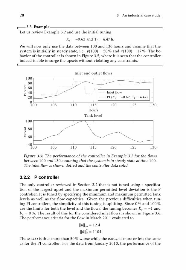
3.2.2 P controller
The only controller reviewed in Section 3.2 that is not tuned using a specifica-tion of the largest upset and the maximum permitted level deviation is the Pcontroller. It is tuned by specifying the minimum and maximum permitted tanklevels as well as the flow capacities. Given the previous difficulties when tun-ing PI controllers, the simplicity of this tuning is uplifting. Since 0 % and 100 %are the limits for both the level and the flows, the tuning becomes Kc = −1 andbp = 0 %. The result of this for the considered inlet flows is shown in Figure 3.6.The performance criteria for the flow in March 2011 evaluated to
||u||∞ = 12.4
||u||22 = 1104
Themrco is thus more than 50 % worse while the isrco is more or less the sameas for the PI controller. For the data from January 2010, the performance of the
3.3 Concluding remarks 29
0 20 40 60 80 100 120 140 1600
50
100
Hours
Perc
ent
Tank level
0 20 40 60 80 100 120 140 1600
50
100
Hours
Perc
ent
Outlet flow
March 2011Januray 2010
0 20 40 60 80 100 120 140 160−10
0
10
Hours
Perc
ent/
h
Differentiated outlet flow
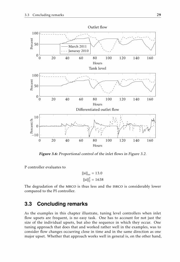
Figure 3.6: Proportional control of the inlet flows in Figure 3.2.
P controller evaluates to
||u||∞ = 13.0
||u||22 = 1638
The degradation of the mrco is thus less and the isrco is considerably lowercompared to the PI controller.
3.3 Concluding remarks
As the examples in this chapter illustrate, tuning level controllers when inletflow upsets are frequent, is no easy task. One has to account for not just thesize of the individual upsets, but also the sequence in which they occur. Onetuning approach that does that and worked rather well in the examples, was toconsider flow changes occurring close in time and in the same direction as onemajor upset. Whether that approach works well in general is, on the other hand,
30 3 An industrial case study
difficult to say. One indication that it might not, are the results from Example 3.2and 3.3, where the reason for a tank overflow in the former was an effect2 of thewhole sequence of upsets between 70 to 110 hours, rather than just the close intime upsets between 101 and 110 hours.
In a real life situation, one typically does not push the filtering performance asmuch as in the examples in this chapter. A controller that does “well enough” isoften sufficient. A real life controller must also be able to cope with future, yetunknown, flow realizations. This can be achieved by leaving some safety marginin the used tank level, i.e., using ydev 50 % when performing the tuning. Evenwith such a conservative tuning, one would probably still need to do a substantialevaluation of the controller on historical data to ensure, that the controller canindeed handle all possible scenarios.
The simple tuning of the P controller, and especially the fact that it does not re-quire upsets to be of some certain size or the system to be in steady state, makes itan attractive approach for the considered problem. The drawback with the P con-troller for infrequent upsets was a high mrco compared to other controllers, seeSection 3.2.2. For frequent upsets, this difference seems to decrease, as the othercontrol types need to be tuned tighter to avoid violating the level constraints.
2The parameters used were, admittedly, also derived using the single largest upset as Amax, in-stead of the size of the accumulated upsets.
4Model predictive control in the
presence of frequent flow upsets
As previously demonstrated in Chapter 3, frequent inlet flow changes cause prob-lems for level controllers since the fundamental assumption of a system in steadystate is violated. For a controller to achieve good filtering of frequent upsets, itcan not only focus on filtering the current upset optimally. It must also be pre-pared to handle future (yet unknown) ones. One way to obtain optimal flow filter-ing while directly accounting for future inlet flow upsets is to use robust ModelPredictive Control (MPC), as proposed here. The material which this chapter isbased on has previously been published in [Rosander et al., 2011].
The concept of MPC and robust MPC are presented in Sections 4.1 and 4.2 respec-tively. The averaging control problem is formulated in the robust MPC frame-work in Section 4.3. In Section 4.4 the tuning of the resulting controller is an-alyzed and some implementation issues are discussed. The impact of differentassumptions on the nature of the inlet flow is discussed in Section 4.5. Finally,the controller is evaluated on data from Perstorp in Section 4.6 before the chap-ter is concluded in Section 4.7.
4.1 Model predictive control
Model predictive control uses a prediction of the future response of the system tofind an optimal control signal. In every sampling instant, the current state is mea-sured and an open loop input sequence that minimizes some objective is found.The first element in that sequence is actuated and the optimization is re-run atthe next sampling instant using new state information, thus creating a feedbackloop. The field of MPC is vast and we will only present the theory relevant for ourpurposes. The interested reader is referred to, for example, [Maciejowski, 2002]
31
32 4 Model predictive control in the presence of frequent flow upsets
or [Mayne et al., 2000] for more thorough and complete descriptions.
Model predictive control for a linear time-invariant system
x(k + 1) = Fx(k) + Gu(k), (4.1)
involves, in every sample instant, solving an optimization problem that concep-tually can be written as
minuJ(x, u)
subject to
x(k + 1) = Fx(k) + Gu(k)
x(k) ∈ X, k = 1, 2, . . . , N
u(k) ∈ U, k = 0, 1, . . . , N − 1
x(0) known
(4.2)
where x(0) is the current value of the state vector and the function J(x, u) quan-tifies what the controller should achieve and X and U are the sets which thestate and input signal are constrained to. The first component, u∗(0), of an op-timal control sequence (u∗(0), u∗(1), . . . , u∗(N − 1))T is then actuated, the systemevolves, and the optimization problem is resolved when new measurement infor-mation becomes available.
The conceptual optimization problem (4.2) can be transformed into one in stan-dard form. In doing this, we will limit ourselves to the case where the sets X andU are polytopes, i.e.,
x(k) ∈ X⇔Hxx(k) ≤ mx,u(k) ∈ U⇔Huu(k) ≤ mu ,
(4.3)
for some matrices Hx and Hu and vectors mx and mu .
Before venturing forward on rewriting (4.2) into a standard optimization prob-lem, a word on the notation is needed to ease the understanding. In (4.2), x(k)and u(k) can be vectors while F and G consequently might be matrices. In thederivations we will distinguish between matrices and vectors that only act at acertain time instance and those that cover the whole prediction horizon. Vectorsthat cover the whole horizon, e.g., that consists of x and u at different time in-stances, will be denoted with a bar atop of them. Similarly, matrices that act onvectors over the whole horizon will be written in caligraphic font. To illustratethe notation, the constraint (4.3) on x(k) for the whole horizon can be written as
x ∈ X⇔Hx x ≤ mx, (4.4)
where x = (x(1), . . . , x(N ))T and
Hx =
Hx 0 . . . 00 Hx . . . 0...
. . .. . .
...0 0 . . . Hx
, mx =
mxmx...mx
.
4.2 Robust model predictive control 33
Using the dynamics of the system, it follows that
x(k) = Fkx(0) +k∑i=0
Fk−iGu(i), (4.5)
and thus that
x = F x(0) + G u, (4.6)
where, u = (u(0), . . . , u(N − 1))T, x = (x(1), . . . , x(N ))T and the matrices F and Gare built up by F and G. The linear constraints (4.4) on x can then be transformedto linear constraints on u1, as derived in [Maciejowski, 2002]. The optimizationproblem then becomes
minuJ(u)
subject to
A u ≤ b + Q x(0)
x(0) known
(4.7)
where A, b and Q depend on F , G and the matrices and vectors defining thepolytopes X and U, see [Maciejowski, 2002]. The constraints are linear and thusconvex. The convexity of the whole problem hence depends on whether the costfunction J is convex or not, [Boyd and Vandenberghe, 2004]. It thus exist plentyof alternatives, for example, either one of (2.7) and (2.8) would work as cost func-tion.
4.2 Robust model predictive control
A natural extension to (4.1) is to model that, apart from the input signal, there isalso a disturbance, w, acting on the system
x(k + 1) = Fx(k) + Gu(k) + Gww(k). (4.8)
Similarly to the undisturbed case, the constraints on u can be written as
A u + D w ≤ b + Q x(0) (4.9)
for some A, D, b and Q. There exist a number of ways to deal with the distur-bance term w. One way is to just disregard it, resulting in the optimization prob-lem (4.7). Another alternative is if w is measurable or possible to estimate. Onecould then use its last known value, w(0) or w(−1), and assume that it stays con-stant for the prediction horizon. This assumption yields the constraint
A u ≤ b + Q x(0) − D w(0). (4.10)
1Note that removing x from the optimization problem is not necessary and one could instead keepthe equality constraints (4.6) and treat x as an optimization variable. This would result in a problemwith more variables but with a sparse structure. However, such a formulation is not suitable in theuncertain case described in Section 4.2.
34 4 Model predictive control in the presence of frequent flow upsets
This approach works sufficiently well for many applications. One situation whereit risks not to, is if w varies a lot. Using the nominal value, w(0), for the wholeprediction horizon might then be too crude a simplification.
One way to deal with a varying w is to describe it as a stochastic process and treatthe constraint in a probabilistic framework. The constraint (4.9) is then guaran-teed to hold with some given probability. The drawback with this approach, asdiscussed in[Ben-Tal et al., 2009], is that the constraint (4.9) is transformed intoa non-linear and possibly non-convex constraint on u, or that one has to resort tosimulations to guarantee the constraint.
By treating w as a bounded but otherwise unknown variable, it is possible to ac-count for its influence on the system as well as obtaining linear (and thus convex)constraints on u. We will limit ourselves to deal with the case where the uncer-tainty set W is a polytope. The system is then required to stay feasible for allw ∈W
A u + D w ≤ b + Q x(0), ∀w : Hw w ≤ mw. (4.11)
In a similar fashion as in (4.6-4.7), where constraints on x were rewritten as con-straints on u, we now want to remove w from the constraints and only leave uswith either optimization variables (such as u) or constants (such as Q x(0)). Thereexist a couple of ways to perform this, as described in, for example [Löfberg,2012]. Two of those approaches will be described here: Explicit maximizationand duality a based approach.
Explicit maximization
If the polytopeW has the simple structure
wmin ≤ w ≤ wmax⇔(I−I
)w ≤
(wmax−wmin
), (4.12)
it is possible to remove the uncertainty explicitly. First a new uncertain variable,ω, which fulfills |ω| ≤ 1 is introduced. Note that ω is assumed to have the samedimension as w. The original uncertainty, w, can then be expressed in terms of ωaccordingly
w =wmax + wmin
2+ diag
wmax − wmin
2
ω = wmean + Twω (4.13)
where diag means arranging the elements of a vector along the diagonal of amatrix (denoted Tw). By introducing the matrix
Tw =
Tw 0 . . . 00 Tw . . . 0...
.... . .
...0 0 . . . Tw
the constraint (4.11) can be written as
A u + D Twω ≤ b + Q x(0) − D wmean, ∀|ω| ≤ 1. (4.14)
4.2 Robust model predictive control 35
That the above constraint holds for all ω means that it also holds for the largestvalue when optimizing over |ω| ≤ 1. The constraint (4.14) can thus be written as
max|ω|≤1
A u + D Twω ≤ b + Q x(0) − D wmean, (4.15)
where the maximum is taken row-wise. Using that max|x|≤1 P x = |P |1 where 1 is avector of ones, allows us to explicitly remove the uncertainty term ω. This givesthe robustified constraint
A u ≤ b + Q x(0) − D wmean − |D Tw | 1. (4.16)
The difference, compared to the constraint in (4.7), is that the terms −D wmeanand −|D Tw | 1 have been added to the right-hand-side of the constraint in u. Theset of feasible u has thus changed but the number of optimization variables andconstraints remain the same.
Duality based approach
For a general polytope, W , explicit maximization is not applicable, [Löfberg,2012], and we instead need to use duality theory to derive the robustified con-straints. To simplify the notation, the robust counterpart of (4.11) is derived fora single row. The full robustified constraint is then obtained by performing therobustification row-wise. For an arbitrary row the constraint reads
aTu + dTw − b − qTx(0) ≤ 0, ∀w : Hw w ≤ mw. (4.17)
Similarly to the above discussion, we can instead introduce
maxw
Jp = maxw
aTu + dTw − b − qTx(0)
subject to
Hw w ≤ mw
(4.18)
and require that its optimal value, J∗p, is less than zero. Furthermore, the optimalvalue of the dual problem of (4.18) is an upper bound2 for J∗p. If we then can finda feasible solution to the dual problem that is less than zero, we are guaranteedthat (4.17) is fulfilled. This corresponds to finding a λ such that
aTu + mTwλ ≤ b + qTx(0)
HTwλ = d
λ ≥ 0
(4.19)
Note that, in contrast to the robust constraint (4.16), auxiliary variables, λ, aswell as additional constraints have been introduced. The exact number of addedvariables and constraints depends on the structure of the polytope W , or moreexplicitly the size of Hw. Note that (4.19) is just for one row of the original con-straint, which means that the number of variables and constraints increases quite
2Since the original problem is a linear program, it follows that strong duality holds, i.e., that theoptimal value of the dual problem is indeed J∗p , [Boyd and Vandenberghe, 2004]. This holds providedthat (4.18) is feasible.
36 4 Model predictive control in the presence of frequent flow upsets
significantly compared to the explicit maximization case.
One obvious drawback with using robust optimization is thus that the size ofthe optimization problem may increase and with it, the time that it takes to findan optimal solution. The resulting controller will also be rather conservative.That this is the case, is however not obvious by just inspecting the constraints(4.16) and (4.19), though it can be understood by the fact that the controller willonly use information at the current time when it finds an optimal open loopinput sequence, u∗, that should keep the system feasible for all future possibledisturbances w. This is illustrated by applying the robustification on a simpleone-dimensional example.
4.1 ExampleLet the dynamics of the system be
x(k + 1) = x(k) + u(k) + βw(k), (4.20)
where 0 < β < 1 and x(k), u(k) andw(k) are scalars and constrained to the interval[0, 100]. If x(0) is allowed to be a free variable, the set of initial values x(0) andu(0) for which the system will stay feasible, can be investigated.
For a prediction of N = 1 the constraint on the state x(1) is
0 ≤ x(0) − u(0) + βw(0) ≤ 100, ∀w(0) ∈ [0, 100].
Explicit maximization gives the robustified constraint
0 ≤ x(0) − u(0) ≤ 100 − β · 100.
For the case of β = 13 the feasible set is drawn in Figure 4.1. Increasing the horizon
to N = 2 adds the constraint
0 ≤x(0) − u(0) + βw(0) − u(1) + βw(1) ≤ 100, ∀w ∈ [0, 100]⇔0 ≤x(0) − u(0) − u(1) ≤ 100 − β · 100 − β · 100.
(4.21)
We see that as the horizon increases the set of feasible initial points x(0) decreasesand for a horizon fulfilling
N ≥ 1β,
the upper limit of the constraint (4.21) will be negative. There will thus not existany initial x(0) for which the system will stay feasible. In the case of β = 1
3 thisoccurs already for N = 4.
4.2.1 Optimization over policies
As we saw in Example 4.1, open loop robust MPC results in a controller thatwill take conservative control actions. This is a consequence of the fact that thecontroller can only base its decision on information available at the current time,but must still keep the system feasible for all future possible disturbances w.That setup does, however, not reflect “real-life” particularly well as we know
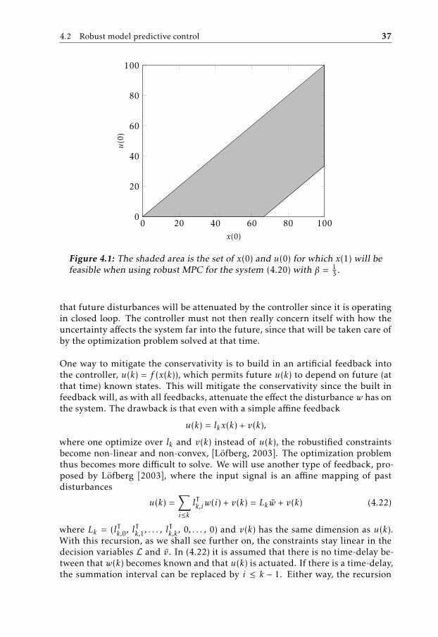
4.2 Robust model predictive control 37
0 20 40 60 80 1000
20
40
60
80
100
x(0)
u(0
)
Figure 4.1: The shaded area is the set of x(0) and u(0) for which x(1) will befeasible when using robust MPC for the system (4.20) with β = 1
3 .
that future disturbances will be attenuated by the controller since it is operatingin closed loop. The controller must not then really concern itself with how theuncertainty affects the system far into the future, since that will be taken care ofby the optimization problem solved at that time.
One way to mitigate the conservativity is to build in an artificial feedback intothe controller, u(k) = f (x(k)), which permits future u(k) to depend on future (atthat time) known states. This will mitigate the conservativity since the built infeedback will, as with all feedbacks, attenuate the effect the disturbance w has onthe system. The drawback is that even with a simple affine feedback
u(k) = lkx(k) + v(k),
where one optimize over lk and v(k) instead of u(k), the robustified constraintsbecome non-linear and non-convex, [Löfberg, 2003]. The optimization problemthus becomes more difficult to solve. We will use another type of feedback, pro-posed by Löfberg [2003], where the input signal is an affine mapping of pastdisturbances
u(k) =∑i≤k
lTk,iw(i) + v(k) = Lkw + v(k) (4.22)
where Lk = (lTk,0, lT
k,1, . . . , lT
k,k , 0, . . . , 0) and v(k) has the same dimension as u(k).With this recursion, as we shall see further on, the constraints stay linear in thedecision variables L and v. In (4.22) it is assumed that there is no time-delay be-tween that w(k) becomes known and that u(k) is actuated. If there is a time-delay,the summation interval can be replaced by i ≤ k − 1. Either way, the recursion
38 4 Model predictive control in the presence of frequent flow upsets
(4.22) can be written as u = Lw + v, where
L =
L0L1...LN
=
lT0,0 0 . . . 0lT1,0 lT1,1 . . . 0...
.... . .
...lTN,0 lTN,1 . . . lTN,N
(4.23)
where the diagonal elements had been zero if there had been a time-delay. Thenumber of optimization variables thus increases quite rapidly as it scales, approx-imately, with N2 instead of linearly as is the case if u had been optimized directly.In [Goulart et al., 2006], it was proved that the set of feasible points x(0) is thesame using (4.22) (with the summation i ≤ k − 1) as for u(k) = lkx(k) + v(k).
When using the policy (4.22), the counterpart to (4.11) becomes
(AL + D) w +A v ≤ b + Q x(0), ∀w : Hw w ≤ mw. (4.24)
Similarly to (4.16), ifW describes interval constraints, it follows that the robustcounterpart is
(AL + D) wmean +A v ≤ b + Q x(0) −Ω 1,
−Ω ≤ (AL + D)Tw ≤ Ω.(4.25)
Here we also needed to add an additional matrix-valued variable Ω to model theabsolute value of |(AL + D)Tw | (cf. with the role D Tw has in (4.16)).
IfW does not have the simple structure (4.12), we can again use the duality basedapproach. Each row of the robust constraint is then given by
aTv + mTwλ ≤ b + qTx(0)
HTwλ − aTLc = d
λ ≥ 0
(4.26)
where Lc is the column in L which corresponds to the selected row in AL.
By introducing the recursion (4.22) the size of the derived optimization prob-lem no doubt becomes larger, for example the number of optimization variablesscales with N2 (due to the introduction of L) instead of N . For the case of usingexplicit maximization to derive the robust constraints, the number of constraintsalso increases (depending on the structure of A and D) with approximately N2.However, for the duality based approach, the number of added variables andconstraints depends on the structure and size of Hw rather than on L. The com-putational cost for using the recursion (4.22) along with the duality approach isthus equal (apart for the introduction of L) as for when directly optimizing u. Al-though computationally more costly, the advantage with using the artificial feed-back (4.22) is that the conservativity of the robust MPC controller is mitigated,as is illustrated in the example below.
4.2 Robust model predictive control 39
4.2 ExampleThe same system as in Example 4.1 is considered, but now u(k) is allowed todepend on past disturbances, i.e., a time-delay between the measurement of w(k)and the actuation of u(k) is assumed.
For a prediction of N = 1 the constraint on the state x(1) is given by
0 ≤ x(0) − v(0) + βw(0) ≤ 100, ∀w(0) ∈ [0, 100],
which gives the robustified constraint
0 ≤ x(0) − v(0) ≤ 100 − β · 100.
The set of initial feasible points are thus the same as when not using the artifi-cial feedback. With the recursion, the system will however stay feasible for anarbitrary horizon. Why that is indeed the case can of course be made likely bysimulations but also realized by viewing the constraint for N = 2
0 ≤ x(0) − v(0) + βw(0) − (l1,0w(0) + v(1)) + βw(1) ≤ 100, ∀w ∈ [0, 100].
By using l1,0 = β, which is feasible since β ∈ (0, 1), the effect of w(0) on x(1) iscanceled and the robust constraint reads
0 ≤ x(0) − v(0) − v(1) ≤ 100 − β · 100,
which can be compared with (4.26). By continually using lk,k−1 = β the set offeasible initial values x(0) will stay constant3.
4.2.2 Objective function
Using the recursion (4.22) leaves a question mark on how to handle the objectivefunction, as it now contains the uncertainty
J(u) = J(Lw + v).
There, essentially, exist two ways to solve this. One way is to replace all values inw with the last known value, w(0), and thus optimize the nominal cost
minL,v
J(Lw(0) + v) (4.27)
where w(0) = (w(0), w(0), . . . , w(0))T. The requirements for that the robustifiedproblem should be convex is then that J is convex in L and v. An alternativeto minimizing the nominal cost, is to do the opposite and instead optimize theworst case cost
minL,v
maxw
J(Lw + v). (4.28)
With this formulation more restrictions than convexity need to be put on J sincewe now require that the objective function is convex after the maximization step.The maximization step in itself typically also introduce additional requirementson the nature of J for it to be possible to perform, see [Löfberg, 2012].
3This is, however, not the only option that will maintain feasibility.
40 4 Model predictive control in the presence of frequent flow upsets
Which one of (4.27) and (4.28) to use is an open ended question whose answerto a high degree depends on the application at hand. Note, however, that (4.28)typically requires more of the objective than (4.27) which only requires it to beconvex. For some applications, it might thus be much more difficult to minimizethe worst case cost.
4.3 Robust averaging level control
Generally speaking, for a controller to smooth frequent upsets well, it can notonly focus on filtering the current upset, but must also account for future ones.This can be achieved by using robust MPC. Optimal flow smoothing is achievedby using either the mrco or the isrco as objective function while robustnesstowards future upsets is obtained by treating future inlet flows as uncertain vari-ables.
The assumption of a fast varying inlet flow implies that, minimizing the worst-case scenario, i.e., (4.28), will be more representative than using the nominal cost.This rules out using the isrco since the maximization then is difficult to perform,[Löfberg, 2012]. Turning to the mrco, for a prediction horizon of length N theworst case cost is
minu
maxqin
maxk
1Ts|u(k) − u(k − 1)|, k = 0, 1, . . . , N − 1⇔
minL, v
maxqin
maxk
1Ts|(Lk − Lk−1)qin + v(k) − v(k − 1)| , k = 0, 1, . . . , N − 1
(4.29)
The optimization problem solved, in every sample instant, can thus conceptuallybe written as
minL, v
maxqin
maxk
1Ts|(Lk − Lk−1)qin + v(k) − v(k − 1)| (4.30a)
subject to
y(k + 1) = y(k) + Tskv (qin(k) − Lk qin − v(k)) (4.30b)
y(k) ∈ [ymin, ymax] ∀qin ∈ [qmin, qmax] , k = 1, 2, . . . , N (4.30c)
Lk qin + v(k) ∈ [qmin, qmax]∀qin ∈ [qmin, qmax] , k = 0, 1, . . . , N − 1 (4.30d)
y(0), qin(0), u(−1) known (4.30e)
where u(−1) is the previously actuated input, qin = (qin(1), qin(2), . . . , qin(N − 1))T,v = (v(0), v(1), . . . , v(N − 1))T and L is given by (4.23). The discrete-time dynam-ics are represented by (4.30b), where u(k) has been replaced with the artificialfeedback (4.22). The constraint (4.30d) is the constraint on the input from Sec-tion 2.1. The constraint (4.30c) guarantees that the tank level stays within itsbounds for all future values of qin. That is also the only requirement put on thetank level, i.e., it is not required that the controller brings back the level to somepredefined value (cf. the optimal controller in Section 2.4). In a sense, the con-troller is thus allowed to freely “decide” the optimal tank level, which balancesoptimal smoothing with being robust towards future flow upsets.
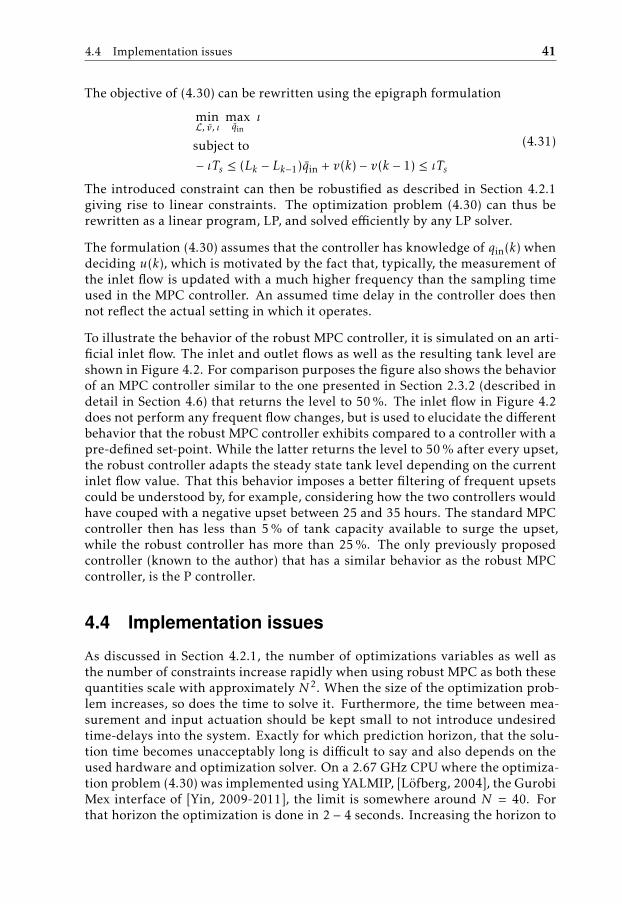
4.4 Implementation issues 41
The objective of (4.30) can be rewritten using the epigraph formulation
minL, v, ι
maxqin
ι
subject to
− ιTs ≤ (Lk − Lk−1)qin + v(k) − v(k − 1) ≤ ιTs
(4.31)
The introduced constraint can then be robustified as described in Section 4.2.1giving rise to linear constraints. The optimization problem (4.30) can thus berewritten as a linear program, LP, and solved efficiently by any LP solver.
The formulation (4.30) assumes that the controller has knowledge of qin(k) whendeciding u(k), which is motivated by the fact that, typically, the measurement ofthe inlet flow is updated with a much higher frequency than the sampling timeused in the MPC controller. An assumed time delay in the controller does thennot reflect the actual setting in which it operates.
To illustrate the behavior of the robust MPC controller, it is simulated on an arti-ficial inlet flow. The inlet and outlet flows as well as the resulting tank level areshown in Figure 4.2. For comparison purposes the figure also shows the behaviorof an MPC controller similar to the one presented in Section 2.3.2 (described indetail in Section 4.6) that returns the level to 50 %. The inlet flow in Figure 4.2does not perform any frequent flow changes, but is used to elucidate the differentbehavior that the robust MPC controller exhibits compared to a controller with apre-defined set-point. While the latter returns the level to 50 % after every upset,the robust controller adapts the steady state tank level depending on the currentinlet flow value. That this behavior imposes a better filtering of frequent upsetscould be understood by, for example, considering how the two controllers wouldhave couped with a negative upset between 25 and 35 hours. The standard MPCcontroller then has less than 5 % of tank capacity available to surge the upset,while the robust controller has more than 25 %. The only previously proposedcontroller (known to the author) that has a similar behavior as the robust MPCcontroller, is the P controller.
4.4 Implementation issues
As discussed in Section 4.2.1, the number of optimizations variables as well asthe number of constraints increase rapidly when using robust MPC as both thesequantities scale with approximately N2. When the size of the optimization prob-lem increases, so does the time to solve it. Furthermore, the time between mea-surement and input actuation should be kept small to not introduce undesiredtime-delays into the system. Exactly for which prediction horizon, that the solu-tion time becomes unacceptably long is difficult to say and also depends on theused hardware and optimization solver. On a 2.67 GHz CPU where the optimiza-tion problem (4.30) was implemented using YALMIP, [Löfberg, 2004], the GurobiMex interface of [Yin, 2009-2011], the limit is somewhere around N = 40. Forthat horizon the optimization is done in 2 − 4 seconds. Increasing the horizon to
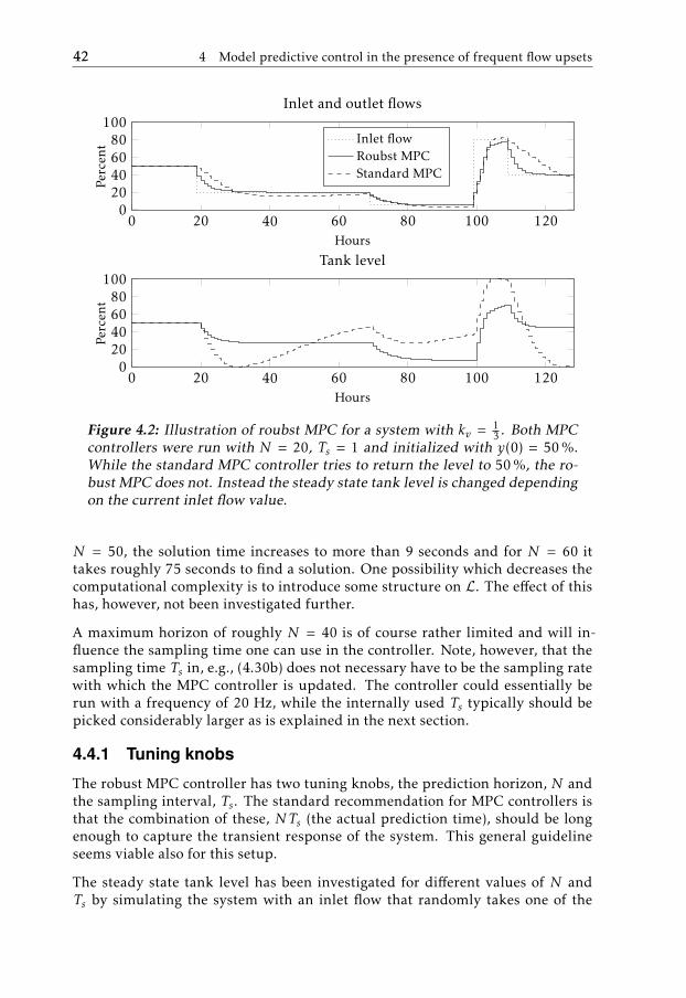
42 4 Model predictive control in the presence of frequent flow upsets
0 20 40 60 80 100 1200
20406080
100
Hours
Perc
ent
Tank level
0 20 40 60 80 100 1200
20406080
100
Hours
Perc
ent
Inlet and outlet flows
Inlet flowRoubst MPCStandard MPC
Figure 4.2: Illustration of roubst MPC for a system with kv = 13 . Both MPC
controllers were run with N = 20, Ts = 1 and initialized with y(0) = 50 %.While the standard MPC controller tries to return the level to 50 %, the ro-bust MPC does not. Instead the steady state tank level is changed dependingon the current inlet flow value.
N = 50, the solution time increases to more than 9 seconds and for N = 60 ittakes roughly 75 seconds to find a solution. One possibility which decreases thecomputational complexity is to introduce some structure on L. The effect of thishas, however, not been investigated further.
A maximum horizon of roughly N = 40 is of course rather limited and will in-fluence the sampling time one can use in the controller. Note, however, that thesampling time Ts in, e.g., (4.30b) does not necessary have to be the sampling ratewith which the MPC controller is updated. The controller could essentially berun with a frequency of 20 Hz, while the internally used Ts typically should bepicked considerably larger as is explained in the next section.
4.4.1 Tuning knobs
The robust MPC controller has two tuning knobs, the prediction horizon, N andthe sampling interval, Ts. The standard recommendation for MPC controllers isthat the combination of these, NTs (the actual prediction time), should be longenough to capture the transient response of the system. This general guidelineseems viable also for this setup.
The steady state tank level has been investigated for different values of N andTs by simulating the system with an inlet flow that randomly takes one of the
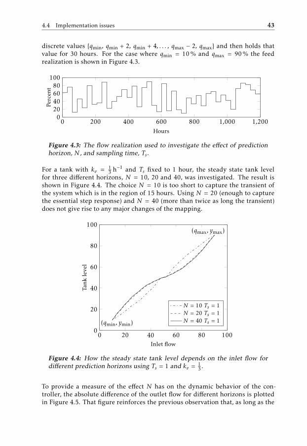
4.4 Implementation issues 43
discrete values qmin, qmin + 2, qmin + 4, . . . , qmax − 2, qmax and then holds thatvalue for 30 hours. For the case where qmin = 10 % and qmax = 90 % the feedrealization is shown in Figure 4.3.
0 200 400 600 800 1,000 1,2000
20406080
100
Hours
Perc
ent
Figure 4.3: The flow realization used to investigate the effect of predictionhorizon, N , and sampling time, Ts.
For a tank with kv = 13 h−1 and Ts fixed to 1 hour, the steady state tank level
for three different horizons, N = 10, 20 and 40, was investigated. The result isshown in Figure 4.4. The choice N = 10 is too short to capture the transient ofthe system which is in the region of 15 hours. Using N = 20 (enough to capturethe essential step response) and N = 40 (more than twice as long the transient)does not give rise to any major changes of the mapping.
(qmin, ymin)
(qmax, ymax)
0 20 40 60 80 1000
20
40
60
80
100
Inlet flow
Tank
leve
l
N = 10 Ts = 1N = 20 Ts = 1N = 40 Ts = 1
Figure 4.4: How the steady state tank level depends on the inlet flow fordifferent prediction horizons using Ts = 1 and kv = 1
3 .
To provide a measure of the effect N has on the dynamic behavior of the con-troller, the absolute difference of the outlet flow for different horizons is plottedin Figure 4.5. That figure reinforces the previous observation that, as long as the
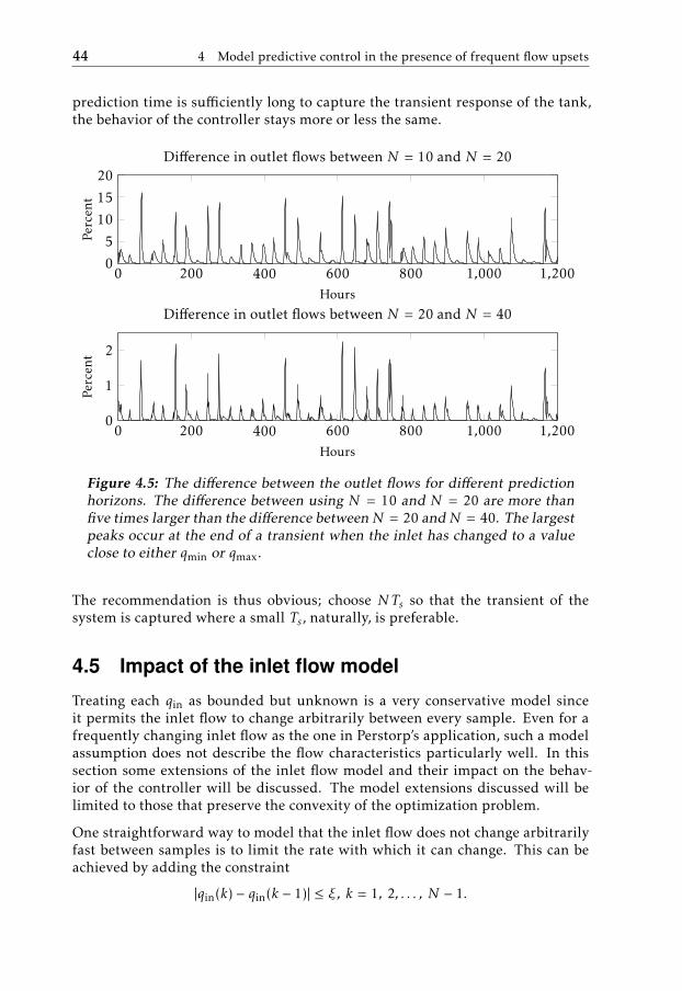
44 4 Model predictive control in the presence of frequent flow upsets
prediction time is sufficiently long to capture the transient response of the tank,the behavior of the controller stays more or less the same.
0 200 400 600 800 1,000 1,2000
5
10
15
20
Hours
Perc
ent
Difference in outlet flows between N = 10 and N = 20
0 200 400 600 800 1,000 1,2000
1
2
Hours
Perc
ent
Difference in outlet flows between N = 20 and N = 40
Figure 4.5: The difference between the outlet flows for different predictionhorizons. The difference between using N = 10 and N = 20 are more thanfive times larger than the difference between N = 20 and N = 40. The largestpeaks occur at the end of a transient when the inlet has changed to a valueclose to either qmin or qmax.
The recommendation is thus obvious; choose NTs so that the transient of thesystem is captured where a small Ts, naturally, is preferable.
4.5 Impact of the inlet flow model
Treating each qin as bounded but unknown is a very conservative model sinceit permits the inlet flow to change arbitrarily between every sample. Even for afrequently changing inlet flow as the one in Perstorp’s application, such a modelassumption does not describe the flow characteristics particularly well. In thissection some extensions of the inlet flow model and their impact on the behav-ior of the controller will be discussed. The model extensions discussed will belimited to those that preserve the convexity of the optimization problem.
One straightforward way to model that the inlet flow does not change arbitrarilyfast between samples is to limit the rate with which it can change. This can beachieved by adding the constraint
|qin(k) − qin(k − 1)| ≤ ξ, k = 1, 2, . . . , N − 1.
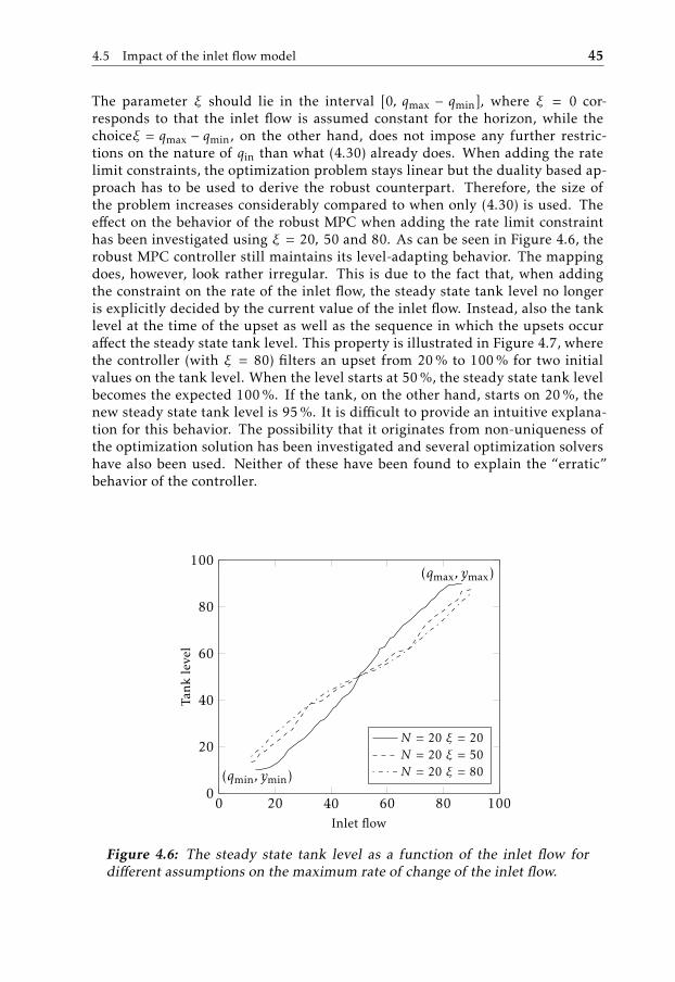
4.5 Impact of the inlet flow model 45
The parameter ξ should lie in the interval [0, qmax − qmin], where ξ = 0 cor-responds to that the inlet flow is assumed constant for the horizon, while thechoiceξ = qmax − qmin, on the other hand, does not impose any further restric-tions on the nature of qin than what (4.30) already does. When adding the ratelimit constraints, the optimization problem stays linear but the duality based ap-proach has to be used to derive the robust counterpart. Therefore, the size ofthe problem increases considerably compared to when only (4.30) is used. Theeffect on the behavior of the robust MPC when adding the rate limit constrainthas been investigated using ξ = 20, 50 and 80. As can be seen in Figure 4.6, therobust MPC controller still maintains its level-adapting behavior. The mappingdoes, however, look rather irregular. This is due to the fact that, when addingthe constraint on the rate of the inlet flow, the steady state tank level no longeris explicitly decided by the current value of the inlet flow. Instead, also the tanklevel at the time of the upset as well as the sequence in which the upsets occuraffect the steady state tank level. This property is illustrated in Figure 4.7, wherethe controller (with ξ = 80) filters an upset from 20 % to 100 % for two initialvalues on the tank level. When the level starts at 50 %, the steady state tank levelbecomes the expected 100 %. If the tank, on the other hand, starts on 20 %, thenew steady state tank level is 95 %. It is difficult to provide an intuitive explana-tion for this behavior. The possibility that it originates from non-uniqueness ofthe optimization solution has been investigated and several optimization solvershave also been used. Neither of these have been found to explain the “erratic”behavior of the controller.
(qmin, ymin)
(qmax, ymax)
0 20 40 60 80 1000
20
40
60
80
100
Inlet flow
Tank
leve
l
N = 20 ξ = 20N = 20 ξ = 50N = 20 ξ = 80
Figure 4.6: The steady state tank level as a function of the inlet flow fordifferent assumptions on the maximum rate of change of the inlet flow.
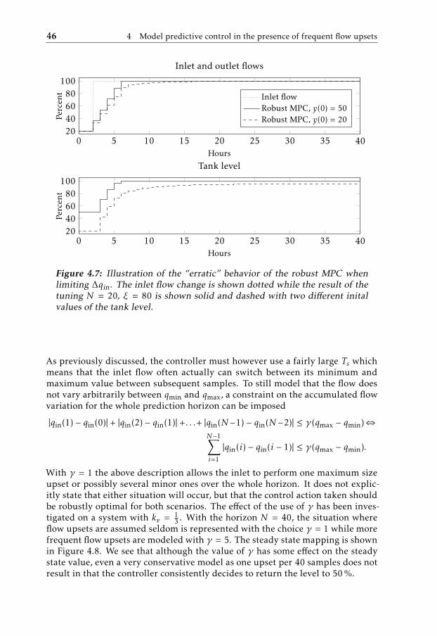
46 4 Model predictive control in the presence of frequent flow upsets
0 5 10 15 20 25 30 35 4020406080
100
Hours
Perc
ent
Inlet and outlet flows
Inlet flowRobust MPC, y(0) = 50Robust MPC, y(0) = 20
0 5 10 15 20 25 30 35 4020406080
100
Hours
Perc
ent
Tank level
Figure 4.7: Illustration of the “erratic” behavior of the robust MPC whenlimiting ∆qin. The inlet flow change is shown dotted while the result of thetuning N = 20, ξ = 80 is shown solid and dashed with two different initalvalues of the tank level.
As previously discussed, the controller must however use a fairly large Ts whichmeans that the inlet flow often actually can switch between its minimum andmaximum value between subsequent samples. To still model that the flow doesnot vary arbitrarily between qmin and qmax, a constraint on the accumulated flowvariation for the whole prediction horizon can be imposed
|qin(1) − qin(0)| + |qin(2) − qin(1)| +. . .+ |qin(N−1) − qin(N−2)| ≤ γ(qmax − qmin)⇔N−1∑i=1
|qin(i) − qin(i − 1)| ≤ γ(qmax − qmin).
With γ = 1 the above description allows the inlet to perform one maximum sizeupset or possibly several minor ones over the whole horizon. It does not explic-itly state that either situation will occur, but that the control action taken shouldbe robustly optimal for both scenarios. The effect of the use of γ has been inves-tigated on a system with kv = 1
3 . With the horizon N = 40, the situation whereflow upsets are assumed seldom is represented with the choice γ = 1 while morefrequent flow upsets are modeled with γ = 5. The steady state mapping is shownin Figure 4.8. We see that although the value of γ has some effect on the steadystate value, even a very conservative model as one upset per 40 samples does notresult in that the controller consistently decides to return the level to 50 %.
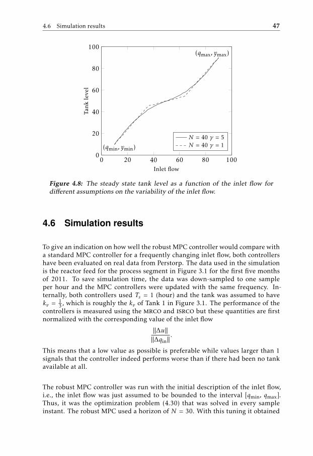
4.6 Simulation results 47
(qmin, ymin)
(qmax, ymax)
0 20 40 60 80 1000
20
40
60
80
100
Inlet flow
Tank
leve
l
N = 40 γ = 5N = 40 γ = 1
Figure 4.8: The steady state tank level as a function of the inlet flow fordifferent assumptions on the variability of the inlet flow.
4.6 Simulation results
To give an indication on how well the robust MPC controller would compare witha standard MPC controller for a frequently changing inlet flow, both controllershave been evaluated on real data from Perstorp. The data used in the simulationis the reactor feed for the process segment in Figure 3.1 for the first five monthsof 2011. To save simulation time, the data was down-sampled to one sampleper hour and the MPC controllers were updated with the same frequency. In-ternally, both controllers used Ts = 1 (hour) and the tank was assumed to havekv = 1
3 , which is roughly the kv of Tank 1 in Figure 3.1. The performance of thecontrollers is measured using the mrco and isrco but these quantities are firstnormalized with the corresponding value of the inlet flow
||∆u||||∆qin||
.
This means that a low value as possible is preferable while values larger than 1signals that the controller indeed performs worse than if there had been no tankavailable at all.
The robust MPC controller was run with the initial description of the inlet flow,i.e., the inlet flow was just assumed to be bounded to the interval [qmin, qmax].Thus, it was the optimization problem (4.30) that was solved in every sampleinstant. The robust MPC used a horizon of N = 30. With this tuning it obtained
48 4 Model predictive control in the presence of frequent flow upsets
the normalized performances
||∆u||∞||∆qin||∞
= 0.18 and||∆u||22||∆qin||22
= 0.13.
The standard MPC controller used in the evaluation is essentially the optimalcontroller proposed by Campo and Morari [1989], described in Section 2.3.2, butwith input constraints added. To avoid misconceptions, it is however restatedhere. The optimization problem solved in every sample is
minu(k)
maxk
1Ts|u(k) − u(k − 1)|
subject to
y(k + 1) = y(k) + Tskv (qin(0) − u(k))
y(k) ∈ [ymin, ymax] , k = 1, 2, . . . , N
u(k) ∈ [qmin, qmax] , k = 0, 1, . . . , N − 1
y(0), u(−1), qin(0) known
(4.32)
where u(−1) is the last actuated input signal, y(0) the current tank level and qin(0)the current value of the inlet flow. To obtain integral action the constraint
y(k + N ) = 50 (4.33)
is added, except for when the inlet flow is within 10 % of the boundary. Thecontroller then might have little flow capacity4 available to bring the level backto the set-point. This might lead to a rather sluggish behavior, where any flowimbalance is directly transferred to the outlet, or actually even to an infeasibleoptimization problem. To avoid this, the constraint (4.33) is relaxed and replacedwith a penalty term on
|y(k + N ) − 50|when the inlet is closed to its limits. The tuning of this MPC controller is a deli-cate business, since the prediction horizon determines how quickly the controllerwill return the level to the set-point and thus how aggressive the taken control ac-tion will be. One way to tune it, as discussed in Section 2.4, is to specify a typicalupset-size and a desired settling time. As we saw in Section 3.2.1, it is howeverdifficult to give such a specification when flow upsets are frequent. In this case,the horizons N = 10, 15, . . . , 35, 40, 50, . . . , 100 were all evaluated on the simu-lation data and the tuning which obtained the best performance was used in thecomparison. The presented performance values for the standard MPC are thusoptimistic estimates of what the controller would obtain in real-life.
The mrco and the isrco for the different horizons are shown in Figure 4.9. Thetuning that obtained the lowest mrco was N = 35. The reason why the mrco“saturates” for horizons larger than 40 is because all the tunings have problem
4The tank level can at most decrease with kvTs(qin(0) − qmax) and equally increase withkvTs(qin(0) − qmin).
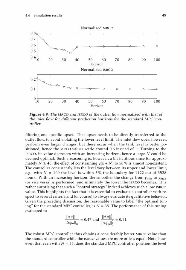
4.6 Simulation results 49
10 20 30 40 50 60 70 80 90 1000.4
0.5
0.6
0.7
0.8
Horizon
Normalized mrco
10 20 30 40 50 60 70 80 90 1000
0.1
0.2
Horizon
Normalized isrco
Figure 4.9: The mrco and isrco of the outlet flow normalized with that ofthe inlet flow for different prediction horizons for the standard MPC con-troller.
filtering one specific upset. That upset needs to be directly transferred to theoutlet flow, to avoid violating the lower level limit. The inlet flow does, however,perform even larger changes, but these occur when the tank level is better po-sitioned, hence the mrco values settle around 0.6 instead of 1. Turning to theisrco, its value decreases with an increasing horizon, hence a large N could bedeemed optimal. Such a reasoning is, however, a bit fictitious since for approxi-mately N ≥ 40, the effect of constraining y(k + N ) to 50 % is almost nonexistent.The controller consistently lets the level vary between its upper and lower limit,e.g., with N = 100 the level is within 5 % the boundary for 1122 out of 3528hours. With an increasing horizon, the smoother the change from ymin to ymax(or vice versa) is performed, and ultimately the lower the isrco becomes. It israther surprising that such a “control strategy” indeed achieves such a low isrcovalue. This highlights the fact that it is essential to evaluate a controller with re-spect to several criteria and (of course) to always evaluate its qualitative behavior.Given the preceding discussion, the reasonable value to label “the optimal tun-ing” for the standard MPC controller, is N = 35. The performance of this tuningevaluated to
||∆u||∞||∆qin||∞
= 0.47 and||∆u||22||∆qin||22
= 0.11.
The robust MPC controller thus obtains a considerably better mrco value thanthe standard controller while the isrco values are more or less equal. Note, how-ever, that even with N = 35, does the standard MPC controller position the level
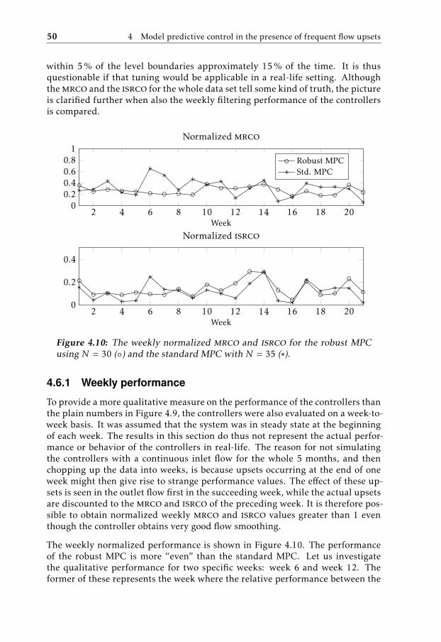
50 4 Model predictive control in the presence of frequent flow upsets
within 5 % of the level boundaries approximately 15 % of the time. It is thusquestionable if that tuning would be applicable in a real-life setting. Althoughthemrco and the isrco for the whole data set tell some kind of truth, the pictureis clarified further when also the weekly filtering performance of the controllersis compared.
2 4 6 8 10 12 14 16 18 200
0.20.40.60.8
1
Week
Normalized mrco
Robust MPCStd. MPC
2 4 6 8 10 12 14 16 18 200
0.2
0.4
Week
Normalized isrco
Figure 4.10: The weekly normalized mrco and isrco for the robust MPCusing N = 30 () and the standard MPC with N = 35 (∗).
4.6.1 Weekly performance
To provide a more qualitative measure on the performance of the controllers thanthe plain numbers in Figure 4.9, the controllers were also evaluated on a week-to-week basis. It was assumed that the system was in steady state at the beginningof each week. The results in this section do thus not represent the actual perfor-mance or behavior of the controllers in real-life. The reason for not simulatingthe controllers with a continuous inlet flow for the whole 5 months, and thenchopping up the data into weeks, is because upsets occurring at the end of oneweek might then give rise to strange performance values. The effect of these up-sets is seen in the outlet flow first in the succeeding week, while the actual upsetsare discounted to the mrco and isrco of the preceding week. It is therefore pos-sible to obtain normalized weekly mrco and isrco values greater than 1 eventhough the controller obtains very good flow smoothing.
The weekly normalized performance is shown in Figure 4.10. The performanceof the robust MPC is more “even” than the standard MPC. Let us investigatethe qualitative performance for two specific weeks: week 6 and week 12. Theformer of these represents the week where the relative performance between the
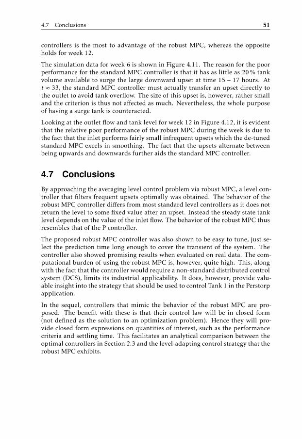
4.7 Conclusions 51
controllers is the most to advantage of the robust MPC, whereas the oppositeholds for week 12.
The simulation data for week 6 is shown in Figure 4.11. The reason for the poorperformance for the standard MPC controller is that it has as little as 20 % tankvolume available to surge the large downward upset at time 15 − 17 hours. Att ≈ 33, the standard MPC controller must actually transfer an upset directly tothe outlet to avoid tank overflow. The size of this upset is, however, rather smalland the criterion is thus not affected as much. Nevertheless, the whole purposeof having a surge tank is counteracted.
Looking at the outlet flow and tank level for week 12 in Figure 4.12, it is evidentthat the relative poor performance of the robust MPC during the week is due tothe fact that the inlet performs fairly small infrequent upsets which the de-tunedstandard MPC excels in smoothing. The fact that the upsets alternate betweenbeing upwards and downwards further aids the standard MPC controller.
4.7 Conclusions
By approaching the averaging level control problem via robust MPC, a level con-troller that filters frequent upsets optimally was obtained. The behavior of therobust MPC controller differs from most standard level controllers as it does notreturn the level to some fixed value after an upset. Instead the steady state tanklevel depends on the value of the inlet flow. The behavior of the robust MPC thusresembles that of the P controller.
The proposed robust MPC controller was also shown to be easy to tune, just se-lect the prediction time long enough to cover the transient of the system. Thecontroller also showed promising results when evaluated on real data. The com-putational burden of using the robust MPC is, however, quite high. This, alongwith the fact that the controller would require a non-standard distributed controlsystem (DCS), limits its industrial applicability. It does, however, provide valu-able insight into the strategy that should be used to control Tank 1 in the Perstorpapplication.
In the sequel, controllers that mimic the behavior of the robust MPC are pro-posed. The benefit with these is that their control law will be in closed form(not defined as the solution to an optimization problem). Hence they will pro-vide closed form expressions on quantities of interest, such as the performancecriteria and settling time. This facilitates an analytical comparison between theoptimal controllers in Section 2.3 and the level-adapting control strategy that therobust MPC exhibits.
52 4 Model predictive control in the presence of frequent flow upsets
0 20 40 60 80 100 120 140 1600
50
100
Hours
Perc
ent
Tank level
0 20 40 60 80 100 120 140 1600
50
100
Hours
Perc
ent
Inlet and outlet flows week 6
Inlet flowRobust MPCStd. MPC
0 20 40 60 80 100 120 140 160−40
−20
0
Hours
Perc
ent/
h
Differentiated outlet flow
Figure 4.11: The qualitative behavior of the controllers for week 6. The inletflow is shown dotted, the data for the robust MPC solid while the data forthe standard MPC is dashed.
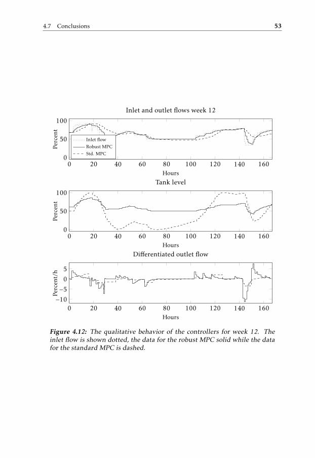
4.7 Conclusions 53
0 20 40 60 80 100 120 140 1600
50
100
Hours
Perc
ent
Tank level
0 20 40 60 80 100 120 140 1600
50
100
Hours
Perc
ent
Inlet and outlet flows week 12
Inlet flow
Robust MPC
Std. MPC
0 20 40 60 80 100 120 140 160−10
−5
0
5
Hours
Perc
ent/
h
Differentiated outlet flow
Figure 4.12: The qualitative behavior of the controllers for week 12. Theinlet flow is shown dotted, the data for the robust MPC solid while the datafor the standard MPC is dashed.

5Analysis of robustly optimal
averaging level control
The robust MPC controller provides insight into the general manner in which acontroller should achieve optimal filtering of frequent flow upsets: The tank levelshould be allowed to vary depending on the current inlet flow level instead of be-ing returned to a fixed set-point. The simulations results in the previous chaptershowed that the performance improvement using the robust MPC for frequentflow upsets could be significant. The aim of this chapter is to further analyze theproperties of the level-adapting control strategy. The behavior of the robust MPCis heuristically mimicked by imposing constraints on the tank level when deriv-ingmrco and isrco optimal control laws. These controllers provide closed formexpressions on the filtering performance as well as the settling time, while stillclosely mimicking the robust MPC. The closed form expressions facilitate an an-alytical comparison with the previously proposed non-robust optimal controllerof [McDonald et al., 1986] as well as providing lower bounds on the achievablesmoothing performance of any controller also mimicking the robust MPC. Thederived control laws are thus not the main purpose of this chapter and hence wewill limit the analysis to the situation when the system is in steady state. Some ofthe ideas and results presented in this chapter have previously been published in[Rosander et al., 2012a].
First of all the approximation that is performed to mimic the behavior of therobust MPC is presented in Section 5.1. Using this approximation, an explicitrobustly optimal control law minimizing the mrco is derived in Section 5.2. InSection 5.3, this controller is evaluated and compared with that of the truly (non-robust) optimal controller proposed by McDonald et al. [1986]. In Section 5.4,the isrco robustly optimal controller is derived. Some concluding remarks aregiven in Section 5.5.
55
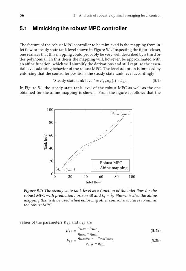
56 5 Analysis of robustly optimal averaging level control
5.1 Mimicking the robust MPC controller
The feature of the robust MPC controller to be mimicked is the mapping from in-let flow to steady state tank level shown in Figure 5.1. Inspecting the figure closer,one realizes that this mapping could probably be very well described by a third or-der polynomial. In this thesis the mapping will, however, be approximated withan affine function, which will simplify the derivations and still capture the essen-tial level-adapting behavior of the robust MPC. The level-adaption is imposed byenforcing that the controller positions the steady state tank level accordingly
"Steady state tank level" = KSP qin(t) + bSP . (5.1)
In Figure 5.1 the steady state tank level of the robust MPC as well as the oneobtained for the affine mapping is shown. From the figure it follows that the
(qmin, ymin)
(qmax, ymax)
0 20 40 60 80 1000
20
40
60
80
100
Inlet flow
Tank
leve
l
Robust MPCAffine mapping
Figure 5.1: The steady state tank level as a function of the inlet flow for therobust MPC with prediction horizon 40 and kv = 1
3 . Shown is also the affinemapping that will be used when enforcing other control structures to mimicthe robust MPC.
values of the parameters KSP and bSP are
KSP =ymax − ymin
qmax − qmin, (5.2a)
bSP =qmaxymin − qminymax
qmax − qmin. (5.2b)
5.2 mrco robustly optimal control 57
5.2 MRCO robustly optimal control
By adding the constraint (5.1) to the continuous-time optimal controller of Sec-tion 2.3, a controller that is robustly optimal in sense of the mrco, will be ob-tained. The main purpose of deriving such a controller is not the control lawitself, but rather the fact that it facilitates the possibility to perform a compari-son between the robustly and the truly (non-robust) optimal controllers.
The robustly optimal control law is derived for an arbitrary inlet flow changefrom q0 to q1 under the assumption that the system is in steady state at the timeof the upset. Without loss of generality, it is assumed that the upset occurs t = 0.The robustly optimal control law is then the solution to
minu
supt,t′>0, t,t′
∣∣∣∣∣u(t) − u(t′)t − t′
∣∣∣∣∣subject to
y(t) = kv(qin(t) − u(t))
qin(t) =
q0, t ≤ 0q1, t > 0
u(0) = q0, y0 = KSP q0 + bSPu(T ) = q1, y1 = KSP q1 + bSP ,
u(0) = u(T ) = 0
T free
(5.3)
The assumption of a system initially in steady state gives that u(0) = qin(0) andthat y(0) is positioned according to the affine mapping (5.1). From the derivationsin [McDonald et al., 1986] (and as presented in Section 2.3.2), the solution to (5.3)is
u(t) =
q0 +q1 − q0
Tt, t ∈ [0, T )
q1, t ∈ [T ,∞)(5.4)
where T is given by the flow imbalance, q1 − q0, and the initial, y0, and final, y1,tank level
T =2(y1 − y0)kv(q1 − q0)
.
Using the imposed constraints, it follows that
T =2 (KSP q1 + bSP − (KSP q0 + bSP ))
kv(q1 − q0)=
2KSPkv
. (5.5)
So for upsets occurring while in steady state, the settling time will be constant re-gardless of the size of the upset. For upsets when not in steady state, the robustlyoptimal control law is the solution to a similar optimization problem as (5.3) butwith u(0) , q0 and y0 , KSP q0 + bSP . Before venturing further with the compar-ison between the truly and robustly optimal controllers, note that the open loop
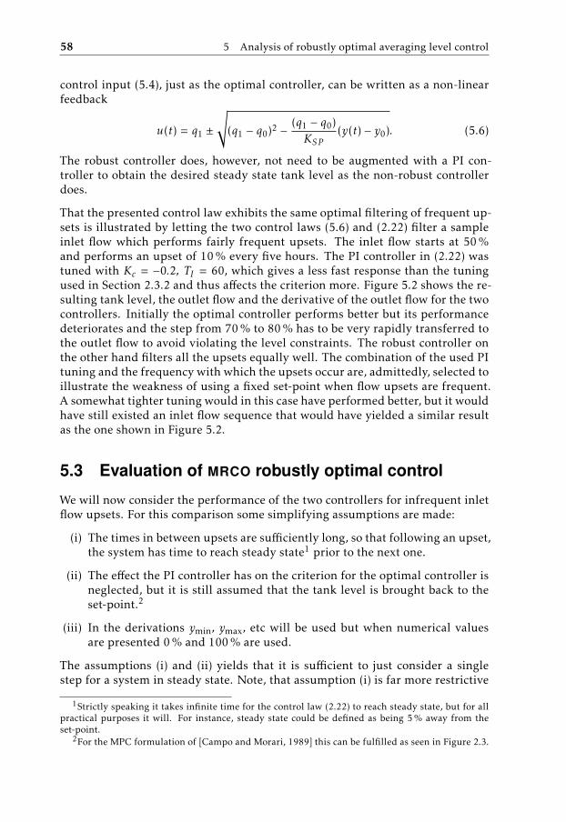
58 5 Analysis of robustly optimal averaging level control
control input (5.4), just as the optimal controller, can be written as a non-linearfeedback
u(t) = q1 ±
√(q1 − q0)2 −
(q1 − q0)KSP
(y(t) − y0). (5.6)
The robust controller does, however, not need to be augmented with a PI con-troller to obtain the desired steady state tank level as the non-robust controllerdoes.
That the presented control law exhibits the same optimal filtering of frequent up-sets is illustrated by letting the two control laws (5.6) and (2.22) filter a sampleinlet flow which performs fairly frequent upsets. The inlet flow starts at 50 %and performs an upset of 10 % every five hours. The PI controller in (2.22) wastuned with Kc = −0.2, TI = 60, which gives a less fast response than the tuningused in Section 2.3.2 and thus affects the criterion more. Figure 5.2 shows the re-sulting tank level, the outlet flow and the derivative of the outlet flow for the twocontrollers. Initially the optimal controller performs better but its performancedeteriorates and the step from 70 % to 80 % has to be very rapidly transferred tothe outlet flow to avoid violating the level constraints. The robust controller onthe other hand filters all the upsets equally well. The combination of the used PItuning and the frequency with which the upsets occur are, admittedly, selected toillustrate the weakness of using a fixed set-point when flow upsets are frequent.A somewhat tighter tuning would in this case have performed better, but it wouldhave still existed an inlet flow sequence that would have yielded a similar resultas the one shown in Figure 5.2.
5.3 Evaluation of MRCO robustly optimal control
We will now consider the performance of the two controllers for infrequent inletflow upsets. For this comparison some simplifying assumptions are made:
(i) The times in between upsets are sufficiently long, so that following an upset,the system has time to reach steady state1 prior to the next one.
(ii) The effect the PI controller has on the criterion for the optimal controller isneglected, but it is still assumed that the tank level is brought back to theset-point.2
(iii) In the derivations ymin, ymax, etc will be used but when numerical valuesare presented 0 % and 100 % are used.
The assumptions (i) and (ii) yields that it is sufficient to just consider a singlestep for a system in steady state. Note, that assumption (i) is far more restrictive
1Strictly speaking it takes infinite time for the control law (2.22) to reach steady state, but for allpractical purposes it will. For instance, steady state could be defined as being 5 % away from theset-point.
2For the MPC formulation of [Campo and Morari, 1989] this can be fulfilled as seen in Figure 2.3.
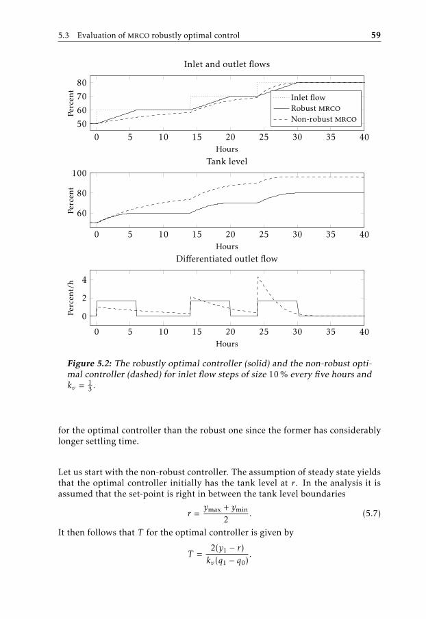
5.3 Evaluation of mrco robustly optimal control 59
0 5 10 15 20 25 30 35 40
60
80
100
Hours
Perc
ent
Tank level
0 5 10 15 20 25 30 35 4050
60
70
80
Hours
Perc
ent
Inlet and outlet flows
Inlet flowRobust mrcoNon-robust mrco
0 5 10 15 20 25 30 35 40
0
2
4
Hours
Perc
ent/
h
Differentiated outlet flow
Figure 5.2: The robustly optimal controller (solid) and the non-robust opti-mal controller (dashed) for inlet flow steps of size 10 % every five hours andkv = 1
3 .
for the optimal controller than the robust one since the former has considerablylonger settling time.
Let us start with the non-robust controller. The assumption of steady state yieldsthat the optimal controller initially has the tank level at r. In the analysis it isassumed that the set-point is right in between the tank level boundaries
r =ymax + ymin
2. (5.7)
It then follows that T for the optimal controller is given by
T =2(y1 − r)kv(q1 − q0)
.
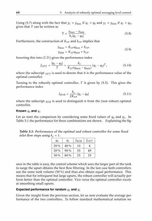
60 5 Analysis of robustly optimal averaging level control
Using (5.7) along with the fact that y1 = ymax if q1 > q0 and y1 = ymin if q1 < q0,gives that T can be written as
T =ymax − ymin
kv |q1 − q0|. (5.8)
Furthermore, the construction of KSP and bSP implies that
ymax = KSP qmax + bSP ,
ymin = KSP qmin + bSP .(5.9)
Inserting this into (2.21) gives the performance index
JOP T =|q1 − q0|T
=kv
KSP (qmax − qmin)(q1 − q0)2 , (5.10)
where the subscript OP T is used to denote that it is the performance value of theoptimal controller.
Turning to the robustly optimal controller, T is given by (5.5). This gives theperformance index
JROB =kv
2KSP|q1 − q0| (5.11)
where the subscript ROB is used to distinguish it from the (non-robust) optimalcontroller.
Known q0 and q1
Let us start the comparison by considering some fixed values of q0 and q1. InTable 5.1 the performance for three combinations are shown. Explaining the fig-
Table 5.1: Performance of the optimal and robust controller for some fixedinlet flow steps using kv = 1.
q0 q1 JROB JOP T
20 % 40 % 10 4
20 % 90 % 35 49
30 % 80 % 25 25
ures in the table is easy, the control scheme which uses the larger part of the tankto surge the upset obtains the best flow filtering. In the last case both controllersuse the same tank volume (50 %) and thus also obtain equal performance. Thismeans that for infrequent but large upsets, the robust controller will actually per-form better than the optimal controller. Vice versa the optimal controller excelsat smoothing small upsets.
Expected performance for random q0 and q1
Given the insight from the previous section, let us now evaluate the average per-formance of the two controllers. To follow standard mathematical notation we
5.3 Evaluation of mrco robustly optimal control 61
will let Q0 and Q1 be random variables and q0 and q1 be actual realizations ofthese random variables. The average performance of the controllers is then givenby
E [J(Q0, Q1)] =
∞∫−∞
∞∫−∞
J(q0, q1)ϕ(q0, q1)dq0dq1 (5.12)
where J(q0, q1) is either JROB or JOP T and ϕ(q0, q1) is the joint probability densityfunction of Q0 and Q1. To clarify: It is not assumed that there is a stochasticprocess describing qin(t), still only step changes are considered, but when a stepoccurs, it is distributed according to the distribution ϕ(q0, q1). It is thus also stillassumed that upsets are sufficiently infrequent for the system to have time toreach steady state in between the flow changes.
Let us investigate the case where Q0 and Q1 are independently distributed
ϕ(q0, q1) = ϕQ0(q0)ϕQ1
(q1) (5.13)
and all values between qmin and qmax are equally probable. This corresponds tothat Q0 and Q1 are independently uniformly distributed
ϕQ0(q0) = ϕQ1
(q1) =1
qmax − qmin. (5.14)
Starting with the optimal controller, it follows using (5.10) that
E [JOP T ] =kv
KSP (qmax − qmin)×
qmax∫qmin
qmax∫qmin
(q1 − q0)2 1qmax − qmin
1qmax − qmin
dq0dq1 =
=kv(qmax − qmin)
6KSP,
(5.15)
and analogously for the robust controller
E [JROB] =kv
2KSP×
qmax∫qmin
qmax∫qmin
|q1 − q0|1
qmax − qmin
1qmax − qmin
dq0dq1 =
/ qmax∫qmin
|q1 − q0|dq0 =
q1∫qmin
(q1 − q0)dq0 +
qmax∫q1
(q0 − q1)dq0
/
=kv(qmax − qmin)
6KSP.
(5.16)
Surprisingly, the two controllers achieve the same average performance. We
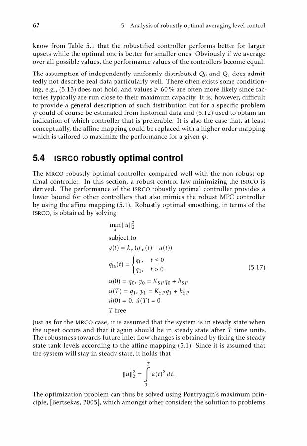
62 5 Analysis of robustly optimal averaging level control
know from Table 5.1 that the robustified controller performs better for largerupsets while the optimal one is better for smaller ones. Obviously if we averageover all possible values, the performance values of the controllers become equal.
The assumption of independently uniformly distributed Q0 and Q1 does admit-tedly not describe real data particularly well. There often exists some condition-ing, e.g., (5.13) does not hold, and values & 60 % are often more likely since fac-tories typically are run close to their maximum capacity. It is, however, difficultto provide a general description of such distribution but for a specific problemϕ could of course be estimated from historical data and (5.12) used to obtain anindication of which controller that is preferable. It is also the case that, at leastconceptually, the affine mapping could be replaced with a higher order mappingwhich is tailored to maximize the performance for a given ϕ.
5.4 ISRCO robustly optimal control
The mrco robustly optimal controller compared well with the non-robust op-timal controller. In this section, a robust control law minimizing the isrco isderived. The performance of the isrco robustly optimal controller provides alower bound for other controllers that also mimics the robust MPC controllerby using the affine mapping (5.1). Robustly optimal smoothing, in terms of theisrco, is obtained by solving
minu||u||22
subject to
y(t) = kv (qin(t) − u(t))
qin(t) =
q0, t ≤ 0q1, t > 0
u(0) = q0, y0 = KSP q0 + bSPu(T ) = q1, y1 = KSP q1 + bSPu(0) = 0, u(T ) = 0
T free
(5.17)
Just as for the mrco case, it is assumed that the system is in steady state whenthe upset occurs and that it again should be in steady state after T time units.The robustness towards future inlet flow changes is obtained by fixing the steadystate tank levels according to the affine mapping (5.1). Since it is assumed thatthe system will stay in steady state, it holds that
||u||22 =
T∫0
u(t)2 dt.
The optimization problem can thus be solved using Pontryagin’s maximum prin-ciple, [Bertsekas, 2005], which amongst other considers the solution to problems
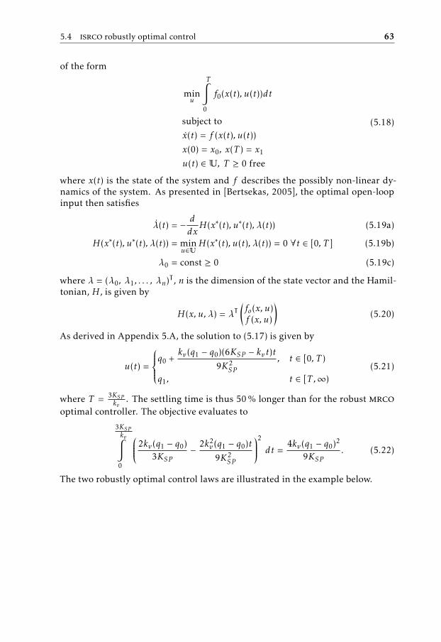
5.4 isrco robustly optimal control 63
of the form
minu
T∫0
f0(x(t), u(t))dt
subject to
x(t) = f (x(t), u(t))
x(0) = x0, x(T ) = x1
u(t) ∈ U, T ≥ 0 free
(5.18)
where x(t) is the state of the system and f describes the possibly non-linear dy-namics of the system. As presented in [Bertsekas, 2005], the optimal open-loopinput then satisfies
λ(t) = − ddxH(x∗(t), u∗(t), λ(t)) (5.19a)
H(x∗(t), u∗(t), λ(t)) = minu∈U
H(x∗(t), u(t), λ(t)) = 0 ∀t ∈ [0, T ] (5.19b)
λ0 = const ≥ 0 (5.19c)
where λ = (λ0, λ1, . . . , λn)T, n is the dimension of the state vector and the Hamil-tonian, H , is given by
H(x, u, λ) = λT(fo(x, u)f (x, u)
)(5.20)
As derived in Appendix 5.A, the solution to (5.17) is given by
u(t) =
q0 +kv(q1 − q0)(6KSP − kv t)t
9K2SP
, t ∈ [0, T )
q1, t ∈ [T ,∞)(5.21)
where T = 3KSPkv
. The settling time is thus 50 % longer than for the robust mrcooptimal controller. The objective evaluates to
3KSPkv∫
0
2kv(q1 − q0)3KSP
−2k2
v (q1 − q0)t
9K2SP
2
dt =4kv(q1 − q0)2
9KSP. (5.22)
The two robustly optimal control laws are illustrated in the example below.
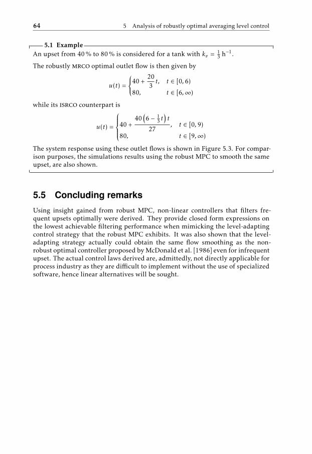
64 5 Analysis of robustly optimal averaging level control
5.1 ExampleAn upset from 40 % to 80 % is considered for a tank with kv = 1
3 h−1.
The robustly mrco optimal outlet flow is then given by
u(t) =
40 +203t, t ∈ [0, 6)
80, t ∈ [6,∞)
while its isrco counterpart is
u(t) =
40 +40
(6 − 1
3 t)t
27, t ∈ [0, 9)
80, t ∈ [9,∞)
The system response using these outlet flows is shown in Figure 5.3. For compar-ison purposes, the simulations results using the robust MPC to smooth the sameupset, are also shown.
5.5 Concluding remarks
Using insight gained from robust MPC, non-linear controllers that filters fre-quent upsets optimally were derived. They provide closed form expressions onthe lowest achievable filtering performance when mimicking the level-adaptingcontrol strategy that the robust MPC exhibits. It was also shown that the level-adapting strategy actually could obtain the same flow smoothing as the non-robust optimal controller proposed by McDonald et al. [1986] even for infrequentupset. The actual control laws derived are, admittedly, not directly applicable forprocess industry as they are difficult to implement without the use of specializedsoftware, hence linear alternatives will be sought.
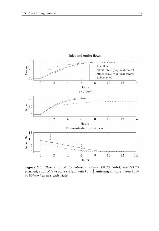
5.5 Concluding remarks 65
0 2 4 6 8 10 12 1440
60
80
Hours
Perc
ent
Tank level
0 2 4 6 8 10 12 1440
60
80
Hours
Perc
ent
Inlet and outlet flows
Inlet flowisrco robustly optimal controlmrco robustly optimal controlRobust MPC
0 2 4 6 8 10 12 140
5
10
15
Hours
Perc
ent/
h
Differentiated outlet flow
Figure 5.3: Illustration of the robustly optimal isrco (solid) and mrco(dashed) control laws for a system with kv = 1
3 suffering an upset from 40 %to 80 % when in steady state.
Appendix
5.A Derivation of the ISRCO optimal control law
First we note that (5.17) is not on the standard form (5.18). This can be obtainedby introducing an artificial input v = u and augmenting the state vector. Thenew state vector is thus x = (y, u)T, where y is the tank level and u is the actualoutlet flow. The dynamics of the system is then given by
x(t) = Ax(t) + Bqinqin(t) + Bvv(t)
where
A =(0 −kv0 0
), Bqin
=(kv0
), Bv =
(01
). (5.23)
Introduce a joint constraint for the initial and end values for the tank level andoutlet into the vectors x0 and x1 as
x0 =(KSP q0 + bSP
q0
), x1 =
(KSP q1 + bSP
q1
). (5.24)
The optimal control problem (5.17) is then equivalent to
minv
T∫0
v(t)2 dt
subject to
x(t) = Ax(t) + Bqinqin(t) + Bvv(t)
qin(t) =
q0, t ≤ 0q1, t > 0
x(0) = x0, x(T ) = x1
v(0) = 0, v(T ) = 0
T free
(5.25)
66
5.A Derivation of the isrco optimal control law 67
When solving the problem the standard case with λ0 > 0, and the pathologicalcase when λ0 = 0 are dealt with separately. In the latter, the cost integral doesnot affect the criterion and since that is the only cost element, one could expectthat the situation λ0 = 0 will not be optimal.
The case λ0 > 0
Without loss of generality, [Bertsekas, 2005], it is assumed that λ = 1. This givesthe Hamiltonian
H(x, v, λ) = v2 + λ1(−kvu + kvqin) + λ2v. (5.26)
The adjoint equation (5.19a) gives thatλ1 = 0λ2 = −kvλ1
⇒
λ1 = c1
λ2 = −kvc1t + c2(5.27)
for some constants c1 and c2. Inserting this into (5.26) and minimizing the Hamil-tonian
minv
v(0)=v(T )=0
v2 + c1kv(−u + qin) + (c2 − kvc1t)v
= minv
v(0)=v(T )=0
(v − kvc1t − c2
2
)2
−(kvc1t − c2
2
)2
+ c1kv(−u + qin),(5.28)
yields the optimal artificial input
v(t) =
0, t ≤ 0c1kv t − c2
2, 0 < t < T
0, t ≥ T
(5.29)
Using that H(x∗, v∗, λ) = 0 for all t ∈ [0, T ], we evaluate it for t = T
H(x∗(T ), v∗(T ), λ) = −(kvc1T − c2
2
)2
+ c1kv(−q1 + q1) = 0⇔ c2 = kvc1T . (5.30)
The value of the state vector at t = T then evaluates to
u(T ) = q0 +c1kvT
2 − 2c1kvT2
4= q0 −
c1kvT2
4(5.31a)
y(T ) = KSP q0 + bSP + kvT (q1 − q0) +k2v c1T
3
6(5.31b)
Using the end-value constraint x(T ) = x1 gives
− c1kvT2
4= q1 − q0 (5.32a)
kvT (q1 − q0) +k2v c1T
3
6= KSP (q1 − q0) (5.32b)
68 5 Analysis of robustly optimal averaging level control
Rewriting (5.32b) gives that T evaluates to
kvT (q1 − q0) − 2T kv3
(−kvc1T
2
4
)︸ ︷︷ ︸
=q1−q0
= KSP (q1 − q0)⇔
kvT3
(q1 − q0) = KSP (q1 − q0)⇔ T =3KSPkv
.
(5.33)
The constant c1 can then be found by inserting this into (5.32a)
−9K2
SP c1
4kv= q1 − q0⇔ c1 =
−4kv(q1 − q0)
9K2SP
. (5.34)
The optimal outlet flow when λ0 > 0 is thus given by
u(t) = q0 +c1kv t
2 − 2c2t4
= q0 +kv(q1 − q0)(6KSP − kv t)t
9K2SP
. (5.35)
Ultimately, the objective evaluates to
3KSPkv∫
0
2kv(q1 − q0)3KSP
−2k2
v (q1 − q0)t
9K2SP
2
dt =4kv(q1 − q0)2
9KSP. (5.36)
The case λ0 = 0
λ0 = 0 in (5.26) along with the expression for λ1 and λ2 from (5.27) give theHamiltonian
H = c1kv(−u + qin) + (c2 − kvc1t)v. (5.37)
The optimal input is thus given by
v(t) =
0, t ≤ 0c0, 0 < t ≤ t′
c′ , t′ < t < T
0, t ≥ T
(5.38)
where c0 and c′ are constants of opposite sign and t′ is the time when c2 − kvc1tchanges sign, i.e., c2 − kvc1t
′ = 0. Since H(x∗, v∗, λ) = 0∀t ∈ [0, T ] it must holdfor t = t′ , from which it follows that
H = c1kv(−u∗(t′) + q1) + (c2 − c1kv t′)︸ ︷︷ ︸
=0
c0 = 0⇔
u∗(t′) = q1.
(5.39)
So, the outlet flow will have obtained its end-value, q1, at the time t′ and we shallnow see what implications this have. Let us consider the case q1 > q0 (q1 < q0follows analogously), it then follows that c0 > 0 and c′ < 0 since u > 0 is needed
5.A Derivation of the isrco optimal control law 69
initially to obtain u(t′) = q1. If then c′ is deployed for t ∈ (t′ , T ], u will decrease.But since u(t′) = q1 already, the only possibility that the constraint u(T ) = q1 willbe fulfilled is if t′ = T (or equivalently c′ = 0). Consequently, the optimal inputis
v(t) =
0, t ≤ 0c0, 0 < t < T0, t ≥ T
(5.40)
Recognizing this expression as the derivative of the mrco optimal control lawfrom Sections 2.3 and 5.2, it follows that
c0 =kv(q1 − q0)
2KSP, T =
2KSPkv
.
The outlet flow is then given by
u(t) = q0 +kv(q1 − q0)
2KSPt
and the performance criterion evaluates to
kv(q1 − q0)2
2KSPwhich obviously is larger than (5.36). Hence, the open loop control law (5.35) isthe optimal solution to (5.17).

6Linear control of surge tanks
suffering from frequent flow upsets
In the previous chapter we investigated the idea to mimic the robust MPC con-troller by enforcing other controllers and control structures to position theirsteady state tank level according to an affine mapping. In this chapter, two linearcontrollers that mimic the robust MPC are presented and analyzed. They canbe rather straightforwardly implemented in an industrial control system. Com-pared to the optimal non-linear controllers and the robust MPC, these linear con-trollers thus have larger applicability for the process industry. The drawbackis that some filtering performance is lost compared to the robustly optimal con-trollers presented in Chapter 5. Most parts of this chapter have previously beenpublished in [Rosander et al., 2012b].
The obvious linear controller that displays the same level-adaption as the robustMPC, is the P controller. The properties of this controller and some implementa-tion aspects are discussed in Section 6.1. In Section 6.2 a novel control structureis proposed with a PI controller that also adapts the steady state tank level. InSection 6.3 the optimal tuning of this PI controller is derived. With this tun-ing, the noise sensitivity of the P and the proposed PI controller are analyzed inSection 6.4. The proposed controllers are compared to a standard PI controllerand the result is presented in Section 6.5 before the chapter is concluded in Sec-tion 6.6.
6.1 P controller
The P controller is the obvious choice of a linear controller that displays the samebehavior as the robust MPC controller, as has been discussed in the precedingchapters. Here the performance and some implementation aspects will be stud-
71
72 6 Linear control of surge tanks suffering from frequent flow upsets
ied. To simplify the readability, a condensed presentation of the controller willbe given.
As presented in Section 2.5, a P controller is given by
u(t) = Kp(r − y(t)) + bp = −Kpy(t) + Kpr + bp︸ ︷︷ ︸bp
, (6.1)
and to mimic the robust MPC, the parameters should be chosen according to
Kp = −qmax − qmin
ymax − ymin,
bp =qminymax − qmaxymin
ymax − ymin.
(6.2)
For an inlet flow step change from q0 to q1 when in steady state, the mrco andisrco performance values of the P controller evaluate to
||u||22 = −(q1 − q0)2kvKp
2,
||u||∞ = −|q1 − q0|kvKp,(6.3)
where the minus signs come from the fact that Kp < 0 is needed to obtain stability.Given this information, the P controller will now be further analyzed.
6.1.1 Performance evaluation
In Chapter 2 it was shown that the P controller gives quite poor flow smoothingin terms of the mrco. In that chapter, the comparison was made with “non-robust” controllers. Comparing its performance, (6.3), with the robustly optimalcontrollers from Chapter 5 provides an evaluation on how well the P controllermatches against the robustly optimal. By noting that KSP = − 1
Kpfor the affine
mapping (5.1-5.2) and using the performance expressions for the robustly opti-mal controllers, (5.11) and (5.22), we can conclude that in terms of the isrcothe performance of the P controller is only 12 % worse, while the mrco actuallyis twice as bad. In terms of the isrco, the P controller thus compares very wellwith the optimal controllers. The difference inmrcowould preferably have beenless. Still, the P controller is a much simpler control structure than the optimalcontroller, so there should not come as a surprise that some performance mightbe lost.
6.1.2 Implementation aspects
The P controller is conceptually easy to implement, just specify the limits on qinand y and use (6.2) to obtain Kp and bp. Implementing these in a DCS is, however,a bit more tricky. First of all the “true” bias parameter bp is typically not avail-able since it is used to obtain bump less transfer between manual and automatic
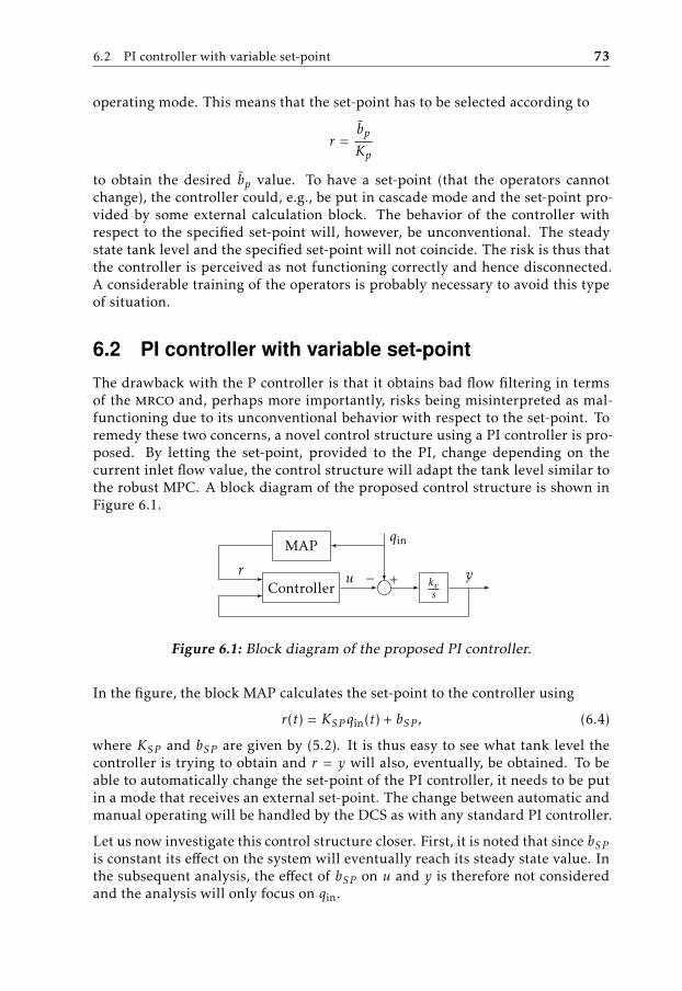
6.2 PI controller with variable set-point 73
operating mode. This means that the set-point has to be selected according to
r =bpKp
to obtain the desired bp value. To have a set-point (that the operators cannotchange), the controller could, e.g., be put in cascade mode and the set-point pro-vided by some external calculation block. The behavior of the controller withrespect to the specified set-point will, however, be unconventional. The steadystate tank level and the specified set-point will not coincide. The risk is thus thatthe controller is perceived as not functioning correctly and hence disconnected.A considerable training of the operators is probably necessary to avoid this typeof situation.
6.2 PI controller with variable set-point
The drawback with the P controller is that it obtains bad flow filtering in termsof the mrco and, perhaps more importantly, risks being misinterpreted as mal-functioning due to its unconventional behavior with respect to the set-point. Toremedy these two concerns, a novel control structure using a PI controller is pro-posed. By letting the set-point, provided to the PI, change depending on thecurrent inlet flow value, the control structure will adapt the tank level similar tothe robust MPC. A block diagram of the proposed control structure is shown inFigure 6.1.
Controller
MAP
kvs
r
qin
+u − y
Figure 6.1: Block diagram of the proposed PI controller.
In the figure, the block MAP calculates the set-point to the controller using
r(t) = KSP qin(t) + bSP , (6.4)
where KSP and bSP are given by (5.2). It is thus easy to see what tank level thecontroller is trying to obtain and r = y will also, eventually, be obtained. To beable to automatically change the set-point of the PI controller, it needs to be putin a mode that receives an external set-point. The change between automatic andmanual operating will be handled by the DCS as with any standard PI controller.
Let us now investigate this control structure closer. First, it is noted that since bSPis constant its effect on the system will eventually reach its steady state value. Inthe subsequent analysis, the effect of bSP on u and y is therefore not consideredand the analysis will only focus on qin.
74 6 Linear control of surge tanks suffering from frequent flow upsets
6.2.1 Transfer functions
The block Controller in the block diagram in Figure 6.1 is a standard PI controllerwith a β-factor on the set-point
U (s) = Kc
(βR(s) − Y (s) +
1TI s
(R(s) − Y (s))). (6.5)
Using R(s) = KSPQin(s) + bSPs (and neglecting the effect bSP has), the resulting
closed loop dynamics become
Y (s) =kv (TI s − KcβKSP TI s − KcKSP )
TI s2 − kvKcTI s − kvKcQin(s),
U (s) =Kc
(βKSP TI s
2 + (KSP − kvTI )s − kv)
TI s2 − kvKcTI s − kvKcQin(s).
(6.6)
6.3 Tuning of the PI controller
When adapting the set-point of the PI controller, the steady state tank level willbe the same as for the P controller (as well as for the robustly optimal controllers).The PI controller is, however, dynamic and thus there is a risk that it will have astep response with, for example an overshoot. Such behavior can not be tolerated,since that could result in violation of the level constraint if the flow is close toqmin or qmax. It is thus required that the PI controller is tuned so that the transferfunctions (6.6) give rise to a step response without over- or undershoots1.
Before turning to investigate the under- and overshoots of the system, it is firstnoted that the controller has a direct term from the inlet to the outlet flow
βKcKSP .
A step in the inlet flow will thus give a discontinuous outlet flow which obviouslycontradicts the main idea of using surge tanks. It is also the case that neither theisrco nor the mrco as defined by (2.3) and (2.5) exist for discontinuous outletflows. The obvious choice is thus β = 0 which will decouple the outlet from theinlet flow. This modification yields the closed loop transfer functions
Y (s) =kv (TI s − KcKSP )
TI s2 − kvKcTI s − kvKcQin(s), (6.7a)
U (s) =Kc ((KSP − kvTI ) s − kv)TI s2 − kvKcTI s − kvKc
Qin(s). (6.7b)
Both systems are thus of the form
Ks + z
(s + p1)(s + p2)
1Strictly speaking this is only required close to the boundary and might thus be obtained with anon-linear gain.
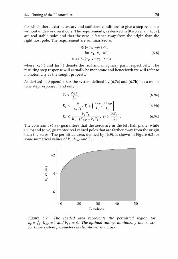
6.3 Tuning of the PI controller 75
for which there exist necessary and sufficient conditions to give a step responsewithout under- or overshoots. The requirements, as derived in [Kwon et al., 2002],are real stable poles and that the zero is farther away from the origin than therightmost pole. The requirement are summarized as
<−p1, −p2 <0,
=p1, p2 =0,
max<−p1, −p2 ≥ − z(6.8)
where < · and = · denote the real and imaginary part, respectively. Theresulting step response will actually be monotone and henceforth we will refer tomonotonicity as the sought property.
As derived in Appendix 6.A the system defined by (6.7a) and (6.7b) has a mono-tone step response if and only if
TI >KSPkv
, (6.9a)
Kc ≤ −4kvTI
, TI ∈(KSPkv
,2KSPkv
], (6.9b)
Kc ≤kvTI
KSP (KSP − kvTI ), TI >
2KSPkv
. (6.9c)
The constraint (6.9a) guarantees that the zeros are in the left half plane, while(6.9b) and (6.9c) guarantee real valued poles that are farther away from the originthan the zeros. The permitted area, defined by (6.9), is shown in Figure 6.2 forsome numerical values of kv , KSP and bSP .
10 20 30 40 50
−6
−4
−2
TI values
Kc
valu
es
Figure 6.2: The shaded area represents the permitted region forkv = 1
10 , KSP = 1 and bSP = 0. The optimal tuning, minimizing the isrco,for these system parameters is also shown as a cross.
76 6 Linear control of surge tanks suffering from frequent flow upsets
6.3.1 Optimal performance for a step upset
Provided that the parameters fulfill (6.9) how should they be chosen to achieveoptimal filtering? If the isrco is minimized, the optimal tuning can be derivedanalytically. Under the assumption of a step disturbance2 of size (q1 − q0), wethus want to find the solution to
minKc , TI
J = ||u||22
subject to
U (s) =Kc ((KSP − kvTI ) s − kv)TI s2 − kvKcTI s − kvKc
q1 − q0
s
TI >KSPkv
Kc ≤ −4kvTI
, TI ∈(KSPkv
,2KSPkv
]Kc ≤
kvTIKSP (KSP − kvTI )
, TI >2KSPkv
(6.10)
The optimal value will either be obtained on the boundary or at a stationary point.By investigating these possibilities, an analytical expression for the optimal val-ues on Kc and TI can be derived.
Kc and TI not on the boundary
For Kc and TI not on the boundary, the system is an over damped second ordersystem whose time response is
u(t) = K
((z − p1)e−p1t − (z − p2)e−p2t
p2 − p1
)where K = Kc(q1−q0)(KSP −kvTI )
TIand −p1, −p2 and −z are the poles and zero of (6.7b),
see (6.22) and (6.23). Squaring and integrating the obtained expression gives theperformance value
J =(2kvTIKSP − K2
SP − k2vT
2I )Kc + kvTI
2kvT2I
(q1 − q0)2. (6.11)
Investigating this expression closer, we note that
∂J∂Kc
=(2kvTIKSP − K2SP − k
2vT
2I )(q1 − q0)2 =
− (kvTI − KSP )2 (q1 − q0)2 < 0.(6.12)
The objective function thus decreases with an increasing Kc. Hence, it will beoptimal to choose Kc on the boundary.
2Note that, in contrast to, a standard PI controller (e.g. the ones described in Section 2.3.1), thesize of the step does not have any effect on what upset sizes the controller can handle (c.f. Amax in(2.13) and (2.14)). It is already built into the structure that the system will stay within bounds for allupsets between qmin and qmax.
6.3 Tuning of the PI controller 77
Kc on the boundary
With Kc on the boundary, there exist two possibilities as either (6.9b) or (6.9c)will hold with equality. For
Kc =kvTI
KSP (KSP − kvTI ),
pole zero cancellation occurs (regardless of TI value) and the PI controller obtainsthe same isrco as the P controller
kv2KSP
(q1 − q0)2. (6.13)
For Kc = − 4kvTI
, the system has a double pole and obtains
J =5k2
vT2I + 4K2
SP − 8kvTIKSP2k2
vT3I
(q1 − q0)2. (6.14)
The optimal TI -value for (6.14) can be derived by solving
d JdTI
=0,d2 J
dT 2I
> 0⇔
5k2vT
2I − 16kvTIKSP + 12K2
SP
−2k2vT
4I
=0,5k2
vT2I − 24kvTIKSP + 24K2
SP
k2vT
5I
> 0
yielding
TI =6KSP5kv
. (6.15)
Inserting this into (6.14) gives the optimal objective function value
J(K∗c , T∗I ) =
25kv54KSP
(q1 − q0)2. (6.16)
Concluding, the tuning which minimizes the isrco for an inlet flow step distur-bance is
Kc = − 4kvTI
,
TI =6KSP5kv
.(6.17)
Inserting the optimal TI value into the expressions for Kc, gives that Kc = −103KSP
.The gain is thus constant regardless of the size of the tank. With this tuning, themrco of the controller evaluates to
||u||∞ =10|q1 − q0|kve−
12
9KSP. (6.18)
Let us compare the performance for the proposed PI controller with that of the
78 6 Linear control of surge tanks suffering from frequent flow upsets
Table 6.1: The performance values for an inlet flow step change for the pro-posed PI controller, the P controller and the robustly optimal controllers.
Controller mrco isrco
PI 10e−0.5kv9KSP
25kv54KSP
P kvKSP
kv2KSP
Robustly optimal kv2KSP
4kv9KSP
robustly optimal controllers and the P controller. In Table 6.1, the performanceexpressions for both the linear and non-linear controllers are summarized. Forthe isrco, the PI controller performs 4 % worse than the optimal controller but7 % better than the P controller. In terms of the isrco, there is thus not muchdifference between the linear controllers and the optimal non-linear controller.For the mrco, the difference in performance between the controllers is larger, asthe optimal controller outperforms the PI with 35 % which in turn is 33 % betterthan the P controller. If instead parameters minimizing the mrco are used3, themrco of the PI could have been improved with approximately 5 %.
The tuning (6.17) and the resulting outlet flow and tank level for the proposed PIcontroller is illustrated in the example below.
6.1 ExampleThe same setup as the examples in Chapter 2 is considered, i.e., an upset from40 % to 80 % for a tank with kv = 1
3 and KSP = 1. The system parameters give thetuning
Kc = −3.33 and TI = 3.6 h.
The result of this tuning is shown in Figure 6.3. For comparison purposes, alsothe outlet flow and tank level of the P controller is shown. As can be seen in thefigure, there is not much of a difference in the qualitative behavior of the twocontrollers. The performance of the PI controller for this upset evaluates to
||u||∞ = 9.0
||u||22 = 247
whereas the P controller obtains
||u||∞ = 13.3
||u||22 = 267
3When minimizing the mrco, there do however not exist any closed form expressions.
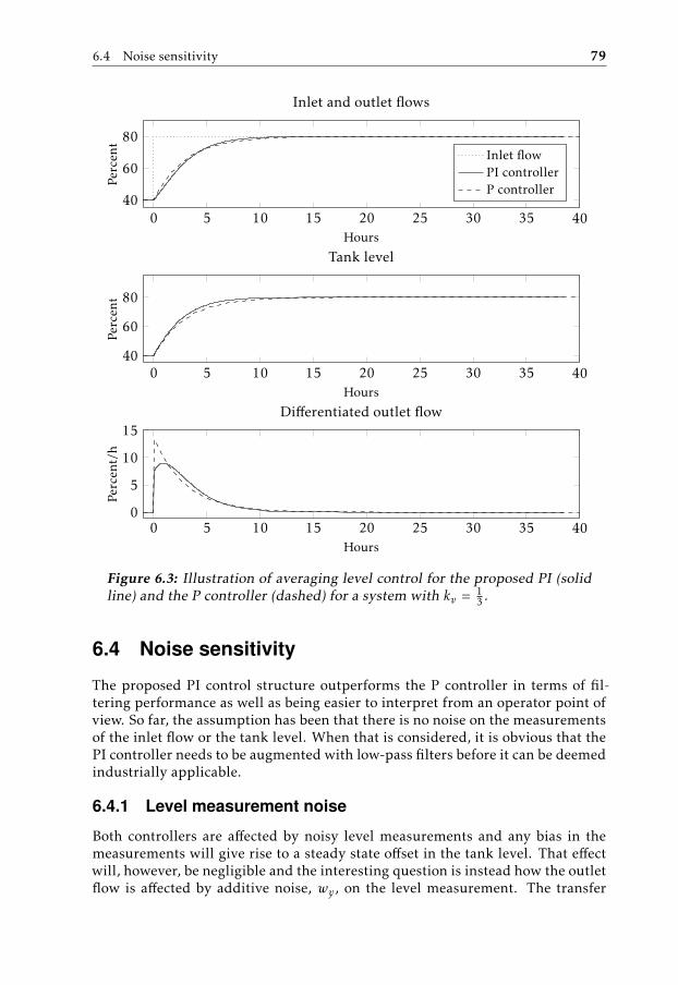
6.4 Noise sensitivity 79
0 5 10 15 20 25 30 35 4040
60
80
Hours
Perc
ent
Tank level
0 5 10 15 20 25 30 35 4040
60
80
Hours
Perc
ent
Inlet and outlet flows
Inlet flowPI controllerP controller
0 5 10 15 20 25 30 35 400
5
10
15
Hours
Perc
ent/
h
Differentiated outlet flow
Figure 6.3: Illustration of averaging level control for the proposed PI (solidline) and the P controller (dashed) for a system with kv = 1
3 .
6.4 Noise sensitivity
The proposed PI control structure outperforms the P controller in terms of fil-tering performance as well as being easier to interpret from an operator point ofview. So far, the assumption has been that there is no noise on the measurementsof the inlet flow or the tank level. When that is considered, it is obvious that thePI controller needs to be augmented with low-pass filters before it can be deemedindustrially applicable.
6.4.1 Level measurement noise
Both controllers are affected by noisy level measurements and any bias in themeasurements will give rise to a steady state offset in the tank level. That effectwill, however, be negligible and the interesting question is instead how the outletflow is affected by additive noise, wy , on the level measurement. The transfer
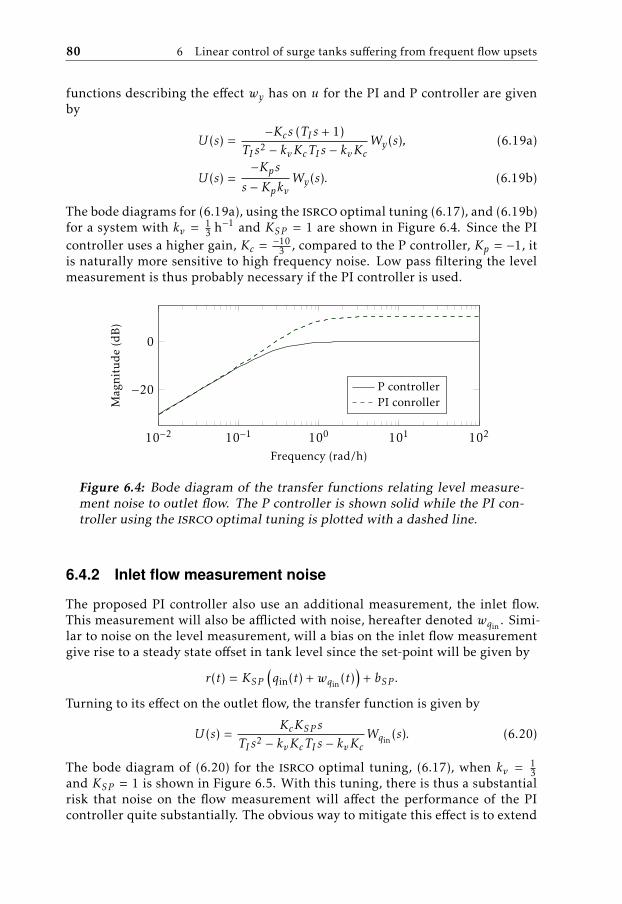
80 6 Linear control of surge tanks suffering from frequent flow upsets
functions describing the effect wy has on u for the PI and P controller are givenby
U (s) =−Kcs (TI s + 1)
TI s2 − kvKcTI s − kvKcWy(s), (6.19a)
U (s) =−Kps
s − KpkvWy(s). (6.19b)
The bode diagrams for (6.19a), using the isrco optimal tuning (6.17), and (6.19b)for a system with kv = 1
3 h−1 and KSP = 1 are shown in Figure 6.4. Since the PIcontroller uses a higher gain, Kc = −10
3 , compared to the P controller, Kp = −1, itis naturally more sensitive to high frequency noise. Low pass filtering the levelmeasurement is thus probably necessary if the PI controller is used.
10−2 10−1 100 101 102
−20
0
Frequency (rad/h)
Mag
nitu
de
(dB
)
P controllerPI conroller
Figure 6.4: Bode diagram of the transfer functions relating level measure-ment noise to outlet flow. The P controller is shown solid while the PI con-troller using the isrco optimal tuning is plotted with a dashed line.
6.4.2 Inlet flow measurement noise
The proposed PI controller also use an additional measurement, the inlet flow.This measurement will also be afflicted with noise, hereafter denoted wqin
. Simi-lar to noise on the level measurement, will a bias on the inlet flow measurementgive rise to a steady state offset in tank level since the set-point will be given by
r(t) = KSP(qin(t) + wqin
(t))
+ bSP .
Turning to its effect on the outlet flow, the transfer function is given by
U (s) =KcKSP s
TI s2 − kvKcTI s − kvKcWqin
(s). (6.20)
The bode diagram of (6.20) for the isrco optimal tuning, (6.17), when kv = 13
and KSP = 1 is shown in Figure 6.5. With this tuning, there is thus a substantialrisk that noise on the flow measurement will affect the performance of the PIcontroller quite substantially. The obvious way to mitigate this effect is to extend
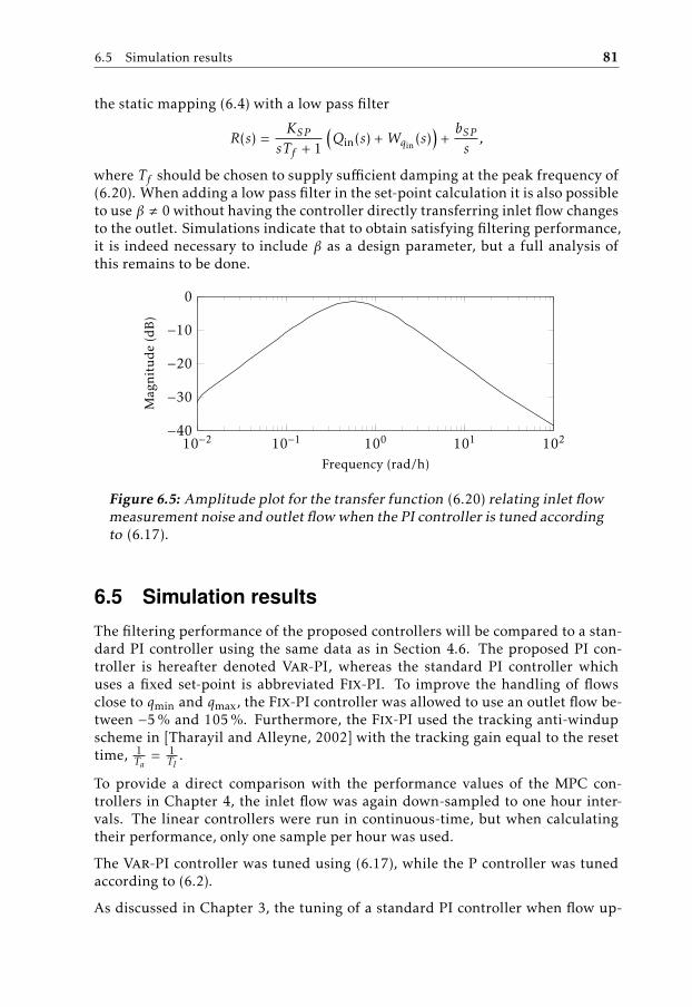
6.5 Simulation results 81
the static mapping (6.4) with a low pass filter
R(s) =KSP
sTf + 1
(Qin(s) + Wqin
(s))
+bSPs,
where Tf should be chosen to supply sufficient damping at the peak frequency of(6.20). When adding a low pass filter in the set-point calculation it is also possibleto use β , 0 without having the controller directly transferring inlet flow changesto the outlet. Simulations indicate that to obtain satisfying filtering performance,it is indeed necessary to include β as a design parameter, but a full analysis ofthis remains to be done.
10−2 10−1 100 101 102−40
−30
−20
−10
0
Frequency (rad/h)
Mag
nitu
de
(dB
)
Figure 6.5: Amplitude plot for the transfer function (6.20) relating inlet flowmeasurement noise and outlet flow when the PI controller is tuned accordingto (6.17).
6.5 Simulation results
The filtering performance of the proposed controllers will be compared to a stan-dard PI controller using the same data as in Section 4.6. The proposed PI con-troller is hereafter denoted Var-PI, whereas the standard PI controller whichuses a fixed set-point is abbreviated Fix-PI. To improve the handling of flowsclose to qmin and qmax, the Fix-PI controller was allowed to use an outlet flow be-tween −5 % and 105 %. Furthermore, the Fix-PI used the tracking anti-windupscheme in [Tharayil and Alleyne, 2002] with the tracking gain equal to the resettime, 1
Ta= 1
TI.
To provide a direct comparison with the performance values of the MPC con-trollers in Chapter 4, the inlet flow was again down-sampled to one hour inter-vals. The linear controllers were run in continuous-time, but when calculatingtheir performance, only one sample per hour was used.
The Var-PI controller was tuned using (6.17), while the P controller was tunedaccording to (6.2).
As discussed in Chapter 3, the tuning of a standard PI controller when flow up-
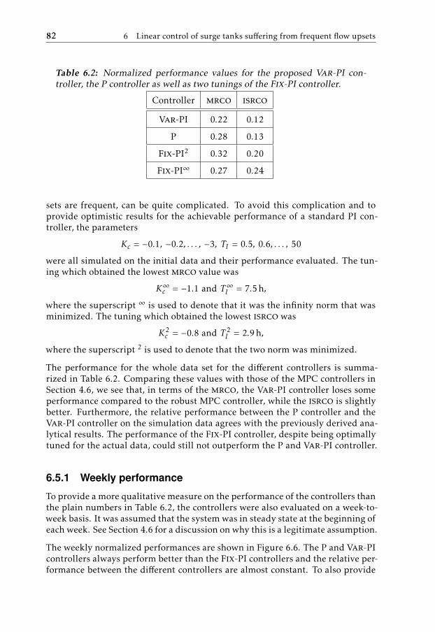
82 6 Linear control of surge tanks suffering from frequent flow upsets
Table 6.2: Normalized performance values for the proposed Var-PI con-troller, the P controller as well as two tunings of the Fix-PI controller.
Controller mrco isrco
Var-PI 0.22 0.12
P 0.28 0.13
Fix-PI2 0.32 0.20
Fix-PI∞ 0.27 0.24
sets are frequent, can be quite complicated. To avoid this complication and toprovide optimistic results for the achievable performance of a standard PI con-troller, the parameters
Kc = −0.1, −0.2, . . . , −3, TI = 0.5, 0.6, . . . , 50
were all simulated on the initial data and their performance evaluated. The tun-ing which obtained the lowest mrco value was
K∞c = −1.1 and T∞I = 7.5 h,
where the superscript ∞ is used to denote that it was the infinity norm that wasminimized. The tuning which obtained the lowest isrco was
K2c = −0.8 and T 2
I = 2.9 h,
where the superscript 2 is used to denote that the two norm was minimized.
The performance for the whole data set for the different controllers is summa-rized in Table 6.2. Comparing these values with those of the MPC controllers inSection 4.6, we see that, in terms of the mrco, the Var-PI controller loses someperformance compared to the robust MPC controller, while the isrco is slightlybetter. Furthermore, the relative performance between the P controller and theVar-PI controller on the simulation data agrees with the previously derived ana-lytical results. The performance of the Fix-PI controller, despite being optimallytuned for the actual data, could still not outperform the P and Var-PI controller.
6.5.1 Weekly performance
To provide a more qualitative measure on the performance of the controllers thanthe plain numbers in Table 6.2, the controllers were also evaluated on a week-to-week basis. It was assumed that the system was in steady state at the beginning ofeach week. See Section 4.6 for a discussion on why this is a legitimate assumption.
The weekly normalized performances are shown in Figure 6.6. The P and Var-PIcontrollers always perform better than the Fix-PI controllers and the relative per-formance between the different controllers are almost constant. To also provide
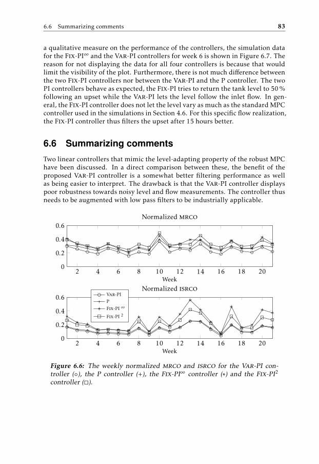
6.6 Summarizing comments 83
a qualitative measure on the performance of the controllers, the simulation datafor the Fix-PI∞ and the Var-PI controllers for week 6 is shown in Figure 6.7. Thereason for not displaying the data for all four controllers is because that wouldlimit the visibility of the plot. Furthermore, there is not much difference betweenthe two Fix-PI controllers nor between the Var-PI and the P controller. The twoPI controllers behave as expected, the Fix-PI tries to return the tank level to 50 %following an upset while the Var-PI lets the level follow the inlet flow. In gen-eral, the Fix-PI controller does not let the level vary as much as the standard MPCcontroller used in the simulations in Section 4.6. For this specific flow realization,the Fix-PI controller thus filters the upset after 15 hours better.
6.6 Summarizing comments
Two linear controllers that mimic the level-adapting property of the robust MPChave been discussed. In a direct comparison between these, the benefit of theproposed Var-PI controller is a somewhat better filtering performance as wellas being easier to interpret. The drawback is that the Var-PI controller displayspoor robustness towards noisy level and flow measurements. The controller thusneeds to be augmented with low pass filters to be industrially applicable.
2 4 6 8 10 12 14 16 18 200
0.2
0.4
0.6
Week
Normalized mrco
2 4 6 8 10 12 14 16 18 200
0.2
0.4
0.6
Week
Normalized isrcoVar-PI
P
Fix-PI ∞
Fix-PI 2
Figure 6.6: The weekly normalized mrco and isrco for the Var-PI con-troller (), the P controller (+), the Fix-PI∞ controller (∗) and the Fix-PI2
controller ().
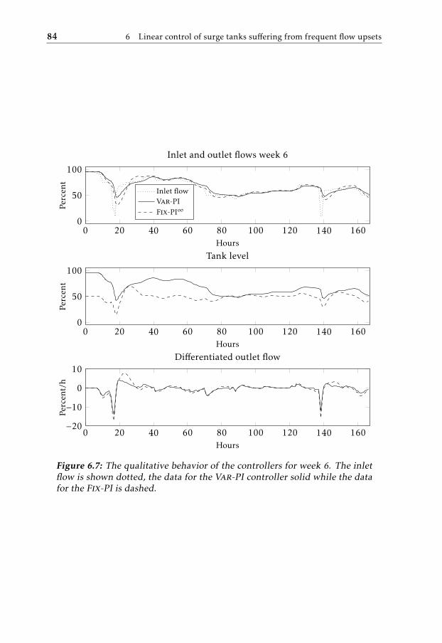
84 6 Linear control of surge tanks suffering from frequent flow upsets
0 20 40 60 80 100 120 140 1600
50
100
Hours
Perc
ent
Tank level
0 20 40 60 80 100 120 140 1600
50
100
Hours
Perc
ent
Inlet and outlet flows week 6
Inlet flowVar-PI
Fix-PI∞
0 20 40 60 80 100 120 140 160−20
−10
0
10
Hours
Perc
ent/
h
Differentiated outlet flow
Figure 6.7: The qualitative behavior of the controllers for week 6. The inletflow is shown dotted, the data for the Var-PI controller solid while the datafor the Fix-PI is dashed.
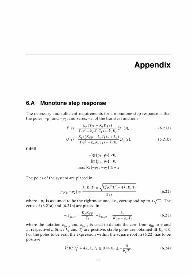
Appendix
6.A Monotone step response
The necessary and sufficient requirements for a monotone step response is thatthe poles, −p1 and −p2, and zeros, −z, of the transfer functions
Y (s) =kv (TI s − KcKSP )
TI s2 − kvKcTI s − kvKcQin(s), (6.21a)
U (s) =Kc ((KSP − kvTI ) s + kv)TI s2 − kvKcTI s − kvKc
Qin(s). (6.21b)
fulfill
−<p1, p2 <0,
=p1, p2 =0,
max<−p1, −p2 ≥ − z
The poles of the system are placed in
−p1,−p2 =kvKcTI ±
√k2vK
2c T
2I + 4kvKcTI
2TI, (6.22)
where −p1 is assumed to be the rightmost one, i.e., corresponding to +√. . .. Thezeros of (6.21a) and (6.21b) are placed in
− zqin,y =KcKSPTI
, −zqin,u =kv
KSP − kvTI, (6.23)
where the notation zqin,y and zqin,u is used to denote the zero from qin to y andu, respectively. Since kv and TI are positive, stable poles are obtained iff Kc < 0.For the poles to be real, the expression within the square root in (6.22) has to bepositive
k2vK
2c T
2I + 4kvKcTI ≥ 0⇔Kc ≤ −
4kvTI
. (6.24)
85
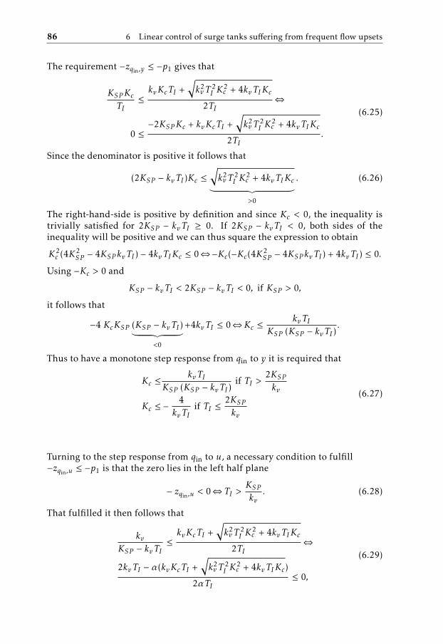
86 6 Linear control of surge tanks suffering from frequent flow upsets
The requirement −zqin,y ≤ −p1 gives that
KSPKcTI
≤kvKcTI +
√k2vT
2I K
2c + 4kvTIKc
2TI⇔
0 ≤−2KSPKc + kvKcTI +
√k2vT
2I K
2c + 4kvTIKc
2TI.
(6.25)
Since the denominator is positive it follows that
(2KSP − kvTI )Kc ≤√k2vT
2I K
2c + 4kvTIKc︸ ︷︷ ︸>0
. (6.26)
The right-hand-side is positive by definition and since Kc < 0, the inequality istrivially satisfied for 2KSP − kvTI ≥ 0. If 2KSP − kvTI < 0, both sides of theinequality will be positive and we can thus square the expression to obtain
K2c (4K2
SP − 4KSP kvTI ) − 4kvTIKc ≤ 0⇔−Kc(−Kc(4K2SP − 4KSP kvTI ) + 4kvTI ) ≤ 0.
Using −Kc > 0 and
KSP − kvTI < 2KSP − kvTI < 0, if KSP > 0,
it follows that
−4 KcKSP (KSP − kvTI )︸ ︷︷ ︸<0
+4kvTI ≤ 0⇔Kc ≤kvTI
KSP (KSP − kvTI ).
Thus to have a monotone step response from qin to y it is required that
Kc ≤kvTI
KSP (KSP − kvTI )if TI >
2KSPkv
Kc ≤ −4kvTI
if TI ≤2KSPkv
(6.27)
Turning to the step response from qin to u, a necessary condition to fulfill−zqin,u ≤ −p1 is that the zero lies in the left half plane
− zqin,u < 0⇔ TI >KSPkv
. (6.28)
That fulfilled it then follows that
kvKSP − kvTI
≤kvKcTI +
√k2vT
2I K
2c + 4kvTIKc
2TI⇔
2kvTI − α(kvKcTI +√k2vT
2I K
2c + 4kvTIKc)
2αTI≤ 0,
(6.29)
6.A Monotone step response 87
where α , KSP − kvTI . Since α < 0 it follows that
−α√k2vT
2I K
2c + 4kvTIKc︸ ︷︷ ︸≥0
≥ kvTI (αKc − 2). (6.30)
For a negative right-hand side
Kc ≥2
KSP − kvTI(6.31)
the inequality is trivially fulfilled and if not both sides can be squared to obtainthe requirement
Kc ≤kvTI
KSP (KSP − kvTI ). (6.32)
So, the requirement is that either (or both) of (6.31) and (6.32) plus the constraint(6.28) hold, for the step response from qin to u to be monotone. Since
−4kvTI
≤ kvTIKSP (KSP − kvTI )
⇔(kvTI − 2KSP )2 ≥ 0, (6.33)
the constraints on Kc imposed by (6.27) are thus more restrictive than (6.31) and(6.32). Consequently, the latter two do not impose any additional restrictions onKc. Combining (6.27) and (6.28) concludes the derivation.

7Industrial case study - revisited
The previous chapters have dealt with the control of a single buffer tank sub-jected to a frequently changing inlet flow. In a sense, these chapters answer thequestion how to control the first tank of the process segment presented in Chap-ter 3, provided that Tank 1 is the only buffer tank available. In this chapter, theflow smoothing when several tanks are available is briefly addressed. The in-sight from Chapter 4, that it is beneficial to adapt the steady state tank level isassumed to hold also in this case, although without any robust MPC simulationsthat reinforces the assumption.
Tuning averaging level controllers in sequence is tricky. For standard PI con-trollers, there is a risk that flow variations are amplified instead of smoothedwhen multiple tanks are used, see Cheung and Luyben [1979a]. That situationcan, however, be avoided by ensuring that the individual closed loop systems donot have their peak response at the same frequency.
This chapter will not provide definite answers, but rather highlight some unan-swered questions when multiple tanks are used for flow smoothing. Implementa-tion aspects as noise sensitivity and other issues will not be considered, the focusis instead on the overall control and tuning strategy that should be used.
7.1 Model of the process segment
For the simulations performed in this chapter a simplified model of the processsegment shown in Figure 3.1 will be used. To separate the different parts of thesegment, an additional subscript is added to all parameters. For example, Kc,1is the gain of the (PI) controller for Tank 1 while kv,3 is the inverse of the fillingtime for Tank 3.
89
90 7 Industrial case study - revisited
The columns will be modeled as constant gains, Ki , i = 1, 2, 3. This is a simpli-fication since they are, of course, dynamic processes. The columns are, however,tightly controlled, making the used model fairly valid. The time constant of thereactor is also short compared to the hold-up time of the tanks. The reactor isthus disregarded and the reactor feed is assumed to be the inlet flow to Tank 1.
The minimum and maximum capacity of the outlet flows from the tanks are as-sumed to equal that of the inlet flow, i.e., (2.2b) is assumed to hold for the indi-vidual tanks. For the actual application, the outlet flows actually have a largercapacity than the inlet flows, but that is not considered. The lower flow limit,qmin, is assumed to be 0 % for all process flows. This is not the lower flow limitfor the actual application since it is costly to stop the columns. For flows belowa certain limit, the columns are thus kept running by recirculating the product.The assumption of equal flow capacity of the different tanks gives that
qmin,1 = qmin,2 = qmin,3 = 0,
qmax,1 = 100,
qmax,2 = 100 ·K1,
qmax,3 = 100 ·K1 ·K2.
The size of the buffer tanks and the assumed flow capacities give that the kv forthe different tanks are
kv,1 =3
10,
kv,2 =4K1
3,
kv,3 =12K1K2
25.
The minimum and maximum tank level of the tanks are set to 20 % and 80 %,respectively. The parameters describing the affine mapping, see (5.1) and (5.2),are thus given by
KSP ,1 = 0.6, bSP ,1 = 20,
KSP ,2 = 1.03, bSP ,2 = 20,
KSP ,2 = 0.95, bSP ,3 = 20.
7.2 Simulation of P and VAR-PI control
The previous chapters showed that to average a frequently changing inlet flow, itis necessary to adapt the steady state tank level. Two linear controllers, the P andVar-PI controller, which do that were presented. These two have been simulatedfor the whole process segment using the simple model described above. The Pcontrollers were tuned using the tuning rules (6.2), while the Var-PI controllers
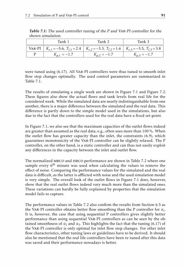
7.2 Simulation of P and Var-PI control 91
Table 7.1: The used controller tuning of the P and Var-PI controller for theshown simulation.
Tank 1 Tank 2 Tank 3
Var-PI Kc,1 =−5.6, TI,1 =2.4 Kc,2 =−3.3, TI,2 =1.6 Kc,3 =−3.5, TI,3 =3.8
P Kp,1 = −1.7 Kp,2 = −1.7 Kp,3 = −1.7
were tuned using (6.17). All Var-PI controllers were thus tuned to smooth inletflow step changes optimally. The used control parameters are summarized inTable 7.1.
The results of simulating a single week are shown in Figure 7.1 and Figure 7.2.These figures also show the actual flows and tank levels from real life for theconsidered week. While the simulated data are nearly indistinguishable from oneanother, there is a major difference between the simulated and the real data. Thisdifference is partly down to the simple model used in the simulations, but alsodue to the fact that the controllers used for the real data have a fixed set-point.
In Figure 7.1, we also see that the maximum capacities of the outlet flows indeedare greater than assumed as the real data, e.g., often uses more than 100 %. Whenthe outlet flow has greater capacity than the inlet, the constraints (6.9), whichguarantees monotonicity of the Var-PI controller can be slightly relaxed. The Pcontroller, on the other hand, is a static controller and can thus not easily exploitany differences in the capacity between the inlet and outlet flow.
The normalized mrco and isrco performance are shown in Table 7.2 where onesample every 6th minute was used when calculating the values to remove theeffect of noise. Comparing the performance values for the simulated and the realdata is difficult, as the latter is afflicted with noise and the used simulation modelis very simple. The overall look of the outlet flows in Figure 7.1 does, however,show that the real outlet flows indeed vary much more than the simulated ones.These variations can hardly be fully explained by properties that the simulationmodel fails to capture.
The performance values in Table 7.2 also confirm the results from Section 6.5 asthe Var-PI controller obtains better flow smoothing than the P controller for u1.It is, however, the case that using sequential P controllers gives slightly betterperformance than using sequential Var-PI controllers as can be seen by the ob-tained smoothness of u2 and u3. This highlights the fact that the tuning (6.17) ofthe Var-PI controller is only optimal for inlet flow step changes. For other inletflow characteristics, other tuning laws or guidelines have to be derived. It shouldalso be mentioned that the real life controllers have been re-tuned after this datawas saved and their performance nowadays is better.
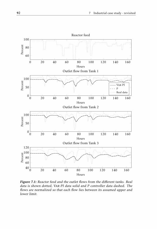
92 7 Industrial case study - revisited
0 20 40 60 80 100 120 140 1600
50
100
Hours
Perc
ent
Outlet flow from Tank 1
Var-PI
PReal data
0 20 40 60 80 100 120 140 160
60
80
100
Hours
Perc
ent
Reactor feed
0 20 40 60 80 100 120 140 1600
50
100
Hours
Perc
ent
Outlet flow from Tank 2
0 20 40 60 80 100 120 140 16040
60
80
100
120
Hours
Perc
ent
Outlet flow from Tank 3
Figure 7.1: Reactor feed and the outlet flows from the different tanks. Realdata is shown dotted, Var-PI data solid and P controller data dashed. Theflows are normalized so that each flow lies between its assumed upper andlower limit.
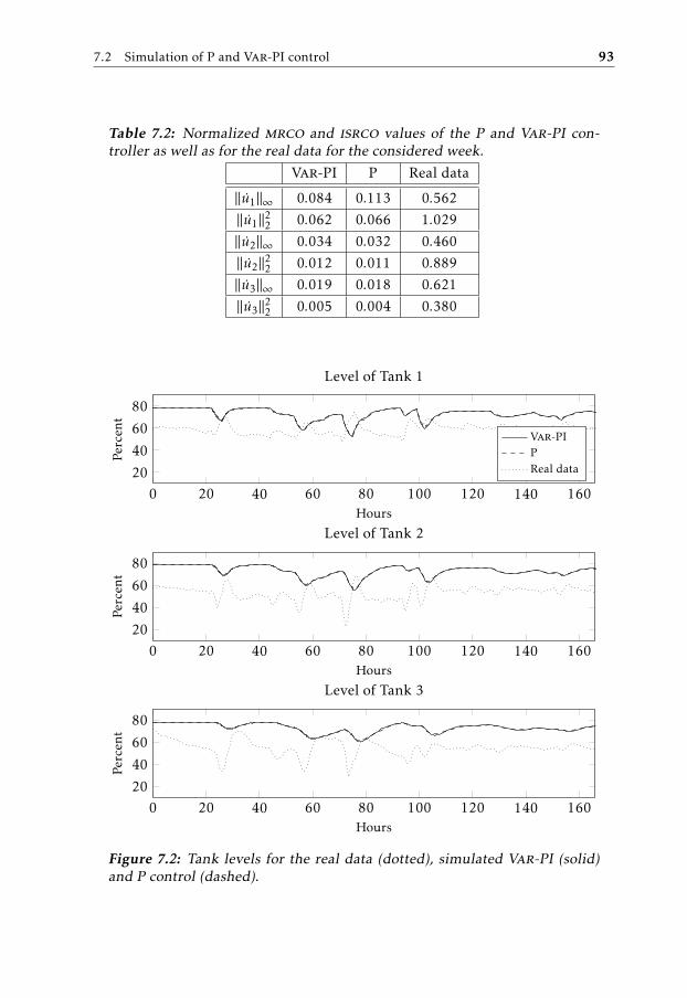
7.2 Simulation of P and Var-PI control 93
Table 7.2: Normalized mrco and isrco values of the P and Var-PI con-troller as well as for the real data for the considered week.
Var-PI P Real data
||u1||∞ 0.084 0.113 0.562
||u1||22 0.062 0.066 1.029
||u2||∞ 0.034 0.032 0.460
||u2||22 0.012 0.011 0.889
||u3||∞ 0.019 0.018 0.621
||u3||22 0.005 0.004 0.380
0 20 40 60 80 100 120 140 16020
40
60
80
Hours
Perc
ent
Level of Tank 2
0 20 40 60 80 100 120 140 16020
40
60
80
Hours
Perc
ent
Level of Tank 1
Var-PI
PReal data
0 20 40 60 80 100 120 140 16020
40
60
80
Hours
Perc
ent
Level of Tank 3
Figure 7.2: Tank levels for the real data (dotted), simulated Var-PI (solid)and P control (dashed).
94 7 Industrial case study - revisited
7.3 Flow smoothing using multiple buffer tanks
When having several buffer tanks available for flow smoothing, the achievablefiltering performance naturally increases, but so does the degrees of freedom.The question how to actually tune a specific controller naturally still remains,but with multiple tanks, also the order in which the tuning is performed has tobe considered. Furthermore, if the Var-PI controller is used, the possibility tocoordinate the set-point changes of the separate controllers also exists. Theseconsiderations will be briefly addressed and some of the issues that arise will bediscussed.
7.3.1 The order in which to perform the tuning
There exist two fundamentally different ways on how to perform the tuning ofmultiple level controllers. Either the tuning of all controllers is jointly consideredby formulating and solving an optimization problem. The other alternative is totune each controller to be locally optimal and hope that the overall performanceof the controllers are satisfying. Tuning each controller separately will indeed bemuch easier, and the only valid reason to tune the controllers jointly by solvingan optimization problem is if the achieved performance is greatly improved.
When tuning each controller individually, the natural choice is to start with themost upstream tank and then go downstream. This is because tuning a controllerrequires a description of the inlet flow which in turn requires knowledge of theupstream processes and how they are controlled. Another reason for performingthe tuning by following the process flow is that, although some flow might bemore important to keep smooth than the others, it is not likely the case that, thatshould be obtained by letting some other upstream flow vary excessively. Forexample, keeping the flow to Column 3 smooth in the Perstorp application isindeed vital but should not be obtained at the cost of a very varying outlet flowfrom, e.g., Tank 1.
7.3.2 Tuning of multiple averaging level controllers
As the simulation results in Table 7.2 show, the tuning of the Var-PI controllerhas to be extended so that it accounts for other inlet flow descriptions than a stepchange. One way would be to consider the inlet flow as a low pass filtered step
Qin(s) =1
sTq + 11s.
The tuning of the Var-PI controller would then depend on the parameter Tq,where as Tq → 0, the tuning (6.17) would be obtained.
7.3.3 Coordinating the set-point changes
One possibility when having multiple Var-PI controllers deployed closely to-gether in a sequence, is to coordinate their actions by changing their set-pointsusing the same upstream flow. In the Perstorp application, the reactor feed could,
7.4 Summarizing comments 95
for example, be used to, not only change the set-point of the controller for Tank 1,but also the succeeding two tanks. The tuning of the separate controllers shouldmost likely also account for this, making the tuning more involved. The resultingcontrol structure will also be fairly complicated. For this to be a viable approach,the performance improvement must thus be quite substantial.
7.4 Summarizing comments
There are many unsolved issues that arise when multiple buffer tanks are usedfor flow smoothing. For the Perstorp application, the most important change isprobably to change from standard PI controllers to a controller which does nothave a fixed set-point. It is rather straightforward to account for the fact thatseveral tanks are used, when performing the tuning. Other alternatives, such ascoordinating the set-point changes of the different controllers, seem less simpleto perform. All these questions remains, nonetheless, to be investigated.

8Concluding remarks
In this chapter the contributions of the thesis will be summarized and possiblefuture research directions discussed.
8.1 Conclusions
The problem of obtaining satisfactory flow filtering in the presence of frequent in-let flow changes was addressed. For a frequently changing inlet flow, individualupsets can not be treated as separate events as has previously been the case whendesigning and tuning averaging level controllers. By describing the smoothingproblem in a robust MPC framework, a controller which achieves optimal flowsmoothing while being robust towards future upsets, was obtained. The key con-cept of the robust MPC was to not return the tank level to a fixed set-point follow-ing an upset, but instead let the level vary in accordance to the value of the inletflow. This insight were used to heuristically impose robustness towards frequentflow upsets on other control structures.
Non-linear robustly optimal controllers that mimic the robust MPC were thenderived. Although perhaps not industrially applicable, they provide closed formexpressions on the achievable filtering performance for the level-adapting strat-egy that the robust MPC displays. The level-adapting behavior was also imposedon a PI controller by changing its set-point according to an affine mapping fromthe inlet flow. In a comparison with a standard P controller, which also does notreturn the level to a fixed set-point, the PI controller showed a somewhat betterfiltering performance while being less robust towards measurement noise. The PIcontroller is, however, attractive from a pedagogical perspective as its behaviorrelative to the level set-point is more intuitive than that of the P controller.
97
98 8 Concluding remarks
The filtering performance of the proposed controllers has been evaluated for bothinfrequent and frequent flow upsets. For the former, a statistical analysis showedthat the level-adapting controllers indeed achieve comparable flow smoothing asthe standard controllers even for infrequent inlet flow changes. For frequent up-sets, the controllers were evaluated by means of a simulation study using realinput data from Perstorp AB. Even though the standard controllers were opti-mally tuned for the used data set, they failed to obtain the same performance asthe proposed controllers.
8.2 Future work
The future work can be divided into two different parts. One part solely involvesthe averaging level control problem for frequent flow upsets. The other is a re-cently started project which aims to take a more comprehensive view on the useof buffer tanks and how different requirements such as, handling of stoppages,minimization of flow variations, meeting of customer demands etc. is affected by(and effects) the management of buffer tanks.
8.2.1 Averaging level control
A less computationally costly execution of the robust MPC controller can be ob-tained by using explicit MPC. Offline calculations result in a mapping from theinitial conditions of the optimization problem; the current tank level and inletflow as well as the previously actuated outlet flow, to the optimal input, u∗(0).The robust MPC can then be run with a higher sampling frequency, than if thewhole optimization problem has to be solved on-line.
Before being able to use the proposed PI controller in an industrial applicationthe question marks surrounding its sensitivity to measurement noise need to bestraightened out. The control structure should be extended with a low pass fil-ter in the mapping from inlet flow to set-point. In doing this, the controllershould also use a β factor to improve the flow smoothing. Different controllerparametrizations need to be investigated and guidelines on the tuning derived.
The assumption on equal range of the inlet and outlet flows does not hold ingeneral. The case where the outlet flow has greater capacity permits, e.g., theoutlet to have a response with a small under- or overshoot. How this affects thetuning for optimal flow performance needs to be investigated.
The use of multiple surge tanks deployed close together, with only one or a fewother processes in between them, is also an area of interest. By considering this inthe tuning of the controllers and by coordinating their action, e.g., by changingthe set-points of all controllers using the same upstream flow, the obtained flowsmoothing might be improved. For the Perstorp application the set-points toTank 2 and 3 could, for example, be given by the flow from the reactor instead ofthe actual inlet flows to the tanks. The optimal controller tuning for Tank 2 and3 also differs from the one used for Tank 1 since they do not need to surge inlet
8.2 Future work 99
flow step changes but rather the low pass filtered outlet from the first tank.
Another interesting question is to evaluate the performance criteria used to quan-tify “good flow smoothing”. The ones used in this thesis, the mrco and isrco,capture different properties of the outlet flow but the relevance these have on theperformance of the downstream processes needs to be analyzed. The answer willof course depend on the nature of the downstream processes and how they arecontrolled, but perhaps it will be possible to provide some general guidelines.
8.2.2 Buffer tank management
Buffer tanks are also used for other purposes than flow smoothing. For exam-ple, they are used to ensure fast response to customer demands or to allow forsome production even when there are stoppages. One specific case of the latter,addressed in [Lindholm, 2011], is the handling of disturbances on utilities. Forthese applications, the objective is no longer to keep the rate of the outlet flowsmall, but rather to maximize the profit or minimize the cost.
How different requirements, such as meeting a varying customer demand, han-dling of disturbances and other production stoppages, affect the buffer tank man-agement will be investigated in a recently started project between the processindustry centres at Linköping and Lund University together with Perstorp AB.

100 8 Concluding remarks
Bibliography
E.M.B. Aske. Design of plantwide control systems with focus on maximizingthroughput. PhD thesis, Norwegian University of Science and Technology,2009. Cited on page 22.
A. Ben-Tal, L. El Ghaoui, and A. Nemirovski. Robust Optimization. PrincetonUniversity Press, Oct 2009. Cited on page 34.
D.P. Bertsekas. Dynamic Programming and Optimal Control. Athena Scientific,2005. ISBN 1-886519-26-4. Cited on pages 62, 63, and 67.
S. Boyd and L. Vandenberghe. Convex Optimization. Cambridge University Press,New York, NY, USA, 2004. ISBN 0521833787. Cited on pages 33 and 35.
P.J. Campo and M. Morari. Model predictive optimal averaging level control.AIChE Journal, 35(4):579–591, Apr 1989. Cited on pages 13, 15, 48, and 58.
T. Cheung and W.L. Luyben. Liquid-level control in single tanks and cascadeof tanks with proportional-only and proportional-integral feedback control.Industrial and Engineering Chemistry Fundamentals, 18(1):15–21, Jan 1979a.Cited on pages 9, 11, 16, 17, 18, and 89.
T. Cheung and W.L. Luyben. A further study of the PL level controller. ISATransactions, 18(2):73–77, 1979b. Cited on page 19.
T. Cheung and W.L. Luyben. Nonlinear and nonconventional liquid level con-trollers. Industrial and Engineering Chemistry Fundamentals, 19(1):93–98,1980. Cited on page 19.
P.J. Goulart, E.C. Kerrigan, and J.M. Maciejowsky. Optimization over state feed-back policies for robust control with constraints. Automatica, 42(4):523–533,Apr 2006. Cited on page 38.
R.W. Hamming. Numerical methods for scientists and engineers. Dover Publi-cations, Inc., New York, NY, USA, 1973. ISBN 0-486-65241-6. Cited on page2.
101
102 Bibliography
E.C. Horton, M.W. Foley, and K.E. Kwok. Performance assessment of level con-trollers. Internation journal of adaptive control and signal processing, 17(7-9):663–684, Sep-Nov 2003. Cited on page 8.
J.D. Kelly. Tuning digital PI controllers for minimal variance in manipulatedinput moves applied to imbalanced systems with delay. Canadian Journal ofChemical Engineering, 76(5):967–974, Oct 1998. Cited on page 8.
M. Khanbaghi, B. Allison, and R. Harper. Optimal averaging level control forsurge tanks. In IEEE Conference on Advanced Process Control Applicationsfor Industry, Vancouver, Canada, 2001. Cited on page 6.
B-M Kwon, M-E Lee, and O-K Kwon. On nonovershooting of monotone nonde-creasing step response of second-order systems. Transactions on Control, Au-tomation and Systems Engingeering, 4(4):283–288, Dec 2002. Cited on page75.
M. Lee and J. Shin. Constrained optimal control of liquid level loop using aconventional proportional-integral controller. Chemical Engineering Comm.,196(6):729–745, Jan 2009. Cited on pages 9, 10, and 11.
A. Lindholm. Utility disturbance management in the process industry. LicentiateThesis ISRN LUTFD2/TFRT--3253--SE, October 2011. Cited on page 99.
J. Löfberg. Approximations of closed-loop minimax MPC. In Proceedings of the42nd Conference on Decicion and Control, Maui, USA, Dec 2003. Cited onpage 37.
J. Löfberg. Yalmip : A toolbox for modeling and optimization in MATLAB. InProceedings of the CACSD Conference, Taipei, Taiwan, 2004. URL http://users.isy.liu.se/johanl/yalmip. Cited on page 41.
J. Löfberg. Automatic robust convex programming. Optimization Methods andSoftware, 27(1):115–129, 2012. Cited on pages 34, 35, 39, and 40.
W.L. Luyben and P.S. Buckley. A proportional-lag level controller. Instrumenta-tion Technology, 18(1):65–68, 1977. Cited on page 19.
J.M. Maciejowski. Predictive Control with Constraints. Prentice Hall, 1st edition,2002. ISBN 0201398230. Cited on pages 31 and 33.
D.Q. Mayne, J.B. Rawlings, C.V. Rao, and P.O.M. Scokaert. Constrained modelpredictive control: Stability and optimality. Automatica, 36(6):789–814, Jun2000. Cited on page 32.
K.A. McDonald, T.J. McAvoy, and A. Tits. Optimal averaging level control. AIChEJournal, 32(1):75–86, Jan 1986. Cited on pages 6, 12, 55, 57, and 64.
S. Ogawa. Stochastic Averaging Level Contol and Its Application to Broke Man-agement in Paper Machines. PhD thesis, The University of British Columbia,2003. Cited on page 19.
Bibliography 103
P. Rosander, A.J. Isaksson, J. Löfberg, and K. Forsman. Robust averaging levelcontrol. In Proccedings of the 2011 AIChE Annual Meeting, Minneapolis,USA,2011. Cited on page 31.
P. Rosander, A.J. Isaksson, J. Löfberg, and K. Forsman. Performace analysis ofrobust averaging level control. In Proceedings of Chemical Process ControlVIII, Savannah, USA, 2012a. Cited on page 55.
P. Rosander, A.J. Isaksson, J. Löfberg, and K. Forsman. Practical control of surgetanks suffering from frequent inlet flow upsets. In Proceedings of the IFACConference on Advances in PID Control, Brescia, ITA, 2012b. Cited on page 71.
J. Shin, J. Lee, S. Park, K. Koo, and M. Lee. Analytical design of a proportional-integral controller for constrained optimal regulatory control of inventory loop.Control Engineering Practice, 16(11):1391–1397, Nov 2008. Cited on page 10.
J.P. Shunta and W. Fehervari. Nonlinear control of liquid-level. InstrumentationTechnology, 23(1):43–48, Jan 1976. Cited on page 19.
A.J. Taylor and T.G. la Grange. Optimize surge vessel control - proportional onlyalgorithm complements multivariable predictive control. Hydrocarbon Pro-cessing, 81(5):49–52, May 2002. Cited on pages 16 and 17.
M. Tharayil and A. Alleyne. A generalized PID error governing scheme forSMART/SBLI control. In Proceedings of the American Control Conference,2002, 2002. Cited on page 81.
K.L. Wu, C.C. Yu, and Y.C. Cheng. A two degree of freedom level control. Journalof Process Control, 11(3):311–319, Jun 2001. Cited on page 19.
W. Yin. Gurobi Mex: A MATLAB interface for Gurobi, 2009-2011.URL http://convexoptimization.com/wikimization/index.php/gurobi_mex. Cited on page 41.

Licentiate ThesesDivision of Automatic Control
Linköping UniversityP. Andersson: Adaptive Forgetting through Multiple Models and Adaptive Control of CarDynamics. Thesis No. 15, 1983.B. Wahlberg: On Model Simplification in System Identification. Thesis No. 47, 1985.A. Isaksson: Identification of Time Varying Systems and Applications of System Identifi-cation to Signal Processing. Thesis No. 75, 1986.G. Malmberg: A Study of Adaptive Control Missiles. Thesis No. 76, 1986.S. Gunnarsson: On the Mean Square Error of Transfer Function Estimates with Applica-tions to Control. Thesis No. 90, 1986.M. Viberg: On the Adaptive Array Problem. Thesis No. 117, 1987.
K. Ståhl: On the Frequency Domain Analysis of Nonlinear Systems. Thesis No. 137, 1988.A. Skeppstedt: Construction of Composite Models from Large Data-Sets. Thesis No. 149,1988.P. A. J. Nagy: MaMiS: A Programming Environment for Numeric/Symbolic Data Process-ing. Thesis No. 153, 1988.K. Forsman: Applications of Constructive Algebra to Control Problems. Thesis No. 231,1990.I. Klein: Planning for a Class of Sequential Control Problems. Thesis No. 234, 1990.F. Gustafsson: Optimal Segmentation of Linear Regression Parameters. Thesis No. 246,1990.H. Hjalmarsson: On Estimation of Model Quality in System Identification. Thesis No. 251,1990.S. Andersson: Sensor Array Processing; Application to Mobile Communication Systemsand Dimension Reduction. Thesis No. 255, 1990.K. Wang Chen: Observability and Invertibility of Nonlinear Systems: A Differential Alge-braic Approach. Thesis No. 282, 1991.J. Sjöberg: Regularization Issues in Neural Network Models of Dynamical Systems. ThesisNo. 366, 1993.P. Pucar: Segmentation of Laser Range Radar Images Using Hidden Markov Field Models.Thesis No. 403, 1993.H. Fortell: Volterra and Algebraic Approaches to the Zero Dynamics. Thesis No. 438,1994.T. McKelvey: On State-Space Models in System Identification. Thesis No. 447, 1994.T. Andersson: Concepts and Algorithms for Non-Linear System Identifiability. ThesisNo. 448, 1994.P. Lindskog: Algorithms and Tools for System Identification Using Prior Knowledge. The-sis No. 456, 1994.J. Plantin: Algebraic Methods for Verification and Control of Discrete Event DynamicSystems. Thesis No. 501, 1995.J. Gunnarsson: On Modeling of Discrete Event Dynamic Systems, Using Symbolic Alge-braic Methods. Thesis No. 502, 1995.A. Ericsson: Fast Power Control to Counteract Rayleigh Fading in Cellular Radio Systems.Thesis No. 527, 1995.M. Jirstrand: Algebraic Methods for Modeling and Design in Control. Thesis No. 540,1996.K. Edström: Simulation of Mode Switching Systems Using Switched Bond Graphs. ThesisNo. 586, 1996.
J. Palmqvist: On Integrity Monitoring of Integrated Navigation Systems. Thesis No. 600,1997.A. Stenman: Just-in-Time Models with Applications to Dynamical Systems. ThesisNo. 601, 1997.M. Andersson: Experimental Design and Updating of Finite Element Models. ThesisNo. 611, 1997.U. Forssell: Properties and Usage of Closed-Loop Identification Methods. Thesis No. 641,1997.M. Larsson: On Modeling and Diagnosis of Discrete Event Dynamic systems. ThesisNo. 648, 1997.N. Bergman: Bayesian Inference in Terrain Navigation. Thesis No. 649, 1997.V. Einarsson: On Verification of Switched Systems Using Abstractions. Thesis No. 705,1998.J. Blom, F. Gunnarsson: Power Control in Cellular Radio Systems. Thesis No. 706, 1998.P. Spångéus: Hybrid Control using LP and LMI methods – Some Applications. ThesisNo. 724, 1998.M. Norrlöf: On Analysis and Implementation of Iterative Learning Control. ThesisNo. 727, 1998.A. Hagenblad: Aspects of the Identification of Wiener Models. Thesis No. 793, 1999.
F. Tjärnström: Quality Estimation of Approximate Models. Thesis No. 810, 2000.C. Carlsson: Vehicle Size and Orientation Estimation Using Geometric Fitting. ThesisNo. 840, 2000.J. Löfberg: Linear Model Predictive Control: Stability and Robustness. Thesis No. 866,2001.O. Härkegård: Flight Control Design Using Backstepping. Thesis No. 875, 2001.J. Elbornsson: Equalization of Distortion in A/D Converters. Thesis No. 883, 2001.J. Roll: Robust Verification and Identification of Piecewise Affine Systems. Thesis No. 899,2001.I. Lind: Regressor Selection in System Identification using ANOVA. Thesis No. 921, 2001.
R. Karlsson: Simulation Based Methods for Target Tracking. Thesis No. 930, 2002.P.-J. Nordlund: Sequential Monte Carlo Filters and Integrated Navigation. Thesis No. 945,2002.M. Östring: Identification, Diagnosis, and Control of a Flexible Robot Arm. ThesisNo. 948, 2002.C. Olsson: Active Engine Vibration Isolation using Feedback Control. Thesis No. 968,2002.J. Jansson: Tracking and Decision Making for Automotive Collision Avoidance. ThesisNo. 965, 2002.N. Persson: Event Based Sampling with Application to Spectral Estimation. ThesisNo. 981, 2002.D. Lindgren: Subspace Selection Techniques for Classification Problems. Thesis No. 995,2002.E. Geijer Lundin: Uplink Load in CDMA Cellular Systems. Thesis No. 1045, 2003.
M. Enqvist: Some Results on Linear Models of Nonlinear Systems. Thesis No. 1046, 2003.
T. Schön: On Computational Methods for Nonlinear Estimation. Thesis No. 1047, 2003.F. Gunnarsson: On Modeling and Control of Network Queue Dynamics. Thesis No. 1048,2003.S. Björklund: A Survey and Comparison of Time-Delay Estimation Methods in LinearSystems. Thesis No. 1061, 2003.
M. Gerdin: Parameter Estimation in Linear Descriptor Systems. Thesis No. 1085, 2004.
A. Eidehall: An Automotive Lane Guidance System. Thesis No. 1122, 2004.E. Wernholt: On Multivariable and Nonlinear Identification of Industrial Robots. ThesisNo. 1131, 2004.J. Gillberg: Methods for Frequency Domain Estimation of Continuous-Time Models. The-sis No. 1133, 2004.G. Hendeby: Fundamental Estimation and Detection Limits in Linear Non-Gaussian Sys-tems. Thesis No. 1199, 2005.D. Axehill: Applications of Integer Quadratic Programming in Control and Communica-tion. Thesis No. 1218, 2005.J. Sjöberg: Some Results On Optimal Control for Nonlinear Descriptor Systems. ThesisNo. 1227, 2006.D. Törnqvist: Statistical Fault Detection with Applications to IMU Disturbances. ThesisNo. 1258, 2006.H. Tidefelt: Structural algorithms and perturbations in differential-algebraic equations.Thesis No. 1318, 2007.S. Moberg: On Modeling and Control of Flexible Manipulators. Thesis No. 1336, 2007.J. Wallén: On Kinematic Modelling and Iterative Learning Control of Industrial Robots.Thesis No. 1343, 2008.J. Harju Johansson: A Structure Utilizing Inexact Primal-Dual Interior-Point Method forAnalysis of Linear Differential Inclusions. Thesis No. 1367, 2008.J. D. Hol: Pose Estimation and Calibration Algorithms for Vision and Inertial Sensors.Thesis No. 1370, 2008.H. Ohlsson: Regression on Manifolds with Implications for System Identification. ThesisNo. 1382, 2008.D. Ankelhed: On low order controller synthesis using rational constraints. ThesisNo. 1398, 2009.P. Skoglar: Planning Methods for Aerial Exploration and Ground Target Tracking. ThesisNo. 1420, 2009.C. Lundquist: Automotive Sensor Fusion for Situation Awareness. Thesis No. 1422, 2009.C. Lyzell: Initialization Methods for System Identification. Thesis No. 1426, 2009.R. Falkeborn: Structure exploitation in semidefinite programming for control. ThesisNo. 1430, 2010.D. Petersson: Nonlinear Optimization Approaches toH2-Norm Based LPV Modelling andControl. Thesis No. 1453, 2010.Z. Sjanic: Navigation and SAR Auto-focusing in a Sensor Fusion Framework. ThesisNo. 1464, 2011.K. Granström: Loop detection and extended target tracking using laser data. ThesisNo. 1465, 2011.J. Callmer: Topics in Localization and Mapping. Thesis No. 1489, 2011.F. Lindsten: Rao-Blackwellised particle methods for inference and identification. ThesisNo. 1480, 2011.M. Skoglund: Visual Inertial Navigation andCalibration. Thesis No. 1500, 2011.
S. Khoshfetrat Pakazad: Topics in Robustness Analysis. Thesis No. 1512, 2011.
P. Axelsson: On Sensor Fusion Applied to Industrial Manipulators. Thesis No. 1511, 2011.A. Carvalho Bittencourt: On Modeling and Diagnosis of Friction and Wear in IndustrialRobots. Thesis No. 1516, 2012.