Embed Size (px)
Citation preview

F i n a l R e p o r t
LOWERMOOR
WATER QUALITY MODELLING REPORT (Phase 2)
August 2006

Department of Health Lowermoor Water Quality Modelling Report (Phase 2)
Black & Veatch Ltd Appendix 13 B&V Report Phase 2 (i)
LOWERMOOR WATER QUALITY MODELLING REPORT (PHASE 2)
CONTENTS
1. BACKGROUND 1
2. MODELLING METHOD 1 2.1 Sources of model information ....................................................................................... 2 2.2 Contact tank model setup .............................................................................................. 3 2.3 Clear water tank model setup ........................................................................................ 4 2.4 Distribution network model setup ................................................................................. 6
3. RESULTS 8 3.1 Contact tank ................................................................................................................... 8 3.2 Clear water tank ........................................................................................................... 14 3.3 Distribution system ...................................................................................................... 17
4. INFLUENCE OF SLUDGE IN CONTACT TANK 20 4.1 Sludge cause and characteristics ................................................................................. 20 4.2 Likelihood of sludge in the contact tank ..................................................................... 21 4.3 Model of contact tank with sludge deposits ................................................................ 22 4.4 Model results with sludge present ............................................................................... 23
5. ANALYSIS AND DISCUSSION 28 5.1 Effect of Aluminium sulphate on pH in the Contact Tank ......................................... 28 5.2 Comparison of sample data with model predictions ................................................... 30 5.3 Model accuracy ............................................................................................................ 39 5.4 Response to specific questions from the Committee .................................................. 41
6. CONCLUSIONS 43
REFERENCES AND INFORMATION SOURCES 44
Document issue details:
BV project no. 107986 Client’s reference no.
Version no. Issue date Issue status Distribution
1 30/08/06 Draft F Pollitt (DH), MJB
2 07/09/06 Final F Pollitt (DH), MJB
3 16/03/07 Final Rev. A F Pollitt (DH), MJB
Notice:
This report was prepared by Black & Veatch Limited (BVL) solely for use by The Department of Health (DH). This report is not addressed to and may not be relied upon by any person or entity other than DH for any purpose without the prior written permission of BVL. BVL, its directors, employees and affiliated companies accept no responsibility or liability for reliance upon or use of this report (whether or not permitted) other than by DH for the purposes for which it was originally commissioned and prepared.
In producing this report, BVL has relied upon information provided by others. The completeness or accuracy of this information is not guaranteed by BVL.

Department of Health Lowermoor Water Quality Modelling Report (Phase 2)
Black & Veatch Ltd Appendix 13 B&V Report Phase 2 (ii)
FIGURES
Figure 1 Flows and water level in clear water tank ................................................................ 3 Figure 2 Layout of contact tank as modelled ......................................................................... 3 Figure 3 Mesh for contact tank model .................................................................................... 4 Figure 4 Plan of reservoir model ............................................................................................ 5 Figure 5 3D view of clear water tank ..................................................................................... 5 Figure 6 3D view of clear water tank mesh ............................................................................ 5 Figure 7 Extent of Lowermoor network model ...................................................................... 7 Figure 8 Streamlines for flow through tank at time zero ........................................................ 8 Figure 9 Predicted Al concentration in contact tank at 37 minutes ........................................ 9 Figure 10 Cut showing mixing at hole in old wall at 37 minutes ............................................. 9 Figure 11 Predicted Al concentration in contact tank 5 to 50 minutes ................................... 10 Figure 12 Predicted Al concentration in contact tank 1 to 4.5 hours ..................................... 11 Figure 13 Predicted Al concentration along final lane of contact tank .................................. 12 Figure 14 Predicted Al concentration after 37 minutes at various heights ............................. 13 Figure 15 Predicted Al concentration at contact tank outlet ................................................... 14 Figure 16 Streamlines for flow through clear water tank ....................................................... 14 Figure 17 Predicted Al concentration in reservoir at 3 hours ................................................. 15 Figure 18 Predicted Al concentration in clear water tank 1 to 11 hours ................................ 16 Figure 19 Predicted Al concentration at clear water tank outlet ............................................ 17 Figure 20 Assumed profile of compacted sludge ................................................................... 22 Figure 21 Predicted Al concentration in contact tank with and without sludge ..................... 24 Figure 22 Predicted Al concentration at contact tank outlet with and without sludge ........... 25 Figure 23 Predicted Al concentration in clear water tank with and without sludge ............... 26 Figure 24 Predicted Al concentration at clear water tank outlet with and without sludge ..... 27 Figure 25 pH versus Alum dose ............................................................................................. 29 Figure 26 Predicted propagation of Al through trunk mains .................................................. 31 Figure 27 Predicted Al concentration on trunk mains in Camelford ...................................... 32 Figure 28 Predicted Al concentration on trunk mains in St Teath ......................................... 33 Figure 29 Predicted Al concentration on trunk mains - Helstone and Michaelstow res. ....... 34 Figure 30 Predicted Al concentration on trunk mains in Port Isaac and St Endellion ........... 35 Figure 31 Predicted Al concentration on trunk mains in Delabole reservoir area .................. 36 Figure 32 Predicted Al concentration on trunk mains in Rockhead reservoir area ................ 37 Figure 33 Predicted Al concentration on trunk mains in Davidstow reservoir area ............... 38 Figure 34 Comparison of CFD prediction with simple spreadsheet models .......................... 40
TABLES
Table 1 Predicted age of water before incident (5th) and when flushing system (7th) ....... 18 Table 2 Predicted maximum contaminant concentration .................................................... 19 Table 3 Predicted maximum contaminant concentration with sludge in contact tank ........ 28 Table 4 Typical Lowermoor WTW raw water quality in 1988 and calculated doses ......... 29 Table 5 Sample data for Camelford area ............................................................................. 32 Table 6 Sample data for St Teath area ................................................................................ 33 Table 7 Sample data for Helstone and Michaelstow reservoir area .................................... 34 Table 8 Sample data for Port Issac area .............................................................................. 35 Table 9 Sample data for St Endellion area .......................................................................... 36 Table 10 Sample data for Delabole reservoir area ................................................................ 36 Table 11 Sample data for Rockhead reservoir inlet .............................................................. 37 Table 12 Sample data for Rockhead reservoir supply area ................................................... 38 Table 13 Sample data for Davidstow reservoir area ............................................................. 39
Department of Health Lowermoor Water Quality Modelling Report (Phase 2)
Black & Veatch Ltd Appendix 13 B&V Report Phase 2 (1)
LOWERMOOR WATER QUALITY MODELLING REPORT (PHASE 2)
1. BACKGROUND
The Lowermoor water pollution incident occurred on 6 July 1988 after a tanker full of aluminium sulphate was wrongly discharged into the last compartment of the contact tank at Lowermoor water treatment works. The aluminium sulphate mixed in that tank and the diluted contaminant transferred into the clear water tank on the site. Further mixing took place in this second tank prior to the water entering the distribution system. The area supplied, herein referred to as the “Lowermoor supply zone”, includes; Tintagel, Boscastle, Marshgate and Otterham (to the north and east); Camelford, Slaughterbridge, Delabole, St Teath and Michaelstow (east of the works); and Port Isaac and St Endellion (to the west).
In January 2004, the Department of Health (DH) asked Black & Veatch (B&V) to undertake a technical audit of reports prepared by Crowther Clayton Associates which summarised conclusions from two water quality models of the incident. Following a brief review of the reports B&V concluded that the reports did not fully address either the mixing and dispersion of the aluminium sulphate in the tanks at the treatment works or the time lag as the contaminated water propagated through the distribution system. Both of these factors would impact on the duration of the incident and the exposure level to the public. B&V was subsequently asked to address both points using water quality modelling tools and techniques. The purpose of the analysis was therefore to supplement the committee’s understanding of the potential contaminant concentration and duration of exposure by modelling the two storage facilities at Lowermoor to quantify the time variable concentration of pollutant leaving the works and the spread of the incident through the distribution network.
An employee of South West Water Authority at the time of the incident is reported as stating that the bottom of the contact tank was filled to the level of the outlet pipe with a solid compacted deposit of sludge (Reference 14). This conflicts with other information, but if correct it would have a significant influence on the concentration of aluminium sulphate entering the network. Subsequent to B&V’s initial report (October 2004), the committee has requested further modelling work to assess the potential implications of a build up of “solid compacted sludge” within the contact tank. This report is an update of the original report to include this additional analysis.
2. MODELLING METHOD
The methodology used in this study was to analyse each component of the system in turn using the output of the upstream component as the input for the next component:
• Model of contact tank • Model of clear water tank • Model of distribution network (trunk mains only)
The dilution effect within the pipe connecting the contact and clear water tanks was ignored because it was considered negligible compared with the dilution and dispersion taking place within the two tanks.
All the models assume that the aluminium remains in solution and does not react with other compounds (i.e. it is a conservative chemical).
As with any modelling method, there are limitations with the accuracy of results. All models are a simplification of true behaviour and their accuracy is inherently limited by the accuracy and completeness of the information used to build the model. Model accuracy is discussed further in Section 5.3.

Department of Health Lowermoor Water Quality Modelling Report (Phase 2)
Black & Veatch Ltd Appendix 13 B&V Report Phase 2 (2)
2.1 Sources of model information
The reference and data sources used in this study are listed at the end of this report.
2.1.1 Contact tank details
A record drawing was available for the contact tank (Reference 1). The tank was converted from a reservoir to a contact tank in about 1972. Since it was not originally designed as a contact tank, its performance is unlikely to be as efficient as a purpose built contact tank. With the exception of the clarifications described below, the structure dimensions, top water levels and pipe work arrangements at the time of the incident have been assumed to be as shown on the drawing. South West Water (SWW) provided additional information in July 2004 relating directly to:
• The construction of the baffle walls within the contact tank: The baffles extend to the full depth of the tank. This will have a significant impact on the dispersion of the pollutant within the tank.
• The contact tank outlet: The outlet is at high not at low level as previously reported.
2.1.2 Clear water tank details
A record drawing was available for the clear water tank (Reference 2). There was confusion and doubt about the inlet “structure” and its performance, but it has been confirmed by SWW that the tank inlet is a bellmouth discharging above the storage top water level as indicated on the drawing.
2.1.3 Distribution network
In 1993, B&V created a computer hydraulic model (Stoner software) of the storage and trunk main distribution systems for the system supplying the Lowermoor supply zone which included the Lowermoor water treatment works. Although the hydraulic model represented a more recent operational supply scenario, it was a conversion from an earlier model (WATNET software) and included information that identified some of the changes made since 1988. B&V concluded that in the absence of any better information this model could be modified to produce a reasonable representation of conditions in July 1988.
2.1.4 Flow data
A critical data input for all three models is the flow rate. In 1988 water passed from the contact tank, into which the aluminium sulphate was discharged, into the clear water tank and thence into distribution. The feed through the contact tank and into the clear water tank was dictated by the flow rate through the treatment works. The discharge from the clear water tank was dictated by the demand (consumption) of water within the distribution system. The difference between the clear water tank inflow and outflow was accounted for by variation in water level in the tank. A chart recording (Reference 5) was available for the flow through the treatment works (flow through contact tank and into the clear water tank). Another chart recording (Reference 6) was available for the water level in the clear water tank. From these two sets of data, the outflow from the clear water tank (inflow into distribution) has been calculated. Figure 1 illustrates the hourly flow profile and water level in the clear water tank between 6th July and 11th July 1988.

Department of Health Lowermoor Water Quality Modelling Report (Phase 2)
Black & Veatch Ltd Appendix 13 B&V Report Phase 2 (3)
0
20
40
60
80
100
120
140
160
Tue 05 Jul00:00
Wed 06 Jul00:00
Thu 07 Jul00:00
Fri 08 Jul00:00
Sat 09 Jul00:00
Sun 10 Jul00:00
Mon 11 Jul00:00
Flow
(L/s
)
0.0
0.4
0.8
1.2
1.6
2.0
2.4
2.8
3.2
Res
Dep
th (m
)
Flow In (L/s) Flow Out (L/s) Res Level (m)
Figure 1 Flows and water level in clear water tank
In order to model the contact tank and reservoir, the flow into the treatment works was simplified as given below:
Model Time Actual time Flow Reference 0 to 0.33 hr 17:00 – 17:20 63L/s (Reference 5 & 10) 0.33 to 2hr 17:20 – 19:00 61L/s (Reference 5 & 10) 2 to 7hr 19:00 – 00:00 54L/s (Reference 5) 7 to 19hr 00:00 – 12:00 79L/s (Reference 5) 19 to 24hr 12:00 – 17:00 76L/s (Reference 5)
2.2 Contact tank model setup
The contact tank was analysed using computational fluid dynamics (CFD) software which simulated the three dimensional hydraulics and dispersion of aluminium sulphate. The model assumes that the aluminium remains in solution and does not react with other compounds (i.e. it is a conservative chemical). The model represents the full geometry of the tank, the flow regime during the incident and the injection of the pollutant through the inspection cover at the upstream end of the final lane. The layout of the contact tank as modelled is shown in Figure 2 with the basic flow path shown by the blue arrows.
Figure 2 Layout of contact tank as modelled
Plan view 3D view

Department of Health Lowermoor Water Quality Modelling Report (Phase 2)
Black & Veatch Ltd Appendix 13 B&V Report Phase 2 (4)
Details of the model set up are given below (original simulation without sludge in contact tank):
• Flow into tank: As explained in Section 2.1.4 above • Pollutant details:
- 8% aluminium sulphate, equivalent to 56,000 mg/l Al - Density of 1.32 kg/L. - Discharge duration 37 min starting at 17:00hrs (time zero) - Discharge rate 6.82 L/s (Reference DH letter dated 14 April 2004).
• Simulation details – model without sludge in tank: - Software: CFX version 5.7 - Steady state analysis of hydraulics only at time zero to give start conditions. - Transient analysis 0 to 4.5 hrs - Turbulence simulated using a k-ε model - Mesh size: 702,000 unstructured tetrahedral elements with an inflated boundary
for more accurate modelling of the influence of walls. The mesh for the model is shown in Figure 3. This relatively fine mesh was specifically refined around the inlet, outlet and the hatch through which the aluminium sulphate was discharged since these are the regions of the model in which there is most hydraulic activity.
This was a detailed model which took over two weeks to run on a high power (twin 2.7 Ghz) computer.
Figure 3 Mesh for contact tank model
2.3 Clear water tank model setup
The reservoir was analysed using a CFD model which simulated the three dimensional hydraulics and dispersion of aluminium sulphate. The model assumes that the aluminium remains in solution and does not react with other compounds. In order to enable simulation of a full 24hr period, the level of detail in this model is lower than that used for the contact tank. However, this is a reasonable approach since:
• It is a simpler structure without baffles and internal constrictions • The velocities are lower, so adjacent elements in the model tend to have similar values • The concentrations are lower, so adjacent elements in the model tend to have similar
values

Department of Health Lowermoor Water Quality Modelling Report (Phase 2)
Black & Veatch Ltd Appendix 13 B&V Report Phase 2 (5)
Details of the model set up are given below:
• Flow into tank: As explained in Section 2.1.4 above • Water level: The water level was simplified in the model as follows:
Model Time Actual time Level 0 to 11hr 17:00 – 04:00 2.2m 11 to 15hr 04:00 – 08:00 2.2 falling to 1.3m (constant rate) 15 to 24hr 08:00 – 17:00 1.3m
• Pollutant details: - Properties as for contact tank - Concentration entering the tank as given by the preceding analysis of the contact
tank • Simulation details:
- Software: CFX version 5.7 - Steady state analysis of hydraulics only at time zero to give start conditions. - Transient analysis 0 to 24 hr - Turbulence simulated using a k-ε model - Mesh size – 0 to 11 hr: 393, 000 elements (medium quality) - Mesh size – 11 to 24 hr: 154,000 elements (coarse quality) with moving mesh to
simulate change in water level.
A plan of the layout modelled is shown in Figure 4. A 3D representation of the model and the mesh is given in Figure 5 and Figure 6.
Figure 4 Plan of reservoir model
Figure 5 3D view of clear water tank Figure 6 3D view of clear water tank mesh
Department of Health Lowermoor Water Quality Modelling Report (Phase 2)
Black & Veatch Ltd Appendix 13 B&V Report Phase 2 (6)
2.4 Distribution network model setup
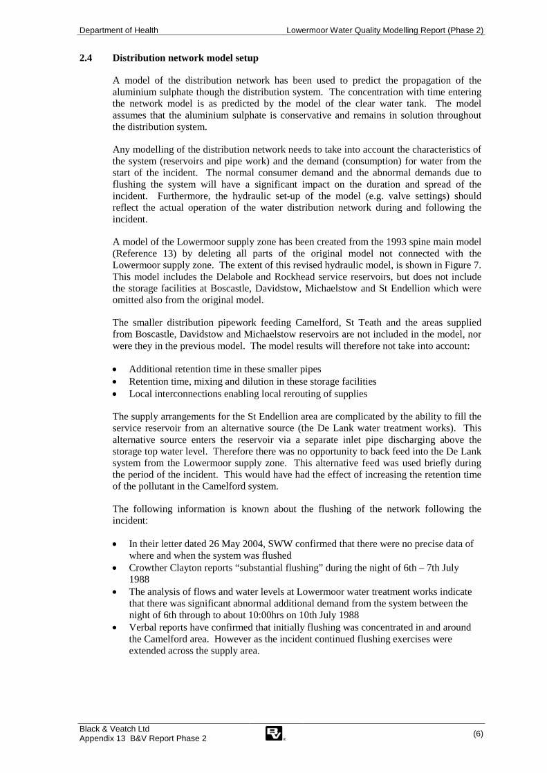
A model of the distribution network has been used to predict the propagation of the aluminium sulphate though the distribution system. The concentration with time entering the network model is as predicted by the model of the clear water tank. The model assumes that the aluminium sulphate is conservative and remains in solution throughout the distribution system.
Any modelling of the distribution network needs to take into account the characteristics of the system (reservoirs and pipe work) and the demand (consumption) for water from the start of the incident. The normal consumer demand and the abnormal demands due to flushing the system will have a significant impact on the duration and spread of the incident. Furthermore, the hydraulic set-up of the model (e.g. valve settings) should reflect the actual operation of the water distribution network during and following the incident.
A model of the Lowermoor supply zone has been created from the 1993 spine main model (Reference 13) by deleting all parts of the original model not connected with the Lowermoor supply zone. The extent of this revised hydraulic model, is shown in Figure 7. This model includes the Delabole and Rockhead service reservoirs, but does not include the storage facilities at Boscastle, Davidstow, Michaelstow and St Endellion which were omitted also from the original model.
The smaller distribution pipework feeding Camelford, St Teath and the areas supplied from Boscastle, Davidstow and Michaelstow reservoirs are not included in the model, nor were they in the previous model. The model results will therefore not take into account:
• Additional retention time in these smaller pipes • Retention time, mixing and dilution in these storage facilities • Local interconnections enabling local rerouting of supplies
The supply arrangements for the St Endellion area are complicated by the ability to fill the service reservoir from an alternative source (the De Lank water treatment works). This alternative source enters the reservoir via a separate inlet pipe discharging above the storage top water level. Therefore there was no opportunity to back feed into the De Lank system from the Lowermoor supply zone. This alternative feed was used briefly during the period of the incident. This would have had the effect of increasing the retention time of the pollutant in the Camelford system.
The following information is known about the flushing of the network following the incident:
• In their letter dated 26 May 2004, SWW confirmed that there were no precise data of where and when the system was flushed
• Crowther Clayton reports “substantial flushing” during the night of 6th – 7th July 1988
• The analysis of flows and water levels at Lowermoor water treatment works indicate that there was significant abnormal additional demand from the system between the night of 6th through to about 10:00hrs on 10th July 1988
• Verbal reports have confirmed that initially flushing was concentrated in and around the Camelford area. However as the incident continued flushing exercises were extended across the supply area.

Department of Health Lowermoor Water Quality Modelling Report (Phase 2)
Black & Veatch Ltd Appendix 13 B&V Report Phase 2 (7)
Figure 7 Extent of Lowermoor network model
Model (trunk mains only)
Network map (excludes Delabole to St Endellion mains) Blue indicates mains included in model

Department of Health Lowermoor Water Quality Modelling Report (Phase 2)
Black & Veatch Ltd Appendix 13 B&V Report Phase 2 (8)
In the light of this information, the demands in the Lowermoor hydraulic model have been derived from actual flow data recorded between 5 and 11 July 1988 as detailed below:
• The water consumed within the network was separated into two categories (1) consumer demand, and (2) flushing demand
• The consumer demand profile for the full period was assumed to equal the full flow profile into the network recorded on the day before the incident
• The spatial distribution of consumer demand is assumed to be as in the previous model of the area
• The flushing demand profile was calculated by subtracting the consumer demand from the overall flow into the network. Occasionally this returned a small negative value in which case zero flushing demand was assumed for that time-step.
• The flushing flow has been assigned to the Camelford area during the night of 6/7 July and into the morning of the 7th. Thereafter flushing has been assumed to be more widespread and has been distributed proportional to all demand centres in the model.
The concentration curve derived for the clear water tank outlet using CFD modelling (Section 2.3) was assigned as an inlet boundary condition in the network model.
3. RESULTS
3.1 Contact tank
Figure 8 shows the predicted streamlines for the flow through the tank immediately prior to the discharge of aluminium sulphate. Each blue line is the path taken by a small parcel of water entering at the inlet. The figure shows swirling flow around the inlet and the holes in the wall but on entering the last leg, the baffles have straightened out the flow path. This behaviour is as would be anticipated, giving confidence in the model predictions. The more swirling the flow the greater the mixing that will occur.
Figure 8 Streamlines for flow through tank at time zero
Figure 9 shows the predicted aluminium concentrations throughout the contact tank after 37 minutes of aluminium sulphate being discharged into the tank. This is just before the tanker completed discharging and so represents the peak quantity of aluminium sulphate within the tank. The multicoloured planes in Figure 9 indicate the predicted concentration on cuts along the lanes in the tank. The colour coding is quantified by the legend adjacent to the figure:
3D view
Plan view

Department of Health Lowermoor Water Quality Modelling Report (Phase 2)
Black & Veatch Ltd Appendix 13 B&V Report Phase 2 (9)
• Dark blue: Regions of low concentration • Green: 1,000 to 2,000 mg/L Al • Yellow / orange / red: 2,000 to 3,000 mg/L Al • Dark red: In excess of 3,000 mg/L Al
The model predicts that the aluminium sulphate did not mix rapidly with the water in the tank, and sank to the base. It then spread out along the base of the tank in all directions. Some of the aluminium sulphate spread against the principle flow direction until it reached the holes in the old wall. Here the velocity of flow is much higher causing the aluminium sulphate to be mixed up into the bulk flow (Figure 10). A small amount of aluminium sulphate spread through both the holes back to the tank inlet. It is this relatively small proportion of the aluminium sulphate which would have triggered the pH alarm.
Figure 9 Predicted Al concentration in contact tank at 37 minutes
Figure 10 Cut showing mixing at hole in old wall at 37 minutes

Department of Health Lowermoor Water Quality Modelling Report (Phase 2)
Black & Veatch Ltd Appendix 13 B&V Report Phase 2 (10)
The progressive build up and release with time of aluminium sulphate in the tank is shown by Figure 11 and Figure 12. Time zero is the start of the discharge (approximately 17:00).
5 minutes
10 minutes
20 minutes
30 minutes
40 minutes
50 minutes
Figure 11 Predicted Al concentration in contact tank 5 to 50 minutes

Department of Health Lowermoor Water Quality Modelling Report (Phase 2)
Black & Veatch Ltd Appendix 13 B&V Report Phase 2 (11)
1 hour
1.5 hours
2 hours
2.5 hours
3 hours
3.5 hours
4 hours
4.5 hours
Figure 12 Predicted Al concentration in contact tank 1 to 4.5 hours

Department of Health Lowermoor Water Quality Modelling Report (Phase 2)
Black & Veatch Ltd Appendix 13 B&V Report Phase 2 (12)
Figure 13 shows the predicted concentrations along the final lane of the contact tank. The outlet is shown by the circle on the top right of each cut. For times 10 to 37 minutes, the discharge of aluminium sulphate is clearly visible as a red plume entering from top left.
0 minutes
10 minutes
20 minutes
30 minutes
37 minutes (peak quantity in tank)
50 minutes
1 hour
1.5 hours
2 hours
2.5 hours
3 hours
3.5 hours
4 hours
4.5 hours
Figure 13 Predicted Al concentration along final lane of contact tank

Department of Health Lowermoor Water Quality Modelling Report (Phase 2)
Black & Veatch Ltd Appendix 13 B&V Report Phase 2 (13)
Figure 14 shows a similar series of plots at 37 minutes (just before tanker completed discharging) for various heights above base level.
Base level
0.25m above base
0.5m above base
0.75m above base
1.0m above base
1.25m above base
1.5m above base
1.75m above base
2.17m above base (top)
Figure 14 Predicted Al concentration after 37 minutes at various heights
The overall concentration for the water exiting the tank versus time is shown in Figure 15. The red line shows the model predictions covering the first 4.5 hours since the start of the discharge. The peak concentration is 1470mg/L Al at 37 minutes (when the tanker was fully discharged). After 4.5 hours 82% (by mass) of the aluminium sulphate which was discharged into the tank has exited the contact tank. The blue dashed line shows extrapolated data fitted using an exponential decay curve.

Department of Health Lowermoor Water Quality Modelling Report (Phase 2)
Black & Veatch Ltd Appendix 13 B&V Report Phase 2 (14)
0
500
1000
1500
0 2 4 6 8 10 12Time (hours)
Con
cent
ratio
n (m
g/L
Al)
0%
20%
40%
60%
80%
100%
% A
lum
Exp
elle
d Fr
om T
ank
Modelled concentration Extrapolated concentration % Alum expelled
Time zero = start of discharge(approximately 17:00)
Figure 15 Predicted Al concentration at contact tank outlet
3.2 Clear water tank
Figure 16 shows the predicted streamlines for the flow through the tank. Each blue line is the path taken by a small parcel of water entering at the inlet. The figure shows that there is a tendency for water to short circuit directly from the inlet to the outlet. The implications of this are:
• The contaminant will pass relatively rapidly from the inlet to the outlet and will not be diluted by the full volume of water contained in the tank
• Some contaminant will migrate into the low flow regions and once there it will take time before it is purged from the tank
Figure 16 Streamlines for flow through clear water tank
3D view
Plan view

Department of Health Lowermoor Water Quality Modelling Report (Phase 2)
Black & Veatch Ltd Appendix 13 B&V Report Phase 2 (15)
Figure 17 shows the predicted aluminium concentrations throughout the clear water tank after 3 hours. This is close to the time of the peak concentration in the outflow from the tank.
Figure 17 Predicted Al concentration in reservoir at 3 hours
The multicoloured planes in Figure 17 indicate the predicted concentration on cuts within the tank. The colour coding is quantified by the legend adjacent to the figure. It should be noted that due to the dilution in the clear water tank, this scale is a factor of ten lower than the colour coding scale shown for the contact tank:
• Dark blue: Regions of low concentration • Green: 100 to 200 mg/L Al • Yellow / orange / red: 200 to 300 mg/L Al • Dark red: In excess of 300 mg/L Al
The model predicts that the concentration at the base of the tank is higher than the concentration at the top of the tank, but the extent of stratification is much less severe than that predicted in the contact tank.
The progressive build up and release with time of aluminium sulphate in the clear water tank is shown by Figure 18. Time zero is the start of the discharge (approximately 17:00).

Department of Health Lowermoor Water Quality Modelling Report (Phase 2)
Black & Veatch Ltd Appendix 13 B&V Report Phase 2 (16)
1 hour
2 hour
3 hour
4 hour
5 hour
7 hour
9 hour
11 hour
Figure 18 Predicted Al concentration in clear water tank 1 to 11 hours

Department of Health Lowermoor Water Quality Modelling Report (Phase 2)
Black & Veatch Ltd Appendix 13 B&V Report Phase 2 (17)
The overall concentration for the water exiting the clear water tank versus time is shown in Figure 19. The red line shows the model predictions covering the first 24 hours since the start of the discharge. The peak concentration is 325mg/L Al after 3.7 hours. After 24 hours 92% (by mass) of the aluminium sulphate which was discharged into the tank has exited the clear water tank. The blue dashed line shows extrapolated data fitted using an exponential decay curve.
0
50
100
150
200
250
300
350
0 6 12 18 24 30 36 42 48Time (hours)
Con
cent
ratio
n (m
g/L
Al)
0%
20%
40%
60%
80%
100%
% A
lum
Exp
elle
d Fr
om T
ank
Modelled concentration Extrapolated concentration % Alum expelled
Time zero = start of discharge(approximately 17:00)
Figure 19 Predicted Al concentration at clear water tank outlet
3.3 Distribution system
Network models can predict the age of water and propagation of contaminants as they pass through a system. However, before reviewing the results, it is important to understand several limitations of the Lowermoor model:
1. The model only includes trunk mains, omitting small local pipe work and some service reservoirs. This means that the accuracy of the model will be reduced for locations which are remote from the trunk mains system. The implications of this for different locations are discussed in Section 3.3.1.
2. It is likely that some pockets of contaminated water persisted in the system for significantly longer than is predicted by the model. This is due to contaminated water being trapped in dead end pipe or consumer tanks which are not simulated by the model.
3. Rockhead and Delabole reservoir, are crudely modelled. Predicted concentrations downstream of these reservoirs are unreliable, but are included in this report as they illustrate the effect of mixing and dilution in the reservoirs.
4. The models of the contact tank and clear water tank simulated a limited period only (typically covering 80% of the alum discharged). Therefore model predictions within the network which occur well after the peak has passed are based on extrapolated data and as such there accuracy will be low.
The overall effect of points 1 to 3 above is that the model will tend to overestimate the peak concentration and underestimate the time at which the contaminated water arrived at consumers. Nevertheless, the model illustrates how the wave of contaminated water passed through an asymmetric system and gives an estimate of the maximum likely concentration received and the earliest time at which different locations could have received contaminated water.
Department of Health Lowermoor Water Quality Modelling Report (Phase 2)
Black & Veatch Ltd Appendix 13 B&V Report Phase 2 (18)
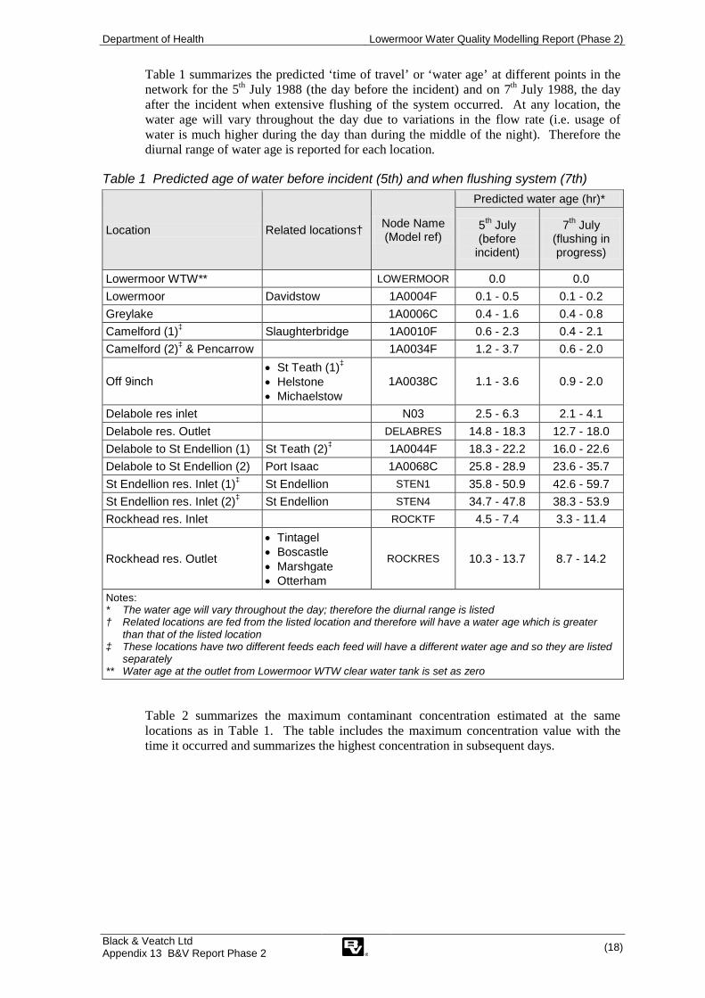
Table 1 summarizes the predicted ‘time of travel’ or ‘water age’ at different points in the network for the 5th July 1988 (the day before the incident) and on 7th
Table 1 Predicted age of water before incident (5th) and when flushing system (7th)
July 1988, the day after the incident when extensive flushing of the system occurred. At any location, the water age will vary throughout the day due to variations in the flow rate (i.e. usage of water is much higher during the day than during the middle of the night). Therefore the diurnal range of water age is reported for each location.
Location Related locations† Node Name (Model ref)
Predicted water age (hr)*
5th
(before incident)
July 7th
(flushing in progress)
July
Lowermoor WTW** LOWERMOOR 0.0 0.0 Lowermoor Davidstow 1A0004F 0.1 - 0.5 0.1 - 0.2 Greylake 1A0006C 0.4 - 1.6 0.4 - 0.8 Camelford (1) Slaughterbridge ‡ 1A0010F 0.6 - 2.3 0.4 - 2.1 Camelford (2)‡ & Pencarrow 1A0034F 1.2 - 3.7 0.6 - 2.0
Off 9inch • St Teath (1)• Helstone
‡
• Michaelstow 1A0038C 1.1 - 3.6 0.9 - 2.0
Delabole res inlet N03 2.5 - 6.3 2.1 - 4.1 Delabole res. Outlet DELABRES 14.8 - 18.3 12.7 - 18.0 Delabole to St Endellion (1) St Teath (2) 1A0044F ‡ 18.3 - 22.2 16.0 - 22.6 Delabole to St Endellion (2) Port Isaac 1A0068C 25.8 - 28.9 23.6 - 35.7 St Endellion res. Inlet (1) St Endellion ‡ STEN1 35.8 - 50.9 42.6 - 59.7 St Endellion res. Inlet (2) St Endellion ‡ STEN4 34.7 - 47.8 38.3 - 53.9 Rockhead res. Inlet ROCKTF 4.5 - 7.4 3.3 - 11.4
Rockhead res. Outlet
• Tintagel • Boscastle • Marshgate • Otterham
ROCKRES 10.3 - 13.7 8.7 - 14.2
Notes: * The water age will vary throughout the day; therefore the diurnal range is listed † Related locations are fed from the listed location and therefore will have a water age which is greater
than that of the listed location ‡ These locations have two different feeds each feed will have a different water age and so they are listed
separately ** Water age at the outlet from Lowermoor WTW clear water tank is set as zero
Table 2 summarizes the maximum contaminant concentration estimated at the same locations as in Table 1. The table includes the maximum concentration value with the time it occurred and summarizes the highest concentration in subsequent days.

Department of Health Lowermoor Water Quality Modelling Report (Phase 2)
Black & Veatch Ltd Appendix 13 B&V Report Phase 2 (19)
Table 2 Predicted maximum contaminant concentration
Location Related location Max concentration on day (mg/L Al) Time of
peak 6th 7th 8th 9th 10th 11th
Lowermoor WTW Davidstow 325 281 5 3 2 1 6th at 20:30 Lowermoor 325 281 5 3 2 1 6th at 20:30 Greylake 325 285 5 3 2 1 6th at 21:00 Camelford (1) Slaughterbridge 325 287 5 3 2 1 6th at 21:30 Camelford (2) & Pencarrow 325 303 5 3 2 1 6th at 22:15
Off 9inch • St Teath (1) • Helstone • Michaelstow
325 309 5 3 2 1 6th at 22:15
Delabole res inlet 323 324 5 3 2 1 7th at 00:00 Delabole res. Outlet 62 130 32 5 3 2 7th at 07:25 Delabole to St Endellion St Teath (2) 0 129 43 6 3 2 7th at 11:15 Delabole to St Endellion Port Isaac 0 123 78 9 5 2 7th at 16:45 St Endellion res. Inlet (1) St Endellion 0 0 123 24 4 2 8th at 06:15 St Endellion res. Inlet (2) St Endellion 0 0 129 18 2 2 8th at 02:45 Rockhead res. Inlet 238 322 5 3 2 1 7th at 03:45
Rockhead res. Outlet
• Tintagel • Boscastle • Marshgate • Otterham
67 193 21 4 2 1 7th at 12:00
3.3.1 Model representation of different locations
The model predictions listed in Table 1 and Table 2 above are for samples directly from the trunk main system (as shown in Figure 7). Before the contaminated water was received by consumers, it would have passed through local distribution pipes which have not been simulated. The implications of this for different locations are discussed below:
• Davidstow reservoir and supply area. This supply area consumes approximately 21% of the total supply from Lowermoor WTW (about 11 L/s on 5 July 1988). The area is represented by a demand node downstream of the Lowermoor clear water tank. The average age of water at Davidstow reservoir inlet is about 3.5 hours. However there are no other details available to assess the retention time in Davidstow reservoir or the age profile in the network downstream.
• Camelford. Camelford is supplied by two separate feeds from the trunk main network and is therefore represented by demand from two locations in the model. These feeds go direct into the town and so there would only be a short delay before Camelford residents could have received the contaminated water. However, within Camelford there is a local loop of pipe work feeding several dead end lengths. It is possible that contaminated water resided for extended periods in some of these deadends.
• Tintagel, Boscastle reservoir, Mashgate and Otterham. These areas are supplied from pipework downstream of Rockhead reservoir. The age of water and concentrations will reflect the results at the Rockhead reservoir outlet. The distribution system is complex downstream and any assessment would require the whole area to be modelled in detail. However results at the outlet will reflect the likely concentration profile as far as Boscastle reservoir. The concentration profile and age downsteam of Boscastle reservoir will relate directly to the retention time and hydraulic performance of the storage.
• Helstone and Michaelstow reservoir. These are supplied through a 6-inch main off the trunk main system near Camelford. There are no details available to assess the

Department of Health Lowermoor Water Quality Modelling Report (Phase 2)
Black & Veatch Ltd Appendix 13 B&V Report Phase 2 (20)
retention time in the storage, the effect of dilution within the tank or the age profile in the network downstream.
• St Teath. St Teath is supplied from two directions, one from the 6-inch main feeding Helstone and Michaelstow reservoir and the second off the mains between Delabole reservoir and St Endellion. Although the 4-inch connecting pipe is not modelled, the analysis results for the two modelled points either side of St Teath will reasonably represent the range of ages and concentrations at that location.
• Port Isaac. This town is supplied off the mains between Delabole reservoir and St Endellion. The local supply pipes are relatively short and therefore the trunk main model will reflect reasonably the ages and contaminant concentrations in the local pipework, albeit that peak concentrations and durations are likely to be delayed and extended by local hydraulic conditions.
• St Endellion. The results for St Endellion will reflect the conditions at the inlet to the St Endellion reservoir and any properties supplied upstream of the inlet. The hydraulics of the supply downstream are complicated by the following: - Mixing and retention time of the two sources within the reservoir; Lowermoor and
De Lank. This will be directly related to the relative proportions of the two supplies and the retention time/hydraulic conditions in the tank.
- Mixing and retention time within the reservoir of the contaminant with the stored water
- The timing of the use of the alternative water supply. It is known that the inlet from the Lowermoor system was shut at some time soon after the contamination was discovered and prior to the arrival of the contaminated water at the reservoir (ie the reservoir was fed only from the De Lank system), but that the valve was reopened at some later time when there was still aluminium sulphate in the Lowermoor system.
The implication of the above is that it is likely that concentrations of the contaminant within the stored water and entering the network downstream will be less that the predicted concentrations at the reservoir inlet.
4. INFLUENCE OF SLUDGE IN CONTACT TANK
There is conflicting information about whether there was a solid compacted deposit of sludge in the contact tank at the time of the incident (Reference 14). There is no documented information on the form or composition of this sludge, but if correct it would have a significant effect on the mixing within the contact tank and the concentration discharged into the clear water tank. We were therefore asked to:
1. Review the likelihood of such a sludge existing based on our technical knowledge of water treatment processes.
2. Repeat our modelling and analysis assuming that the contact tank was partially blocked by a compacted sludge.
The nature, consistency and profile of the sludge would each and collectively have had an impact. We have assumed that the sludge is a hard and fixed deposit so that the interface between the sludge and the water is equivalent to a rigid wall.
4.1 Sludge cause and characteristics
Raw waters containing turbidity and/or colour when treated with a coagulant (e.g. aluminium or iron salts) produce suspended solids made up of turbidity, colour solids and aluminium or ferric hydroxide depending on the coagulant used. When lime is used for coagulation pH correction the impurities in lime (about 4%) and some undissolved lime also contribute to the suspended solids.
Over 90% of suspended solids formed in the coagulation process and those contributed by lime are removed in clarifiers and a very high proportion of the remainder is removed in

Department of Health Lowermoor Water Quality Modelling Report (Phase 2)
Black & Veatch Ltd Appendix 13 B&V Report Phase 2 (21)
the filters. When lime is used for final pH correction the impurities in lime and undissolved lime usually settles in the contact tank or clear water tank depending on the location of the dosing point.
The current UK standard for turbidity of the final water is 1 NTU. The standard before 2001 was 4 NTU. The filtered water turbidity therefore should be less than these values as some allowance should be made for the contribution made by lime to turbidity.
The suspended solids removed in clarifiers are evacuated from the clarifiers regularly as sludge and solids removed in the filters are cleared from the filters by regular backwashing of the filters. The concentration of suspended solids in clarifier sludge may vary in the range 2.5 (for waters with colour) to 10 mg/l or more (for waters with high turbidity) and that in filter washwater is about 0.25 g/l irrespective of the raw water quality, provided the clarifier performance is satisfactory. The density and the nature of clarifier sludge is therefore a function of the raw water quality. If the water contains a high concentration of silt (similar to that found in tropical rivers) then clarifier sludge would be dense and silty, whereas if sludge is due to colour then sludge would be watery and gelatinous in nature.
4.1.1 Lowermoor sludge characteristics
In the case of Lowermoor the raw water contains moderate colour and low turbidity. Aluminium sulphate is used in the coagulation and lime is used for coagulation pH correction. Lime is also used in final pH correction and is dosed at the contact tank inlet.
The sludge produced in the clarifier would be gelatinous as it would be made up of colour solids and aluminium hydroxide. The contribution from lime and turbidity to the clarifier sludge would be small. The density of the sludge would be very similar to that of water. The washwater suspended solids would be very fine flocculant material and the density would also be very similar to that of water.
4.2 Likelihood of sludge in the contact tank
It is reported that sludge was observed in the contact tank at the outlet end up to the invert of the outlet pipe (which is at a high level) and it was of a consistency such that a person was able to stand on it. This is most unlikely because there would not be sufficient head room for a person to stand on top of the sludge (it is an enclosed tank). Also if sludge was up to the outlet level some sludge would have been carried into the clear water tank; no sludge was reported in the clear water tank. It is possible that the person was referring to the washout pipe which is normally located at the bottom of the contact tank and that he was standing on a thin layer of sludge lying on the floor of the tank.
The sludge if found in any structure downstream of the filters would be due to carryover of flocculant material from the filters and would be very fine material as it has to pass through a bed of fine sand in the filters. A small proportion of this material could settle in the contact tank and the clear water tank, but most of it would end up in the distribution system. The water quality data shows that the average filtered water turbidity was 0.5 NTU which is equal to about 1 mg/L suspended solids. This would give rise to about 6 kg/d of solids.
Also since final pH correction at the works takes the pH up to a value greater than 8.5 the aluminium hydroxide floc in the carry over from the filters would dissolve leaving only traces (much less than 6 kg/d) of inert material in the water entering the contact tank and the clear water tank. If it was allowed to accumulate, it would probably take many years to build up to the level of the outlet. Even then it would not be sufficiently dense for a person to stand on it.

Department of Health Lowermoor Water Quality Modelling Report (Phase 2)
Black & Veatch Ltd Appendix 13 B&V Report Phase 2 (22)
Any solids from lime used in the final pH correction, being heavy when compared to the turbidity carried over from the filters, would probably settle in the inlet end of the contact tank downstream of the dosing point. Assuming a maximum lime dose of 7 mg/L as 96% lime, the impurities and undissolved lime could contribute about 2 kg/d solids which would settle primarily at the inlet end of the contact tank. These solids if settled over several years in the contact tank would not form a surface sufficiently firm enough to allow a person to stand on it.
The use of lime could give rise to the formation of calcium carbonate precipitate due to ‘local softening’ at the point of application. This is a problem common to hard waters. Lowermoor water is soft and local softening would not normally take place.
In conclusion, based on a review by our treatment specialist:
• It is impossible that the contact tank contained sludge up to the outlet pipe invert and a person was able to stand on it.
• It is possible that the person mistook the washout pipe to the outlet pipe and he was standing on a thin layer of sludge laid on the floor of the tank as any sludge collected in the tank would not be firm enough for someone to stand on it.
4.3 Model of contact tank with sludge deposits
4.3.1 Assumed profile of sludge for model
The true profile of any compacted sludge is unknown, but the profile assumed in the model is as shown in Figure 20. The compacted sludge was reportedly to the depth of the outlet pipe. However, deep sludge deposits would not be possible where the flow passes through the holes in the wall because the holes are at low level. We have therefore assumed a constant grade of compacted sludge from zero depth immediately downstream of the holes to just below the invert of the outlet pipe at the outlet. In reality, you would not get a uniformly graded sludge as sediment would build up in regions of low velocity and be scoured away in regions of higher velocity. This would result in undulations in the sludge profile particularly at bends in the flow.
Figure 20 Assumed profile of compacted sludge
Section along Lane 1
Section along Lane 2
Lane 1
Lane 2
Lane 3
Brown indicates sludge

Department of Health Lowermoor Water Quality Modelling Report (Phase 2)
Black & Veatch Ltd Appendix 13 B&V Report Phase 2 (23)
4.3.2 Revised model setup
A similar modelling approach was used to the simulation without sludge in the contact tank.
1. Contact tank: A similar model setup was used with the following differences: - Model geometry: The geometry was changed to replicate the assumed profile for
the sludge (see Section 4.3.1) - Software: CFX version 5.10 - Mesh details: 325,000 elements. Although fewer elements compared to the
original model, the mesh was carefully setup so that the model accuracy should not be significantly impaired.
2. Clear water tank: Only the contact tank was assumed to contain sludge. The clear water tank was assumed to contain no sludge and so the model geometry remained unaltered. The previous model of the clear water tank was updated as follows: - The inlet boundary condition was updated with the concentration profile predicted
by the contact tank model with sludge present. - A more efficient mesh was built with 249,000 elements - Only a 12 hour period was simulated and the change in water level after 11 hours
was ignored. The peak concentration at the outlet occurs within 5 hours and over 75% of the aluminium has been discharged from the clear water tank after 12 hours. Therefore 12 hours simulation was considered sufficient for this model run.
3. Distribution network: The previous model of distribution network was updated with the revised concentration profile at the inlet from Lowermoor treatment works. Otherwise the model was unaltered from the previous simulation.
4.4 Model results with sludge present
4.4.1 Contact tank model predictions with sludge present
The predicted aluminium concentrations at various time intervals are shown in Figure 21. The ramped profile for the sludge has a significant influence on the predicted aluminium concentrations. There are two factors which appear to be counteractive on the concentration predicted at the outlet:
1. The raised bed level at the outlet lifts the stratified high concentration layer increasing the concentration at the outlet early on (before 1 hr).
2. The high concentration (dense) mixture tends to sink down the ramp formed by the sediment flowing against the principle direction of flow. This has the effect of trapping aluminium within the tank.
The combined affect of the above is that the predicted peak concentration at the outlet is higher and the alum persists in the tank for longer when the sludge is present. The predicted concentration profile for water exiting the contact tank is shown in Figure 22.

Department of Health Lowermoor Water Quality Modelling Report (Phase 2)
Black & Veatch Ltd Appendix 13 B&V Report Phase 2 (24)
Time Without Sludge With Sludge
10 min
30min
1hr
2hr
4hr
Figure 21 Predicted Al concentration in contact tank with and without sludge

Department of Health Lowermoor Water Quality Modelling Report (Phase 2)
Black & Veatch Ltd Appendix 13 B&V Report Phase 2 (25)
0
500
1000
1500
2000
2500
3000
0 1 2 3 4 5 6Time (hours)
Con
cent
ratio
n (m
g/L
Al)
0%
20%
40%
60%
80%
100%
% A
lum
Exp
elle
d Fr
om T
ank
Concentration without sludge Concentration with sludge% Alum expelled without sludge % Alum expelled with sludge
Time zero = start of discharge(approximately 17:00)
Figure 22 Predicted Al concentration at contact tank outlet with and without sludge
4.4.2 Clear water tank model predictions with sludge present in contact tank
The clear water tank model was rerun with the concentration profile at the inlet boundary replaced by the concentration profile predicted by the contact tank model with sludge present (as Figure 22). It was assumed that no sludge was present within the clear water tank and so the geometry of the model remained unaltered from the previous run.
The predicted aluminium concentrations in the clear water tank at various time intervals are shown in Figure 23. For the initial run (without sludge in the contact tank), the peak concentration entering the clear water tank was 1470 mg/L which would have a density of 1008 kg/m³. For the rerun (with sludge in the contact tank), the peak concentration entering the clear water tank was 2730 mg/L which would have a density of 1016 kg/m³. This increase in density makes the stratification in the clear water tank more severe, to the extent that although the peak concentration entering the tank is nearly double that of the initial run, the concentration towards the top of the tank remains lower than in the initial run.
The predicted concentration profiles exiting the clear water tank with and without sludge present in the contact tank are shown in Figure 24. These are the concentrations which would be entering the distribution system and therefore represent the maximum concentrations which according to these models could have been received by consumers. The peak concentration without sludge in the contact tank is 325 mg/L, whereas with sludge in the contact tank, the peak predicted concentration is 472 mg/L. It is worth noting that although the peak concentration entering the clear water tank has increased by 86% (1470 to 2730 mg/L), the peak concentration exiting the tank has only increased by 45% (325 to 472 mg/L). Hence, the clear water tank can be seen to have a buffering effect on the peak concentration entering the system.

Department of Health Lowermoor Water Quality Modelling Report (Phase 2)
Black & Veatch Ltd Appendix 13 B&V Report Phase 2 (26)
Time Without Sludge With Sludge
1hr
3hr
5hr
7hr
11hr
Figure 23 Predicted Al concentration in clear water tank with and without sludge

Department of Health Lowermoor Water Quality Modelling Report (Phase 2)
Black & Veatch Ltd Appendix 13 B&V Report Phase 2 (27)
0
100
200
300
400
500
0 5 10 15 20Time (hours)
Con
cent
ratio
n (m
g/L
Al)
0%
20%
40%
60%
80%
100%
% A
lum
Exp
elle
d Fr
om T
ank
Concentration with sludge Concentration without sludge% Alum expelled with sludge % Alum expelled without sludge
Time zero = start of discharge(approximately 17:00)
Figure 24 Predicted Al concentration at clear water tank outlet with and without sludge
4.4.3 Distribution network model predictions with sludge present in contact tank
The distribution network model was rerun with the concentration profile for the water supplied into the network from Lowermoor WTW replaced by the revised profile predicted by the CFD model of the clear water tank (Figure 24). No other changes were made to the network model. The maximum predicted concentrations within the network on successive days are shown in Table 3. The predicted concentrations are typically 45% higher than the equivalent predictions for no sludge present in the contact tank (Table 2), with the peak concentration arriving slightly earlier at each location.
The predicted concentration profiles for different locations within the network (with and without sludge present in the contact tank) are presented and discussed in Section 5.

Department of Health Lowermoor Water Quality Modelling Report (Phase 2)
Black & Veatch Ltd Appendix 13 B&V Report Phase 2 (28)
Table 3 Predicted maximum contaminant concentration with sludge in contact tank
Location Related location Max concentration on day (mg/L Al) Time of
peak 6th 7th 8th 9th 10th 11th
Lowermoor WTW Davidstow 472 357 0 0 0 0 6th at 19:15 Lowermoor 472 357 0 0 0 0 6th at 19:15 Greylake 472 380 0 0 0 0 6th at 19:45 Camelford (1) Slaughterbridge 471 382 0 0 0 0 6th at 20:15 Camelford (2) & Pencarrow 472 407 0 0 0 0 6th at 20:45
Off 9inch • St Teath (1) • Helstone • Michaelstow
472 415 0 0 0 0 6th at 22:15
Delabole res inlet 472 458 0 0 0 0 6th at 22:30 Delabole res. Outlet 108 187 31 2 0 0 7th at 05:45 Delabole to St Endellion St Teath (2) 0 187 43 2 0 0 7th at 11:00 Delabole to St Endellion Port Isaac 0 175 88 5 0 0 7th at 16:00 St Endellion res. Inlet (1) St Endellion 0 15 175 21 1 0 8th at 05:30 St Endellion res. Inlet (2) St Endellion 0 126 187 15 1 0 8th at 02:15 Rockhead res. Inlet 376 466 0 0 0 0 7th at 02:15
Rockhead res. Outlet
• Tintagel • Boscastle • Marshgate • Otterham
122 273 16 0 0 0 7th at 07:15
5. ANALYSIS AND DISCUSSION
5.1 Effect of Aluminium sulphate on pH in the Contact Tank
For given water characteristics and treatment process, it is possible to predict with reasonable accuracy the pH that would result from different concentrations of aluminium sulphate. Having derived this relationship, it is then possible to calculate the aluminium concentration which corresponds to pH measurements recorded by the on-line monitor at the inlet to the contact tank.
5.1.1 Characteristic water quality for Lowermoor WTW
Lowermoor raw water is coloured, very soft, low in hardness and alkalinity and slightly acidic. The water is treated with the coagulant aluminium sulphate to remove colour and particulate material and lime for pH adjustment to render the water non-aggressive to pipes and fittings etc.
Water quality data for the raw, settled and final waters at Lowermoor WTW has been reviewed for a few months either side of the incident in 1988. The typical range of the parameters which have an impact on pH value and the coagulation process are given in Table 4. This table is divided into three datasets:
• Dataset 1 (worst): A lower band of raw water quality at Lowermoor WTW • Dataset 2 (typical): The typical raw water quality at Lowermoor WTW • Dataset 3 (best): An upper band of raw water quality at Lowermoor WTW
Based on these three water quality datasets, we have used a water quality treatment model to calculate, the alum and lime doses required to treat the raw water. These calculated doses are also given in Table 4.

Department of Health Lowermoor Water Quality Modelling Report (Phase 2)
Black & Veatch Ltd Appendix 13 B&V Report Phase 2 (29)
Table 4 Typical Lowermoor WTW raw water quality in 1988 and calculated doses Parameter Dataset 1
(worst) Dataset 2 (typical)
Dataset 3 (best)
Typical raw water quality
pH value 5.2 6.0 6.7 Colour (Hazen) 62 50 25 Turbidity (NTU) 16 < 5 < 5 Total dissolved solid (mg/l) 60 75 90 Alkalinity (mg/l CaCO3 1 ) 3 6 Calcium (mg/l CaCO3 3 ) 3.5 4
Predicted doses
Alum dose mg/l8% Al2O 60 3 50 30 Lime dose mg/l as Ca(OH)2 14 to pH 6.0 9 3
The quantities of alum and lime used initially, and the raw water quality will have an impact on the subsequent effect of the alum discharged into the contact tank. The water quality data indicate that the ‘coagulation pH’ (the optimum pH for coagulation) is typically about 6.0.
From information provided the pH value of the water in the contact tank prior to the incident was approximately 9.8. The post lime doses required to obtain this value when starting from the coagulation pH of 6.0 would be 17, 8.5 or 7 mg/l respectively for the three conditions of water quality (calculated using the RTW model – Reference 15).
5.1.2 Alum dose and pH
The impact on pH value of the addition of alum in large quantities to each of the three treated waters is shown in Figure 25 (Reference 15).
2
3
4
5
6
7
8
9
10
0 5 10 15 20 25 30 35 40Alum (mg/L Al)
pH v
alue
Dataset 1 (worst)Dataset 2 (typical)Dataset 3 (best)
Assumed Water Quality set*
pH = 3.8
* Water quality datasets as defined in Table 4
Figure 25 pH versus Alum dose
It is reported that the pH value of water in the contact tank was approximately 3.8 after the incident, it can be seen from Figure 25 that the concentration of alum required to reach this value would be approximately 8 mg/L Al for dataset 1 (lower band) or 4 mg/L Al for datasets 2 and 3 (typical or upper band). Both models of the contact tank (with and without sludge present) predict concentrations in excess of 8 mg/L close to the inlet to the

Department of Health Lowermoor Water Quality Modelling Report (Phase 2)
Black & Veatch Ltd Appendix 13 B&V Report Phase 2 (30)
contact tank. It is not possible to give a direct comparison as the exact location of the pH meter in the contact tank at the time of the incident is unknown.
5.1.3 Note about pH measurements
pH is a measure of the hydrogen ion (H+) concentration (acidity) of a water and is recorded on a logarithmic scale on which 7.0 is neutral and 0 is equivalent to a Normal (N) strength solution, that is 1g/l of hydrogen ions. pH 1.0 is equivalent to a 0.1 N solution, pH 2.0 to a 0.01 N solution, pH 3.0 to a 0.001 N solution, etc. Thus for each decrease of one pH unit a ten fold increase in H+
Figure 25 ions is required, hence the initially steep drop in pH value
shown in , followed by a rapid ‘flattening out. For example, approximately one thousand times as much acid is required to ’achieve the pH change from 3.0 to 2.0 as is required for the change from 6 to 5.
It may also be noted that pH measurement is sometimes less reliable below about pH 4.5.
5.2 Comparison of sample data with model predictions
The following assessment is primarily based on the SWW distribution system sample data for pH, Al and S04 7 July to 4 August 1988 (Reference 7). The analysis is generally restricted to samples dated between 6th July and 11th
Limitations with the model results were set out in Section
July 1988, although data after that period has been reviewed where the local distribution network extends significantly beyond the modelled pipes. In addition to the SWW sample data, the assessment takes into account four private analyses of water samples (Reference 8). Unless stated otherwise all model results presented in this section relate to the simulations without sludge in the contact tank.
3.3. In particular it is important to recognise that the model predicts concentrations within the trunk mains whereas the SWW samples were taken from local distribution. The data sets are therefore not fully equivalent and some difference should be expected.
Figure 26 shows the predicted propagation of contaminant through the network. Further details for specific locations is given in Sections 5.2.1 to 5.2.7.

Department of Health Lowermoor Water Quality Modelling Report (Phase 2)
Black & Veatch Ltd Appendix 13 B&V Report Phase 2 (31)
0 hours (06/07/1988 17:00)
1.5 hours (06/07/1988 18:30)
3 hours (06/07/1988 20:00)
6 hours (06/07/1988 23:00)
12 hours (07/07/1988 05:00)
18 hours (07/07/1988 11:00)
24 hours (07/07/1988 17:00)
48 hours (08/07/1988 17:00)
72 hours (09/07/1988 17:00)
Figure 26 Predicted propagation of Al through trunk mains
< 1mg/L Al 1 - 10mg/L Al
10 - 100mg/L Al
> 100mg/L Al
N.B. These results apply to trunk mains only. Pockets of high concentration will have remained for considerably longer within distribution pipes.
Rockhead reservoir
Delabole reservoir
Lowermoor WTW

Department of Health Lowermoor Water Quality Modelling Report (Phase 2)
Black & Veatch Ltd Appendix 13 B&V Report Phase 2 (32)
5.2.1 Camelford
The model predictions for the Camelford area are shown in Figure 27 below. The first complaint was received at 19:55hrs on 6th
0
100
200
300
400
500
Wed 06 Jul 00:00 Thu 07 Jul 00:00 Fri 08 Jul 00:00 Sat 09 Jul 00:00 Sun 10 Jul 00:00 Mon 11 Jul 00:00
Con
cent
ratio
n (m
g/L
Al)
Camelford (1) Camel. (2) & Pencarrow SWW samples Private samples
Note :1. Dotted lines shows predictions for model runs with sludge in contact tank2. X Error bars are shown for samples without a recorded sample time3. Y Error bars indicates the range of results from repeat labortatory tests where done
Camel. 1
Camel. 2
Inci
dent
Sta
rtlin
e - 0
6 Ju
ly 1
7:00
July 1988. This is consistent with the model predicting the contaminant reaching Camelford at about 19:00hrs.
Figure 27 Predicted Al concentration on trunk mains in Camelford
Table 5 presents the SWW sample data for the Camelford area alongside the model predictions for the same date and time.
Table 5 Sample data for Camelford area
Date and Time Place Concentration (mg/L Al)
SWW Sample
Model Camel. (1)
Model Camel. (2)
07/07/88 10:55 Camelford 41.00 26 29 07/07/88 11:04 Slaughterbridge 50.00 25 28 08/07/88 12:00 Camelford 34.50 4 4 09/07/88 11:20 8 Roughtor Drive, Camelford 1.87 2 2 09/07/88 11:35 5 Longfield Road, Camelford 2.71 2 2 10/07/88 12:40 5 Longfield Drive, Camelford 1.07 1 2 10/07/88 12:55 8 Rough Tor Drive, Camelford 1.37 1 2
The bulk of the high aluminium concentration had passed the two supplies to Camelford by about midday on the 7th July. The sample, taken on 8th
A private sample taken on the night of 6
July, exhibits concentrations typical of the day before. This suggests that the sample could have been taken at a point not flushed on the previous day, possibly a dead end, at a consumers tap or from a consumer’s storage tank. Otherwise the model is consistent with the sample data.
th
One private sample was taken on the morning of 7
July was analysed by Berridge Environmental Laboratories Ltd and the Somerset County Analyst, Taunton in August 1988. The respective result of 188 mg/l and >0.5 mg/L are consistent with the modelled results.
th July and analysed by the Somerset County Analyst in December 1988. The measured aluminium concentration of 28 mg/L is consistent with the modelled results.

Department of Health Lowermoor Water Quality Modelling Report (Phase 2)
Black & Veatch Ltd Appendix 13 B&V Report Phase 2 (33)
A further sample taken on the 11th July was analysed by the Somerset County Analyst in August and December 1988. The sampling technique, location of sample point, the time the sample was taken, preceding hydraulic conditions time and hydraulic characteristics of the private pipe work can all impact on the sample. This sample was taken from the hot water tank filled on 7th
5.2.2 St Teath
July, where the contaminated water would have mixed with previously stored water. The respective results of >0.5 mg/L and 3.1 mg/L are consistent with the modelled results.
The model predictions for the St Teath area are shown in Figure 28 and Table 6 presents the SWW sample data for the St Teath area alongside the model predictions for the same date and time. St Teath can be supplied from two directions. The village of Pendogget is supplied off the trunk main between Delabole reservoir and St Endellion close to the take off for St Teath.
Figure 28 Predicted Al concentration on trunk mains in St Teath
Table 6 Sample data for St Teath area * Sample time unknown – model data for midday listed
Date and Time Place Concentration (mg/L Al)
SWW Sample
Model Off 9”
Model Del. to St E
08/07/88 10:50 St. Teath . 27.50 4 18 09/07/88 10:00 Pengavne, Pendogget 6.20 3 4 09/07/88 10:30 Bruallan Nursery, St. Teath 3.98 3 4 09/07/88 10:40 Vale View, Trewannan Lane, St. Teath 2.96 3 4 09/07/88 11:14 Bruallan Nursery, St. Teath 0.58 2 4
09/07/88 11:35 Vale View Bungalow Trewennan, St. Teath 0.97 2 4 10/07/88 10:50 Pengawne Bungalow, Pendoggett 0.96 2 2 11/07/88 * 2 Chapel Cane, Treveigan, St. Teath Hot Water 0.31 1 2 11/07/88 * 2 Chapel Cane, Treveigan, St. Teath Cold
Water 0.45 1 2

Department of Health Lowermoor Water Quality Modelling Report (Phase 2)
Black & Veatch Ltd Appendix 13 B&V Report Phase 2 (34)
One private sample taken at 05:00hrs on 7th July was analysed by Berridge Environmental Laboratories Ltd in August 1988, the Robens Institute at an unknown date and by the Somerset County Analyst in December 1988. The respective results of 460 mg/L, 720 mg/L and 620 mg/L are greater than the modelled results (both with and without sludge present in the contact tank). The model predicts that contaminated water would have entered the village from the south east after about 19:00hrs on 6th July, with the peak contamination of about 325 mg/L occurring after about 22:30 hrs that day. There is a second supply into the area, from the north west via the Delabole to St Endellion trunk main. The peak concentration from this main was about 130 mg/L and occurred at mid day on the 7th
5.2.3 Helstone and Michaelstow reservoir
July. It would appear that the private sample was taken from the former supply into St Teath.
The model predictions for the Helstone and Michaelstow reservoir area are shown in Figure 29 below.
Figure 27 Predicted Al concentration on trunk mains - Helstone and Michaelstow res.
Table 7 presents the SWW sample data for the area supplied from the trunk main at Helstone into the Michaelstow area and its service reservoir. The model results are consistent with the sample data.
Table 7 Sample data for Helstone and Michaelstow reservoir area
Date and Time Place Concentration (mg/L Al) SWW
Sample Model Off 9”
08/07/88 12:00 Michaelstow 4.39 4 09/07/88 12:06 5 Woodbine Cottage, Miehelston 0.81 2 09/07/88 13:55 Glebe View Bungalow, Michaelstow 0.98 2 09/07/88 14:10 Woodbine Cottage, Michaelstow 1.00 2

Department of Health Lowermoor Water Quality Modelling Report (Phase 2)
Black & Veatch Ltd Appendix 13 B&V Report Phase 2 (35)
5.2.4 Port Isaac and St Endellion
The model predictions for the Port Isaac and St Endellion reservoir areas are shown in Figure 30 below.
Figure 28 Predicted Al concentration on trunk mains in Port Isaac and St Endellion
Table 8 and Table 9 summarize the available sample data for Port Isaac and St Endellion respectively. The St Endellion system is complex and also supplied by a second source, De Lank water treatment works. The flow split between the two sources is not recorded and the bulk of the local distribution pipe work is not included in the hydraulic model. Accordingly the confidence in the model results for the St Endellion area is low. It is worth noting that no samples were taken in the St Endellion system between 8th and 11th
Overall, the model results for the Port Issac and St Endellion areas are consistent with the sample data.
July, the period when aluminium concentrations peaked.
Table 8 Sample data for Port Issac area * Sample time unknown – model data for midday listed
Date and Time Place Concentration (mg/L Al) SWW
Sample Model
Del. to St E. (2) 07/07/88 11:30 2 Mayfield Drive, Port Isaac (West) 9.00 7 08/07/88 10:40 26 St. Verse Road, Port Isaac 32.50 33 09/07/88 09:00 Trewetha Cottage, Trewetha. 6.93 5 09/07/88 09:10 Trewetha Farm, Trewetha. 7.70 5 09/07/88 09:30 Spar Shop, Port Isaac 10.08 5 09/07/88 * Port Isaac Fishemen Ltd 0.60 5 10/07/88 09:28 Trewetha Cottage, Nr. Port Isaac 1.00 2 10/07/88 09:45 Trewetha Farm, Trewetha, Nr. Port Isaac 0.80 2 10/07/88 10:00 The Spar Shop, Port Isaac 0.43 2 10/07/88 10:18 84 Fore Street, Port Isaac 0.60 2 11/07/88 11:30 Mayfield Drive, Port Isaac 0.69 2

Department of Health Lowermoor Water Quality Modelling Report (Phase 2)
Black & Veatch Ltd Appendix 13 B&V Report Phase 2 (36)
Table 9 Sample data for St Endellion area * Sample time unknown – model data for midday listed
Date and Time Place Concentration (mg/L Al) SWW
Sample Model
St E. res. inlet 07/07/88 11:00 Sycamoire Avenue Rock 0.10 0 07/07/88 * Blue Hills, Higher Triscon, Polzeath 0.06 0 07/07/88 * St. Endellion Service Reservoir 0.19 0
5.2.5 Delabole reservoir
The model predictions for the Delabole reservoir area are shown in Figure 31 below.
Figure 29 Predicted Al concentration on trunk mains in Delabole reservoir area
Table 10 summarizes the available sample data for the area supplied from Delabole reservoir. All samples were taken well after the peak concentrations as predicted by the model.
Table 10 Sample data for Delabole reservoir area
Date and Time Place Concentration (mg/L Al)
SWW Sample
Model Del. Inlet
Model Del. Outlet
08/07/88 11:20 Delabole Inlet 20.50 4 13 08/07/88 11:50 Delabole Outlet 2.26 4 13 09/07/88 11:00 34 Rock Road, Delabole 0.75 3 4 09/07/88 11:10 Rockmead Rock Road, Delabole 0.99 3 4 10/07/88 11:46 142 High Street, Delabole 0.47 2 2 10/07/88 12:02 33 Roch Head Road, Delabole 1.02 2 2 10/07/88 12:00 Rochead Rock Head Street, Delabole 1.00 2 2

Department of Health Lowermoor Water Quality Modelling Report (Phase 2)
Black & Veatch Ltd Appendix 13 B&V Report Phase 2 (37)
5.2.6 Area supplied from Rockhead reservoir
The model predictions for the Rockhead reservoir inlet and outlet are shown in Figure 32.
Figure 30 Predicted Al concentration on trunk mains in Rockhead reservoir area
Two SWW samples were taken on the inlet to Rockhead reservoir. These are compared against the equivalent model data in Table 11, however both samples were taken well after modelled peak and so the model predictions will have low confidence.
Table 11 Sample data for Rockhead reservoir inlet * Sample time unknown – model data for midday listed
Date and Time Place Concentration (mg/L Al) SWW
Sample Model
Rock. res. inlet 08/07/88 * Rockhead Inlet 21.00 4 08/07/88 * Rockhead Inlet 5.58 4
Table 12 summarises sample data for the area supplied from Rockhead reservoir including the Tintagel and Boscastle reservoir supply areas. There will have been a significant time lag between the water exiting Rockhead reservoir and the water entering the Boscastle supply area via Boscastle reservoir. Therefore, although the peak concentration passed through Rockhead reservoir about midday on 7th July, the peak will have occurred much later in the Boscastle supply area. Depending on the dilution effect and retention time in Boscastle reservoir, the peak could have been delayed until into 9th July 1988. Given this time lag, a direct comparison of modelled versus sample data is not very meaningful.

Department of Health Lowermoor Water Quality Modelling Report (Phase 2)
Black & Veatch Ltd Appendix 13 B&V Report Phase 2 (38)
Table 12 Sample data for Rockhead reservoir supply area * Sample time unknown – model data for midday listed
Date and Time Place Concentration (mg/L Al) SWW
Sample Model
Rock. res. outlet 07/07/88 12:46 Bocastle Service Reservoir 109.00 165 07/07/88 12:51 Bocastle Service Reservoir 7.90 165 07/07/88 13:49 Rockhead Service Reservoir 32.00 136 08/07/88 * Bocastle Inlet 2.17 6 09/07/88 09:30 Vine Cottage, Boscastle 5.29 3 09/07/88 11:04 Hillside Cottage, High Street, Boscastle 1.95 3 09/07/88 11:16 Cottage High Street, Boscastle 1.93 3 09/07/88 11:25 Hillside Bocastle Hot Water 0.23 3 09/07/88 11:40 Polkerr, Tintagel 0.49 3 09/07/88 11:51 Vine Cottage, Boscastle 0.82 3 09/07/88 11:53 Orchard House, Boscastle Cold Water 1.68 3 09/07/88 12:04 Fairfield Fore Street, Boscastle Cold Water 0.90 3 09/07/88 12:25 Hillside Bocastle Cold Water 0.90 3 09/07/88 12:43 Grange Cottage Bossiney 0.80 3 09/07/88 12:56 Tintagel Cold Water 0.39 3 10/07/88 11:00 Orchard House, Boscastle 0.46 2 10/07/88 11:49 Heigh-Ho Boscastle Hillside 0.61 2 10/07/88 12:02 Vine Cottage, Boscastle Hot Water 0.33 2 10/07/88 12:20 Orchard House, Boscastle Hot Water 0.18 2 10/07/88 12:41 Fairfield Fore Street, Boscastle Hot Water 0.58 2 10/07/88 12:54 Grange Cottage, Bossinor 0.91 2 11/07/88 13:30 Grange Cottage, Bossiney Hot Water 1.32 1 11/07/88 14:00 Tintagel Hot Water 0.68 1
5.2.7 Area supplied from Davidstow reservoir
The model predictions for the Davidstow reservoir area are shown in Figure 33 below
Figure 31 Predicted Al concentration on trunk mains in Davidstow reservoir area
Table 13 summarizes the available sample data for the area supplied from Davidstow reservoir, which is assumed to include the Marshgate and Otterham supply area.

Department of Health Lowermoor Water Quality Modelling Report (Phase 2)
Black & Veatch Ltd Appendix 13 B&V Report Phase 2 (39)
Table 13 Sample data for Davidstow reservoir area * Sample time unknown – model data for midday listed
Date and Time Place Concentration (mg/L Al) SWW
Sample Model
Del. to St E. (2) 08/07/88 * Davidstow Inlet . 1.80 4 08/07/88 * Davidstow Outlet 6.00 4 09/07/88 08:54 Treven "A" Marshgate Hot Water 4.86 3 09/07/88 09:09 Treven, Marshgate 11.97 3 09/07/88 10:17 ESSO Garage, Otterham Station 10.26 2 09/07/88 10:32 2 Westwinds, Otterham Station Hot Water 0.07 2
All the samples were taken well after the model predicts the peak to have passed and so the model predictions will be unreliable. In addition to this:
• The time of travel to and dilution and retention time in the Davidstow reservoir can not been modelled. However the peak concentration will have occurred at least 3 hours later than the model predicts the peak at Lowermoor water treatment works.
• The extent of the distribution pipework downstream of Davidstow reservoir and the demand in the area are unknown, both of which could have a significant impact on the concentration at a particular point in the network at a particular time.
• It is possible that both Marshgate and Otterham were supplied from Boscastle, not via Davidstow as assumed here. If so the peak concentration would have arrived considerably latter (possibly a day or more latter). This could explain the apparently elevated concentrations recorded at Marshgate and Otterham on the 9th
• The age of the water of samples taken from a hot water system is unknown. Therefore two of the samples are likely to be for water delivered earlier than the sampling date.
July.
5.3 Model accuracy
5.3.1 CFD models
Any modelling method will have sources of error and uncertainty. For CFD these can be divided into three main categories:
1. Model (theory) errors: These errors are caused where the theory assumed by the model does not exactly replicate the real behaviour. We believe that these errors will be small in this case as the conditions being modelled are not highly stressed and similar to those for which CFD simulations have been validated.
2. Calculation errors: The accuracy of the solution is determined by the level of convergence of the iterative calculations. The accuracy is also influenced by the detail of the mesh (discretisation); the finer the mesh, the more accurately the model can resolve behaviour. We believe that in this case these errors will be small for the following reasons: - We have used industry leading software (Ansys CFX 5.7 / 5.10) - The mesh detail is relatively high and well above the recommendations given in
the AwwaRF publication “Water quality modelling of Distribution System Storage Facilities”
- All models converged well (<10-4
3. Application uncertainties: These are errors caused because the setup of the model does not truly represent the actual conditions being simulated. This will be the most significant cause of error in this case. In particular the following uncertainties in the model setup could affect the accuracy of model predictions:
RMS)
- Inaccuracies in the information used to setup the models would cause inaccuracies in the model predictions (see Section 2.1)

Department of Health Lowermoor Water Quality Modelling Report (Phase 2)
Black & Veatch Ltd Appendix 13 B&V Report Phase 2 (40)
- There is some uncertainty over the model coefficients associated with the diffusivity of aluminium sulphate. If alternative values were used then the predicted rate of mixing could be increased. However, if the rate of mixing was significantly higher then the aluminium sulphate would not have been predicted to migrate upstream along the base against the main flow stream. The fact that it did migrate upstream is validated by the triggering of the pH alarm at the inlet to the tank.
- The geometry of the tank has been assumed to be exactly as shown on the drawings used to build the model. If the tank was modified between the date of these drawings and the date of the incident then these changes will not be included by the model.
- As discussed in Section 4 there has been some speculation about solid sludge deposits blocking the contact tank. If so this would reduce the accuracy of the model significantly.
Overall, we have reasonable confidence in the accuracy of the CFD models. Nevertheless, in order to determine a maximum theoretical limit for the aluminium exiting the contact tank, two spreadsheet calculations have been performed:
• Fully mixed in last section of contact tank: This represents an upper limit for a fully mixed solution, but is unrealistic because it does not replicate the migration of the aluminium sulphate back towards the contact tank inlet as confirmed by the pH probe at the inlet. This calculation predicts a maximum aluminium concentration of 4800 mg/L Al exiting the tank with there still being a trace concentration in the tank after 3.5 hours (20:30).
• Direct injection into outlet pipe: i.e. dilution proportional to outlet flow only. This is also not realistic because it is known that the pollutant injection point was at the upstream end of the last leg and not at the outlet. This calculation predicts a peak concentration of 5660 mg/L Al exiting the contact tank with it being clear within minutes of the completion of the tanker discharge.
Figure 34 presents the concentration curves for the CFD analysis and the comparative spreadsheet calculations. This figure defines the extremes for the range of aluminium concentration at the contact tank outlet and entering the clear water tank.
0
1000
2000
3000
4000
5000
6000
0.0 1.0 2.0 3.0 4.0Time (hours)
Con
cent
ratio
n (m
g/L
Al)
CFD Model without sludge CFD Model with sludgeFully mixed final section model Direct injection into outlet model
Time zero = start of discharge (approxcimately 17:00)
Figure 32 Comparison of CFD prediction with simple spreadsheet models
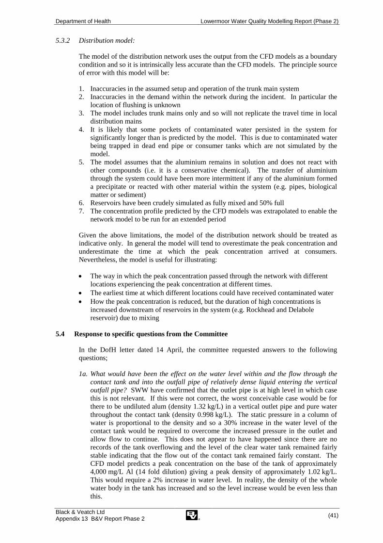
Department of Health Lowermoor Water Quality Modelling Report (Phase 2)
Black & Veatch Ltd Appendix 13 B&V Report Phase 2 (41)
5.3.2 Distribution model:
The model of the distribution network uses the output from the CFD models as a boundary condition and so it is intrinsically less accurate than the CFD models. The principle source of error with this model will be:
1. Inaccuracies in the assumed setup and operation of the trunk main system 2. Inaccuracies in the demand within the network during the incident. In particular the
location of flushing is unknown 3. The model includes trunk mains only and so will not replicate the travel time in local
distribution mains 4. It is likely that some pockets of contaminated water persisted in the system for
significantly longer than is predicted by the model. This is due to contaminated water being trapped in dead end pipe or consumer tanks which are not simulated by the model.
5. The model assumes that the aluminium remains in solution and does not react with other compounds (i.e. it is a conservative chemical). The transfer of aluminium through the system could have been more intermittent if any of the aluminium formed a precipitate or reacted with other material within the system (e.g. pipes, biological matter or sediment)
6. Reservoirs have been crudely simulated as fully mixed and 50% full 7. The concentration profile predicted by the CFD models was extrapolated to enable the
network model to be run for an extended period
Given the above limitations, the model of the distribution network should be treated as indicative only. In general the model will tend to overestimate the peak concentration and underestimate the time at which the peak concentration arrived at consumers. Nevertheless, the model is useful for illustrating:
• The way in which the peak concentration passed through the network with different locations experiencing the peak concentration at different times.
• The earliest time at which different locations could have received contaminated water • How the peak concentration is reduced, but the duration of high concentrations is
increased downstream of reservoirs in the system (e.g. Rockhead and Delabole reservoir) due to mixing
5.4 Response to specific questions from the Committee
In the DofH letter dated 14 April, the committee requested answers to the following questions;
1a. What would have been the effect on the water level within and the flow through the contact tank and into the outfall pipe of relatively dense liquid entering the vertical outfall pipe? SWW have confirmed that the outlet pipe is at high level in which case this is not relevant. If this were not correct, the worst conceivable case would be for there to be undiluted alum (density 1.32 kg/L) in a vertical outlet pipe and pure water throughout the contact tank (density 0.998 kg/L). The static pressure in a column of water is proportional to the density and so a 30% increase in the water level of the contact tank would be required to overcome the increased pressure in the outlet and allow flow to continue. This does not appear to have happened since there are no records of the tank overflowing and the level of the clear water tank remained fairly stable indicating that the flow out of the contact tank remained fairly constant. The CFD model predicts a peak concentration on the base of the tank of approximately 4,000 mg/L Al (14 fold dilution) giving a peak density of approximately 1.02 kg/L. This would require a 2% increase in water level. In reality, the density of the whole water body in the tank has increased and so the level increase would be even less than this.

Department of Health Lowermoor Water Quality Modelling Report (Phase 2)
Black & Veatch Ltd Appendix 13 B&V Report Phase 2 (42)
1b. If the outfall was delayed because of the higher density of water in the vertical pipe how soon would normal flows have resumed once the greater part of the high density liquid has passed through the outfall pipe? Not relevant. See answer to 1a above. However it is worth noting that in a gravity system any forced or uncontrolled change to the hydraulic gradient will be compensated for relatively quickly within the flow and level control points, with overflow discharges taking place if necessary. There are no reports of overflows occurring within the works or at either of the tanks on the site, although both tanks include overflow structures.
2. What concentration of aluminium is likely to have been present in the outflow from the outlet pipe over the time period needed to have extracted most of the contaminated water from the contact tank? See the curves for the individual tanks (Figure 15 and Figure 19).
3. What would have been the likely effect of dilution on this outflow in the small basin in the treated water tank upstream of the weir that contained the outlet pipe from the contact tank? SWW has confirmed that there is no inlet weir on the inlet pipe to the clear water tank. The top of the pipe comprises a bellmouth as shown on the original reservoir drawing (Reference 01).
4. If the solution in this small basin is relatively concentrated how would the denser liquid overflowing from the chamber into the main treated water tank have behaved in its passage through the treated water tank? Would there still have been plug flow through the treated water tank or would a sheet flow across the base of the treated water tank to its final outlet have been possible? In either case what would have been the estimated concentration of the outlet of the treated water tank and over what period? As stated in 3 above there is no separate inlet chamber. The plots of the performance of the tank illustrate the short circuiting in the tank combined with the stratification by concentration. Note also that the bottom water level outlet mitigates the effect of stratification.
5. The likelihood of compacted sludge in the base on the contact tank. From our experience and knowledge of the water chemistry of the Lowermoor source, our treatment works specialist does not believe that the “sediment” reported to have settled in the floor of the contact tank would have been hard (see Section 4 for a full discussion).
6. Distribution system dead ends. Dead ends and through pipes with very low flows may happen to draw off a large slug of contaminated water due to a localized short term period of high demand. Once the dead end had been “filled” with water of a particular concentration, it would remain in the section of pipe until it had been used or leaked away. There would however be a dilution effect from lower concentration water “topping up” the dead end as water is used, but again the rate of dilution will depend on the local demand patterns. However once fully mixed, the concentration of the contaminant will not increase due to extended retention in a pipe or storage.
7. Elevation of pipes. The elevation of the pipe will have no effect on the pollution levels.
8. Plug flow and flushing. The distribution network is a “closed” (or pressurized) pipe system operating effectively as plug flow with dispersion taking place at leading and trailing edges. Demands from the system, be they domestic, commercial, or a flushing exercise do not alter the basic hydraulics of closed pipe systems. Even when the system is being flushed it is still a closed system. There has been no mention of the network being drained down completely and then refilled, a condition which would be more akin to being analysed as a sewer, e.g. open channel.

Department of Health Lowermoor Water Quality Modelling Report (Phase 2)
Black & Veatch Ltd Appendix 13 B&V Report Phase 2 (43)
6. CONCLUSIONS
1. Computer modelling has been used to simulate the discharge of aluminium sulphate at Lowermoor WTW and the resultant propagation of aluminium through the trunk main system which supplies Camelford and surrounding areas. The methodology used in this study was to analyse each component of the system in turn using the output of the upstream component as the input for the next component: - Model of contact tank - Model of clear water tank - Model of distribution network (trunk mains only) The two tanks were analysed using CFD software which simulated the three dimensional hydraulics and dispersion of aluminium sulphate. The distribution model is one dimensional and does not simulate dispersion or buoyancy affects. All three models assume that the aluminium remains in solution and does not react with other compounds (i.e. it is a conservative chemical).
2. The CFD modelling supports the belief that the aluminium sulphate sank to the bottom of the contact tank and migrated throughout the floor of the tank. This is validated by the pH meter readings which indicated that the pH increased near the inlet, probably due to the presence of aluminium sulphate which had migrated upstream against the main flow in the tank.
3. The sample data indicates that low level contamination concentrations persisted for at least a month after the incident. This is consistent with the model conclusions for the decay curve for the aluminium sulphate out of the Lowermoor clear water tank, the subsequent retention in service reservoirs and the distribution system downstream.
4. The models of the tanks only cover the first 24 hour period, beyond this time, water company sample data will be a more reliable indication of concentrations than the models.
5. A concentration against time profile has been predicted for the water exiting the clear water tank (Figure 19). The implications for this in the network have also been modelled at trunk main level only. The peak values predicted within the network are given in Table 2. The values are reasonably consistent with the majority of the SWW sample data.
6. One private sample is anomalous with the modelling results. This is the sample from Mayrose Farm St Teath taken on 7th July 1988 (analysed December 1988). We are unable to explain this anomaly.
7. We have re-run the analysis to simulate the effect of a large volume of hard compacted sludge in the contact tank. This simulation assumed that the compacted sludge formed a ramp up to just below the invert of the outlet pipe as shown in Figure 20. The models predicted that the presence of this sludge would cause the peak concentration exiting the contact tank to increase by 86% (from 1470 to 2730 mg/L). However, the clear water tank has a buffering effect so that the peak concentration predicted entering the distribution system increases by only 45% (325 to 472 mg/L).
8. We have reviewed the potential causes of sludge and how the likelihood of the formation of extensive deposits of a hard compacted sludge in the contact tank at Lowermoor WTW. Our review takes into account the treatment processes and water chemistry at the time of the incident and is independent of the output of the models presented in this report. It is the opinion of our water treatment specialist that it is impossible for the contact tank to have contained sludge up to the outlet pipe invert and that a person was able to stand on it. However, it is possible that the washout pipe (at low level) was mistaken for the outlet pipe and that there was a thin layer of sludge laid on floor close by.

Department of Health Lowermoor Water Quality Modelling Report (Phase 2)
Black & Veatch Ltd Appendix 13 B&V Report Phase 2 (44)
REFERENCES AND INFORMATION SOURCES
1. Lowermoor reservoir, General Details, April 1971
2. Drawing 16/805/A – Conversion of ex. Reservoir to Contact Tank, June 1972
3. 1:25,000 map showing DMAs (returned to DH )
4. A4 Copy of Item 3
5. Lowermoor Raw Water Flow Chart, 4th – 11th July 1988
6. Lowermoor Clear Water Tank Water Level Chart, 4th – 11th July 1988
7. SWW Distribution System Sample data for pH, Al and S04 7/7 to 4/8 1988
8. Private Samples Analysis data for samples taken 6 – 11 July 1988
9. Crowther Clayton Report dated 12 June 2003
10. Crowther Clayton Report dated 21 November 2003
11. Crowther Clayton Report dated 11 December 1993
12. Works schematics – Fax dated 27/03/02
13. SWW spine main model and report 1993 (from B&V archive)
14. COT Lowermoor Subgroup, Consultation Report, Paragraph 3.19, January 2005
15. Rothberg, Tamburini and Winsor (RTW) model, American Water Works Associtation