Embed Size (px)
Citation preview

FINAL REPORT (18/09/12)
Southern Cross GeoScience Report 112 Prepared for the South Australian Department of
Environment, Water and Natural Resources (DEWNR)
Lower Lakes Phase 1 Sulfate Reduction Monitoring Project

Lower Lakes Phase 1 Sulfate Reduction Monitoring Project Authors L.A. Sullivan, N.J. Ward, R.T. Bush, M.D. Cheetham, P.J. Cheeseman, D.M. Fyfe, T. McIntyre, M. Bush and R. Hagan Centre for Acid Sulfate Soil Research Southern Cross GeoScience Southern Cross University PO Box 157 Lismore NSW 2480 Permissive licence © State of South Australia through the Department of Environment, Water and Natural Resources and Southern Cross GeoScience. Apart from fair dealings and other uses permitted by the Copyright Act 1968 (Cth), no part of this publication may be reproduced, published, communicated, transmitted, modified or commercialised without the prior written approval of the Department of Environment, Water and Natural Resources and Southern Cross GeoScience. Written requests for permission should be addressed to: Coorong, Lower Lakes and Murray Mouth Program Department of Environment, Water and Natural Resources GPO Box 1047 Adelaide SA 5001 and: Centre for Acid Sulfate Soil Research Southern Cross GeoScience Southern Cross University GPO Box 157 Lismore NSW 2480 Disclaimer This report has been prepared by consultants for the Department of Environment, Water and Natural Resources (DEWNR) and views expressed do not necessarily reflect those of the DEWNR. The DEWNR cannot guarantee the accuracy of the report, and does not accept liability for any loss or damage incurred as a result of relying on its accuracy. Printed on recycled paper September 2012 ISBN ###-#-######-##-# Citation This report should be cited as:
Sullivan, L.A., Ward, N.J., Bush, R.T., Cheetham, M.D., Cheeseman, P.J., Fyfe, D.M., McIntyre, T., Bush, M. and Hagan, R. (2012) Lower Lakes Phase 1 Sulfate Reduction Monitoring Project. Southern Cross GeoScience Technical Report No. 112. Prepared for the SA Department of Environment, Water and Natural Resources, Adelaide.
Southern Cross University Disclaimer Southern Cross University advises that the information contained in this publication comprises general statements based on scientific research. The reader is advised and needs to be aware that such information may be incomplete or unable to be used in any specific situation. No reliance or actions must therefore be made on that information without seeking prior expert professional, scientific and technical advice. To the extent permitted by law, Southern Cross University (including its employees and consultants) excludes all liability to any person for any consequences, including but not limited to all losses, damages, costs, expenses and any other compensation, arising directly or indirectly from using this publication (in part or in whole) and any information or material contained in it. Authors: Prof. L.A. Sullivan, Dr N.J. Ward, Prof. R.T. Bush, Dr M.D. Cheetham, Mr P.J.
Cheeseman, Ms D.M. Fyfe, Mr T. McIntyre, Ms M. Bush and Ms R. Hagan. Reviewers: Approved by: Prof. L.A. Sullivan
Signed: Date: 18th September, 2012 Distribution: SA Department of Environment, Water and Natural Resources, Southern Cross
GeoScience Circulation: Public Domain

Lower Lakes Phase 1 Sulfate Reduction Monitoring Project
Page i
Contents LIST OF FIGURES............................................................................................................................................... III
LIST OF TABLES ................................................................................................................................................ IX
LIST OF ABREVIATIONS.................................................................................................................................... X
EXECUTIVE SUMMARY.................................................................................................................................... XI
1.0 PROJECT OVERVIEW ..............................................................................................................................1
2.0 AIM .........................................................................................................................................................1
3.0 INTRODUCTION ......................................................................................................................................2
3.1 BACKGROUND ON ACID SULFATE SOILS..............................................................................................................2 3.1.1. General ........................................................................................................................................... 2 3.1.2 Characteristics and formation ...................................................................................................... 2 3.1.3 Occurrence ..................................................................................................................................... 3 3.1.4 Analysis ............................................................................................................................................. 3 3.1.5 Minerals and reductive processes ................................................................................................ 3 3.1.6 Minerals and oxidation processes................................................................................................. 5 3.1.7 Pyrite oxidation................................................................................................................................ 6 3.1.8 Hazards from acid sulfate soils....................................................................................................... 6 3.1.9 Inundation of acid sulfate soils .................................................................................................... 11
3.2 INTRODUCTION TO THIS STUDY ..........................................................................................................................11 3.3 SAMPLING STRATEGY.......................................................................................................................................12 3.4 LOWER LAKES SITE LOCATIONS AND CHARACTERISTICS......................................................................................14
3.4.1 Waltowa, east Lake Albert study area characteristics ............................................................ 14 3.4.2 Poltalloch, east Lake Alexandrina study area characteristics ................................................ 16 3.4.3 Tolderol, west Lake Alexandrina study area characteristics ................................................... 17 3.4.4 Campbell Park, west Lake Albert study area characteristics ................................................. 20
4.0 MATERIALS AND METHODS..................................................................................................................21
4.1 FIELD SAMPLING OF SOILS ................................................................................................................................21 4.2 LABORATORY ANALYSIS METHODS....................................................................................................................23
4.2.1 General comments....................................................................................................................... 23 4.2.2 Sediment analyses ........................................................................................................................ 23 4.2.3 Sulfate reduction analyses........................................................................................................... 24 4.2.4 Pore-water analyses ..................................................................................................................... 25 4.2.5 Expression of results ....................................................................................................................... 25 4.2.6 Quality assurance and quality control ....................................................................................... 25
5.0 RESULTS .................................................................................................................................................27
5.1 GENERAL SEDIMENT CONDITION ......................................................................................................................27 5.1.1 Waltowa......................................................................................................................................... 27 5.1.2 Poltalloch ....................................................................................................................................... 38 5.1.3 Tolderol ........................................................................................................................................... 42 5.1.4 Campbell Park............................................................................................................................... 49
5.2 PORE-WATER PROPERTIES ................................................................................................................................56 5.2.1 Waltowa......................................................................................................................................... 56 5.2.2 Poltalloch ....................................................................................................................................... 61 5.2.3 Tolderol ........................................................................................................................................... 63 5.2.4 Campbell Park............................................................................................................................... 66
5.3 SULFATE REDUCTION RATES ..............................................................................................................................69 5.3.1 Waltowa sulfate reduction rates................................................................................................. 69 5.3.2 Sulfate reduction rates at Poltalloch .......................................................................................... 73 5.3.3 Sulfate reduction rates at Tolderol.............................................................................................. 75 5.3.4 Sulfate reduction rates at Campbell Park ................................................................................. 77
5.4 DISCUSSION....................................................................................................................................................79 5.4.1 Remediation of acidified sediment layers ................................................................................. 79 5.4.2 The nature of sulfur cycling and organic matter decomposition during the initial inundation of the Lower Lakes sediments........................................................................................... 80 5.4.3 Metal and metalloid dynamics in the sediments resulting from bioremediation ................. 82 5.4.4 Nutrient dynamics in the sediments resulting from bioremediation ....................................... 83
6.0 CONCLUSIONS.....................................................................................................................................85

Lower Lakes Phase 1 Sulfate Reduction Monitoring Project
Page ii
7.0 RECOMMENDATIONS...........................................................................................................................86
8.0 REFERENCES..........................................................................................................................................88
9.0 APPENDICES .........................................................................................................................................96
APPENDIX 1. SITE AND SAMPLE DESCRIPTIONS......................................................................................................97 APPENDIX 2. CHARACTERISTICS OF SOIL MATERIALS ...........................................................................................102 APPENDIX 3. DATA FOR SULFATE REDUCTION RATE SAMPLES ...............................................................................113 APPENDIX 4. PORE-WATER CHARACTERISTICS....................................................................................................124 APPENDIX 5. PORE-WATER PLOTS......................................................................................................................134 APPENDIX 6. HCL EXTRACTABLE METAL PLOTS ...................................................................................................157 APPENDIX 7. ADDITIONAL INFORMATION ..........................................................................................................174

Lower Lakes Phase 1 Sulfate Reduction Monitoring Project
Page iii
List of Figures Figure 3-1. Map showing study areas in the Lower Lakes (Source: Google Maps)...................................13 Figure 3-2. Waltowa sampling locations (Source: Google Maps)................................................................14 Figure 3-3. Sediment cores collected from the Phragmites site (left)..........................................................15 Figure 3-4. Sediment cores collected from the Juncus site at Waltowa in March 2012. .........................15 Figure 3-5. Comparison of the sediment cores collected from the Phragmites site (left core) ..............15 Figure 3-6. Poltalloch sampling locations (Source: Google Maps). .............................................................16 Figure 3-7. Tolderol sampling locations (Source: Google Maps)..................................................................17 Figure 3-8. Sampling at Tolderol in March 2012...............................................................................................17 Figure 3-9. Sediment core collected from the scald site (left) and iron segregation (right) at Tolderol in
March 2012. ................................................................................................................................................18 Figure 3-10. Iron segregations (left) and iron/jarosite (right) in the sediment core ...................................18 Figure 3-11. Sediment cores collected from the vegetated (Juncus in Bevy rye) site at Tolderol in
March 2012. ................................................................................................................................................18 Figure 3-12. Comparison of the sediment cores collected from the vegetated (left core) and scald
(right core) sites. .........................................................................................................................................19 Figure 3-13. Campbell Park sampling locations (Source: Google Maps). ..................................................20 Figure 4-1. Sediment sampling at Tolderol (March 2012)...............................................................................22 Figure 5-1. Waltowa field pH dynamics at the established Phragmites site (August 2010, February 2011
and March 2012)........................................................................................................................................27 Figure 5-2. Waltowa field pH dynamics at the established Cotula site (August 2010, February 2011 and
March 2012). ...............................................................................................................................................28 Figure 5-3. Waltowa field pH dynamics at the established Juncus site (August 2010, February 2011
and March 2012)........................................................................................................................................28 Figure 5-4. Waltowa TAA dynamics at the established Phragmites site (May 2010 – March 2012)........29 Figure 5-5. Waltowa TAA dynamics at the established Cotula site (May 2010 – March 2012). ..............29 Figure 5-6. Waltowa TAA dynamics at the established Juncus site (May 2010 – March 2012). ..............29 Figure 5-7. Waltowa field Eh dynamics at the established Phragmites site (May 2010 – March 2012)..30 Figure 5-8. Waltowa field Eh dynamics at the established Cotula site (May 2010 – March 2012). ........30 Figure 5-9. Waltowa field Eh dynamics at the established Juncus site (May 2010 – March 2012). ........31 Figure 5-10. Waltowa EC dynamics at the established Phragmites site (May 2010 – March 2012)........31 Figure 5-11. Waltowa EC dynamics at the established Cotula site (May 2010 – March 2012). ..............32 Figure 5-12. Waltowa EC dynamics at the established Juncus site (May 2010 – March 2012). ..............32 Figure 5-13. Waltowa pyritic sulfur dynamics at the established Phragmites site (May 2010 – March
2012). ............................................................................................................................................................33 Figure 5-14. Waltowa pyritic sulfur dynamics at the established Cotula site (May 2010 – March 2012).
.......................................................................................................................................................................33 Figure 5-15. Waltowa pyritic sulfur dynamics at the established Juncus site (May 2010 – March 2012).
.......................................................................................................................................................................33 Figure 5-16. Waltowa AVS dynamics at the established Phragmites site (May 2010 – March 2012). ....34 Figure 5-17. Waltowa AVS dynamics at the established Cotula site (May 2010 – March 2012). ............34 Figure 5-18. Waltowa AVS dynamics at the established Juncus site (May 2010 – March 2012). ............34 Figure 5-19. Elemental sulfur characteristics at the Waltowa study area (March 2012). .........................35 Figure 5-20. Waltowa TOC at Phragmites site (August 2010, February 2011 and March 2012). .............35 Figure 5-21. Waltowa hydrolysable C at Phragmites site (August 2010, February 2011 and March
2012). ............................................................................................................................................................36 Figure 5-22. Waltowa TOC at Cotula site (August 2010, February 2011 and March 2012). .....................36 Figure 5-23. Waltowa hydrolysable C at Cotula site (August 2010, February 2011 and March 2012). ..36 Figure 5-24. Waltowa TOC at Juncus site (August 2010, February 2011 and March 2012). .....................37 Figure 5-25. Waltowa hydrolysable C at Juncus site (August 2010, February 2011 and March 2012). ..37 Figure 5-26. Poltalloch field pH dynamics at the Bevy rye site (August 2010, February 2011 and March
2012). ............................................................................................................................................................38 Figure 5-27. Poltalloch TAA dynamics at the Bevy rye site (May 2010 – March 2012). .............................38 Figure 5-28. Poltalloch field Eh dynamics at the Bevy rye site (May 2010 – March 2012). .......................39 Figure 5-29. Poltalloch EC dynamics at the Bevy rye site (May 2010 – March 2012). ...............................39 Figure 5-30. Poltalloch pyritic sulfur dynamics in the surface soil (0-40 cm) at the Bevy rye site (May
2010 – March 2012). ...................................................................................................................................40 Figure 5-31. Poltalloch TOC at the Juncus plantings in Bevy rye site (August 2010, February 2011 and
March 2012). ...............................................................................................................................................40 Figure 5-32. Poltalloch hydrolysable C at the Juncus plantings in Bevy rye site ........................................41 Figure 5-33. Tolderol field pH dynamics at the control site (August 2010, February 2011 and March
2012). ............................................................................................................................................................42 Figure 5-34. Tolderol field pH dynamics at the Juncus in Bevy rye site (August 2010, February 2011 and
March 2012). ...............................................................................................................................................42

Lower Lakes Phase 1 Sulfate Reduction Monitoring Project
Page iv
Figure 5-35. Tolderol TAA dynamics at the control site (May 2010 – March 2012). ...................................43 Figure 5-36. Tolderol TAA dynamics at the Juncus in Bevy rye site (May 2010 – March 2012). ...............43 Figure 5-37. Tolderol field Eh dynamics at the control site (May 2010 – March 2012)...............................44 Figure 5-38. Tolderol field Eh dynamics at the Juncus in Bevy rye site (May 2010 – March 2012)...........44 Figure 5-39. Tolderol EC dynamics at the control site (May 2010 – March 2012). .....................................45 Figure 5-40. Tolderol EC dynamics at the Juncus in Bevy rye site (May 2010 – March 2012). .................45 Figure 5-41. Tolderol pyritic sulfur dynamics at the control site (May 2010 – March 2012).......................46 Figure 5-42. Tolderol pyritic sulfur dynamics at the Juncus in Bevy rye site (May 2010 – March 2012)...46 Figure 5-43. Tolderol TOC at the control site (August 2010, February 2011 and March 2012). ................47 Figure 5-44. Tolderol hydrolysable C at the control site (August 2010, February 2011 and March 2012).
.......................................................................................................................................................................47 Figure 5-45. Tolderol TOC at the Juncus in Bevy rye site (August 2010, February 2011 and March 2012).
.......................................................................................................................................................................48 Figure 5-46. Tolderol hydrolysable C at the Juncus in Bevy rye site (August 2010, February 2011 and
March 2012). ...............................................................................................................................................48 Figure 5-47. Campbell Park field pH dynamics at the control site (August 2010, February 2011 and
March 2012). ...............................................................................................................................................49 Figure 5-48. Campbell Park field pH dynamics at the Bevy rye/Puccinellia site (August 2010, February
2011 and March 2012). .............................................................................................................................49 Figure 5-49. Campbell Park TAA dynamics at the control site (August 2010 – March 2012). ..................50 Figure 5-50. Campbell Park TAA dynamics at the Bevy rye/Puccinellia site (August 2010 – March
2012). ............................................................................................................................................................50 Figure 5-51. Campbell Park field Eh dynamics at the control site (August 2010 – March 2012). ............51 Figure 5-52. Campbell Park field Eh dynamics at the Bevy rye/Puccinellia site (August 2010 – March
2012). ............................................................................................................................................................51 Figure 5-53. Campbell Park EC dynamics at the control site (August 2010 – March 2012). ....................52 Figure 5-54. Campbell Park EC dynamics at the Bevy rye/Puccinellia site (August 2010 – March 2012).
.......................................................................................................................................................................52 Figure 5-55. Campbell Park pyritic sulfur dynamics at the control site (August 2010 – March 2012). ....53 Figure 5-56. Campbell Park pyritic sulfur dynamics at the Bevy rye/Puccinellia site (August 2010 –
March 2012). ...............................................................................................................................................53 Figure 5-57. Campbell Park field TOC at the control site (August 2010, February 2011 and March
2012). ............................................................................................................................................................54 Figure 5-58. Campbell Park field hydrolysable C at the control site (August 2010, February 2011 and
March 2012). ...............................................................................................................................................54 Figure 5-59. Campbell Park field TOC at the Bevy rye/Puccinellia site (August 2010, February 2011 and
March 2012). ...............................................................................................................................................55 Figure 5-60. Campbell Park field hydrolysable C in at the Bevy rye/Puccinellia site ................................55 Figure 5-61. Waltowa pore-water sulfate concentrations at the established Phragmites site................56 Figure 5-62. Waltowa pore-water sulfate concentrations at the established Cotula site .......................57 Figure 5-63. Waltowa pore-water sulfate concentrations at the established Juncus site .......................57 Figure 5-64. Waltowa pore-water chloride concentrations at the established Phragmites site.............57 Figure 5-65. Waltowa pore-water chloride concentrations at the established Cotula site.....................58 Figure 5-66. Waltowa pore-water chloride concentrations at the established Juncus site ....................58 Figure 5-67. Waltowa pore-water chloride/sulfate ratios at the established Phragmites site .................59 Figure 5-68. Waltowa pore-water chloride/sulfate ratios at the established Cotula site.........................59 Figure 5-69. Waltowa pore-water chloride/sulfate ratios at the established Juncus site.........................60 Figure 5-70. Poltalloch pore-water sulfate concentrations at the Bevy rye site ........................................61 Figure 5-71. Poltalloch pore-water chloride concentrations at the Bevy rye site......................................61 Figure 5-72. Poltalloch pore-water chloride/sulfate ratios at the Bevy rye site..........................................62 Figure 5-73. Tolderol pore-water sulfate concentrations at the control site...............................................63 Figure 5-74. Tolderol pore-water sulfate concentrations at the Juncus in Bevy rye site...........................63 Figure 5-75. Tolderol pore-water chloride concentrations at the control site............................................64 Figure 5-76. Tolderol pore-water chloride concentrations at the Juncus in Bevy rye site........................64 Figure 5-77. Tolderol pore-water chloride/sulfate ratios at the control site ................................................65 Figure 5-78. Tolderol pore-water chloride/sulfate ratios at the Juncus in Bevy rye site ............................65 Figure 5-79. Campbell Park pore-water sulfate concentrations at the control site..................................66 Figure 5-80. Campbell Park pore-water sulfate concentrations at the Bevy rye/Puccinellia site ..........66 Figure 5-81. Campbell Park pore-water chloride concentrations at the control site ...............................67 Figure 5-82. Campbell Park pore-water chloride concentrations at the Bevy rye/Puccinellia site .......67 Figure 5-83. Campbell Park pore-water chloride/sulfate ratios at the control site ...................................68 Figure 5-84. Campbell Park pore-water chloride/sulfate ratios at the Bevy rye/Puccinellia site............68 Figure 5-85. Waltowa sulfate reduction rates (nmol/g/day) at the established Phragmites site ...........69 Figure 5-86. Waltowa sulfate reduction rates (nmol/g/day) at the established Cotula site ...................69 Figure 5-87. Waltowa sulfate reduction rates (nmol/g/day) at the established Juncus site in...............70

Lower Lakes Phase 1 Sulfate Reduction Monitoring Project
Page v
Figure 5-88. Waltowa sulfate reduction rates (nmol/g/day) at the established Phragmites, Cotula and Juncus sites in March 2012........................................................................................................................70
Figure 5-89. Products of sulfate reduction at the established Phragmites site, Waltowa (March 2012)........................................................................................................................................................................71
Figure 5-90. Products of sulfate reduction at the established Cotula site, Waltowa (March 2012). ......71 Figure 5-91. Products of sulfate reduction at the established Juncus site, Waltowa (March 2012). ......72 Figure 5-92. Poltalloch sulfate reduction rates (nmol/g/day) at the Bevy rye only site............................73 Figure 5-93. Products of sulfate reduction at the Bevy rye only site, Poltalloch (March 2012)................73 Figure 5-94. Tolderol sulfate reduction rates (nmol/g/day) at the control site ..........................................75 Figure 5-95. Tolderol sulfate reduction rates (nmol/g/day) at the Juncus in Bevy rye site ......................75 Figure 5-96. Products of sulfate reduction at the control site, Tolderol (March 2012). .............................76 Figure 5-97. Products of sulfate reduction at the Juncus in Bevy rye site, Tolderol (March 2012). .........76 Figure 5-98. Campbell Park sulfate reduction rates (nmol/g/day) at the control site .............................77 Figure 5-99. Campbell Park sulfate reduction rates (nmol/g/day) at the Bevy rye/Puccinellia site......77 Figure 5-100. Conceptual diagram of sulfur cycle operating in the upper layers of the.........................80 Figure 5-101. Tolderol total iron dynamics at the Juncus in Bevy rye site (May 2010 – March 2012)......83 Figure 5-102. Pore-water ammonia characteristics at the Waltowa study area (March 2012)..............84 Figure 5-103. Pore-water orthophosphate characteristics at the Waltowa study area (March 2012). .84 Appendix 5 Figure 9-1. Pore-water Eh characteristics at the Waltowa study area (March 2012). ............................135 Figure 9-2. Pore-water Eh characteristics at the Poltalloch Bevy rye site (March 2012).........................135 Figure 9-3. Pore-water Eh characteristics at the Tolderol study area (March 2012). ..............................136 Figure 9-4. Pore-water Eh characteristics at the Campbell Park study area (March 2012). .................136 Figure 9-5. Pore-water pH characteristics at the Waltowa study area (March 2012). ...........................136 Figure 9-6. Pore-water pH characteristics at the Poltalloch Bevy rye site (March 2012)........................136 Figure 9-7. Pore-water pH characteristics at the Tolderol study area (March 2012). .............................137 Figure 9-8. Pore-water pH characteristics at the Campbell Park study area (March 2012)..................137 Figure 9-9. Pore-water EC characteristics at the Waltowa study area (March 2012). ...........................137 Figure 9-10. Pore-water EC characteristics at the Poltalloch Bevy rye site (March 2012)......................138 Figure 9-11. Pore-water EC characteristics at the Tolderol study area (March 2012).............................138 Figure 9-12. Pore-water EC characteristics at the Campbell Park study area (March 2012)................138 Figure 9-13. Pore-water alkalinity characteristics at the Waltowa study area (March 2012)................139 Figure 9-14. Pore-water alkalinity characteristics at the Poltalloch Bevy rye site (March 2012). ..........139 Figure 9-15. Pore-water alkalinity characteristics at the Tolderol study area (March 2012). .................139 Figure 9-16. Pore-water alkalinity characteristics at the Campbell Park study area (March 2012). ....140 Figure 9-17. Pore-water dissolved sulfide characteristics at the Waltowa study area (March 2012)...140 Figure 9-18. Pore-water dissolved sulfide characteristics at the Poltalloch Bevy rye site (March 2012).
.....................................................................................................................................................................140 Figure 9-19. Pore-water dissolved sulfide characteristics at the Tolderol study area (March 2012).....141 Figure 9-20. Pore-water dissolved sulfide characteristics at the Campbell Park study area (March
2012). ..........................................................................................................................................................141 Figure 9-21. Pore-water total dissolved iron (Fe3+ + Fe2+) characteristics at the Waltowa study area
(March 2012).............................................................................................................................................141 Figure 9-22. Pore-water total dissolved iron (Fe3+ + Fe2+) characteristics at the Poltalloch Bevy rye site
(March 2012).............................................................................................................................................142 Figure 9-23. Pore-water total dissolved iron (Fe3+ + Fe2+) characteristics at the Tolderol study area
(March 2012).............................................................................................................................................142 Figure 9-24. Pore-water total dissolved iron (Fe3+ + Fe2+) characteristics at the Campbell Park study
area (March 2012). ..................................................................................................................................142 Figure 9-25. Pore-water soluble chloride characteristics at the Waltowa study area (March 2012). ..143 Figure 9-26. Pore-water soluble chloride characteristics at the Poltalloch Bevy rye site (March 2012).
.....................................................................................................................................................................143 Figure 9-27. Pore-water soluble chloride characteristics at the Tolderol study area (March 2012). ....143 Figure 9-28. Pore-water soluble chloride characteristics at the Campbell Park study area (March
2012). ..........................................................................................................................................................144 Figure 9-29. Pore-water soluble sulfate characteristics at the Waltowa study area (March 2012)......144 Figure 9-30. Pore-water soluble sulfate characteristics at the Poltalloch Bevy rye site (March 2012). 144 Figure 9-31. Pore-water soluble sulfate characteristics at the Tolderol study area (March 2012). .......145 Figure 9-32. Pore-water soluble sulfate characteristics at the Campbell Park study area (March 2012).
.....................................................................................................................................................................145 Figure 9-33. Pore-water soluble calcium characteristics at the Waltowa study area (March 2012). ..145 Figure 9-34. Pore-water soluble calcium characteristics at the Poltalloch Bevy rye site (March 2012).
.....................................................................................................................................................................146 Figure 9-35. Pore-water soluble calcium characteristics at the Tolderol study area (March 2012). ....146
Lower Lakes Phase 1 Sulfate Reduction Monitoring Project
Page vi
Figure 9-36. Pore-water soluble calcium characteristics at the Campbell Park study area (March 2012). ..........................................................................................................................................................146
Figure 9-37. Pore-water soluble magnesium characteristics at the Waltowa study area (March 2012)......................................................................................................................................................................147
Figure 9-38. Pore-water soluble magnesium characteristics at the Poltalloch Bevy rye site (March 2012). ..........................................................................................................................................................147
Figure 9-39. Pore-water soluble magnesium characteristics at the Tolderol study area (March 2012)......................................................................................................................................................................147
Figure 9-40. Pore-water soluble magnesium characteristics at the Campbell Park study area (March 2012). ..........................................................................................................................................................148
Figure 9-41. Pore-water soluble sodium characteristics at the Waltowa study area (March 2012).....148 Figure 9-42. Pore-water soluble sodium characteristics at the Poltalloch Bevy rye site (March 2012).148 Figure 9-43. Pore-water soluble sodium characteristics at the Tolderol study area (March 2012). ......149 Figure 9-44. Pore-water soluble sodium characteristics at the Campbell Park study area (March 2012).
.....................................................................................................................................................................149 Figure 9-45. Pore-water soluble potassium characteristics at the Waltowa study area (March 2012).
.....................................................................................................................................................................149 Figure 9-46. Pore-water soluble potassium characteristics at the Poltalloch Bevy rye site (March 2012).
.....................................................................................................................................................................150 Figure 9-47. Pore-water soluble potassium characteristics at the Tolderol study area (March 2012)..150 Figure 9-48. Pore-water soluble potassium characteristics at the Campbell Park study area (March
2012). ..........................................................................................................................................................150 Figure 9-49. Pore-water orthophosphate characteristics at the Waltowa study area (March 2012). .151 Figure 9-50. Pore-water orthophosphate characteristics at the Poltalloch Bevy rye site (March 2012).
.....................................................................................................................................................................151 Figure 9-51. Pore-water orthophosphate characteristics at the Tolderol study area (March 2012). ...151 Figure 9-52. Pore-water orthophosphate characteristics at the Campbell Park study area (March
2012). ..........................................................................................................................................................152 Figure 9-53. Pore-water nitrate characteristics at the Waltowa study area (March 2012)....................152 Figure 9-54. Pore-water nitrate characteristics at the Poltalloch Bevy rye site (March 2012). ..............152 Figure 9-55. Pore-water nitrate characteristics at the Tolderol study area (March 2012)......................153 Figure 9-56. Pore-water nitrate characteristics at the Campbell Park study area (March 2012). ........153 Figure 9-57. Pore-water nitrite characteristics at the Waltowa study area (March 2012)......................153 Figure 9-58. Pore-water nitrite characteristics at the Poltalloch Bevy rye site (March 2012). ................154 Figure 9-59. Pore-water nitrite characteristics at the Tolderol study area (March 2012)........................154 Figure 9-60. Pore-water nitrite characteristics at the Campbell Park study area (March 2012). ..........154 Figure 9-61. Pore-water ammonia characteristics at the Waltowa study area (March 2012)..............155 Figure 9-62. Pore-water ammonia characteristics at the Poltalloch Bevy rye site (March 2012). ........155 Figure 9-63. Pore-water ammonia characteristics at the Tolderol study area (March 2012). ...............155 Figure 9-64. Pore-water ammonia characteristics at the Campbell Park study area (March 2012). ..156 Appendix 6 Figure 9-65. Waltowa HCl extractable arsenic dynamics at the established Phragmites site (May 2010
– March 2012). ..........................................................................................................................................158 Figure 9-66. Waltowa HCl extractable arsenic dynamics at the established Cotula site (May 2010 –
March 2012). .............................................................................................................................................158 Figure 9-67. Waltowa HCl extractable arsenic dynamics at the established Juncus site (May 2010 –
March 2012). .............................................................................................................................................158 Figure 9-68. Poltalloch HCl extractable arsenic dynamics at the Juncus plantings in Bevy rye site (May
2010 – March 2012). .................................................................................................................................159 Figure 9-69. Tolderol HCl extractable arsenic dynamics at the control site (May 2010 – March 2012).
.....................................................................................................................................................................159 Figure 9-70. Tolderol HCl extractable arsenic dynamics at the Juncus in Bevy rye site (May 2010 –
March 2012). .............................................................................................................................................159 Figure 9-71. Campbell Park HCl extractable arsenic dynamics at the control site (August 2010 –
March 2012). .............................................................................................................................................160 Figure 9-72. Campbell Park HCl extractable arsenic dynamics at the Bevy rye/Puccinellia site (August
2010 – March 2012). .................................................................................................................................160 Figure 9-73. Waltowa HCl extractable copper dynamics at the established Phragmites site (May 2010
– March 2012). ..........................................................................................................................................160 Figure 9-74. Waltowa HCl extractable copper dynamics at the established Cotula site (May 2010 –
March 2012). .............................................................................................................................................161 Figure 9-75. Waltowa HCl extractable copper dynamics at the established Juncus site (May 2010 –
March 2012). .............................................................................................................................................161

Lower Lakes Phase 1 Sulfate Reduction Monitoring Project
Page vii
Figure 9-76. Poltalloch HCl extractable copper dynamics at the Juncus plantings in Bevy rye site (May 2010 – March 2012). .................................................................................................................................161
Figure 9-77. Tolderol HCl extractable copper dynamics at the control site (May 2010 – March 2012)......................................................................................................................................................................162
Figure 9-78. Tolderol HCl extractable copper dynamics at the Juncus in Bevy rye site (May 2010 – March 2012). .............................................................................................................................................162
Figure 9-79. Campbell Park HCl extractable copper dynamics at the control site (August 2010 – March 2012). .............................................................................................................................................162
Figure 9-80. Campbell Park HCl extractable copper dynamics at the Bevy rye/Puccinellia site (August 2010 – March 2012). .................................................................................................................................163
Figure 9-81. Waltowa HCl extractable iron dynamics at the established Phragmites site (May 2010 – March 2012). .............................................................................................................................................163
Figure 9-82. Waltowa HCl extractable iron dynamics at the established Cotula site (May 2010 – March 2012). ..........................................................................................................................................................163
Figure 9-83. Waltowa HCl extractable iron dynamics at the established Juncus site (May 2010 – March 2012). .............................................................................................................................................164
Figure 9-84. Poltalloch HCl extractable iron dynamics at the Juncus plantings in Bevy rye site (May 2010 – March 2012). .................................................................................................................................164
Figure 9-85. Tolderol HCl extractable iron dynamics at the control site (May 2010 – March 2012). ....164 Figure 9-86. Tolderol HCl extractable iron dynamics at the Juncus in Bevy rye site (May 2010 – March
2012). ..........................................................................................................................................................165 Figure 9-87. Campbell Park HCl extractable iron dynamics at the control site (August 2010 – March
2012). ..........................................................................................................................................................165 Figure 9-88. Campbell Park HCl extractable iron dynamics at the Bevy rye/Puccinellia site (August
2010 – March 2012). .................................................................................................................................165 Figure 9-89. Waltowa HCl extractable manganese dynamics at the established Phragmites site (May
2010 – March 2012). .................................................................................................................................166 Figure 9-90. Waltowa HCl extractable manganese dynamics at the established Cotula site (May 2010
– March 2012). ..........................................................................................................................................166 Figure 9-91. Waltowa HCl extractable manganese dynamics at the established Juncus site (May 2010
– March 2012). ..........................................................................................................................................166 Figure 9-92. Poltalloch HCl extractable manganese dynamics at the Juncus plantings in Bevy rye site
.....................................................................................................................................................................167 Figure 9-93. Tolderol HCl extractable manganese dynamics at the control site (May 2010 – March
2012). ..........................................................................................................................................................167 Figure 9-94. Tolderol HCl extractable manganese dynamics at the Juncus in Bevy rye site (May 2010 –
March 2012). .............................................................................................................................................167 Figure 9-95. Campbell Park HCl extractable manganese dynamics at the control site (August 2010 –
March 2012). .............................................................................................................................................168 Figure 9-96. Campbell Park HCl extractable manganese dynamics at the Bevy rye/Puccinellia site
(August 2010 – March 2012). ..................................................................................................................168 Figure 9-97. Waltowa HCl extractable nickel dynamics at the established Phragmites site (May 2010 –
March 2012). .............................................................................................................................................168 Figure 9-98. Waltowa HCl extractable nickel dynamics at the established Cotula site (May 2010 –
March 2012). .............................................................................................................................................169 Figure 9-99. Waltowa HCl extractable nickel dynamics at the established Juncus site (May 2010 –
March 2012). .............................................................................................................................................169 Figure 9-100. Poltalloch HCl extractable nickel dynamics at the Juncus plantings in Bevy rye site (May
2010 – March 2012). .................................................................................................................................169 Figure 9-101. Tolderol HCl extractable nickel dynamics at the control site (May 2010 – March 2012).
.....................................................................................................................................................................170 Figure 9-102. Tolderol HCl extractable nickel dynamics at the Juncus in Bevy rye site (May 2010 –
March 2012). .............................................................................................................................................170 Figure 9-103. Campbell Park HCl extractable nickel dynamics at the control site (August 2010 – March
2012). ..........................................................................................................................................................170 Figure 9-104. Campbell Park HCl extractable nickel dynamics at the Bevy rye/Puccinellia site (August
2010 – March 2012). .................................................................................................................................171 Figure 9-105. Waltowa HCl extractable zinc dynamics at the established Phragmites site (May 2010 –
March 2012). .............................................................................................................................................171 Figure 9-106. Waltowa HCl extractable zinc dynamics at the established Cotula site (May 2010 –
March 2012). .............................................................................................................................................171 Figure 9-107. Waltowa HCl extractable zinc dynamics at the established Juncus site (May 2010 –
March 2012). .............................................................................................................................................172 Figure 9-108. Poltalloch HCl extractable zinc dynamics at the Juncus plantings in Bevy rye site (May
2010 – March 2012). .................................................................................................................................172 Figure 9-109. Tolderol HCl extractable zinc dynamics at the control site (May 2010 – March 2012). ..172

Lower Lakes Phase 1 Sulfate Reduction Monitoring Project
Page viii
Figure 9-110. Tolderol HCl extractable zinc dynamics at the Juncus in Bevy rye site (May 2010 – March 2012). ..........................................................................................................................................................173
Figure 9-111. Campbell Park HCl extractable zinc dynamics at the control site (August 2010 – March 2012). ..........................................................................................................................................................173
Figure 9-112. Campbell Park HCl extractable zinc dynamics at the Bevy rye/Puccinellia site (August 2010 – March 2012). .................................................................................................................................173
Appendix 7 Figure 9-113. Bathymetry map for the Waltowa study area (Source: DEWNR)........................................175 Figure 9-114. Bathymetry map for the Poltalloch study area (Source: DEWNR)......................................176 Figure 9-115. Bathymetry map for the Tolderol study area (Source: DEWNR)..........................................177 Figure 9-116. Bathymetry map for the Campbell Park study area (Source: DEWNR).............................178 Figure 9-117. Lake Alexandrina historical water level and salinity data (Source: DEWNR)....................179 Figure 9-118. Lake Albert historical water level and salinity data (Source: DEWNR)...............................179

Lower Lakes Phase 1 Sulfate Reduction Monitoring Project
Page ix
List of Tables Table 3-1. Summary of the treatments examined at each study area in the Lower Lakes (March 2012).
.......................................................................................................................................................................13 Table 4-1. Sampling dates for the field sulfate rate assessment and soil profile sampling (May 2010 –
March 2012). ...............................................................................................................................................21 Appendix 1 Table 9-1. Lower Lakes site and profile descriptions.......................................................................................98 Appendix 2 Table 9-2. Characteristics of the Waltowa soil materials, March 2012. .....................................................103 Table 9-3. HCl extractable metal/metalloid content of the Waltowa soil materials, March 2012. ......105 Table 9-4. Characteristics of the Poltalloch soil materials, March 2012.....................................................107 Table 9-5. HCl extractable metal/metalloid content of the Poltalloch soil materials, March 2012. ....108 Table 9-6. Characteristics of the Tolderol soil materials, March 2012. .......................................................109 Table 9-7. HCl extractable metal/metalloid content of the Tolderol soil materials, March 2012. ........110 Table 9-8. Characteristics of the Campbell Park soil materials, March 2012. ..........................................111 Table 9-9. HCl extractable metal/metalloid content of the Campbell Park soil materials, March 2012.
.....................................................................................................................................................................112 Appendix 3 Table 9-10. Mean total sulfate reduction rates for Waltowa in March 2012 (in units of nmol/g/day). 114 Table 9-11. Mean AVS sulfate reduction rates for Waltowa in March 2012 (in units of nmol/g/day). .115 Table 9-12. Mean S0 sulfate reduction rates for Waltowa in March 2012 (in units of nmol/g/day). .....116 Table 9-13. Mean pyrite sulfate reduction rates for Waltowa in March 2012 (in units of nmol/g/day).
.....................................................................................................................................................................117 Table 9-14. Mean total sulfate reduction rates for Poltalloch in March 2012 (in units of nmol/g/day).
.....................................................................................................................................................................118 Table 9-15. Mean AVS sulfate reduction rates for Poltalloch in March 2012 (in units of nmol/g/day).118 Table 9-16. Mean S0 sulfate reduction rates for Poltalloch in March 2012 (in units of nmol/g/day). ...118 Table 9-17. Mean pyrite sulfate reduction rates for Poltalloch in March 2012 (in units of nmol/g/day).
.....................................................................................................................................................................119 Table 9-18. Mean total sulfate reduction rates for Tolderol in March 2012 (in units of nmol/g/day). ..119 Table 9-19. Mean AVS sulfate reduction rates for Tolderol in March 2012 (in units of nmol/g/day). ...120 Table 9-20. Mean S0 sulfate reduction rates for Tolderol in March 2012 (in units of nmol/g/day). .......120 Table 9-21. Mean pyrite sulfate reduction rates for Tolderol in March 2012 (in units of nmol/g/day). 121 Table 9-22. Mean total sulfate reduction rates for Campbell Park in March 2012 (in units of
nmol/g/day). ............................................................................................................................................121 Table 9-23. Mean AVS sulfate reduction rates for Campbell Park in March 2012 (in units of
nmol/g/day). ............................................................................................................................................122 Table 9-24. Mean S0 sulfate reduction rates for Campbell Park March 2012 (in units of nmol/g/day).
.....................................................................................................................................................................122 Table 9-25. Mean pyrite sulfate reduction rates for Campbell Park in March 2012 (in units of
nmol/g/day). ............................................................................................................................................123 Appendix 4 Table 9-26. Pore-water properties for Waltowa in March 2012...................................................................125 Table 9-27. Pore-water soluble cation and nutrient analyses for Waltowa in March 2012....................127 Table 9-28. Pore-water properties for Poltalloch in March 2012.................................................................129 Table 9-29. Pore-water soluble cation and nutrient analyses for Poltalloch in March 2012. .................129 Table 9-30. Pore-water properties for Tolderol in March 2012.....................................................................130 Table 9-31. Pore-water soluble cation and nutrient analyses for Tolderol in March 2012......................131 Table 9-32. Pore-water properties for Campbell Park in March 2012........................................................132 Table 9-33. Pore-water soluble cation and nutrient analyses for Campbell Park in March 2012. ........133

Lower Lakes Phase 1 Sulfate Reduction Monitoring Project
Page x
LIST OF ABREVIATIONS ANC – acid neutralising capacity AVS – acid-volatile sulfide CaCO3 – calcium carbonate Cl – chloride CRS – chromium reducible sulfur EC – electrical conductivity Eh – redox potential Fe – iron Fe2+ – ferrous iron Fe3+ – ferric iron FIA – flow-injection analysis HCl – hydrochloric acid HPLC – high-performance liquid chromatography ICP-MS – inductively coupled plasma - mass spectrometry MBO – monosulfidic black ooze NATA – National Association of Testing Authorities RA – retained acidity RIS – reduced inorganic sulfur SRR – sulfate (SO42-) reduction rates S0 – elemental sulfur SO42- – sulfate TAA – titratable actual acidity TAAlk – titratable actual alkalinity TOC – total organic carbon

Lower Lakes Phase 1 Sulfate Reduction Monitoring Project
Page xi
Executive Summary This project focused on an ongoing assessment of bioremediation techniques, as the lakes re-filled, on sulfate reduction and associated processes in the acidified Lower Lakes’ sediments that had been exposed during the drying event from 2007-2010. These assessments included examination of possible changes in acidity/alkalinity, sulfide contents and metal mobility consequent of these processes. In particular, Sullivan et al. (2011) examined these processes for the initial (i.e. up to 6 months) lake re-filling phase. This study complements this earlier study by providing an examination of these processes in the lake sediments at 19 months after lake re-filling. It should be noted that this is still considered to be in the early lake restoration phase. The locations in the Lower Lakes (Waltowa, Poltalloch, Tolderol and Campbell Park) selected for this study each had a range of revegetation treatments (in terms of both the vegetation species and timing of plantings), as well as unvegetated control sites. This report confirms many of the findings of Sullivan et al. (2011) that bioremediation of the exposed acidified lake sediments by revegetation produced substantial benefits in terms of reduced acidity of the surficial lake sediments due to the effects of vegetation. These benefits are likely to have accrued from a combination of vegetation associated processes including the provision of alkalinity from plant roots, the provision of alkalinity indirectly from sulfate reductive processes enabled by the provision of organic matter from the bioremediating vegetation, as well as from the vegetation minimising soil erosion and hence preventing the exposure of severely acidic subsoils that often occurred in unvegetated sites. The possible hazards associated with a strategy of enhancing organic matter input into sediments to stimulate, post lake re-filling, sulfate reduction and the production of alkalinity appear to have been substantially avoided in the Lower Lakes wherever annual vegetation was too short to survive inundation. In the surficial lake sediments at these study areas there was a lack of accumulation of sulfide minerals (such as monosulfides and pyrite) and their associated hazards of acidification, metal and metalloid mobilisation, and deoxygenation. However, when Phragmites – a species that survived lake re-filling and continues to grow vigorously when inundated - was used to bioremediate these sediments, the data in this study show considerable accumulation of both pyrite and monosulfide (as Monosulfidic Black Ooze (MBO)) in the uppermost sediment layers. These accumulated sulfides indicate that alkalinity has also been produced via sulfate reducing processes enabled by the ongoing production of organic matter by Phragmites. In addition, these uppermost sediments under Phragmites appear likely to act as sources of soluble phosphate to the overlying lake waters. This study strongly indicates a number of potentially important hazards would have arisen if Phragmites were to be used for bioremediation of exposed lake sediments: such hazards were avoided almost completely when inundation intolerant vegetation was used. Of course, this study has only examined the early stages after refilling and further biogeochemical studies of the sediments are required in the near future to assess adequately the ongoing impact of lake refilling on the behavior of the formerly exposed and acidified lake sediments, especially in relation to the longer term accumulation of sulfide minerals, the production and mobility of metals (especially nickel and zinc) and nutrients as these sediments de-acidify and reduce further during inundation, and the effect of revegetation on these processes. The key findings of this study are: 1) Considerable sulfate reduction was occurring during the March 2012 assessment only in the
surface sediment layers where organic matter is continuing to be provided when the vegetation used for bioremediation are species that survived lake re-filling (i.e. Phragmites). There were clear on-going differences in the effectiveness of the bioremediation vegetation in driving this process. The annual plants and short perennial plants (relative to the inundation depth) produce appreciable amounts of organic matter but then die, however the tall perennial plants that survived inundation can continue to produce organic matter. This is important because the patterns of organic matter accumulation and production dictate the consequent patterns of sulfate reduction. Importantly, Phragmites, which successfully resisted prolonged inundation for at least 19 months when inundated beneath lake waters at least 1 metre in depth, is clearly continuing to supply organic matter to sediments long after inundation and hence is continuing to strongly drive sulfate reduction processes resulting in the accumulation of sulfides.
Lower Lakes Phase 1 Sulfate Reduction Monitoring Project
Page xii
2) The March 2012 assessment clearly shows that the accumulation of appreciable quantities of
pyrite (and hence the development of such a considerable potential sulfidic acidity hazard) was not observed, and given the lack of an organic matter supply, is unlikely to occur, when vegetation used for bioremediation is inundation intolerant and undergoes death during inundation.
However, appreciable quantities of reduced inorganic sulfides (especially pyrite and monosulfides) were accumulating in surface sediment layers under the Phragmites treatment. As well as representing an appreciable amount of alkalinity produced in these sediments from sulfate reduction processes, this store of pyrite also represents an appreciable and likely growing potential sulfidic acidity hazard in the surface lake sediments under this bioremediation treatment. Similarly, the store of monosulfidic materials (i.e. Monosulfidic Black Oozes (MBOs)) under the Phragmites treatment also represents the development of associated acidification, metal mobilisation and deoxygenation hazards under this bioremediation treatment. Given their location in the surface layers of sediments when an inundation tolerant bioremediation species, in this case Phragmites, was used as for bioremediation, this potential sulfidic acidity hazard would be realised much earlier than would previously have been the case, should the Lower Lakes experience atmospheric exposure as was the case in the last drought.
3) Both the acidity and low pHs of the acidified acid sulfate sediment layers are continuing to be
remediated by a number of processes and sources some consequent of the bioremediation, some not.
The two main factors effecting on-going acidity remediation are: o the movement into the sediment of the alkalinity that is contained in the lake waters and; o the vegetation established during bioremediation when inundation tolerant (i.e. Phragmites)
adding alkalinity indirectly to the soil via provision of organic matter and thus enabling sulfate reduction resulting in the accumulation of reduced inorganic sulfides (especially pyrite and monosulfides).
4) The data indicate appreciable increases both in ferrous iron (Fe2+) concentrations in pore-waters
and in the HCl-extractable zinc (Zn) concentrations in the sediments during the study period beneath both control and bioremediated sites.
5) The data indicate that, apart from under the Phragmites, there were few general trends in
nutrient availability consequent of bioremediation at the March 2012 assessment. However, two strong trends in nutrient mobility were observed under the Phragmites with large decreases in ammonia concentrations in the pore-waters of the deeper sediment layers and greatly increased phosphate concentrations in the pore-waters of the surface sediments. It is likely that these sediments under Phragmites may be a source of soluble phosphate to the overlying lake waters. This could pose a risk to lake water quality but further information would be required to scale the hazard.
Recommendations 1) We recommend that future monitoring of the effects of bioremediation on the geochemistry of
the lake sediments, by assessment programs similar to that used in this project, be undertaken to fully assess the possible effects in both the medium and long term of the various bioremediation techniques on the lake ecosystem.
2) We recommend that future monitoring of the pore-water nickel and zinc in the lake sediments as affected by bioremediation be undertaken to assess ongoing environmental risks posed by the presence of very high bio-accessible concentrations of these potentially-toxic trace metals.
3) We recommend that future monitoring of nutrients in the lake sediments as affected by bioremediation be undertaken to assess the ongoing environmental risks posed by the presence of an enhanced source of phosphate to the overlying lake waters provided by bioremediation using Phragmites.
4) The results of this study strongly indicate the need for a further detailed study on both: i. the effectiveness of the different vegetation types (especially differences between different
annual vegetation species) and strategies used for bioremediation, and ii. the unbioremediated lake sediment behaviour.

Lower Lakes Phase 1 Sulfate Reduction Monitoring Project
Page xiii
Such an understanding is required in order to understand in sufficient detail the reasons for these different sediment behaviours and to provide a factual basis to optimise lake bioremediation strategies and to understand the lake’s geochemical process to assist with ecological restoration programs.

Lower Lakes Phase 1 Sulfate Reduction Monitoring Project
Page 1
1.0 Project Overview Recent collaborative studies of the sediments of the Lower Lakes and of the effects of bioremediation with the South Australian Environmental Protection Authority (EPA) and Department of Environment and Natural Resources (DENR) (Sullivan et al. 2010a, 2011) have highlighted the hazard of acid sulfate soils and their potential to impact on ecological processes. The role of sulfate reduction and associated processes during the re-inundation of the acidified Lower Lakes’ sediments that have been exposed during the drying event from 2007-2010 is critical for on-going management. The most recent of these studies (Sullivan et al. 2011) examined several key locations around the Lower Lakes showing a range of vegetation treatments (in terms of both the vegetation species and timing of plantings), as well as unvegetated control sites. The results of this study indicate that bioremediation of the exposed acidified lake sediments by vegetation produced substantial environmental benefits from a combination of vegetation-associated processes including the provision of alkalinity directly from plant roots, from sulfate reducing processes enabled by the ongoing production of organic matter by vegetation, as well as from the vegetation minimising soil erosion and hence preventing the exposure of severely acidic subsoils that occurred under unvegetated sites. At the same time, the study by Sullivan et al. (2011) also highlighted that several of the likely future hazards associated with a strategy of enhancing organic matter input into sediments to stimulate sulfate reduction and the beneficial co-production of alkalinity, had been substantially avoided in the initial refilling period of the Lower Lakes (i.e. first 6 months). This hazard avoidance was due to the characteristic nature of the sulfur cycling occurring in these sediments, the consequent lack of accumulation in the surficial lake sediments of sulfide minerals such as monosulfides and pyrite, and their associated hazards of acidification, metal and metalloid mobilisation, and deoxygenation. It was recognised in this study by Sullivan et al. (2011) that 6 months of re-inundation was too short a time to adequately assess whether these possible future biogeochemically-driven hazards associated with bioremediation will continue to be avoided over the longer term as the broad range of biogeochemical regimes (e.g. from highly acidic and oxic, right through to alkaline and highly anoxic) inevitably sweep through the Lower Lake sediments over the years post lake refilling. This project builds on the results of the Sullivan et al. (2011) study to allow a more accurate assessment of the progression of remediation of these sediments according to bioremediation strategy and whether the potential hazards that often arise during sulfate reduction in sediments continue to be avoided. The methodology followed in this study continues the general assessment and analytical strategy used in Sullivan et al. (2011). Following this methodology allows maximum benefit in terms of assessing temporal trends by ‘building onto’ the existing knowledge of the biogeochemistry of these sediments. One deviation from the methodology of Sullivan et al. (2011) is that the sampling and analysis of sediment inundated in the laboratory post sampling was not required given that the lakes have refilled. Accordingly the project focused on four locations in the Lower Lakes (two on Lake Alexandrina (Poltalloch and Tolderol) and two on Lake Albert (Waltowa and Campbell Park)), and included two control sites and a range of revegetation treatments (in terms of both the vegetation species and the date of establishment of these vegetated treatments).
2.0 Aim The primary aim of this project is to monitor the biogeochemical state (with respect to sulfate reduction and associated processes) of the Lower Lake sediments approximately 18 months after lake refilling especially in relation to vegetation management of the lake sediments. The findings are aimed at informing key management decisions on the effectiveness and limitations of bioremediation options in managing acid sulfate soils in the Lower Lakes.

Lower Lakes Phase 1 Sulfate Reduction Monitoring Project
Page 2
3.0 Introduction 3.1 Background on acid sulfate soils
3.1.1. General Acid sulfate soil materials are distinguished from other soil materials by having properties and behaviour that have either: 1) been affected considerably (mainly by severe acidification) by the oxidation of reduced inorganic sulfides (RIS), or 2) the capacity to be affected considerably (again mainly by severe acidification) by the oxidation of their RIS constituents. A wide range of environmental hazards can be generated by the oxidation of RIS. These include: 1) severe acidification of soil and drainage waters (below pH 4 and often < pH 3), 2) mobilisation of metals (e.g. iron, aluminium, copper, cobalt, zinc), metalloids (e.g. arsenic), nutrients (e.g. phosphate), and rare earth elements (e.g. yttrium, lanthanum), 3) deoxygenation of water bodies, 4) production of noxious gases (e.g. hydrogen sulfide (H2S)), and, 5) scalding (i.e. de-vegetation) of landscapes. Some of these hazards are caused directly or indirectly by the severe acidification that can occur as a result of the oxidation of RIS, whereas some can also be the result of other simultaneous processes occurring in the environment. Waters draining from acid sulfate soil materials may be enriched in a wide range of potential toxicants, including metals and metalloids, endangering aquatic life and public health. Crops, trees, pastures and aquaculture may also be severely affected by acid sulfate soil materials. Acid sulfate soils can have detrimental impacts on their surrounding environments as well as on communities who live in landscapes containing these soils.
3.1.2 Characteristics and formation It is useful to distinguish between sulfidic soil materials that, if disturbed sufficiently, will become severely acidified, and sulfuric soil materials that have already become severely acidic as a result of the oxidation of RIS minerals. Sulfidic materials may be current or former marine and estuarine sediments, sediments in brackish lakes and lagoons, peats that originally formed in freshwater but which have been inundated subsequently by brackish water, or accumulations of sediment in water bodies such as drains or wetlands affected by salinity (especially when sulfate is an appreciable component of that salinity). The required conditions for the formation and accumulation of RIS are: (1) a supply of organic matter, (2) reducing conditions sufficient for sulfate reduction brought about by continuous waterlogging, (3) a supply of sulfate from tidewater or other saline groundwater or surface water, (the sulfate is reduced to sulfides by bacteria decomposing the organic matter), and (4) a supply of iron from the sediment for the accumulation of iron sulfides which make up the bulk of the RIS. These conditions are found in tidal swamps and salt marshes where, over the last 10,000 years, thick deposits of sulfidic clay have accumulated in many locations around the globe (Pons and van Breemen 1982; Dent and Pons 1995). Sulfidic layers vary greatly in appearance but often have the gleyed colours typical of soil materials that are dominated by reduced waterlogged conditions. Disturbance of sulfidic soils by, for example, drainage or excavation often causes dramatic changes in the properties of these soil materials and the draining waters. If there are insufficient effective neutralising materials (such as fine-grained calcium carbonate) in the sediment to neutralise the acidity generated by the oxidation of sulfides, extreme acidity can develop within weeks or months, resulting in sulfuric soil material. Sulfuric soil material is characterised by acidic pHs (e.g. pHs < 4), and usually presents yellow segregations of jarosite around pores and on ped faces. Acid sulfate soils of peaty constitution do not usually have visible jarosite segregations, presumably because these soil materials contain only minor amounts of the phyllosilicate clays that act as the main source, upon acid dissolution, of the potassium (K+) necessary for jarosite precipitation. Acid sulfate soil drainage waters can often have pH < 3.5 and can be the cause of massive fish kills, the death of invertebrates and benthic organisms, the development of chronic fish diseases, and impaired fish recruitment (Sammut et al. 1993). Acid sulfate soils can also present health hazards to people living in landscapes containing these soils. Ljung et al. (2009) found that acid sulfate soils could impact detrimentally on human health. The human health issues were related mainly to the increased mobility of acid and metals from these soils affecting drinking water quality, food production and quality, but also to other issues such as

Lower Lakes Phase 1 Sulfate Reduction Monitoring Project
Page 3
increased dust generation causing respiratory health issues and acidic pools of surface water in acid sulfate soil landscapes providing suitable environments for mosquito breeding.
3.1.3 Occurrence Estimates of the extent and distribution of acid sulfate soils globally suffer from scant field surveys, inadequate laboratory data, and also the lack of uniform, widely accepted definitions of these materials. Improvements in these areas have, however, led to better quantification of their extent and, in Australia at least, to better mapping of their distribution. The recent Australian Atlas of Acid Sulfate Soils (Fitzpatrick et al. 2008b) has greatly improved our understanding of the extent and distribution of acid sulfate soils within Australia. The location of these soils is even more significant than their extent. Acid sulfate soils are often concentrated in otherwise densely settled coast and floodplains where development pressures are intense and little suitable alternative land exists for the expansion of farming or urban and industrial development. Recent studies have shown acid sulfate soils are widely distributed within the Lower Lakes region of South Australia (e.g. Fitzpatrick et al. 2008a; Simpson et al. 2008; Sullivan et al. 2008, 2010a). Although acid sulfate soils are often thought of as almost exclusively a coastal issue, acid sulfate soils are also widely distributed in inland areas wherever the general conditions for RIS formation - a ready source of sulfate, iron, and organic matter in reducing waterlogged sediments - are met. In Australia, the large areas affected by human-induced salinity caused by over-clearing of trees and sub-optimal irrigation practices have also been found to be areas affected by the contemporary formation of acid sulfate soil materials (Fitzpatrick et al. 1996; Sullivan et al. 2002; Fitzpatrick et al. 2009).
3.1.4 Analysis Quantitative methods of analysis are required to support soil survey programs and to provide essential data for modelling the likely response of the land to management options. The required analyses must either be performed in a timely fashion before gross chemical changes take place, or the samples must be preserved quickly by methods such as rapid oven drying or ideally freezing, otherwise, the pH may fall markedly to < 4 within days or weeks. The methods of sampling, sample preparation, and analysis of acid sulfate soil materials vary widely according to the purpose of the study and the corresponding properties required. The methods of analysis vary from standard wet chemical methods (an authoritative, readily-available reference for these methods is Ahern et al. (2004)), standard soil physical methods for properties such as texture, hydraulic conductivity, and bulk density, to X-ray diffraction, X-ray fluorescence, analytical electron microscopy, through to advanced synchrotron-based techniques. In terms of management of acid sulfate soil materials, the Acid-Base Accounting approach has significant advantages over other routine analytical approaches as it allows ready quantification of the acidity hazard, necessary for the rational determination of liming rates and for verification of management practices (Ahern et al. 2004).
3.1.5 Minerals and reductive processes A defining characteristic of sulfidic acid sulfate soils is the presence of significant concentrations of RIS. RIS include iron disulfides (most commonly pyrite (FeS2) (Pons 1973; Bloomfield and Coulter 1973; van Breemen 1973), lower amounts of other minerals such as monosulfides (e.g. Georgala 1980; Bush et al. 2000), greigite (Fe3S4) (Bush and Sullivan 1997) and elemental sulfur (S8) (Burton et al. 2006a,b). The vast majority of RIS in sulfidic acid sulfate soil materials have formed at earth-surface temperatures and pressures under waterlogged, anoxic conditions. Under such conditions, accumulation of RIS species depends on microbially-mediated sulfate reduction, which is itself dependent on organic carbon availability, supply of sulfate, and on the amount of competing electron acceptors including reactive FeIII minerals (Fanning et al. 2002). (Note in this report solid-phase species for components with a specific redox state are indicated by superscripted Roman numerals (e.g. FeIII), and individual species in solution are shown with a charge (e.g. Fe3+)). These variables influence the activity of dissimilatory sulfate-reducing microorganisms, which include phylogenetically diverse anaerobes that oxidise simple organic compounds or hydrogen using

Lower Lakes Phase 1 Sulfate Reduction Monitoring Project
Page 4
sulfate as an electron acceptor. The overall process of dissimilatory sulfate reduction can be shown, for example, by:
CH3COO- + SO42- + H+ → H2S + 2HCO3- [3.1] During this process, the sulfur in sulfate is reduced from the S6+ oxidation state to S2-. Conditions that are conducive to microbially-mediated sulfate reduction occur in organic-rich coastal and estuarine sediments, such as in tidal marshes and swamps. In such systems, tidal exchange of pore-water supplies sulfate and removes the resultant HCO3- produced via the reaction in Eq. 3.1. Tidal flushing thereby prevents the accumulation of pore-water alkalinity. In iron-deficient systems, this tidal flushing can also remove pore-water H2S and lead to its subsequent oxidation to elemental S (and eventually to sulfate). In contrast, in soils containing Fe2+, often produced by the activity of ferric iron reducing microorganisms, H2S may react rapidly to form monosulfide (FeS) precipitates as below:
H2S + Fe2+ → FeS + 2H+ [3.2] The initial FeS phase to form by reaction between H2S and Fe2+ (Eq. 3.2) has proved difficult to characterise, even in well-defined synthetic studies (Rickard and Morse 2005). Recently, such studies have shown that nanoparticulate mackinawite (tetragonal FeS) is the first condensed phase to form through this reaction. In acid sulfate soil materials the occurrence of mackinawite as 5 – 30 nm nanoparticles has been only recently demonstrated (Burton et al. 2009). The strong black colour seen in some of these acid sulfate soil materials is largely due to the presence of nanoparticulate mackinawite (Burton et al. 2009). The H2S produced by microbial sulfate reduction can also react with FeIII contained in ferric oxide and oxyhydroxide minerals such as goethite, to produce elemental sulfur:
H2S + 2FeOOH + 2H+ → S8 + 2Fe2+ +3H2O [3.3] The Fe2+ produced via this reaction may then feed into the reaction described by Eq. 3.2 thus also resulting in mackinawite formation. This overall process, termed “sulfidisation” can be represented as:
3H2S + 2FeOOH → S8 + FeS +4H2O [3.4] In the presence of an oxidant, such as O2, mackinawite is unstable and can transform readily via a solid-state process to greigite:
4FeS + 0.5O2 + 2H+ → Fe3S4 + Fe2+ + H2O [3.5] Although frequently mentioned, there are only few studies (e.g. Bush and Sullivan 1997) that conclusively document the occurrence of greigite in acid sulfate soil materials. On the basis of the limited amount of field data it appears that greigite occurrence is limited to the oxidation front in mildly acidic soils that are subject to an oscillating groundwater table. Mackinawite and greigite are often described as “iron-monosulfide” minerals because they have an Fe:S ratio that is close to 1:1 (Rickard and Morse 2005). These mineral species are defined analytically by their dissolution in HCl to yield H2S gas and described as acid-volatile sulfide (AVS). Both mackinawite and greigite have long been implicated as precursors to the formation of iron-disulfides such as pyrite and marcasite. For example:
Fe3S4 + 2H+ → FeS2 + Fe2+ + H2 [3.6] Pyrite can also form without the need for precursory greigite via (1) mackinawite oxidation by polysulfide species (Rickard 1975; Luther 1991) and (2) mackinawite oxidation by H2S (Rickard 1997; Rickard and Luther 1997). These two pathways of pyrite formation, which involve an intermediate dissolved FeS cluster complex, can be represented overall as:
Polysulfide pathway: FeS + Sn2- → FeS2 + Sn-12- [3.7]
Hydrogen sulfide pathway: FeS + H2S → FeS2 + H2 [3.8] Whilst iron monosulfides are widely believed to be an essential precursor to pyrite formation, this is not necessarily always the case. Pyrite can form quite rapidly in the presence of suitable reactive

Lower Lakes Phase 1 Sulfate Reduction Monitoring Project
Page 5
surfaces such as bacterial surfaces (Canfield et al. 1998) that serve to overcome a significant supersaturation threshold by providing heterogeneous nucleation sites. Other suitable reactive surfaces include pre-existing pyrite crystals or organic substrates, such as plant material. Accumulation of pyrite in soil can occur rapidly under suitable field conditions (Howarth 1979; Rosicky et al. 2004a). Pyrite is by far the most commonly observed RIS species in sulfidic acid sulfate soil materials. In these materials, pyrite presents a range of distinct crystal morphologies. The most remarkable of these morphologies are framboids (from the French term for raspberry – frambois). Pyrite framboids consist of spheroidal aggregates of densely packed, individual microcrystals. Earlier research into the origin of pyrite framboids in sediments pointed towards either a bacterial influence or the magnetic aggregation of precursor greigite crystals. However, it now seems that the formation of framboids is more likely a function of the degree of solution supersaturation with regard to pyrite. Whilst pyrite is normally the most abundant iron-disulfide in acid sulfate soil materials, marcasite (orthorhombic FeS2) may occur in specific situations. Acidic conditions (pH < 6) are required for the initial formation of marcasite instead of pyrite. Such conditions occur in waterlogged soils and sediments that are rich in dissolved organic acids, capable of buffering the low pH. For example, marcasite is a common iron sulfide in some peaty acid sulfate soil materials in eastern Australia (Bush et al. 2004a).
3.1.6 Minerals and oxidation processes Pyrite and other iron-sulfide minerals can persist in soils only under anoxic, waterlogged conditions. If these conditions become oxic by, for example excavation of the soils, the iron-sulfide components can undergo a series of oxidation reactions. For example, in the presence of oxygen (and water) pyrite oxidises to ultimately yield sulfuric acid and a poorly soluble FeIII precipitate:
FeS2 + 3.75O2 + 3.5H2O → Fe(OH)3 + 4H+ + 2SO42- [3.9] While this reaction shows that exposure to oxygen under moist conditions is the driving force for pyrite oxidation, it neglects the great complexity of reaction steps in the overall oxidation process. This complexity includes a number of possible final iron phases as well as the formation of intermediate sulfoxyanions and elemental S. Chemolithotrophic Fe- and S-oxidising bacteria play an important role in mediating various steps in the overall oxidation process, and in determining the formation and persistence of intermediate S species. A wide variety of potential phases play a role in determining the iron biogeochemistry following pyrite oxidation. Ferrous iron released in the initial stages of pyrite oxidation may precipitate as FeII
hydroxysulfate minerals (Fanning et al. 2002), most importantly melanterite, rozenite and szomolnokite. These phases are readily soluble and are rarely observed in acid sulfate soil materials. Under continuation of oxidising conditions, the Fe2+ released by pyrite oxidation is also subject to oxidation to Fe3+. Whilst the simple oxidation process consumes some acidity, the subsequent hydrolysis of the resulting Fe3+ leads to the liberation of acidity. At low pH (e.g. < 4), Fe3+ is sufficiently soluble that it may serve as a very effective electron acceptor driving further pyrite oxidation (Moses et al. 1987). For this reason, it has been often suggested that rate of Fe2+ oxidation to Fe3+ may be the rate-determining step in pyrite oxidation. Partial oxidation of Fe2+ to Fe3+ can lead to precipitates of mixed valence Fe salts, such as copiapite. This phase is one of the “soluble salts” that may form in acid sulfate soils under prolonged dry conditions (Fanning et al. 2002). Dissolution of these minerals during rainfall events may cause a first-flush of stored acidity. The Fe3+ produced via pyrite oxidation also commonly precipitates as a range of FeIII bearing minerals. In acid sulfate soil conditions at pH < 3, and/or in the presence of abundant K+, jarosite appears to be the predominant FeIII phase, whereas in the pH range of 3 – 4, schwertmannite is an important FeIII phase in acid sulfate soil landscapes (Bigham et al. 1992; Sullivan and Bush 2004). The widespread occurrence of schwertmannite in acid sulfate soils has only been confirmed relatively recently (Sullivan and Bush 2004). Schwertmannite is metastable and over time transforms, via dissolution-reprecipitation, to form a range of FeIII oxyhydroxides (Bigham et al. 1996). These include ferrihydrite, lepidocrocite and goethite, with the latter being most stable. The transformation of schwertmannite (an FeIII
oxyhydroxysulfate) to these FeIII oxyhydroxides involves the hydrolysis of FeIII and the liberation of
Lower Lakes Phase 1 Sulfate Reduction Monitoring Project
Page 6
acidity. As a consequence, schwertmannite transformation can suppress pH long after the initial source of acidification (i.e. pyrite) has been consumed. The type of secondary minerals formed from the Fe released during pyrite oxidation determines to a large extent the amount of acidity expressed (Dold and Fontbote 2001). For example, if the released Fe precipitates as goethite or ferrihydrite from the Fe3+ produced by sulfide oxidation, then 3.0 moles of H+ are formed for every mole of Fe3+ hydrolysed from pyrite. However, if hydrolysis is incomplete and jarosite is formed, only around 2 moles of H+ is released for every mole of Fe3+ hydrolysed from pyrite (van Breemen 1976). If schwertmannite is formed then approximately 2.575 moles of H+ is released for every mole of Fe3+ hydrolysed from pyrite (Piene et al. 2000). The ‘stored’ acidity in these two minerals is important as the Fe3+ in both jarosite and schwertmannite can undergo further hydrolysis and result in the release of acidity into the surrounding environment (Dold and Fontbote 2001; Sullivan and Bush 2004).
3.1.7 Pyrite oxidation The oxidation of FeS2 depends on factors including the supply of O2, the availability of water, and the physical properties of FeS2. Pyrite oxidation generates acid and releases heat; consequently, the acidity and temperature of the surrounding solution will affect the overall reaction rates. The oxidation of FeS2 in the environment is usually ultimately determined by the supply of O2. Models describing FeS2 oxidation are often based on the assumption that all other constituents required for the oxidation process are freely available except for O2, which is supplied through the porous material from the atmosphere (Dent and Raiswell 1982; Davis and Ritchie 1986; Pantelis and Ritchie 1991; Bronswijk et al. 1993). The rate of pyritic oxidation is often assumed to be a linear function of the dissolved O2 concentration (Bartlett 1973; Braun et al. 1974) but the Michaelis-Menton equation has also been adopted (Liu et al. 1987; Tan 1996). Temperature, which influences both chemical and microbial oxidation, is an important factor in determining the oxidation rate of pyritic materials. Biological oxidation only occurs between 0oC to 55oC (optimum 25-45oC) (Lundgren and Silver 1980) but chemical oxidation can take place above this temperature. Jaynes et al. (1984) modelling acid generation in mine spoil, took account of rates of diffusion of both O2 and Fe3+ and also the activity of the bacteria generating Fe3+, which was estimated from available energy and deviations from ideal temperature, solution pH and O2 concentration. Pantelis and Ritchie (1992) introduced a ceiling temperature (100oC) above which microorganisms cease to be effective as catalysts in FeS2 oxidation. The influence of temperature on oxidation rate follows the empirical Arrhenius equation (Ahonen and Tuovinen 1991). Because the pyritic oxidation reaction is exothermic, temperature rises depending on the rate of reaction and thermal properties of the bulk soil.
3.1.8 Hazards from acid sulfate soils
3.1.8.1 Acidification Oxidation of RIS is the primary cause of the extreme acidification that characterises sulfuric acid sulfate soil materials. By definition, the pH of sulfuric acid sulfate soil is < pH 4 (or < 3.5 according to the particular soil taxonomy being employed) but values of pH < 3 in actively oxidising soils are frequently observed (Dent 1986). Such extreme acidification significantly alters the soil chemistry, and can render it hostile to plants and create a source of contamination to groundwater and surface water run-off. The acid produced can react with clay minerals and oxides to release silica and metal ions, principally aluminium, iron, potassium, sodium and magnesium (Nriagu 1978). Other ions such as metals and metalloids can also be released (van Breemen 1973; Sammut et al. 1996b; Åström 2000). The impacts of severe acid sulfate soil acidification on agricultural crops have been well documented (Dent 1986). Many crop plants are highly sensitive to low pH soil conditions and acidification can greatly reduce yields and in extreme cases, cause complete crop failure. In addition, the formation of acidic secondary iron minerals such as jarosite and schwertmannite can significantly reduce the availability of nutrients such as phosphorus and nitrogen. Farmers have tried many different approaches to ameliorate acidity by techniques, such as the addition of neutralising agents, soil amendments, organic mulch and reconfiguring plant beds to enhance the leaching of acidic products from the soil (Dent 1986). Success in cropping acid sulfate soil landscapes is mixed and highly dependent on the initial degree of acidification and capacity of the specific crop types to tolerate acidic conditions. Acidity severely constrains farming on acid sulfate soils with some exceptions (White et al. 1997).

Lower Lakes Phase 1 Sulfate Reduction Monitoring Project
Page 7
Aluminium toxicity is a significant issue linked to acid sulfate soil acidification for terrestrial plants (Dent 1986) and downstream aquatic flora and fauna (Sammut et al. 1996a,b). The solubility of Al is critically dependent on pH, only becoming soluble at environmentally significant levels at approximately pH < 5. Soluble aluminium affects plant growth primarily by disrupting root function and is a major concern for food production and agricultural income for rural and regional communities. Severe environmental impacts can occur when acidic Al-rich leachate from acid sulfate soil enters water bodies. The more acute ecological impacts of acid sulfate soil acidification in waterways include fish kills (Sammut et al. 1996a,b; Callinan et al. 2005), loss of native aquatic macrophytes and fauna followed by invasion by acid tolerant species (Sammut et al. 1996a), mass mortality of crustaceans and shell fish (Simpson and Pedini 1985), and loss of benthic communities (Corfield 2000). Sub-lethal exposure of fish to acidity has also been linked to an increased susceptibility to skin diseases (Callinan et al. 2005), whereas depletion of alkalinity has been linked to poor shell development in crustaceans (Dove and Sammut 2007). A range of potentially longer-term impacts on aquatic ecosystems arising from acid sulfate soil leachate include: disturbance to fish reproduction and recruitment, acidity barriers to fish migration, decline of primary food web, reduction of species diversity, and long term habitat degradation (Sammut et al. 1996a,b). In assessing the likely impacts of acid sulfate soil acidification on downstream aquatic environments, it is necessary to consider the vulnerability of the aquatic ecosytems, the duration and frequency of acidification episodes, the potential intensity of acidification based on the properties and quantities of the acidic leachate.
3.1.8.2 Iron mobilisation Ferrous iron is a primary product of pyrite oxidation. At high pH values (pH > 7), Fe2+ is chemically rapidly oxidised to Fe3+ (Cornell and Schwertmann 2003). At lower pHs (i.e. pH < 4.5), the oxidation of Fe2+ to Fe3+ is catalysed by acidophilic lithotrophic bacteria such as Acidithiobacillus ferroxidans (Pronk and Johnston 1992), Thiobacillus ferroxidans and Leptospirillium ferroxidans (Johnson 1993). The oxidation of Fe2+ has direct environmental consequences arising from the liberation of acidity and the formation of secondary iron minerals that can control soil and water geochemistry. Accumulations of iron minerals are ubiquitous in acid sulfate soil landscapes. The precipitation and mineralogy of secondary iron minerals has been reviewed elsewhere in this report and in detail by Alpers and Nordstrom (1999) and Cornell and Schwertmann (2003). Understanding the types of iron precipitates that form in acid sulfate soil landscapes during oxidation is important as particular iron mineral phases can exercise a major influence on the environment (e.g. Dold and Fontbote 2001; Sullivan and Bush 2004). In a study of surface iron precipitate accumulations associated with waterways in acid sulfate soil landscapes, Sullivan and Bush (2004) found schwertmannite was the dominant secondary iron mineral. The schwertmannite occurred as coatings on vegetation, accumulations in low depressions and as iron flocs adhering to surfaces in acidified waterways. The potential acidity within the schwertmannite was high, ranging between 1,900 - 2,580 mol H+ t-1, indicating that the schwertmannite was a substantial intermediate store of acidity within these acid sulfate soil landscapes. The retained acidity within both schwertannite and jarosite have recently been included into the quantitative assessment of the net acidity of sulfate soil materials (Ahern et al. 2004). Iron precipitates in the form of iron flocs within the water column also are known to directly affect gilled organisms, smother benthic communities and aquatic flora (Sammut et al. 1996a,b), diminish the aesthetic values of recreational waterways, and threaten estuarine and marine environments (Powell and Martens 2005). The accumulation of iron flocs has also been linked to contemporary sulfur cycling and the formation of monosulfidic black ooze (MBO) accumulations in acid sulfate soil affected waterways.
3.1.8.3 Metal and metalloid mobilisation Mobilisation of metals and metalloids to soil pore-waters from acid sulfate soil can constitute a major environmental hazard (e.g. Åström et al. 2001; Burton et al. 2006c, 2008a). Metals that have been reported at levels exceeding accepted environmental protection thresholds in acid sulfate soil include Al, As, Ba, Cd, Co, Cr, Cu, Fe, Mn, Ni, Pb, Sb, V and Zn (e.g. Åström et al. 2001; Macdonald et al. 2004a; Burton et al. 2006c). Metals in natural soils occur within mineral phases or as charged ions or ionic complexes sorbed to reactive surfaces (Åström 1998; Fältmarsch et al. 2008; Claff et al. 2010). Acidification can greatly enhance the solubility of metals, promoting their subsequent release from mineral phases by dissolution or cation exchange. The pH dependence of metal release has

Lower Lakes Phase 1 Sulfate Reduction Monitoring Project
Page 8
received considerable attention (Sammut et al. 1996b; Wilson et al. 1999; Åström 2001; Preda and Cox 2001; Macdonald et al. 2004a; Simpson et al. 2010), and there are strong similarities in metal release within acid sulfate soil and acid mine drainage systems (Evangelou and Zhang 1995). Numerous studies have documented the impacts from soluble metals on crop production (e.g. Dent 1986), terrestrial habitats (van Breemen 1973), and more recently, attention has turned to their impact on aquatic environments (Sammut et al. 1996a,b; Wilson et al. 1999; Johnston et al. 2004; Callinan et al. 2005). Gilled organisms are particularly vulnerable to soluble metals and metal mobilisation can lead to rapid mortality rates in these species (Simpson and Pedini 1985; Sammut et al. 1995; Sammut et al. 1996a,b). Studies of the effects of metals on shellfish (oysters) revealed longer term, more chronic impacts on their growth and survival (Dove and Sammut 2007). However, the longer term impacts of metal release from acid sulfate soils to surrounding aquatic environments are poorly understood. Although elevated metal concentrations can be toxic to both aquatic flora and fauna, the consequences of these conditions to algal and phytoplankton production are largely unknown, as is the potential for their bioaccumulation (Macdonald et al. 2004a). Most reports on the impacts arising from metal release from acid sulfate soil focus on the consequences of metal mobilisation under oxic-acidifying conditions. However, metals can also be mobilised when sulfuric acid sulfate soils are subject to prolonged inundation, resulting in the development of anoxic reducing conditions. Acid sulfate soil occurs in low-lying floodplain environments and therefore, is subject to periodic water logging and oscillating redox conditions. The processes of metal mobilisation and behaviour of metals is very different under these conditions. The behaviours of iron and arsenic are a good example of metal mobilisation from acid sulfate soil materials following inundation. Accumulations of iron minerals in acid sulfate soils are often concentrated at the ground surface and include goethite, ferrihydrite, jarosite and schwertmannite. These iron minerals often have a large surface area and are a significant sink for the sorption of metals. Under reducing conditions, these iron oxides are prone to microbial reductive dissolution (van Breemen 1973; Burton et al. 2007). Microbial iron reduction triggers three major changes that affect metal mobilisation. Firstly, it results in the dissolution of Fe3+ and transformation to Fe2+, causing the co-release of other metals sorbed to the Fe mineral surfaces. Secondly, the microbial reduction process is proton-consuming and when accompanied by the formation of bicarbonate as a by-product of microbial respiration, can result in in situ neutralisation (Blodau 2006). The increase in pore-water pH generally reduces the solubility of divalent metals and aluminium. It also facilitates the recently identified Fe2+ catalysed transformation of poorly crystalline iron oxide minerals to more crystalline phases (e.g. rapid transformation of schwertmannite to goethite). Although the overall consequences of these rapid mineral transformations on metal mobility are yet to be quantified (Burton et al. 2010), the mobility of some metals and metalloids can increase under these conditions. For example, arsenic is most soluble at around pH 5 and when associated with iron oxides in acid sulfate soil materials, is readily mobilised at the onset of microbially-mediated iron reduction (Burton et al. 2008a). Severe arsenic contamination of groundwater and surface water is occurring as the result of such processes in acid sulfate soil landscapes, such as parts of the Mekong delta. It is important to recognise that metals and metalloids can have a significant impact in acid sulfate soil landscapes both 1) when acid sulfate soil are allowed to oxidise and acidify, but 2) also following the prolonged inundation of previously oxidised, iron-enriched acid sulfate soil. Previous studies of metal mobilisation of Lake Sediments (Sullivan et al. 2009) have demonstrated the capacity of these materials to mobilise elevated concentrations of Ni, Zn and Mn within these sediments. These studies also clearly highlighted the dynamic behaviour of these materials over a prolonged period (i.e. 130 days) of inundation. Simpson et al. (2010) found that Al, Fe, Cu, Ni, V, and Zn may be rapidly mobilized (i.e. within 24 hours) by re-wetting exposed Lower Lakes sediments. The rate and extent of release of these metals depended strongly on the pH of those sediments with the lower the pH the greater the release of metals.
3.1.8.4 Deoxygenation of waterbodies Acute deoxygenation of estuaries, lakes, rivers and drainage channels is a major contributor to catastrophic fish kills (Johnston et al. 2003; Howitt et al. 2007; Hamilton et al. 1997). Many potential factors contribute to deoxygenation events, and they are known to impact a very wide range of environments. Severe deoxygenation of waterways within acid sulfate soil landscapes have been linked directly to the behaviour of acid sulfate soil materials (e.g. Sullivan and Bush 2000). Deoxygenation results when solids and aqueous compounds with a capacity to react with dissolved oxygen, enter water bodies and consume oxygen more rapidly than it can be replenished. The

Lower Lakes Phase 1 Sulfate Reduction Monitoring Project
Page 9
magnitude of deoxygenation depends on the spatial scale of the event, its persistence and its intensity. Aquatic ecosystems require dissolved oxygen concentrations generally greater than 85% saturation for lowland rivers (e.g. ANZECC/ARMCANZ 2000). Native fish and other large aquatic organisms are known to survive on dissolved oxygen concentration of as little as 2 mg L-1, but may become stressed below 4 - 5 mg L-1 (Hladyz and Watkins 2009). In recent studies of a major estuarine river system in Eastern Australia affected by deoxygenation, Wong et al. (2010) found deoxygenation was confined to downstream acid sulfate soil confluences and occurred during the later phase of the flood recession. Anaerobic decomposition of floodplain vegetation in backswamps can be a primary process leading to the deoxygenation of large volumes of waters in acid sulfate soil landscapes (e.g. Johnston et al. 2003; Wong et al. 2010). Decomposition of flood-intolerant vegetation in drained acid sulfate floodplains can lead to the formation of “blackwater” - a colloquial term used to describe anoxic stagnant floodplain water that develops a distinctive dark colour as a result of the accumulation of dissolved organic carbon compounds. Blackwater is typically anoxic, has a high chemical oxygen demand (COD) and high dissolved Fe concentrations, and rapidly consumes dissolved oxygen when it discharges to main water bodies (Johnston et al. 2003). Extensive floodplain drainage networks in acid sulfate soil areas can significantly enhance the transport of hypoxic backswamp blackwater to main river channels, thereby enhancing the magnitude and duration of consequent estuarine deoxygenation. The propensity for monosulfidic black ooze (MBO) to accumulate and be mobilised by floodwaters in drainage channels has also been identified as a contributing factor to deoxygenation in acid sulfate soil areas (Sullivan et al. 2002; Bush et al. 2004b,c; Burton et al. 2006b,d). The chemistry of estuarine waters during hypoxic events has indicated elevated concentrations of redox sensitive species associated with acid sulfate soil (e.g. Fe2+, dissolved Mn, and elemental sulfur) (Wong et al. 2010), further implicating acid sulfate soil and MBO materials in deoxygenation events. The role of MBO in deoxygenation and latter acidification in acid sulfate landscapes has only recently been discovered (Sullivan and Bush 2000; Sullivan et al. 2002). Burton et al. (2006c) have described the oxidation dynamics of MBO when mobilised into oxygenated water. The oxidation of MBO follows a two step process with oxygen consumption occurring with each step (after Burton et al. 2006c):
Step 2 0.125S8 + 1.5 O2 +H2O → SO42- + 2H+ [3.11] The first step is a rapid chemical reaction of iron monosulfide minerals with oxygen, forming iron oxides and elemental sulfur. This initial oxygen-consuming step does not affect pH and is therefore non-acidifying. It is probably for this reason that the role of MBO in deoxygenation was overlooked until recently. Acidification associated with MBO oxidation can result from the second step, the microbially-mediated oxidation of elemental sulfur, when oxygen is available. Elevated elemental sulfur concentrations in deoxygenated waterways in acid sulfate soil landscapes may be a useful indicator of MBOs as a contributing cause to deoxygenation, although elemental sulfur can also form as a primary product of H2S oxidation, and may be present within MBOs prior to flood events (Burton et al. 2006a,b). The presence of MBO acid sulfate soil materials in the Lower Lakes has been identified in several reports (e.g. Fitzpatrick and Shand 2008; Fitzpatrick et al. 2008c; Sullivan et al. 2008). However, the extent and monosulfide concentration of MBOs in the Lower Lakes sediments has not yet been systematically examined. It is very likely on the basis of the data available and given the shallow nature of these lakes that episodic localised deoxygenation events may occur in areas where MBOs are concentrated, due to mixing of these sediments with the waters of the lakes.
3.1.8.5 Production of noxious gases Anthropogenic and biogenic sulfur-containing gases have important impacts on global climate change (Charlson et al. 1987; Lohmann and Feichter 2005), and atmospheric acid-base chemistry (Berresheim et al. 1995). Coastal estuarine and marine environments are major emitters of biogenic H2S (Aneja 1990; Bates et al. 1992). Emissions of H2S, and more recently sulfur dioxide (SO2), from floodplains have been linked to acid sulfate soil management (Macdonald et al. 2004b).
[3.10] {S2- + 0.5O2 + 2H+ → H2O + 0.125S8
Fe2+ + 0.5O2 + 1.5 H2O → 2H+ + FeOOH Step 1 FeS
Lower Lakes Phase 1 Sulfate Reduction Monitoring Project
Page 10
Hydrogen sulfide is a highly noxious gas that causes distress to humans (Luther et al. 2003; EPA 2003) and threatens aquatic organisms (Diaz and Rosenberg 1995; Rabalais 2002). As described by Equation 3.1, H2S is produced by sulfur-reducing bacteria under anoxic conditions. Even at small concentrations, H2S can be detected by its characteristic rotten-egg odour. In acid sulfate soil landscapes, periodically inundated soil surfaces, shallow waterways and field drains where stratified anoxic conditions can develop, are all situations conducive to sulfate reduction and the formation of H2S (Dent 1986). However, H2S is an unstable phase and its persistence in water and soil and ultimate gaseous emission is highly constrained by a wide range of oxidants in natural sediments and water bodies (Jørgensen et al. 1991). These oxidants include O2, NO3, Mn and Fe oxyhydroxides (Froelich et al. 1979; Luther et al. 1997). Due to their abundance in acid sulfate soil, iron oxides (Millero et al. 1987) are a particularly effective oxidant of H2S, a process that can lead to the formation of iron sulfides as described previously. Hydrogen sulfide becomes a problem when the rate of its formation exceeds the catalytic oxidative capacity of the sediments and water bodies to eliminate its gaseous emission. An excess of labile carbon and stagnant water bodies create conditions that favour H2S emissions in acid sulfate soil landscapes (Rozan et al. 2002). Partially oxidised RIS-containing acid sulfate soil materials are a known source of SO2. Macdonald et al. (2004b) quantified SO2 flux from agricultural acid sulfate soils using both ground chamber and micro metrological methods. In this study, the rates of SO2 emission from the soil was closely linked to soil moisture and evaporative flux, leading the authors to conclude that acidic dissociation of sulfite (SO32-) occurring within the near-surface soil pore-water was probably the major source of SO2. The precise mechanisms for SO2 formation in acid sulfate soil require resolution: bacterial processes that utilise sulfate (Saltzman and Cooper 1989) or organo-sulfur compounds (Freney 1961) are both possibilities. From relatively few measurements, Macdonald et al. (2004b) estimated global SO2
emissions from acid sulfate soil to be 3.0 Tg S yr-1, ~ 3% of global anthropogenic emissions.
3.1.8.6 Scalding of acid sulfate soil landscapes Scalded (i.e. non-vegetated) land surfaces can be an extreme symptom of land degradation and in low-lying acid sulfate soil landscapes can extend for thousands of hectares, impacting the environment, and those who live and rely on these areas. Scalded acid sulfate soil land is environmentally damaging, agriculturally unproductive and difficult to rehabilitate. There are a multitude of causes for the complete and prolonged failure of vegetation to establish. In acid sulfate soil landscapes, extreme acidification and/or salinisation are often involved with the initiation of scalds (Rosicky et al. 2004a,b). Peat fires arising from the desiccation of low-lying backswamps can also lead to the formation of scalds, as can the prolonged inundation of low-lying areas with acidic-aluminium-iron rich and shallow surface waters. The size and condition of scalds vary considerably, spatially and temporally. In a broad study of scalds along the east coast of Australia, Rosicky et al. (2004a), found that even relatively minor changes such as a shift to wetter conditions, could instigate the rapid growth of acid tolerant plants such as spike-rush (Eleocharis acuta). The establishment of such re-vegetation typically would advance from the edge of scald, only to die off and recede when drier conditions returned. Rosicky et al. (2004a,b) found that the surface soil layers of scalds experienced extreme acidification (pH < 3), evaporative accumulation of acidic salts and metals (Al, Fe), high salinities caused by the accumulation of evaporative salts (e.g. gypsum), and accumulations of iron minerals (e.g. schwertmannite, ferrihydrite, goethite and jarosite). Combined with other stresses such as grazing pressure and frosts, such soil conditions generally prevent the long-term establishment of vegetation. The primary goal for restoring scalds is to establish persistent vegetation. Strategies for revegetating scalds generally revolve around improving the surface soil layers by practical agricultural intervention. Techniques that have been demonstrated to work include: the exclusion of stock, the use of ridges and furrows, mulching, liming, addition of fertiliser, pre-treating seed with nutrients and neutralising agents, and more recently water management practices that create and maintain wetter conditions. Of particular interest are the simpler interventions such as ridging and furrowing. This remediation involves the forming of ridges and furrows using cultivation, and especially when combined with a mulch layer (e.g. straw), has proven very effective in facilitating the establishment of vegetation. Ridges and furrows establish different micro-habitats, with the water-tolerant species occupying the wetter furrows (Rosicky et al. 2006). A similar approach for food crop production on acid sulfate soils has been used by farmers in South-East Asia for decades (Dent 1986). More recently, landholders have begun experimenting with watertable manipulation to provide more persistent wetter conditions to enable plant establishment on scalds. Excessive drainage is generally the most important primary driver of acid sulfate soil scald formation and strategies that reduce evaporation from bare areas and maintain or raise watertables in the near vicinity of scalds,

Lower Lakes Phase 1 Sulfate Reduction Monitoring Project
Page 11
can contribute to their restoration and revegetation. The shallow ponding of fresh water can trigger rapid and complete re-vegetation of scalds (Rosicky et al. 2004b). Around the former coastal lake sediments of the Lower Lakes of the River Murray in South Australia, the extensive acid sulfate soil landscapes comprised of lake sediments exposed and acidified during droughts, large-scale revegetation programs have proven to be successful in ameliorating acidification and providing protection during re-inundation after lake refilling (Sullivan et al. 2011).
3.1.9 Inundation of acid sulfate soils Inundation with freshwater has often been proposed to improve the water quality in acid sulfate soil landscapes (Dent 1986), however, the response of acid sulfate soils to submergence is reported to be highly variable (Ponnamperuma et al. 1973; Tuong 1993; Konsten et al. 1994; Johnston et al. 2005). In addition to aiming to prevent further sulfide oxidation, inundation often removes the acidity in partially-oxidised sediments as the acidity gets consumed from the reduction of iron (III) oxides, sulfates and other oxidised species by anaerobic bacteria (Dent 1986). In most moderate acid soils, reduction causes the pH to rise to approximately 7 within a few weeks. However, some acid sulfate soils may not reach a pH of more than 5 after months of submergence (Ponnamperuma 1972). Factors which have been identified as being responsible for slow reduction, and hence a slow increase in pH, include a low content of easily oxidisable organic matter, a low content of easily reducible iron, a low dissolved sulfate concentration, the adverse effect of low pH on activity of microbes, and a poor nutrient status (Ponnamperuma 1973; van Breemen 1976; Berner 1984). While the increase in pH from reduction may improve water quality, recent studies have shown that the inundation of sulfuric soil materials from the Lower Lakes with freshwater was capable of mobilising high concentrations of contaminants (Simpson et al. 2008, 2010; Sullivan et al. 2008). The inundation of sulfuric soil materials from the Lower Lakes lead to the chemical reduction of iron minerals and caused the mobilisation of high concentrations of metals (i.e. Al, As, Cu, Mn, Ni, Ag, Cd, Cr, Co) and nutrients (i.e. NH3, NOX) (Sullivan et al. 2008). Sullivan et al. (2008) also found that while oxic suspensions of MBOs from the Lower Lakes did not result in acidification, there was still the mobilisation of various metals and nutrients to high concentrations. A recent study by Sullivan et al. (2010a) examined the response of exposed Lower Lakes soils to rewetting with seawater and River Murray water. The study found the response of the inundating waters to the underlying soils varied considerably in terms of pH and alkalinity. While the inundation of most sediments did not appreciably acidify the inundating waters, inundation by seawater generally had a greater initial acidification effect than by River Murray water suggesting that the higher alkalinity of the seawater was insufficient (under the experimental conditions) to overcome the additional exchange of acidity from the lake soils caused by the higher salinity of the seawater. By simulating inundation of Lower Lakes soil materials, Sullivan et al. (2010a) showed that the availability of organic carbon was a major limiting factor to sulfate reduction. Bioremediation of Lower Lakes sites commenced in 2009 through enhancing organic carbon availability and has now been supported as a realistic management option. The current study examines various revegetation methods aimed at increasing the availability of organic carbon so as to facilitate sulfate reduction and, consequently, enable improved management of acid sulfate soil materials in the Lower Lakes whilst achieving complementary environmental objectives.
3.2 Introduction to this study As a result of prolonged drought, combined with management practices upstream in the Murray-Darling catchment, the Lower Lakes of Lake Alexandrina and Lake Albert have recently experienced their first major drying phase since the introduction of barrages more than 50 years ago (Simpson et al. 2008; Sullivan et al. 2008). Concurrently, it was identified that the Lower Lakes were also being impacted by the presence of acid sulfate soil materials (Fitzpatrick et al. 2008a). As a consequence of unprecedented low water levels, extensive areas of acid sulfate soils were exposed in the Lower Lakes which resulted in soil acidification (pH<4) over large areas and localised acidification of surface waters (DENR 2010). To inform management decision making, a research program was undertaken to fill critical knowledge gaps related to the risks posed by exposure of acid sulfate soils in the Lower Lakes (DENR 2010). The research areas examined in this program included:
an acid sulfate soil spatial heterogeneity/mapping survey; measurement of acid generation rates;
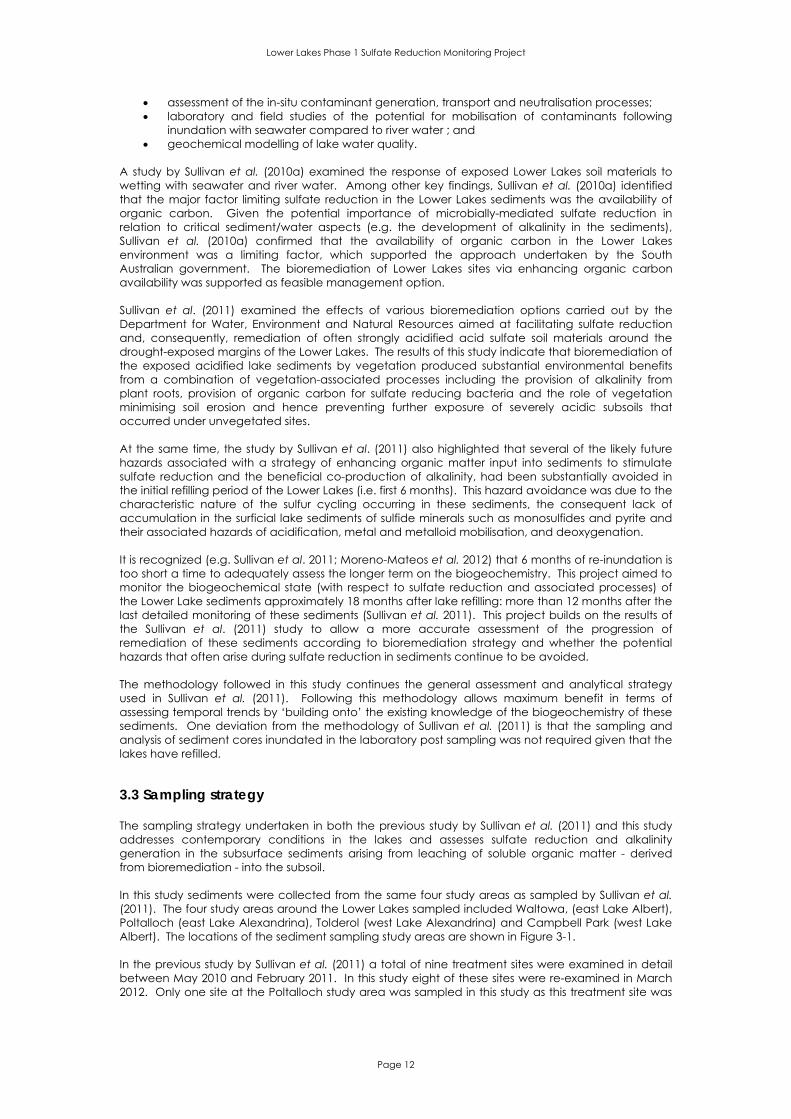
Lower Lakes Phase 1 Sulfate Reduction Monitoring Project
Page 12
assessment of the in-situ contaminant generation, transport and neutralisation processes; laboratory and field studies of the potential for mobilisation of contaminants following
inundation with seawater compared to river water ; and geochemical modelling of lake water quality.
A study by Sullivan et al. (2010a) examined the response of exposed Lower Lakes soil materials to wetting with seawater and river water. Among other key findings, Sullivan et al. (2010a) identified that the major factor limiting sulfate reduction in the Lower Lakes sediments was the availability of organic carbon. Given the potential importance of microbially-mediated sulfate reduction in relation to critical sediment/water aspects (e.g. the development of alkalinity in the sediments), Sullivan et al. (2010a) confirmed that the availability of organic carbon in the Lower Lakes environment was a limiting factor, which supported the approach undertaken by the South Australian government. The bioremediation of Lower Lakes sites via enhancing organic carbon availability was supported as feasible management option. Sullivan et al. (2011) examined the effects of various bioremediation options carried out by the Department for Water, Environment and Natural Resources aimed at facilitating sulfate reduction and, consequently, remediation of often strongly acidified acid sulfate soil materials around the drought-exposed margins of the Lower Lakes. The results of this study indicate that bioremediation of the exposed acidified lake sediments by vegetation produced substantial environmental benefits from a combination of vegetation-associated processes including the provision of alkalinity from plant roots, provision of organic carbon for sulfate reducing bacteria and the role of vegetation minimising soil erosion and hence preventing further exposure of severely acidic subsoils that occurred under unvegetated sites. At the same time, the study by Sullivan et al. (2011) also highlighted that several of the likely future hazards associated with a strategy of enhancing organic matter input into sediments to stimulate sulfate reduction and the beneficial co-production of alkalinity, had been substantially avoided in the initial refilling period of the Lower Lakes (i.e. first 6 months). This hazard avoidance was due to the characteristic nature of the sulfur cycling occurring in these sediments, the consequent lack of accumulation in the surficial lake sediments of sulfide minerals such as monosulfides and pyrite and their associated hazards of acidification, metal and metalloid mobilisation, and deoxygenation. It is recognized (e.g. Sullivan et al. 2011; Moreno-Mateos et al. 2012) that 6 months of re-inundation is too short a time to adequately assess the longer term on the biogeochemistry. This project aimed to monitor the biogeochemical state (with respect to sulfate reduction and associated processes) of the Lower Lake sediments approximately 18 months after lake refilling: more than 12 months after the last detailed monitoring of these sediments (Sullivan et al. 2011). This project builds on the results of the Sullivan et al. (2011) study to allow a more accurate assessment of the progression of remediation of these sediments according to bioremediation strategy and whether the potential hazards that often arise during sulfate reduction in sediments continue to be avoided. The methodology followed in this study continues the general assessment and analytical strategy used in Sullivan et al. (2011). Following this methodology allows maximum benefit in terms of assessing temporal trends by ‘building onto’ the existing knowledge of the biogeochemistry of these sediments. One deviation from the methodology of Sullivan et al. (2011) is that the sampling and analysis of sediment cores inundated in the laboratory post sampling was not required given that the lakes have refilled.
3.3 Sampling strategy The sampling strategy undertaken in both the previous study by Sullivan et al. (2011) and this study addresses contemporary conditions in the lakes and assesses sulfate reduction and alkalinity generation in the subsurface sediments arising from leaching of soluble organic matter - derived from bioremediation - into the subsoil. In this study sediments were collected from the same four study areas as sampled by Sullivan et al. (2011). The four study areas around the Lower Lakes sampled included Waltowa, (east Lake Albert), Poltalloch (east Lake Alexandrina), Tolderol (west Lake Alexandrina) and Campbell Park (west Lake Albert). The locations of the sediment sampling study areas are shown in Figure 3-1. In the previous study by Sullivan et al. (2011) a total of nine treatment sites were examined in detail between May 2010 and February 2011. In this study eight of these sites were re-examined in March 2012. Only one site at the Poltalloch study area was sampled in this study as this treatment site was

Lower Lakes Phase 1 Sulfate Reduction Monitoring Project
Page 13
essentially duplicated in the earlier study. A summary of the treatments examined in this study are presented in Table 3-1. Table 3-1. Summary of the treatments examined at each study area in the Lower Lakes (March 2012).
Study Area Treatment i. Phragmites bioremediation ii. Cotula bioremediation
Waltowa
iii. Juncus bioremediation
Poltalloch i. 2009 plantings of Bevy rye bioremediation i. Scald (no bioremediation) Tolderol ii. 2010 planted Juncus into 2009 plantings of Bevy rye bioremediation i. Scald (no bioremediation) Campbell Park ii. 2010 seeded with Bevy rye and Puccinellia bioremediation
Figure 3-1. Map showing study areas in the Lower Lakes (Source: Google Maps).

Lower Lakes Phase 1 Sulfate Reduction Monitoring Project
Page 14
3.4 Lower Lakes site locations and characteristics Maps showing the sampling locations in each study area and selected photographs are presented in Sections 3.4.1 to 3.4.4. Bathymetry maps of each study area are also presented in Appendix 7 (Figures 9-113 to 9-116). Historical water level and salinity data for Lake Alexandrina and Lake Albert is also included in Appendix 7 (Figures 9-117 and 9-118).
3.4.1 Waltowa, east Lake Albert study area characteristics
Figure 3-2. Waltowa sampling locations (Source: Google Maps).

Lower Lakes Phase 1 Sulfate Reduction Monitoring Project
Page 15
Figure 3-3. Sediment cores collected from the Phragmites site (left) (No MBO accumulation at this replicate site) and Cotula site (right) at Waltowa in March 2012.
Profile descriptions are presented in Appendix 1.
Figure 3-4. Sediment cores collected from the Juncus site at Waltowa in March 2012. Profile descriptions are presented in Appendix 1.
Figure 3-5. Comparison of the sediment cores collected from the Phragmites site (left core) with MBO accumulation and Cotula site (right core).
Profile descriptions are presented in Appendix 1.

Lower Lakes Phase 1 Sulfate Reduction Monitoring Project
Page 16
3.4.2 Poltalloch, east Lake Alexandrina study area characteristics
Figure 3-6. Poltalloch sampling locations (Source: Google Maps).

Lower Lakes Phase 1 Sulfate Reduction Monitoring Project
Page 17
3.4.3 Tolderol, west Lake Alexandrina study area characteristics
Figure 3-7. Tolderol sampling locations (Source: Google Maps).
Figure 3-8. Sampling at Tolderol in March 2012.

Lower Lakes Phase 1 Sulfate Reduction Monitoring Project
Page 18
Figure 3-9. Sediment core collected from the scald site (left) and iron segregation (right) at Tolderol in March 2012. Profile descriptions are presented in Appendix 1.
Figure 3-10. Iron segregations (left) and iron/jarosite (right) in the sediment core collected from the scald site at Tolderol in March 2012.
Profile descriptions are presented in Appendix 1.
Figure 3-11. Sediment cores collected from the vegetated (Juncus in Bevy rye) site at Tolderol in March 2012. Profile descriptions are presented in Appendix 1.

Lower Lakes Phase 1 Sulfate Reduction Monitoring Project
Page 19
Figure 3-12. Comparison of the sediment cores collected from the vegetated (left core) and scald (right core) sites. Profile descriptions are presented in Appendix 1.
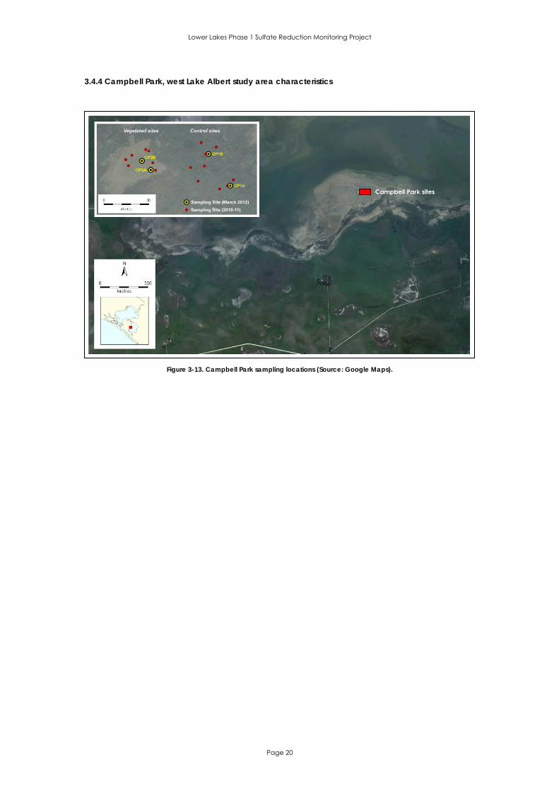
Lower Lakes Phase 1 Sulfate Reduction Monitoring Project
Page 20
3.4.4 Campbell Park, west Lake Albert study area characteristics
Figure 3-13. Campbell Park sampling locations (Source: Google Maps).
Lower Lakes Phase 1 Sulfate Reduction Monitoring Project
Page 21
4.0 Materials and methods The methodology followed in this study continues the general assessment and analytical strategy used in Sullivan et al. (2011). Following this methodology allows maximum benefit in terms of assessing temporal trends by ‘building onto’ the existing knowledge of the biogeochemistry of these sediments. One deviation from the methodology of Sullivan et al. (2011) is that the sampling and analysis of sediment cores inundated in the laboratory post sampling was not required given that the lakes have refilled.
4.1 Field sampling of soils Field sampling at the four Lower Lakes study areas was undertaken between 29th and 31st March 2012. In the previous study by Sullivan et al. (2011), field sampling at the same study areas was undertaken before seeding/planting in May 2010, and then undertaken on three separate occasions (i.e. August 2010, November 2010 and February 2011). A summary of the sampling dates for this and the previous study are presented below in Table 4-1.
Table 4-1. Sampling dates for the field sulfate rate assessment and soil profile sampling (May 2010 – March 2012).
Season (Date) Field Sulfate Rate
Assessment Soil Profile Sampling
Late Autumn (21st - 23rd May 2010)
Late Winter (28th - 31stAugust 2010)
Late Spring (21st – 24th November 2010)
Late Summer (14th – 17th February 2011)
Mid Autumn (29th – 31st March 2012)
The sampling dates in the earlier study were originally chosen to coincide with four growth stages of the annual vegetation to be planted during 2010: before planting, early-growth, near-maturity and post-maturity. However, flooding in the lakes during June-August 2010 impeded the establishment of the seeded/planted areas in Lake Alexandrina, and the development of the seeded areas at the Campbell Park study area beyond early-growth stage after the inundation of Lake Albert that occurred post-August 2010. In this study duplicate intact sediment cores were collected using a 5 cm diameter push-tube coring device from two replicate sampling sites from each treatment/location to a depth of 40 cm. Each core was collected within 4 m of the initial site sampled in the previous study (Sullivan et al. 2011) to ensure that the detection of any changes in soil properties since the last sampling time was optimised. A surficial monosulfidic black ooze (MBO) was observed at one of the Waltowa Phragmites sites and was sampled separately. All sediment samples were frozen after sub-sampling and field measurements. A soil description together with pH/Eh data for each horizon collected is presented in Appendix 1 (Table 9-1). The pH and Eh were determined using calibrated electrodes linked to a TPS 90-FLMV multi-parameter meter; Eh measurements are presented versus the standard hydrogen electrode. The global positioning system (GPS) coordinates for each site are also presented in Appendix 1 (Table 9-1).

Lower Lakes Phase 1 Sulfate Reduction Monitoring Project
Page 22
Figure 4-1. Sediment sampling at Tolderol (March 2012).

Lower Lakes Phase 1 Sulfate Reduction Monitoring Project
Page 23
4.2 Laboratory analysis methods
4.2.1 General comments All laboratory glassware and plastic-ware were cleaned by soaking in 5% (v/v) HCl for at least 24 hours, followed by repeated rinsing with deionised water. Reagents were analytical grade and all reagent solutions were prepared with deionised water (milliQ). All solid-phase results are presented on a dry weight basis (except where otherwise noted).
4.2.2 Sediment analyses The parameters measured on the sediment/soil layers collected included:
Moisture content pH (1:5 soil:water) EC (1:5 soil:water) RIS (CRS, S(0) and AVS) Total C and N (by LECO) pH (1:40 soil: I.0 M KCl) TAA (only if pHKCl is <6.5) ANC (only if pHKCl is >6.5) TAAlk (only if pHKCl is >6.5) RA (only if pHKCl is <4.5) HCl extractable metals/metalloids Organic matter availability and quantity Sulfate reduction rates
The sediment moisture content was determined by weight loss due to drying at 105oC. Sediments for further analysis (with the exception of sediments analysed for reduced inorganic sulfur (RIS) and sulfate reduction rates) were oven-dried at 80oC and sieved (< 2 mm) prior to being ring mill ground. The acid-volatile sulfide (AVS), elemental sulfur (S(0)) and pyritic sulfur fractions were determined using a sequential extraction procedure on duplicate frozen sub-samples. The AVS fraction was initially extracted via a cold diffusion procedure, with the use of ascorbic acid to prevent interferences from ferric iron (Fe (III)) (Burton et al. 2007). The solid phase S(0) fraction was extracted using methanol as a solvent and quantified by high-performance liquid chromatography (HPLC) (McGuire and Hamers 2000). The remaining RIS fraction (i.e. pyritic sulfur) was determined using the chromium reduction analysis method of Burton et al. (2008b). The methodology followed in the determination of the sulfate reduction rates is summarised in Section 4.2.3. Electrical conductivity (EC) and pH were determined by direct insertion of calibrated electrodes into a 1:5 soil:water extract linked to a TPS WP-81 meter. Total carbon (%C) and total nitrogen (%N) were measured on powdered oven-dried samples by combustion using a LECO-CNS 2000 analyser. The potassium chloride (KCl) extractable pH (pHKCl) was measured in a 1:40 1.0 M KCl extract (Method Code 23A), and the titratable actual acidity (TAA) (i.e. sum of soluble and exchangeable acidity) was determined by titration of the KCl extract to pH 6.5 (Method Code 23F) (Ahern et al. 2004). Titratable actual acidity is a measure of the actual acidity in soil materials. The titratable actual alkalinity (TAAlk) was measured on samples where pHKCl was >6.5 (Sullivan et al. 2010b). Titratable actual alkalinity where the suspension is titrated with 0.05 M hydrochloric acid (HCl) down to pH 6.5 is the reverse of the TAA method. The acid neutralising capacity (ANCBT) was quantified on the <0.5 mm sieved soil fraction (only if pHKCl is >6.5) using a standard back-titration determination (Method Code 19A2) (Ahern et al. 2004). The retained acidity (RA) was determined from the difference between 4.0 M HCl extractable sulfur (SHCl) and 1.0 M KCl extractable sulfur (SKCl) when the sample pHKCl was < 4.5 (Method Code 20J) (Ahern et al. 2004). The retained acidity identifies stored soil acidity in the form of jarosite and similar relatively insoluble iron and aluminium hydroxy sulfate compounds (Ahern et al. 2004). The net acidity was estimated by the acid-base account method of Ahern et al. (2004). Reactive metals and metalloids (Fe, Al, Ag, As, Pb, Cd, Cr, Cu, Mn, Ni, Se and Zn) were extracted using 1.0 M HCl and analysed using ICP-MS (Inductively Coupled Plasma - Mass Spectrometry). The organic matter availability and quantity (i.e. total organic C, hydrolysable C and non-hydrolysable C) were measured after the 1.0 M HCl method described by Silveira et al. (2008). The total organic carbon (TOC) content was determined by a LECO-CNS 2000 analyser following the

Lower Lakes Phase 1 Sulfate Reduction Monitoring Project
Page 24
removal of inorganic carbon by treatment with 1.0 M HCl. The non-hydrolysable organic carbon content was determined by a LECO-CNS 2000 analyser following treatment with 6.0 M HCl at 105oC for 2 hours. The hydrolysable organic carbon content was determined from the difference between the TOC and the non-hydrolysable carbon fractions. All sediment data are presented in Appendix 2 (Tables 9-2 to 9-9).
4.2.3 Sulfate reduction analyses In-situ SO42--reduction rates (SRR) were determined following the same methodology previously used in Sullivan et al. (2011). Sulfate reduction rates were determined using a radiotracer (35SO42-) incubation approach (Fossing and Jørgensen 1989) in which short-term products of sulfate reduction (i.e. iron-monosulfides, elemental sulfur and pyrite) were also investigated. Sediment profiles were collected using a 5 cm diameter push-tube coring device. The rate of sulfate reduction was measured at the surface in 2.5 cm increments (i.e. 0-2.5 cm, 2.5-5.0 cm), then in 5 cm increments to 20 cm, and 10 cm increments from 20 cm to 40 cm. Four replicate soil sub-samples for each soil layer were collected using 3 mL polypropylene syringes (with the distal end removed). After collection, each soil sample was immediately sealed within the 3 mL syringe using Parafilm and was subsequently injected with 100 kBq of carrier-free 35SO42-. Three replicates from each depth interval were incubated at ambient temperature for 24 hours. These incubations were terminated by freezing the sealed syringes. In addition to the triplicate 24 hour incubations, a single replicate for selected soil samples also served as a time zero blank (i.e. this sample was frozen immediately after injection of 35SO42-). The RIS speciation of the radiolabelled samples was determined by selective, sequential extraction of iron-monosulfides, elemental sulfur (S(0)) and pyrite (Burton et al. 2007, 2009). Iron-monosulfides, defined operationally as AVS, were extracted by shaking (150 rpm) 0.5 grams of sediment with 10 mL of 6.0 M HCl/0.1 M ascorbic acid in gas-tight 55 cm3 polypropylene reactors for 18 hours (Burton et al. 2007). The use of ascorbic acid during this extraction prevents interferences from Fe(III) minerals, which can otherwise lead to S(0) formation (Hsieh et al. 2002). The evolved hydrogen sulfide (H2S(g)) was trapped in 7 mL of 3% zinc acetate in 2.0 M sodium hydroxide (NaOH), and subsequently quantified via iodometric titration. Elemental S was then extracted from the AVS-extracted sample by shaking the sediment with 10 mL of methanol for 16 hours. An aliquot of the methanol extract was analysed for S(0) by HPLC with a Dionex UltiMate 3000 system. Residual S(0) was then removed from the sediment sample by three rinses with 25 mL of acetone, and a final rinse with 20 mL of ethanol. Each rinse involved 5 to 10 minutes of shaking, with the sediment and acetone/ethanol phases separated between rinses by centrifugation at 4000 rpm for 10 minutes. Pyritic sulfur in the residual AVS- and S(0)-extracted sediment was then quantified as chromium reducible sulfur (CRS) using the method of Burton et al. (2008b). The incorporation of 35S into each of the three RIS fractions was determined by liquid-scintillation counting using a Perkin-Elmer microbeta counter (with Perkin-Elmer UltimaGold scintillation fluid). The SO42--reduction rate was determined by the sum of 35S incorporated into AVS, S(0) and CRS according to:
06.112
4
dSO
A
baSRR nmol/g/day
Where a is the radioactivity of the individual RIS species per mass of soil subjected to the incubation, b is the mean radioactivity of the time zero blanks, A is the radioactivity of the added 35SO42- per mass of soil, [SO42-] is the sulfate concentration per mass of soil (nmol/g), d is the incubation time in days, and 1.06 is the isotopic fractionation factor. It is important to note that using 35S incubations to quantify the importance of short-term sulfate reduction biomineralisation products is complicated by possible isotopic exchange of 35S amongst separate RIS species. More specifically, absolute quantitative distinction between the in-situ formation rates of S(0) and AVS may be unreliable due to partial isotopic exchange of 35S (Fossing et al. 1992). On the other hand, it is well established that isotopic exchange of 35S does not occur between pyrite and other RIS species over a 24 hour period (Fossing et al. 1992). Therefore, differential incorporation of 35S into the AVS versus S(0) pools must be interpreted cautiously, whereas 35S incorporation into CRS can be soundly interpreted as real short-term pyrite formation (Burton et al. 2011). All sulfate reduction data are presented in Appendix 3 (Tables 9-10 to 9-25).

Lower Lakes Phase 1 Sulfate Reduction Monitoring Project
Page 25
4.2.4 Pore-water analyses Pore-waters were extracted after centrifuging the soil samples at 3,500 rpm for 15 minutes. The parameters measured on the pore-water collected included:
Redox potential (Eh) pH Electrical conductivity (EC) Alkalinity Dissolved sulfide Total dissolved iron (Fe3+ + Fe2+) Soluble chloride and sulfate Soluble cations (Ca, Mg, Na, K) Nutrients (orthophosphate, nitrate, nitrite, and ammonia)
Redox potential, pH and electrical conductivity were immediately measured on unfiltered pore-water samples, and all other properties were determined on filtered (0.45 µm) samples. Redox potential (Eh) was determined using a calibrated electrode linked to a TPS smartCHEM-LAB laboratory analyser; Eh measurements are presented versus the standard hydrogen electrode. Electrical conductivity (EC) and pH were determined using calibrated electrodes linked to a TPS WP-81 meter. Alkalinity, dissolved sulfide and total iron (Fe2+ + Fe3+) were fixed immediately after sampling. The total iron trap was made up from a phenanthroline solution with an ammonium acetate buffer and hydroxylamine solution (APHA 2005). Bromophenol blue traps were used for alkalinity (Sarazin et al. 1999) and alkalinity standards were determined with 0.01 M HCl using the Gran procedure (Stumm and Morgan 1996). The dissolved sulfide fraction was trapped in an alkaline zinc acetate trap prior to determination by the spectrophotometric method of Cline (1969). The alkalinity, dissolved sulfide and iron concentrations were all quantified colorimetrically using a Varian Cary 50 UV-Visible spectrophotometer. Major cations and anions (Na+, K+, Ca2+, Mg2+, SO42-, Cl-) were analysed by ICP-OES (Inductively Coupled Plasma - Optical Emission Spectrometry). Nutrients (orthophosphate, nitrate, nitrite, and ammonia) were analysed turbidimetrically using flow-injection analysis (FIA) colorimetry (Lachat QuikChem 8000) (APHA 2005). All pore-water data are presented in Appendix 4 (Tables 9-26 to 9-33) and Appendix 5 (Figures 9-1 to 9-64).
4.2.5 Expression of results The means (Av.) and the standard deviations for triplicates (± SD) are presented in tables in this document with graphs given to illustrate certain points. The standard errors (SE) are presented on many of the graphs.
4.2.6 Quality assurance and quality control For all tests and analyses, the Quality Assurance and Quality Control procedures were equivalent to those endorsed by NATA (National Association of Testing Authorities). The standard procedures followed included the monitoring of blanks, duplicate analysis of at least 1 in 10 samples, and the inclusion of standards in each batch. Blanks were collected for laboratory or field samples to examine whether contaminants had been introduced to the sample. Reagent blanks and method blanks were prepared and analysed for each method. All blanks examined here were either at, or very close to, the limits of detection. Calibrations were performed on matrix-matched solutions and these were analysed along with standard solutions and the tested analytes. These calibrations and checks confirmed the methodology and the proper functioning of the analytical instruments. Duplicates were prepared for all experiments and analysed separately. Selected analytical duplicate samples were prepared by dividing a test sample into two, then analysing these sub-samples separately. On average, the frequencies of quality control samples processed were: 10%

Lower Lakes Phase 1 Sulfate Reduction Monitoring Project
Page 26
blanks, ≥ 10% laboratory duplicates, and 5% laboratory controls. The analytical precision was ±10% for all analyses.

Lower Lakes Phase 1 Sulfate Reduction Monitoring Project
Page 27
5.0 Results 5.1 General sediment condition
5.1.1 Waltowa
5.1.1.1 pH(1:1, soil:water) and TAA All sites initially (i.e. before refilling in August 2010) had slightly acidic subsoil layers from 10 – 40 cm, especially the site under Cotula where the pH in the 20 – 30 cm layer had a pH of ~4 (Figures 5-1 – 5-3). Upon near lake filling in August 2010 the pHs of these soil layers dropped considerably probably due to acidity exchange from the soil from the inundating waters. The two treatment sites that had Aglime previously applied to the surface (i.e. the Phragmites and Juncus treatments) displayed surface pHs of about 8 - 8.5 initially, but when their sediment surfaces became and remained saturated the pHs of these layers were thereafter maintained at a pH of ~ 7. In the unlimed Cotula treatment site the pH of the surface layer initially decreased from ~ 7 to ~ 5 from May 2010 to August 2010, but thereafter increased to ~pH 7 under the inundated conditions. Under all treatments at this study area and at each depth the pH of the sediment had increased by ~ 0.5 of a unit since last sampled in February 2011.
0
5
10
15
20
25
30
35
40
2 4 6 8 10
Depth (cm)
pH (1:1 soil:water)
August 2010
February 2011
March 2012
MBO March 2012
Figure 5-1. Waltowa field pH dynamics at the established Phragmites site (August 2010, February 2011 and March 2012).
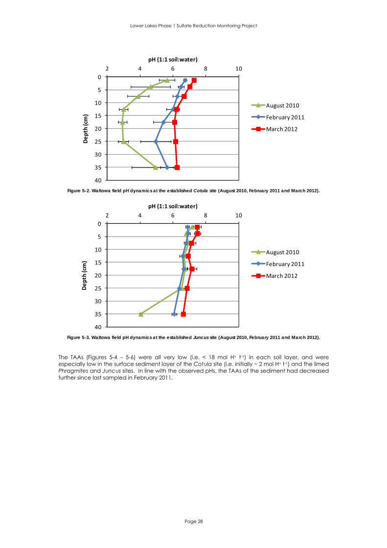
Lower Lakes Phase 1 Sulfate Reduction Monitoring Project
Page 28
0
5
10
15
20
25
30
35
40
2 4 6 8 10
Depth (cm)
pH (1:1 soil:water)
August 2010
February 2011
March 2012
Figure 5-2. Waltowa field pH dynamics at the established Cotula site (August 2010, February 2011 and March 2012).
0
5
10
15
20
25
30
35
40
2 4 6 8 10
Depth (cm)
pH (1:1 soil:water)
August 2010
February 2011
March 2012
Figure 5-3. Waltowa field pH dynamics at the established Juncus site (August 2010, February 2011 and March 2012).
The TAAs (Figures 5-4 – 5-6) were all very low (i.e. < 18 mol H+ t-1) in each soil layer, and were especially low in the surface sediment layer of the Cotula site (i.e. initially ~ 2 mol H+ t-1) and the limed Phragmites and Juncus sites. In line with the observed pHs, the TAAs of the sediment had decreased further since last sampled in February 2011.

Lower Lakes Phase 1 Sulfate Reduction Monitoring Project
Page 29
0
5
10
15
20
25
30
35
40
0 5 10 15
Depth (cm)
TAA (mol H+/t)
May 2010
August 2010
November 2010
February 2011
March 2012
MBO March 2012
Figure 5-4. Waltowa TAA dynamics at the established Phragmites site (May 2010 – March 2012).
0
5
10
15
20
25
30
35
40
0 5 10 15
Depth (cm)
TAA (mol H+/t)
May 2010
August 2010
November 2010
February 2011
March 2012
Figure 5-5. Waltowa TAA dynamics at the established Cotula site (May 2010 – March 2012).
0
5
10
15
20
25
30
35
40
0 5 10 15
Depth (cm)
TAA (mol H+/t)
May 2010
August 2010
November 2010
February 2011
March 2012
Figure 5-6. Waltowa TAA dynamics at the established Juncus site (May 2010 – March 2012).

Lower Lakes Phase 1 Sulfate Reduction Monitoring Project
Page 30
5.1.1.2 Redox potential (Eh) All sites initially (i.e. in May 2010) had oxic conditions (Figures 5-7 – 5-9), but during the inundation process increasingly reductive conditions developed initially most strongly in the subsurface layers (August 2010) but then in the whole profile down to 40 cm during the inundations. In the surface sediments the Ehs were ~ 0 mV during the February 2011 sampling in all treatment sites. Since last sampled in February 2011 the < 20 cm deep sediments under all treatments at this study area had further decreased. However, the Eh in the surface soil layers at both the Cotula and Juncus sites had increased slightly, whereas the very low Eh in the surface soil layers at the Phragmites sites had been maintained during this period.
0
5
10
15
20
25
30
35
40
‐200 0 200 400 600 800
Depth (cm)
Eh (mV)
May 2010
August 2010
November 2010
February 2011
March 2012
MBO March 2012
Figure 5-7. Waltowa field Eh dynamics at the established Phragmites site (May 2010 – March 2012).
0
5
10
15
20
25
30
35
40
‐200 0 200 400 600 800
Depth (cm)
Eh (mV)
May 2010
August 2010
November 2010
February 2011
March 2012
Figure 5-8. Waltowa field Eh dynamics at the established Cotula site (May 2010 – March 2012).

Lower Lakes Phase 1 Sulfate Reduction Monitoring Project
Page 31
0
5
10
15
20
25
30
35
40
‐200 0 200 400 600 800
Depth (cm)
Eh (mv)
May 2010
August 2010
November 2010
February 2011
March 2012
Figure 5-9. Waltowa field Eh dynamics at the established Juncus site (May 2010 – March 2012).
5.1.1.3 Electrical conductivity (EC) The salinity (i.e. EC) in the sediments has decreased only slightly from before inundation to after prolonged inundation. As shown in Figures 5-10 – 5-12 the salinity in all treatments was between 700 and 1500 µS cm-1 in the surface layers down to ~30 cm depth but increased to up to 3,000 µS cm-1 in the 30-40 cm layer.
0
5
10
15
20
25
30
35
40
0 2000 4000 6000 8000 10000
Depth (cm)
EC (µS/cm)
May 2010
August 2010
November 2010
February 2011
March 2012
MBO March 2012
Figure 5-10. Waltowa EC dynamics at the established Phragmites site (May 2010 – March 2012).

Lower Lakes Phase 1 Sulfate Reduction Monitoring Project
Page 32
0
5
10
15
20
25
30
35
40
0 1000 2000 3000 4000
Depth (cm)
EC (µS/cm)
May 2010
August 2010
November 2010
February 2011
March 2012
Figure 5-11. Waltowa EC dynamics at the established Cotula site (May 2010 – March 2012).
0
5
10
15
20
25
30
35
40
0 1000 2000 3000 4000
Depth (cm)
EC (µS/cm)
May 2010
August 2010
November 2010
February 2011
March 2012
Figure 5-12. Waltowa EC dynamics at the established Juncus site (May 2010 – March 2012).
5.1.1.4 Chromium reducible sulfur (CRS) The pyritic sulfur content in the top 30 cm of sediment was very low in all sites prior to inundation (Figures 5-13 – 5-15). The deeper soil materials contained pyrite at all sites. There was evidence of accumulation of appreciable concentrations reduced inorganic sulfides (i.e. up to 0.08% S as pyrite), especially in the Phragmites site profile and the Cotula surface layer after 6 months of inundation (i.e. the February 2011 data). With another 13 months of inundation pyrite continued to accumulate in the upper surface layers under the Phragmites treatment, but declined in the Cotula upper surface layer in which it had previously accumulated. The concentration of Acid Volatile Sulfur (i.e. monosulfides) has trended in parallel with the pyrite concentrations (Figures 5-16 – 5-18). It is of importance that an appreciable depth of Monosulfidic Black Ooze (MBO) had begun to accumulate by March 2012 on the surface of the Phragmites treatment. Elemental sulfur (Figure 5-19) was still present in the surficial layers at each site but in very low concentrations.
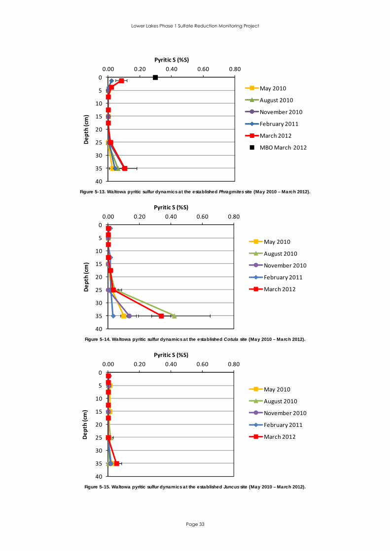
Lower Lakes Phase 1 Sulfate Reduction Monitoring Project
Page 33
0
5
10
15
20
25
30
35
40
0.00 0.20 0.40 0.60 0.80
Depth (cm)
Pyritic S (%S)
May 2010
August 2010
November 2010
February 2011
March 2012
MBO March 2012
Figure 5-13. Waltowa pyritic sulfur dynamics at the established Phragmites site (May 2010 – March 2012).
0
5
10
15
20
25
30
35
40
0.00 0.20 0.40 0.60 0.80
Depth (cm)
Pyritic S (%S)
May 2010
August 2010
November 2010
February 2011
March 2012
Figure 5-14. Waltowa pyritic sulfur dynamics at the established Cotula site (May 2010 – March 2012).
0
5
10
15
20
25
30
35
40
0.00 0.20 0.40 0.60 0.80
Depth (cm)
Pyritic S (%S)
May 2010
August 2010
November 2010
February 2011
March 2012
Figure 5-15. Waltowa pyritic sulfur dynamics at the established Juncus site (May 2010 – March 2012).

Lower Lakes Phase 1 Sulfate Reduction Monitoring Project
Page 34
0
5
10
15
20
25
30
35
40
0.00 0.05 0.10 0.15 0.20
Depth (cm)
AVS (%S)
May 2010
August 2010
November 2010
February 2011
March 2012
MBO March 2012
Figure 5-16. Waltowa AVS dynamics at the established Phragmites site (May 2010 – March 2012).
0
5
10
15
20
25
30
35
40
0.00 0.05 0.10 0.15 0.20
Depth (cm)
AVS (%S)
May 2010
August 2010
November 2010
February 2011
March 2012
Figure 5-17. Waltowa AVS dynamics at the established Cotula site (May 2010 – March 2012).
0
5
10
15
20
25
30
35
40
0.00 0.05 0.10 0.15 0.20
Depth (cm)
AVS (%S)
May 2010
August 2010
November 2010
February 2011
March 2012
Figure 5-18. Waltowa AVS dynamics at the established Juncus site (May 2010 – March 2012).
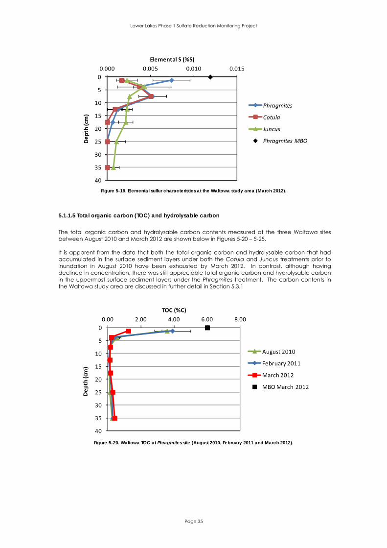
Lower Lakes Phase 1 Sulfate Reduction Monitoring Project
Page 35
0
5
10
15
20
25
30
35
40
0.000 0.005 0.010 0.015
Depth (cm)
Elemental S (%S)
Phragmites
Cotula
Juncus
Phragmites MBO
Figure 5-19. Elemental sulfur characteristics at the Waltowa study area (March 2012).
5.1.1.5 Total organic carbon (TOC) and hydrolysable carbon The total organic carbon and hydrolysable carbon contents measured at the three Waltowa sites between August 2010 and March 2012 are shown below in Figures 5-20 – 5-25. It is apparent from the data that both the total organic carbon and hydrolysable carbon that had accumulated in the surface sediment layers under both the Cotula and Juncus treatments prior to inundation in August 2010 have been exhausted by March 2012. In contrast, although having declined in concentration, there was still appreciable total organic carbon and hydrolysable carbon in the uppermost surface sediment layers under the Phragmites treatment. The carbon contents in the Waltowa study area are discussed in further detail in Section 5.3.1
0
5
10
15
20
25
30
35
40
0.00 2.00 4.00 6.00 8.00
Depth (cm)
TOC (%C)
August 2010
February 2011
March 2012
MBO March 2012
Figure 5-20. Waltowa TOC at Phragmites site (August 2010, February 2011 and March 2012).
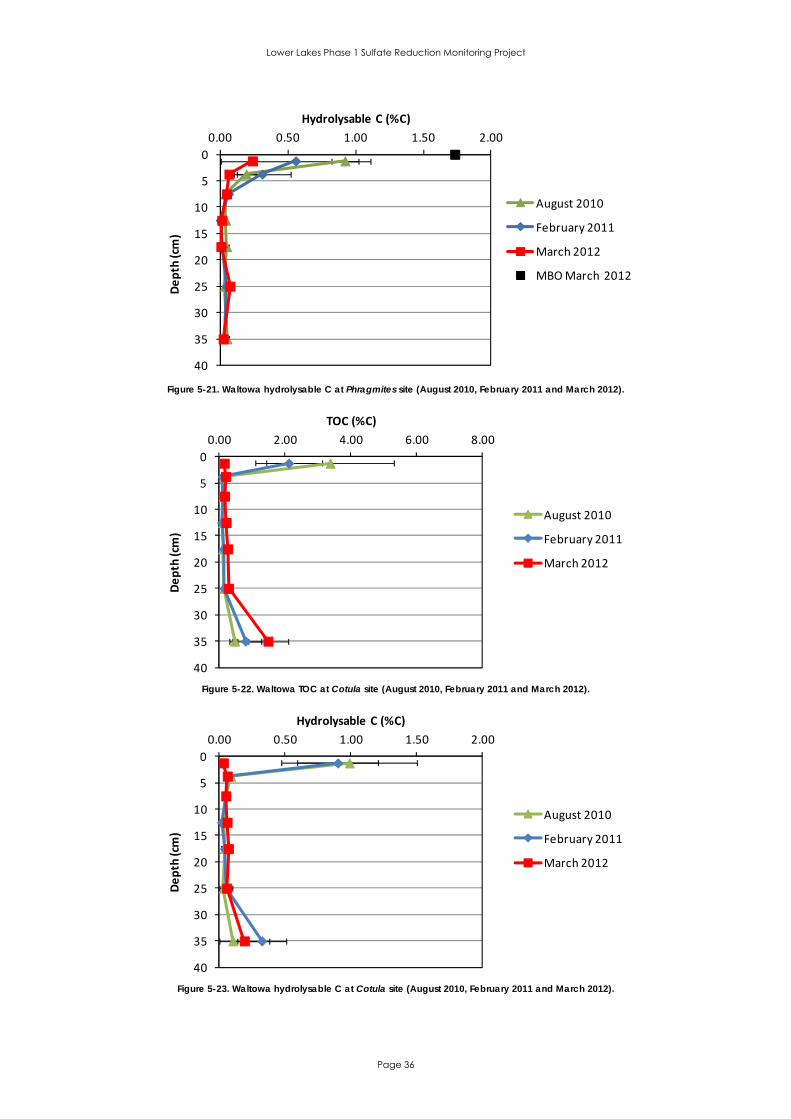
Lower Lakes Phase 1 Sulfate Reduction Monitoring Project
Page 36
0
5
10
15
20
25
30
35
40
0.00 0.50 1.00 1.50 2.00
Depth (cm)
Hydrolysable C (%C)
August 2010
February 2011
March 2012
MBO March 2012
Figure 5-21. Waltowa hydrolysable C at Phragmites site (August 2010, February 2011 and March 2012).
0
5
10
15
20
25
30
35
40
0.00 2.00 4.00 6.00 8.00
Depth (cm)
TOC (%C)
August 2010
February 2011
March 2012
Figure 5-22. Waltowa TOC at Cotula site (August 2010, February 2011 and March 2012).
0
5
10
15
20
25
30
35
40
0.00 0.50 1.00 1.50 2.00
Depth (cm)
Hydrolysable C (%C)
August 2010
February 2011
March 2012
Figure 5-23. Waltowa hydrolysable C at Cotula site (August 2010, February 2011 and March 2012).

Lower Lakes Phase 1 Sulfate Reduction Monitoring Project
Page 37
0
5
10
15
20
25
30
35
40
0.00 2.00 4.00 6.00 8.00
Depth (cm)
TOC (%C)
August 2010
February 2011
March 2012
Figure 5-24. Waltowa TOC at Juncus site (August 2010, February 2011 and March 2012).
0
5
10
15
20
25
30
35
40
0.00 0.50 1.00 1.50 2.00
Depth (cm)
Hydrolysable C (%C)
August 2010
February 2011
March 2012
Figure 5-25. Waltowa hydrolysable C at Juncus site (August 2010, February 2011 and March 2012).

Lower Lakes Phase 1 Sulfate Reduction Monitoring Project
Page 38
5.1.2 Poltalloch
5.1.2.1 pH(1:1, soil:water) and TAA Since re-inundation in August 2010, the pHs of the upper 20 cm of sediment has increased slightly from a pH of 6.5 - 7 to a pH of 7 -7.3 (Figure 5-26). Although the pHs at this study area were < 4 in the 20 – 30 cm layer prior to inundation and after 6 months of inundation, the subsequent 13 months of inundation have resulted in substantial pH increases in these layers to between pH 5.5 -6.
0
5
10
15
20
25
30
35
40
2 4 6 8 10
Depth (cm)
pH (1:1 soil:water)
August 2010
February 2011
March 2012
Figure 5-26. Poltalloch field pH dynamics at the Bevy rye site (August 2010, February 2011 and March 2012).
The TAAs (Figure 5-27) were all very low (i.e. < 5 mol H+ t-1) in each soil layer, and were especially low (i.e. <2 mol H+ t-1) in the surface sediment layers prior to, during, and post inundation.
0
5
10
15
20
25
30
35
40
0 5 10 15
Depth (cm)
TAA (mol H+/t)
May 2010
August 2010
November 2010
February 2011
March 2012
Figure 5-27. Poltalloch TAA dynamics at the Bevy rye site (May 2010 – March 2012).

Lower Lakes Phase 1 Sulfate Reduction Monitoring Project
Page 39
5.1.2.2 Redox potential (Eh) Initially (i.e. in May 2010) the site had oxic conditions (Figure 5-28), but during the inundation process increasingly reductive conditions developed throughout the whole profile down to 40 cm and have further decreased slightly during the prolonged inundation.
0
5
10
15
20
25
30
35
40
0 200 400 600 800
Depth (cm)
Eh (mV)
May 2010
August 2010
November 2010
February 2011
March 2012
Figure 5-28. Poltalloch field Eh dynamics at the Bevy rye site (May 2010 – March 2012).
5.1.2.3 Electrical conductivity (EC) The salinity (i.e. EC) did not change appreciably from before inundation to after prolonged inundation. As shown in Figure 5-29 the salinity in the surface layers fell from ~500 µS cm-1 to ~100 µS cm-1 after prolonged inundation. The salinities of the sediment layers gradually increase with depth. At the March 2012 sampling the EC in the lowest layer was ~700 µS cm-1 at 40 cm.
0
5
10
15
20
25
30
35
40
0 500 1000 1500
Depth (cm)
EC (µS/cm)
May 2010
August 2010
November 2010
February 2011
March 2012
Figure 5-29. Poltalloch EC dynamics at the Bevy rye site (May 2010 – March 2012).
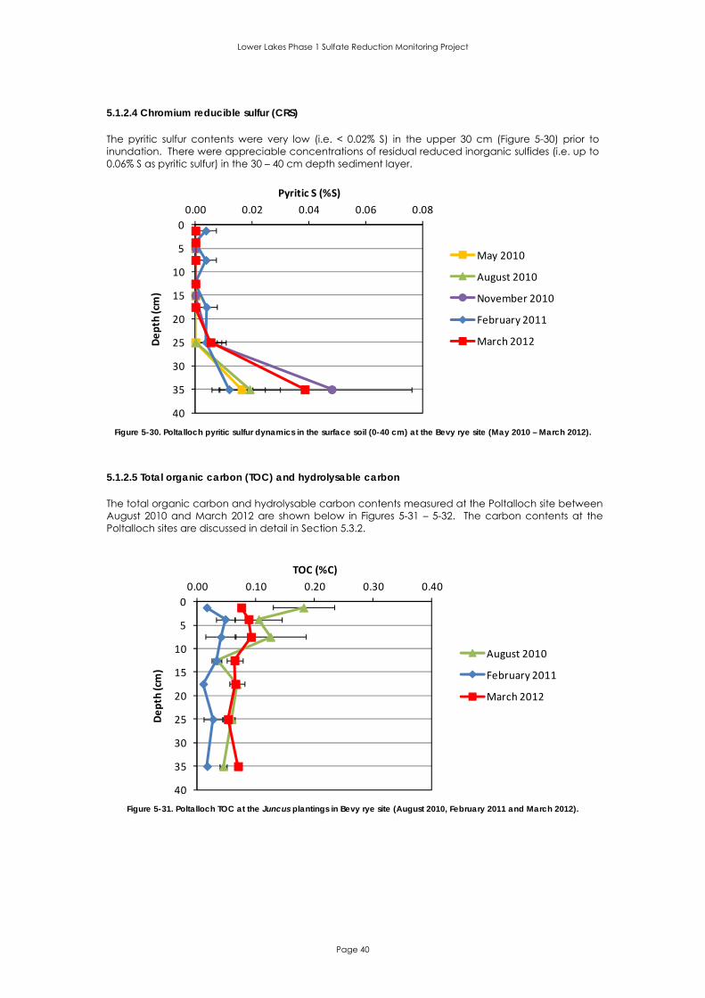
Lower Lakes Phase 1 Sulfate Reduction Monitoring Project
Page 40
5.1.2.4 Chromium reducible sulfur (CRS) The pyritic sulfur contents were very low (i.e. < 0.02% S) in the upper 30 cm (Figure 5-30) prior to inundation. There were appreciable concentrations of residual reduced inorganic sulfides (i.e. up to 0.06% S as pyritic sulfur) in the 30 – 40 cm depth sediment layer.
0
5
10
15
20
25
30
35
40
0.00 0.02 0.04 0.06 0.08
Depth (cm)
Pyritic S (%S)
May 2010
August 2010
November 2010
February 2011
March 2012
Figure 5-30. Poltalloch pyritic sulfur dynamics in the surface soil (0-40 cm) at the Bevy rye site (May 2010 – March 2012).
5.1.2.5 Total organic carbon (TOC) and hydrolysable carbon The total organic carbon and hydrolysable carbon contents measured at the Poltalloch site between August 2010 and March 2012 are shown below in Figures 5-31 – 5-32. The carbon contents at the Poltalloch sites are discussed in detail in Section 5.3.2.
0
5
10
15
20
25
30
35
40
0.00 0.10 0.20 0.30 0.40
Depth (cm)
TOC (%C)
August 2010
February 2011
March 2012
Figure 5-31. Poltalloch TOC at the Juncus plantings in Bevy rye site (August 2010, February 2011 and March 2012).

Lower Lakes Phase 1 Sulfate Reduction Monitoring Project
Page 41
0
5
10
15
20
25
30
35
40
0.00 0.05 0.10 0.15 0.20
Depth (cm)
Hydrolysable C (%C)
August 2010
February 2011
March 2012
Figure 5-32. Poltalloch hydrolysable C at the Juncus plantings in Bevy rye site
(August 2010, February 2011 and March 2012).

Lower Lakes Phase 1 Sulfate Reduction Monitoring Project
Page 42
5.1.3 Tolderol
5.1.3.1 pH(1:1, soil:water) and TAA The control site (from 0 - 40 cm) and the Bevy rye site (only 10 - 40 cm) initially were acidic (pH < ~4) prior to inundation (Figures 5-33 – 5-34). Upon lake filling in August 2010 the pHs of the surface soil layers down to 40 cm depth in the control site further acidified considerably likely due to acidity exchange from the soil from the inundating waters. This acidification upon inundation effect was confined to the 20 – 50 cm layer in the Bevy rye site. During prolonged inundation of both sites since August 2010 the pHs of sediments under both sites increased although this was initially most pronounced in the surficial sediment layers under the Bevy rye site in comparison with the control site.
0
5
10
15
20
25
30
35
40
2 4 6 8 10
Depth (cm)
pH (1:1 soil:water)
August 2010
February 2011
March 2012
Figure 5-33. Tolderol field pH dynamics at the control site (August 2010, February 2011 and March 2012).
0
5
10
15
20
25
30
35
40
2 4 6 8 10
Depth (cm)
pH (1:1 soil:water)
August 2010
February 2011
March 2012
Figure 5-34. Tolderol field pH dynamics at the Juncus in Bevy rye site (August 2010, February 2011 and March 2012).

Lower Lakes Phase 1 Sulfate Reduction Monitoring Project
Page 43
The TAAs (Figures 5-35 – 5-36) were all very low (i.e. < 18 mol H+ t-1) in each soil layer, and were especially low initially in the surface sediment layers of the Bevy rye treatment (i.e. initially ~3 mol H+ t-
1). The TAAs have generally decreased further with prolonged exposure in all soil layers of each site.
0
5
10
15
20
25
30
35
40
0 5 10 15 20 25
Depth (cm)
TAA (mol H+/t)
May 2010
August 2010
November 2010
February 2011
March 2012
Figure 5-35. Tolderol TAA dynamics at the control site (May 2010 – March 2012).
0
5
10
15
20
25
30
35
40
0 5 10 15 20 25
Depth (cm)
TAA (mol H+/t)
May 2010
August 2010
November 2010
February 2011
March 2012
Figure 5-36. Tolderol TAA dynamics at the Juncus in Bevy rye site (May 2010 – March 2012).
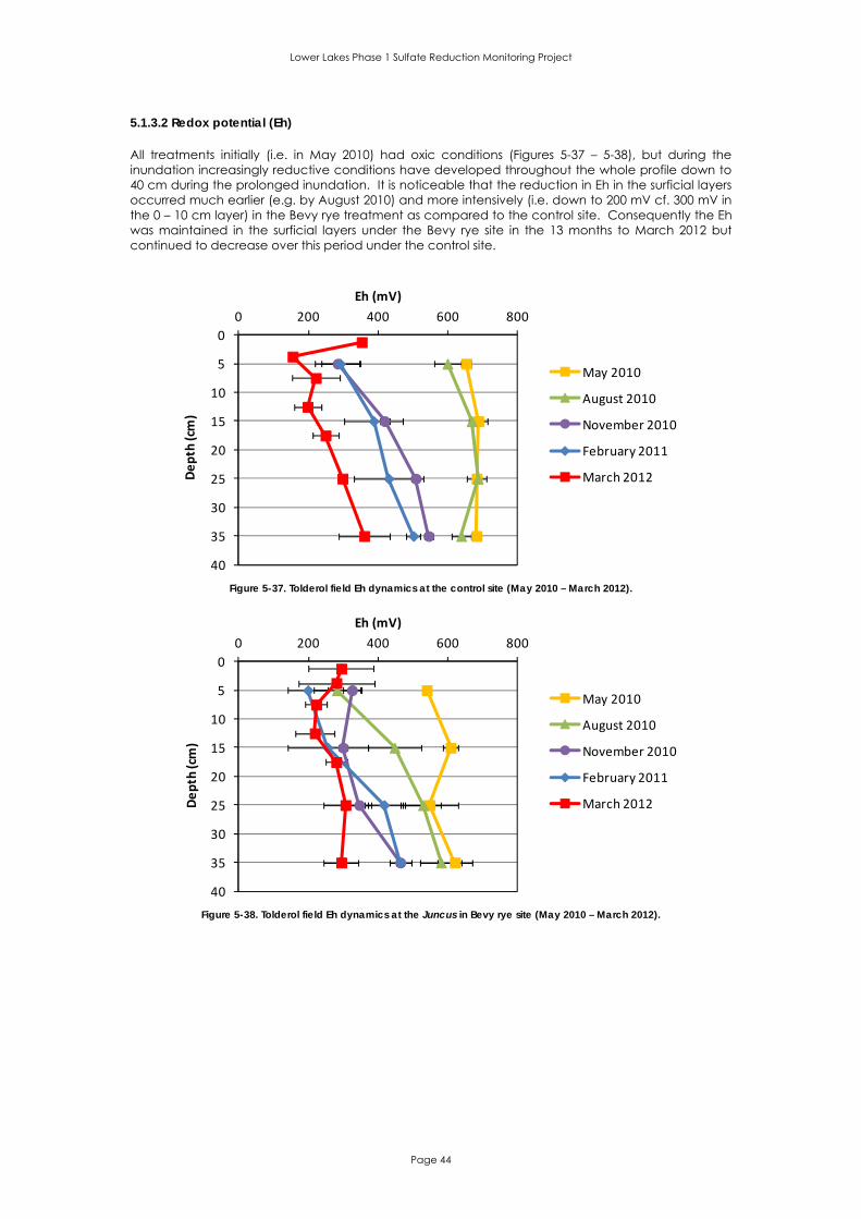
Lower Lakes Phase 1 Sulfate Reduction Monitoring Project
Page 44
5.1.3.2 Redox potential (Eh) All treatments initially (i.e. in May 2010) had oxic conditions (Figures 5-37 – 5-38), but during the inundation increasingly reductive conditions have developed throughout the whole profile down to 40 cm during the prolonged inundation. It is noticeable that the reduction in Eh in the surficial layers occurred much earlier (e.g. by August 2010) and more intensively (i.e. down to 200 mV cf. 300 mV in the 0 – 10 cm layer) in the Bevy rye treatment as compared to the control site. Consequently the Eh was maintained in the surficial layers under the Bevy rye site in the 13 months to March 2012 but continued to decrease over this period under the control site.
0
5
10
15
20
25
30
35
40
0 200 400 600 800
Depth (cm)
Eh (mV)
May 2010
August 2010
November 2010
February 2011
March 2012
Figure 5-37. Tolderol field Eh dynamics at the control site (May 2010 – March 2012).
0
5
10
15
20
25
30
35
40
0 200 400 600 800
Depth (cm)
Eh (mV)
May 2010
August 2010
November 2010
February 2011
March 2012
Figure 5-38. Tolderol field Eh dynamics at the Juncus in Bevy rye site (May 2010 – March 2012).

Lower Lakes Phase 1 Sulfate Reduction Monitoring Project
Page 45
5.1.3.3 Electrical conductivity (EC) As shown in Figures 5-39 – 5-40 the salinity (i.e. EC) decreased appreciably over the 13 months to March 2012 in the sediment layers under both treatments.
0
5
10
15
20
25
30
35
40
0 200 400 600 800
Depth (cm)
EC (µS/cm)
May 2010
August 2010
November 2010
February 2011
March 2012
Figure 5-39. Tolderol EC dynamics at the control site (May 2010 – March 2012).
0
5
10
15
20
25
30
35
40
0 200 400 600 800
Depth (cm)
EC (µS/cm)
May 2010
August 2010
November 2010
February 2011
March 2012
Figure 5-40. Tolderol EC dynamics at the Juncus in Bevy rye site (May 2010 – March 2012).
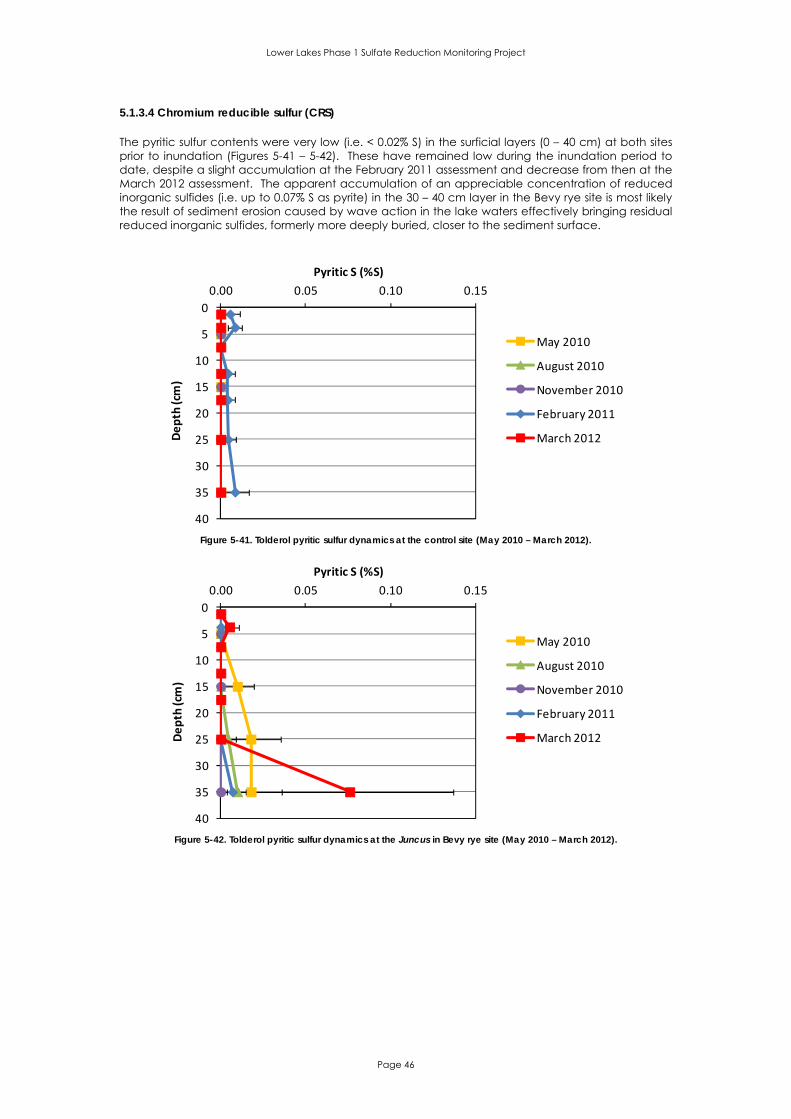
Lower Lakes Phase 1 Sulfate Reduction Monitoring Project
Page 46
5.1.3.4 Chromium reducible sulfur (CRS) The pyritic sulfur contents were very low (i.e. < 0.02% S) in the surficial layers (0 – 40 cm) at both sites prior to inundation (Figures 5-41 – 5-42). These have remained low during the inundation period to date, despite a slight accumulation at the February 2011 assessment and decrease from then at the March 2012 assessment. The apparent accumulation of an appreciable concentration of reduced inorganic sulfides (i.e. up to 0.07% S as pyrite) in the 30 – 40 cm layer in the Bevy rye site is most likely the result of sediment erosion caused by wave action in the lake waters effectively bringing residual reduced inorganic sulfides, formerly more deeply buried, closer to the sediment surface.
0
5
10
15
20
25
30
35
40
0.00 0.05 0.10 0.15
Depth (cm)
Pyritic S (%S)
May 2010
August 2010
November 2010
February 2011
March 2012
Figure 5-41. Tolderol pyritic sulfur dynamics at the control site (May 2010 – March 2012).
0
5
10
15
20
25
30
35
40
0.00 0.05 0.10 0.15
Depth (cm)
Pyritic S (%S)
May 2010
August 2010
November 2010
February 2011
March 2012
Figure 5-42. Tolderol pyritic sulfur dynamics at the Juncus in Bevy rye site (May 2010 – March 2012).
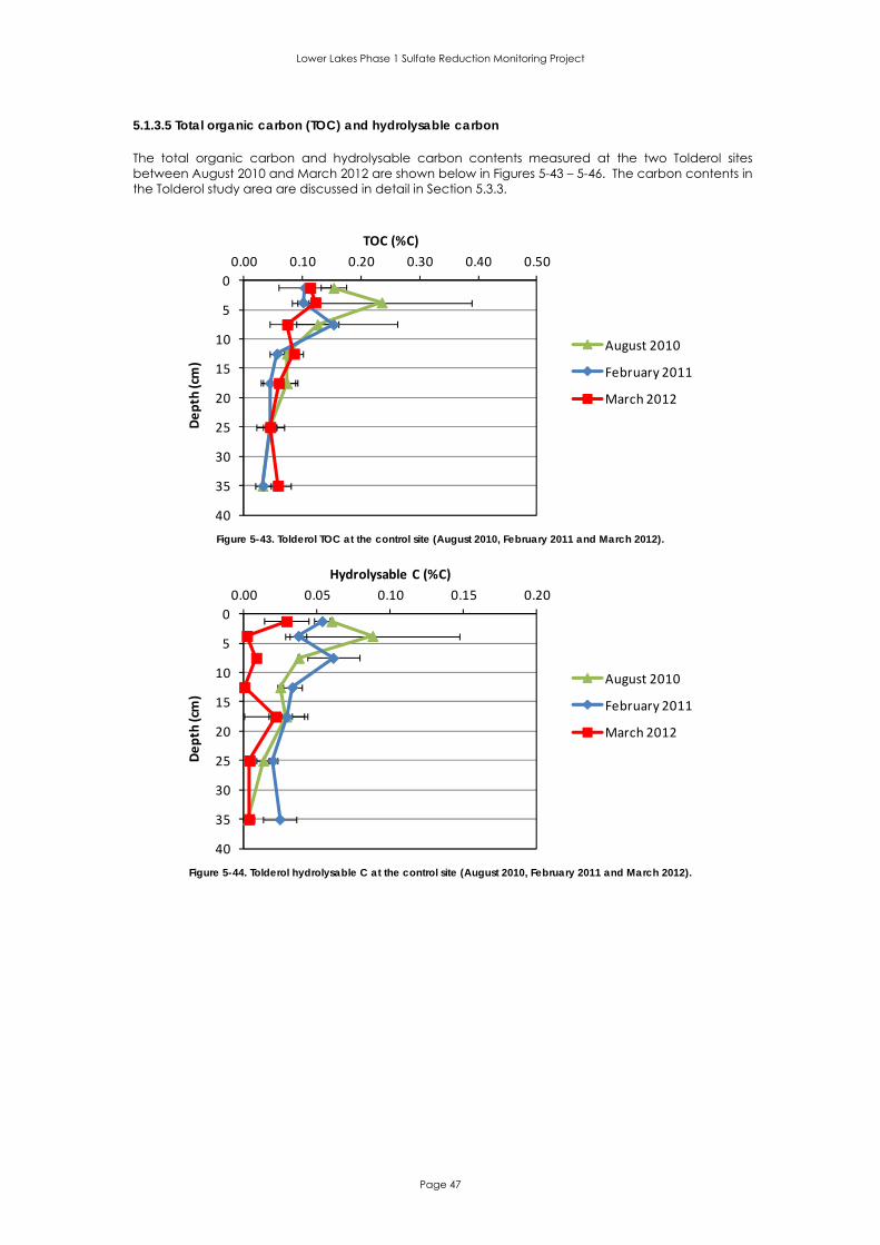
Lower Lakes Phase 1 Sulfate Reduction Monitoring Project
Page 47
5.1.3.5 Total organic carbon (TOC) and hydrolysable carbon The total organic carbon and hydrolysable carbon contents measured at the two Tolderol sites between August 2010 and March 2012 are shown below in Figures 5-43 – 5-46. The carbon contents in the Tolderol study area are discussed in detail in Section 5.3.3.
0
5
10
15
20
25
30
35
40
0.00 0.10 0.20 0.30 0.40 0.50
Depth (cm)
TOC (%C)
August 2010
February 2011
March 2012
Figure 5-43. Tolderol TOC at the control site (August 2010, February 2011 and March 2012).
0
5
10
15
20
25
30
35
40
0.00 0.05 0.10 0.15 0.20
Depth (cm)
Hydrolysable C (%C)
August 2010
February 2011
March 2012
Figure 5-44. Tolderol hydrolysable C at the control site (August 2010, February 2011 and March 2012).
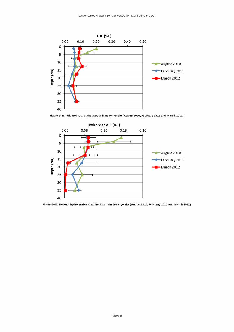
Lower Lakes Phase 1 Sulfate Reduction Monitoring Project
Page 48
0
5
10
15
20
25
30
35
40
0.00 0.10 0.20 0.30 0.40 0.50
Depth (cm)
TOC (%C)
August 2010
February 2011
March 2012
Figure 5-45. Tolderol TOC at the Juncus in Bevy rye site (August 2010, February 2011 and March 2012).
0
5
10
15
20
25
30
35
40
0.00 0.05 0.10 0.15 0.20
Depth (cm)
Hydrolysable C (%C)
August 2010
February 2011
March 2012
Figure 5-46. Tolderol hydrolysable C at the Juncus in Bevy rye site (August 2010, February 2011 and March 2012).
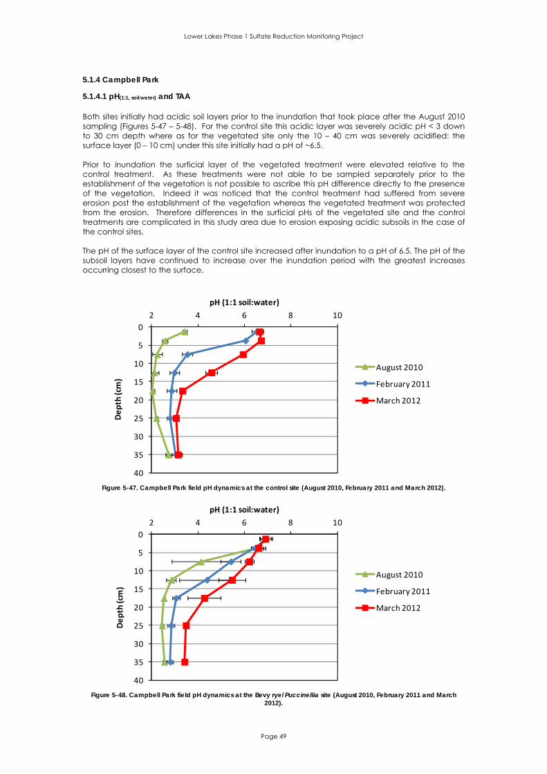
Lower Lakes Phase 1 Sulfate Reduction Monitoring Project
Page 49
5.1.4 Campbell Park
5.1.4.1 pH(1:1, soil:water) and TAA Both sites initially had acidic soil layers prior to the inundation that took place after the August 2010 sampling (Figures 5-47 – 5-48). For the control site this acidic layer was severely acidic pH < 3 down to 30 cm depth where as for the vegetated site only the 10 – 40 cm was severely acidified: the surface layer (0 – 10 cm) under this site initially had a pH of ~6.5. Prior to inundation the surficial layer of the vegetated treatment were elevated relative to the control treatment. As these treatments were not able to be sampled separately prior to the establishment of the vegetation is not possible to ascribe this pH difference directly to the presence of the vegetation. Indeed it was noticed that the control treatment had suffered from severe erosion post the establishment of the vegetation whereas the vegetated treatment was protected from the erosion. Therefore differences in the surficial pHs of the vegetated site and the control treatments are complicated in this study area due to erosion exposing acidic subsoils in the case of the control sites. The pH of the surface layer of the control site increased after inundation to a pH of 6.5. The pH of the subsoil layers have continued to increase over the inundation period with the greatest increases occurring closest to the surface.
0
5
10
15
20
25
30
35
40
2 4 6 8 10
Depth (cm)
pH (1:1 soil:water)
August 2010
February 2011
March 2012
Figure 5-47. Campbell Park field pH dynamics at the control site (August 2010, February 2011 and March 2012).
0
5
10
15
20
25
30
35
40
2 4 6 8 10
Depth (cm)
pH (1:1 soil:water)
August 2010
February 2011
March 2012
Figure 5-48. Campbell Park field pH dynamics at the Bevy rye/Puccinellia site (August 2010, February 2011 and March
2012).

Lower Lakes Phase 1 Sulfate Reduction Monitoring Project
Page 50
The TAAs (Figures 5-49 – 5-50) were all low in the surface soil layers (i.e. < 18 mol H+ t-1) but increased up to 35 mol H+ t-1 in the 30 - 40 cm layers of each site both prior to and during inundation. This is the zone that contains appreciable quantities of jarosite and other iron oxides and this may account for the much higher TAAs found at Campbell Park compared to the other experimental locations in this study.
0
5
10
15
20
25
30
35
40
0 20 40 60
Depth (cm)
TAA (mol H+/t)
August 2010
November 2010
February 2011
March 2012
Figure 5-49. Campbell Park TAA dynamics at the control site (August 2010 – March 2012).
0
5
10
15
20
25
30
35
40
0 20 40 60
Depth (cm)
TAA (mol H+/t)
August 2010
November 2010
February 2011
March 2012
Figure 5-50. Campbell Park TAA dynamics at the Bevy rye/Puccinellia site (August 2010 – March 2012).
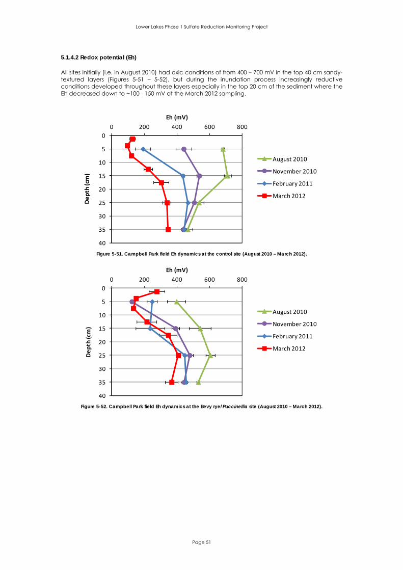
Lower Lakes Phase 1 Sulfate Reduction Monitoring Project
Page 51
5.1.4.2 Redox potential (Eh) All sites initially (i.e. in August 2010) had oxic conditions of from 400 – 700 mV in the top 40 cm sandy-textured layers (Figures 5-51 – 5-52), but during the inundation process increasingly reductive conditions developed throughout these layers especially in the top 20 cm of the sediment where the Eh decreased down to ~100 - 150 mV at the March 2012 sampling.
0
5
10
15
20
25
30
35
40
0 200 400 600 800
Depth (cm)
Eh (mV)
August 2010
November 2010
February 2011
March 2012
Figure 5-51. Campbell Park field Eh dynamics at the control site (August 2010 – March 2012).
0
5
10
15
20
25
30
35
40
0 200 400 600 800
Depth (cm)
Eh (mV)
August 2010
November 2010
February 2011
March 2012
Figure 5-52. Campbell Park field Eh dynamics at the Bevy rye/Puccinellia site (August 2010 – March 2012).
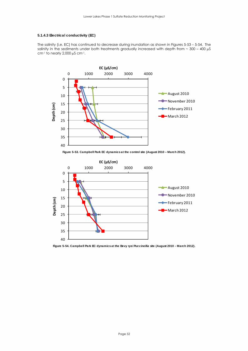
Lower Lakes Phase 1 Sulfate Reduction Monitoring Project
Page 52
5.1.4.3 Electrical conductivity (EC) The salinity (i.e. EC) has continued to decrease during inundation as shown in Figures 5-53 – 5-54. The salinity in the sediments under both treatments gradually increased with depth from ~ 300 – 400 S cm-1 to nearly 2,000 S cm-1.
0
5
10
15
20
25
30
35
40
0 1000 2000 3000 4000
Depth (cm)
EC (µS/cm)
August 2010
November 2010
February 2011
March 2012
Figure 5-53. Campbell Park EC dynamics at the control site (August 2010 – March 2012).
0
5
10
15
20
25
30
35
40
0 1000 2000 3000 4000
Depth (cm)
EC (µS/cm)
August 2010
November 2010
February 2011
March 2012
Figure 5-54. Campbell Park EC dynamics at the Bevy rye/Puccinellia site (August 2010 – March 2012).

Lower Lakes Phase 1 Sulfate Reduction Monitoring Project
Page 53
5.1.4.4 Chromium reducible sulfur (CRS) The pyritic sulfur contents were low (i.e. < 0.02% S) in the surficial layers (0 – 20 cm) at both sites (Figures 5-55 – 5-56) prior to inundation. The apparent accumulation of an appreciable concentration of reduced inorganic sulfides (i.e. up to 0.70% S as pyrite) in the 30 – 40 cm layer in the control site is most likely the result of sediment erosion caused by wave action in the lake waters effectively bringing residual reduced inorganic sulfides, formerly more deeply buried, closer to the sediment surface. There was no evidence of the accumulation of reduced inorganic sulfides in the surficial sediments after inundation to date.
0
5
10
15
20
25
30
35
40
0.00 0.20 0.40 0.60 0.80 1.00
Depth (cm)
Pyritic S (%S)
August 2010
November 2010
February 2011
March 2012
Figure 5-55. Campbell Park pyritic sulfur dynamics at the control site (August 2010 – March 2012).
0
5
10
15
20
25
30
35
40
0.00 0.20 0.40 0.60 0.80 1.00
Depth (cm)
Pyritic S (%S)
August 2010
November 2010
February 2011
March 2012
Figure 5-56. Campbell Park pyritic sulfur dynamics at the Bevy rye/Puccinellia site (August 2010 – March 2012).

Lower Lakes Phase 1 Sulfate Reduction Monitoring Project
Page 54
5.1.4.5 Total organic carbon (TOC) and hydrolysable carbon The total organic carbon and hydrolysable carbon contents measured at the two Campbell Park sites between August 2010 and March 2012 are shown below in Figures 5-57 – 5-60. The carbon contents in the Campbell Park study area are discussed in detail in Section 5.3.4.
0
5
10
15
20
25
30
35
40
0.00 0.50 1.00 1.50
Depth (cm)
TOC (%C)
August 2010
February 2011
March 2012
Figure 5-57. Campbell Park field TOC at the control site (August 2010, February 2011 and March 2012).
0
5
10
15
20
25
30
35
40
0.00 0.10 0.20 0.30 0.40
Depth (cm)
Hydrolysable C (%C)
August 2010
February 2011
March 2012
Figure 5-58. Campbell Park field hydrolysable C at the control site (August 2010, February 2011 and March 2012).

Lower Lakes Phase 1 Sulfate Reduction Monitoring Project
Page 55
0
5
10
15
20
25
30
35
40
0.00 0.50 1.00 1.50
Depth (cm)
TOC (%C)
August 2010
February 2011
March 2012
Figure 5-59. Campbell Park field TOC at the Bevy rye/Puccinellia site (August 2010, February 2011 and March 2012).
0
5
10
15
20
25
30
35
40
0.00 0.10 0.20 0.30 0.40
Depth (cm)
Hydrolysable C (%C)
August 2010
February 2011
March 2012
Figure 5-60. Campbell Park field hydrolysable C in at the Bevy rye/Puccinellia site
(August 2010, February 2011 and March 2012).
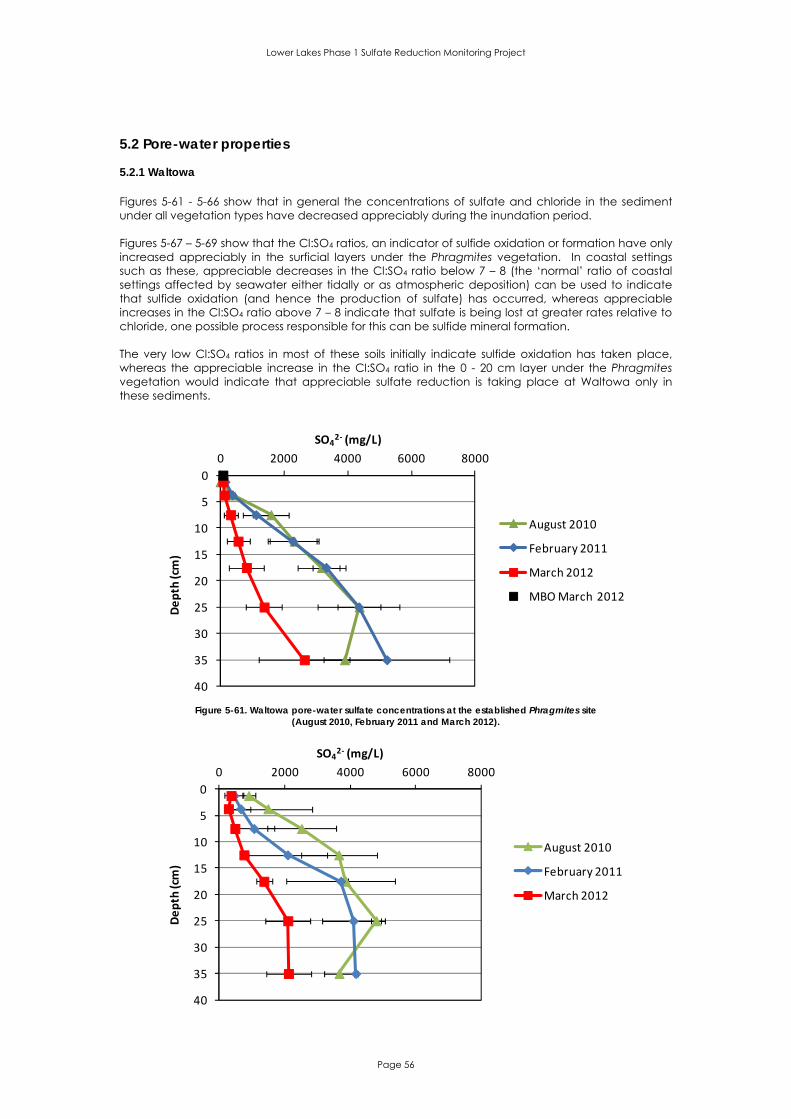
Lower Lakes Phase 1 Sulfate Reduction Monitoring Project
Page 56
5.2 Pore-water properties
5.2.1 Waltowa Figures 5-61 - 5-66 show that in general the concentrations of sulfate and chloride in the sediment under all vegetation types have decreased appreciably during the inundation period. Figures 5-67 – 5-69 show that the Cl:SO4 ratios, an indicator of sulfide oxidation or formation have only increased appreciably in the surficial layers under the Phragmites vegetation. In coastal settings such as these, appreciable decreases in the Cl:SO4 ratio below 7 – 8 (the ‘normal’ ratio of coastal settings affected by seawater either tidally or as atmospheric deposition) can be used to indicate that sulfide oxidation (and hence the production of sulfate) has occurred, whereas appreciable increases in the Cl:SO4 ratio above 7 – 8 indicate that sulfate is being lost at greater rates relative to chloride, one possible process responsible for this can be sulfide mineral formation. The very low Cl:SO4 ratios in most of these soils initially indicate sulfide oxidation has taken place, whereas the appreciable increase in the Cl:SO4 ratio in the 0 - 20 cm layer under the Phragmites vegetation would indicate that appreciable sulfate reduction is taking place at Waltowa only in these sediments.
0
5
10
15
20
25
30
35
40
0 2000 4000 6000 8000
Depth (cm)
SO42‐ (mg/L)
August 2010
February 2011
March 2012
MBO March 2012
Figure 5-61. Waltowa pore-water sulfate concentrations at the established Phragmites site
(August 2010, February 2011 and March 2012).
0
5
10
15
20
25
30
35
40
0 2000 4000 6000 8000
Depth (cm)
SO42‐ (mg/L)
August 2010
February 2011
March 2012

Lower Lakes Phase 1 Sulfate Reduction Monitoring Project
Page 57
Figure 5-62. Waltowa pore-water sulfate concentrations at the established Cotula site (August 2010, February 2011 and March 2012).
0
5
10
15
20
25
30
35
40
0 2000 4000 6000 8000Depth (cm)
SO42‐ (mg/L)
August 2010
February 2011
March 2012
Figure 5-63. Waltowa pore-water sulfate concentrations at the established Juncus site
(August 2010, February 2011 and March 2012).
0
5
10
15
20
25
30
35
40
0 5000 10000 15000
Depth (cm)
Cl (mg/L)
August 2010
February 2011
March 2012
MBO March 2012
Figure 5-64. Waltowa pore-water chloride concentrations at the established Phragmites site
(August 2010, February 2011 and March 2012).
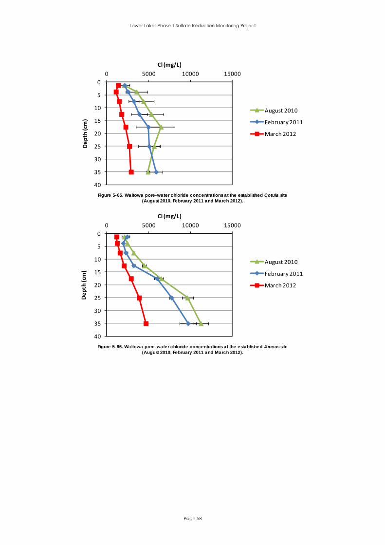
Lower Lakes Phase 1 Sulfate Reduction Monitoring Project
Page 58
0
5
10
15
20
25
30
35
40
0 5000 10000 15000
Depth (cm)
Cl (mg/L)
August 2010
February 2011
March 2012
Figure 5-65. Waltowa pore-water chloride concentrations at the established Cotula site
(August 2010, February 2011 and March 2012).
0
5
10
15
20
25
30
35
40
0 5000 10000 15000
Depth (cm)
Cl (mg/L)
August 2010
February 2011
March 2012
Figure 5-66. Waltowa pore-water chloride concentrations at the established Juncus site
(August 2010, February 2011 and March 2012).

Lower Lakes Phase 1 Sulfate Reduction Monitoring Project
Page 59
0
5
10
15
20
25
30
35
40
0 10 20 30 40
Depth (cm)
Cl:SO4 ratio
August 2010
February 2011
March 2012
MBO March 2012
Figure 5-67. Waltowa pore-water chloride/sulfate ratios at the established Phragmites site
(August 2010, February 2011 and March 2012).
0
5
10
15
20
25
30
35
40
0 5 10 15 20
Depth (cm)
Cl:SO4 ratio
August 2010
February 2011
March 2012
Figure 5-68. Waltowa pore-water chloride/sulfate ratios at the established Cotula site
(August 2010, February 2011 and March 2012).
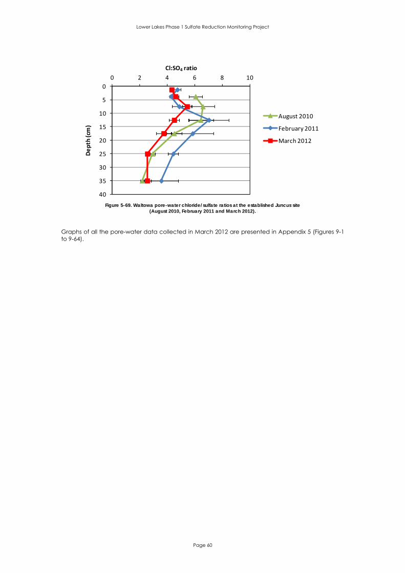
Lower Lakes Phase 1 Sulfate Reduction Monitoring Project
Page 60
0
5
10
15
20
25
30
35
40
0 2 4 6 8 10
Depth (cm)
Cl:SO4 ratio
August 2010
February 2011
March 2012
Figure 5-69. Waltowa pore-water chloride/sulfate ratios at the established Juncus site
(August 2010, February 2011 and March 2012). Graphs of all the pore-water data collected in March 2012 are presented in Appendix 5 (Figures 9-1 to 9-64).
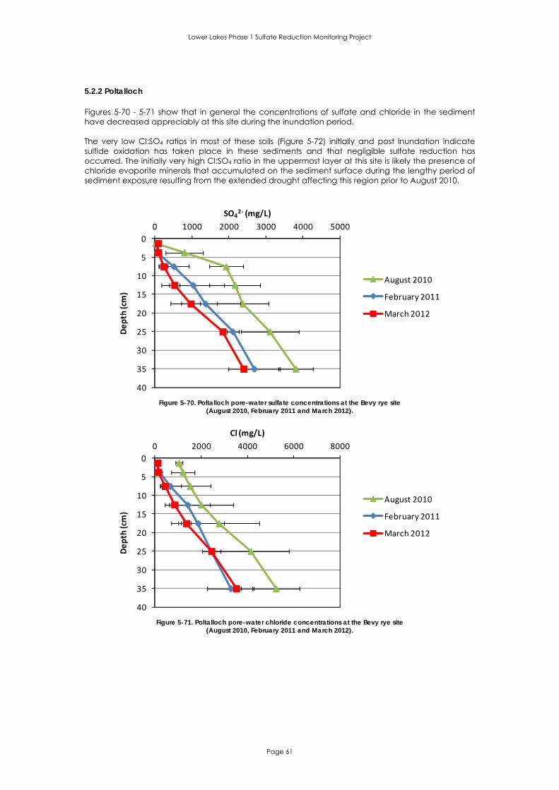
Lower Lakes Phase 1 Sulfate Reduction Monitoring Project
Page 61
5.2.2 Poltalloch Figures 5-70 - 5-71 show that in general the concentrations of sulfate and chloride in the sediment have decreased appreciably at this site during the inundation period. The very low Cl:SO4 ratios in most of these soils (Figure 5-72) initially and post inundation indicate sulfide oxidation has taken place in these sediments and that negligible sulfate reduction has occurred. The initially very high Cl:SO4 ratio in the uppermost layer at this site is likely the presence of chloride evaporite minerals that accumulated on the sediment surface during the lengthy period of sediment exposure resulting from the extended drought affecting this region prior to August 2010.
0
5
10
15
20
25
30
35
40
0 1000 2000 3000 4000 5000
Depth (cm)
SO42‐ (mg/L)
August 2010
February 2011
March 2012
Figure 5-70. Poltalloch pore-water sulfate concentrations at the Bevy rye site
(August 2010, February 2011 and March 2012).
0
5
10
15
20
25
30
35
40
0 2000 4000 6000 8000
Depth (cm)
Cl (mg/L)
August 2010
February 2011
March 2012
Figure 5-71. Poltalloch pore-water chloride concentrations at the Bevy rye site
(August 2010, February 2011 and March 2012).
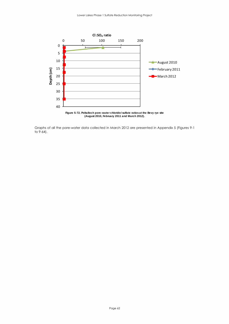
Lower Lakes Phase 1 Sulfate Reduction Monitoring Project
Page 62
0
5
10
15
20
25
30
35
40
0 50 100 150 200
Depth (cm)
Cl :SO4 ratio
August 2010
February 2011
March 2012
Figure 5-72. Poltalloch pore-water chloride/sulfate ratios at the Bevy rye site
(August 2010, February 2011 and March 2012). Graphs of all the pore-water data collected in March 2012 are presented in Appendix 5 (Figures 9-1 to 9-64).

Lower Lakes Phase 1 Sulfate Reduction Monitoring Project
Page 63
5.2.3 Tolderol Figures 5-73 - 5-76 show that in general the concentrations of sulfate and chloride in the sediment have decreased appreciably at this study area during the inundation period. The very low Cl:SO4 ratios in most of these soils (Figure 5-77 – 5-78) initially and post inundation indicate sulfide oxidation has taken place in these sediments and that negligible sulfate reduction has occurred. The initially high Cl:SO4 ratio in the uppermost layer at the Bevy Rye site is likely the presence of chloride evaporite minerals that accumulated on the sediment surface during the lengthy period of sediment exposure resulting from the extended drought affecting this region prior to August 2010.
0
5
10
15
20
25
30
35
40
0 1000 2000 3000 4000
Depth (cm)
SO42‐ (mg/L)
August 2010
February 2011
March 2012
Figure 5-73. Tolderol pore-water sulfate concentrations at the control site
(August 2010, February 2011 and March 2012).
0
5
10
15
20
25
30
35
40
0 1000 2000 3000 4000
Depth (cm)
SO42‐ (mg/L)
August 2010
February 2011
March 2012
Figure 5-74. Tolderol pore-water sulfate concentrations at the Juncus in Bevy rye site
(August 2010, February 2011 and March 2012).
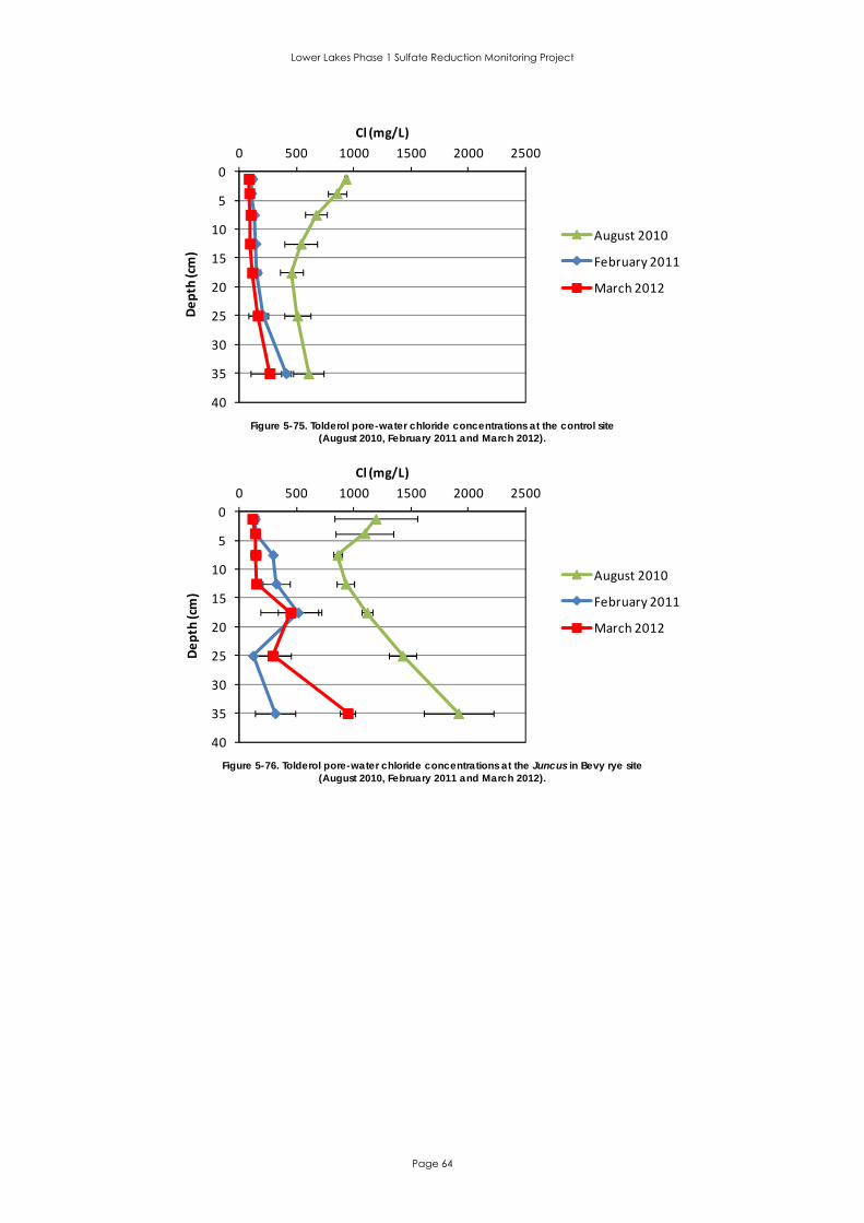
Lower Lakes Phase 1 Sulfate Reduction Monitoring Project
Page 64
0
5
10
15
20
25
30
35
40
0 500 1000 1500 2000 2500
Depth (cm)
Cl (mg/L)
August 2010
February 2011
March 2012
Figure 5-75. Tolderol pore-water chloride concentrations at the control site
(August 2010, February 2011 and March 2012).
0
5
10
15
20
25
30
35
40
0 500 1000 1500 2000 2500
Depth (cm)
Cl (mg/L)
August 2010
February 2011
March 2012
Figure 5-76. Tolderol pore-water chloride concentrations at the Juncus in Bevy rye site
(August 2010, February 2011 and March 2012).
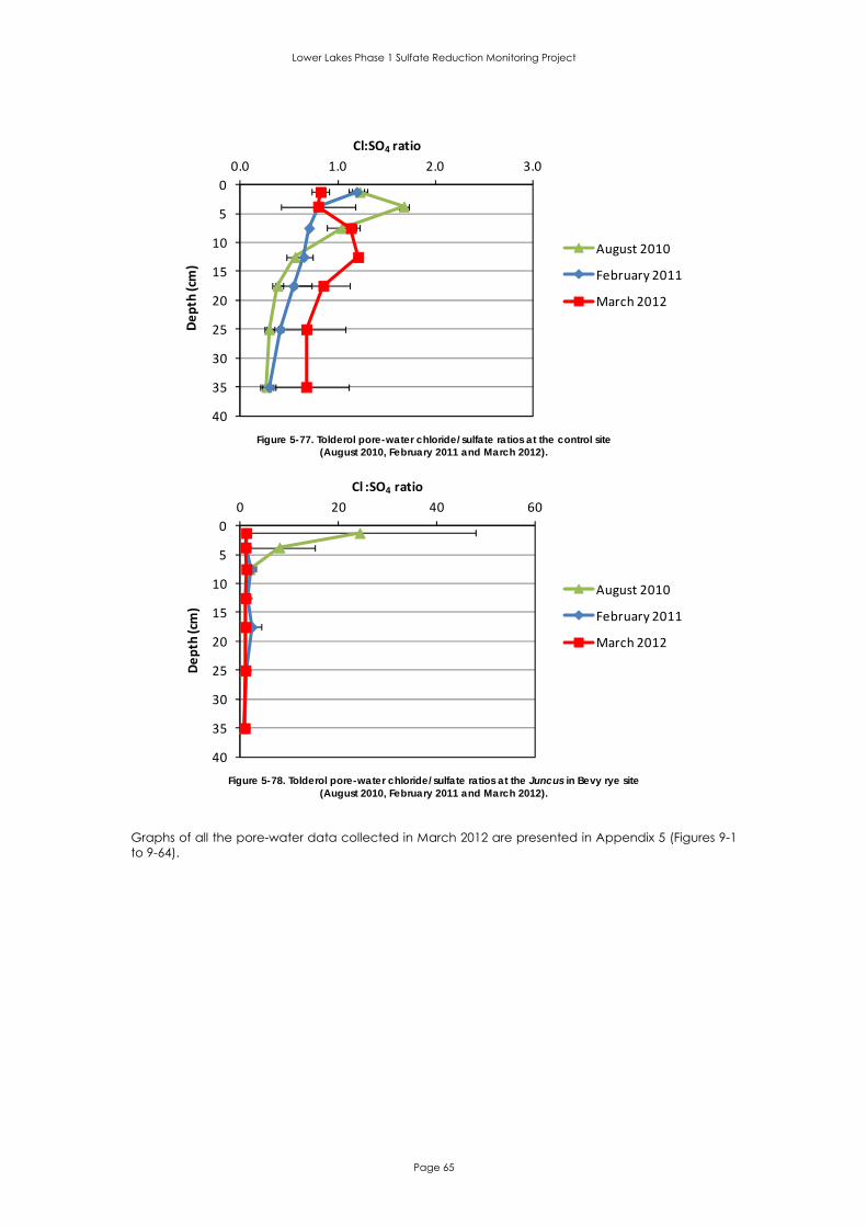
Lower Lakes Phase 1 Sulfate Reduction Monitoring Project
Page 65
0
5
10
15
20
25
30
35
40
0.0 1.0 2.0 3.0
Depth (cm)
Cl:SO4 ratio
August 2010
February 2011
March 2012
Figure 5-77. Tolderol pore-water chloride/sulfate ratios at the control site
(August 2010, February 2011 and March 2012).
0
5
10
15
20
25
30
35
40
0 20 40 60
Depth (cm)
Cl :SO4 ratio
August 2010
February 2011
March 2012
Figure 5-78. Tolderol pore-water chloride/sulfate ratios at the Juncus in Bevy rye site
(August 2010, February 2011 and March 2012). Graphs of all the pore-water data collected in March 2012 are presented in Appendix 5 (Figures 9-1 to 9-64).

Lower Lakes Phase 1 Sulfate Reduction Monitoring Project
Page 66
5.2.4 Campbell Park Figures 5-79 - 5-82 show that in general the concentrations of sulfate and chloride in the sediment have decreased appreciably at this study area during the inundation period. The very low Cl:SO4 ratios in most of these soils (Figure 5-83 – 5-84) initially and post inundation indicate sulfide oxidation has taken place in these sediments. The appreciable increase in the Cl:SO4 ratios in the uppermost sediment layers at both sites indicates that sulfate reduction has occurred in both sites since inundation.
0
5
10
15
20
25
30
35
40
0 2000 4000 6000 8000 10000
Depth (cm)
SO42‐ (mg/L)
August 2010
February 2011
March 2012
Figure 5-79. Campbell Park pore-water sulfate concentrations at the control site
(August 2010, February 2011 and March 2012).
0
5
10
15
20
25
30
35
40
0 2000 4000 6000 8000 10000
Depth (cm)
SO42‐ (mg/L)
August 2010
February 2011
March 2012
Figure 5-80. Campbell Park pore-water sulfate concentrations at the Bevy rye/Puccinellia site
(August 2010, February 2011 and March 2012).

Lower Lakes Phase 1 Sulfate Reduction Monitoring Project
Page 67
0
5
10
15
20
25
30
35
40
0 2000 4000 6000 8000
Depth (cm)
Cl (mg/L)
August 2010
February 2011
March 2012
Figure 5-81. Campbell Park pore-water chloride concentrations at the control site
(August 2010, February 2011 and March 2012).
0
5
10
15
20
25
30
35
40
0 2000 4000 6000 8000
Depth (cm)
Cl (mg/L)
August 2010
February 2011
March 2012
Figure 5-82. Campbell Park pore-water chloride concentrations at the Bevy rye/Puccinellia site
(August 2010, February 2011 and March 2012).
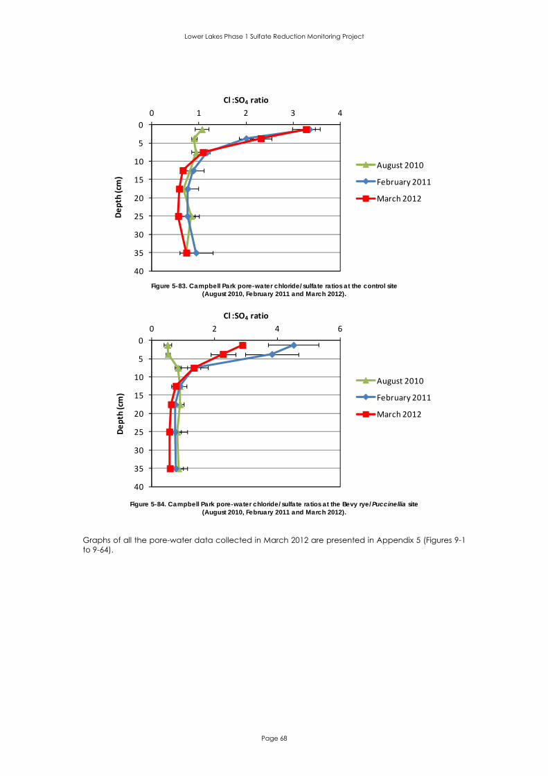
Lower Lakes Phase 1 Sulfate Reduction Monitoring Project
Page 68
0
5
10
15
20
25
30
35
40
0 1 2 3 4Depth (cm)
Cl :SO4 ratio
August 2010
February 2011
March 2012
Figure 5-83. Campbell Park pore-water chloride/sulfate ratios at the control site
(August 2010, February 2011 and March 2012).
0
5
10
15
20
25
30
35
40
0 2 4 6
Depth (cm)
Cl :SO4 ratio
August 2010
February 2011
March 2012
Figure 5-84. Campbell Park pore-water chloride/sulfate ratios at the Bevy rye/Puccinellia site
(August 2010, February 2011 and March 2012). Graphs of all the pore-water data collected in March 2012 are presented in Appendix 5 (Figures 9-1 to 9-64).

Lower Lakes Phase 1 Sulfate Reduction Monitoring Project
Page 69
5.3 Sulfate reduction rates
5.3.1 Waltowa sulfate reduction rates The sulfate reduction rates measured at the three Waltowa sites between August 2010 and March 2012 are shown below in Figures 5-85, 5-86 and 5-87.
0
5
10
15
20
25
30
35
40
0 200 400 600 800 1000
Depth (cm)
Total SRR (nmol/g/day)
August 2010
February 2011
March 2012
Figure 5-85. Waltowa sulfate reduction rates (nmol/g/day) at the established Phragmites site
(August 2010, February 2011 and March 2012).
0
5
10
15
20
25
30
35
40
0 20 40 60 80
Depth (cm)
Total SRR (nmol/g/day)
August 2010
February 2011
March 2012
Figure 5-86. Waltowa sulfate reduction rates (nmol/g/day) at the established Cotula site
(August 2010, February 2011 and March 2012).

Lower Lakes Phase 1 Sulfate Reduction Monitoring Project
Page 70
0
5
10
15
20
25
30
35
40
0 5 10 15 20 25
Depth (cm)
Total SRR (nmol/g/day)
August 2010
February 2011
March 2012
Figure 5-87. Waltowa sulfate reduction rates (nmol/g/day) at the established Juncus site in
(August 2010, February 2011 and March 2012). Figures 5-85 – 5-87 clearly show:
Sulfate reduction was mainly limited to the 0 - 20 cm layers of the sediment at each treatment site.
Sulfate reduction in the near inundating conditions in the August 2010 assessment only allowed limited sulfate reduction and only in the Phragmites treatment and only at relatively low rates (i.e. ~10 nmol g-1 day-1).
6 months of inundation (February 2011 assessment) allowed appreciable sulfate reduction to occur in the 0 - 2.5 cm layer of all treatments, but with much higher rates in the Phragmites site (i.e. 170 nmol g-1 day-1) than in the Cotula treatment (32 nmol g-1 day-1) or the Juncus treatment (~15 nmol g-1 day-1).
19 months of months of inundation (March 2012 assessment) allowed sulfate reduction to be further enhanced at the Phragmites site at rates of up to 700 nmol g-1 day-1 and within the 0 - 20 cm layer (Figure 5-85).
In contrast 19 months of months of inundation resulted in further restricted sulfate reduction in the sediments under both the Cotula and Juncus treatments (~15 nmol g-1 day-1) (Figures 5-86 – 5-87).
Figure 5-88 shows the strong effect of the Phragmites vegetation on the rates of sulfate reduction in the sediments after 19 months of inundation.
0
5
10
15
20
25
30
35
40
0 200 400 600 800 1000
Depth (cm)
Total SRR (nmol/g/day)
Phragmites
Cotula
Juncus
Figure 5-88. Waltowa sulfate reduction rates (nmol/g/day) at the established Phragmites, Cotula and Juncus
sites in March 2012.
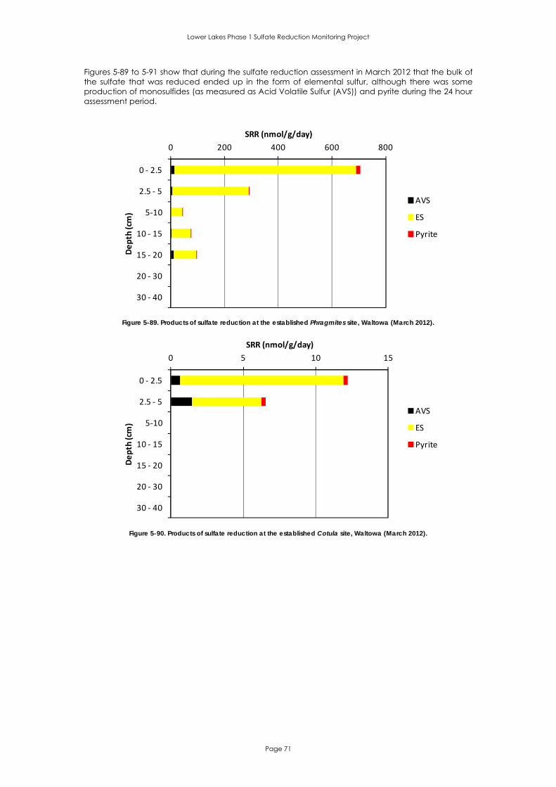
Lower Lakes Phase 1 Sulfate Reduction Monitoring Project
Page 71
Figures 5-89 to 5-91 show that during the sulfate reduction assessment in March 2012 that the bulk of the sulfate that was reduced ended up in the form of elemental sulfur, although there was some production of monosulfides (as measured as Acid Volatile Sulfur (AVS)) and pyrite during the 24 hour assessment period.
0 200 400 600 800
0 ‐ 2.5
2.5 ‐ 5
5‐10
10 ‐ 15
15 ‐ 20
20 ‐ 30
30 ‐ 40
SRR (nmol/g/day)Depth (cm)
AVS
ES
Pyrite
Figure 5-89. Products of sulfate reduction at the established Phragmites site, Waltowa (March 2012).
0 5 10 15
0 ‐ 2.5
2.5 ‐ 5
5‐10
10 ‐ 15
15 ‐ 20
20 ‐ 30
30 ‐ 40
SRR (nmol/g/day)
Depth (cm)
AVS
ES
Pyrite
Figure 5-90. Products of sulfate reduction at the established Cotula site, Waltowa (March 2012).
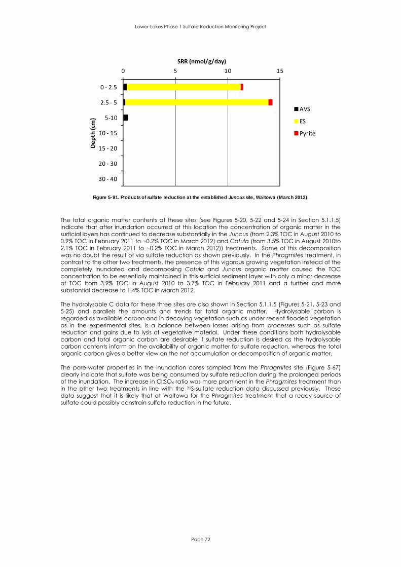
Lower Lakes Phase 1 Sulfate Reduction Monitoring Project
Page 72
0 5 10 15
0 ‐ 2.5
2.5 ‐ 5
5‐10
10 ‐ 15
15 ‐ 20
20 ‐ 30
30 ‐ 40
SRR (nmol/g/day)
Depth (cm)
AVS
ES
Pyrite
Figure 5-91. Products of sulfate reduction at the established Juncus site, Waltowa (March 2012).
The total organic matter contents at these sites (see Figures 5-20, 5-22 and 5-24 in Section 5.1.1.5) indicate that after inundation occurred at this location the concentration of organic matter in the surficial layers has continued to decrease substantially in the Juncus (from 2.3% TOC in August 2010 to 0.9% TOC in February 2011 to ~0.2% TOC in March 2012) and Cotula (from 3.5% TOC in August 2010to 2.1% TOC in February 2011 to ~0.2% TOC in March 2012)) treatments. Some of this decomposition was no doubt the result of via sulfate reduction as shown previously. In the Phragmites treatment, in contrast to the other two treatments, the presence of this vigorous growing vegetation instead of the completely inundated and decomposing Cotula and Juncus organic matter caused the TOC concentration to be essentially maintained in this surficial sediment layer with only a minor decrease of TOC from 3.9% TOC in August 2010 to 3.7% TOC in February 2011 and a further and more substantial decrease to 1.4% TOC in March 2012. The hydrolysable C data for these three sites are also shown in Section 5.1.1.5 (Figures 5-21, 5-23 and 5-25) and parallels the amounts and trends for total organic matter. Hydrolysable carbon is regarded as available carbon and in decaying vegetation such as under recent flooded vegetation as in the experimental sites, is a balance between losses arising from processes such as sulfate reduction and gains due to lysis of vegetative material. Under these conditions both hydrolysable carbon and total organic carbon are desirable if sulfate reduction is desired as the hydrolysable carbon contents inform on the availability of organic matter for sulfate reduction, whereas the total organic carbon gives a better view on the net accumulation or decomposition of organic matter. The pore-water properties in the inundation cores sampled from the Phragmites site (Figure 5-67) clearly indicate that sulfate was being consumed by sulfate reduction during the prolonged periods of the inundation. The increase in Cl:SO4 ratio was more prominent in the Phragmites treatment than in the other two treatments in line with the 35S-sulfate reduction data discussed previously. These data suggest that it is likely that at Waltowa for the Phragmites treatment that a ready source of sulfate could possibly constrain sulfate reduction in the future.

Lower Lakes Phase 1 Sulfate Reduction Monitoring Project
Page 73
5.3.2 Sulfate reduction rates at Poltalloch The sulfate reduction rates measured at the Poltalloch site between August 2010 and March 2012 are shown below in Figure 5-92.
0
5
10
15
20
25
30
35
40
0.00 1.00 2.00 3.00 4.00 5.00
Depth (cm)
Total SRR (nmol/g/day)
August 2010
February 2011
March 2012
Figure 5-92. Poltalloch sulfate reduction rates (nmol/g/day) at the Bevy rye only site
(August 2010, February 2011 and March 2012). Figure 5-92 clearly show:
Sulfate reduction was negligible during the March 2012 assessment period and declined considerably from even the very low rates of sulfate reduction observed during the two earlier assessment periods.
The product of the sulfate reduction during the March 2012 assessment period was a very low rate of AVS production in the 0 – 2.5 cm layer
Figure 5-93 show that during the sulfate reduction period in March 2012 that the small amount of sulfate that was reduced ended up in the form of monosulfides (as measured as Acid Volatile Sulfur (AVS)).
0.00 0.01 0.02 0.03 0.04 0.05
0 ‐ 2.5
2.5 ‐ 5
5‐10
10 ‐ 15
15 ‐ 20
20 ‐ 30
30 ‐ 40
SRR (nmol/g/day)
Depth (cm)
AVS
ES
Pyrite
Figure 5-93. Products of sulfate reduction at the Bevy rye only site, Poltalloch (March 2012).

Lower Lakes Phase 1 Sulfate Reduction Monitoring Project
Page 74
The total organic matter contents at this site (see Figures 5-31 and 5-32 in Section 5.1.2.5) indicate that after inundation occurred at this location the concentration of organic matter in the surficial layer decreased from a relatively low value of ~ 0.20% TOC and ~ 0.10% hydrolysable carbon in August, to 0.02 – 0.10 % TOC comprised mainly of hydrolysable carbon after prolonged inundation. Some of this organic matter decomposition was likely the result of sulfate reduction occurring in the first 6 months of inundation as shown previously. It is most probable that the observed substantial decreases in sulfate reduction rates in February 2011 at this site compared to those observed in August 2010 are due to the near exhaustion of initially low organic matter content in these sediments, as a result of sulfate reduction since inundation in August 2010. In March 2012 the content of organic matter remained very low and apparently acted as the constraint on sulfate reduction at this site.
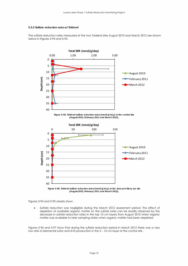
Lower Lakes Phase 1 Sulfate Reduction Monitoring Project
Page 75
5.3.3 Sulfate reduction rates at Tolderol The sulfate reduction rates measured at the two Tolderol sites August 2010 and March 2012 are shown below in Figures 5-94 and 5-95.
0
5
10
15
20
25
30
35
40
0.00 1.00 2.00 3.00
Depth (cm)
Total SRR (nmol/g/day)
August 2010
February 2011
March 2012
Figure 5-94. Tolderol sulfate reduction rates (nmol/g/day) at the control site
(August 2010, February 2011 and March 2012).
0
5
10
15
20
25
30
35
40
0 50 100 150
Depth (cm)
Total SRR (nmol/g/day)
August 2010
February 2011
March 2012
Figure 5-95. Tolderol sulfate reduction rates (nmol/g/day) at the Juncus in Bevy rye site
(August 2010, February 2011 and March 2012). Figures 5-94 and 5-95 clearly show:
Sulfate reduction was negligible during the March 2012 assessment period. The effect of depletion of available organic matter on the sulfate rates can be readily observed by the decrease in sulfate reduction rates in the top 10 cm layers from August 2010 when organic matter was available to later sampling dates when organic matter had been depleted.
Figures 5-96 and 5-97 show that during the sulfate reduction period in March 2012 there was a very low rate of elemental sulfur and AVS production in the 5 – 10 cm layer at the control site.
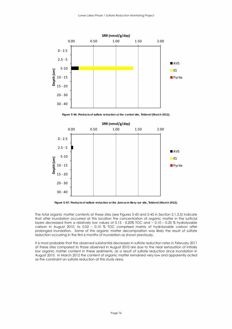
Lower Lakes Phase 1 Sulfate Reduction Monitoring Project
Page 76
0.00 0.50 1.00 1.50 2.00
0 ‐ 2.5
2.5 ‐ 5
5‐10
10 ‐ 15
15 ‐ 20
20 ‐ 30
30 ‐ 40
SRR (nmol/g/day)
Depth (cm)
AVS
ES
Pyrite
Figure 5-96. Products of sulfate reduction at the control site, Tolderol (March 2012).
0.00 0.50 1.00 1.50 2.00
0 ‐ 2.5
2.5 ‐ 5
5‐10
10 ‐ 15
15 ‐ 20
20 ‐ 30
30 ‐ 40
SRR (nmol/g/day)
Depth (cm)
AVS
ES
Pyrite
Figure 5-97. Products of sulfate reduction at the Juncus in Bevy rye site, Tolderol (March 2012).
The total organic matter contents at these sites (see Figures 5-43 and 5-45 in Section 5.1.3.5) indicate that after inundation occurred at this location the concentration of organic matter in the surficial layers decreased from a relatively low values of 0.15 - 0.20% TOC and ~ 0.10 – 0.20 % hydrolysable carbon in August 2010, to 0.02 – 0.10 % TOC comprised mainly of hydrolysable carbon after prolonged inundation. Some of this organic matter decomposition was likely the result of sulfate reduction occurring in the first 6 months of inundation as shown previously. It is most probable that the observed substantial decreases in sulfate reduction rates in February 2011 at these sites compared to those observed in August 2010 are due to the near exhaustion of initially low organic matter content in these sediments, as a result of sulfate reduction since inundation in August 2010. In March 2012 the content of organic matter remained very low and apparently acted as the constraint on sulfate reduction at this study area.
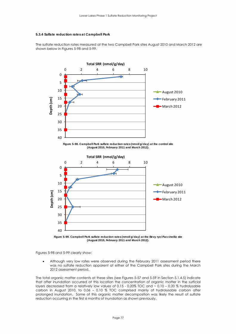
Lower Lakes Phase 1 Sulfate Reduction Monitoring Project
Page 77
5.3.4 Sulfate reduction rates at Campbell Park The sulfate reduction rates measured at the two Campbell Park sites August 2010 and March 2012 are shown below in Figures 5-98 and 5-99.
0
5
10
15
20
25
30
35
40
0 2 4 6 8 10
Depth (cm)
Total SRR (nmol/g/day)
August 2010
February 2011
March 2012
Figure 5-98. Campbell Park sulfate reduction rates (nmol/g/day) at the control site
(August 2010, February 2011 and March 2012).
0
5
10
15
20
25
30
35
40
0 2 4 6 8 10
Depth (cm)
Total SRR (nmol/g/day)
August 2010
February 2011
March 2012
Figure 5-99. Campbell Park sulfate reduction rates (nmol/g/day) at the Bevy rye/Puccinellia site
(August 2010, February 2011 and March 2012). Figures 5-98 and 5-99 clearly show:
Although very low rates were observed during the February 2011 assessment period there was no sulfate reduction apparent at either of the Campbell Park sites during the March 2012 assessment period.
The total organic matter contents at these sites (see Figures 5-57 and 5-59 in Section 5.1.4.5) indicate that after inundation occurred at this location the concentration of organic matter in the surficial layers decreased from a relatively low values of 0.15 - 0.20% TOC and ~ 0.10 – 0.20 % hydrolysable carbon in August 2010, to 0.06 – 0.10 % TOC comprised mainly of hydrolysable carbon after prolonged inundation. Some of this organic matter decomposition was likely the result of sulfate reduction occurring in the first 6 months of inundation as shown previously.

Lower Lakes Phase 1 Sulfate Reduction Monitoring Project
Page 78
It is most probable that the observed substantial decreases in sulfate reduction rates in February 2011 at these sites compared to those observed in August 2010 are due to the near exhaustion of the initially low organic matter content in these sediments, as a result of sulfate reduction since inundation in August 2010. In March 2012 the content of organic matter remained very low and apparently acted as the constraint on sulfate reduction at this study area.

Lower Lakes Phase 1 Sulfate Reduction Monitoring Project
Page 79
5.4 Discussion
5.4.1 Remediation of acidified sediment layers The data from the March 2012 assessment clearly support the findings of Sullivan et al. (2011) showing that both the acidity and low pHs of many of the acidified acid sulfate sediment layers at the study areas are being remediated by a number of processes and sources that deliver organic carbon and alkalinity to these layers. These include: Movement of the alkalinity that is contained in the lake waters - and derived from the River
Murray water - entering the sediment profile via either convective or diffusive processes. The unvegetated control sites at both Tolderol and Campbell Park where the other likely sources of alkalinity addressed in this study are either absent or negligible, are instructive in assessing the magnitude of the contribution of this source of alkalinity in the remediation of acidified acid sulfate sediments. Figures 5-33 and 5-47 both indicate that the diffusion of the substantial alkalinity in the lake waters is capable of causing appreciable increases in sediment pH down to 30 cm depth within a few months. For example, at Tolderol control site the pH of the 0 - 10 cm layer initially 2.4 prior to inundation (May 2010) and 3.0 after inundation (August 2010), rose to a pH of 5.7 by November 2010. Similarly, at Campbell Park control site the pH of the 0 - 10 cm layer initially 3.7 prior to inundation (August 2010), rose to a pH of 4.3 by November 2010 and then to 6.4 by February 2011. The data from this study confirms these trends with continued increases in pH evident at the March 2012 assessment at both of these sites especially in the deeper sediment layers. This data showing the neutralising trends in both of the unvegetated and formerly strongly acidified sites strongly suggests that even left unvegetated, these formerly degraded lake sediments will slowly remediate via the movement of alkalinity into the sediments if surface water is present.
Alkalinity from added solid phase liming materials. Ultra-fine Robe lime was added to the
surface layers at only two of the treatment sites; the Juncus and Phragmites treatments at Waltowa. The pH data from field sampling (Sullivan et al. 2011) clearly showed that this application resulted in elevated pHs in the top 0 – 20 cm sediment layers with pHs between 7 and 8.8 pre-inundation, much higher that the pHs of between 4.7 and 6.7 observed at this time in the unlimed Cotula treatment and Waltowa. However, the effect of such liming materials are often localised and this is exemplified by subsurface sediment layers at both the Juncus and Phragmites treatments at Waltowa having pHs < 5 during the study period.
Alkalinity already existing in the sediments (i.e. the sediment’s Acid Neutralising Capacity (ANC)).
As may be expected from recently severely acidified surface soil layers the ANC contents of the 0 - 40 cm surficial layers were negligible apart from those two treatments discussed above that had received additions of Aglime and the sediments as Poltalloch down to 20 cm depth (where there were only minor sporadic occurrences of CaCO3). Similarly, the Titratable Actual Alkalinity values of these surficial sediment layers were also generally very low. The data in Sullivan et al. (2011) indicated that the ANC of the exposed acidified lake sediments was negligible (unless Aglime had been applied) and unable to supply alkalinity to remediate acidity upon lake refilling.
Alkalinity derived from sulfate reduction. The data in Sullivan et al. (2011) and in this study clearly
show that sulfate reduction has taken place where organic materials have been added to the lake sediments by revegetation. Whether this process results in the net production of alkalinity is anymore than only minor or ephemeral quantities will be discussed in a later section (see Section 5.4.2).
Sullivan et al. (2011) clearly showed that there are two main constraints against sulfate reduction in the formerly exposed lake sediments:
1. Lack of organic matter, and 2. Severely acidified (i.e. pH < 4) sediment layers.
The severe acidification constraint was discussed at length in Sullivan et al. (2011) and only the organic matter constraint will be addressed here. Organic matter Organic matter in the lake sediments (as noted previously in Sullivan et al. 2010a & 2011) is very low. The data in this study demonstrates that the organic matter content of these sediments has been greatly increased by the bioremediation program using the establishment of vegetation. However, different vegetation produces organic matter in different amounts and over different time periods.

Lower Lakes Phase 1 Sulfate Reduction Monitoring Project
Page 80
For example, annual plants like Bevy rye produce appreciable amounts of vegetation relatively quickly but then die, leaving dead dry straw-like residue. In contrast perennial plants like Phragmites and Juncus continue to produce organic matter: it is clear from the Waltowa study area that Phragmites could successfully resist prolonged flooding to greater inundation depths than the Juncus species planted at this location. These different patterns of organic matter production and capacity clearly affected sulfate reduction rates. This is best shown by both the TOC and sulfate reduction data from the Waltowa study area. Waltowa: The organic matter supply differed markedly between the three treatments (Phragmites, Cotula and Juncus) at Waltowa. The Phragmites treatment continued to produce abundant organic matter and thus maintained high TOC levels even during the March 2012 assessment (Figure 5-20), whereas the production of organic matter in both the Cotula and Juncus treatments, ceased after substantial inundation (and certainly by the February 2011 and March 2012 assessments) resulting in TOC depletions in the uppermost sediment layers (Figures 5-22 and 5-24). The comparative sulfate reduction data for this study area (Figure 5-88) indicates that the ability of Phragmites to continue to supply the surficial 0 – 20 cm sediment layer with organic matter even after relatively deep inundation has greatly enhanced the rates of sulfate reduction as compared to the two other vegetation types that had completely submerged, died and undergone decomposition soon after inundation in August 2010.
5.4.2 The nature of sulfur cycling and organic matter decomposition during the initial inundation of the Lower Lakes sediments It is clear that the provision of organic matter in these sediments by revegetation has generally resulted in sulfate reduction to take place. The nature of the sulfate reduction process was dependent on the supply of organic matter that varied according to the type of vegetation used for bioremediation including such factors as whether the vegetation is perennial or annual, and importantly, whether the vegetation can maintain viability and productivity after inundation. However, the data also indicate that the alkalinity supplied to the sediments by sulfate reduction during the assessment period generally occurs via a sulfur cycling process that will be only ephemeral and relatively minor. The data at all locations where sulfate reduction occurred at appreciable rates, indicate a common process of sulfate reduction in these sediments upon bioremediation by revegetation as described in Figure 5-100 below:
Figure 5-100. Conceptual diagram of sulfur cycle operating in the upper layers of the bioremediated inundated Lower Lakes sediments.

Lower Lakes Phase 1 Sulfate Reduction Monitoring Project
Page 81
This conceptual diagram shows that sulfate is reduced during organic matter decomposition (often in microsites around the roots of the plants) used for bioremediation. The sulfide (e.g. H2S) released from this process is mainly converted to elemental sulfur (S8o(s)). This could be by either chemical means (reaction with O2, or manganese and iron oxides) as per the equations below:
O2 + 2H2S → ¼ S80(S) + 2H2O [5.1]
2Fe(OH)3(s) + H2S + 4H+ → 1/8 S80(S) + 2Fe2+ + 6H2O [5.2]
MnO2(s) + H2S + 4H+ → 1/8 S80(S) + Mn2+ + 2H2O [5.3] The data at some of the sites showing intense sulfate reduction during the February 2011 assessment (e.g. Tolderol vegetated site in the uppermost soil layer) did show gradual removal of manganese and iron upon prolonged inundation as well as greatly increased Fe2+ contents in the surfical sediment pore-waters after inundation (Sullivan et al. 2011). These findings are consistent with the process described in Equations 5.2 and 5.3 above operating. The observed decreases in both HCl-extractable manganese and iron such as observed in both Sullivan et al. (2011) and this study and the observed increases in Fe2+ concentrations in the sediment pore-waters may also have occurred as a result of manganese oxides and iron oxides acting as electron acceptors during the decomposition of organic matter. Another possible formation pathway of elemental sulfur in this system is via bacterial oxidation of the sulfide produced by sulfate reduction (e.g. Elsgaard and Jørgensen 1992). It is important that there was formation and accumulation at the March 2012 assessment of appreciable quantities of both iron monosulfides and pyrite in the surficial sediment layers when organic matter is non-limiting to continued sulfate reduction (i.e. under the Phragmites site at Waltowa). Elemental sulfur was the most common product forming during the sulfate reduction rate determinations. However, in the sediments under the Phragmites site at Waltowa the contents of elemental sulfur (Figure 5-19) were minimal compared to the contents of both pyrite and AVS (Figures 5-13 and 5-16, respectively). One typical mechanism for this transformation is as below (e.g. Berner, 1984):
FeS + S80 → FeS2 [5.4]
Other pathways to pyrite formation involve the reaction of monosulfide with the dissolution products of elemental sulfur, especially polysulfides (Rickard, 1997; Rickard and Luther, 1997), such as:
FeS + Sn2- → FeS2 + Sn-12- [5.5] Elemental sulfur can also oxidise back to sulfate soon after formation using O2 or Fe3+ (Burton et al. 2006a) as below:
1/8S8o(s) + 3/2O2 + H2O → SO42- + 2H+ [5.6]
1/8S8o(s) + 6Fe3+ + 4 H2O → SO42- + 6Fe2+ + 8H+ [5.7] Elemental sulfur can also undergo bacterial disproportionation (Thamdrup et al. 1993) as below:
1/2S8o(s) + 4H2O → 3H2S + SO42- + 2H+ [5.8] The sulfate reduction process as a result of bioremediation using vegetation on the exposed sediments of the Lower Lakes will be an acidity-neutral process unless potential acidity is stored in sulfides, or acidity is lost from the system (e.g. elemental sulfur gets entrained in overlying lake waters and oxidises there), or acidity from elemental sulfur oxidation escapes from sediment into lake waters. The data from this study indicate that appreciable alkalinity arising from sulfate reduction in these systems and stored as pyrite and monosulfides is occurring only under the Phragmites site as Waltowa (where organic matter is being produced in the sediments 19 months post-inundation). Such alkalinity production was minimal for all of the other sites be they bioremediated or not, during the initial period (~ 19 months) of inundation. The formation of an MBO layer on the sediments under the Phragmites site at Waltowa and within the top 5 cm of these sediments was observed during the 2012 assessment indicating that appreciable monosulfides as well as pyritic sulfur are accumulating in and over the sediments at this location under Phragmites.

Lower Lakes Phase 1 Sulfate Reduction Monitoring Project
Page 82
Although the avoidance of the accumulation of appreciable quantities of elemental sulfur, monosulfides and disulfides in the surficial lake sediments after bioremediation – apart from under the Phragmites vegetation - results in negligible net production of alkalinity in the upper lake sediments, this may be regarded as a positive outcome as this situation also results in the avoidance of some key possible future hazards that were important foci of this study. These are:
1. there was no appreciable development of potential sulfidic acidity in these surface layers over the duration of the study – apart from under the Phragmites vegetation. Thus during any future drying events if lake levels are lowered sufficiently to expose sediments, the hazard of rapid surface acidification that may have been present if for example pyrite had accumulated in these layers, should not be realised. However, pyrite has begun to accumulate in appreciable quantities after even 19 months of inundation under the Phragmites. This represents a potential acidification hazard due to sulfide accumulation that may continue to develop at longer inundation durations than those able to be observed in this study, especially in areas where lake vegetation such as Phragmites continues to supply organic matter that can fuel further sulfate reduction in such sediments.
2. there was no appreciable development of monosulfides in these surface layers – again apart from under the Phragmites vegetation - over the duration of the study. Thus the hazards of both deoxygenation and metal accumulation (as monosulfides) in the sediment surface layers did not develop to any appreciable extent during the short to medium (i.e. ~ 0.2 to 2 years) period of this study apart from under Phragmites. Such hazards may continue to develop at longer inundation durations than those able to be observed in this study, in areas where lake vegetation such as Phragmites continues to supply organic matter that can fuel further sulfate reduction in these sediments.
5.4.3 Metal and metalloid dynamics in the sediments resulting from bioremediation The mobility of metals is likely to be affected by numerous factors and processes operating in the bioremediated sediments. These include the effects on metal mobility of the increased pH of the sediments (often after the initial decrease in pH due to exchange of acidity) most likely (as discussed previously) arising mainly from movement of alkalinity downward from inundating lake waters. Another process that often affects metal mobility in sediments experiencing appreciable sulfate reduction is the sequestration of metals in the low-solubility sulfides that can accumulate under such conditions. However as discussed previously, the accumulation of both monosulfides and disulfides (e.g. pyrite) in these sediments was – apart from under the Phragmites vegetation - minimal due to the nature of the sulfur cycling (see Figure 5-100). Thus the sequestration within sulfides of appreciable quantities of metals or metalloids was not likely during the initial inundation of these lake sediments apart from under the Phragmites vegetation. In addition, and as shown in Figure 5-100, the processes of sulfur cycling and organic matter decomposition can independently impact on the mobility of metal oxides especially iron oxides and oxyhydroxides and manganese oxides. As these two phases are, of course, comprised of metals and are known for their ability to adsorb a wide range of metals it is likely that the bioremediation may have affected the mobility of a range of metals in these sediments. Indeed, the data from the March 2012 assessment continue to show appreciable systematic changes in Fe mobility following the initial inundation of these lake sediments. Iron concentrations have generally appreciably increased after inundation (e.g. Figure 5-101). Differences in the mobility of Fe and other metals may become more pronounced during longer durations of inundation as the sediments sweep through a wider range of biogeochemical regimes than occurred during the initial inundation of these lake sediments, especially where living bioremediation vegetation that survived the inundation of the lakes continue to provide organic matter to drive these geochemical regime changes. In addition it is likely that the general changes in Eh (towards more reducing) and pH (from acidic to neutral) of the sediments have begun to drive the reductive dissolution of iron minerals such as jarosite as is indicated by the distinctive iron macromorphology exhibited in Figures 3-9 and 3-10. The HCl-extractable Zn concentrations generally increased in the sediments (see Figures 9-105 – 9-112, Appendix 6) presumably as a result of the increased Fe mineral dissolution that has resulted in the increased in Fe concentrations in these sediments. There were no consistent observable changes in HCl-extractable As, Cr, Cu, Ni or Pb during the inundation of these lake sediments to

Lower Lakes Phase 1 Sulfate Reduction Monitoring Project
Page 83
date, however, it should be noted that this study did not replicate the February 2011 study examining pore-water metal concentrations in these sediments.
0
5
10
15
20
25
30
35
40
0 500 1000 1500 2000 2500Depth (cm)
Fe (mg/kg)
May 2010
August 2010
November 2010
February 2011
March 2012
Figure 5-101. Tolderol total iron dynamics at the Juncus in Bevy rye site (May 2010 – March 2012).
5.4.4 Nutrient dynamics in the sediments resulting from bioremediation The production and consumption of nutrients in sediments is very likely to be affected by numerous factors and processes operating in the bioremediated sediments. These include the mineralisation of the nutrients contained in the organic matter provided by the bioremediating vegetation. The decomposition of organic matter in freshwater environments can occur under either aerobic or anaerobic conditions. Under aerobic conditions oxygen is used to facilitate decomposition whereas under anaerobic conditions the lack of oxygen forces bacteria to use other terminal electron acceptors. Nitrates are a nutrient that can be used for this process in place of oxygen and are energetically favoured relative to the use of sulfate for this purpose, but generally if sulfate is present in adequate concentration it fulfils this role leading to sulfate reduction (sulfides are inhibitory to nitrification (Joye and Hollibaugh 1995)). If sulfate is not present in adequate amounts then carbon in organic matter can be used to facilitate decomposition of organic matter (albeit at very slow rates) and methane will be produced (i.e. methanogenesis). In marine water affected sediments the terminal electron acceptor is predominantly sulfur, whereas in freshwater sediments it is carbon (Harris 1999). The presence of sulfate in appreciable concentrations can greatly increase the rate of organic matter decomposition and nutrient mineralisation in sediments (Jørgenson 1982). Caraco et al. (1989) proposed that phosphorus release from freshwater sediments correlates with the sulfate concentration of the overlying water. The work of Lamers and co-workers (e.g. Lamers et al. 2002) confirm this for sulfate-polluted freshwater wetlands. Therefore, it was proposed by Sullivan et al. (2011) that it was likely that continued enhanced sulfate reduction under the living lake vegetations such as Phragmites may also increase the release of phosphates (and other nutrients) from sediments. The nutrient data gained from Sullivan et al. (2011) showed few general trends during inundation through to February 2011, apart from a considerable decrease in ammonium during that period. It was noted in that study that such changes may become more pronounced during later stages of inundation as the sediments sweep through a wider range of biogeochemical regimes than occurred during the initial inundation of these lake sediments especially where living bioremediation vegetation that survived the inundation of the lakes continue to provide organic matter to drive these geochemical regime changes. This study shows that such changes in nutrients have happened at the longer durations of inundation at the Waltowa study area, where large decreases in ammonia concentrations in the pore-waters of the deeper (i.e. 20 – 40 cm) sediment layers has occurred under the Phragmites cf. under the Cotula

Lower Lakes Phase 1 Sulfate Reduction Monitoring Project
Page 84
and Juncus (Figure 5-102) presumably due to uptake by the living Phragmites. No such systematic changes in ammonia occurred under the other study areas.
0
5
10
15
20
25
30
35
40
0 5 10 15 20 25Depth (cm)
Ammonia (mg/L N)
Phragmites
Cotula
Juncus
Phragmites MBO
Figure 5-102. Pore-water ammonia characteristics at the Waltowa study area (March 2012).
Similarly the Phragmites has greatly increased the concentration of orthophosphate in the pore-waters of the surface sediment layers (i.e. 0 – 5 cm) cf. under the Cotula and Juncus in the Waltowa study area (Figure 5-103); presumably due to enhanced mineralisation of phosphate from accumulated organic matter consequent of sulfate reduction. The considerable decrease in TOC in these uppermost sediment layers at this site from the February 2011 assessment to the March 2012 assessment (Figure 5-20) supports this proposition. It is likely that these Phragmites sediments may be a source of phosphate to the overlying lake waters.
0
5
10
15
20
25
30
35
40
0.00 0.50 1.00 1.50
Depth (cm)
Orthophosphate (mg/L P)
Phragmites
Cotula
Juncus
Phragmites MBO
Figure 5-103. Pore-water orthophosphate characteristics at the Waltowa study area (March 2012).

Lower Lakes Phase 1 Sulfate Reduction Monitoring Project
Page 85
6.0 Conclusions The key findings of this study are: 1) Considerable sulfate reduction was occurring during the March 2012 assessment only in the
surface sediment layers where organic matter is continuing to be provided when the vegetation used for bioremediation are species that survived lake re-filling (i.e. Phragmites). There were clear on-going differences in the effectiveness of the bioremediation vegetation in driving this process. Whereas the annual plants and short perennial plants (relative to the inundation depth) produce appreciable amounts of organic matter but then die, tall perennial plants that survive inundation can continue to produce organic matter. This is important because in sediments such as these where the availability of organic matter is the main constraint against sulfate reduction, the patterns of organic matter accumulation and production dictate the consequent patterns of sulfate reduction. Importantly, Phragmites, which successfully resisted prolonged inundation, is clearly continuing to supply organic matter to sediments long after inundation and hence is continuing to strongly drive sulfate reduction processes.
2) The March 2012 assessment clearly shows that appreciable quantities of reduced inorganic
sulfides (especially pyrite and monosulfides) were accumulating in surface sediment layers under the Phragmites treatment. As well as representing an appreciable amount of alkalinity produced in these sediments from sulfate reduction processes, this store of pyrite also represents an appreciable and likely growing potential sulfidic acidity hazard in the surface lake sediments under this bioremediation treatment. Similarly, the store of monosulfidic materials (i.e. Monosulfidic Black Oozes (MBOs)) under the Phragmites treatment also represents the development of associated acidification, metal mobilisation and deoxygenation hazards under this bioremediation treatment.
Given their location in the surface layers of sediments when an inundation tolerant bioremediation species, in this case Phragmites, was used as for bioremediation, this potential sulfidic acidity hazard would be realised much earlier than would previously have been the case, should the Lower Lakes experience atmospheric exposure as was the case in the last drought.
The accumulation of appreciable quantities of pyrite (and hence the development of such a considerable potential sulfidic acidity hazard) was not observed, and given the lack of an organic matter supply, is unlikely to occur when vegetation used for bioremediation is inundation intolerant and undergoes death during inundation.
3) Both the acidity and low pHs of the acidified acid sulfate sediment layers are continuing to be
remediated by a number of processes and sources some consequent of the bioremediation, some not.
The two main factors effecting on-going acidity remediation are: o the movement into the sediment of the alkalinity that is contained in the lake waters and; o the vegetation established during bioremediation when inundation tolerant adding alkalinity
indirectly to the soil via provision of organic matter and thus enabling sulfate reduction resulting in the accumulation of reduced inorganic sulfides (especially pyrite and monosulfides).
4) The data indicate appreciable increases both in ferrous iron (Fe2+) concentrations in pore-waters
and in the HCl-extractable zinc (Zn) concentrations in the sediments during the study period. 5) The data indicate that, apart from under the Phragmites, there were few general trends in
nutrient availability consequent of bioremediation at the March 2012 assessment. However, two strong trends in nutrient mobility were observed under the Phragmites with large decreases in ammonia concentrations in the pore-waters of the deeper (i.e. 20 – 40 cm) sediment layers and greatly increased phosphate concentrations in the pore-waters of the surface sediment likely due to enhanced mineralisation of phosphate from accumulated organic matter consequent of sulfate reduction. It is likely that these sediments under Phragmites may be a source of phosphate to the overlying lake waters.

Lower Lakes Phase 1 Sulfate Reduction Monitoring Project
Page 86
7.0 Recommendations 1) Southern Cross University is aware that this study has focused on the geochemical processes and
changes that have occurred in the relatively early stages of lake re-filling and likely ecological and biogeochemical restoration. This is unlikely to be a major limitation for the examination of sulfate-reduction associated processes for those bioremediated sites where the organic matter produced by the bioremediation vegetation was largely removed or exhausted during this and the February 2011 assessment. However it is an important consideration when assessing the possible long-term effects of bioremediation using vegetation that is still producing organic materials or where there was (at the end of our study) still a relative abundance of organic matter to drive further changes to the biogeochemistry of the lake sediments. It is also an important consideration when assessing the possible long-term effects of de-acidification of the lake sediments on metal and metalloid mobilisation as non-sulfate reduction associated alkalinity drives sediments from being strongly acidic to neutral to alkaline. Differences in geochemical behaviour to those observed in this study may develop during later stages of inundation as the sediments sweep through a wider range of biogeochemical regimes than occurred initially, especially but not only, where living bioremediation vegetation that survived the inundation of the lakes continue to provide organic matter to drive such geochemical regime changes. Such changes could result in the development of the hazards that can be associated with sulfate reduction such as the accumulation of sulfides such as monosulfides and pyrite, hazards that were avoided during the initial 6 month period of lake infilling but have started to develop after another 13 months. It is our recommendation that future monitoring of the effects of bioremediation on the geochemistry of the lake sediments, by assessment programs similar to that used in this project, be undertaken to fully assess both the medium and long term effects of the various bioremediation techniques on the lake ecosystem.
2) The March 2012 results showing appreciable build up of HCl-extractable zinc: when taken in conjunction with the results of the February 2011 assessment also indicate that attention needs to be paid to the mobility of metals in these sediments especially nickel and zinc. In a lake setting, including sites treated by bioremediation techniques, there are a number of important scenarios where subsurface bio-available trace metals could enter the surface aquatic ecosystem. This includes ingestion by burrowing benthic organisms, translocation into plants via roots (this is an especially important consideration for lake sediment bioremediation via revegetation) and direct ingestion by foraging animals (e.g. birds and fish). As such, the fate and possible mobility of subsurface pore-water nickel and zinc at these sites requires consideration from both a geochemical perspective (i.e. developing the knowledge required to predict how pore-water nickel and zinc concentrations will change into the future) and an ecological perspective (i.e. examining nickel and zinc uptake in potentially exposed organisms). It is our recommendation that future monitoring of the pore-water nickel and zinc in the lake sediments as affected by bioremediation is required in order to assess ongoing environmental risks posed by the presence of very high bio-accessible concentrations of these two potentially-toxic trace metals (nickel and zinc).
3) The March 2012 results show a strong trend in nutrient mobility under the Phragmites with large increases in the concentrations of phosphate in the pore-waters of the surface sediments indicating that it is likely that these Phragmites sediments may be a source of phosphate to the overlying lake waters. It is our recommendation that future monitoring of nutrients in the lake sediments as affected by bioremediation is required in order to assess the ongoing environmental risks posed by the presence of an enhanced source of phosphate to the overlying lake waters provided by bioremediation using Phragmites.

Lower Lakes Phase 1 Sulfate Reduction Monitoring Project
Page 87
4) The results also confirms the results of Sullivan et al. (2011) that the different vegetation types
used for bioremediation had very different organic matter production characteristics and that these differences markedly affected the sediment’s geochemical behaviour during the first 19 months of lake re-filling. The results of this study strongly indicate the need for a further detailed study on both: i. the effectiveness of the different vegetation types and strategies used for bioremediation,
and ii. the unbioremediated lake sediment behaviour. Such understanding is required in order to understand in sufficient detail the reasons for these different sediment behaviours and to provide a factual basis to optimise lake bioremediation strategies and to understand the lake’s ecological restoration. It is our recommendation that such a study be undertaken.

Lower Lakes Phase 1 Sulfate Reduction Monitoring Project
Page 88
8.0 References Ahern C.R., L.A. Sullivan and A.E. McElnea. 2004. Laboratory methods guidelines 2004 - acid sulfate
soils. In: 'Queensland Acid Sulfate Soil Technical Manual'. (Department of Natural Resources, Mines and Energy: Indooroopilly, Queensland).
Ahonen L. and O. Tuovinen. 1991. Temperature effects on bacterial leaching of sulfide minerals in
shake flask experiments. Appl. Environ. Microbiol. 57: 138–145. Alpers C.N. and D.K. Nordstrom. 1999. Geochemical modelling of water-rock interactions in mining
environments. p. 289–323. In: Plumee G.S., Logsdon M.J. (Eds.) ‘The environmental geochemistry of mineral deposits.’ Vol 6. Rev. Econ. Geology.
Aneja V.P. 1990. Natural sulfur emissions into the atmosphere. JAPCA J. Air Waste Manag. 40: 469-76. ANZECC/ARMCANZ. 2000. 'Australian and New Zealand guidelines for fresh and marine water
quality.' (Australian and New Zealand Environment and Conservation Council, Agricultural and Resource Management Council of Australia and New Zealand: Canberra). http://hermes.erin.gov.au/pls/crg_public/!CRGPPUBLIC.PSTART?strAction=SearchByChemical
APHA. 2005 'Standard methods for the examination of water and wastewater (21st Ed.).' (American
Public Health Association - American Water Works Association: Baltimore, USA). Åström M. 1998. Partitioning of transition metals in oxidised and reduced zones of sulphide-bearing
fine-grained sediments. App. Geochem. 13: 607-617. Åström M. and N. Corin. 2000. Abundance, source and speciation of trace elements in humus-rich
streams affected by acid sulfate soils. Aquat. Geochem. 6: 367-383. Åström M. 2001. Effect of widespread severely acidic soils on spatial features and abundance of
trace elements in steams. J. Geochem. Explor. 73: 181-191. Bartlett R.W. 1973. A combined pore diffusion and chalcopyrite dissolution kinetics model for in situ
leaching of a fragmented copper porphyry. p. 331–374. In: D.J.I. Evans and R.S. Shoemaker (Ed.) International Symposium on Hydrometallurgy. Chicago, Ill.
Bates T.S., B.K. Lamb, A. Guether, J. Dignon and R.E. Stoiber. 1992. Sulfur emissions to the atmosphere
from natural sources. J. Atmos. Chem. 14: 315-37. Berner R.A. 1984. Sedimentary pyrite formation: an update. Geochim. Cosmochim. Acta 48: 605-615. Berresheim H., P.H.Wine and D.D. Davis. 1995. Sulfur in the atmosphere. p. 251-307. In: Composition,
chemistry, and climate of the atmosphere. Singh, H.B. (Ed.). New York: Van Nostrand Reinhold. Bigham J.M., U. Schwertmann and L. Carlson. 1992. Mineralogy of precipitates formed by the
biogeochemical oxidation of Fe(II) in mine drainage. p. 219-232. In: Biomineralization Processes of Iron and Manganese – Modern and Ancient Environments (Eds. HCW Skinner and RW Fitzpatrick), Catena Supplement 21.
Bigham J.M., U. Schwertmann, S.J. Traina, R.L. Winland and M. Wolf. 1996. Schwertmannite and the
chemical modeling of iron in acid sulfate waters. Geochim. Cosmochim. Acta 60: 2111–2121. Blodau C. 2006. A review of acidity generation and consumption in acidic coal mine lakes and their
watersheds. Sci. Total Env. 369: 307-332. Bloomfield C. and J.K. Coulter. 1973. Genesis and management of acid sulfate soils. Adv. Agron. 25:
265–326. Braun R.L., A.E. Lewis and M.E. Wadsworth. 1974. In-place leaching of primary sulfide ores: Laboratory
leaching data and kinetics model. Metall. Trans. 5: 1717–1726. Burton E.D., R.T. Bush, S.G. Johnston, L.A. Sullivan and A.F. Keene. 2011. Sulfur biogeochemical cycling
and novel Fe-S mineralization pathways in a tidally re-flooded wetland. Geochim. Cosmochim. Acta. 75: 3434-3451.

Lower Lakes Phase 1 Sulfate Reduction Monitoring Project
Page 89
Burton E.D., R.T. Bush and L.A. Sullivan. 2006a. Elemental sulfur in drain sediments associated with acid sulfate soils. Appl. Geochem. 21: 1240–1247.
Burton E.D., R.T. Bush and L.A. Sullivan. 2006b. Reduced inorganic sulfur speciation in drain sediments
from acid-sulfate soil landscapes. Env. Sci. Tech. 40: 888-893. Burton E.D., R.T. Bush and L.A. Sullivan. 2006c. Acid-volatile sulfide oxidation in coastal floodplain
drains: iron-sulfur cycling and effects on water quality. Env. Sci. Tech. 40: 1217-1222. Burton E.D., R.T. Bush and L.A. Sullivan. 2006d. Sedimentary iron geochemistry in acidic waterways
associated with coastal lowland acid sulfate soils. Geochim. Cosmochim. Acta 70: 5455-5468. Burton E.D., R.T. Bush, L.A. Sullivan, R.K. Hocking, D.R.G. Mitchell, S.G. Johnston, R.W. Fitzpatrick, M.
Raven, S. McClure and L.Y. Jang. 2009. Iron-Monosulfide Oxidation in Natural Sediments: Resolving Microbially Mediated S Transformations Using XANES, Electron Microscopy, and Selective Extractions. Env. Sci. Tech. 43: 3128-3134.
Burton E.D., R.T. Bush, L.A. Sullivan, S.G. Johnston and D.R.G. Mitchell. 2008a. Mobility of arsenic and
selected metals during re-flooding of iron- and organic-rich acid-sulfate soil. Chem. Geol. 253: 64-73.
Burton E.D., R.T. Bush, L.A. Sullivan and D.R.G. Mitchell. 2007. Reductive transformation of iron and
sulfur in schwertmannite-rich accumulations associated with acidified coastal lowlands. Geochim. Cosmochim. Acta 71: 4456 - 4473.
Burton E.D., S.G. Johnston, K. Watling, R.T. Bush A.F. Keene and L.A. Sullivan. 2010. Arsenic effects and
behavior in association with the Fe(II)-catalysed transformation of schwertmannite. Env. Sci. Tech. 44: 2016–2021.
Burton E.D., L.A. Sullivan, R.T. Bush, S.G. Johnston and A.F. Keene. 2008b. A simple and inexpensive
chromium-reducible sulfur method for acid-sulfate soils. Appl. Geochem. 23: 2759-2766. Bush R.T., R. McGrath and L.A. Sullivan. 2004a. Occurrence of marcasite in an organic-rich Holocene
mud. Aust. J. Soil Res. 42, 617–622. Bush R.T., D. Fyfe and L.A. Sullivan. 2004b. Occurrence and abundance of monosulfidic black ooze in
coastal acid sulfate soil landscapes. Aust. J. Soil Res. 42: 609-616. Bush R.T. and L.A. Sullivan. 1997. Morphology and behaviour of greigite from a Holocene sediment in
eastern Australia. Aust. J. Soil Res. 35: 853–861. Bush R. T., L.A. Sullivan, D. Fyfe and S.J. Johnston. 2004c. Redistribution of monosulfidic black oozes by
floodwaters in a coastal acid sulfate soil floodplain. Aust. J. Soil Res. 42: 603-607. Bush R.T., L.A. Sullivan and C. Lin. 2000. Iron monosulfide distribution in three coastal floodplain acid
sulfate soils, eastern Australia. Pedosphere 10: 237–246. Callinan R.B., J. Sammut and G.C. Fraser. 2005. Dermatitus, bronchitis and mortality in empire
gudgeon Hypseleotris compressa exposed naturally to run-off from acid sulfate soil. Dis. Aquati. Organ. 63: 247-253.
Canfield D.E., B. Thamdrup and S. Fleischer. 1998. Isotope fractionation and sulfur metabolism by
pure and enrichment cultures of elemental sulfur-disproportionating bacteria. Limnol. Oceanogr. 43: 253–264.
Caraco N.F. 1989. Evidence for sulphate-controlled phosphate release from sediments of aquatic
ecosystems. Nature 341: 316-318. Charlson R.J., J.E. Lovelock, M.O. Andreae and S.G. Warren. 1987. Oceanic phytoplankton,
atmospheric sulfur, cloud albedo and climate. Nature 326: 655-61. Claff S.R., L.A. Sullivan, E.D. Burton and R.T. Bush. 2010. A sequential extraction for acid sulfate soils:
Partitioning of iron. Geoderma 155: 244-230. Cline I.D. 1969. Spectrophotometric determination of hydrogen sulfide in natural waters. Limn.
Oceanog. 14: 454-458.

Lower Lakes Phase 1 Sulfate Reduction Monitoring Project
Page 90
Cornell R.M. and U. Schwertmann. 2003. The Iron Oxides. Wiley-VCH. Weinheim. Corfield J. 2000. The effects of acid sulfate soil run-off on a subtidal estuarine macrobenthic
community in the Richmond River, NSW, Australia. ICES J. Mar. Sci. 57: 1517-1523. Davis G.B. and A.I.M. Ritchie. 1986. A model of oxidation in pyritic mine wastes: Part 1. Equations and
approximate solution. Appl. Math. Model. 10: 314–322. DENR. 2010. Acid sulfate soils research program summary report. Prepared by the Lower Lakes Acid
Sulfate Soils Research Committee for the SA Department of Environment and Natural Resources, Adelaide.
Dent D.L. 1986. Acid sulfate soils: A baseline for research and development. ILRI Publ. 39. International
Institute for Land Reclamation and Improvement, Wageningen, Netherlands. Dent D.L. and L.J. Pons. 1995. Acid sulphate soils: A world view. Geoderma 67: 263–276. Dent D.L. and R.W. Raiswell. 1982. Quantitative models to predict the rate and severity of acid
sulphate development. p. 73–95. In: H. Dost, and N. van Breemen. 1982. Proceedings of the Bangkok Symposium on Acid Sulfate Soils. ILRI Pub. 31. International Institute for Land Reclamation and Improvement, Wageningen, Netherlands.
Diaz R.J. and R. Rosenberg. 1995. Marine benthic hypoxia: a review of its ecological effects and the
behavioural responses of benthic macrofauna. Oceanography and Marine Biology: An Annual Review 33: 245 - 303.
Dold B. and L. Fontbote. 2001. Element cycling and secondary mineralogy in porphyry copper
tailings as a function of climate, primary mineralogy, and mineral processing. J. Geochem. Exploration 74: 3-55.
Dove M.C. and J. Sammut. 2007. Impacts of estuarine acidification on survival and growth of Sydney
rock oysters Saccostreaglomerata (Gould, 1850). J. Shellfish Res. 26: 519–527. Elsgaard L. and B.B. Jørgensen. 1992. Anoxic transformations of radiolabeled hydrogen sulfide in
marine and freshwater sediments. Geochim. Cosmochim. Acta 56: 2425-2435. EPA. 2003. Toxicological Review of Hydrogen Sulfide. http://www.epa.gov/ iris/toxreviews/0061-tr.pdf. Evangelou V.P. and Y.L. Zhang. 1995. A review: Pyrite oxidation mechanism and acid mine drainage
prevention. Crit. Reviews Environ. Sci. Technol. 25: 141-199. Fanning D. S., M.C. Rabenhorst, S.N. Burch, K.R. Islam and S.A. Tangren. 2002. Sulfides and sulfates. In:
Soil Mineralogy with Environmental Applications (Eds. J. B. Dixon, D. G. Schulze and W. L. Daniels). Soil Science Society of America, Madison, WI.
Fältmarsch R.M., M.E. Åström and K-M. Vuori. 2008. Environmental risks of metals mobilized from acid
sulphate soils in Finland: a literature review. Boreal Env. Res. 13: 444-456. Fitzpatrick R., S. Marvanek, P. Shand, R. Merry and M. Thomas. 2008a. Acid sulfate soil maps of the
River Murray below Blanchetown (Lock 1) and Lakes Alexandrina and Albert when water levels were at pre- drought and current drought conditions. CSIRO Land and Water Glen Osmond, SA.
Fitzpatrick R.W., E. Fritsch and P.G. Self. 1996. Interpretation of soil features produced by ancient and
modern processes in degraded landscapes. V. Development of saline sulfidic features in non-tidal seepage areas. Geoderma 69:1–29.
Fitzpatrick R.W., B. Powell and S. Marvanek. 2008b. Atlas of Australian Acid Sulfate Soils. p. 90–97. In:
Fitzpatrick, R.W. and Shand, P. (Eds.) ‘Inland Acid Sulfate Soil Systems Across Australia’ CRC LEME Open File Report No. 249. (Thematic Volume), CRC LEME, Perth, Australia.
Fitzpatrick R.W. and P. Shand. 2008. Inland Acid Sulfate Soils in Australia: Overview and Conceptual
Models. p. 6–74. In: Fitzpatrick, R.W. and Shand, P. (Eds.) ‘Inland Acid Sulfate Soil Systems Across Australia’ CRC LEME Open File Report No. 249. (Thematic Volume), CRC LEME, Perth, Australia.

Lower Lakes Phase 1 Sulfate Reduction Monitoring Project
Page 91
Fitzpatrick R.W., P. Shand, S. Marvanek, R.H. Merry, M. Thomas, M.D. Raven, S.L. Simpson and S.
McClure. 2008c. Acid sulfate soils in subaqueous, waterlogged and drained soil environments in Lake Albert, Lake Alexandrina and River Murray below Blanchetown (Lock 1): properties, distribution, genesis, risks and management. Report prepared for Department of Environment and Heritage SA. CSIRO Land and Water Report Number 46/08. CSIRO Land and Water, Glen Osmond, SA.
Fitzpatrick R.W., P. Shand and R.H. Merry. 2009. Acid Sulfate Soils. p. 65-111. In: Jennings, J.T. (Ed.)
“Natural History of the Riverlands and Murraylands’. Royal Society of South Australia (Inc.) Adelaide, South Australia.
Fossing H. and B.B. Jørgensen. 1989. Measurement of bacterial sulfate reduction in sediments:
Evaluation of a single-step chromium reduction method. Biogeochem. 8: 205-222. Fossing H., S. Thode-Andersen and B.B. Jørgensen. 1992. Sulfur isotope exchange between 35S-
labeled inorganic sulfur compounds in anoxic marine sediments. Mar. Chem. 38: 117-132. Freney J.R. 1961. Some observations on the nature of organic sulfur compounds in soils. Aust. J. Agric.
Res. 12: 424-432. Froelich P.N., G.P. Klinkhammer, M.L. Bender, N.A. Luedtke, G.R. Heath, D. Cullen, P. Dauphin, D.
Hammond, B. Hartman and V. Maynard. 1979. Early oxidation of organic matter in pelagic sediments of the eastern equatorial Atlantic: suboxic diagenesis. Geochim. Cosmochim. Acta 43: 1075 - 1090.
Georgala D. 1980. Paleoenvironmental Studies of Post-glacial Black Clays in Northern Sweden. PhD
Thesis, University of Stockholm, Sweden. Hamilton S.K., S.J. Sippel, D.F. Calheiros and J.M. Melack. 1997. An Anoxic Event and Other
Biogeochemical Effects of the Pantanal Wetland on the Paraguay River. Limn. Oceanog. 42: 257-272.
Harris G.P. 1999. Comparison of the biogeochemistry of lakes and estuaries: Ecosystem processes,
function groups, hysteresis effects and interactions between macro-and microbiology. Mar. Freshwater Res. 50: 791-811.
Hladyz S. and S. Watkins. 2009. Understanding blackwater events and managed flows in the Edward-
Wakool River system. Fact Sheet p. 2. (Murray-Darling Freshwater Research Centre: Wodonga, Vic).
Howarth R.W. 1979. Pyrite: its rapid formation in a salt marsh and its importance in ecosystem
metabolism. Science 203: 49–51. Howarth R.W. and B.B. Jørgensen. 1984. Formation of 35S-labelled elemental sulfur and pyrite in
coastal marine sediments (Limfjorden and Kysing Fjord, Denmark) during short-term 35SO42- reduction measurements. Geochim. Cosmochim. Acta 48: 1807-1818.
Howitt J.A., D.S. Baldwin, G.N. Rees and J.L. Williams. 2007. Modelling blackwater: Predicting water
quality during flooding of lowland river forests. Ecol. Modelling 203: 229-242. Hsieh Y.P, S.W. Chung, Y.J. Tsau and C.T. Sue. 2002. Analysis of sulfides in the presence of ferric
minerals by diffusion methods. Chem. Geol. 182: 195-201. Jaynes D.B., A.S. Rogowski and H.B. Pionke. 1984. Acid drainage from reclaimed coal strip mines. I.
Model description. Water Resour. Res. 20: 233–242. Johnson D.B. 1993. Biogeochemical cycling of iron and sulfur in leaching environments. FEMS
Microbiol. Rev. 11: 63-70. Johnston S.G., P.G. Slavich and P. Hirst. 2004. The acid flux dynamics of two artificial drains in acid
sulfate soil backswamps on the Clarence River floodplain, Australia. Aust. J. Soil Res. 42: 623-637. Johnston S.G., P.G. Slavich and P. Hirst. 2005. Changes in surface water quality after inundation of
acid sulfate soils of different vegetation cover. Aust. J. Soil Res. 43: 1-12.
Lower Lakes Phase 1 Sulfate Reduction Monitoring Project
Page 92
Johnston S.G., P.G. Slavich, L.A. Sullivan, and P. Hirst. 2003. Artificial drainage of floodwaters from sulfidic backswamps: effects on deoxygenation in an Australian estuary. Marine Freshwater Res., 54: 781-795.
Jørgenson B.B. 1982. Mineralisation of organic matter in the sea bed - the role of sulphate reduction.
Nature 296: 643-645. Jørgensen B.B., H. Fossing, C.O. Wirsen and H.W. Jannasch. 1991. Sulfide oxidation in the anoxic Black
Sea chemocline. Deep-Sea Res. 38: 1083 - 1103. Joye S.B. and J.T. Hollibaugh. 1995. Influence of sulfide inhibition of nitrification on nitrogen
regeneration in sediments. Science 270: 623-625. Konsten C.J.M., N. van Breemen, S. Suping, I.B. Aribawa and J.E. Groenenberg. 1994. Effects of
flooding on pH of rice-producing, acid sulfate soils in Indonesia. Soil Sci. Soc. Am. J. 58: 871-883. Lamers L.P.M., S. Falla, E.M. Samborska, I.A.R. van Dulken, G. van Hengstum and J.G.M. Roelofs. 2002.
Factors controlling the extent of eutrophication and toxicity in sulfate-polluted freshwater wetlands. Limn. Oceanogr. 47: 585-593.
Liu M.S., R.M.R. Branion and D.W. Duncan. 1987. Oxygen transfer to Thiobacillus cultures. p. 375–384.
In: P.R. Norris and D.P. Kelly (Ed.) Biohydrometallurgy: Proceedings of the International Symposium, Warwick, UK.
Ljung K., F. Maley, A. Cook and P. Weinstein. 2009. Acid sulfate soils and human health: A Millennium
Ecosystem Assessment. Env. Int. 35: 1234-1242. Lohmann U. and J. Feichter. 2005. Global indirect aerosol effects: a review. Atmos. Chem. Phys. 5:
715-37. Lundgren D.G. and M. Silver. 1980. Ore leaching by bacteria. Ann. Rev. Microbiol. 34: 263–283. Luther III G.W. 1991. Pyrite synthesis via polysulfide compounds. Geochim. Cosmochim. Acta 55:
2839–2849. Luther III G.W., B. Glazer, S. Ma, R. Trouwborst, B.R. Shultz, G. Drushcel and C. Kraiya. 2003. Iron and
sulfur chemistry in a stratified lake: evidence for iron-rich sulfide complexes. Aquatic Geochem. 9: 87 - 110.
Luther III G.W., B. Sundby, B.L. Lewis, P.J. Brendel, and N. Silverberg. 1997. Interactions of manganese
with the nitrogen cycle: alternative pathways to dinitrogen. Geochim. Cosmochim. Acta 61: 4043- 4052.
Macdonald B.C.T., J. Smith, A.K. Keene, M. Tunks, A. Kinsela and I. White I. 2004a. Impacts from runoff
from sulphuric soils on sediment chemistry in an estuary lake. Sci. Total Environ. 329: 115-130. Macdonald B.C.T., O.T. Denmead, I. White, and M.D. Melville. 2004b. Natural sulfur dioxide emissions
from sulfuric soils. Atmos. Env. 38: 1473-1480. McGuire M.M. and R.J. Hamers. 2000. Extraction and quantitative analysis of elemental sulfur
fromsulfide mineral surfaces by high-performance liquid chromatography. Env. Sci. Tech. 34: 4651-4655.
Millero F.J., S. Hubinger, M. Fernandez and S. Garnett. 1987. Oxidation of H2S in seawater as a
function of temperature, pH and ionic strength. Env. Sci. Tech. 21: 439 - 443. Moreno-Mateos D., M.E. Power, F.A. Comin and R. Yockteng. 2012. Structural and functional loss in
restored wetland ecosystems. PLoS Biol. 10: 1-8. Moses C.O., D.K. Nordstrom, J.S. Hermann and A.L. Mills. 1987. Aqueous pyrite oxidations by dissolved
oxygen and by ferric iron. Geochim. Cosmochim. Acta 51: 1561–1571. Nriagu J.O. 1978. Biogeochemistry of Lead in the Environment, Ecological Cycles, Elsevier,
Amsterdam.

Lower Lakes Phase 1 Sulfate Reduction Monitoring Project
Page 93
Pantelis G. and A.I.M. Ritchie. 1991. Macroscopic transport mechanisms as a rate-limiting factor in dump leaching of pyrite ores. Appl. Math. Model. 15: 136–143.
Pantelis G. and A.I.M. Ritchie. 1992. Rate limiting factors in dumps leaching of pyritic ores. Appl. Math.
Model. 16: 553–560. Piene A., A. Tritschler, K. Kusel and S. Peiffer. 2000. Electron flow in an iron-rich acidic sediment-
evidence for an acidity-driven iron cycle. Limnol. Oceanogr. 45: 1077-87. Ponnamperuma F.N. 1972. The chemistry of submerged soils. Advances in Agronomy 24: 29-96. Ponnamperuma F.N., T. Attanandana and G. Beye. 1973 Amelioration of three acid sulphate soils for
lowland rice. In: 'Proceedings of the International Symposium on acid sulphate soils, 13-20 August 1972, Wageningen, The Netherlands'. (Ed. H Dost) pp. 391-405. (International Institute for Land Reclamation and Improvement, Wageningen, The Netherlands).
Pons L.J. 1973. Outline of the genesis, characteristics, classification and improvement of acid
sulphate soils. In: Dost, H. (Ed.) ‘Acid Sulphate Soils. Proceedings of the International Symposium on Acid Sulphate Soils 13-20 August 1972, Wageningen, The Netherlands. I. Introductory Papers and Bibliography.’ pp. 3-27. Publication No.18, International Institute for Land Reclamation and Improvement, Wageningen, The Netherlands.
Pons L.J. and N. van Breemen. 1982. Factors influencing the formation of potential acidity in tidal
swamps. p. 37–51. In: H. Dost and N. van Breemen. 1982. Proceedings of the Bangkok Symposium on Acid Sulfate Soils. ILRI Pub. 31. International Institute for Land Reclamation and Improvement, Wageningen, Netherlands.
Powell B. and M. Martens. 2005. A review of acid sulfate soil impacts, actions and policies that
impact on water quality in the Great Barrier Reef catchments, including a case study on remediation at East Trinity. Marine Poll. Bull. 51: 149–164.
Preda M. and M.E. Cox. 2001. Trace metals in acid sediments and waters, Pimpama catchment,
southeast Queensland, Australia. Environ. Geol. 40: 755-768. Pronk J. and D.B. Johnson. 1992. Oxidation and reduction of iron by acidophilic bacteria.
Geomicrobiol. J. 10: 153-171. Rabalais N.N. 2002. Nitrogen in aquatic ecosystems. Royal Swedish Academy of Sciences. Ambio 31:
102 -112. Rickard D.T. 1975. Kinetics and mechanisms of pyrite formation at low temperatures. Am. J. Sci. 275:
636–652. Rickard D. 1997. Kinetics of pyrite formation by the H2S oxidation of iron (II) monosulfide in aqueous
solutions between 25 and 125oC: the rate equation. Geochim. Cosmochim. Acta 61: 115–134. Rickard D. and G.W. Luther. 1997. Kinetics of pyrite formation by the H2S oxidation of iron (II)
monosulfide in aqueous solutions between 25 and 125oC: the mechanism. Geochim. Cosmochim. Acta 61: 135–147.
Rickard D. and J.W. Morse. 2005. Acid volatile sulfide (AVS). Mar. Chem. 97: 141–197. Ritsema C.J., Van Mensvoort, M.E.F., Dent, D.L., Tan, Y., Van den Bosch, H. and A.L.M. Van Wijk. 2000.
Acid sulfate soils. In: Handbook of Soil Science, Sumner, M.E. (Ed.). pp G121-G154. CRC Press, Boca Raton, USA.
Rosicky M.A., L.A. Sullivan, P.G. Slavich and M. Hughes. 2004a. Soil properties in and around acid
sulfate soil scalds in the coastal floodplains of New South Wales, Australia. Aust. J. Soil Res. 42: 587-594.
Rosicky M.A., L.A. Sullivan, P.G. Slavich and M. Hughes. 2004b. Factors contributing to the acid
scalding process in the coastal floodplains of New South Wales. Aust. J. Soil Res. 42: 587-594. Rosicky M.A., L.A. Sullivan, P.G. Slavich and M. Hughes. 2006. Techniques for the revegetation of acid
sulfate soil scalds in the coastal floodplains of New South Wales, Australia: ridging, mulching, and liming in the absence of stock grazing. Aust. J. Exp. Agr. 46: 1589-1600.
Lower Lakes Phase 1 Sulfate Reduction Monitoring Project
Page 94
Rozan T.F., M. Taillefert, R.E. Trouwborst, B.T. Glazer, B.T., S. Ma, J. Herszage, L.M. Valdes, K.S. Price and
G.W. Luther III. 2002. Iron, sulfur and phosphorus cycling in the sediments of a shallow coastal bay: implications for sediment nutrient release and benthic macroalgal blooms. Limn. Oceanography 47: 1346 - 1354.
Saltzman E.S. and W.J. Cooper. 1989. Biogenic sulfur in the environment. American Chemical Society,
Washington DC. Sammut J., R.B. Callinan and G.C. Fraser. 1993. The impact of acidified water on freshwater and
estuarine fish populations in acid sulphate soil environments. In: 'Proceedings National Conference on Acid Sulphate Soils'. Coolangatta, Qld. 24-25 June 1993. (Ed. RT Bush) pp. 26-40. (CSIRO, NSW Agriculture, Tweed Shire Council).
Sammut J., R.B. Callinan, and G.C. Fraser. 1996a. An overview of the ecological impacts of acid
sulfate soils in Australia. p. 140–143. In: R.J. Smith (Ed.) Proc. 2nd Nat. Conf. Acid Sulfate Soils. R.J. Smith & Associates and ASSMAC, Alstonville, Australia.
Sammut J., I. White, and M.D. Melville. 1996b. Acidification of an estuarine tributary in eastern
Australia due to drainage of acid sulphate soils. Marine Freshwater Res. 47: 669-684. Sarazin G., G. Michard and F. Prevot. 1999. A rapid and accurate spectroscopic method for alkalinity
measurements in sea water samples. Water Res. 33: 290-294. Silveira M.L., N.B. Comerford, K.R. Reddy, W.T. Cooper and H. El-Rifai. 2008. Characterization of soil
organic carbon pools by acid hydrolysis. Geoderma 144: 405–414. Simpson H.J. and M. Pedini. 1985. Brackishwater aquiculture in the tropics: the problem of acid
sulfate soils. Rome, Italy: Food and Agriculture Organisation of the United Nations. Simpson S., R. Fitzpatrick, P. Shand, B. Angel, D. Spadaro, R. Merry and M. Thomas. 2008. The acid,
metal and nutrient mobilisation following rewetting of acid sulfate soils in the Lower Murray. Prepared for the South Australian Environmental Protection Agency. CSIRO Land and Water Bangor, NSW.
Simpson S.L., R.W. Fitzpatrick, P. Shand, B.M. Angel, D.A. Spadaro and L. Mosley. 2010. Climate-driven
mobilisation of acid and metals from acid sulfate soils. Marine Freshwater Res. 61: 129-138. Stumm W. and J.J. Morgan. 1996. Aquatic chemistry. 3rd Ed., John Wiley & Sons, New York. Sullivan L., E. Burton, R. Bush, K. Watling and M. Bush. 2008. Acid, metal and nutrient mobilisation
dynamics in response to suspension of MBOs in freshwater and to freshwater inundation of dried MBO and sulfuric soil materials. Final Report. A report for "The acid, metal and nutrient mobilisation following rewetting of acid sulfate soils in the Lower Murray Project”. Prepared for the South Australian Environmental Protection Agency. Centre for Acid Sulfate Soil Research, Southern Cross GeoScience, Southern Cross University, Lismore, NSW.
Sullivan L.A., E.D. Burton, N.J. Ward, R.T. Bush, J. Coughran, M.D. Cheetham, D.M. Fyfe, P.J.
Cheeseman and T. McIntyre. 2011. Lower Lakes sulfate reduction study. Prepared for South Australian Department of Environment and Natural Resources. Southern Cross GeoScience Technical Report No. 711, Southern Cross University, Lismore, NSW. 312 pp.
Sullivan L.A. and R.T. Bush. 2000. The behaviour of drain sludge in acid sulfate soil areas: some
implications for acidification of waterways and drain maintenance. In: 'Proceedings of Workshop on Remediation and Assessment of Broadacre Acid Sulfate Soils'. (Ed. P Slavich) pp. 43-48. (Acid Sulfate Soil Management Advisory Committee (ASSMAC): Southern Cross University, Lismore).
Sullivan L.A. and R.T. Bush. 2004. Iron precipitate accumulations associated with waterways in
drained coastal acid sulfate landscapes of eastern Australia. Marine Freshwater Res. 55: 727-736. Sullivan L.A., R.T. Bush, and D. Fyfe. 2002. Acid sulfate soil drain ooze: distribution, behaviour and
implications for acidification and deoxygenation of waterways. p. 91-99. In: Acid sulfate soils in Australia and China. (Eds. C. Lin, M. Melville and L.A. Sullivan), Science Press, Beijing, China .
Lower Lakes Phase 1 Sulfate Reduction Monitoring Project
Page 95
Sullivan L.A., R.T. Bush, N.J. Ward, D.M. Fyfe, M. Johnston, E.D. Burton, P. Cheeseman, M. Bush, C.
Maher, M. Cheetham, K.M. Watling, V.N.L Wong, R. Maher and E. Weber. 2010a. Lower Lakes laboratory study of contaminant mobilisation under seawater and freshwater inundation. Prepared by Southern Cross GeoScience for the SA Department of Environment and Natural Resources, Adelaide.
Sullivan L.A., J.F. Parr, N.J. Ward, R.T. Bush, D.M. Fyfe, M. Bush and R. Hagan. 2012. Lower Lakes
carbon project. Prepared by Southern Cross GeoScience for the SA Department of Environment and Natural Resources, Adelaide.
Sullivan L.A., K.M. Watling, A. McElnea, C. Ahern, E.D. Burton, S. Johnston, A. Keene and R.T. Bush.
2010b. Improved assessment of Acid Neutralising Capacity in acid sulfate soil. In: Co-operative Research Centre for Contamination Assessment and Remediation of the Environment Annual Conference, Adelaide 21-22 July 2010.
Tan Y. 1996. Comments on modeling of oxygen transport and pyrite oxidation in acid sulfate soils by
Bronswijk et al., J. Environ. Qual. 25: 928–930. Thamdrup B., K. Finster, J.W. Hansen and F. Bak. 1993. Bacterial disproportionation of elemental sulfur
coupled to chemical reduction of iron or manganese. Appl. Environ. Microbiol. 59: 101-108. Tuong T.P. 1993. An overview of water management on acid sulfate soils. p. 265–281. In: D.L. Dent
and M.E.F. van Mensvoort (Ed.) Selected Papers of the Ho Chi Minh City Symposium on Acid Sulfate Soils. ILRI Pub. 53. International Institute for Land Reclamation and Improvement, Wageningen, Netherlands.
van Breemen N. 1973. Soil forming processes in acid sulphate soils. In: 'Proceedings of the
International Symposium on acid sulphate soils. 13-20 August 1972, Wageningen, The Netherlands'. (Ed. H Dost), Wageningen, The Netherlands. pp. 66- 129. (International Institute for Land Reclamation and Improvement).
van Breemen N. 1976. Genesis and solution chemistry of acid sulphate soils in Thailand. Agric. Res.
Rep. 848. PUDOC, Wageningen, Netherlands. White I., M.D. Melville, B.P. Wilson and J. Sammut. 1997. Reducing acidic discharges from coastal
wetlands in eastern Australia. Wetland Ecol. 5: 55-72. Wilson B.P., I. White and M.D. Melville. 1999. Floodplain hydrology, acid discharge and changing
water quality associated with a drained acid sulfate soil. Marine Freshwater Res. 50: 149-157. Wong V.N.L., S.G. Johnston, R.T. Bush, L.A. Sullivan, C. Clay, E.D. Burton and P.G. Slavich. 2010. Spatial
and temporal changes in estuarine water quality during a post-flood hypoxic event. Estuarine, Coastal and Shelf Sci. 87: 73–82.

Lower Lakes Phase 1 Sulfate Reduction Monitoring Project
Page 96
9.0 Appendices

Lower Lakes Phase 1 Sulfate Reduction Monitoring Project
Page 97
APPENDIX 1. Site and sample descriptions
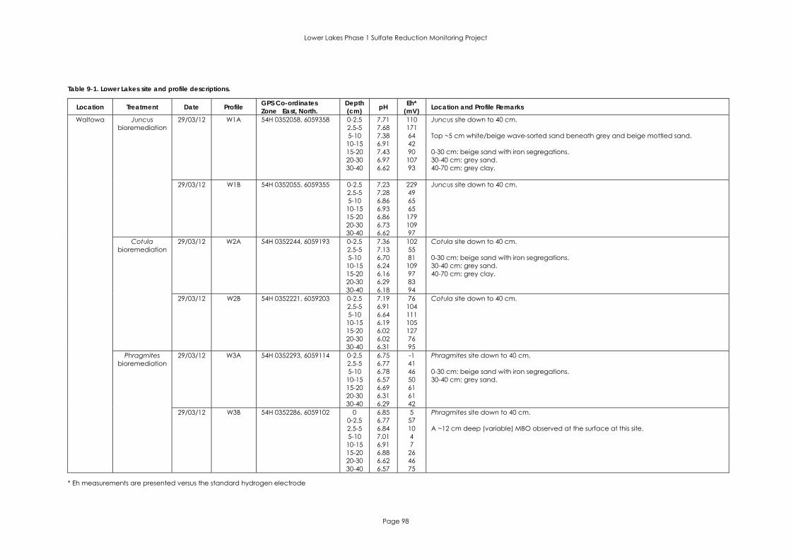
Lower Lakes Phase 1 Sulfate Reduction Monitoring Project
Page 98
Table 9-1. Lower Lakes site and profile descriptions.
Location Treatment Date Profile GPS Co-ordinates Zone East, North.
Depth (cm) pH Eh*
(mV) Location and Profile Remarks
Waltowa Juncus bioremediation
29/03/12 W1A 54H 0352058, 6059358
0-2.5 2.5-5 5-10 10-15 15-20 20-30 30-40
7.71 7.68 7.38 6.91 7.43 6.97 6.62
110 171 64 42 90 107 93
Juncus site down to 40 cm. Top ~5 cm white/beige wave-sorted sand beneath grey and beige mottled sand. 0-30 cm: beige sand with iron segregations. 30-40 cm: grey sand. 40-70 cm: grey clay.
29/03/12 W1B 54H 0352055, 6059355
0-2.5 2.5-5 5-10 10-15 15-20 20-30 30-40
7.23 7.28 6.86 6.93 6.86 6.73 6.62
229 49 65 65 179 109 97
Juncus site down to 40 cm.
Cotula bioremediation
29/03/12 W2A 54H 0352244, 6059193
0-2.5 2.5-5 5-10 10-15 15-20 20-30 30-40
7.36 7.13 6.70 6.24 6.16 6.29 6.18
102 55 81 109 97 83 94
Cotula site down to 40 cm. 0-30 cm: beige sand with iron segregations. 30-40 cm: grey sand. 40-70 cm: grey clay.
29/03/12 W2B 54H 0352221, 6059203
0-2.5 2.5-5 5-10 10-15 15-20 20-30 30-40
7.19 6.91 6.64 6.19 6.02 6.02 6.31
76 104 111 105 127 76 95
Cotula site down to 40 cm.
Phragmites bioremediation
29/03/12 W3A 54H 0352293, 6059114
0-2.5 2.5-5 5-10 10-15 15-20 20-30 30-40
6.75 6.77 6.78 6.57 6.69 6.31 6.29
-1 41 46 50 61 61 42
Phragmites site down to 40 cm. 0-30 cm: beige sand with iron segregations. 30-40 cm: grey sand.
29/03/12 W3B 54H 0352286, 6059102
0 0-2.5 2.5-5 5-10 10-15 15-20 20-30 30-40
6.85 6.77 6.84 7.01 6.91 6.88 6.62 6.57
5 57 10 4 7
26 46 75
Phragmites site down to 40 cm. A ~12 cm deep (variable) MBO observed at the surface at this site.
* Eh measurements are presented versus the standard hydrogen electrode

Lower Lakes Phase 1 Sulfate Reduction Monitoring Project
Page 99
Table 9-1 (continued). Lower Lakes site and profile descriptions.
Location Treatment Date Profile GPS Co-ordinates Zone East, North.
Depth (cm) pH Eh*
(mV) Location and Profile Remarks
Poltalloch 2009 plantings of Bevy Rye
bioremediation
30/03/12 P1A 54H 0341295, 6070677 0-2.5 2.5-5 5-10 10-15 15-20 20-30 30-40
6.48 6.81 6.95 6.87 6.79 4.61 4.32
299 162 131 231 210 359 372
Bevy Rye site down to 40 cm. 0-3 cm: wave washed beige sand. 3-11 cm: dark grey sand. 11-32 cm: light grey sand with frequent orange segregations. >32 cm: grey sand.
30/03/12 P1B 54H 0341267, 6070659 0-2.5 2.5-5 5-10 10-15 15-20 20-30 30-40
7.04 6.96 7.18 7.11 6.99 6.98 6.87
188 194 173 217 224 255 317
Bevy Rye site down to 40 cm. 0-3 cm: wave washed beige sand. 3-11 cm: dark grey sand. 11-32 cm: light grey sand with frequent orange segregations. >32 cm: grey sand.
Campbell Park
Scald (no bioremediation)
30/03/12 CP1A 54H 0340786, 6056740
0-2.5 2.5-5 5-10 10-15 15-20 20-30 30-40
6.81 6.60 5.99 4.32 3.45 3.11 3.21
109 89 114 196 256 313 344
Scald (no bioremediation) site down to 40 cm. Jarosite still around 15-30 cm layer. 0-2 cm: wave washed sand. 2-10 cm: grey sand. 10-30 cm: light grey sand with jarosite. 30-60 cm: blue grey clay.
30/03/12 CP1B 54H 0340772, 6056761
0-2.5 2.5-5 5-10 10-15 15-20 20-30 30-40
6.48 6.83 5.88 4.84 3.20 3.00 3.06
142 100 126 248 350 362 345
Scald (no bioremediation) site down to 40 cm.
2010 seeded with Bevy rye
and Puccinellia bioremediation
30/03/12 CP2A 54H 0340734, 6056750
0-2.5 2.5-5 5-10 10-15 15-20 20-30 30-40
6.67 6.31 6.02 4.88 3.54 3.40 3.37
323 139 141 275 400 420 328
Bevy rye and Puccinellia bioremediation site down to 40 cm.
30/03/12 CP2B 54H 0340728, 6056756
0-2.5 2.5-5 5-10 10-15 15-20 20-30 30-40
7.14 6.91 6.40 6.05 4.99 3.56 3.47
228 158 122 154 292 394 405
Bevy rye and Puccinellia bioremediation site down to 40 cm.
* Eh measurements are presented versus the standard hydrogen electrode

Lower Lakes Phase 1 Sulfate Reduction Monitoring Project
Page 100
Table 9-1 (continued). Lower Lakes site and profile descriptions.
Location Treatment Date Profile GPS Co-ordinates Zone East, North.
Depth (cm) pH Eh*
(mV) Location and Profile Remarks
Tolderol 2010 planted Juncus into
2009 plantings of Bevy Rye
bioremediation
31/03/12 T1A 54H 0331148, 6083496
0-2.5 2.5-5 5-10 10-15 15-20 20-30 30-40
7.17 7.50 7.48 6.71 6.27 6.51 5.92
388 389 254 163 311 243 245
Juncus into plantings of Bevy Rye bioremediation site down to 40 cm. 0-30 cm: beige sand with lots of iron segregations at 20-50 cm, iron band at 30 cm. 30-45 cm: beige sand with jarosite band at 40-45 cm. 45-60 cm: grey sand with some iron segregations. 60-80 cm: grey sand.
31/03/12 T1B 54H 0331160, 6083485
0-2.5 2.5-5 5-10 10-15 15-20 20-30 30-40
7.15 7.04 7.22 6.62 5.97 6.43 5.54
201 172 191 274 249 370 344
Juncus into plantings of Bevy Rye bioremediation site down to 40 cm.
Scald (no bioremediation)
31/03/12 T2A 54H 0331075, 6083416
0-2.5 2.5-5 5-10 10-15 15-20 20-30 30-40
6.07 6.34 6.28 5.94 5.64 4.45 3.58
355 149 154 160 213 304 433
Scald (no bioremediation) site down to 40 cm. Iron-rich crust on some scald surface layers. Jarosite still around 25 cm and lower layers. 0-40 cm: beige sand with very occasional jarosite in roots. 40-50 cm: beige sand with abundant jarosite in roots. 50-60 cm: dark grey sandy clay with abundant jarosite in roots. 60-80 cm: dark grey sandy clay but no jarosite.
31/03/12 T2B 54H 0331047, 6083414
0-2.5 2.5-5 5-10 10-15 15-20 20-30 30-40
7.74 7.27 7.18 6.64 6.74 6.55 6.29
351 161 289 236 286 292 288
Scald (no bioremediation) site down to 40 cm. Iron-rich crust on some scald surface layers. Jarosite still around 25 cm and lower layers.
* Eh measurements are presented versus the standard hydrogen electrode

Lower Lakes Phase 1 Sulfate Reduction Monitoring Project
Page 101

Lower Lakes Phase 1 Sulfate Reduction Monitoring Project
Page 102
APPENDIX 2. Characteristics of soil materials

Lower Lakes Phase 1 Sulfate Reduction Monitoring Project
Page 103
Table 9-2. Characteristics of the Waltowa soil materials, March 2012.
Profile ID* (Site
Code, Core)
Depth Range (cm)
Moisture Content
(%)
pH 1:5 soil:
water
EC 1:5
soil:water (µS/cm)
pHKCl TAA (mol H+ t-1)
ANC (%
CaCO3)
TAAlk (mol
OH- t-1)
Retained acidity
(mol H+ t-1)
Pyritic Sulfur (%S)
Elemental Sulfur (%S)
Acid Volatile Sulfide (%SAV)
Net acidity (mol H+
t-1)
Total C
(%C)
Total N
(%N)
Hydrolysable C
(%C)
Total Organic
C (%C)
W 1A 0-2.5 19.42 9.10 350 9.26 0.00 0.11 11.44 0.00 <0.01 0.001 <0.01 -14.64 0.14 0.003 0.08 0.13 W 1A 2.5-5 17.75 9.48 129 9.23 0.00 0.21 8.70 0.00 <0.01 0.001 <0.01 -27.72 0.13 0.005 0.06 0.13 W 1A 5-10 19.71 9.37 416 9.56 0.00 0.19 16.74 0.00 <0.01 0.003 <0.01 -24.86 0.19 0.006 0.06 0.17 W 1A 10-15 19.82 9.24 962 9.43 0.00 0.34 17.14 0.00 <0.01 0.003 <0.01 -45.34 0.24 0.012 0.05 0.19 W 1A 15-20 19.52 9.14 693 9.35 0.00 0.29 13.87 0.00 <0.01 0.001 <0.01 -38.75 0.22 0.014 0.04 0.18 W 1A 20-30 19.21 8.77 829 7.78 0.00 0.07 3.94 0.00 <0.01 0.002 <0.01 -9.64 0.18 0.010 0.01 0.18 W 1A 30-40 20.02 7.27 1243 6.43 1.08 0.00 0.00 0.00 0.08 0.001 <0.01 53.21 0.20 0.012 0.04 0.21 W 1B 0-2.5 19.14 9.31 282 9.43 0.00 0.22 12.43 0.00 <0.01 0.003 0.02 -19.37 0.17 0.006 <0.01 0.14 W 1B 2.5-5 20.65 9.33 351 9.68 0.00 0.32 26.64 0.00 <0.01 0.007 0.02 -31.14 0.26 0.013 0.15 0.26 W 1B 5-10 19.67 8.98 378 7.90 0.00 0.18 3.74 0.00 <0.01 0.003 <0.01 -23.41 0.14 0.006 <0.01 0.13 W 1B 10-15 19.81 9.19 470 8.52 0.00 0.11 6.22 0.00 <0.01 0.002 <0.01 -14.94 0.14 0.008 0.02 0.12 W 1B 15-20 19.01 9.03 622 8.57 0.00 0.10 5.92 0.00 <0.01 0.003 <0.01 -13.83 0.13 0.007 0.02 0.13 W 1B 20-30 20.32 8.53 897 7.60 0.00 0.06 4.22 0.00 <0.01 <0.001 <0.01 -7.55 0.21 0.014 0.02 0.21 W 1B 30-40 19.33 7.82 1004 6.85 0.00 0.03 2.87 0.00 0.02 <0.001 <0.01 10.33 0.26 0.022 0.05 0.24 W 2A 0-2.5 19.50 9.24 379 8.88 0.00 0.20 6.97 0.00 <0.01 0.002 <0.01 -26.56 0.16 0.011 0.07 0.14 W 2A 2.5-5 20.89 8.44 346 6.97 0.00 0.08 3.77 0.00 <0.01 0.004 <0.01 -10.37 0.23 0.014 0.06 0.22 W 2A 5-10 19.95 7.67 403 6.72 0.00 0.22 4.28 0.00 <0.01 0.005 <0.01 -29.92 0.25 0.026 0.02 0.14 W 2A 10-15 20.68 7.18 534 6.43 2.51 0.00 0.00 0.00 <0.01 0.002 <0.01 2.51 0.22 0.019 0.03 0.20 W 2A 15-20 22.90 6.47 705 5.97 3.25 0.00 0.00 0.00 0.03 <0.001 <0.01 20.27 0.32 0.029 0.04 0.32 W 2A 20-30 27.14 6.51 894 5.92 3.57 0.00 0.00 0.00 0.06 <0.001 <0.01 42.87 0.40 0.042 0.04 0.34 W 2A 30-40 48.59 6.46 2560 6.43 2.82 0.00 0.00 0.00 0.40 <0.001 <0.01 252.15 2.09 0.226 0.38 2.08 W 2B 0-2.5 19.37 9.33 303 8.82 0.00 0.12 8.70 0.00 <0.01 0.001 <0.01 -16.37 0.16 0.012 <0.01 0.16 W 2B 2.5-5 18.62 8.57 276 7.26 0.00 0.09 3.34 0.00 <0.01 0.003 <0.01 -12.20 0.19 0.018 0.07 0.18 W 2B 5-10 19.74 7.91 356 6.49 0.79 0.00 0.00 0.00 <0.01 0.005 <0.01 0.79 0.19 0.018 0.08 0.18 W 2B 10-15 19.97 7.25 440 5.98 3.03 0.00 0.00 0.00 <0.01 <0.001 <0.01 3.03 0.22 0.016 0.09 0.22 W 2B 15-20 20.49 6.72 575 5.58 3.41 0.00 0.00 0.00 <0.01 <0.001 <0.01 3.41 0.21 0.018 0.10 0.19 W 2B 20-30 21.22 6.54 819 5.79 2.86 0.00 0.00 0.00 <0.01 <0.001 <0.01 2.86 0.23 0.023 0.07 0.23 W 2B 30-40 37.12 7.45 2380 7.17 0.00 0.16 9.87 0.00 0.28 <0.001 <0.01 150.88 0.88 0.096 <0.01 0.88
* See Table 9-1 in Appendix 1 for further details on the treatment.

Lower Lakes Phase 1 Sulfate Reduction Monitoring Project
Page 104
Table 9-2 (continued). Characteristics of the Waltowa soil materials, March 2010.
Profile ID* (Site
Code, Core)
Depth Range (cm)
Moisture Content
(%)
pH 1:5
soil:water
EC 1:5
soil:water (µS/cm)
pHKCl TAA (mol H+ t-1)
ANC (%
CaCO3)
TAAlk (mol
OH- t-1)
Retained acidity
(mol H+ t-1)
Pyritic Sulfur (%S)
Elemental Sulfur (%S)
Acid Volatile Sulfide (%SAV)
Net acidity (mol H+
t-1)
Total C
(%C)
Total N
(%N)
Hydrolysable C
(%C)
Total Organic
C (%C)
W 3A 0-2.5 48.90 9.13 1436 9.29 0.00 9.05 29.41 0.00 0.12 0.010 0.04 -1108.7 2.35 0.122 0.23 1.35 W 3A 2.5-5 23.73 9.50 705 9.71 0.00 1.31 94.02 0.00 0.02 0.004 0.02 -149.92 0.35 0.020 0.08 0.23 W 3A 5-10 20.50 9.08 752 9.00 0.00 0.13 8.69 0.00 <0.01 0.007 <0.01 -17.63 0.21 0.023 0.05 0.18 W 3A 10-15 19.92 8.17 820 7.54 0.00 0.11 4.10 0.00 <0.01 <0.001 <0.01 -14.09 0.15 0.014 0.02 0.15 W 3A 15-20 19.95 7.37 986 6.80 0.00 0.06 3.87 0.00 <0.01 <0.001 <0.01 -7.91 0.16 0.021 0.01 0.16 W 3A 20-30 23.89 6.85 1319 6.10 2.82 0.00 0.00 0.00 <0.01 <0.001 <0.01 2.82 0.29 0.026 0.06 0.29 W 3A 30-40 25.50 6.60 1781 6.11 3.53 0.00 0.00 0.00 0.03 <0.001 <0.01 21.34 0.41 0.039 0.04 0.41 W 3B MBO 90.82 8.04 8490 8.32 0.00 3.43 75.46 0.00 0.30 0.012 0.15 -179.77 6.46 0.626 1.73 6.00 W 3B 0-2.5 50.35 8.87 1524 9.20 0.00 2.06 111.60 0.00 0.05 0.005 0.03 -225.29 1.36 0.100 0.25 1.15 W 3B 2.5-5 24.00 9.22 714 9.69 0.00 0.65 43.28 0.00 0.01 0.004 0.03 -61.37 0.28 0.019 0.05 0.19 W 3B 5-10 20.97 9.12 725 8.88 0.00 0.18 6.21 0.00 <0.01 0.004 <0.01 -24.22 0.16 0.011 0.04 0.12 W 3B 10-15 19.54 8.96 765 8.31 0.00 0.07 4.36 0.00 <0.01 0.002 <0.01 -9.50 0.18 0.018 0.01 0.11 W 3B 15-20 20.55 8.62 880 8.12 0.00 0.09 5.19 0.00 <0.01 0.001 <0.01 -12.36 0.18 0.014 <0.01 0.17 W 3B 20-30 23.59 7.73 1266 7.22 0.00 0.04 3.81 0.00 0.03 <0.001 <0.01 12.74 0.30 0.032 0.09 0.30 W 3B 30-40 27.06 7.33 1583 6.92 0.00 0.11 3.86 0.00 0.18 <0.001 <0.01 97.20 0.42 0.044 0.01 0.42
* See Table 9-1 in Appendix 1 for further details on the treatment.
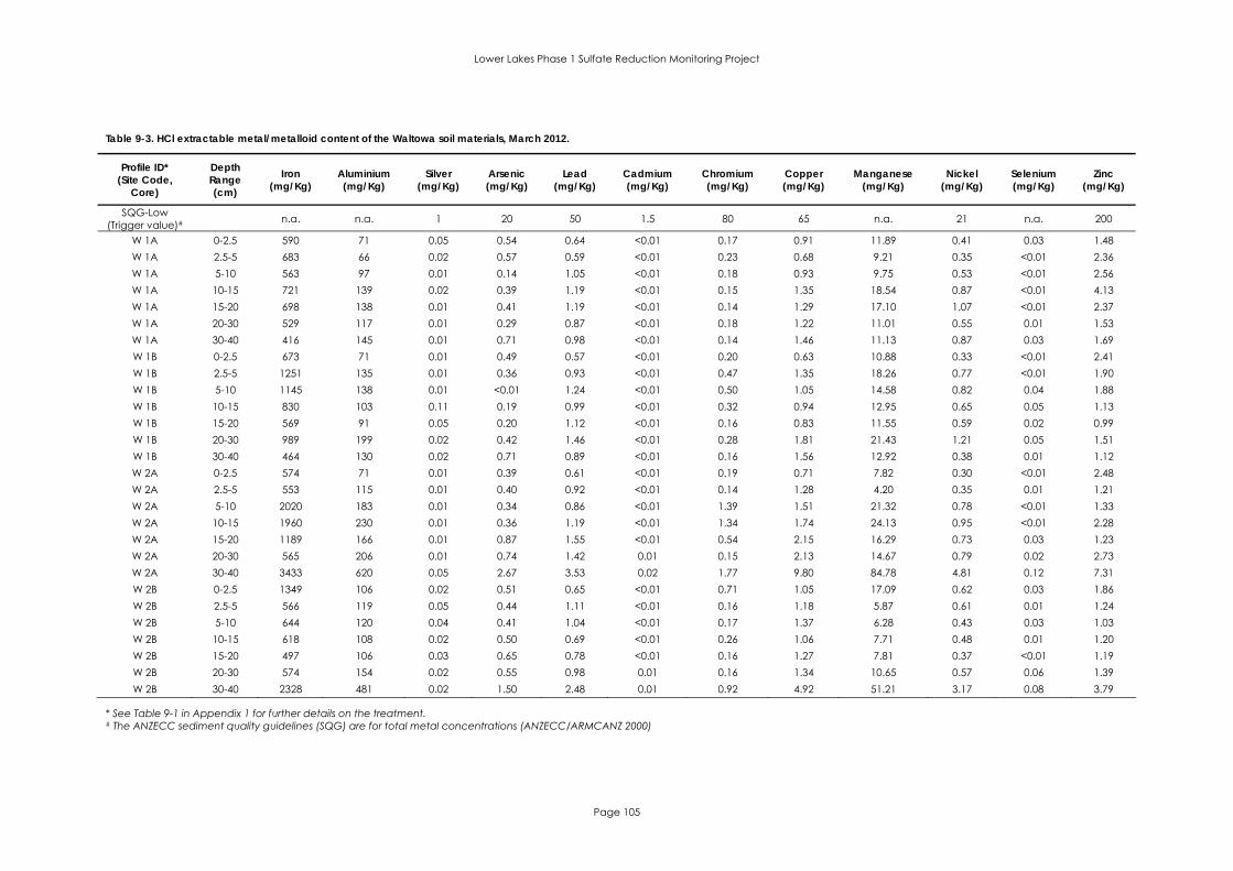
Lower Lakes Phase 1 Sulfate Reduction Monitoring Project
Page 105
Table 9-3. HCl extractable metal/metalloid content of the Waltowa soil materials, March 2012.
Profile ID* (Site Code,
Core)
Depth Range (cm)
Iron (mg/Kg)
Aluminium (mg/Kg)
Silver (mg/Kg)
Arsenic (mg/Kg)
Lead (mg/Kg)
Cadmium (mg/Kg)
Chromium (mg/Kg)
Copper (mg/Kg)
Manganese (mg/Kg)
Nickel (mg/Kg)
Selenium (mg/Kg)
Zinc (mg/Kg)
SQG-Low (Trigger value)# n.a. n.a. 1 20 50 1.5 80 65 n.a. 21 n.a. 200
W 1A 0-2.5 590 71 0.05 0.54 0.64 <0.01 0.17 0.91 11.89 0.41 0.03 1.48 W 1A 2.5-5 683 66 0.02 0.57 0.59 <0.01 0.23 0.68 9.21 0.35 <0.01 2.36 W 1A 5-10 563 97 0.01 0.14 1.05 <0.01 0.18 0.93 9.75 0.53 <0.01 2.56 W 1A 10-15 721 139 0.02 0.39 1.19 <0.01 0.15 1.35 18.54 0.87 <0.01 4.13 W 1A 15-20 698 138 0.01 0.41 1.19 <0.01 0.14 1.29 17.10 1.07 <0.01 2.37 W 1A 20-30 529 117 0.01 0.29 0.87 <0.01 0.18 1.22 11.01 0.55 0.01 1.53 W 1A 30-40 416 145 0.01 0.71 0.98 <0.01 0.14 1.46 11.13 0.87 0.03 1.69 W 1B 0-2.5 673 71 0.01 0.49 0.57 <0.01 0.20 0.63 10.88 0.33 <0.01 2.41 W 1B 2.5-5 1251 135 0.01 0.36 0.93 <0.01 0.47 1.35 18.26 0.77 <0.01 1.90 W 1B 5-10 1145 138 0.01 <0.01 1.24 <0.01 0.50 1.05 14.58 0.82 0.04 1.88 W 1B 10-15 830 103 0.11 0.19 0.99 <0.01 0.32 0.94 12.95 0.65 0.05 1.13 W 1B 15-20 569 91 0.05 0.20 1.12 <0.01 0.16 0.83 11.55 0.59 0.02 0.99 W 1B 20-30 989 199 0.02 0.42 1.46 <0.01 0.28 1.81 21.43 1.21 0.05 1.51 W 1B 30-40 464 130 0.02 0.71 0.89 <0.01 0.16 1.56 12.92 0.38 0.01 1.12 W 2A 0-2.5 574 71 0.01 0.39 0.61 <0.01 0.19 0.71 7.82 0.30 <0.01 2.48 W 2A 2.5-5 553 115 0.01 0.40 0.92 <0.01 0.14 1.28 4.20 0.35 0.01 1.21 W 2A 5-10 2020 183 0.01 0.34 0.86 <0.01 1.39 1.51 21.32 0.78 <0.01 1.33 W 2A 10-15 1960 230 0.01 0.36 1.19 <0.01 1.34 1.74 24.13 0.95 <0.01 2.28 W 2A 15-20 1189 166 0.01 0.87 1.55 <0.01 0.54 2.15 16.29 0.73 0.03 1.23 W 2A 20-30 565 206 0.01 0.74 1.42 0.01 0.15 2.13 14.67 0.79 0.02 2.73 W 2A 30-40 3433 620 0.05 2.67 3.53 0.02 1.77 9.80 84.78 4.81 0.12 7.31 W 2B 0-2.5 1349 106 0.02 0.51 0.65 <0.01 0.71 1.05 17.09 0.62 0.03 1.86 W 2B 2.5-5 566 119 0.05 0.44 1.11 <0.01 0.16 1.18 5.87 0.61 0.01 1.24 W 2B 5-10 644 120 0.04 0.41 1.04 <0.01 0.17 1.37 6.28 0.43 0.03 1.03 W 2B 10-15 618 108 0.02 0.50 0.69 <0.01 0.26 1.06 7.71 0.48 0.01 1.20 W 2B 15-20 497 106 0.03 0.65 0.78 <0.01 0.16 1.27 7.81 0.37 <0.01 1.19 W 2B 20-30 574 154 0.02 0.55 0.98 0.01 0.16 1.34 10.65 0.57 0.06 1.39 W 2B 30-40 2328 481 0.02 1.50 2.48 0.01 0.92 4.92 51.21 3.17 0.08 3.79
* See Table 9-1 in Appendix 1 for further details on the treatment. # The ANZECC sediment quality guidelines (SQG) are for total metal concentrations (ANZECC/ARMCANZ 2000)

Lower Lakes Phase 1 Sulfate Reduction Monitoring Project
Page 106
Table 9-3 (continued). HCl extractable metal/metalloid content of the Waltowa soil materials, March 2010.
Profile ID* (Site Code,
Core)
Depth Range (cm)
Iron (mg/Kg)
Aluminium (mg/Kg)
Silver (mg/Kg)
Arsenic (mg/Kg)
Lead (mg/Kg)
Cadmium (mg/Kg)
Chromium (mg/Kg)
Copper (mg/Kg)
Manganese (mg/Kg)
Nickel (mg/Kg)
Selenium (mg/Kg)
Zinc (mg/Kg)
SQG-Low (Trigger value)# n.a. n.a. 1 20 50 1.5 80 65 n.a. 21 n.a. 200
W 3A 0-2.5 2577 495 0.01 1.37 2.82 0.02 1.12 4.35 96.87 2.77 0.12 5.17 W 3A 2.5-5 1633 161 0.01 0.41 1.61 <0.01 0.81 1.41 25.38 0.90 0.09 1.57 W 3A 5-10 711 116 0.15 0.20 1.33 <0.01 0.26 1.25 8.43 0.52 0.06 1.16 W 3A 10-15 2235 207 0.02 0.47 1.33 <0.01 1.67 1.72 26.02 1.62 0.02 1.33 W 3A 15-20 1883 193 0.01 0.44 1.14 <0.01 1.18 1.86 23.68 1.32 0.01 2.99 W 3A 20-30 816 150 0.03 0.83 1.40 <0.01 0.31 1.69 13.99 0.80 0.03 1.21 W 3A 30-40 1442 324 0.02 0.68 1.70 0.01 0.57 2.87 26.57 1.41 0.05 2.21 W 3B MBO 4434 2007 0.04 4.58 9.28 0.05 0.55 17.71 225.24 7.85 0.48 19.63 W 3B 0-2.5 3294 484 0.02 1.19 2.58 0.01 1.78 4.36 75.44 2.60 0.09 3.85 W 3B 2.5-5 1251 149 0.01 0.37 1.24 <0.01 0.47 1.25 22.58 0.71 <0.01 2.92 W 3B 5-10 658 109 0.02 0.26 1.24 <0.01 0.19 0.97 8.07 0.40 0.06 1.50 W 3B 10-15 646 116 0.03 0.34 1.55 <0.01 0.14 1.00 10.22 0.53 0.05 1.55 W 3B 15-20 1293 205 0.01 0.65 1.62 <0.01 0.41 1.68 18.26 0.99 0.04 1.46 W 3B 20-30 676 165 0.16 1.11 1.40 <0.01 0.16 2.15 13.93 0.81 0.08 1.60 W 3B 30-40 1496 374 0.02 1.33 1.99 0.01 0.67 3.07 34.66 1.45 0.19 2.47
* See Table 9-1 in Appendix 1 for further details on the treatment. # The ANZECC sediment quality guidelines (SQG) are for total metal concentrations (ANZECC/ARMCANZ 2000)
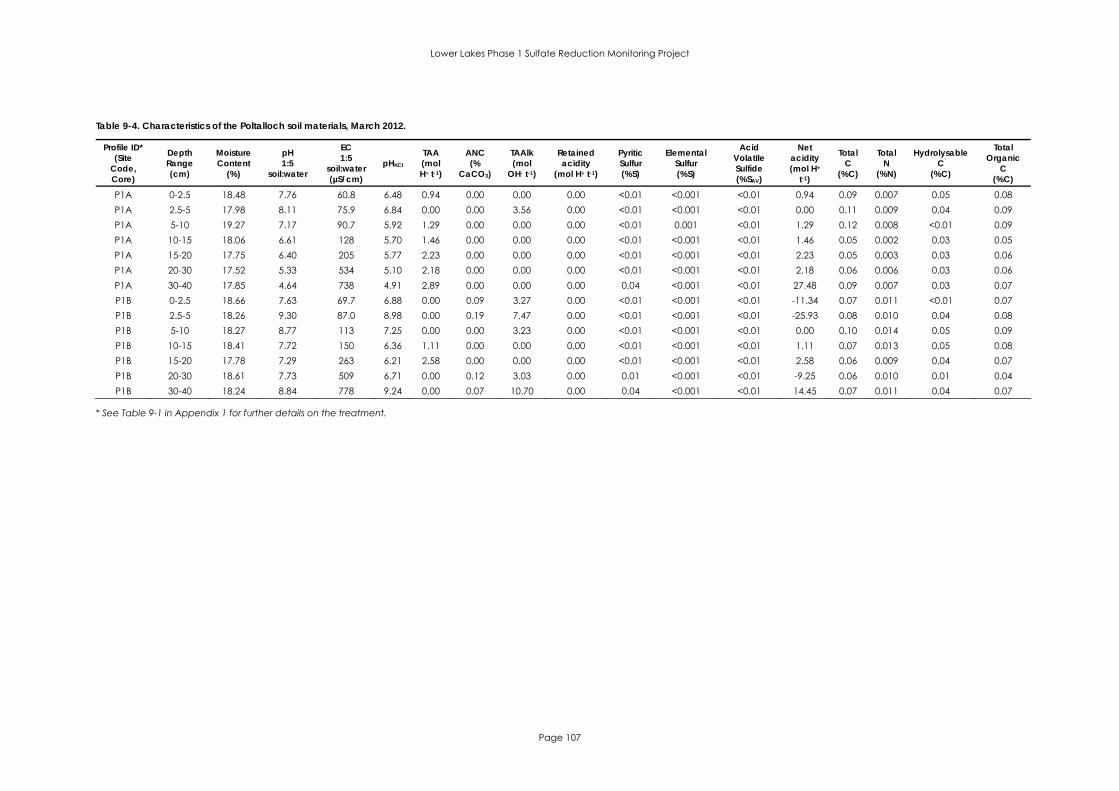
Lower Lakes Phase 1 Sulfate Reduction Monitoring Project
Page 107
Table 9-4. Characteristics of the Poltalloch soil materials, March 2012.
Profile ID* (Site
Code, Core)
Depth Range (cm)
Moisture Content
(%)
pH 1:5
soil:water
EC 1:5
soil:water (µS/cm)
pHKCl TAA (mol H+ t-1)
ANC (%
CaCO3)
TAAlk (mol
OH- t-1)
Retained acidity
(mol H+ t-1)
Pyritic Sulfur (%S)
Elemental Sulfur (%S)
Acid Volatile Sulfide (%SAV)
Net acidity (mol H+
t-1)
Total C
(%C)
Total N
(%N)
Hydrolysable C
(%C)
Total Organic
C (%C)
P1A 0-2.5 18.48 7.76 60.8 6.48 0.94 0.00 0.00 0.00 <0.01 <0.001 <0.01 0.94 0.09 0.007 0.05 0.08 P1A 2.5-5 17.98 8.11 75.9 6.84 0.00 0.00 3.56 0.00 <0.01 <0.001 <0.01 0.00 0.11 0.009 0.04 0.09 P1A 5-10 19.27 7.17 90.7 5.92 1.29 0.00 0.00 0.00 <0.01 0.001 <0.01 1.29 0.12 0.008 <0.01 0.09 P1A 10-15 18.06 6.61 128 5.70 1.46 0.00 0.00 0.00 <0.01 <0.001 <0.01 1.46 0.05 0.002 0.03 0.05 P1A 15-20 17.75 6.40 205 5.77 2.23 0.00 0.00 0.00 <0.01 <0.001 <0.01 2.23 0.05 0.003 0.03 0.06 P1A 20-30 17.52 5.33 534 5.10 2.18 0.00 0.00 0.00 <0.01 <0.001 <0.01 2.18 0.06 0.006 0.03 0.06 P1A 30-40 17.85 4.64 738 4.91 2.89 0.00 0.00 0.00 0.04 <0.001 <0.01 27.48 0.09 0.007 0.03 0.07 P1B 0-2.5 18.66 7.63 69.7 6.88 0.00 0.09 3.27 0.00 <0.01 <0.001 <0.01 -11.34 0.07 0.011 <0.01 0.07 P1B 2.5-5 18.26 9.30 87.0 8.98 0.00 0.19 7.47 0.00 <0.01 <0.001 <0.01 -25.93 0.08 0.010 0.04 0.08 P1B 5-10 18.27 8.77 113 7.25 0.00 0.00 3.23 0.00 <0.01 <0.001 <0.01 0.00 0.10 0.014 0.05 0.09 P1B 10-15 18.41 7.72 150 6.36 1.11 0.00 0.00 0.00 <0.01 <0.001 <0.01 1.11 0.07 0.013 0.05 0.08 P1B 15-20 17.78 7.29 263 6.21 2.58 0.00 0.00 0.00 <0.01 <0.001 <0.01 2.58 0.06 0.009 0.04 0.07 P1B 20-30 18.61 7.73 509 6.71 0.00 0.12 3.03 0.00 0.01 <0.001 <0.01 -9.25 0.06 0.010 0.01 0.04 P1B 30-40 18.24 8.84 778 9.24 0.00 0.07 10.70 0.00 0.04 <0.001 <0.01 14.45 0.07 0.011 0.04 0.07
* See Table 9-1 in Appendix 1 for further details on the treatment.
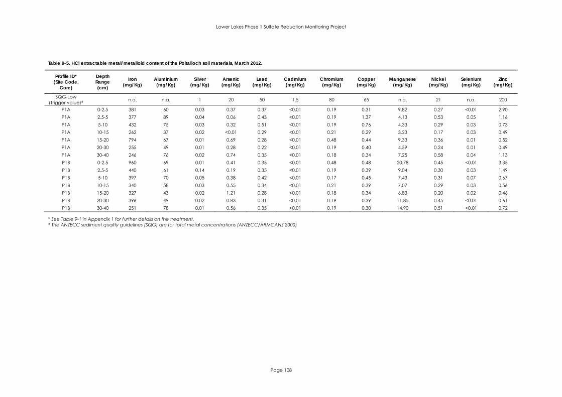
Lower Lakes Phase 1 Sulfate Reduction Monitoring Project
Page 108
Table 9-5. HCl extractable metal/metalloid content of the Poltalloch soil materials, March 2012.
Profile ID* (Site Code,
Core)
Depth Range (cm)
Iron (mg/Kg)
Aluminium (mg/Kg)
Silver (mg/Kg)
Arsenic (mg/Kg)
Lead (mg/Kg)
Cadmium (mg/Kg)
Chromium (mg/Kg)
Copper (mg/Kg)
Manganese (mg/Kg)
Nickel (mg/Kg)
Selenium (mg/Kg)
Zinc (mg/Kg)
SQG-Low (Trigger value)# n.a. n.a. 1 20 50 1.5 80 65 n.a. 21 n.a. 200
P1A 0-2.5 381 60 0.03 0.37 0.37 <0.01 0.19 0.31 9.82 0.27 <0.01 2.90 P1A 2.5-5 377 89 0.04 0.06 0.43 <0.01 0.19 1.37 4.13 0.53 0.05 1.16 P1A 5-10 432 75 0.03 0.32 0.51 <0.01 0.19 0.76 4.33 0.29 0.03 0.73 P1A 10-15 262 37 0.02 <0.01 0.29 <0.01 0.21 0.29 3.23 0.17 0.03 0.49 P1A 15-20 794 67 0.01 0.69 0.28 <0.01 0.48 0.44 9.33 0.36 0.01 0.52 P1A 20-30 255 49 0.01 0.28 0.22 <0.01 0.19 0.40 4.59 0.24 0.01 0.49 P1A 30-40 246 76 0.02 0.74 0.35 <0.01 0.18 0.34 7.25 0.58 0.04 1.13 P1B 0-2.5 960 69 0.01 0.41 0.35 <0.01 0.48 0.48 20.78 0.45 <0.01 3.35 P1B 2.5-5 440 61 0.14 0.19 0.35 <0.01 0.19 0.39 9.04 0.30 0.03 1.49 P1B 5-10 397 70 0.05 0.38 0.42 <0.01 0.17 0.45 7.43 0.31 0.07 0.67 P1B 10-15 340 58 0.03 0.55 0.34 <0.01 0.21 0.39 7.07 0.29 0.03 0.56 P1B 15-20 327 43 0.02 1.21 0.28 <0.01 0.18 0.34 6.83 0.20 0.02 0.46 P1B 20-30 396 49 0.02 0.83 0.31 <0.01 0.19 0.39 11.85 0.45 <0.01 0.61 P1B 30-40 251 78 0.01 0.56 0.35 <0.01 0.19 0.30 14.90 0.51 <0.01 0.72
* See Table 9-1 in Appendix 1 for further details on the treatment. # The ANZECC sediment quality guidelines (SQG) are for total metal concentrations (ANZECC/ARMCANZ 2000)

Lower Lakes Phase 1 Sulfate Reduction Monitoring Project
Page 109
Table 9-6. Characteristics of the Tolderol soil materials, March 2012.
Profile ID* (Site
Code, Core)
Depth Range (cm)
Moisture Content
(%)
pH 1:5
soil:water
EC 1:5
soil:water (µS/cm)
pHKCl TAA (mol H+ t-1)
ANC (%
CaCO3)
TAAlk (mol
OH- t-1)
Retained acidity
(mol H+ t-1)
Pyritic Sulfur (%S)
Elemental Sulfur (%S)
Acid Volatile Sulfide (%SAV)
Net acidity (mol H+
t-1)
Total C
(%C)
Total N
(%N)
Hydrolysable C
(%C)
Total Organic
C (%C)
T 1A 0-2.5 21.41 8.33 55.5 6.63 0.00 0.12 2.42 0.00 <0.01 <0.001 <0.01 -15.62 0.10 0.016 0.08 0.11 T 1A 2.5-5 18.92 7.51 47.9 6.17 3.01 0.00 0.00 0.00 <0.01 <0.001 <0.01 3.01 0.10 0.015 0.07 0.09 T 1A 5-10 18.99 7.04 49.4 6.07 1.79 0.00 0.00 0.00 <0.01 <0.001 <0.01 1.79 0.09 0.013 0.05 0.08 T 1A 10-15 20.39 7.32 102 6.08 3.25 0.00 0.00 0.00 <0.01 <0.001 <0.01 3.25 0.10 0.011 0.03 0.08 T 1A 15-20 20.72 7.06 189 6.11 2.29 0.00 0.00 0.00 <0.01 <0.001 <0.01 2.29 0.09 0.010 0.02 0.07 T 1A 20-30 20.81 7.15 194 6.20 1.09 0.00 0.00 0.00 <0.01 <0.001 <0.01 1.09 0.07 0.012 <0.01 0.05 T 1A 30-40 21.01 5.41 454 5.13 2.18 0.00 0.00 0.00 0.01 <0.001 <0.01 11.41 0.08 0.010 <0.01 0.06 T 1B 0-2.5 21.01 7.72 76.4 6.67 0.00 0.11 2.88 0.00 <0.01 <0.001 <0.01 -14.94 0.10 0.012 0.04 0.08 T 1B 2.5-5 19.67 7.30 73.4 6.27 2.66 0.00 0.00 0.00 0.01 <0.001 <0.01 9.16 0.10 0.013 0.05 0.09 T 1B 5-10 19.90 6.91 100 6.07 3.07 0.00 0.00 0.00 <0.01 <0.001 <0.01 3.07 0.10 0.015 0.07 0.10 T 1B 10-15 19.86 6.56 164 5.81 2.78 0.00 0.00 0.00 <0.01 <0.001 <0.01 2.78 0.14 0.017 0.08 0.14 T 1B 15-20 20.00 7.04 61.9 6.05 2.86 0.00 0.00 0.00 <0.01 <0.001 <0.01 2.86 0.07 0.007 <0.01 0.07 T 1B 20-30 20.37 6.54 133 6.05 1.61 0.00 0.00 0.00 <0.01 <0.001 <0.01 1.61 0.07 0.009 <0.01 0.05 T 1B 30-40 22.26 6.35 353 6.07 1.70 0.00 0.00 0.00 0.14 <0.001 <0.01 87.25 0.10 0.012 <0.01 0.09 T 2A 0-2.5 18.98 6.89 46.7 6.24 2.35 0.00 0.00 0.00 <0.01 <0.001 <0.01 2.35 0.12 0.015 0.01 0.12 T 2A 2.5-5 22.73 6.68 84.9 6.03 3.16 0.00 0.00 0.00 <0.01 <0.001 <0.01 3.16 0.14 0.023 <0.01 0.12 T 2A 5-10 19.42 6.05 35.1 5.46 3.17 0.00 0.00 0.00 <0.01 <0.001 <0.01 3.17 0.08 0.010 0.01 0.08 T 2A 10-15 19.25 6.07 50.8 5.62 3.17 0.00 0.00 0.00 <0.01 <0.001 <0.01 3.17 0.10 0.014 <0.01 0.10 T 2A 15-20 19.29 5.68 35.5 4.97 3.40 0.00 0.00 0.00 <0.01 <0.001 <0.01 3.40 0.09 0.014 0.04 0.09 T 2A 20-30 19.93 4.83 122 4.61 4.78 0.00 0.00 0.00 <0.01 <0.001 <0.01 4.78 0.09 0.009 0.01 0.07 T 2A 30-40 20.92 4.36 255 4.51 7.28 0.00 0.00 0.00 <0.01 <0.001 <0.01 7.28 0.08 0.010 0.01 0.08 T 2B 0-2.5 20.79 7.62 56.5 6.61 0.00 0.11 1.56 0.00 <0.01 <0.001 <0.01 -15.02 0.12 0.013 0.04 0.11 T 2B 2.5-5 21.27 6.82 54.5 6.00 2.60 0.00 0.00 0.00 <0.01 <0.001 <0.01 2.60 0.14 0.013 <0.01 0.12 T 2B 5-10 20.19 6.51 39.1 5.67 2.84 0.00 0.00 0.00 <0.01 <0.001 <0.01 2.84 0.09 0.010 0.01 0.07 T 2B 10-15 20.20 6.24 43.2 5.90 2.78 0.00 0.00 0.00 <0.01 <0.001 <0.01 2.78 0.08 0.009 <0.01 0.07 T 2B 15-20 19.11 5.90 29.3 5.21 2.88 0.00 0.00 0.00 <0.01 <0.001 <0.01 2.88 0.06 0.010 <0.01 0.03 T 2B 20-30 20.40 6.15 38.1 5.66 3.41 0.00 0.00 0.00 <0.01 <0.001 <0.01 3.41 0.09 0.011 <0.01 0.02 T 2B 30-40 20.61 5.83 33.3 5.06 2.93 0.00 0.00 0.00 <0.01 <0.001 <0.01 2.93 0.06 0.009 <0.01 0.04
* See Table 9-1 in Appendix 1 for further details on the treatment.

Lower Lakes Phase 1 Sulfate Reduction Monitoring Project
Page 110
Table 9-7. HCl extractable metal/metalloid content of the Tolderol soil materials, March 2012.
Profile ID* (Site Code,
Core)
Depth Range (cm)
Iron (mg/Kg)
Aluminium (mg/Kg)
Silver (mg/Kg)
Arsenic (mg/Kg)
Lead (mg/Kg)
Cadmium (mg/Kg)
Chromium (mg/Kg)
Copper (mg/Kg)
Manganese (mg/Kg)
Nickel (mg/Kg)
Selenium (mg/Kg)
Zinc (mg/Kg)
SQG-Low (Trigger value)# n.a. n.a. 1 20 50 1.5 80 65 n.a. 21 n.a. 200
T 1A 0-2.5 330 82 0.01 0.09 0.47 <0.01 0.21 0.47 7.20 0.48 <0.01 5.62
T 1A 2.5-5 268 85 0.01 <0.01 0.50 <0.01 0.19 0.54 3.90 0.47 <0.01 1.24
T 1A 5-10 262 71 0.01 <0.01 0.36 <0.01 0.21 0.45 4.60 0.33 <0.01 0.69
T 1A 10-15 181 108 0.01 <0.01 0.35 <0.01 0.18 0.52 5.13 0.36 <0.01 1.58
T 1A 15-20 361 92 0.13 <0.01 0.27 <0.01 0.25 0.42 5.91 0.24 0.03 0.81
T 1A 20-30 1268 142 0.01 <0.01 0.32 <0.01 0.91 0.79 15.78 0.57 0.03 1.20
T 1A 30-40 460 81 0.02 0.30 0.29 <0.01 0.24 0.58 6.56 0.39 <0.01 1.01
T 1B 0-2.5 1274 102 0.01 0.16 0.54 <0.01 0.90 0.72 20.87 0.60 <0.01 4.64
T 1B 2.5-5 1022 119 0.01 0.05 0.52 <0.01 0.70 0.75 14.35 0.54 0.05 1.36
T 1B 5-10 393 82 0.01 0.05 0.45 <0.01 0.26 0.53 5.97 0.46 0.03 0.93
T 1B 10-15 315 108 0.01 0.11 0.60 <0.01 0.17 0.85 6.28 0.39 <0.01 1.07
T 1B 15-20 426 83 0.01 0.09 0.29 <0.01 0.26 0.59 6.19 0.25 0.04 0.86
T 1B 20-30 875 115 0.01 0.14 0.28 <0.01 0.57 0.64 11.27 0.39 <0.01 1.10
T 1B 30-40 2044 199 0.01 0.16 0.45 <0.01 1.62 1.29 24.55 1.03 0.01 3.69
T 2A 0-2.5 1377 109 0.12 0.50 0.54 <0.01 0.49 0.68 12.28 0.50 0.02 1.55
T 2A 2.5-5 1616 182 0.02 0.23 2.60 <0.01 1.15 1.17 19.10 1.00 <0.01 4.27
T 2A 5-10 458 88 0.03 0.44 0.51 <0.01 0.22 0.59 5.21 0.27 <0.01 1.35
T 2A 10-15 1688 214 0.01 0.49 0.68 <0.01 0.97 0.97 20.29 0.65 0.02 1.39
T 2A 15-20 479 100 0.02 0.21 0.47 <0.01 0.20 0.60 5.56 0.19 0.02 0.69
T 2A 20-30 572 105 0.03 0.37 0.57 <0.01 0.20 0.61 6.20 0.24 0.02 0.90
T 2A 30-40 578 116 0.03 0.44 0.35 <0.01 0.19 0.71 7.77 0.24 0.03 0.80
T 2B 0-2.5 1217 105 0.01 0.29 0.59 <0.01 0.56 0.71 14.76 0.48 <0.01 5.94
T 2B 2.5-5 801 146 0.01 0.46 0.65 <0.01 0.43 0.91 8.50 0.37 <0.01 1.48
T 2B 5-10 449 84 0.01 0.17 0.52 <0.01 0.22 0.47 4.49 0.25 0.03 0.79
T 2B 10-15 14632 1251 0.03 3.07 5.27 0.01 9.15 6.12 166.64 6.12 0.18 6.84
T 2B 15-20 4274 664 0.02 2.48 2.81 <0.01 1.96 3.84 53.73 1.84 0.11 3.42
T 2B 20-30 9867 1045 0.02 2.41 2.41 <0.01 6.20 4.95 122.27 3.99 0.13 3.28
T 2B 30-40 5182 666 0.02 1.72 3.36 <0.01 1.74 2.26 43.36 1.50 0.06 3.76
* See Table 9-1 in Appendix 1 for further details on the treatment. # The ANZECC sediment quality guidelines (SQG) are for total metal concentrations (ANZECC/ARMCANZ 2000)

Lower Lakes Phase 1 Sulfate Reduction Monitoring Project
Page 111
Table 9-8. Characteristics of the Campbell Park soil materials, March 2012.
Profile ID* (Site
Code, Core)
Depth Range (cm)
Moisture Content
(%)
pH 1:5 soil:
water
EC 1:5
soil:water (µS/cm)
pHKCl TAA
(mol H+ t-1)
ANC (%
CaCO3)
TAAlk (mol
OH- t-1)
Retained acidity
(mol H+ t-1)
Pyritic Sulfur (%S)
Elemental Sulfur (%S)
Acid Volatile Sulfide (%SAV)
Net acidity (mol H+
t-1)
Total C
(%C)
Total N
(%N)
Hydrolysable C
(%C)
Total Organic
C (%C)
CP 1A 0-2.5 22.77 8.96 421 9.26 0.00 0.24 18.23 0.00 <0.01 <0.001 <0.01 -32.41 0.22 0.027 0.04 0.16 CP 1A 2.5-5 18.90 7.85 332 6.47 1.99 0.00 0.00 0.00 <0.01 <0.001 <0.01 1.99 0.15 0.020 0.05 0.13 CP 1A 5-10 24.86 4.84 597 4.51 6.37 0.00 0.00 0.00 <0.01 <0.001 <0.01 6.37 0.40 0.035 0.14 0.36 CP 1A 10-15 24.15 4.72 574 4.54 12.63 0.00 0.00 0.00 <0.01 <0.001 <0.01 12.63 0.34 0.029 0.02 0.29 CP 1A 15-20 27.96 4.26 878 4.19 19.08 0.00 0.00 17.00 <0.01 <0.001 <0.01 36.08 0.42 0.043 0.07 0.41 CP 1A 20-30 23.38 4.10 782 4.20 12.50 0.00 0.00 3.00 0.07 <0.001 <0.01 57.72 0.28 0.025 0.06 0.26 CP 1A 30-40 38.54 4.30 1642 4.31 25.94 0.00 0.00 14.00 0.46 <0.001 <0.01 323.77 0.55 0.055 0.01 0.50 CP 1B 0-2.5 19.17 9.15 331 9.15 0.00 0.08 10.43 0.00 <0.01 <0.001 <0.01 -10.84 0.13 0.010 0.02 0.08 CP 1B 2.5-5 23.27 9.15 355 8.70 0.00 0.02 7.10 0.00 <0.01 <0.001 <0.01 -2.81 0.09 0.006 0.02 0.06 CP 1B 5-10 20.13 5.26 383 4.94 3.41 0.00 0.00 0.00 <0.01 <0.001 <0.01 3.41 0.20 0.018 0.01 0.17 CP 1B 10-15 22.57 4.24 557 4.22 9.09 0.00 0.00 22.00 <0.01 <0.001 <0.01 31.09 0.27 0.026 0.09 0.26 CP 1B 15-20 23.41 4.17 698 4.24 12.99 0.00 0.00 33.00 <0.01 <0.001 <0.01 45.99 0.30 0.029 0.07 0.28 CP 1B 20-30 31.25 4.14 1138 4.15 25.45 0.00 0.00 5.00 0.12 <0.001 <0.01 105.20 0.43 0.037 0.01 0.40 CP 1B 30-40 52.35 4.11 2650 4.07 47.66 0.00 0.00 23.00 0.87 <0.001 <0.01 614.41 1.07 0.107 0.01 1.04 CP 2A 0-2.5 18.34 9.05 301 8.94 0.00 0.15 8.88 0.00 <0.01 <0.001 <0.01 -19.33 0.10 0.008 0.03 0.06 CP 2A 2.5-5 18.87 7.62 291 6.26 2.94 0.00 0.00 0.00 <0.01 <0.001 <0.01 2.94 0.15 0.010 0.05 0.14 CP 2A 5-10 19.42 5.57 439 5.21 3.18 0.00 0.00 0.00 <0.01 <0.001 <0.01 3.18 0.19 0.011 <0.01 0.16 CP 2A 10-15 21.06 4.43 510 4.38 8.33 0.00 0.00 23.00 <0.01 <0.001 <0.01 31.33 0.20 0.015 0.07 0.19 CP 2A 15-20 22.71 4.53 691 4.49 8.92 0.00 0.00 16.00 <0.01 <0.001 <0.01 24.92 0.21 0.020 <0.01 0.20 CP 2A 20-30 23.48 4.05 894 4.22 11.30 0.00 0.00 6.00 0.04 <0.001 <0.01 39.98 0.26 0.022 0.05 0.22 CP 2A 30-40 34.95 4.05 1741 4.22 24.97 0.00 0.00 12.00 0.45 <0.001 <0.01 315.53 0.46 0.039 0.05 0.44 CP 2B 0-2.5 16.72 8.37 291 7.69 0.00 0.04 3.80 0.00 <0.01 <0.001 <0.01 -5.81 0.11 0.007 0.01 0.06 CP 2B 2.5-5 17.95 7.67 310 6.48 1.10 0.00 0.00 0.00 <0.01 0.004 <0.01 1.10 0.12 0.007 0.05 0.09 CP 2B 5-10 20.48 6.79 424 5.98 2.09 0.00 0.00 0.00 <0.01 0.002 <0.01 2.09 0.17 0.011 0.10 0.15 CP 2B 10-15 19.23 5.61 530 5.11 3.20 0.00 0.00 0.00 <0.01 <0.001 <0.01 3.20 0.17 0.006 0.05 0.12 CP 2B 15-20 21.99 4.59 798 4.47 8.13 0.00 0.00 16.00 <0.01 <0.001 <0.01 24.13 0.30 0.028 0.14 0.28 CP 2B 20-30 24.46 4.12 1095 4.24 11.68 0.00 0.00 15.00 0.05 <0.001 <0.01 56.08 0.36 0.042 0.13 0.33 CP 2B 30-40 34.78 4.17 1697 4.19 20.37 0.00 0.00 17.00 0.12 <0.001 <0.01 110.66 0.44 0.052 0.14 0.44
* See Table 9-1 in Appendix 1 for further details on the treatment.
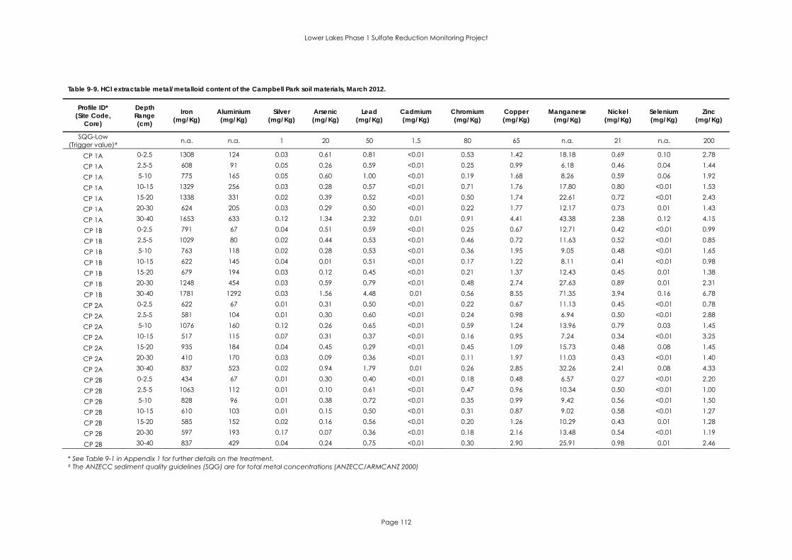
Lower Lakes Phase 1 Sulfate Reduction Monitoring Project
Page 112
Table 9-9. HCl extractable metal/metalloid content of the Campbell Park soil materials, March 2012.
Profile ID* (Site Code,
Core)
Depth Range (cm)
Iron (mg/Kg)
Aluminium (mg/Kg)
Silver (mg/Kg)
Arsenic (mg/Kg)
Lead (mg/Kg)
Cadmium (mg/Kg)
Chromium (mg/Kg)
Copper (mg/Kg)
Manganese (mg/Kg)
Nickel (mg/Kg)
Selenium (mg/Kg)
Zinc (mg/Kg)
SQG-Low (Trigger value)# n.a. n.a. 1 20 50 1.5 80 65 n.a. 21 n.a. 200
CP 1A 0-2.5 1308 124 0.03 0.61 0.81 <0.01 0.53 1.42 18.18 0.69 0.10 2.78
CP 1A 2.5-5 608 91 0.05 0.26 0.59 <0.01 0.25 0.99 6.18 0.46 0.04 1.44
CP 1A 5-10 775 165 0.05 0.60 1.00 <0.01 0.19 1.68 8.26 0.59 0.06 1.92
CP 1A 10-15 1329 256 0.03 0.28 0.57 <0.01 0.71 1.76 17.80 0.80 <0.01 1.53
CP 1A 15-20 1338 331 0.02 0.39 0.52 <0.01 0.50 1.74 22.61 0.72 <0.01 2.43
CP 1A 20-30 624 205 0.03 0.29 0.50 <0.01 0.22 1.77 12.17 0.73 0.01 1.43
CP 1A 30-40 1653 633 0.12 1.34 2.32 0.01 0.91 4.41 43.38 2.38 0.12 4.15
CP 1B 0-2.5 791 67 0.04 0.51 0.59 <0.01 0.25 0.67 12.71 0.42 <0.01 0.99
CP 1B 2.5-5 1029 80 0.02 0.44 0.53 <0.01 0.46 0.72 11.63 0.52 <0.01 0.85
CP 1B 5-10 763 118 0.02 0.28 0.53 <0.01 0.36 1.95 9.05 0.48 <0.01 1.65
CP 1B 10-15 622 145 0.04 0.01 0.51 <0.01 0.17 1.22 8.11 0.41 <0.01 0.98
CP 1B 15-20 679 194 0.03 0.12 0.45 <0.01 0.21 1.37 12.43 0.45 0.01 1.38
CP 1B 20-30 1248 454 0.03 0.59 0.79 <0.01 0.48 2.74 27.63 0.89 0.01 2.31
CP 1B 30-40 1781 1292 0.03 1.56 4.48 0.01 0.56 8.55 71.35 3.94 0.16 6.78
CP 2A 0-2.5 622 67 0.01 0.31 0.50 <0.01 0.22 0.67 11.13 0.45 <0.01 0.78
CP 2A 2.5-5 581 104 0.01 0.30 0.60 <0.01 0.24 0.98 6.94 0.50 <0.01 2.88
CP 2A 5-10 1076 160 0.12 0.26 0.65 <0.01 0.59 1.24 13.96 0.79 0.03 1.45
CP 2A 10-15 517 115 0.07 0.31 0.37 <0.01 0.16 0.95 7.24 0.34 <0.01 3.25
CP 2A 15-20 935 184 0.04 0.45 0.29 <0.01 0.45 1.09 15.73 0.48 0.08 1.45
CP 2A 20-30 410 170 0.03 0.09 0.36 <0.01 0.11 1.97 11.03 0.43 <0.01 1.40
CP 2A 30-40 837 523 0.02 0.94 1.79 0.01 0.26 2.85 32.26 2.41 0.08 4.33
CP 2B 0-2.5 434 67 0.01 0.30 0.40 <0.01 0.18 0.48 6.57 0.27 <0.01 2.20
CP 2B 2.5-5 1063 112 0.01 0.10 0.61 <0.01 0.47 0.96 10.34 0.50 <0.01 1.00
CP 2B 5-10 828 96 0.01 0.38 0.72 <0.01 0.35 0.99 9.42 0.56 <0.01 1.50
CP 2B 10-15 610 103 0.01 0.15 0.50 <0.01 0.31 0.87 9.02 0.58 <0.01 1.27
CP 2B 15-20 585 152 0.02 0.16 0.56 <0.01 0.20 1.26 10.29 0.43 0.01 1.28
CP 2B 20-30 597 193 0.17 0.07 0.36 <0.01 0.18 2.16 13.48 0.54 <0.01 1.19
CP 2B 30-40 837 429 0.04 0.24 0.75 <0.01 0.30 2.90 25.91 0.98 0.01 2.46
* See Table 9-1 in Appendix 1 for further details on the treatment. # The ANZECC sediment quality guidelines (SQG) are for total metal concentrations (ANZECC/ARMCANZ 2000)

Page 113
APPENDIX 3. Data for sulfate reduction rate samples

Page 114
Table 9-10. Mean total sulfate reduction rates for Waltowa in March 2012 (in units of nmol/g/day).
Treatment Sample Depth (cm) Rep 1 Rep 2 Rep 3 Av. S.D. 1A 0 - 2.5 41.050 31.788 0.000 24.279 21.530 2A 2.5 - 5 1.002 0.000 1.206 0.736 0.645 3A 5 - 10 0.000 0.000 0.000 0.000 0.000 4A 10 - 15 0.000 0.000 0.000 0.000 0.000 5A 15 - 20 0.000 0.000 0.000 0.000 0.000 6A 20 - 30 0.000 0.000 0.000 0.000 0.000 7A 30 - 40 0.000 0.000 0.000 0.000 0.000 1B 0 - 2.5 0.422 0.000 0.000 0.141 0.244 2B 2.5 - 5 34.321 1.659 1.165 12.381 19.001 3B 5 - 10 0.000 0.000 0.000 0.000 0.000 4B 10 - 15 0.000 0.000 0.000 0.000 0.000 5B 15 - 20 0.000 0.000 0.000 0.000 0.000 6B 20 - 30 0.000 0.000 0.000 0.000 0.000
Established Cotula
7B 30 - 40 0.000 0.000 0.000 0.000 0.000 1A 0 - 2.5 21.344 14.191 33.248 22.928 9.627 2A 2.5 - 5 19.662 11.299 54.733 28.565 23.045 3A 5 - 10 0.000 0.000 0.000 0.000 0.000 4A 10 - 15 0.000 0.000 0.000 0.000 0.000 5A 15 - 20 0.000 0.000 0.000 0.000 0.000 6A 20 - 30 0.000 0.000 0.000 0.000 0.000 7A 30 - 40 0.000 0.000 0.000 0.000 0.000 1B 0 - 2.5 0.000 0.000 0.000 0.000 0.000 2B 2.5 - 5 0.000 0.000 0.000 0.000 0.000 3B 5 - 10 0.000 1.739 0.937 0.892 0.870 4B 10 - 15 0.000 0.000 0.000 0.000 0.000 5B 15 - 20 0.000 0.000 0.000 0.000 0.000 6B 20 - 30 0.000 0.000 0.000 0.000 0.000
Established Juncus
7B 30 - 40 0.000 0.000 0.000 0.000 0.000 1A 0 - 2.5 1118.890 960.591 673.004 917.495 226.045 2A 2.5 - 5 1224.204 102.524 196.512 507.747 622.248 3A 5 - 10 4.612 0.000 2.383 2.332 2.307 4A 10 - 15 0.000 0.000 0.000 0.000 0.000 5A 15 - 20 0.000 0.000 0.000 0.000 0.000 6A 20 - 30 0.000 0.000 0.000 0.000 0.000 7A 30 - 40 0.000 0.000 0.000 0.000 0.000 1B 0 - 2.5 896.281 304.726 279.578 493.528 349.020 2B 2.5 - 5 87.276 22.568 121.059 76.968 50.048 3B 5 - 10 100.566 101.193 48.796 83.518 30.072 4B 10 - 15 n.a. 141.277 161.160 151.219 14.059 5B 15 - 20 43.518 461.699 69.086 191.434 234.405 6B 20 - 30 0.000 0.000 0.000 0.000 0.000
Established Phragmites
7B 30 - 40 0.000 0.000 0.000 0.000 0.000
Note: Values shown as 0.000 are less than the method detection limit.
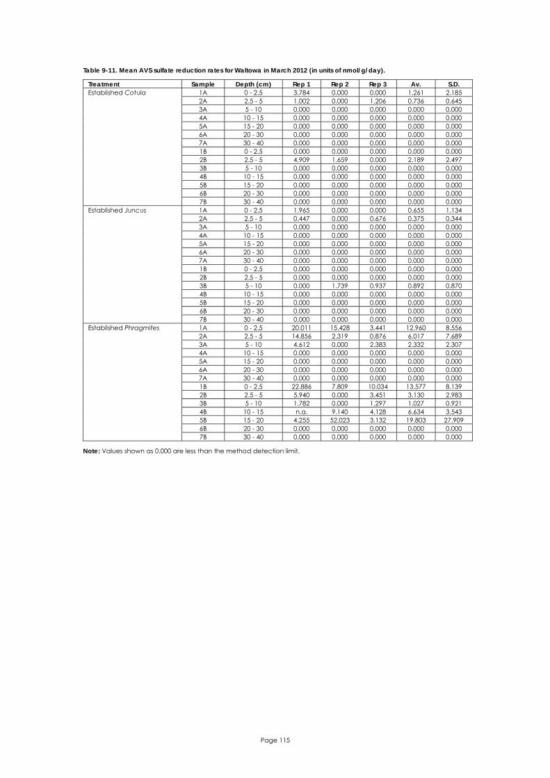
Page 115
Table 9-11. Mean AVS sulfate reduction rates for Waltowa in March 2012 (in units of nmol/g/day).
Treatment Sample Depth (cm) Rep 1 Rep 2 Rep 3 Av. S.D. 1A 0 - 2.5 3.784 0.000 0.000 1.261 2.185 2A 2.5 - 5 1.002 0.000 1.206 0.736 0.645 3A 5 - 10 0.000 0.000 0.000 0.000 0.000 4A 10 - 15 0.000 0.000 0.000 0.000 0.000 5A 15 - 20 0.000 0.000 0.000 0.000 0.000 6A 20 - 30 0.000 0.000 0.000 0.000 0.000 7A 30 - 40 0.000 0.000 0.000 0.000 0.000 1B 0 - 2.5 0.000 0.000 0.000 0.000 0.000 2B 2.5 - 5 4.909 1.659 0.000 2.189 2.497 3B 5 - 10 0.000 0.000 0.000 0.000 0.000 4B 10 - 15 0.000 0.000 0.000 0.000 0.000 5B 15 - 20 0.000 0.000 0.000 0.000 0.000 6B 20 - 30 0.000 0.000 0.000 0.000 0.000
Established Cotula
7B 30 - 40 0.000 0.000 0.000 0.000 0.000 1A 0 - 2.5 1.965 0.000 0.000 0.655 1.134 2A 2.5 - 5 0.447 0.000 0.676 0.375 0.344 3A 5 - 10 0.000 0.000 0.000 0.000 0.000 4A 10 - 15 0.000 0.000 0.000 0.000 0.000 5A 15 - 20 0.000 0.000 0.000 0.000 0.000 6A 20 - 30 0.000 0.000 0.000 0.000 0.000 7A 30 - 40 0.000 0.000 0.000 0.000 0.000 1B 0 - 2.5 0.000 0.000 0.000 0.000 0.000 2B 2.5 - 5 0.000 0.000 0.000 0.000 0.000 3B 5 - 10 0.000 1.739 0.937 0.892 0.870 4B 10 - 15 0.000 0.000 0.000 0.000 0.000 5B 15 - 20 0.000 0.000 0.000 0.000 0.000 6B 20 - 30 0.000 0.000 0.000 0.000 0.000
Established Juncus
7B 30 - 40 0.000 0.000 0.000 0.000 0.000 1A 0 - 2.5 20.011 15.428 3.441 12.960 8.556 2A 2.5 - 5 14.856 2.319 0.876 6.017 7.689 3A 5 - 10 4.612 0.000 2.383 2.332 2.307 4A 10 - 15 0.000 0.000 0.000 0.000 0.000 5A 15 - 20 0.000 0.000 0.000 0.000 0.000 6A 20 - 30 0.000 0.000 0.000 0.000 0.000 7A 30 - 40 0.000 0.000 0.000 0.000 0.000 1B 0 - 2.5 22.886 7.809 10.034 13.577 8.139 2B 2.5 - 5 5.940 0.000 3.451 3.130 2.983 3B 5 - 10 1.782 0.000 1.297 1.027 0.921 4B 10 - 15 n.a. 9.140 4.128 6.634 3.543 5B 15 - 20 4.255 52.023 3.132 19.803 27.909 6B 20 - 30 0.000 0.000 0.000 0.000 0.000
Established Phragmites
7B 30 - 40 0.000 0.000 0.000 0.000 0.000
Note: Values shown as 0.000 are less than the method detection limit.

Page 116
Table 9-12. Mean S0 sulfate reduction rates for Waltowa in March 2012 (in units of nmol/g/day).
Treatment Sample Depth (cm) Rep 1 Rep 2 Rep 3 Av. S.D. 1A 0 - 2.5 36.534 31.081 0.000 22.538 19.708 2A 2.5 - 5 0.000 0.000 0.000 0.000 0.000 3A 5 - 10 0.000 0.000 0.000 0.000 0.000 4A 10 - 15 0.000 0.000 0.000 0.000 0.000 5A 15 - 20 0.000 0.000 0.000 0.000 0.000 6A 20 - 30 0.000 0.000 0.000 0.000 0.000 7A 30 - 40 0.000 0.000 0.000 0.000 0.000 1B 0 - 2.5 0.000 0.000 0.000 0.000 0.000 2B 2.5 - 5 28.846 0.000 0.000 9.615 16.654 3B 5 - 10 0.000 0.000 0.000 0.000 0.000 4B 10 - 15 0.000 0.000 0.000 0.000 0.000 5B 15 - 20 0.000 0.000 0.000 0.000 0.000 6B 20 - 30 0.000 0.000 0.000 0.000 0.000
Established Cotula
7B 30 - 40 0.000 0.000 0.000 0.000 0.000 1A 0 - 2.5 19.047 13.888 32.671 21.869 9.704 2A 2.5 - 5 18.828 10.876 52.757 27.487 22.243 3A 5 - 10 0.000 0.000 0.000 0.000 0.000 4A 10 - 15 0.000 0.000 0.000 0.000 0.000 5A 15 - 20 0.000 0.000 0.000 0.000 0.000 6A 20 - 30 0.000 0.000 0.000 0.000 0.000 7A 30 - 40 0.000 0.000 0.000 0.000 0.000 1B 0 - 2.5 0.000 0.000 0.000 0.000 0.000 2B 2.5 - 5 0.000 0.000 0.000 0.000 0.000 3B 5 - 10 0.000 0.000 0.000 0.000 0.000 4B 10 - 15 0.000 0.000 0.000 0.000 0.000 5B 15 - 20 0.000 0.000 0.000 0.000 0.000 6B 20 - 30 0.000 0.000 0.000 0.000 0.000
Established Juncus
7B 30 - 40 0.000 0.000 0.000 0.000 0.000 1A 0 - 2.5 1092.260 931.399 660.804 894.821 218.042 2A 2.5 - 5 1200.026 98.143 193.905 497.358 610.409 3A 5 - 10 0.000 0.000 0.000 0.000 0.000 4A 10 - 15 0.000 0.000 0.000 0.000 0.000 5A 15 - 20 0.000 0.000 0.000 0.000 0.000 6A 20 - 30 0.000 0.000 0.000 0.000 0.000 7A 30 - 40 0.000 0.000 0.000 0.000 0.000 1B 0 - 2.5 829.801 283.746 260.582 458.043 322.160 2B 2.5 - 5 78.483 21.895 114.989 71.789 46.907 3B 5 - 10 96.943 97.890 45.747 80.193 29.835 4B 10 - 15 n.a. 128.563 153.800 141.182 17.846 5B 15 - 20 39.263 406.555 65.954 170.591 204.787 6B 20 - 30 0.000 0.000 0.000 0.000 0.000
Established Phragmites
7B 30 - 40 0.000 0.000 0.000 0.000 0.000
Note: Values shown as 0.000 are less than the method detection limit.

Page 117
Table 9-13. Mean pyrite sulfate reduction rates for Waltowa in March 2012 (in units of nmol/g/day).
Treatment Sample Depth (cm) Rep 1 Rep 2 Rep 3 Av. S.D. 1A 0 - 2.5 0.732 0.707 0.000 0.480 0.416 2A 2.5 - 5 0.000 0.000 0.000 0.000 0.000 3A 5 - 10 0.000 0.000 0.000 0.000 0.000 4A 10 - 15 0.000 0.000 0.000 0.000 0.000 5A 15 - 20 0.000 0.000 0.000 0.000 0.000 6A 20 - 30 0.000 0.000 0.000 0.000 0.000 7A 30 - 40 0.000 0.000 0.000 0.000 0.000 1B 0 - 2.5 0.422 0.000 0.000 0.141 0.244 2B 2.5 - 5 0.566 0.000 1.165 0.577 0.583 3B 5 - 10 0.000 0.000 0.000 0.000 0.000 4B 10 - 15 0.000 0.000 0.000 0.000 0.000 5B 15 - 20 0.000 0.000 0.000 0.000 0.000 6B 20 - 30 0.000 0.000 0.000 0.000 0.000
Established Cotula
7B 30 - 40 0.000 0.000 0.000 0.000 0.000 1A 0 - 2.5 0.332 0.302 0.577 0.404 0.151 2A 2.5 - 5 0.388 0.423 1.300 0.704 0.517 3A 5 - 10 0.000 0.000 0.000 0.000 0.000 4A 10 - 15 0.000 0.000 0.000 0.000 0.000 5A 15 - 20 0.000 0.000 0.000 0.000 0.000 6A 20 - 30 0.000 0.000 0.000 0.000 0.000 7A 30 - 40 0.000 0.000 0.000 0.000 0.000 1B 0 - 2.5 0.000 0.000 0.000 0.000 0.000 2B 2.5 - 5 0.000 0.000 0.000 0.000 0.000 3B 5 - 10 0.000 0.000 0.000 0.000 0.000 4B 10 - 15 0.000 0.000 0.000 0.000 0.000 5B 15 - 20 0.000 0.000 0.000 0.000 0.000 6B 20 - 30 0.000 0.000 0.000 0.000 0.000
Established Juncus
7B 30 - 40 0.000 0.000 0.000 0.000 0.000 1A 0 - 2.5 6.619 13.765 8.759 9.714 3.667 2A 2.5 - 5 9.323 2.062 1.731 4.372 4.291 3A 5 - 10 0.000 0.000 0.000 0.000 0.000 4A 10 - 15 0.000 0.000 0.000 0.000 0.000 5A 15 - 20 0.000 0.000 0.000 0.000 0.000 6A 20 - 30 0.000 0.000 0.000 0.000 0.000 7A 30 - 40 0.000 0.000 0.000 0.000 0.000 1B 0 - 2.5 43.593 13.170 8.963 21.909 18.897 2B 2.5 - 5 2.853 0.673 2.620 2.049 1.197 3B 5 - 10 1.841 3.303 1.752 2.299 0.871 4B 10 - 15 n.a. 3.575 3.231 3.403 0.243 5B 15 - 20 0.000 3.120 0.000 1.040 1.802 6B 20 - 30 0.000 0.000 0.000 0.000 0.000
Established Phragmites
7B 30 - 40 0.000 0.000 0.000 0.000 0.000
Note: Values shown as 0.000 are less than the method detection limit.
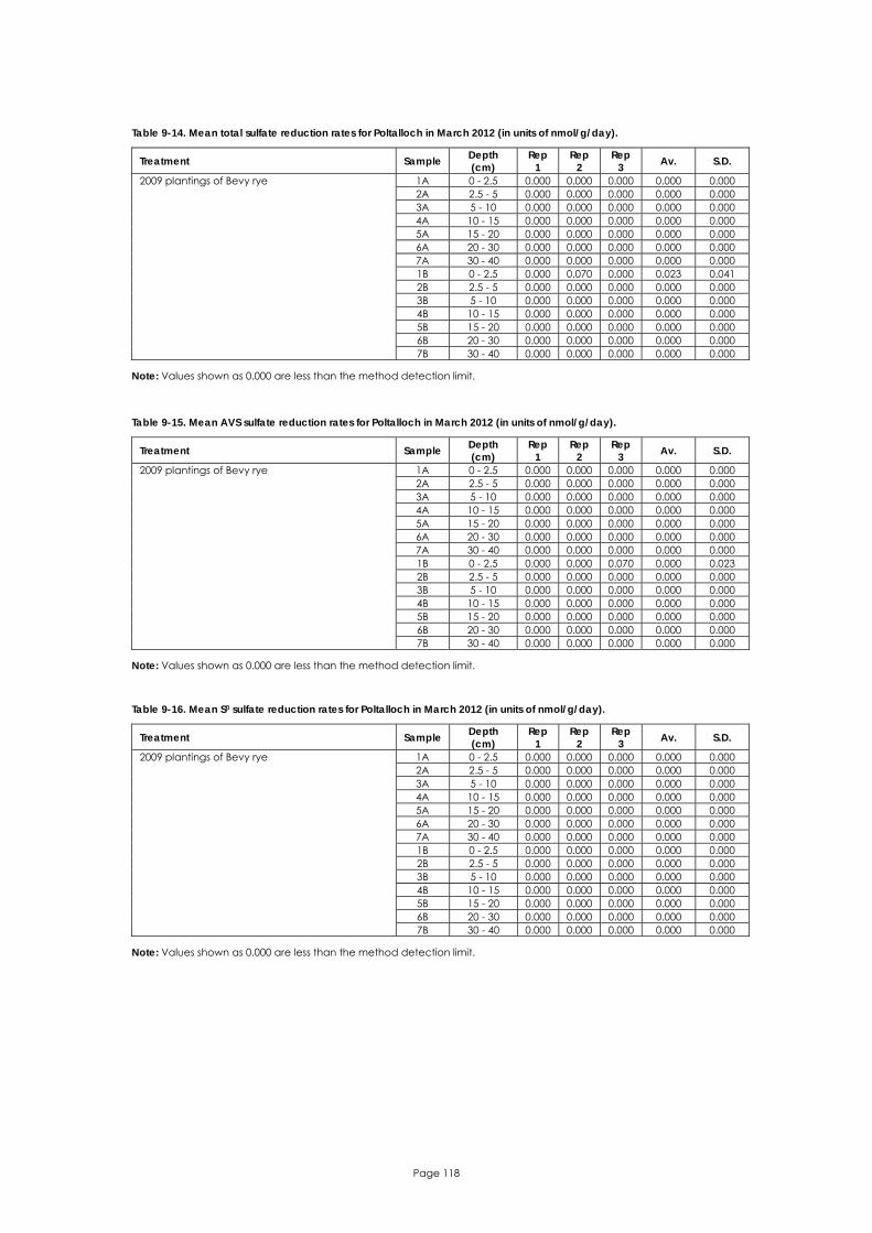
Page 118
Table 9-14. Mean total sulfate reduction rates for Poltalloch in March 2012 (in units of nmol/g/day).
Treatment Sample Depth (cm)
Rep 1
Rep 2
Rep 3 Av. S.D.
1A 0 - 2.5 0.000 0.000 0.000 0.000 0.000 2A 2.5 - 5 0.000 0.000 0.000 0.000 0.000 3A 5 - 10 0.000 0.000 0.000 0.000 0.000 4A 10 - 15 0.000 0.000 0.000 0.000 0.000 5A 15 - 20 0.000 0.000 0.000 0.000 0.000 6A 20 - 30 0.000 0.000 0.000 0.000 0.000 7A 30 - 40 0.000 0.000 0.000 0.000 0.000 1B 0 - 2.5 0.000 0.070 0.000 0.023 0.041 2B 2.5 - 5 0.000 0.000 0.000 0.000 0.000 3B 5 - 10 0.000 0.000 0.000 0.000 0.000 4B 10 - 15 0.000 0.000 0.000 0.000 0.000 5B 15 - 20 0.000 0.000 0.000 0.000 0.000 6B 20 - 30 0.000 0.000 0.000 0.000 0.000
2009 plantings of Bevy rye
7B 30 - 40 0.000 0.000 0.000 0.000 0.000
Note: Values shown as 0.000 are less than the method detection limit. Table 9-15. Mean AVS sulfate reduction rates for Poltalloch in March 2012 (in units of nmol/g/day).
Treatment Sample Depth (cm)
Rep 1
Rep 2
Rep 3 Av. S.D.
1A 0 - 2.5 0.000 0.000 0.000 0.000 0.000 2A 2.5 - 5 0.000 0.000 0.000 0.000 0.000 3A 5 - 10 0.000 0.000 0.000 0.000 0.000 4A 10 - 15 0.000 0.000 0.000 0.000 0.000 5A 15 - 20 0.000 0.000 0.000 0.000 0.000 6A 20 - 30 0.000 0.000 0.000 0.000 0.000 7A 30 - 40 0.000 0.000 0.000 0.000 0.000 1B 0 - 2.5 0.000 0.000 0.070 0.000 0.023 2B 2.5 - 5 0.000 0.000 0.000 0.000 0.000 3B 5 - 10 0.000 0.000 0.000 0.000 0.000 4B 10 - 15 0.000 0.000 0.000 0.000 0.000 5B 15 - 20 0.000 0.000 0.000 0.000 0.000 6B 20 - 30 0.000 0.000 0.000 0.000 0.000
2009 plantings of Bevy rye
7B 30 - 40 0.000 0.000 0.000 0.000 0.000
Note: Values shown as 0.000 are less than the method detection limit. Table 9-16. Mean S0 sulfate reduction rates for Poltalloch in March 2012 (in units of nmol/g/day).
Treatment Sample Depth (cm)
Rep 1
Rep 2
Rep 3 Av. S.D.
1A 0 - 2.5 0.000 0.000 0.000 0.000 0.000 2A 2.5 - 5 0.000 0.000 0.000 0.000 0.000 3A 5 - 10 0.000 0.000 0.000 0.000 0.000 4A 10 - 15 0.000 0.000 0.000 0.000 0.000 5A 15 - 20 0.000 0.000 0.000 0.000 0.000 6A 20 - 30 0.000 0.000 0.000 0.000 0.000 7A 30 - 40 0.000 0.000 0.000 0.000 0.000 1B 0 - 2.5 0.000 0.000 0.000 0.000 0.000 2B 2.5 - 5 0.000 0.000 0.000 0.000 0.000 3B 5 - 10 0.000 0.000 0.000 0.000 0.000 4B 10 - 15 0.000 0.000 0.000 0.000 0.000 5B 15 - 20 0.000 0.000 0.000 0.000 0.000 6B 20 - 30 0.000 0.000 0.000 0.000 0.000
2009 plantings of Bevy rye
7B 30 - 40 0.000 0.000 0.000 0.000 0.000
Note: Values shown as 0.000 are less than the method detection limit.

Page 119
Table 9-17. Mean pyrite sulfate reduction rates for Poltalloch in March 2012 (in units of nmol/g/day).
Treatment Sample Depth (cm)
Rep 1
Rep 2
Rep 3 Av. S.D.
1A 0 - 2.5 0.000 0.000 0.000 0.000 0.000 2A 2.5 - 5 0.000 0.000 0.000 0.000 0.000 3A 5 - 10 0.000 0.000 0.000 0.000 0.000 4A 10 - 15 0.000 0.000 0.000 0.000 0.000 5A 15 - 20 0.000 0.000 0.000 0.000 0.000 6A 20 - 30 0.000 0.000 0.000 0.000 0.000 7A 30 - 40 0.000 0.000 0.000 0.000 0.000 1B 0 - 2.5 0.000 0.000 0.000 0.000 0.000 2B 2.5 - 5 0.000 0.000 0.000 0.000 0.000 3B 5 - 10 0.000 0.000 0.000 0.000 0.000 4B 10 - 15 0.000 0.000 0.000 0.000 0.000 5B 15 - 20 0.000 0.000 0.000 0.000 0.000 6B 20 - 30 0.000 0.000 0.000 0.000 0.000
2009 plantings of Bevy rye
7B 30 - 40 0.000 0.000 0.000 0.000 0.000
Note: Values shown as 0.000 are less than the method detection limit. Table 9-18. Mean total sulfate reduction rates for Tolderol in March 2012 (in units of nmol/g/day).
Treatment Sample Depth (cm) Rep 1 Rep 2 Rep 3 Av. S.D.
1A 0 - 2.5 0.000 0.000 0.000 0.000 0.000 2A 2.5 - 5 0.000 0.000 0.000 0.000 0.000 3A 5 - 10 0.000 0.000 0.000 0.000 0.000 4A 10 - 15 0.000 0.000 0.000 0.000 0.000 5A 15 - 20 0.000 0.000 0.000 0.000 0.000 6A 20 - 30 0.000 0.000 0.000 0.000 0.000 7A 30 - 40 0.000 0.000 0.000 0.000 0.000 1B 0 - 2.5 0.000 0.000 0.000 0.000 0.000 2B 2.5 - 5 0.000 0.000 0.000 0.000 0.000 3B 5 - 10 7.979 0.324 0.000 2.768 4.516 4B 10 - 15 0.000 0.000 0.000 0.000 0.000 5B 15 - 20 0.000 0.000 0.000 0.000 0.000 6B 20 - 30 0.000 0.000 0.000 0.000 0.000
Scald (no bioremediation)
7B 30 - 40 0.000 0.000 0.000 0.000 0.000 1A 0 - 2.5 0.000 0.000 0.000 0.000 0.000 2A 2.5 - 5 0.000 0.249 0.000 0.083 0.144 3A 5 - 10 0.000 0.000 0.000 0.000 0.000 4A 10 - 15 0.000 0.000 0.000 0.000 0.000 5A 15 - 20 0.000 0.000 0.000 0.000 0.000 6A 20 - 30 0.000 0.000 0.000 0.000 0.000 7A 30 - 40 0.000 0.000 0.000 0.000 0.000 1B 0 - 2.5 0.000 0.000 0.000 0.000 0.000 2B 2.5 - 5 0.000 0.000 0.000 0.000 0.000 3B 5 - 10 0.000 0.000 0.000 0.000 0.000 4B 10 - 15 0.000 0.000 0.000 0.000 0.000 5B 15 - 20 0.000 0.000 0.000 0.000 0.000 6B 20 - 30 0.000 0.000 0.000 0.000 0.000
2010 planted Juncus into 2009 plantings of Bevy rye
7B 30 - 40 0.000 0.000 0.000 0.000 0.000
Note: Values shown as 0.000 are less than the method detection limit.

Page 120
Table 9-19. Mean AVS sulfate reduction rates for Tolderol in March 2012 (in units of nmol/g/day).
Treatment Sample Depth (cm) Rep 1 Rep 2 Rep 3 Av. S.D.
1A 0 - 2.5 0.000 0.000 0.000 0.000 0.000 2A 2.5 - 5 0.000 0.000 0.000 0.000 0.000 3A 5 - 10 0.000 0.000 0.000 0.000 0.000 4A 10 - 15 0.000 0.000 0.000 0.000 0.000 5A 15 - 20 0.000 0.000 0.000 0.000 0.000 6A 20 - 30 0.000 0.000 0.000 0.000 0.000 7A 30 - 40 0.000 0.000 0.000 0.000 0.000 1B 0 - 2.5 0.000 0.000 0.000 0.000 0.000 2B 2.5 - 5 0.000 0.000 0.000 0.000 0.000 3B 5 - 10 0.662 0.324 0.000 0.328 0.331 4B 10 - 15 0.000 0.000 0.000 0.000 0.000 5B 15 - 20 0.000 0.000 0.000 0.000 0.000 6B 20 - 30 0.000 0.000 0.000 0.000 0.000
Scald (no bioremediation)
7B 30 - 40 0.000 0.000 0.000 0.000 0.000 1A 0 - 2.5 0.000 0.000 0.000 0.000 0.000 2A 2.5 - 5 0.000 0.249 0.000 0.083 0.144 3A 5 - 10 0.000 0.000 0.000 0.000 0.000 4A 10 - 15 0.000 0.000 0.000 0.000 0.000 5A 15 - 20 0.000 0.000 0.000 0.000 0.000 6A 20 - 30 0.000 0.000 0.000 0.000 0.000 7A 30 - 40 0.000 0.000 0.000 0.000 0.000 1B 0 - 2.5 0.000 0.000 0.000 0.000 0.000 2B 2.5 - 5 0.000 0.000 0.000 0.000 0.000 3B 5 - 10 0.000 0.000 0.000 0.000 0.000 4B 10 - 15 0.000 0.000 0.000 0.000 0.000 5B 15 - 20 0.000 0.000 0.000 0.000 0.000 6B 20 - 30 0.000 0.000 0.000 0.000 0.000
2010 planted Juncus into 2009 plantings of Bevy rye
7B 30 - 40 0.000 0.000 0.000 0.000 0.000
Note: Values shown as 0.000 are less than the method detection limit. Table 9-20. Mean S0 sulfate reduction rates for Tolderol in March 2012 (in units of nmol/g/day).
Treatment Sample Depth (cm)
Rep 1
Rep 2
Rep 3 Av. S.D.
1A 0 - 2.5 0.000 0.000 0.000 0.000 0.000 2A 2.5 - 5 0.000 0.000 0.000 0.000 0.000 3A 5 - 10 0.000 0.000 0.000 0.000 0.000 4A 10 - 15 0.000 0.000 0.000 0.000 0.000 5A 15 - 20 0.000 0.000 0.000 0.000 0.000 6A 20 - 30 0.000 0.000 0.000 0.000 0.000 7A 30 - 40 0.000 0.000 0.000 0.000 0.000 1B 0 - 2.5 0.000 0.000 0.000 0.000 0.000 2B 2.5 - 5 0.000 0.000 0.000 0.000 0.000 3B 5 - 10 7.317 0.000 0.000 2.439 4.225 4B 10 - 15 0.000 0.000 0.000 0.000 0.000 5B 15 - 20 0.000 0.000 0.000 0.000 0.000 6B 20 - 30 0.000 0.000 0.000 0.000 0.000
Scald (no bioremediation)
7B 30 - 40 0.000 0.000 0.000 0.000 0.000 1A 0 - 2.5 0.000 0.000 0.000 0.000 0.000 2A 2.5 - 5 0.000 0.000 0.000 0.000 0.000 3A 5 - 10 0.000 0.000 0.000 0.000 0.000 4A 10 - 15 0.000 0.000 0.000 0.000 0.000 5A 15 - 20 0.000 0.000 0.000 0.000 0.000 6A 20 - 30 0.000 0.000 0.000 0.000 0.000 7A 30 - 40 0.000 0.000 0.000 0.000 0.000 1B 0 - 2.5 0.000 0.000 0.000 0.000 0.000 2B 2.5 - 5 0.000 0.000 0.000 0.000 0.000 3B 5 - 10 0.000 0.000 0.000 0.000 0.000 4B 10 - 15 0.000 0.000 0.000 0.000 0.000 5B 15 - 20 0.000 0.000 0.000 0.000 0.000 6B 20 - 30 0.000 0.000 0.000 0.000 0.000
2010 planted Juncus into 2009 plantings of Bevy rye
7B 30 - 40 0.000 0.000 0.000 0.000 0.000
Note: Values shown as 0.000 are less than the method detection limit.
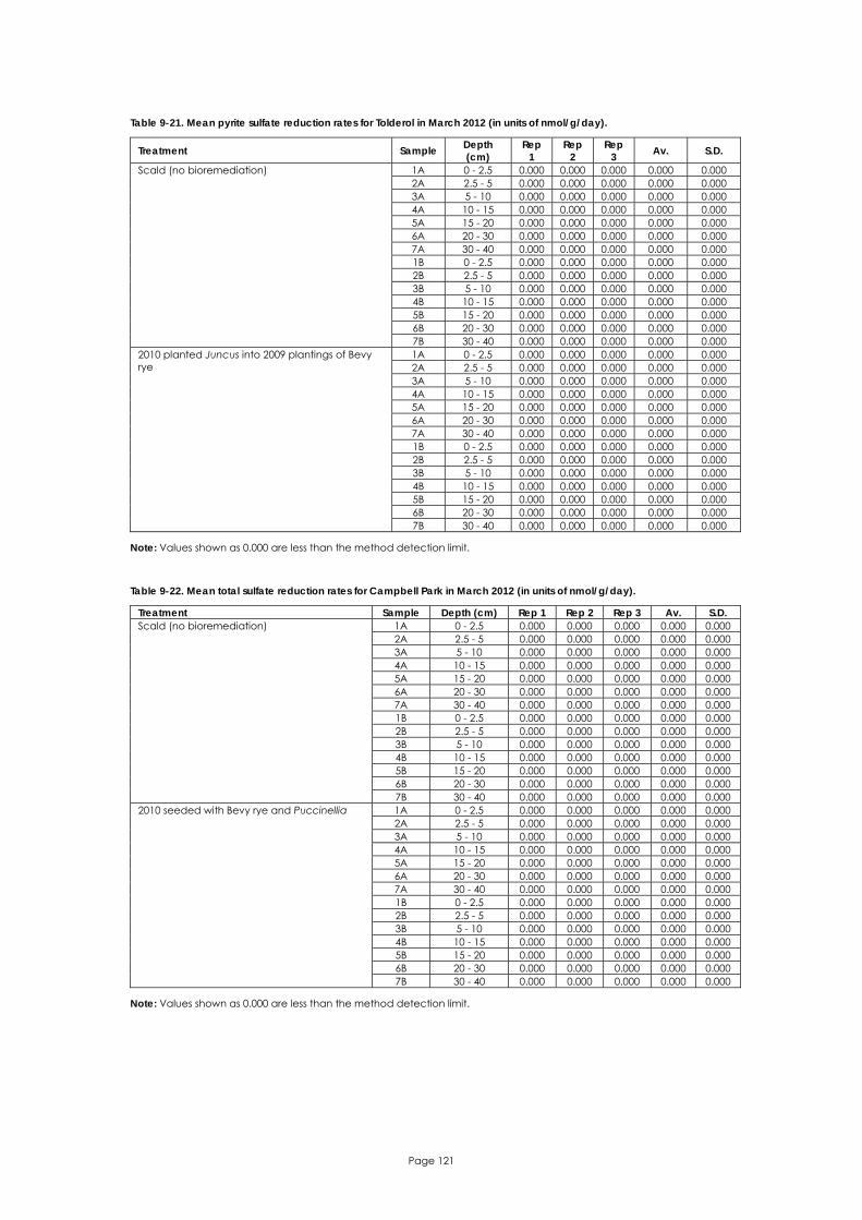
Page 121
Table 9-21. Mean pyrite sulfate reduction rates for Tolderol in March 2012 (in units of nmol/g/day).
Treatment Sample Depth (cm)
Rep 1
Rep 2
Rep 3 Av. S.D.
1A 0 - 2.5 0.000 0.000 0.000 0.000 0.000 2A 2.5 - 5 0.000 0.000 0.000 0.000 0.000 3A 5 - 10 0.000 0.000 0.000 0.000 0.000 4A 10 - 15 0.000 0.000 0.000 0.000 0.000 5A 15 - 20 0.000 0.000 0.000 0.000 0.000 6A 20 - 30 0.000 0.000 0.000 0.000 0.000 7A 30 - 40 0.000 0.000 0.000 0.000 0.000 1B 0 - 2.5 0.000 0.000 0.000 0.000 0.000 2B 2.5 - 5 0.000 0.000 0.000 0.000 0.000 3B 5 - 10 0.000 0.000 0.000 0.000 0.000 4B 10 - 15 0.000 0.000 0.000 0.000 0.000 5B 15 - 20 0.000 0.000 0.000 0.000 0.000 6B 20 - 30 0.000 0.000 0.000 0.000 0.000
Scald (no bioremediation)
7B 30 - 40 0.000 0.000 0.000 0.000 0.000 1A 0 - 2.5 0.000 0.000 0.000 0.000 0.000 2A 2.5 - 5 0.000 0.000 0.000 0.000 0.000 3A 5 - 10 0.000 0.000 0.000 0.000 0.000 4A 10 - 15 0.000 0.000 0.000 0.000 0.000 5A 15 - 20 0.000 0.000 0.000 0.000 0.000 6A 20 - 30 0.000 0.000 0.000 0.000 0.000 7A 30 - 40 0.000 0.000 0.000 0.000 0.000 1B 0 - 2.5 0.000 0.000 0.000 0.000 0.000 2B 2.5 - 5 0.000 0.000 0.000 0.000 0.000 3B 5 - 10 0.000 0.000 0.000 0.000 0.000 4B 10 - 15 0.000 0.000 0.000 0.000 0.000 5B 15 - 20 0.000 0.000 0.000 0.000 0.000 6B 20 - 30 0.000 0.000 0.000 0.000 0.000
2010 planted Juncus into 2009 plantings of Bevy rye
7B 30 - 40 0.000 0.000 0.000 0.000 0.000
Note: Values shown as 0.000 are less than the method detection limit. Table 9-22. Mean total sulfate reduction rates for Campbell Park in March 2012 (in units of nmol/g/day).
Treatment Sample Depth (cm) Rep 1 Rep 2 Rep 3 Av. S.D. 1A 0 - 2.5 0.000 0.000 0.000 0.000 0.000 2A 2.5 - 5 0.000 0.000 0.000 0.000 0.000 3A 5 - 10 0.000 0.000 0.000 0.000 0.000 4A 10 - 15 0.000 0.000 0.000 0.000 0.000 5A 15 - 20 0.000 0.000 0.000 0.000 0.000 6A 20 - 30 0.000 0.000 0.000 0.000 0.000 7A 30 - 40 0.000 0.000 0.000 0.000 0.000 1B 0 - 2.5 0.000 0.000 0.000 0.000 0.000 2B 2.5 - 5 0.000 0.000 0.000 0.000 0.000 3B 5 - 10 0.000 0.000 0.000 0.000 0.000 4B 10 - 15 0.000 0.000 0.000 0.000 0.000 5B 15 - 20 0.000 0.000 0.000 0.000 0.000 6B 20 - 30 0.000 0.000 0.000 0.000 0.000
Scald (no bioremediation)
7B 30 - 40 0.000 0.000 0.000 0.000 0.000 1A 0 - 2.5 0.000 0.000 0.000 0.000 0.000 2A 2.5 - 5 0.000 0.000 0.000 0.000 0.000 3A 5 - 10 0.000 0.000 0.000 0.000 0.000 4A 10 - 15 0.000 0.000 0.000 0.000 0.000 5A 15 - 20 0.000 0.000 0.000 0.000 0.000 6A 20 - 30 0.000 0.000 0.000 0.000 0.000 7A 30 - 40 0.000 0.000 0.000 0.000 0.000 1B 0 - 2.5 0.000 0.000 0.000 0.000 0.000 2B 2.5 - 5 0.000 0.000 0.000 0.000 0.000 3B 5 - 10 0.000 0.000 0.000 0.000 0.000 4B 10 - 15 0.000 0.000 0.000 0.000 0.000 5B 15 - 20 0.000 0.000 0.000 0.000 0.000 6B 20 - 30 0.000 0.000 0.000 0.000 0.000
2010 seeded with Bevy rye and Puccinellia
7B 30 - 40 0.000 0.000 0.000 0.000 0.000
Note: Values shown as 0.000 are less than the method detection limit.

Page 122
Table 9-23. Mean AVS sulfate reduction rates for Campbell Park in March 2012 (in units of nmol/g/day).
Treatment Sample Depth (cm) Rep 1 Rep 2 Rep 3 Av. S.D. 1A 0 - 2.5 0.000 0.000 0.000 0.000 0.000 2A 2.5 - 5 0.000 0.000 0.000 0.000 0.000 3A 5 - 10 0.000 0.000 0.000 0.000 0.000 4A 10 - 15 0.000 0.000 0.000 0.000 0.000 5A 15 - 20 0.000 0.000 0.000 0.000 0.000 6A 20 - 30 0.000 0.000 0.000 0.000 0.000 7A 30 - 40 0.000 0.000 0.000 0.000 0.000 1B 0 - 2.5 0.000 0.000 0.000 0.000 0.000 2B 2.5 - 5 0.000 0.000 0.000 0.000 0.000 3B 5 - 10 0.000 0.000 0.000 0.000 0.000 4B 10 - 15 0.000 0.000 0.000 0.000 0.000 5B 15 - 20 0.000 0.000 0.000 0.000 0.000 6B 20 - 30 0.000 0.000 0.000 0.000 0.000
Scald (no bioremediation)
7B 30 - 40 0.000 0.000 0.000 0.000 0.000 1A 0 - 2.5 0.000 0.000 0.000 0.000 0.000 2A 2.5 - 5 0.000 0.000 0.000 0.000 0.000 3A 5 - 10 0.000 0.000 0.000 0.000 0.000 4A 10 - 15 0.000 0.000 0.000 0.000 0.000 5A 15 - 20 0.000 0.000 0.000 0.000 0.000 6A 20 - 30 0.000 0.000 0.000 0.000 0.000 7A 30 - 40 0.000 0.000 0.000 0.000 0.000 1B 0 - 2.5 0.000 0.000 0.000 0.000 0.000 2B 2.5 - 5 0.000 0.000 0.000 0.000 0.000 3B 5 - 10 0.000 0.000 0.000 0.000 0.000 4B 10 - 15 0.000 0.000 0.000 0.000 0.000 5B 15 - 20 0.000 0.000 0.000 0.000 0.000 6B 20 - 30 0.000 0.000 0.000 0.000 0.000
2010 seeded with Bevy rye and Puccinellia
7B 30 - 40 0.000 0.000 0.000 0.000 0.000
Note: Values shown as 0.000 are less than the method detection limit. Table 9-24. Mean S0 sulfate reduction rates for Campbell Park March 2012 (in units of nmol/g/day).
Treatment Sample Depth (cm) Rep 1 Rep 2 Rep 3 Av. S.D. 1A 0 - 2.5 0.000 0.000 0.000 0.000 0.000 2A 2.5 - 5 0.000 0.000 0.000 0.000 0.000 3A 5 - 10 0.000 0.000 0.000 0.000 0.000 4A 10 - 15 0.000 0.000 0.000 0.000 0.000 5A 15 - 20 0.000 0.000 0.000 0.000 0.000 6A 20 - 30 0.000 0.000 0.000 0.000 0.000 7A 30 - 40 0.000 0.000 0.000 0.000 0.000 1B 0 - 2.5 0.000 0.000 0.000 0.000 0.000 2B 2.5 - 5 0.000 0.000 0.000 0.000 0.000 3B 5 - 10 0.000 0.000 0.000 0.000 0.000 4B 10 - 15 0.000 0.000 0.000 0.000 0.000 5B 15 - 20 0.000 0.000 0.000 0.000 0.000 6B 20 - 30 0.000 0.000 0.000 0.000 0.000
Scald (no bioremediation)
7B 30 - 40 0.000 0.000 0.000 0.000 0.000 1A 0 - 2.5 0.000 0.000 0.000 0.000 0.000 2A 2.5 - 5 0.000 0.000 0.000 0.000 0.000 3A 5 - 10 0.000 0.000 0.000 0.000 0.000 4A 10 - 15 0.000 0.000 0.000 0.000 0.000 5A 15 - 20 0.000 0.000 0.000 0.000 0.000 6A 20 - 30 0.000 0.000 0.000 0.000 0.000 7A 30 - 40 0.000 0.000 0.000 0.000 0.000 1B 0 - 2.5 0.000 0.000 0.000 0.000 0.000 2B 2.5 - 5 0.000 0.000 0.000 0.000 0.000 3B 5 - 10 0.000 0.000 0.000 0.000 0.000 4B 10 - 15 0.000 0.000 0.000 0.000 0.000 5B 15 - 20 0.000 0.000 0.000 0.000 0.000 6B 20 - 30 0.000 0.000 0.000 0.000 0.000
2010 seeded with Bevy rye and Puccinellia
7B 30 - 40 0.000 0.000 0.000 0.000 0.000
Note: Values shown as 0.000 are less than the method detection limit.
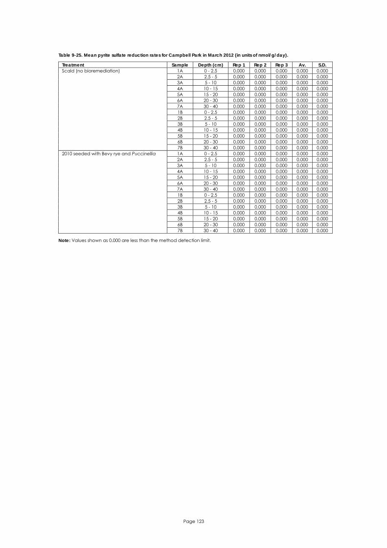
Page 123
Table 9-25. Mean pyrite sulfate reduction rates for Campbell Park in March 2012 (in units of nmol/g/day).
Treatment Sample Depth (cm) Rep 1 Rep 2 Rep 3 Av. S.D. 1A 0 - 2.5 0.000 0.000 0.000 0.000 0.000 2A 2.5 - 5 0.000 0.000 0.000 0.000 0.000 3A 5 - 10 0.000 0.000 0.000 0.000 0.000 4A 10 - 15 0.000 0.000 0.000 0.000 0.000 5A 15 - 20 0.000 0.000 0.000 0.000 0.000 6A 20 - 30 0.000 0.000 0.000 0.000 0.000 7A 30 - 40 0.000 0.000 0.000 0.000 0.000 1B 0 - 2.5 0.000 0.000 0.000 0.000 0.000 2B 2.5 - 5 0.000 0.000 0.000 0.000 0.000 3B 5 - 10 0.000 0.000 0.000 0.000 0.000 4B 10 - 15 0.000 0.000 0.000 0.000 0.000 5B 15 - 20 0.000 0.000 0.000 0.000 0.000 6B 20 - 30 0.000 0.000 0.000 0.000 0.000
Scald (no bioremediation)
7B 30 - 40 0.000 0.000 0.000 0.000 0.000 1A 0 - 2.5 0.000 0.000 0.000 0.000 0.000 2A 2.5 - 5 0.000 0.000 0.000 0.000 0.000 3A 5 - 10 0.000 0.000 0.000 0.000 0.000 4A 10 - 15 0.000 0.000 0.000 0.000 0.000 5A 15 - 20 0.000 0.000 0.000 0.000 0.000 6A 20 - 30 0.000 0.000 0.000 0.000 0.000 7A 30 - 40 0.000 0.000 0.000 0.000 0.000 1B 0 - 2.5 0.000 0.000 0.000 0.000 0.000 2B 2.5 - 5 0.000 0.000 0.000 0.000 0.000 3B 5 - 10 0.000 0.000 0.000 0.000 0.000 4B 10 - 15 0.000 0.000 0.000 0.000 0.000 5B 15 - 20 0.000 0.000 0.000 0.000 0.000 6B 20 - 30 0.000 0.000 0.000 0.000 0.000
2010 seeded with Bevy rye and Puccinellia
7B 30 - 40 0.000 0.000 0.000 0.000 0.000
Note: Values shown as 0.000 are less than the method detection limit.

Page 124
APPENDIX 4. Pore-water characteristics

Page 125
Table 9-26. Pore-water properties for Waltowa in March 2012.
Treatment Layer Depth (cm) pH Alkalinity
(mmol/L) Eh*
(mV) EC
(µS/cm) SO4
(mg/L) Cl
(mg/L) Cl:SO4
ratio Sulfide (µg/L)
Total Fe (mg/L)
1A 0 - 2.5 7.48 34.52 308 4220 455 1621 3.6 39 <0.01 2A 2.5 - 5 7.78 29.76 301 4550 270 1103 4.1 69 0.05 3A 5 - 10 6.95 19.62 196 5650 559 1652 3.0 36 0.10 4A 10 - 15 5.94 15.61 164 6550 773 1855 2.4 313 1.98 5A 15 - 20 6.29 19.62 173 7780 1119 2268 2.0 40 0.82 6A 20 - 30 6.71 38.08 128 9380 1410 2806 2.0 43 1.21 7A 30 - 40 6.67 42.81 116 9340 1434 2716 1.9 93 3.06 1B 0 - 2.5 7.71 34.86 209 3650 268 1111 4.1 52 0.01 2B 2.5 - 5 7.97 34.37 293 3770 293 1094 3.7 98 0.01 3B 5 - 10 7.22 14.98 168 4910 399 1327 3.3 38 0.06 4B 10 - 15 6.69 12.76 148 6130 738 1682 2.3 38 1.25 5B 15 - 20 6.35 10.25 162 8600 1611 2245 1.4 235 6.99 6B 20 - 30 6.19 10.06 210 10660 2780 2588 0.9 43 4.12
Established Cotula
7B 30 - 40 5.95 19.28 162 11810 2799 3080 1.1 90 4.69 1A 0 - 2.5 8.06 30.10 363 4730 268 1196 4.5 86 0.02 2A 2.5 - 5 8.20 27.24 339 4350 254 1224 4.8 132 <0.01 3A 5 - 10 8.21 37.24 352 6240 285 1446 5.1 128 0.01 4A 10 - 15 7.91 33.21 326 7870 421 2052 4.9 460 <0.01 5A 15 - 20 7.72 69.74 344 9210 673 2889 4.3 68 <0.01 6A 20 - 30 6.92 29.33 214 11080 1490 3663 2.5 23 0.13 7A 30 - 40 7.26 26.90 254 11980 2069 4643 2.2 319 0.09 1B 0 - 2.5 8.18 34.06 268 4080 271 1132 4.2 80 <0.01 2B 2.5 - 5 8.21 31.56 286 4770 288 1263 4.4 45 <0.01 3B 5 - 10 8.04 33.06 290 5280 295 1709 5.8 45 0.01 4B 10 - 15 7.96 31.10 302 6460 502 2078 4.1 40 <0.01 5B 15 - 20 7.77 34.17 317 11010 913 2912 3.2 40 <0.01 6B 20 - 30 7.20 42.38 306 14380 1526 4041 2.6 48 <0.01
Established Juncus
7B 30 - 40 7.24 27.90 309 16250 1649 4676 2.8 120 <0.01 * Eh measurements are presented versus the standard hydrogen electrode
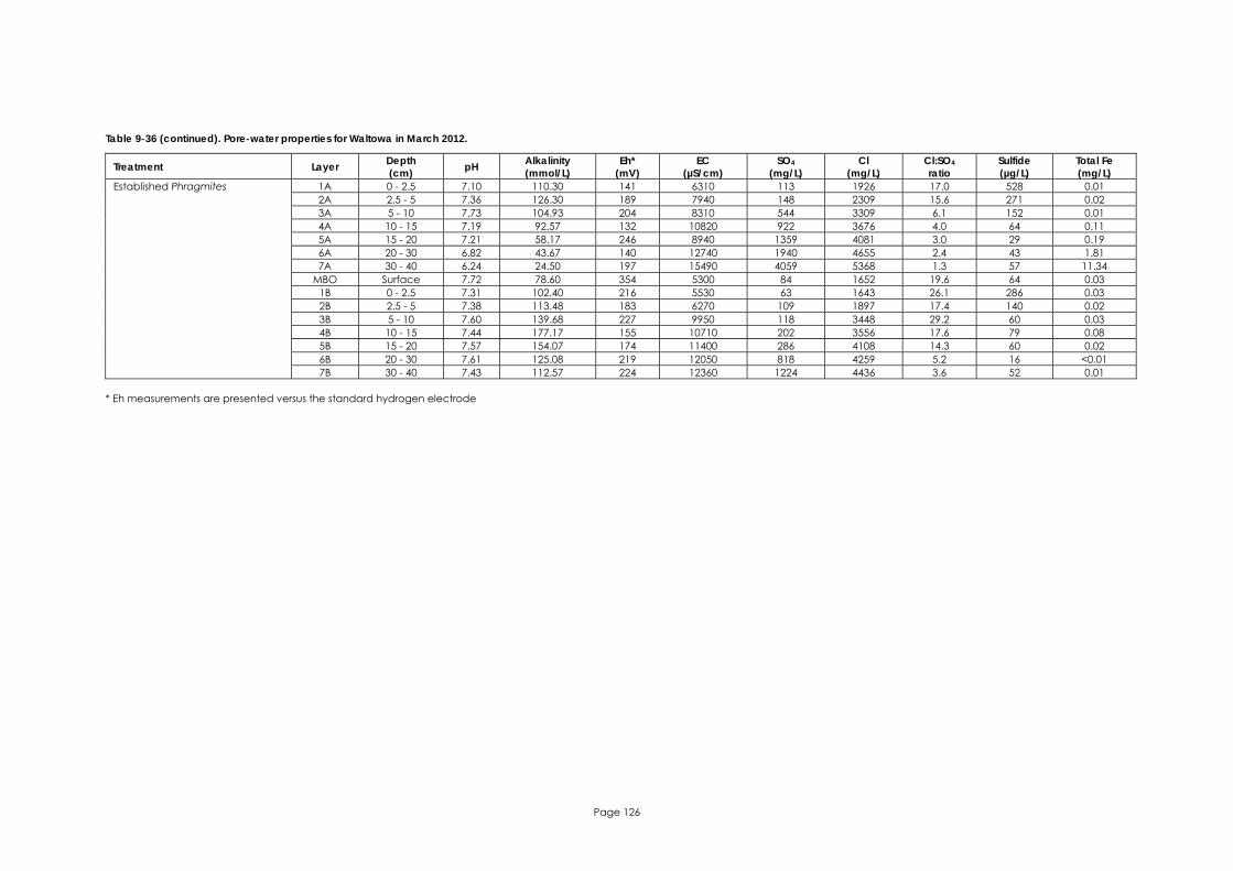
Page 126
Table 9-36 (continued). Pore-water properties for Waltowa in March 2012.
Treatment Layer Depth (cm) pH Alkalinity
(mmol/L) Eh*
(mV) EC
(µS/cm) SO4
(mg/L) Cl
(mg/L) Cl:SO4
ratio Sulfide (µg/L)
Total Fe (mg/L)
1A 0 - 2.5 7.10 110.30 141 6310 113 1926 17.0 528 0.01 2A 2.5 - 5 7.36 126.30 189 7940 148 2309 15.6 271 0.02 3A 5 - 10 7.73 104.93 204 8310 544 3309 6.1 152 0.01 4A 10 - 15 7.19 92.57 132 10820 922 3676 4.0 64 0.11 5A 15 - 20 7.21 58.17 246 8940 1359 4081 3.0 29 0.19 6A 20 - 30 6.82 43.67 140 12740 1940 4655 2.4 43 1.81 7A 30 - 40 6.24 24.50 197 15490 4059 5368 1.3 57 11.34
MBO Surface 7.72 78.60 354 5300 84 1652 19.6 64 0.03 1B 0 - 2.5 7.31 102.40 216 5530 63 1643 26.1 286 0.03 2B 2.5 - 5 7.38 113.48 183 6270 109 1897 17.4 140 0.02 3B 5 - 10 7.60 139.68 227 9950 118 3448 29.2 60 0.03 4B 10 - 15 7.44 177.17 155 10710 202 3556 17.6 79 0.08 5B 15 - 20 7.57 154.07 174 11400 286 4108 14.3 60 0.02 6B 20 - 30 7.61 125.08 219 12050 818 4259 5.2 16 <0.01
Established Phragmites
7B 30 - 40 7.43 112.57 224 12360 1224 4436 3.6 52 0.01 * Eh measurements are presented versus the standard hydrogen electrode

Page 127
Table 9-27. Pore-water soluble cation and nutrient analyses for Waltowa in March 2012.
Treatment Layer Depth (cm) Soluble cations Nutrients
Ca (mg/L)
Mg (mg/L)
Na (mg/L)
K (mg/L)
Nitrate (mg/L N)
Nitrite (mg/L N)
Ammonia (mg/L N)
Orthophosphate (mg/L P)
1A 0 - 2.5 102 201 1106 52 0.14 0.04 6.37 0.01 2A 2.5 - 5 56 120 823 51 0.08 0.02 3.16 0.01 3A 5 - 10 101 198 1181 61 0.14 0.01 6.47 0.01 4A 10 - 15 132 239 1309 55 0.12 0.08 10.30 0.09 5A 15 - 20 198 339 1532 55 0.11 0.03 12.91 0.04 6A 20 - 30 259 429 1882 56 0.09 0.02 15.86 <0.01 7A 30 - 40 274 414 1867 56 0.20 0.11 14.98 0.20 1B 0 - 2.5 64 132 843 51 0.10 0.02 4.80 0.08 2B 2.5 - 5 61 133 841 53 0.29 0.02 4.22 0.02 3B 5 - 10 66 134 1003 51 0.12 0.02 4.17 0.01 4B 10 - 15 110 195 1218 53 0.47 0.04 7.15 0.02 5B 15 - 20 224 345 1634 71 0.64 0.08 12.01 0.08 6B 20 - 30 522 471 1786 95 0.32 0.03 13.28 <0.01
Established Cotula
7B 30 - 40 451 577 2079 77 0.11 0.04 14.01 0.07 1A 0 - 2.5 59 139 892 54 0.23 0.03 3.36 0.08 2A 2.5 - 5 58 133 923 55 0.07 <0.01 1.93 0.02 3A 5 - 10 62 157 1078 56 0.12 0.02 3.74 0.02 4A 10 - 15 83 203 1430 67 <0.01 0.02 6.94 0.02 5A 15 - 20 161 330 1972 72 0.03 0.01 10.10 0.02 6A 20 - 30 287 463 2439 74 0.06 0.02 12.21 0.03 7A 30 - 40 373 603 2947 90 0.11 0.02 18.05 0.02 1B 0 - 2.5 55 131 849 49 0.19 0.03 2.97 0.02 2B 2.5 - 5 61 147 938 53 0.30 0.06 3.07 <0.01 3B 5 - 10 87 172 1209 57 0.02 0.01 3.71 <0.01 4B 10 - 15 121 227 1455 60 <0.01 0.02 5.73 <0.01 5B 15 - 20 200 360 1907 65 0.01 <0.01 7.70 0.01 6B 20 - 30 282 526 2586 69 0.08 0.02 10.73 0.02
Established Juncus
7B 30 - 40 351 600 2792 90 0.12 0.02 20.70 0.03
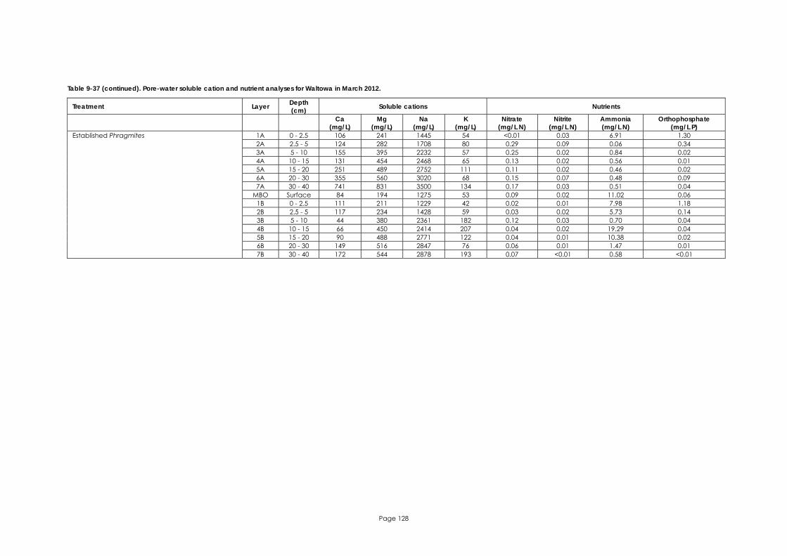
Page 128
Table 9-37 (continued). Pore-water soluble cation and nutrient analyses for Waltowa in March 2012.
Treatment Layer Depth (cm) Soluble cations Nutrients
Ca (mg/L)
Mg (mg/L)
Na (mg/L)
K (mg/L)
Nitrate (mg/L N)
Nitrite (mg/L N)
Ammonia (mg/L N)
Orthophosphate (mg/L P)
1A 0 - 2.5 106 241 1445 54 <0.01 0.03 6.91 1.30 2A 2.5 - 5 124 282 1708 80 0.29 0.09 0.06 0.34 3A 5 - 10 155 395 2232 57 0.25 0.02 0.84 0.02 4A 10 - 15 131 454 2468 65 0.13 0.02 0.56 0.01 5A 15 - 20 251 489 2752 111 0.11 0.02 0.46 0.02 6A 20 - 30 355 560 3020 68 0.15 0.07 0.48 0.09 7A 30 - 40 741 831 3500 134 0.17 0.03 0.51 0.04
MBO Surface 84 194 1275 53 0.09 0.02 11.02 0.06 1B 0 - 2.5 111 211 1229 42 0.02 0.01 7.98 1.18 2B 2.5 - 5 117 234 1428 59 0.03 0.02 5.73 0.14 3B 5 - 10 44 380 2361 182 0.12 0.03 0.70 0.04 4B 10 - 15 66 450 2414 207 0.04 0.02 19.29 0.04 5B 15 - 20 90 488 2771 122 0.04 0.01 10.38 0.02 6B 20 - 30 149 516 2847 76 0.06 0.01 1.47 0.01
Established Phragmites
7B 30 - 40 172 544 2878 193 0.07 <0.01 0.58 <0.01

Page 129
Table 9-28. Pore-water properties for Poltalloch in March 2012.
Treatment Layer Depth (cm) pH Alkalinity
(mmol/L) Eh*
(mV) EC
(µS/cm) SO4
(mg/L) Cl
(mg/L) Cl:SO4
ratio Sulfide (µg/L)
Total Fe (mg/L)
1A 0 - 2.5 7.80 9.67 252 464 92 126 1.4 45 0.01 2A 2.5 - 5 7.69 14.16 256 637 90 149 1.7 10 <0.01 3A 5 - 10 7.11 6.53 277 2130 350 611 1.7 23 <0.01 4A 10 - 15 6.51 3.11 227 2960 673 976 1.5 21 0.35 5A 15 - 20 4.94 2.43 319 5650 1224 1567 1.3 20 5.99 6A 20 - 30 3.87 3.54 416 6110 1838 2453 1.3 16 8.35 7A 30 - 40 4.11 3.49 418 8540 2333 3715 1.6 12 9.06 1B 0 - 2.5 7.62 14.70 330 454 66 111 1.7 16 0.01 2B 2.5 - 5 7.17 13.45 314 485 94 143 1.5 31 0.03 3B 5 - 10 7.77 18.56 320 835 122 254 2.1 14 0.05 4B 10 - 15 7.83 14.71 322 2317 382 718 1.9 52 0.02 5B 15 - 20 7.85 14.47 334 3390 717 1143 1.6 3 <0.01 6B 20 - 30 7.64 17.52 347 7590 1822 2433 1.3 113 0.05
2009 plantings of Bevy rye
7B 30 - 40 7.92 24.12 343 8520 2463 3309 1.3 n.a. 0.03 * Eh measurements are presented versus the standard hydrogen electrode
Table 9-29. Pore-water soluble cation and nutrient analyses for Poltalloch in March 2012.
Treatment Layer Depth (cm) Soluble cations Nutrients
Ca (mg/L)
Mg (mg/L)
Na (mg/L)
K (mg/L)
Nitrate (mg/L N)
Nitrite (mg/L N)
Ammonia (mg/L N)
Orthophosphate (mg/L P)
1A 0 - 2.5 17 12 71 26 0.06 0.01 2.34 0.03 2A 2.5 - 5 29 16 97 15 0.11 0.01 1.90 <0.01 3A 5 - 10 84 57 449 68 0.06 0.03 2.26 0.03 4A 10 - 15 145 111 734 87 0.18 0.01 2.05 0.01 5A 15 - 20 248 190 1154 107 0.32 0.03 2.34 0.01 6A 20 - 30 370 293 1762 75 0.31 0.03 2.23 0.01 7A 30 - 40 431 418 2572 181 0.35 0.02 2.19 0.01 1B 0 - 2.5 18 15 70 13 0.14 0.04 3.78 0.04 2B 2.5 - 5 22 13 96 16 0.10 0.01 2.46 0.03 3B 5 - 10 36 25 202 39 0.12 <0.01 2.51 <0.01 4B 10 - 15 98 73 541 86 0.06 0.01 2.13 <0.01 5B 15 - 20 181 137 881 56 0.02 0.02 2.52 <0.01 6B 20 - 30 406 322 1802 94 0.06 0.02 1.58 <0.01
2009 plantings of Bevy rye
7B 30 - 40 533 448 2358 128 0.07 0.01 1.24 <0.01
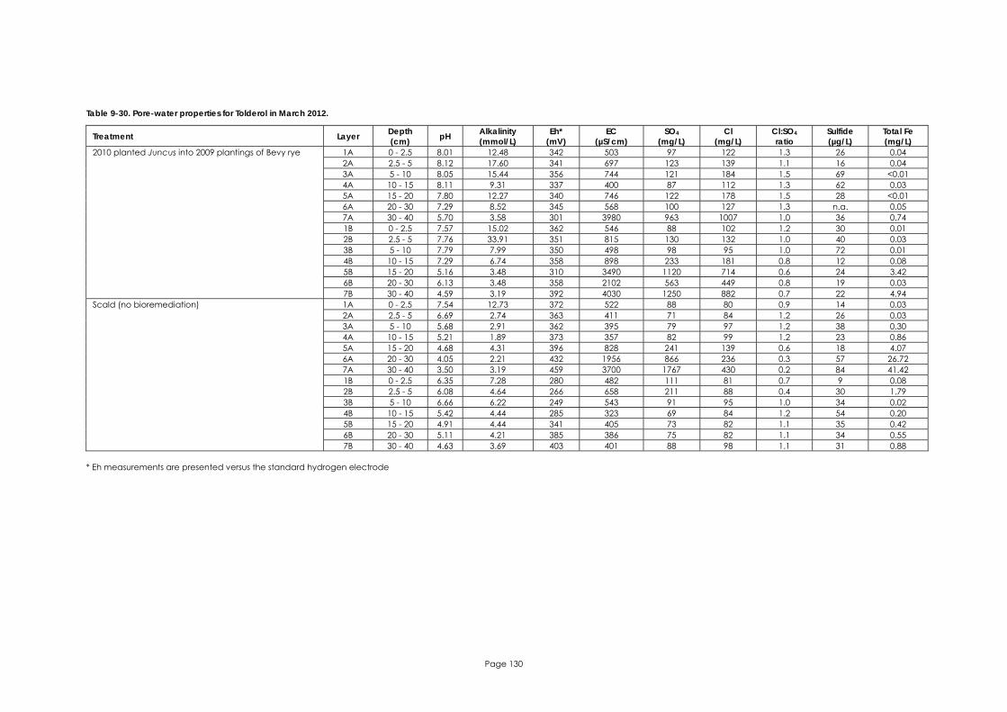
Page 130
Table 9-30. Pore-water properties for Tolderol in March 2012.
Treatment Layer Depth (cm) pH Alkalinity
(mmol/L) Eh*
(mV) EC
(µS/cm) SO4
(mg/L) Cl
(mg/L) Cl:SO4
ratio Sulfide (µg/L)
Total Fe (mg/L)
1A 0 - 2.5 8.01 12.48 342 503 97 122 1.3 26 0.04 2A 2.5 - 5 8.12 17.60 341 697 123 139 1.1 16 0.04 3A 5 - 10 8.05 15.44 356 744 121 184 1.5 69 <0.01 4A 10 - 15 8.11 9.31 337 400 87 112 1.3 62 0.03 5A 15 - 20 7.80 12.27 340 746 122 178 1.5 28 <0.01 6A 20 - 30 7.29 8.52 345 568 100 127 1.3 n.a. 0.05 7A 30 - 40 5.70 3.58 301 3980 963 1007 1.0 36 0.74 1B 0 - 2.5 7.57 15.02 362 546 88 102 1.2 30 0.01 2B 2.5 - 5 7.76 33.91 351 815 130 132 1.0 40 0.03 3B 5 - 10 7.79 7.99 350 498 98 95 1.0 72 0.01 4B 10 - 15 7.29 6.74 358 898 233 181 0.8 12 0.08 5B 15 - 20 5.16 3.48 310 3490 1120 714 0.6 24 3.42 6B 20 - 30 6.13 3.48 358 2102 563 449 0.8 19 0.03
2010 planted Juncus into 2009 plantings of Bevy rye
7B 30 - 40 4.59 3.19 392 4030 1250 882 0.7 22 4.94 1A 0 - 2.5 7.54 12.73 372 522 88 80 0.9 14 0.03 2A 2.5 - 5 6.69 2.74 363 411 71 84 1.2 26 0.03 3A 5 - 10 5.68 2.91 362 395 79 97 1.2 38 0.30 4A 10 - 15 5.21 1.89 373 357 82 99 1.2 23 0.86 5A 15 - 20 4.68 4.31 396 828 241 139 0.6 18 4.07 6A 20 - 30 4.05 2.21 432 1956 866 236 0.3 57 26.72 7A 30 - 40 3.50 3.19 459 3700 1767 430 0.2 84 41.42 1B 0 - 2.5 6.35 7.28 280 482 111 81 0.7 9 0.08 2B 2.5 - 5 6.08 4.64 266 658 211 88 0.4 30 1.79 3B 5 - 10 6.66 6.22 249 543 91 95 1.0 34 0.02 4B 10 - 15 5.42 4.44 285 323 69 84 1.2 54 0.20 5B 15 - 20 4.91 4.44 341 405 73 82 1.1 35 0.42 6B 20 - 30 5.11 4.21 385 386 75 82 1.1 34 0.55
Scald (no bioremediation)
7B 30 - 40 4.63 3.69 403 401 88 98 1.1 31 0.88 * Eh measurements are presented versus the standard hydrogen electrode

Page 131
Table 9-31. Pore-water soluble cation and nutrient analyses for Tolderol in March 2012.
Treatment Layer Depth (cm) Soluble cations Nutrients
Ca (mg/L)
Mg (mg/L)
Na (mg/L)
K (mg/L)
Nitrate (mg/L N)
Nitrite (mg/L N)
Ammonia (mg/L N)
Orthophosphate (mg/L P)
1A 0 - 2.5 23 15 73 42 0.04 <0.01 0.54 <0.01 2A 2.5 - 5 38 21 101 13 0.13 0.01 0.70 <0.01 3A 5 - 10 23 27 121 69 0.22 0.07 0.99 0.06 4A 10 - 15 11 17 79 17 0.10 0.04 0.34 0.02 5A 15 - 20 14 28 119 22 0.06 0.01 0.88 0.04 6A 20 - 30 7 15 98 17 0.07 0.03 0.68 0.09 7A 30 - 40 98 189 820 54 0.07 0.02 2.22 <0.01 1B 0 - 2.5 27 19 78 12 0.15 <0.01 1.32 0.04 2B 2.5 - 5 45 31 105 16 0.09 0.01 1.31 0.02 3B 5 - 10 17 15 79 12 0.11 0.01 0.74 0.01 4B 10 - 15 18 32 154 22 0.28 0.03 2.34 0.01 5B 15 - 20 103 204 646 55 0.23 0.01 4.58 0.02 6B 20 - 30 44 91 394 38 0.11 0.01 2.93 <0.01
2010 planted Juncus into 2009 plantings of Bevy rye
7B 30 - 40 115 216 768 59 0.37 0.03 3.74 0.01 1A 0 - 2.5 20 18 75 11 0.11 0.03 1.22 0.01 2A 2.5 - 5 7 7 67 14 0.06 0.02 0.35 0.02 3A 5 - 10 4 4 66 16 0.14 <0.01 0.70 <0.01 4A 10 - 15 3 5 78 20 0.11 0.01 1.28 0.03 5A 15 - 20 10 17 113 27 0.46 0.01 2.99 0.01 6A 20 - 30 34 57 245 56 <0.01 0.07 5.69 0.01 7A 30 - 40 97 171 471 49 0.63 0.08 8.40 0.01 1B 0 - 2.5 14 14 72 10 0.03 <0.01 0.32 0.01 2B 2.5 - 5 17 20 83 19 0.06 0.02 0.78 0.01 3B 5 - 10 9 8 72 14 0.02 0.02 0.43 <0.01 4B 10 - 15 4 4 65 15 0.10 0.01 0.70 0.01 5B 15 - 20 3 4 72 15 0.07 0.01 1.08 <0.01 6B 20 - 30 2 3 66 15 0.11 0.02 0.95 <0.01
Scald (no bioremediation)
7B 30 - 40 3 4 67 13 0.04 0.10 1.47 <0.01

Page 132
Table 9-32. Pore-water properties for Campbell Park in March 2012.
Treatment Layer Depth (cm) pH Alkalinity
(mmol/L) Eh*
(mV) EC
(µS/cm) SO4
(mg/L) Cl
(mg/L) Cl:SO4
ratio Sulfide (µg/L)
Total Fe (mg/L)
1A 0 - 2.5 7.11 34.08 164 4190 363 1295 3.6 19 0.09 2A 2.5 - 5 6.82 17.83 157 4190 472 1198 2.5 21 0.73 3A 5 - 10 5.83 6.21 230 5640 1334 1460 1.1 90 22.36 4A 10 - 15 4.06 6.07 350 7720 2626 1785 0.7 84 78.43 5A 15 - 20 3.57 4.82 311 8500 2930 1856 0.6 41 76.99 6A 20 - 30 3.48 4.34 441 9000 3240 1983 0.6 66 70.93 7A 30 - 40 3.64 4.96 452 9220 3049 2389 0.8 21 31.84 1B 0 - 2.5 7.29 34.22 171 3950 371 1106 3.0 21 0.05 2B 2.5 - 5 6.46 10.81 179 4480 612 1281 2.1 49 2.90 3B 5 - 10 5.66 5.95 205 5580 1358 1459 1.1 119 18.52 4B 10 - 15 4.03 5.32 288 6630 2333 1480 0.6 85 7.03 5B 15 - 20 3.61 0.32 384 7960 2975 1568 0.5 120 8.88 6B 20 - 30 3.45 3.76 403 9010 3670 1853 0.5 141 8.71
Control (no bioremediation)
7B 30 - 40 4.10 2.67 412 8480 2912 1978 0.7 19 3.48 1A 0 - 2.5 7.19 28.57 261 4150 411 1162 2.8 55 0.17 2A 2.5 - 5 6.46 3.60 178 4470 680 1270 1.9 24 3.16 3A 5 - 10 4.46 3.92 316 6390 1791 1585 0.9 43 24.48 4A 10 - 15 3.82 10.99 383 7890 2895 1791 0.6 104 63.91 5A 15 - 20 3.55 31.98 452 8560 3470 1886 0.5 247 68.21 6A 20 - 30 3.54 31.35 458 9190 3995 2112 0.5 47 46.13 7A 30 - 40 3.80 32.54 452 9790 4394 2382 0.5 27 33.94 1B 0 - 2.5 7.82 46.87 353 4160 395 1161 2.9 74 0.01 2B 2.5 - 5 7.54 21.86 260 4060 434 1155 2.7 116 <0.01 3B 5 - 10 6.99 13.50 215 5830 944 1684 1.8 108 <0.01 4B 10 - 15 4.96 3.80 339 7420 2167 1964 0.9 20 16.20 5B 15 - 20 5.11 3.96 448 8680 3029 2063 0.7 56 55.66 6B 20 - 30 3.79 3.72 438 10900 4604 2676 0.6 47 80.41
2010 seeded with Bevy rye and Puccinellia
7B 30 - 40 3.69 3.23 446 10730 4353 2648 0.6 163 62.74 * Eh measurements are presented versus the standard hydrogen electrode
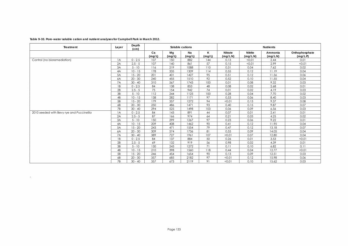
Page 133
Table 9-33. Pore-water soluble cation and nutrient analyses for Campbell Park in March 2012.
Treatment Layer Depth (cm) Soluble cations Nutrients
Ca (mg/L)
Mg (mg/L)
Na (mg/L)
K (mg/L)
Nitrate (mg/L N)
Nitrite (mg/L N)
Ammonia (mg/L N)
Orthophosphate (mg/L P)
1A 0 - 2.5 107 150 882 144 0.13 <0.01 2.44 0.01 2A 2.5 - 5 107 140 861 57 0.15 <0.01 2.99 <0.01 3A 5 - 10 116 219 1088 110 0.31 0.04 7.62 0.02 4A 10 - 15 178 335 1309 114 0.55 0.12 11.19 0.04 5A 15 - 20 201 401 1427 95 0.51 0.12 11.56 0.06 6A 20 - 30 240 455 1510 92 0.52 0.10 11.55 0.04 7A 30 - 40 310 567 1743 100 0.01 0.08 9.32 0.03 1B 0 - 2.5 84 138 853 48 0.08 0.02 2.68 0.01 2B 2.5 - 5 75 154 942 74 0.01 0.02 4.19 0.03 3B 5 - 10 112 244 1125 100 0.28 0.04 7.70 0.02 4B 10 - 15 138 282 1171 97 0.53 0.06 8.40 0.03 5B 15 - 20 179 357 1272 94 <0.01 0.13 9.37 0.08 6B 20 - 30 250 486 1471 93 0.40 0.15 9.87 0.07
Control (no bioremediation)
7B 30 - 40 294 525 1498 103 0.06 0.09 6.56 0.03 1A 0 - 2.5 84 143 891 44 0.07 0.01 2.41 0.01 2A 2.5 - 5 87 166 974 64 0.21 0.03 4.25 0.02 3A 5 - 10 150 299 1267 97 0.23 0.06 9.22 0.01 4A 10 - 15 209 408 1462 90 0.41 0.12 11.95 0.04 5A 15 - 20 243 471 1554 79 0.47 0.12 13.18 0.07 6A 20 - 30 309 574 1736 81 0.55 0.09 14.05 0.04 7A 30 - 40 389 727 1961 107 <0.01 0.07 12.80 0.04 1B 0 - 2.5 84 137 884 50 0.26 0.01 3.53 <0.01 2B 2.5 - 5 69 132 919 56 0.98 0.02 4.39 0.01 3B 5 - 10 130 243 1272 71 0.11 0.10 6.82 0.11 4B 10 - 15 210 398 1560 118 0.44 0.04 12.77 <0.01 5B 15 - 20 246 454 1654 90 0.13 0.09 12.51 0.03 6B 20 - 30 357 685 2182 97 <0.01 0.12 15.98 0.06
2010 seeded with Bevy rye and Puccinellia
7B 30 - 40 357 673 2119 91 <0.01 0.10 15.62 0.03
.

Page 134
APPENDIX 5. Pore-water plots

Page 135
0
5
10
15
20
25
30
35
40
0 100 200 300 400 500
Depth (cm)
Eh (mV)
Phragmites
Cotula
Juncus
Figure 9-1. Pore-water Eh characteristics at the Waltowa study area (March 2012).
0
5
10
15
20
25
30
35
40
0 100 200 300 400 500
Depth (cm)
Eh (mV)
Bioremediated
Figure 9-2. Pore-water Eh characteristics at the Poltalloch Bevy rye site (March 2012).
0
5
10
15
20
25
30
35
40
0 100 200 300 400 500
Depth (cm)
Eh (mV)
Scald
Bioremediated

Page 136
Figure 9-3. Pore-water Eh characteristics at the Tolderol study area (March 2012).
0
5
10
15
20
25
30
35
40
0 100 200 300 400 500
Depth (cm)
Eh (mV)
Scald
Bioremediated
Figure 9-4. Pore-water Eh characteristics at the Campbell Park study area (March 2012).
0
5
10
15
20
25
30
35
40
2 4 6 8 10
Depth (cm)
pH
Phragmites
Cotula
Juncus
Phragmites MBO
Figure 9-5. Pore-water pH characteristics at the Waltowa study area (March 2012).
0
5
10
15
20
25
30
35
40
2 4 6 8 10
Depth (cm)
pH
Bioremediated
Figure 9-6. Pore-water pH characteristics at the Poltalloch Bevy rye site (March 2012).

Page 137
0
5
10
15
20
25
30
35
40
2 4 6 8 10
Depth (cm)
pH
Scald
Bioremediated
Figure 9-7. Pore-water pH characteristics at the Tolderol study area (March 2012).
0
5
10
15
20
25
30
35
40
2 4 6 8 10
Depth (cm)
pH
Scald
Bioremediated
Figure 9-8. Pore-water pH characteristics at the Campbell Park study area (March 2012).
0
5
10
15
20
25
30
35
40
0 5000 10000 15000 20000
Depth (cm)
EC (µS/cm)
Phragmites
Cotula
Juncus
Phragmites MBO
Figure 9-9. Pore-water EC characteristics at the Waltowa study area (March 2012).

Page 138
0
5
10
15
20
25
30
35
40
0 5000 10000 15000 20000
Depth (cm)
EC (µS/cm)
Bioremediated
Figure 9-10. Pore-water EC characteristics at the Poltalloch Bevy rye site (March 2012).
0
5
10
15
20
25
30
35
40
0 5000 10000 15000 20000
Depth (cm)
EC (µS/cm)
Scald
Bioremediated
Figure 9-11. Pore-water EC characteristics at the Tolderol study area (March 2012).
0
5
10
15
20
25
30
35
40
0 5000 10000 15000 20000
Depth (cm)
EC (µS/cm)
Scald
Bioremediated
Figure 9-12. Pore-water EC characteristics at the Campbell Park study area (March 2012).

Page 139
0
5
10
15
20
25
30
35
40
0 50 100 150 200
Depth (cm)
Alkalinity (mmol/L)
Phragmites
Cotula
Juncus
Phragmites MBO
Figure 9-13. Pore-water alkalinity characteristics at the Waltowa study area (March 2012).
0
5
10
15
20
25
30
35
40
0 20 40 60
Depth (cm)
Alkalinity (mmol/L)
Bioremediated
Figure 9-14. Pore-water alkalinity characteristics at the Poltalloch Bevy rye site (March 2012).
0
5
10
15
20
25
30
35
40
0 20 40 60
Depth (cm)
Alkalinity (mmol/L)
Scald
Bioremediated
Figure 9-15. Pore-water alkalinity characteristics at the Tolderol study area (March 2012).

Page 140
0
5
10
15
20
25
30
35
40
0 20 40 60
Depth (cm)
Alkalinity (mmol/L)
Scald
Bioremediated
Figure 9-16. Pore-water alkalinity characteristics at the Campbell Park study area (March 2012).
0
5
10
15
20
25
30
35
40
0 200 400 600
Depth (cm)
Sulfide (µg/L)
Phragmites
Cotula
Juncus
Phragmites MBO
Figure 9-17. Pore-water dissolved sulfide characteristics at the Waltowa study area (March 2012).
0
5
10
15
20
25
30
35
40
0 100 200 300
Depth (cm)
Sulfide (µg/L)
Bioremediated
Figure 9-18. Pore-water dissolved sulfide characteristics at the Poltalloch Bevy rye site (March 2012).

Page 141
0
5
10
15
20
25
30
35
40
0 100 200 300
Depth (cm)
Sulfide (µg/L)
Scald
Bioremediated
Figure 9-19. Pore-water dissolved sulfide characteristics at the Tolderol study area (March 2012).
0
5
10
15
20
25
30
35
40
0 100 200 300
Depth (cm)
Sulfide (µg/L)
Scald
Bioremediated
Figure 9-20. Pore-water dissolved sulfide characteristics at the Campbell Park study area (March 2012).
0
5
10
15
20
25
30
35
40
0 5 10 15
Depth (cm)
Total Fe (mg/L)
Phragmites
Cotula
Juncus
Phragmites MBO
Figure 9-21. Pore-water total dissolved iron (Fe3+ + Fe2+) characteristics at the Waltowa study area (March 2012).

Page 142
0
5
10
15
20
25
30
35
40
0 5 10 15
Depth (cm)
Total Fe (mg/L)
Bioremediated
Figure 9-22. Pore-water total dissolved iron (Fe3+ + Fe2+) characteristics at the Poltalloch Bevy rye site (March 2012).
0
5
10
15
20
25
30
35
40
0 20 40 60
Depth (cm)
Total Fe (mg/L)
Scald
Bioremediated
Figure 9-23. Pore-water total dissolved iron (Fe3+ + Fe2+) characteristics at the Tolderol study area (March 2012).
0
5
10
15
20
25
30
35
40
0 50 100 150
Depth (cm)
Total Fe (mg/L)
Scald
Bioremediated
Figure 9-24. Pore-water total dissolved iron (Fe3+ + Fe2+) characteristics at the Campbell Park study area (March 2012).

Page 143
0
5
10
15
20
25
30
35
40
0 2000 4000 6000
Depth (cm)
Chloride (mg/L)
Phragmites
Cotula
Juncus
Phragmites MBO
Figure 9-25. Pore-water soluble chloride characteristics at the Waltowa study area (March 2012).
0
5
10
15
20
25
30
35
40
0 1000 2000 3000 4000
Depth (cm)
Chloride (mg/L)
Bioremediated
Figure 9-26. Pore-water soluble chloride characteristics at the Poltalloch Bevy rye site (March 2012).
0
5
10
15
20
25
30
35
40
0 500 1000 1500 2000
Depth (cm)
Chloride (mg/L)
Scald
Bioremediated
Figure 9-27. Pore-water soluble chloride characteristics at the Tolderol study area (March 2012).
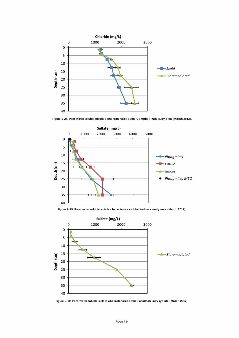
Page 144
0
5
10
15
20
25
30
35
40
0 1000 2000 3000
Depth (cm)
Chloride (mg/L)
Scald
Bioremediated
Figure 9-28. Pore-water soluble chloride characteristics at the Campbell Park study area (March 2012).
0
5
10
15
20
25
30
35
40
0 1000 2000 3000 4000 5000
Depth (cm)
Sulfate (mg/L)
Phragmites
Cotula
Juncus
Phragmites MBO
Figure 9-29. Pore-water soluble sulfate characteristics at the Waltowa study area (March 2012).
0
5
10
15
20
25
30
35
40
0 1000 2000 3000
Depth (cm)
Sulfate (mg/L)
Bioremediated
Figure 9-30. Pore-water soluble sulfate characteristics at the Poltalloch Bevy rye site (March 2012).

Page 145
0
5
10
15
20
25
30
35
40
0 500 1000 1500 2000
Depth (cm)
Sulfate (mg/L)
Scald
Bioremediated
Figure 9-31. Pore-water soluble sulfate characteristics at the Tolderol study area (March 2012).
0
5
10
15
20
25
30
35
40
0 1000 2000 3000 4000 5000
Depth (cm)
Sulfate (mg/L)
Scald
Bioremediated
Figure 9-32. Pore-water soluble sulfate characteristics at the Campbell Park study area (March 2012).
0
5
10
15
20
25
30
35
40
0 200 400 600 800
Depth (cm)
Ca (mg/L)
Phragmites
Cotula
Juncus
Phragmites MBO
Figure 9-33. Pore-water soluble calcium characteristics at the Waltowa study area (March 2012).
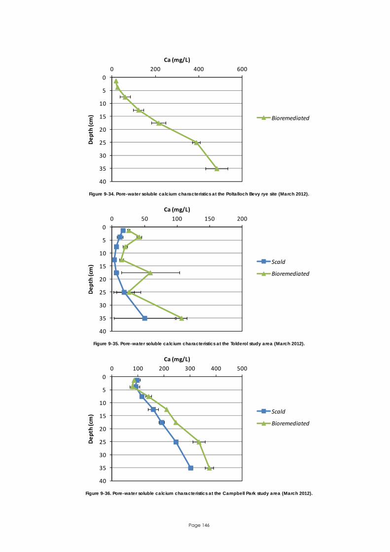
Page 146
0
5
10
15
20
25
30
35
40
0 200 400 600
Depth (cm)
Ca (mg/L)
Bioremediated
Figure 9-34. Pore-water soluble calcium characteristics at the Poltalloch Bevy rye site (March 2012).
0
5
10
15
20
25
30
35
40
0 50 100 150 200
Depth (cm)
Ca (mg/L)
Scald
Bioremediated
Figure 9-35. Pore-water soluble calcium characteristics at the Tolderol study area (March 2012).
0
5
10
15
20
25
30
35
40
0 100 200 300 400 500
Depth (cm)
Ca (mg/L)
Scald
Bioremediated
Figure 9-36. Pore-water soluble calcium characteristics at the Campbell Park study area (March 2012).
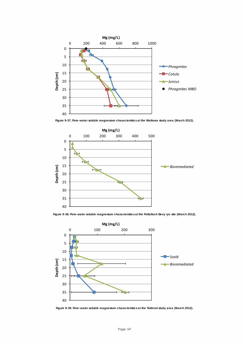
Page 147
0
5
10
15
20
25
30
35
40
0 200 400 600 800 1000
Depth (cm)
Mg (mg/L)
Phragmites
Cotula
Juncus
Phragmites MBO
Figure 9-37. Pore-water soluble magnesium characteristics at the Waltowa study area (March 2012).
0
5
10
15
20
25
30
35
40
0 100 200 300 400 500
Depth (cm)
Mg (mg/L)
Bioremediated
Figure 9-38. Pore-water soluble magnesium characteristics at the Poltalloch Bevy rye site (March 2012).
0
5
10
15
20
25
30
35
40
0 100 200 300
Depth (cm)
Mg (mg/L)
Scald
Bioremediated
Figure 9-39. Pore-water soluble magnesium characteristics at the Tolderol study area (March 2012).

Page 148
0
5
10
15
20
25
30
35
40
0 200 400 600 800
Depth (cm)
Mg (mg/L)
Scald
Bioremediated
Figure 9-40. Pore-water soluble magnesium characteristics at the Campbell Park study area (March 2012).
0
5
10
15
20
25
30
35
40
0 1000 2000 3000 4000
Depth (cm)
Na (mg/L)
Phragmites
Cotula
Juncus
Phragmites MBO
Figure 9-41. Pore-water soluble sodium characteristics at the Waltowa study area (March 2012).
0
5
10
15
20
25
30
35
40
0 1000 2000 3000
Depth (cm)
Na (mg/L)
Bioremediated
Figure 9-42. Pore-water soluble sodium characteristics at the Poltalloch Bevy rye site (March 2012).

Page 149
0
5
10
15
20
25
30
35
40
0 200 400 600 800 1000
Depth (cm)
Na (mg/L)
Scald
Bioremediated
Figure 9-43. Pore-water soluble sodium characteristics at the Tolderol study area (March 2012).
0
5
10
15
20
25
30
35
40
0 500 1000 1500 2000 2500
Depth (cm)
Na (mg/L)
Scald
Bioremediated
Figure 9-44. Pore-water soluble sodium characteristics at the Campbell Park study area (March 2012).
0
5
10
15
20
25
30
35
40
0 100 200 300
Depth (cm)
K (mg/L)
Phragmites
Cotula
Juncus
Phragmites MBO
Figure 9-45. Pore-water soluble potassium characteristics at the Waltowa study area (March 2012).

Page 150
0
5
10
15
20
25
30
35
40
0 50 100 150 200
Depth (cm)
K (mg/L)
Bioremediated
Figure 9-46. Pore-water soluble potassium characteristics at the Poltalloch Bevy rye site (March 2012).
0
5
10
15
20
25
30
35
40
0 50 100 150 200
Depth (cm)
K (mg/L)
Scald
Bioremediated
Figure 9-47. Pore-water soluble potassium characteristics at the Tolderol study area (March 2012).
0
5
10
15
20
25
30
35
40
0 50 100 150 200
Depth (cm)
K (mg/L)
Scald
Bioremediated
Figure 9-48. Pore-water soluble potassium characteristics at the Campbell Park study area (March 2012).

Page 151
0
5
10
15
20
25
30
35
40
0.00 0.50 1.00 1.50
Depth (cm)
Orthophosphate (mg/L P)
Phragmites
Cotula
Juncus
Phragmites MBO
Figure 9-49. Pore-water orthophosphate characteristics at the Waltowa study area (March 2012).
0
5
10
15
20
25
30
35
40
0.00 0.02 0.04 0.06 0.08 0.10
Depth (cm)
Orthophosphate (mg/L P)
Bioremediated
Figure 9-50. Pore-water orthophosphate characteristics at the Poltalloch Bevy rye site (March 2012).
0
5
10
15
20
25
30
35
40
0.00 0.05 0.10 0.15
Depth (cm)
Orthophosphate (mg/L P)
Scald
Bioremediated
Figure 9-51. Pore-water orthophosphate characteristics at the Tolderol study area (March 2012).

Page 152
0
5
10
15
20
25
30
35
40
0.00 0.05 0.10 0.15
Depth (cm)
Orthophosphate (mg/L P)
Scald
Bioremediated
Figure 9-52. Pore-water orthophosphate characteristics at the Campbell Park study area (March 2012).
0
5
10
15
20
25
30
35
40
0.0 0.2 0.4 0.6 0.8
Depth (cm)
Nitrate (mg/L N)
Phragmites
Cotula
Juncus
Phragmites MBO
Figure 9-53. Pore-water nitrate characteristics at the Waltowa study area (March 2012).
0
5
10
15
20
25
30
35
40
0.0 0.1 0.2 0.3 0.4 0.5
Depth (cm)
Nitrate (mg/L N)
Bioremediated
Figure 9-54. Pore-water nitrate characteristics at the Poltalloch Bevy rye site (March 2012).

Page 153
0
5
10
15
20
25
30
35
40
0.0 0.2 0.4 0.6 0.8
Depth (cm)
Nitrate (mg/L N)
Scald
Bioremediated
Figure 9-55. Pore-water nitrate characteristics at the Tolderol study area (March 2012).
Figure 9-56. Pore-water nitrate characteristics at the Campbell Park study area (March 2012).
0
5
10
15
20
25
30
35
40
0.00 0.05 0.10 0.15
Depth (cm)
Nitrate (mg/L N)
Phragmites
Cotula
Juncus
Phragmites MBO
Figure 9-57. Pore-water nitrite characteristics at the Waltowa study area (March 2012).

Page 154
0
5
10
15
20
25
30
35
40
0.00 0.02 0.04 0.06 0.08 0.10
Depth (cm)
Nitrite (mg/L N)
Bioremediated
Figure 9-58. Pore-water nitrite characteristics at the Poltalloch Bevy rye site (March 2012).
0
5
10
15
20
25
30
35
40
0.00 0.05 0.10 0.15
Depth (cm)
Nitrite (mg/L N)
Scald
Bioremediated
Figure 9-59. Pore-water nitrite characteristics at the Tolderol study area (March 2012).
0
5
10
15
20
25
30
35
40
0.00 0.05 0.10 0.15 0.20
Depth (cm)
Nitrite (mg/L N)
Scald
Bioremediated
Figure 9-60. Pore-water nitrite characteristics at the Campbell Park study area (March 2012).

Page 155
0
5
10
15
20
25
30
35
40
0 5 10 15 20 25
Depth (cm)
Ammonia (mg/L N)
Phragmites
Cotula
Juncus
Phragmites MBO
Figure 9-61. Pore-water ammonia characteristics at the Waltowa study area (March 2012).
0
5
10
15
20
25
30
35
40
0 1 2 3 4 5
Depth (cm)
Ammonia (mg/L N)
Bioremediated
Figure 9-62. Pore-water ammonia characteristics at the Poltalloch Bevy rye site (March 2012).
0
5
10
15
20
25
30
35
40
0 2 4 6 8 10
Depth (cm)
Ammonia (mg/L N)
Scald
Bioremediated
Figure 9-63. Pore-water ammonia characteristics at the Tolderol study area (March 2012).
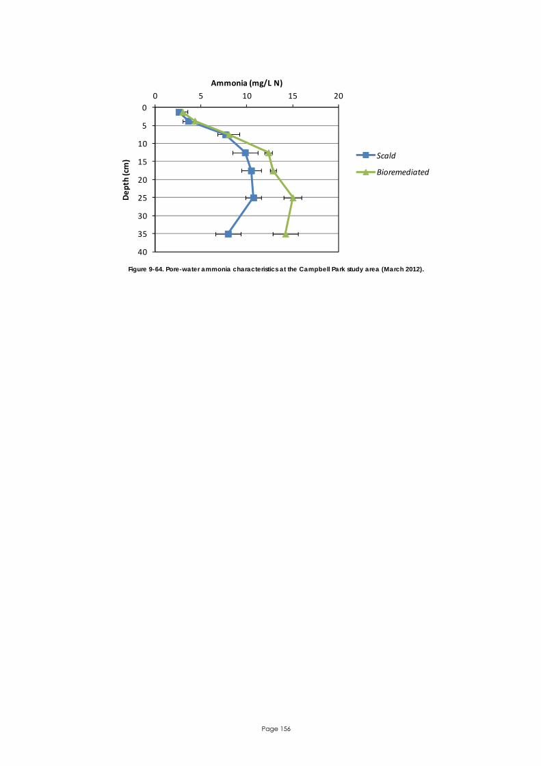
Page 156
0
5
10
15
20
25
30
35
40
0 5 10 15 20
Depth (cm)
Ammonia (mg/L N)
Scald
Bioremediated
Figure 9-64. Pore-water ammonia characteristics at the Campbell Park study area (March 2012).

Page 157
APPENDIX 6. HCl extractable metal plots
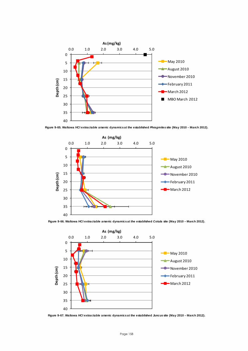
Page 158
0
5
10
15
20
25
30
35
40
0.0 1.0 2.0 3.0 4.0 5.0
Depth (cm)
As (mg/kg)
May 2010
August 2010
November 2010
February 2011
March 2012
MBO March 2012
Figure 9-65. Waltowa HCl extractable arsenic dynamics at the established Phragmites site (May 2010 – March 2012).
0
5
10
15
20
25
30
35
40
0.0 1.0 2.0 3.0 4.0 5.0
Depth (cm)
As (mg/kg)
May 2010
August 2010
November 2010
February 2011
March 2012
Figure 9-66. Waltowa HCl extractable arsenic dynamics at the established Cotula site (May 2010 – March 2012).
0
5
10
15
20
25
30
35
40
0.0 1.0 2.0 3.0 4.0 5.0
Depth (cm)
As (mg/kg)
May 2010
August 2010
November 2010
February 2011
March 2012
Figure 9-67. Waltowa HCl extractable arsenic dynamics at the established Juncus site (May 2010 – March 2012).
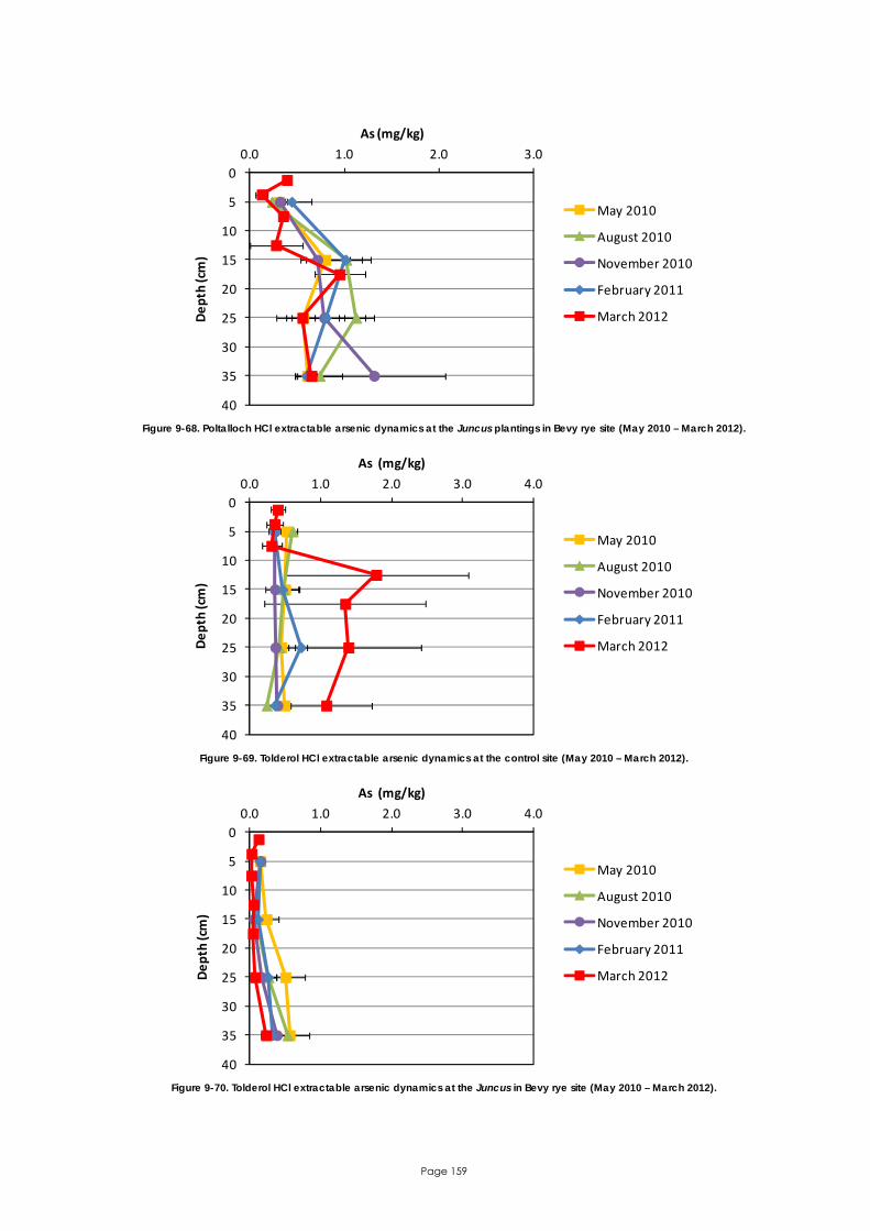
Page 159
0
5
10
15
20
25
30
35
40
0.0 1.0 2.0 3.0
Depth (cm)
As (mg/kg)
May 2010
August 2010
November 2010
February 2011
March 2012
Figure 9-68. Poltalloch HCl extractable arsenic dynamics at the Juncus plantings in Bevy rye site (May 2010 – March 2012).
0
5
10
15
20
25
30
35
40
0.0 1.0 2.0 3.0 4.0
Depth (cm)
As (mg/kg)
May 2010
August 2010
November 2010
February 2011
March 2012
Figure 9-69. Tolderol HCl extractable arsenic dynamics at the control site (May 2010 – March 2012).
0
5
10
15
20
25
30
35
40
0.0 1.0 2.0 3.0 4.0
Depth (cm)
As (mg/kg)
May 2010
August 2010
November 2010
February 2011
March 2012
Figure 9-70. Tolderol HCl extractable arsenic dynamics at the Juncus in Bevy rye site (May 2010 – March 2012).

Page 160
0
5
10
15
20
25
30
35
40
0.0 0.5 1.0 1.5 2.0
Depth (cm)
As (mg/kg)
August 2010
November 2010
February 2011
March 2012
Figure 9-71. Campbell Park HCl extractable arsenic dynamics at the control site (August 2010 – March 2012).
0
5
10
15
20
25
30
35
40
0.0 0.5 1.0 1.5 2.0
Depth (cm)
As (mg/kg)
August 2010
November 2010
February 2011
March 2012
Figure 9-72. Campbell Park HCl extractable arsenic dynamics at the Bevy rye/Puccinellia site (August 2010 – March 2012).
0
5
10
15
20
25
30
35
40
0 5 10 15 20
Depth (cm)
Cu (mg/kg)
May 2010
August 2010
November 2010
February 2011
March 2012
MBO March 2012
Figure 9-73. Waltowa HCl extractable copper dynamics at the established Phragmites site (May 2010 – March 2012).

Page 161
0
5
10
15
20
25
30
35
40
0 5 10 15 20
Depth (cm)
Cu (mg/kg)
May 2010
August 2010
November 2010
February 2011
March 2012
Figure 9-74. Waltowa HCl extractable copper dynamics at the established Cotula site (May 2010 – March 2012).
0
5
10
15
20
25
30
35
40
0.0 1.0 2.0 3.0 4.0 5.0
Depth (cm)
Cu (mg/kg)
May 2010
August 2010
November 2010
February 2011
March 2012
Figure 9-75. Waltowa HCl extractable copper dynamics at the established Juncus site (May 2010 – March 2012).
0
5
10
15
20
25
30
35
40
0.0 1.0 2.0 3.0
Depth (cm)
Cu (mg/kg)
May 2010
August 2010
November 2010
February 2011
March 2012
Figure 9-76. Poltalloch HCl extractable copper dynamics at the Juncus plantings in Bevy rye site (May 2010 – March 2012).

Page 162
0
5
10
15
20
25
30
35
40
0 2 4 6 8
Depth (cm)
Cu (mg/kg)
May 2010
August 2010
November 2010
February 2011
March 2012
Figure 9-77. Tolderol HCl extractable copper dynamics at the control site (May 2010 – March 2012).
0
5
10
15
20
25
30
35
40
0 1 2 3 4
Depth (cm)
Cu (mg/kg)
May 2010
August 2010
November 2010
February 2011
March 2012
Figure 9-78. Tolderol HCl extractable copper dynamics at the Juncus in Bevy rye site (May 2010 – March 2012).
0
5
10
15
20
25
30
35
40
0 2 4 6 8 10
Depth (cm)
Cu (mg/kg)
August 2010
November 2010
February 2011
March 2012
Figure 9-79. Campbell Park HCl extractable copper dynamics at the control site (August 2010 – March 2012).

Page 163
0
5
10
15
20
25
30
35
40
0 2 4 6 8 10
Depth (cm)
Cu (mg/kg)
August 2010
November 2010
February 2011
March 2012
Figure 9-80. Campbell Park HCl extractable copper dynamics at the Bevy rye/Puccinellia site (August 2010 – March 2012).
0
5
10
15
20
25
30
35
40
0 1000 2000 3000 4000 5000
Depth (cm)
Fe (mg/kg)
May 2010
August 2010
November 2010
February 2011
March 2012
MBO March 2012
Figure 9-81. Waltowa HCl extractable iron dynamics at the established Phragmites site (May 2010 – March 2012).
0
5
10
15
20
25
30
35
40
0 1000 2000 3000 4000 5000
Depth (cm)
Fe (mg/kg)
May 2010
August 2010
November 2010
February 2011
March 2012
Figure 9-82. Waltowa HCl extractable iron dynamics at the established Cotula site (May 2010 – March 2012).
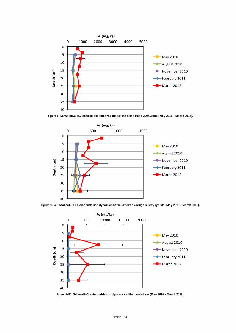
Page 164
0
5
10
15
20
25
30
35
40
0 1000 2000 3000 4000 5000
Depth (cm)
Fe (mg/kg)
May 2010
August 2010
November 2010
February 2011
March 2012
Figure 9-83. Waltowa HCl extractable iron dynamics at the established Juncus site (May 2010 – March 2012).
0
5
10
15
20
25
30
35
40
0 500 1000 1500
Depth (cm)
Fe (mg/kg)
May 2010
August 2010
November 2010
February 2011
March 2012
Figure 9-84. Poltalloch HCl extractable iron dynamics at the Juncus plantings in Bevy rye site (May 2010 – March 2012).
0
5
10
15
20
25
30
35
40
0 5000 10000 15000 20000
Depth (cm)
Fe (mg/kg)
May 2010
August 2010
November 2010
February 2011
March 2012
Figure 9-85. Tolderol HCl extractable iron dynamics at the control site (May 2010 – March 2012).

Page 165
0
5
10
15
20
25
30
35
40
0 500 1000 1500 2000 2500
Depth (cm)
Fe (mg/kg)
May 2010
August 2010
November 2010
February 2011
March 2012
Figure 9-86. Tolderol HCl extractable iron dynamics at the Juncus in Bevy rye site (May 2010 – March 2012).
0
5
10
15
20
25
30
35
40
0 500 1000 1500 2000
Depth (cm)
Fe (mg/kg)
August 2010
November 2010
February 2011
March 2012
Figure 9-87. Campbell Park HCl extractable iron dynamics at the control site (August 2010 – March 2012).
0
5
10
15
20
25
30
35
40
0 500 1000 1500 2000
Depth (cm)
Fe (mg/kg)
August 2010
November 2010
February 2011
March 2012
Figure 9-88. Campbell Park HCl extractable iron dynamics at the Bevy rye/Puccinellia site (August 2010 – March 2012).

Page 166
0
5
10
15
20
25
30
35
40
0 50 100 150 200 250
Depth (cm)
Mn (mg/kg)
May 2010
August 2010
November 2010
February 2011
March 2012
MBO March 2012
Figure 9-89. Waltowa HCl extractable manganese dynamics at the established Phragmites site (May 2010 – March 2012).
0
5
10
15
20
25
30
35
40
0 20 40 60 80 100
Depth (cm)
Mn (mg/kg)
May 2010
August 2010
November 2010
February 2011
March 2012
Figure 9-90. Waltowa HCl extractable manganese dynamics at the established Cotula site (May 2010 – March 2012).
0
5
10
15
20
25
30
35
40
0 20 40 60 80 100
Depth (cm)
Mn (mg/kg)
May 2010
August 2010
November 2010
February 2011
March 2012
Figure 9-91. Waltowa HCl extractable manganese dynamics at the established Juncus site (May 2010 – March 2012).

Page 167
0
5
10
15
20
25
30
35
40
0 20 40 60
Depth (cm)
Mn (mg/kg)
May 2010
August 2010
November 2010
February 2011
March 2012
Figure 9-92. Poltalloch HCl extractable manganese dynamics at the Juncus plantings in Bevy rye site
(May 2010 – March 2012).
0
5
10
15
20
25
30
35
40
0 50 100 150 200
Depth (cm)
Mn (mg/kg)
May 2010
August 2010
November 2010
February 2011
March 2012
Figure 9-93. Tolderol HCl extractable manganese dynamics at the control site (May 2010 – March 2012).
0
5
10
15
20
25
30
35
40
0 10 20 30 40
Depth (cm)
Mn (mg/kg)
May 2010
August 2010
November 2010
February 2011
March 2012
Figure 9-94. Tolderol HCl extractable manganese dynamics at the Juncus in Bevy rye site (May 2010 – March 2012).

Page 168
0
5
10
15
20
25
30
35
40
0 20 40 60 80
Depth (cm)
Mn (mg/kg)
August 2010
November 2010
February 2011
March 2012
Figure 9-95. Campbell Park HCl extractable manganese dynamics at the control site (August 2010 – March 2012).
0
5
10
15
20
25
30
35
40
0 20 40 60 80 100
Depth (cm)
Mn (mg/kg)
August 2010
November 2010
February 2011
March 2012
Figure 9-96. Campbell Park HCl extractable manganese dynamics at the Bevy rye/Puccinellia site (August 2010 – March
2012).
0
5
10
15
20
25
30
35
40
0 2 4 6 8 10
Depth (cm)
Ni (mg/kg)
May 2010
August 2010
November 2010
February 2011
March 2012
MBO March 2012
Figure 9-97. Waltowa HCl extractable nickel dynamics at the established Phragmites site (May 2010 – March 2012).

Page 169
0
5
10
15
20
25
30
35
40
0.0 2.0 4.0 6.0
Depth (cm)
Ni (mg/kg)
May 2010
August 2010
November 2010
February 2011
March 2012
Figure 9-98. Waltowa HCl extractable nickel dynamics at the established Cotula site (May 2010 – March 2012).
0
5
10
15
20
25
30
35
40
0.0 2.0 4.0 6.0
Depth (cm)
Ni (mg/kg)
May 2010
August 2010
November 2010
February 2011
March 2012
Figure 9-99. Waltowa HCl extractable nickel dynamics at the established Juncus site (May 2010 – March 2012).
0
5
10
15
20
25
30
35
40
0.0 0.5 1.0 1.5
Depth (cm)
Ni (mg/kg)
May 2010
August 2010
November 2010
February 2011
March 2012
Figure 9-100. Poltalloch HCl extractable nickel dynamics at the Juncus plantings in Bevy rye site (May 2010 – March 2012).
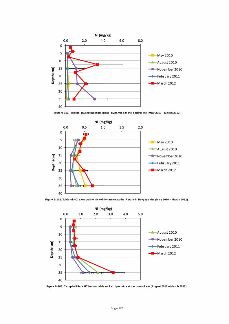
Page 170
0
5
10
15
20
25
30
35
40
0.0 2.0 4.0 6.0 8.0
Depth (cm)
Ni (mg/kg)
May 2010
August 2010
November 2010
February 2011
March 2012
Figure 9-101. Tolderol HCl extractable nickel dynamics at the control site (May 2010 – March 2012).
0
5
10
15
20
25
30
35
40
0.0 0.5 1.0 1.5 2.0
Depth (cm)
Ni (mg/kg)
May 2010
August 2010
November 2010
February 2011
March 2012
Figure 9-102. Tolderol HCl extractable nickel dynamics at the Juncus in Bevy rye site (May 2010 – March 2012).
0
5
10
15
20
25
30
35
40
0.0 1.0 2.0 3.0 4.0 5.0
Depth (cm)
Ni (mg/kg)
August 2010
November 2010
February 2011
March 2012
Figure 9-103. Campbell Park HCl extractable nickel dynamics at the control site (August 2010 – March 2012).

Page 171
0
5
10
15
20
25
30
35
40
0.0 1.0 2.0 3.0 4.0 5.0
Depth (cm)
Ni (mg/kg)
August 2010
November 2010
February 2011
March 2012
Figure 9-104. Campbell Park HCl extractable nickel dynamics at the Bevy rye/Puccinellia site (August 2010 – March 2012).
0
5
10
15
20
25
30
35
40
0 5 10 15 20 25
Depth (cm)
Zn (mg/kg)
May 2010
August 2010
November 2010
February 2011
March 2012
MBO March 2012
Figure 9-105. Waltowa HCl extractable zinc dynamics at the established Phragmites site (May 2010 – March 2012).
0
5
10
15
20
25
30
35
40
0 2 4 6 8
Depth (cm)
Zn (mg/kg)
May 2010
August 2010
November 2010
February 2011
March 2012
Figure 9-106. Waltowa HCl extractable zinc dynamics at the established Cotula site (May 2010 – March 2012).

Page 172
0
5
10
15
20
25
30
35
40
0 2 4 6 8
Depth (cm)
Zn (mg/kg)
May 2010
August 2010
November 2010
February 2011
March 2012
Figure 9-107. Waltowa HCl extractable zinc dynamics at the established Juncus site (May 2010 – March 2012).
0
5
10
15
20
25
30
35
40
0 1 2 3 4
Depth (cm)
Zn (mg/kg)
May 2010
August 2010
November 2010
February 2011
March 2012
Figure 9-108. Poltalloch HCl extractable zinc dynamics at the Juncus plantings in Bevy rye site (May 2010 – March 2012).
0
5
10
15
20
25
30
35
40
0 2 4 6
Depth (cm)
Zn (mg/kg)
May 2010
August 2010
November 2010
February 2011
March 2012
Figure 9-109. Tolderol HCl extractable zinc dynamics at the control site (May 2010 – March 2012).
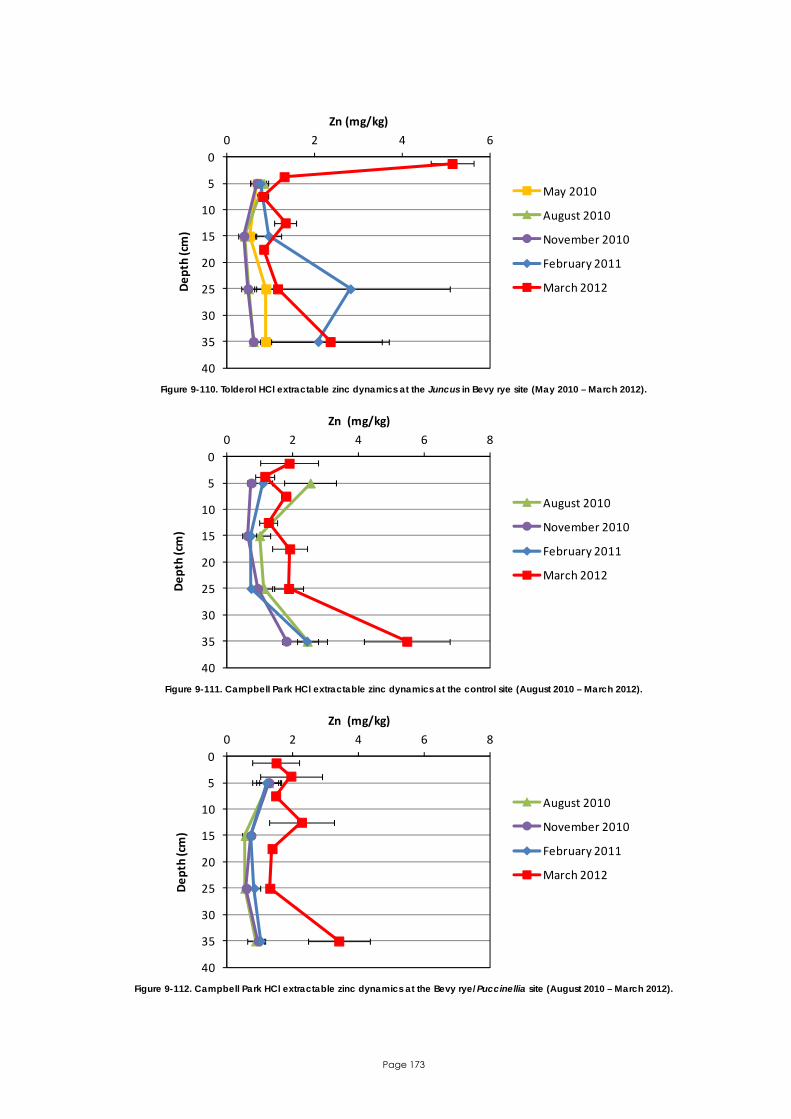
Page 173
0
5
10
15
20
25
30
35
40
0 2 4 6
Depth (cm)
Zn (mg/kg)
May 2010
August 2010
November 2010
February 2011
March 2012
Figure 9-110. Tolderol HCl extractable zinc dynamics at the Juncus in Bevy rye site (May 2010 – March 2012).
0
5
10
15
20
25
30
35
40
0 2 4 6 8
Depth (cm)
Zn (mg/kg)
August 2010
November 2010
February 2011
March 2012
Figure 9-111. Campbell Park HCl extractable zinc dynamics at the control site (August 2010 – March 2012).
0
5
10
15
20
25
30
35
40
0 2 4 6 8
Depth (cm)
Zn (mg/kg)
August 2010
November 2010
February 2011
March 2012
Figure 9-112. Campbell Park HCl extractable zinc dynamics at the Bevy rye/Puccinellia site (August 2010 – March 2012).

Page 174
APPENDIX 7. Additional information

Page 175
Figure 9-113. Bathymetry map for the Waltowa study area (Source: DEWNR).

Page 176
Figure 9-114. Bathymetry map for the Poltalloch study area (Source: DEWNR).

Page 177
Figure 9-115. Bathymetry map for the Tolderol study area (Source: DEWNR).

Page 178
Figure 9-116. Bathymetry map for the Campbell Park study area (Source: DEWNR).

Page 179
0
1000
2000
3000
4000
5000
6000
7000
-1.1-1.0-0.9-0.8-0.7-0.6-0.5-0.4-0.3-0.2-0.10.00.10.20.30.40.50.60.70.80.91.0
2004
2005
2006
2007
2008
2009
2010
2011
2012
Salin
ity (EC
)
Wat
er L
evel
(m
AH
D)
_
Year
Water Level
Salinity
Figure 9-117. Lake Alexandrina historical water level and salinity data (Source: DEWNR).
-0.9
-0.8
-0.7
-0.6
-0.5
-0.4
-0.3
-0.2
-0.1
0.0
0.1
0.2
0.3
0.4
0.5
0.6
0.7
0.8
0.9
1.0
2008 2009 2010 2011 2012
Year
Wat
er L
evel
(m
AH
D)
_
0
2000
4000
6000
8000
10000
12000
14000
16000
18000
20000
Salin
ity (EC
)
Water Level
Salinity
Figure 9-118. Lake Albert historical water level and salinity data (Source: DEWNR).

Page 180
www.murrayfutures.sa.gov.au
Email: [email protected]
Phone: 1800 226 709 (free call during normal business hours)
Post: Coorong, Lower Lakes and Murray Mouth Projects Department for Environment and Heritage Reply Paid 1047 ADELAIDE SA 5001
© State of South Australia through the Department for Environment and Heritage. You may copy, distribute, display, download and otherwise freely deal with this publication for any purpose subject to the conditions that you (1) attribute the Department as the copyright owner of this publication and that (2) you obtain the prior written consent of the Department for Environment and Heritage if you wish to modify the work or offer the publication for sale or otherwise use it or any part of it for a commercial purpose. Written requests for permission should be addressed to: Design and Production Manager Department for Environment and Heritage GPO Box 1047 Adelaide SA 5001 Disclaimer While reasonable efforts have been made to ensure the contents of this publication are factually correct, the Department of Environment and Heritage makes no representations and accepts no responsibility for the accuracy, completeness or fitness for any particular purpose of the contents, and shall not be liable for any loss or damage that may be occasioned directly or indirectly through the use of or reliance on the contents of this publication. Reference to any company, product or service in this publication should not be taken as a Departmental endorsement of the company, product or service. The views and opinions expressed in this publication are those of the authors and do not necessarily reflect those of the Australian Government or the Minister for the Environment, Heritage and the Arts or the Minister for Climate Change and Water. Printed on recycled paper Printed on recycled paper FIS ##### September 2012 ISBN ###-#-######-##-#