Lower Bounds on Rate of Convergence of CuttingPlane Methods

Xinhua ZhangDept. of Computing Sciences

University of Albertaxinhua2@ualberta.ca

Ankan SahaDept. of Computer Science

University of Chicagoankans@cs.uchicago.edu

S.V. N. VishwanathanDept. of Statistics and

Dept. of Computer SciencePurdue University

vishy@stat.purdue.edu

Abstract

In a recent paper Joachims [1] presented SVM-Perf, a cutting plane method(CPM) for training linear Support Vector Machines (SVMs) which converges toan ε accurate solution in O(1/ε2) iterations. By tightening the analysis, Teo et al.[2] showed thatO(1/ε) iterations suffice. Given the impressive convergence speedof CPM on a number of practical problems, it was conjectured that these ratescould be further improved. In this paper we disprove this conjecture. We presentcounter examples which are not only applicable for training linear SVMs withhinge loss, but also hold for support vector methods which optimize a multivari-ate performance score. However, surprisingly, these problems are not inherentlyhard. By exploiting the structure of the objective function we can devise an algo-rithm that converges in O(1/

√ε) iterations.

1 IntroductionThere has been an explosion of interest in machine learning over the past decade, much of whichhas been fueled by the phenomenal success of binary Support Vector Machines (SVMs). Driven bynumerous applications, recently, there has been increasing interest in support vector learning withlinear models. At the heart of SVMs is the following regularized risk minimization problem:

minw

J(w) :=λ

2‖w‖2︸ ︷︷ ︸

regularizer

+Remp(w)︸ ︷︷ ︸empirical risk

with Remp(w) :=1

n

n∑i=1

max(0, 1− yi 〈w,xi〉). (1)

Here we assume access to a training set of n labeled examples (xi, yi)ni=1 where xi ∈ Rd and yi ∈−1,+1, and use the square Euclidean norm ‖w‖2 =

∑i w

2i as the regularizer. The parameter λ

controls the trade-off between the empirical risk and the regularizer.

There has been significant research devoted to developing specialized optimizers which minimizeJ(w) efficiently. In an award winning paper, Joachims [1] presented a cutting plane method(CPM)1, SVM-Perf, which was shown to converge to an ε accurate solution of (1) in O(1/ε2) iter-ations, with each iteration requiring O(nd) effort. This was improved by Teo et al. [2] who showedthat their Bundle Method for Regularized Risk Minimization (BMRM) (which encompasses SVM-Perf as a special case) converges to an ε accurate solution in O(nd/ε) time.

While online learning methods are becoming increasingly popular for solving (1), a key advantageof CPM such as SVM-Perf and BMRM is their ability to directly optimize nonlinear multivariateperformance measures such as F1-score, ordinal regression loss, and ROCArea which are widelyused in some application areas. In this case Remp does not decompose into a sum of losses overindividual data points like in (1), and hence one has to employ batch algorithms. Letting ∆(y, y)denote the multivariate discrepancy between the correct labels y := (y1, . . . , yn)> and a candidatelabeling y (to be concretized later), the Remp for the multivariate measure is formulated by [3] as

1In this paper we use the term cutting plane methods to denote specialized solvers employed in machinelearning. While clearly related, they must not be confused with cutting plane methods used in optimization.

1

Remp(w) = maxy∈−1,1n

[∆(y, y) +

1

n

n∑i=1

〈w,xi〉 (yi − yi)

]. (2)

In another award winning paper by Joachims [3], the regularized risk minimization problems corre-sponding to these measures are optimized by using a CPM.

Given the widespread use of CPM in machine learning, it is important to understand their conver-gence guarantees in terms of the upper and lower bounds on the number of iterations needed toconverge to an ε accurate solution. The tightest, O(1/ε), upper bounds on the convergence speed ofCPM is due to Teo et al. [2], who analyzed a restricted version of BMRM which only optimizes overone dual variable per iteration. However, on practical problems the observed rate of convergenceis significantly faster than predicted by theory. Therefore, it had been conjectured that the upperbounds might be further tightened via a more refined analysis. In this paper we construct counterexamples for both decomposable Remp like in equation (1) and non-decomposable Remp like inequation (2), on which CPM require Ω(1/ε) iterations to converge, thus disproving this conjecture2.We will work with BMRM as our prototypical CPM. As Teo et al. [2] point out, BMRM includesmany other CPM such as SVM-Perf as special cases.

Our results lead to the following natural question: Do the lower bounds hold because regularizedrisk minimization problems are fundamentally hard, or is it an inherent limitation of CPM? In otherwords, to solve problems such as (1), does there exist a solver which requires less than O(nd/ε)effort (better in n, d and ε)? We provide partial answers. To understand our contribution one needsto understand the two standard assumptions that are made when proving convergence rates:

• A1: The data points xi lie inside a L2 (Euclidean) ball of radius R, that is, ‖xi‖ ≤ R.• A2: The subgradient of Remp is bounded, i.e., at any point w, there exists a subgradient g

of Remp such that ‖g‖ ≤ G <∞.

Clearly assumption A1 is more restrictive than A2. By adapting a result due to [6] we show that onecan devise anO(nd/

√ε) algorithm for the case when assumption A1 holds. Finding a fast optimizer

under assumption A2 remains an open problem.

Notation: Lower bold case letters (e.g., w, µ) denote vectors, wi denotes the i-th component ofw, 0 refers to the vector with all zero components, ei is the i-th coordinate vector (all 0’s except1 at the i-th coordinate) and ∆k refers to the k dimensional simplex. Unless specified otherwise,〈·, ·〉 denotes the Euclidean dot product 〈x,w〉 =

∑i xiwi, and ‖·‖ refers to the Euclidean norm

‖w‖ := (〈w,w〉)1/2. We denote R := R ∪ ∞, and [t] := 1, . . . , t.Our paper is structured as follows. We briefly review BMRM in Section 2. Two types of lowerbounds are subsequently defined in Section 3, and Section 4 contains descriptions of various counterexamples that we construct. In Section 5 we describe an algorithm which provably converges to anε accurate solution of (1) in O(1/

√ε) iterations under assumption A1. The paper concludes with a

discussion and outlook in Section 6. Technical proofs and a ready reckoner of the convex analysisconcepts used in the paper can be found in the supplementary material.

2 BMRMAt every iteration, BMRM replaces Remp by a piecewise linear lower bound Rcp

k and optimizes [2]

minw

Jk(w) :=λ

2‖w‖2 +Rcp

k (w), where Rcpk (w) := max

1≤i≤k〈w,ai〉+ bi, (3)

to obtain the next iterate wk. Here ai ∈ ∂Remp(wi−1) denotes an arbitrary subgradient of Remp

at wi−1 and bi = Remp(wi−1) − 〈wi−1,ai〉. The piecewise linear lower bound is successivelytightened until the gap

εk := min0≤t≤k

J(wt)− Jk(wk) (4)falls below a predefined tolerance ε.

Since Jk in (3) is a convex objective function, one can compute its dual. Instead of minimizing Jkwith respect to w one can equivalently maximize the dual [2]:

Dk(α) = − 1

2λ‖Akα‖2 + 〈bk,α〉 , (5)

2Because of the specialized nature of these solvers, lower bounds for general convex optimizers such asthose studied by Nesterov [4] and Nemirovski and Yudin [5] do not apply.

2

Algorithm 1: qp-bmrm: solving the inner loopof BMRM exactly via full QP.

Require: Previous subgradients aiki=1 andintercepts biki=1.

1: Set Ak :=(a1, . . . ,ak) ,bk :=(b1, . . . bk)>.

2: αk ← argmaxα∈∆k

− 1

2λ‖Akα‖2 + 〈α,bk〉

.

3: return wk = −λ−1Akαk.

Algorithm 2: ls-bmrm: solving the inner loopof BMRM approximately via line search.

Require: Previous subgradients aiki=1 andintercepts biki=1.

1: Set Ak :=(a1, . . . ,ak) ,bk :=(b1, . . . bk)>.2: Set α(η) :=

(ηα>k−1, 1− η

)>.

3: ηk←argmaxη∈[0,1]

−12λ ‖Akα(η)‖2+〈α(η),bk〉

.

4: αk ←(ηkα

>k−1, 1− ηk

)>.

5: return wk = −λ−1Akαk.

and set αk = argmaxα∈∆kDk(α). Note that Ak and bk in (5) are defined in Algorithm 1. Since

maximizing Dk(α) is a quadratic programming (QP) problem, we call this algorithm qp-bmrm.Pseudo-code can be found in Algorithm 1.

Note that at iteration k the dualDk(α) is a QP with k variables. As the number of iterations increasesthe size of the QP also increases. In order to avoid the growing cost of the dual optimization at eachiteration, [2] proposed using a one-dimensional line search to calculate an approximate maximizerαk on the line segment (ηα>k−1, (1−η))> : η ∈ [0, 1], and we call this variant ls-bmrm. Pseudo-code can be found in Algorithm 2. We refer the reader to [2] for details.

Even though qp-bmrm solves a more expensive optimization problem Dk(α) per iteration, Teoet al. [2] could only show that both variants of BMRM converge at O(1/ε) rates:

Theorem 1 ([2]) Suppose assumption A2 holds. Then for any ε < 4G2/λ, both ls-bmrm and qp-bmrm converge to an ε accurate solution of (1) as measured by (4) after at most the followingnumber of steps:

log2

λJ(0)

G2+

8G2

λε− 1.

Generality of BMRM Thanks to the formulation in (3) which only uses Remp, BMRM is applica-ble to a wide variety ofRemp. For example, when used to train binary SVMs withRemp specified by(1), it yields exactly the SVM-Perf algorithm [1]. When applied to optimize the multivariate score,e.g. F1-score with Remp specified by (2), it immediately leads to the optimizer given by [3].

3 Upper and Lower BoundsSince most rates of convergence discussed in the machine learning community are upper bounds,it is important to rigorously define the meaning of a lower bound with respect to ε, and to studyits relationship with the upper bounds. At this juncture it is also important to clarify an importanttechnical point. Instead of minimizing the objective function J(w) defined in (1), if we minimize ascaled version cJ(w) this scales the approximation gap (4) by c. Assumptions such as A1 and A2fix this degree of freedom by bounding the scale of the objective function.

Given a function f ∈ F and an optimization algorithm A, suppose wk are the iterates producedby the algorithmAwhen minimizing f . Define T (ε; f,A) as the first step index k when wk becomesan ε accurate solution3:

T (ε; f,A) = min k : f(wk)−minw f(w) ≤ ε . (6)

Upper and lower bounds are both properties for a pair of F and A. A function g(ε) is called anupper bound of (F , A) if for all functions f ∈ F and all ε > 0, it takes at most order g(ε) steps forA to reduce the gap to less than ε, i.e.,

(UB) ∀ ε > 0,∀ f ∈ F , T (ε; f,A) ≤ g(ε). (7)

3 The initial point also matters, as in the best case we can just start from the optimal solution. Thus the quan-tity of interest is actually T (ε; f,A) := maxw0 mink : f(wk)−minw f(w) ≤ ε, starting point being w0.However, without loss of generality we assume some pre-specified way of initialization.

3

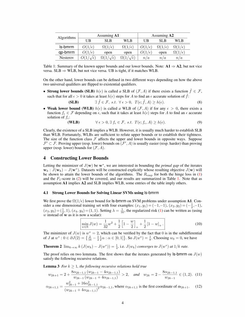
Algorithms Assuming A1 Assuming A2UB SLB WLB UB SLB WLB

ls-bmrm O(1/ε) Ω(1/ε) Ω(1/ε) O(1/ε) Ω(1/ε) Ω(1/ε)

qp-bmrm O(1/ε) open open O(1/ε) open Ω(1/ε)

Nesterov O(1/√ε) Ω(1/

√ε) Ω(1/

√ε) n/a n/a n/a

Table 1: Summary of the known upper bounds and our lower bounds. Note: A1⇒ A2, but not viceversa. SLB⇒WLB, but not vice versa. UB is tight, if it matches WLB.

On the other hand, lower bounds can be defined in two different ways depending on how the abovetwo universal qualifiers are flipped to existential qualifiers.

• Strong lower bounds (SLB) h(ε) is called a SLB of (F , A) if there exists a function f ∈ F ,such that for all ε > 0 it takes at least h(ε) steps for A to find an ε accurate solution of f :

(SLB) ∃ f ∈ F , s.t. ∀ ε > 0, T (ε; f , A) ≥ h(ε). (8)

• Weak lower bound (WLB) h(ε) is called a WLB of (F , A) if for any ε > 0, there exists afunction fε ∈ F depending on ε, such that it takes at least h(ε) steps for A to find an ε accuratesolution of fε:

(WLB) ∀ ε > 0,∃ fε ∈ F , s.t. T (ε; fε, A) ≥ h(ε). (9)

Clearly, the existence of a SLB implies a WLB. However, it is usually much harder to establish SLBthan WLB. Fortunately, WLBs are sufficient to refute upper bounds or to establish their tightness.The size of the function class F affects the upper and lower bounds in opposite ways. SupposeF ′ ⊂ F . Proving upper (resp. lower) bounds on (F ′, A) is usually easier (resp. harder) than provingupper (resp. lower) bounds for (F , A).

4 Constructing Lower BoundsLetting the minimizer of J(w) be w∗, we are interested in bounding the primal gap of the iterateswk : J(wk) − J(w∗). Datasets will be constructed explicitly whose resulting objective J(w) willbe shown to attain the lower bounds of the algorithms. The Remp for both the hinge loss in (1)and the F1-score in (2) will be covered, and our results are summarized in Table 1. Note that asassumption A1 implies A2 and SLB implies WLB, some entries of the table imply others.

4.1 Strong Lower Bounds for Solving Linear SVMs using ls-bmrm

We first prove the Ω(1/ε) lower bound for ls-bmrm on SVM problems under assumption A1. Con-sider a one dimensional training set with four examples: (x1, y1) = (−1,−1), (x2, y2) = (− 1

2 ,−1),(x3, y3)=( 1

2 , 1), (x4, y4)=(1, 1). Setting λ = 116 , the regularized risk (1) can be written as (using

w instead of w as it is now a scalar):

minw∈R

J(w) =1

32w2 +

1

2

[1− w

2

]+

+1

2[1− w]+ . (10)

The minimizer of J(w) is w∗ = 2, which can be verified by the fact that 0 is in the subdifferentialof J at w∗ : 0 ∈ ∂J(2) =

216 −

12

12α : α ∈ [0, 1]

. So J(w∗) = 1

8 . Choosing w0 = 0, we have

Theorem 2 limk→∞ k (J(wk)− J(w∗)) = 14 , i.e. J(wk) converges to J(w∗) at 1/k rate.

The proof relies on two lemmata. The first shows that the iterates generated by ls-bmrm on J(w)satisfy the following recursive relations.

Lemma 3 For k ≥ 1, the following recursive relations hold true

w2k+1 = 2 +8α2k−1,1 (w2k−1 − 4α2k−1,1)

w2k−1 (w2k−1 + 4α2k−1,1)> 2, and w2k = 2− 8α2k−1,1

w2k−1∈ (1, 2). (11)

α2k+1,1 =w2

2k−1 + 16α22k−1,1

(w2k−1 + 4α2k−1,1)2α2k−1,1,where α2k+1,1 is the first coordinate of α2k+1. (12)

4

The proof is lengthy and is relegated to Appendix B. These recursive relations allow us to derive theconvergence rate of α2k−1,1 and wk (see proof in Appendix C):

Lemma 4 limk→∞ kα2k−1,1 = 14 . Combining with (11), we get limk→∞ k|2− wk| = 2.

Now that wk approaches 2 at the rate of O(1/k), it is finally straightforward to translate it into therate at which J(wk) approaches J(w∗). See the proof of Theorem 2 in Appendix D.

4.2 Weak Lower Bounds for Solving Linear SVMs using qp-bmrm

Theorem 1 gives an upper bound on the convergence rate of qp-bmrm, assuming thatRemp satisfiesthe assumption A2. In this section we further demonstrate that thisO(1/ε) rate is also a WLB (hencetight) even when the Remp is specialized to SVM objectives satisfying A2.

Given ε > 0, define n = d1/εe and construct a dataset (xi, yi)ni=1 as yi = (−1)i and xi =(−1)i (nei+1 +

√ne1) ∈ Rn+1. Then the corresponding objective function (1) is

J(w)=‖w‖2

2+Remp(w), where Remp(w)=

1

n

n∑i=1

[1−yi〈w,xi〉]+ =1

n

n∑i=1

[1−√nw1−nwi+1]+.

(13)It is easy to see that the minimizer w∗ = 1

2 ( 1√n, 1n ,

1n , . . . ,

1n )> and J(w∗) = 1

4n . In fact, simply

check that yi 〈w∗,xi〉 = 1, so ∂J(w∗) =

w∗ −

(1√n

∑ni=1 αi, α1, . . . , αn

)>: αi ∈ [0, 1]

, and

setting all αi = 12n yields the subgradient 0. Our key result is the following theorem.

Theorem 5 Let w0 = ( 1√n, 0, 0, . . .)>. Suppose running qp-bmrm on the objective function (13)

produces iterates w1, . . . ,wk, . . .. Then it takes qp-bmrm at least⌊

23ε

⌋steps to find an ε accurate

solution. Formally,mini∈[k]

J(wi)− J(w∗) =1

2k+

1

4nfor all k ∈ [n], hence min

i∈[k]J(wi)− J(w∗) > ε for all k <

2

3ε.

Indeed, after taking n steps, wn will cut a subgradient an+1 = 0 and bn+1 = 0, and then theminimizer of Jn+1(w) gives exactly w∗.

Proof Since Remp(w0) = 0 and ∂Remp(w0) =−1n

∑ni=1 αiyixi : αi ∈ [0, 1]

, we can choose

a1 = − 1

ny1x1 =

(− 1√

n,−1, 0, . . .

)>, b1 = Remp(w0)− 〈a1,w0〉 = 0 +

1

n=

1

n, and

w1 = argminw

1

2‖w‖2 − 1√

nw1 − w2 +

1

n

=

(1√n, 1, 0, . . .

)>.

In general, we claim that the k-th iterate wk produced by qp-bmrm is given by

wk =

(1√n,

k copies︷ ︸︸ ︷1

k, . . . ,

1

k, 0, . . .

)>.

We prove this claim by induction on k. Assume the claim holds true for steps 1, . . . , k, then it iseasy to check that Remp(wk) = 0 and ∂Remp(wk) =

−1n

∑ni=k+1 αiyixi : αi ∈ [0, 1]

. Thus we

can again choose

ak+1 = − 1

nyk+1xk+1, and bk+1 = Remp(wk)− 〈ak+1,wk〉 =

1

n, so

wk+1 = argminw

1

2‖w‖2 + max

1≤i≤k+1〈ai,w〉+ bi

=

(1√n,

k+1 copies︷ ︸︸ ︷1

k + 1, . . . ,

1

k + 1, 0, . . .

)>,

which can be verified by checking that ∂Jk+1(wk+1) =wk+1 +

∑i∈[k+1] αiai : α ∈ ∆k+1

3

0. All that remains is to observe that J(wk) = 12k + 1

2n while J(w∗) = 14n from which it follows

that J(wk)− J(w∗) = 12k + 1

4n as claimed.

5

As an aside, the subgradient of theRemp in (13) does have Euclidean norm√

2n at w = 0. However,in the above run of qp-bmrm, ∂Remp(w0), . . . , ∂Remp(wn) always contains a subgradient withnorm 1. So if we restrict the feasible region to

n−1/2

× [0,∞]n, then J(w) does satisfy the

assumption A2 and the optimal solution does not change. This is essentially a local satisfaction ofA2. In fact, having a bounded subgradient of Remp at all wk is sufficient for qp-bmrm to convergeat the rate in Theorem 1.

However when we assume A1 which is more restrictive than A2, it remains an open question todetermine whether the O(1/ε) rates are optimal for qp-bmrm on SVM objectives. Also left open isthe SLB for qp-bmrm on SVMs.

4.3 Weak Lower Bounds for Optimizing F1-score using qp-bmrm

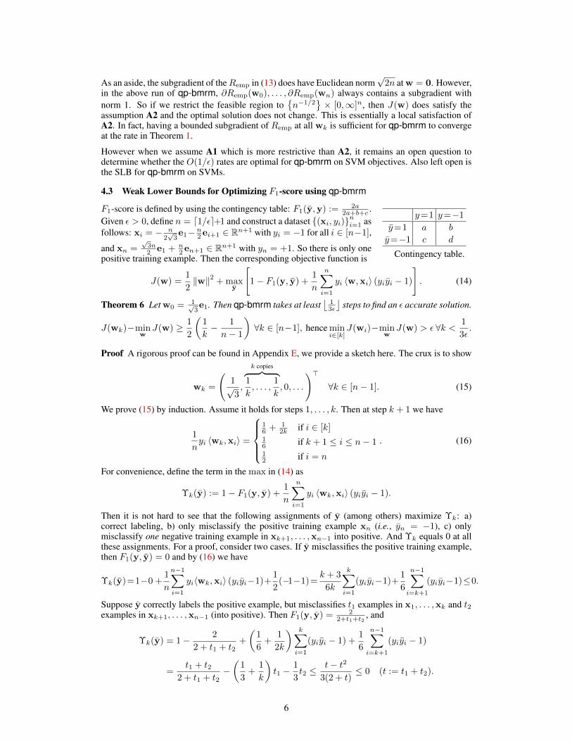
F1-score is defined by using the contingency table: F1(y,y) := 2a2a+b+c .

Given ε > 0, define n = d1/εe+1 and construct a dataset (xi, yi)ni=1 asfollows: xi = − n

2√

3e1− n

2 ei+1 ∈ Rn+1 with yi = −1 for all i ∈ [n−1],

and xn =√

3n2 e1 + n

2 en+1 ∈ Rn+1 with yn = +1. So there is only onepositive training example. Then the corresponding objective function is

y=1 y=−1

y=1 a b

y=−1 c d

Contingency table.

J(w) =1

2‖w‖2 + max

y

[1− F1(y, y) +

1

n

n∑i=1

yi 〈w,xi〉 (yiyi − 1)

]. (14)

Theorem 6 Let w0 = 1√3e1. Then qp-bmrm takes at least

⌊13ε

⌋steps to find an ε accurate solution.

J(wk)−minw

J(w) ≥ 1

2

(1

k− 1

n− 1

)∀k ∈ [n−1], hence min

i∈[k]J(wi)−min

wJ(w) > ε ∀k < 1

3ε.

Proof A rigorous proof can be found in Appendix E, we provide a sketch here. The crux is to show

wk =

(1√3,

k copies︷ ︸︸ ︷1

k, . . . ,

1

k, 0, . . .

)>∀k ∈ [n− 1]. (15)

We prove (15) by induction. Assume it holds for steps 1, . . . , k. Then at step k + 1 we have

1

nyi 〈wk,xi〉 =

16 + 1

2k if i ∈ [k]16 if k + 1 ≤ i ≤ n− 112 if i = n

. (16)

For convenience, define the term in the max in (14) as

Υk(y) := 1− F1(y, y) +1

n

n∑i=1

yi 〈wk,xi〉 (yiyi − 1).

Then it is not hard to see that the following assignments of y (among others) maximize Υk: a)correct labeling, b) only misclassify the positive training example xn (i.e., yn = −1), c) onlymisclassify one negative training example in xk+1, . . . ,xn−1 into positive. And Υk equals 0 at allthese assignments. For a proof, consider two cases. If y misclassifies the positive training example,then F1(y, y) = 0 and by (16) we have

Υk(y)=1−0 +1

n

n−1∑i=1

yi〈wk,xi〉 (yiyi−1)+1

2(−1−1)=

k + 3

6k

k∑i=1

(yiyi−1)+1

6

n−1∑i=k+1

(yiyi−1)≤0.

Suppose y correctly labels the positive example, but misclassifies t1 examples in x1, . . . ,xk and t2examples in xk+1, . . . ,xn−1 (into positive). Then F1(y, y) = 2

2+t1+t2, and

Υk(y) = 1− 2

2 + t1 + t2+

(1

6+

1

2k

) k∑i=1

(yiyi − 1) +1

6

n−1∑i=k+1

(yiyi − 1)

=t1 + t2

2 + t1 + t2−(

1

3+

1

k

)t1 −

1

3t2 ≤

t− t2

3(2 + t)≤ 0 (t := t1 + t2).

6

So we can pick y as (

k copies︷ ︸︸ ︷−1, . . . ,−1,+1,

n−k−1 copies︷ ︸︸ ︷−1, . . . ,−1,+1)> which only misclassifies xk+1, and get

ak+1 =−2

nyk+1xk+1 = − 1√

3e1 − ek+2, bk+1 = Remp(wk)− 〈ak+1,wk〉 = 0 +

1

3=

1

3,

wk+1 = argminw

:=Jk+1(w)︷ ︸︸ ︷1

2‖w‖2 + max

i∈[k+1]〈ai,w〉+ bi =

(1√3,

k+1 copies︷ ︸︸ ︷1

k + 1, . . . ,

1

k + 1, 0, . . .

)>.

which can be verified by ∂Jk+1(wk+1) =wk+1 +

∑k+1i=1 αiai : α ∈ ∆k+1

3 0 (just set all

αi = 1k+1 ). So (15) holds for step k + 1. End of induction.

All that remains is to observe that J(wk) = 12 ( 1

3 + 1k ) while minw J(w) ≤ J(wn−1) = 1

2 ( 13 + 1

n−1 )

from which it follows that J(wk)−minw J(w) ≥ 12 ( 1k −

1n−1 ) as claimed in Theorem 6.

5 An O(nd/√ε) Algorithm for Training Binary Linear SVMs

The lower bounds we proved above show that CPM such as BMRM require Ω(1/ε) iterations toconverge. We now show that this is an inherent limitation of CPM and not an artifact of the problem.To demonstrate this, we will show that one can devise an algorithm for problems (1) and (2) whichwill converge in O(1/

√ε) iterations. The key difficulty stems from the non-smoothness of the

objective function, which renders second and higher order algorithms such as L-BFGS inapplicable.However, thanks to Theorem 11 (see appendix A), the Fenchel dual of (1) is a convex smoothfunction with a Lipschitz continuous gradient, which are easy to optimize.

To formalize the idea of using the Fenchel dual, we can abstract from the objectives (1) and (2) acomposite form of objective functions used in machine learning with linear models:

minw∈Q1

J(w) = f(w) + g?(Aw), where Q1 is a closed convex set. (17)

Here, f(w) is a strongly convex function corresponding to the regularizer, Aw stands for the outputof a linear model, and g? encodes the empirical risk measuring the discrepancy between the correctlabels and the output of the linear model. Let the domain of g be Q2. It is well known that [e.g. 7,Theorem 3.3.5] under some mild constraint qualifications, the adjoint form of J(w):

D(α) = −g(α)− f?(−A>α), α ∈ Q2 (18)

satisfies J(w) ≥ D(α) and infw∈Q1J(w) = supα∈Q2

D(α).

Example 1: binary SVMs with bias. Let A := −Y X> where Y := diag(y1, . . . , yn) and X :=

(x1, . . . ,xn), f(w) = λ2 ‖w‖

2, g?(u) = minb∈R 1n

∑ni=1 [1 + ui − yib]+ which corresponds to

g(α)=−∑i αi. Then the adjoint form turns out to be the well known SVM dual objective function:

D(α) =∑i

αi −1

2λα>Y X>XYα, α ∈ Q2 =

α ∈ [0, n−1]n :

∑i

yiαi = 0. (19)

Example 2: multivariate scores. Denote A as a 2n-by-d matrix where the y-th row is∑ni=1 x

>i (yi − yi) for each y ∈ −1,+1n, f(w) = λ

2 ‖w‖2, g?(u) = maxy

[∆(y, y) + 1

nuy]

which corresponds to g(α) = −n∑

y ∆(y, y)αy, we recover the primal objective (2) for multi-variate performance measure. Its adjoint form is

D(α) =− 1

2λα>AA>α + n

∑y

∆(y, y)αy, α ∈ Q2 =α ∈ [0, n−1]2

n

:∑y

αy =1

n

. (20)

In a series of papers [6, 8, 9], Nesterov developed optimal gradient based methods for minimizingthe composite objectives with primal (17) and adjoint (18). A sequence of wk and αk is producedsuch that under assumption A1 the duality gap J(wk) − D(αk) is reduced to less than ε after atmost k = O(1/

√ε) steps. We refer the readers to [8] for details.

7

5.1 Efficient Projections in Training SV Models with Optimal Gradient Methods

However, applying Nesterov’s algorithm is challenging, because it requires an efficient subroutinefor computing projections onto the set of constraints Q2. This projection can be either an Euclideanprojection or a Bregman projection.

Example 1: binary SVMs with bias. In this case we need to compute the Euclidean projection toQ2 defined by (19), which entails solving a Quadratic Programming problem with a diagonal Hes-sian, many box constraints, and a single equality constraint. We present an O(n) algorithm for thistask in Appendix F. Plugging this into the algorithm described in [8] and noting that all intermediatesteps of the algorithm can be computed in O(nd) time directly yield a O(nd/

√ε) algorithm. A

self-contained description of the algorithm is given in Appendix G.

Example 2: multivariate scores. Since the dimension of Q2 in (20) is exponentially large inn, Euclidean projection is intractable and we resort to Bregman projection. Given a differentiableconvex function F on Q2, a point α, and a direction g, we can define the Bregman projection as:

V (α,g) := argminα∈Q2

F (α)− 〈∇F (α)− g, α〉 .

Scaling up α by a factor of n, we can choose F (α) as the negative entropy F (α) = −∑i αi logαi.

Then the application of the algorithm in [8] will endow a distribution over all possible labelings:

p(y;w) ∝ exp

(c∆(y,y) +

∑i

ai 〈xi,w〉 yi

), where c and ai are constant scalars. (21)

The solver will request the expectation Ey [∑i aixiyi] which in turn requires that marginal distri-

bution of p(yi). This is not as straightforward as in graphical models because ∆(y,y) may notdecompose. Fortunately, for multivariate scores defined by contingency tables, it is possible to com-pute the marginals in O(n2) time by using dynamic programming, and this cost is similar to thealgorithm proposed by [3]. The idea of the dynamic programming can be found in Appendix H.

6 Outlook and ConclusionCPM are widely employed in machine learning especially in the context of structured prediction[16]. While upper bounds on their rates of convergence were known, lower bounds were not studiedbefore. In this paper we set out to fill this gap by exhibiting counter examples on which CPMrequire Ω(1/ε) iterations. This is a fundamental limitation of these algorithms and not an artifactof the problem. We show this by devising an O(1/

√ε) algorithm borrowing techniques from [8].

However, this algorithm assumes that the dataset is contained in a ball of bounded radius (assumptionA1 Section 1). Devising a O(1/

√ε) algorithm under the less restrictive assumption A2 remains an

open problem.

It is important to note that the linear time algorithm in Appendix F is the key to obtaining aO(nd/

√ε) computational complexity for binary SVMs with bias mentioned in section 5.1. How-

ever, this method has been rediscovered independently by many authors (including us), with theearliest known reference to the best of our knowledge being [10] in 1990. Some recent work in op-timization [11] has focused on improving the practical performance, while in machine learning [12]gave an exact projection algorithm in linear time and [13] gave an expected linear time algorithmfor the same problem.

Choosing an optimizer for a given machine learning task is a trade-off between a number of poten-tially conflicting requirements. CPM are one popular choice but there are others. If one is interestedin classification accuracy alone, without requiring deterministic guarantees, then online to batchconversion techniques combined with stochastic subgradient descent are a good choice [17]. Whilethe dependence on ε is still Ω(1/ε) or worse [18], one gets bounds independent of n. However, aswe pointed out earlier, these algorithms are applicable only when the empirical risk decomposesover the examples.

On the other hand, one can employ coordinate descent in the dual as is done in the Sequential Mini-mal Optimization (SMO) algorithm of [19]. However, as [20] show, if the kernel matrix obtained bystacking xi into a matrix X and X>X is not strictly positive definite, then SMO requires O(1/ε)iterations with each iteration costing O(nd) effort. However, when the kernel matrix is strictly pos-itive definite, then one can obtain an O(n2 log(1/ε)) bound on the number of iterations, which hasbetter dependence on ε, but is prohibitively expensive for large n.

8

References[1] T. Joachims. Training linear SVMs in linear time. In Proc. ACM Conf. Knowledge Discovery

and Data Mining (KDD). ACM, 2006.[2] Choon Hui Teo, S. V. N. Vishwanthan, Alex J. Smola, and Quoc V. Le. Bundle methods for

regularized risk minimization. J. Mach. Learn. Res., 11:311–365, January 2010.[3] T. Joachims. A support vector method for multivariate performance measures. In Proc. Intl.

Conf. Machine Learning, pages 377–384, San Francisco, California, 2005. Morgan KaufmannPublishers.

[4] Yurri Nesterov. Introductory Lectures On Convex Optimization: A Basic Course. Springer,2003.

[5] Arkadi Nemirovski and D Yudin. Problem Complexity and Method Efficiency in Optimization.John Wiley and Sons, 1983.

[6] Yurri Nesterov. A method for unconstrained convex minimization problem with the rate ofconvergence O(1/k2). Soviet Math. Docl., 269:543–547, 1983.

[7] J. M. Borwein and A. S. Lewis. Convex Analysis and Nonlinear Optimization: Theory andExamples. CMS books in Mathematics. Canadian Mathematical Society, 2000.

[8] Yurii Nesterov. Excessive gap technique in nonsmooth convex minimization. SIAM J. onOptimization, 16(1):235–249, 2005. ISSN 1052-6234.

[9] Yurii Nesterov. Gradient methods for minimizing composite objective function. TechnicalReport 76, CORE Discussion Paper, UCL, 2007.

[10] P. M. Pardalos and N. Kovoor. An algorithm for singly constrained class of quadratic programssubject to upper and lower bounds. Mathematical Programming, 46:321–328, 1990.

[11] Y.-H. Dai and R. Fletcher. New algorithms for singly linearly constrained quadratic programssubject to lower and upper bounds. Mathematical Programming: Series A and B archive, 106(3):403–421, 2006.

[12] Jun Liu and Jieping Ye. Efficient euclidean projections in linear time. In Proc. Intl. Conf.Machine Learning. Morgan Kaufmann, 2009.

[13] John Duchi, Shai Shalev-Shwartz, Yoram Singer, and Tushar Chandrae. Efficient projectionsonto the `1-ball for learning in high dimensions. In Proc. Intl. Conf. Machine Learning, 2008.

[14] B. Taskar, C. Guestrin, and D. Koller. Max-margin Markov networks. In S. Thrun, L. Saul, andB. Scholkopf, editors, Advances in Neural Information Processing Systems 16, pages 25–32,Cambridge, MA, 2004. MIT Press.

[15] Michael Collins, Amir Globerson, Terry Koo, Xavier Carreras, and Peter Bartlett. Exponenti-ated gradient algorithms for conditional random fields and max-margin markov networks. J.Mach. Learn. Res., 9:1775–1822, 2008.

[16] I. Tsochantaridis, T. Joachims, T. Hofmann, and Y. Altun. Large margin methods for structuredand interdependent output variables. J. Mach. Learn. Res., 6:1453–1484, 2005.

[17] Shai Shalev-Shwartz, Yoram Singer, and Nathan Srebro. Pegasos: Primal estimated sub-gradient solver for SVM. In Proc. Intl. Conf. Machine Learning, 2007.

[18] Alekh Agarwal, Peter L. Bartlett, Pradeep Ravikumar, and Martin Wainwright. Information-theoretic lower bounds on the oracle complexity of convex optimization. In Neural InformationProcessing Systems, 2009.

[19] J. C. Platt. Sequential minimal optimization: A fast algorithm for training support vectormachines. Technical Report MSR-TR-98-14, Microsoft Research, 1998.

[20] Nikolas List and Hans Ulrich Simon. Svm-optimization and steepest-descent line search. InSanjoy Dasgupta and Adam Klivans, editors, Proc. Annual Conf. Computational LearningTheory, LNCS. Springer, 2009.

[21] J.B. Hiriart-Urruty and C. Lemarechal. Convex Analysis and Minimization Algorithms, I andII, volume 305 and 306. Springer-Verlag, 1993.

9

Supplementary Material

A Concepts from Convex Analysis

The following four concepts from convex analysis are used in the paper.

Definition 7 Suppose a convex function f : Rn → R is finite at w. Then a vector g ∈ Rn is calleda subgradient of f at w if, and only if,

f(w′) ≥ f(w) + 〈w′ −w,g〉 for all w′.

The set of all such g vectors is called the subdifferential of f at w, denoted by ∂wf(w). For anyconvex function f , ∂wf(w) must be nonempty. Furthermore if it is a singleton then f is said to bedifferentiable at w, and we use∇f(w) to denote the gradient.

Definition 8 A convex function f : Rn → R is strongly convex with respect to a norm ‖·‖ if thereexists a constant σ > 0 such that f − σ

2 ‖ · ‖2 is convex. σ is called the modulus of strong convexity

of f , and for brevity we will call f σ-strongly convex.

Definition 9 Suppose a function f : Rn → R is differentiable on Q ⊆ Rn. Then f is said to haveLipschitz continuous gradient (l.c.g) with respect to a norm ‖ ·‖ if there exists a constant L such that

‖∇f(w)−∇f(w′)‖ ≤ L‖w −w′‖ ∀ w,w′ ∈ Q.

For brevity, we will call f L-l.c.g.

Definition 10 The Fenchel dual of a function f : Rn → R, is a function f? : Rn → R defined by

f?(w?) = supw∈Rn

〈w,w?〉 − f(w)

Strong convexity and l.c.g are related by Fenchel duality according to the following lemma:

Theorem 11 ([21, Theorem 4.2.1 and 4.2.2])

1. If f : Rn → R is σ-strongly convex, then f? is finite on Rn and f? is 1σ -l.c.g.

2. If f : Rn → R is convex, differentiable on Rn, and L-l.c.g, then f? is 1L -strongly convex.

Finally, the following lemma gives a useful characterization of the minimizer of a convex function.

Lemma 12 ([21, Theorem 2.2.1]) A convex function f is minimized at w∗ if, and only if, 0 ∈∂f(w∗). Furthermore, if f is strongly convex, then its minimizer is unique.

B Proof of Lemma 3

We prove the lemma by induction on k. Obviously, Lemma 3 holds for k = 1. Suppose it holds forindices up to some k − 1 (k ≥ 2). Let p = 2k − 1 (p ≥ 3). Then

Ap =

(−3

4, 0,−1

4, . . . , 0,−1

4

), bp =

(1, 0,

1

2, . . . , 0,

1

2

),

wp = −16Apαp = (−16)

(−3

4αp,1 −

1

4αp,3 −

1

4αp,5 − . . .−

1

4αp,p−2 −

1

4αp,p

)⇒ αp,3 + . . .+ αp,p−2 + αp,p =

wp4− 3αp,1.

So

10

bpαp = αp,1 +1

2αp,3 +

1

2αp,5 + . . .+

1

2αp,p−2 +

1

2αp,p =

1

8wp −

1

2αp,1.

Since wp > 2, so ap+1 = 0, bp+1 = 0. So Ap+1 = (Ap, 0), bp+1 =(bp, 0

). Let αp+1 =

(ηαp, 1− η), then Dp+1(η) = 8η2(Apαp)2 − ηbpαp. So

ηp+1 =bpαp

16 (Apαp)2 =

2wp − 8αp,1w2p

, wp+1 = −16Apαpηp+1 = wpηp+1 = 2− 8αp,1wp

< 2.

(22)

which proves the claim in (11) for even iterates as p+ 1 = 2k.

Since α2,1 = 19 , p ≥ 3, and αk,1 ≥ αk+1,1 due to the update rule of ls-bmrm, we have

8αp,1 ≤8

9< 2 < wp, hence wp+1 > 1. (23)

Next step, since wp+1 ∈ (1, 2), so ap+2 = − 14 , bp+2 = 1

2 , Ap+2 =(Ap, 0,− 1

4

), bp+1 =

(bp, 0,

12

).

Let αp+2(η) = (ηηp+1αt, η(1− ηp+1), 1− η). Then

Ap+2αp+2 = ηηp+1Apαp −1

4(1− η), bp+2αp+2 = ηηp+1bpαp +

1

2(1− η).

Dp+2(η) = 8(Ap+2αp+2)2 − bp+2αp+2

=

(4ηp+1Apαp + 1

)22

η2−(

4ηp+1Apαp + ηp+1bpαp +1

2

)η+const,

where the const means terms independent of η. So

ηp+2 = argminη∈[0,1]

Dp+2(η) =4ηp+1Apαp + ηp+1bpαp + 1

2(4ηp+1Apαp + 1

)2 =w2p + 16α2

p,1

(wp + 4αp,1)2 , (24)

wp+2 = −16Ap+2αp+2 = −16ηp+2ηp+1Apαp + 4(1− ηp+2) = 2 +8αp,1 (wp − 4αp,1)

wp (wp + 4αp,1),

where the last step is by plugging in the expression of ηp+1 in (22) and ηp+2 in (24). Now using(23) we get

wp+2 − 2 =8αp,1(wp − 4αp,1)

wp(wp + 4αp,1)> 0.

C Proof of Lemma 4

The proof is based on (12). Let βk = 1/α2k−1,1, then limk→∞ βk = ∞ becauselimk→∞ α2k−1,1 = 0. Now

limk→∞

kα2k−1,1 =

(limk→∞

1

kα2k−1,1

)−1

=

(limk→∞

βkk

)−1

=

(limk→∞

βk+1 − βk)−1

,

where the last step is by the discrete version of L’Hospital’s rule.

To compute limk→∞ βk+1 − βk we plug the definition βk = 1/α2k−1,1 into (12), which gives:

1

βk+1=

w22k + 16 1

β2k(

w2k + 4 1βk

)2

1

βk⇒ βk+1 − βk = 8

w2kβ2k

w22kβ

2k + 16

= 8w2k

w22k + 16

β2k

.

Since limk→∞ wk = 2 and limk→∞ βk =∞, so

limk→∞

kα2k−1,1 =

(limk→∞

βk+1 − βk)−1

=1

4.

11

D Proof of Theorem 2

Denote δk = 2− wk, then limk→∞ k |δk| = 2 by Theorem 4. So

If δk > 0, then J(wk)− J(w∗) = 132 (2− δk)2 + 1

2δk2 −

18 = 1

8δk + 132δ

2k = 1

8 |δk|+132δ

2k.

If δk ≤ 0, then J(wk)− J(w∗) = 132 (2− δk)2 − 1

8 = − 18δk + 1

32δ2k = 1

8 |δk|+132δ

2k.

Combining these two cases, we conclude limk→∞ k(J(wk)− J(w∗)) = 14 .

E Proof of Theorem 6

The crux of the proof is to show that

wk =

(1√3,

k copies︷ ︸︸ ︷1

k, . . . ,

1

k, 0, . . .

)>∀k ∈ [n− 1]. (25)

At the first iteration, we have

1

nyi 〈w0,xi〉 =

16 if i ∈ [n− 1]12 if i = n

. (26)

For convenience, define the term in the max of (14) as

Υ0(y) := 1− F1(y, y) +1

n

n∑i=1

yi 〈w0,xi〉 (yiyi − 1).

The key observation in the context of F1 score is that Υ0(y) is maximized at any of the followingassignments of (y1, . . . , yn), and it is easy to check that they all give Υ0(y) = 0:

(−1, . . . ,−1,+1), (−1, . . . ,−1,−1), (+1,−1,−1, . . . ,−1,+1), . . . , (−1, . . . ,−1,+1,+1).

The first assignment is just the correct labeling of the training examples. The second assignment justmisclassifies the only positive example xn into negative. The rest n−1 assignments only misclassifya single negative example into positive. To prove that they maximize Υ0(y), consider two cases ofy. First the positive training example is misclassified. Then F1(y, y) = 0 and by (26) we have

Υ0(y) = 1− 0 +1

n

n−1∑i=1

yi 〈w0,xi〉 (yiyi − 1) +1

2(−1− 1) =

1

6

n−1∑i=1

(yiyi − 1) ≤ 0.

Second, consider the case of y where the positive example is correctly labeled, while t ≥ 1 negativeexamples are misclassified. Then F1(y, y) = 2

2+t , and

Υ0(y) = 1− 2

2 + t+

1

6

n−1∑i=1

(yiyi − 1) =t

2 + t− 1

3t =

t− t2

3(2 + t)≤ 0, ∀t ∈ [1, n− 1].

So now suppose we picky1 = (+1,−1,−1, . . . ,−1,+1)>,

i.e. just misclassify the first negative training example. Then

a1 =−2

ny1x1 =

(− 1√

3,−1, 0, . . .

)>, b1 = Remp(w0)− 〈a1,w0〉 = 0 +

1

3=

1

3,

w1 = argminw

1

2‖w‖2 − 1√

3w1 − w2

=

(1√3, 1, 0, . . .

)>.

Next, we prove (25) by induction. Assume that it holds for steps 1, . . . , k. Then at step k + 1 it iseasy to check that

1

nyi 〈wk,xi〉 =

16 + 1

2k if i ∈ [k]16 if k + 1 ≤ i ≤ n− 112 if i = n

. (27)

12

Define

Υk(y) := 1− F1(y, y) +1

n

n∑i=1

yi 〈wk,xi〉 (yiyi − 1).

Then it is not hard to see that the following y (among others) maximize Υk: a) correct labeling, b)only misclassify the positive training example xn, c) only misclassify one negative training examplein xk+1, . . . ,xn−1. And Υk equals 0 at all these assignments. For proof, again consider two cases.If y misclassifies the positive training example, then F1(y, y) = 0 and by (27) we have

Υk(y) = 1− 0 +1

n

n−1∑i=1

yi 〈wk,xi〉 (yiyi − 1) +1

2(−1− 1)

=

(1

6+

1

2k

) k∑i=1

(yiyi − 1) +1

6

n−1∑i=k+1

(yiyi − 1) ≤ 0.

If y correctly labels the positive example, but misclassifies t1 examples in x1, . . . ,xk and t2 exam-ples in xk+1, . . . ,xn−1 (into positive). Then F1(y, y) = 2

2+t1+t2, and

Υk(y) = 1− 2

2 + t1 + t2+

(1

6+

1

2k

) k∑i=1

(yiyi − 1) +1

6

n−1∑i=k+1

(yiyi − 1)

=t1 + t2

2 + t1 + t2−(

1

3+

1

k

)t1 −

1

3t2 ≤

t− t2

3(2 + t)≤ 0 (t := t1 + t2).

So we can pick y as (

k copies︷ ︸︸ ︷−1, . . . ,−1,+1,

n−k−1 copies︷ ︸︸ ︷−1, . . . ,−1,+1)> which only misclassifies xk+1, and get

ak+1 =−2

nyk+1xk+1 = − 1√

3e1 − ek+2, bk+1 = Remp(wk)− 〈ak+1,wk〉 = 0 +

1

3=

1

3,

wk+1 = argminw

1

2‖w‖2 + max

i∈[k+1]〈ai,w〉+ bi =

(1√3,

k+1 copies︷ ︸︸ ︷1

k + 1, . . . ,

1

k + 1, 0, . . .

)>.

which can be verified by ∂Jk+1(wk+1) =wk+1 +

∑k+1i=1 αiai : α ∈ ∆k+1

3 0 (setting all

αi = 1k+1 ). All that remains is to observe that J(wk) = 1

2 ( 13 + 1

k ) while minw J(w) ≤ J(wn−1) =12 ( 1

3 + 1n−1 ) from which it follows that J(wk)−minw J(w) ≥ 1

2 ( 1k −

1n−1 ) as claimed by Theorem

6.

F A linear time algorithm for a box constrained diagonal QP with a singlelinear equality constraint

It can be shown that the dual optimization problem D(α) from (1) can be reduced into a box con-strained diagonal QP with a single linear equality constraint.

In this section, we focus on the following simple QP:

min1

2

n∑i=1

d2i (αi −mi)

2

s.t. li ≤αi ≤ ui ∀i ∈ [n];n∑i=1

σiαi = z.

Without loss of generality, we assume li < ui and di 6= 0 for all i. Also assume σi 6= 0 becauseotherwise αi can be solved independently. To make the feasible region nonempty, we also assume∑

i

σi(δ(σi > 0)li + δ(σi < 0)ui) ≤ z ≤∑i

σi(δ(σi > 0)ui + δ(σi < 0)li).

13

The algorithm we describe below stems from [10] and finds the exact optimal solution inO(n) time,faster than the O(n log n) complexity in [13].

With a simple change of variable βi = σi(αi −mi), the problem is simplified as

min1

2

n∑i=1

d2iβ

2i

s.t. l′i ≤βi ≤ u′i ∀i ∈ [n];n∑i=1

βi = z′,

where

l′i =

σi(li −mi) if σi > 0

σi(ui −mi) if σi < 0,

u′i =

σi(ui −mi) if σi > 0

σi(li −mi) if σi < 0,

d2i =

d2i

σ2i

, z′ = z −∑i

σimi.

We derive its dual via the standard Lagrangian.

L =1

2

∑i

d2iβ

2i −

∑i

ρ+i (βi − l′i) +

∑i

ρ−i (βi − u′i)− λ

(∑i

βi − z′).

Taking derivative:

∂L

∂βi= d2

iβi − ρ+i + ρ−i − λ = 0 ⇒ βi = d−2

i (ρ+i − ρ

−i + λ). (28)

Substituting into L, we get the dual optimization problem

minD(λ, ρ+i , ρ

−i ) =

1

2

∑i

d−2i (ρ+

i − ρ−i + λ)2 −

∑i

ρ+i l′i +∑i

ρ+i u′i − λz′

s.t. ρ+i ≥ 0, ρ−i ≥ 0 ∀i ∈ [n].

Taking derivative of D with respect to λ, we get:∑i

d−2i (ρ+

i − ρ−i + λ)− z′ = 0. (29)

The KKT condition gives:

ρ+i (βi − l′i) = 0, (30a)

ρ−i (βi − u′i) = 0. (30b)

Now we enumerate four cases.

1. ρ+i > 0, ρ−i > 0. This implies that l′i = βi = u′i, which is contradictory to our assumption.

2. ρ+i = 0, ρ−i = 0. Then by (28), βi = d−2

i λ ∈ [l′i, u′i], hence λ ∈ [d2

i l′i, d

2iu′i].

3. ρ+i > 0, ρ−i = 0. Now by (30) and (28), we have l′i = βi = d−2

i (ρ+i + λ) > d−2

i λ, henceλ < d2

i l′i and ρ+

i = d2i l′i − λ.

4. ρ+i = 0, ρ−i > 0. Now by (30) and (28), we have u′i = βi = d−2

i (−ρ−i + λ) < d−2i λ, hence

λ > d2iu′i and ρ−i = −d2

iu′i + λ.

In sum, we have ρ+i = [d2

i l′i − λ]+ and ρ−i = [λ− d2

iu′i]+. Now (29) turns into

14

λd2i l′i d2i u

′i

l′i

u′i

slope = d−2i

hi(λ)

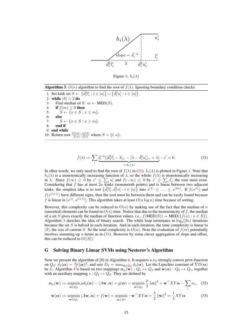
Figure 1: hi(λ)

Algorithm 3: O(n) algorithm to find the root of f(λ). Ignoring boundary condition checks.

1: Set kink set S ←d2i l′i : i ∈ [n]

∪d2iu′i : i ∈ [n]

.

2: while |S| > 2 do3: Find median of S: m← MED(S).4: if f(m) ≥ 0 then5: S ← x ∈ S : x ≤ m.6: else7: S ← x ∈ S : x ≥ m.8: end if9: end while

10: Return root lf(u)−uf(l)f(u)−f(l) where S = l, u.

f(λ) :=∑i

d−2i ([d2

i l′i − λ]+ − [λ− d2

iu′i]+ + λ)︸ ︷︷ ︸

=:hi(λ)

−z′ = 0. (31)

In other words, we only need to find the root of f(λ) in (31). hi(λ) is plotted in Figure 1. Note thathi(λ) is a monotonically increasing function of λ, so the whole f(λ) is monotonically increasingin λ. Since f(∞) ≥ 0 by z′ ≤

∑i u′i and f(−∞) ≤ 0 by z′ ≥

∑i l′i, the root must exist.

Considering that f has at most 2n kinks (nonsmooth points) and is linear between two adjacentkinks, the simplest idea is to sort

d2i l′i, d

2iu′i : i ∈ [n]

into s(1) ≤ . . . ≤ s(2n). If f(s(i)) and

f(s(i+1)) have different signs, then the root must lie between them and can be easily found becausef is linear in [s(i), s(i+1)]. This algorithm takes at least O(n log n) time because of sorting.

However, this complexity can be reduced to O(n) by making use of the fact that the median of n(unsorted) elements can be found inO(n) time. Notice that due to the monotonicity of f , the medianof a set S gives exactly the median of function values, i.e., f(MED(S)) = MED(f(x) : x ∈ S).Algorithm 3 sketches the idea of binary search. The while loop terminates in log2(2n) iterationsbecause the set S is halved in each iteration. And in each iteration, the time complexity is linear to|S|, the size of current S. So the total complexity is O(n). Note the evaluation of f(m) potentiallyinvolves summing up n terms as in (31). However by some clever aggregation of slope and offset,this can be reduced to O(|S|).

G Solving Binary Linear SVMs using Nesterov’s Algorithm

Now we present the algorithm of [8] in Algorithm 4. It requires a σ2-strongly convex prox-functionon Q2: d2(α) = σ2

2 ‖α‖2, and sets D2 = maxα∈Q2

d2(α). Let the Lipschitz constant of ∇D(α)be L. Algorithm 4 is based on two mappings αµ(w) : Q1 7→ Q2 and w(α) : Q2 7→ Q1, togetherwith an auxiliary mapping v : Q2 7→ Q2. They are defined by

αµ(w) := argminα∈Q2

µd2(α)− 〈Aw,α〉+ g(α) = argminα∈Q2

µ

2‖α‖2 + w>XYα−

∑i

αi, (32)

w(α) := argminw∈Q1

〈Aw,α〉+ f(w) = argminw∈Rd

−w>XYα +λ

2‖w‖2 =

1

λXYα (33)

15

Algorithm 4: Solving Binary Linear SVMs using Nesterov’s Algorithm.Require: L as a conservative estimate of (i.e., no less than) the Lipschitz constant of∇D(α).Ensure: Two sequences wk and αk which reduce the duality gap at O(1/k2) rate.

1: Initialize: Randomly pick α−1 in Q2. Let µ0 = 2L, α0 ← v(α−1), w0 ← w(α−1).2: for k = 0, 1, 2, . . . do3: Let τk = 2

k+3 , βk ← (1− τk)αk + τkαµk(wk).

4: Set wk+1 ← (1− τk)wk + τkw(βk), αk+1 ← v(βk), µk+1 ← (1− τk)µk.5: end for

v(α) := argminα′∈Q2

L

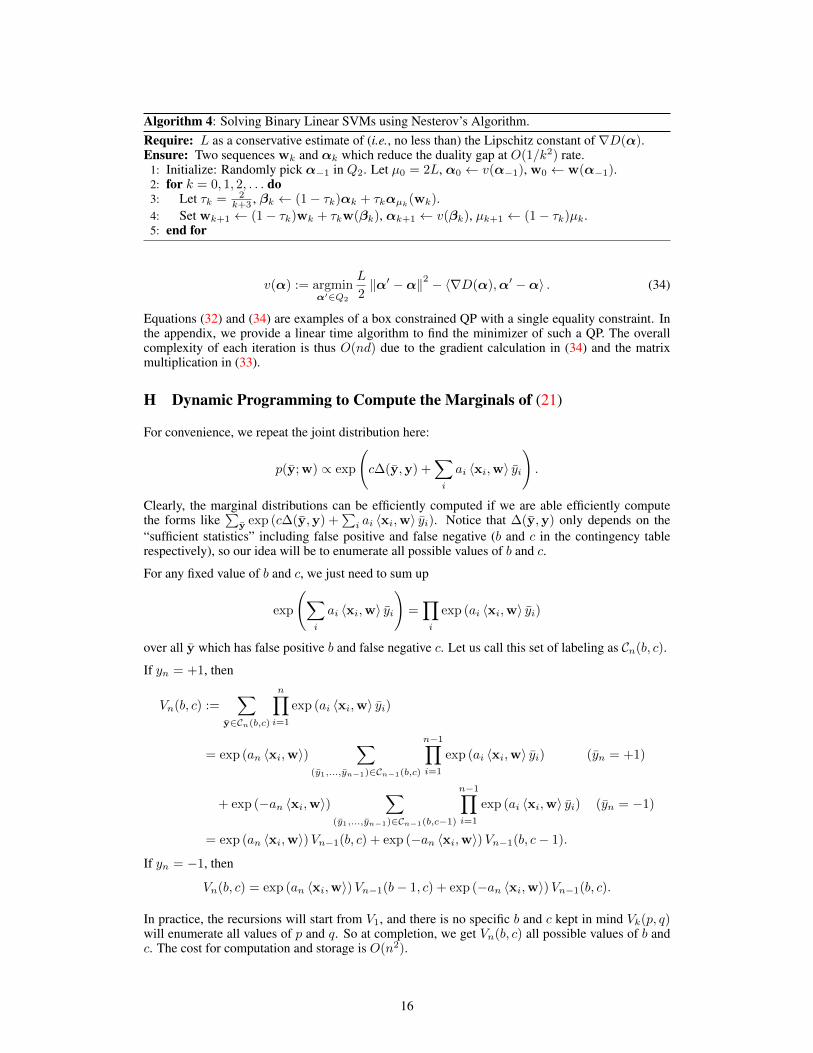
2‖α′ −α‖2 − 〈∇D(α),α′ −α〉 . (34)

Equations (32) and (34) are examples of a box constrained QP with a single equality constraint. Inthe appendix, we provide a linear time algorithm to find the minimizer of such a QP. The overallcomplexity of each iteration is thus O(nd) due to the gradient calculation in (34) and the matrixmultiplication in (33).

H Dynamic Programming to Compute the Marginals of (21)

For convenience, we repeat the joint distribution here:

p(y;w) ∝ exp

(c∆(y,y) +

∑i

ai 〈xi,w〉 yi

).

Clearly, the marginal distributions can be efficiently computed if we are able efficiently computethe forms like

∑y exp (c∆(y,y) +

∑i ai 〈xi,w〉 yi). Notice that ∆(y,y) only depends on the

“sufficient statistics” including false positive and false negative (b and c in the contingency tablerespectively), so our idea will be to enumerate all possible values of b and c.

For any fixed value of b and c, we just need to sum up

exp

(∑i

ai 〈xi,w〉 yi

)=∏i

exp (ai 〈xi,w〉 yi)

over all y which has false positive b and false negative c. Let us call this set of labeling as Cn(b, c).

If yn = +1, then

Vn(b, c) :=∑

y∈Cn(b,c)

n∏i=1

exp (ai 〈xi,w〉 yi)

= exp (an 〈xi,w〉)∑

(y1,...,yn−1)∈Cn−1(b,c)

n−1∏i=1

exp (ai 〈xi,w〉 yi) (yn = +1)

+ exp (−an 〈xi,w〉)∑

(y1,...,yn−1)∈Cn−1(b,c−1)

n−1∏i=1

exp (ai 〈xi,w〉 yi) (yn = −1)

= exp (an 〈xi,w〉)Vn−1(b, c) + exp (−an 〈xi,w〉)Vn−1(b, c− 1).

If yn = −1, then

Vn(b, c) = exp (an 〈xi,w〉)Vn−1(b− 1, c) + exp (−an 〈xi,w〉)Vn−1(b, c).

In practice, the recursions will start from V1, and there is no specific b and c kept in mind Vk(p, q)will enumerate all values of p and q. So at completion, we get Vn(b, c) all possible values of b andc. The cost for computation and storage is O(n2).

16