Embed Size (px)
Citation preview
Low-Thrust Trajectory Optimization with Simplified SQP AlgorithmNATHAN L. PARRISH
DANIEL J. SCHEERES
UNIVERSITY OF COLORADO BOULDER
Astrodynamics Specialist Conference, August 2017
https://ntrs.nasa.gov/search.jsp?R=20170007867 2020-03-11T11:06:44+00:00Z
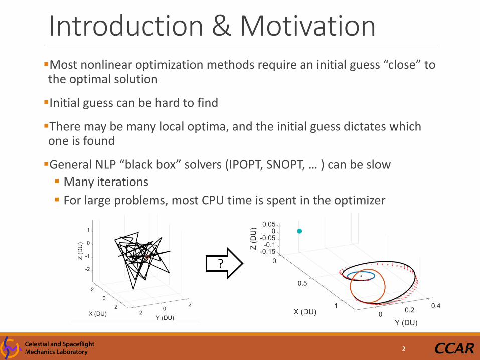
Introduction & MotivationMost nonlinear optimization methods require an initial guess “close” to the optimal solution
Initial guess can be hard to find
There may be many local optima, and the initial guess dictates which one is found
General NLP “black box” solvers (IPOPT, SNOPT, … ) can be slow
Many iterations
For large problems, most CPU time is spent in the optimizer
2
?
Solution OverviewStart with very poor initial guess
Use multiple shooting with ~50-100 nodes Continuous thrust during propagation
Constrain defects to go to zero at matchpoints
Optimize states, controls, and endpoint locations by solving a series of quadratic sub-problems
3
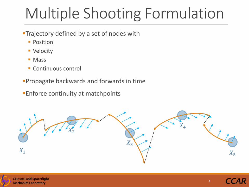
Multiple Shooting FormulationTrajectory defined by a set of nodes with Position
Velocity
Mass
Continuous control
Propagate backwards and forwards in time
Enforce continuity at matchpoints
4
𝑋1
𝑋2
𝑋3
𝑋4
𝑋5
Multiple Shooting FormulationFixed step size integrator is used, with 5 steps per node
Why fixed step size? More consistent finite-differenced partial derivatives faster
convergence
Faster integration (don’t get stuck at a singularity with poor initial guess)
Better for parallelization (future work)
Runge-Kutta 78 numerical integration is used Normally, use the 8th order truncation term to estimate the error in
the 7th order step. Then choose the largest step size possible where the error remains within tolerance.
Here, we force a fixed step size, but use the truncation term to output the error estimate for use in mesh refinement
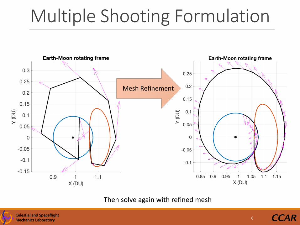
Mesh refinement: Add nodes where the 8th order truncation term for any of the integrator steps is > tolerance
5
Multiple Shooting Formulation
6
Mesh Refinement
Then solve again with refined mesh
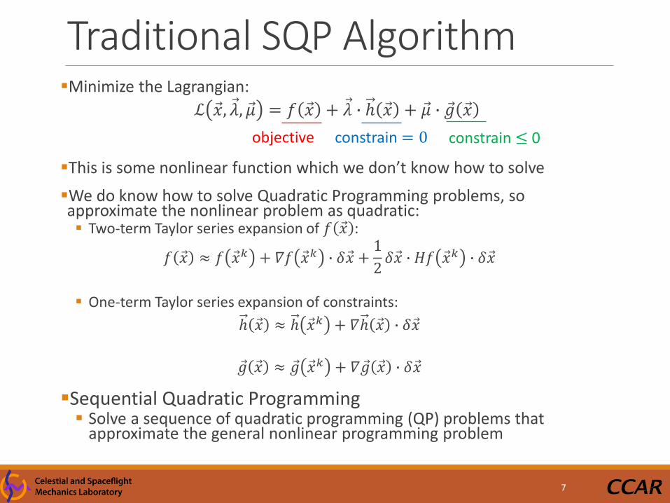
Traditional SQP AlgorithmMinimize the Lagrangian:
ℒ 𝑥, 𝜆, 𝜇 = 𝑓 𝑥 + 𝜆 ∙ ℎ 𝑥 + 𝜇 ∙ 𝑔 𝑥
This is some nonlinear function which we don’t know how to solve
We do know how to solve Quadratic Programming problems, so approximate the nonlinear problem as quadratic: Two-term Taylor series expansion of 𝑓 𝑥 :
𝑓 𝑥 ≈ 𝑓 𝑥𝑘 + 𝛻𝑓 𝑥𝑘 ∙ 𝛿 𝑥 +1
2𝛿 𝑥 ∙ 𝐻𝑓 𝑥𝑘 ∙ 𝛿 𝑥
One-term Taylor series expansion of constraints:
ℎ 𝑥 ≈ ℎ 𝑥𝑘 + 𝛻ℎ 𝑥 ∙ 𝛿 𝑥
𝑔 𝑥 ≈ 𝑔 𝑥𝑘 + 𝛻 𝑔 𝑥 ∙ 𝛿 𝑥
Sequential Quadratic Programming Solve a sequence of quadratic programming (QP) problems that
approximate the general nonlinear programming problem
7
objective constrain = 0 constrain ≤ 0
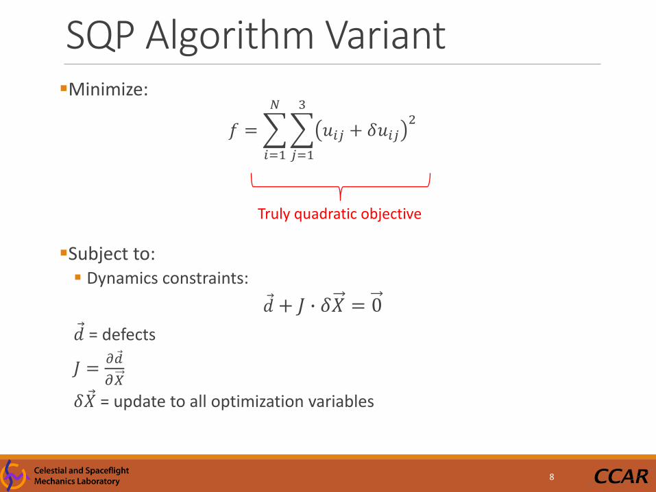
SQP Algorithm VariantMinimize:
𝑓 =
𝑖=1
𝑁
𝑗=1
3
𝑢𝑖𝑗 + 𝛿𝑢𝑖𝑗2
Subject to: Dynamics constraints:
𝑑 + 𝐽 ∙ 𝛿𝑋 = 0 𝑑 = defects
𝐽 =𝜕 𝑑
𝜕𝑋
𝛿 𝑋 = update to all optimization variables
8
Truly quadratic objective
Endpoints
9
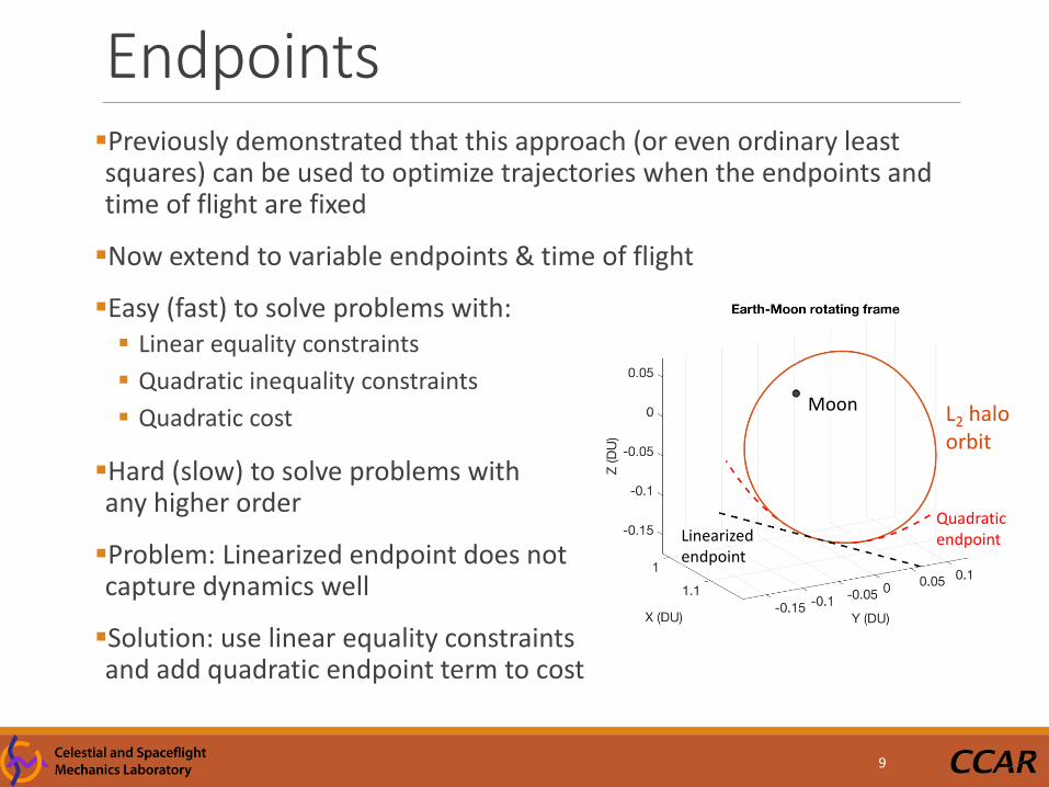
Moon L2 halo orbit
Linearized endpoint
Quadratic endpoint
Previously demonstrated that this approach (or even ordinary least squares) can be used to optimize trajectories when the endpoints and time of flight are fixed
Now extend to variable endpoints & time of flight
Easy (fast) to solve problems with: Linear equality constraints
Quadratic inequality constraints
Quadratic cost
Hard (slow) to solve problems with any higher order
Problem: Linearized endpoint does not capture dynamics well
Solution: use linear equality constraintsand add quadratic endpoint term to cost
Endpoints
10
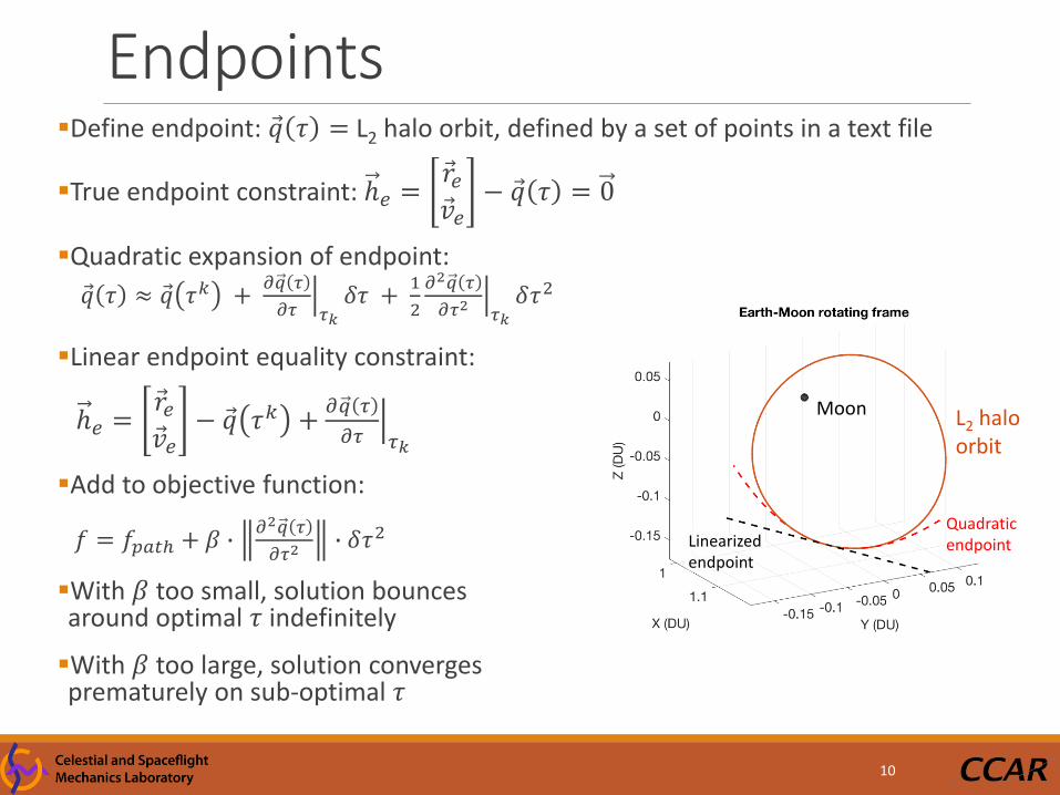
Define endpoint: 𝑞 𝜏 = L2 halo orbit, defined by a set of points in a text file
True endpoint constraint: ℎ𝑒 = 𝑟𝑒 𝑣𝑒
− 𝑞 𝜏 = 0
Quadratic expansion of endpoint:
𝑞 𝜏 ≈ 𝑞 𝜏𝑘 + 𝜕𝑞 𝜏
𝜕𝜏 𝜏𝑘
𝛿𝜏 +1
2
𝜕2𝑞 𝜏
𝜕𝜏2𝜏𝑘
𝛿𝜏2
Linear endpoint equality constraint:
ℎ𝑒 = 𝑟𝑒 𝑣𝑒
− 𝑞 𝜏𝑘 + 𝜕𝑞 𝜏
𝜕𝜏 𝜏𝑘
Add to objective function:
𝑓 = 𝑓𝑝𝑎𝑡ℎ + 𝛽 ∙𝜕2𝑞 𝜏
𝜕𝜏2 ∙ 𝛿𝜏2
With 𝛽 too small, solution bounces around optimal 𝜏 indefinitely
With 𝛽 too large, solution converges prematurely on sub-optimal 𝜏
Moon L2 halo orbit
Linearized endpoint
Quadratic endpoint
Endpoints
11
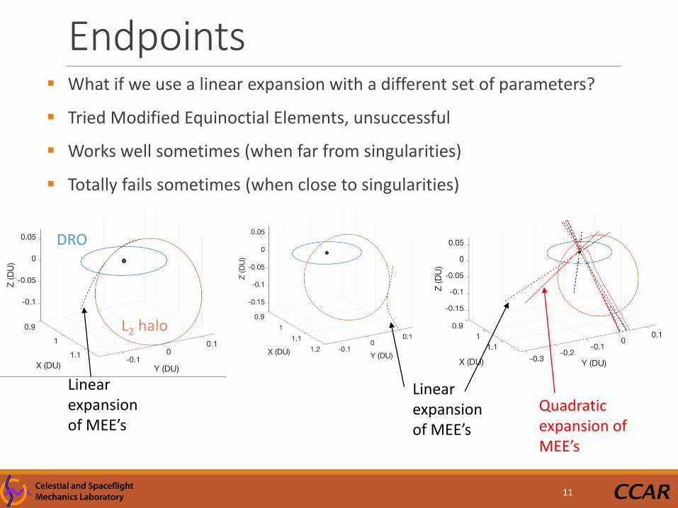
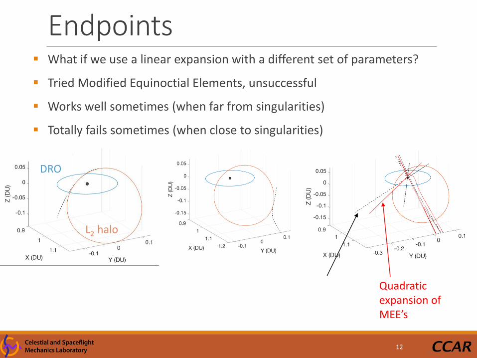
L2 halo
DRO
Linear expansion of MEE’s
Quadratic expansion of MEE’s
Linear expansion of MEE’s
What if we use a linear expansion with a different set of parameters?
Tried Modified Equinoctial Elements, unsuccessful
Works well sometimes (when far from singularities)
Totally fails sometimes (when close to singularities)
Endpoints
12
L2 halo
DRO
Quadratic expansion of MEE’s
What if we use a linear expansion with a different set of parameters?
Tried Modified Equinoctial Elements, unsuccessful
Works well sometimes (when far from singularities)
Totally fails sometimes (when close to singularities)
Line SearchEach solution to the QP problem gives us an update 𝛿 𝑥 to all optimization variables
𝑋𝑘+1 = 𝑋𝑘 + 𝛼 ∙ 𝛿 𝑥
If the problem is sufficiently linear, the QP update is accurate enough to assume 𝛼 = 1
Why do a line search? We do not trust the solution to the linearized problem
𝑋𝑘+1 = 𝑋𝑘 + 𝛼 ∙ 𝛿 𝑥
For short transfers (<1 revolution), no need to perform line search – the problem is sufficiently linear to converge quickly with full steps
13
Maratos effect
Line SearchA comment on parameterization Line search is only necessary as the solution takes on
more revolutions
With a different parameterization (i.e. orbital elements), the revolutions can be “unwound” to keep the problem more linear
However, the optimization algorithm is too “smart” for this Every orbital element set has some singularity (or multiple)
Optimization algorithm will exploit the singularity to find a non-physical solution with very low cost
14
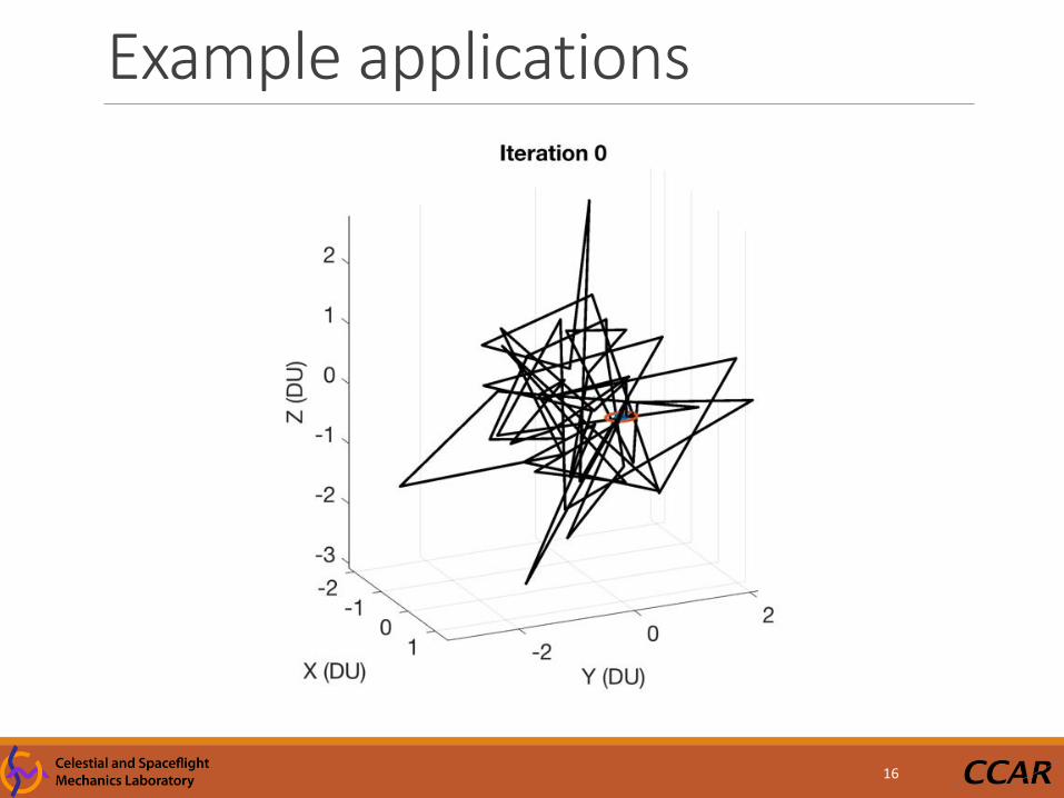
Example applicationsNow, two examples, with CRTBP dynamics DRO (distant retrograde orbit) to L2 halo orbit
DRO to different DRO
Initial guess is random
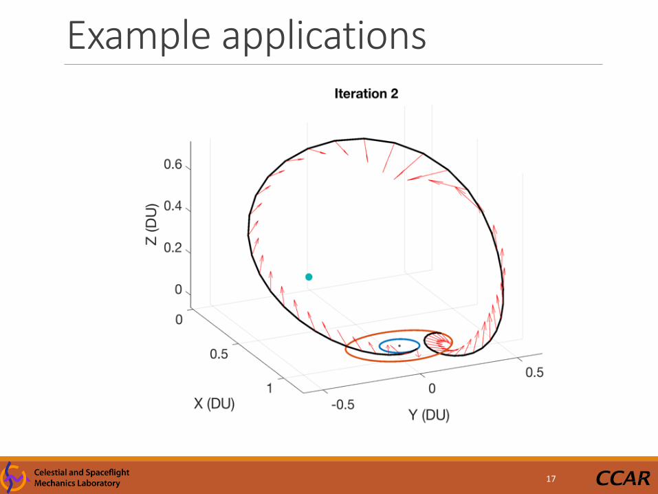
Endpoints and time of flight are variable, but only allowed to change a small amount each iteration, to preserve accuracy of linearization
15
Example applications
16
Example applications
17
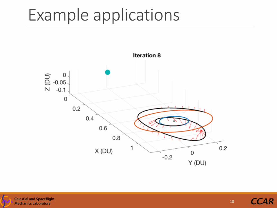
Example applications
18
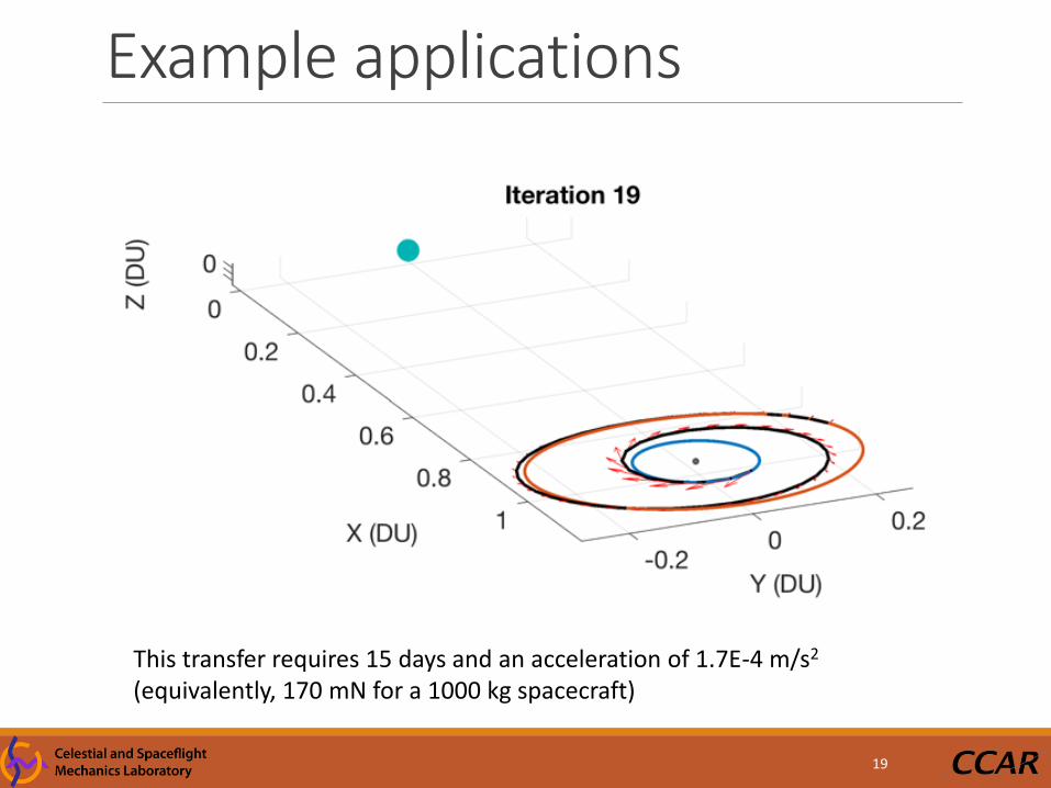
Example applications
19
This transfer requires 15 days and an acceleration of 1.7E-4 m/s2
(equivalently, 170 mN for a 1000 kg spacecraft)
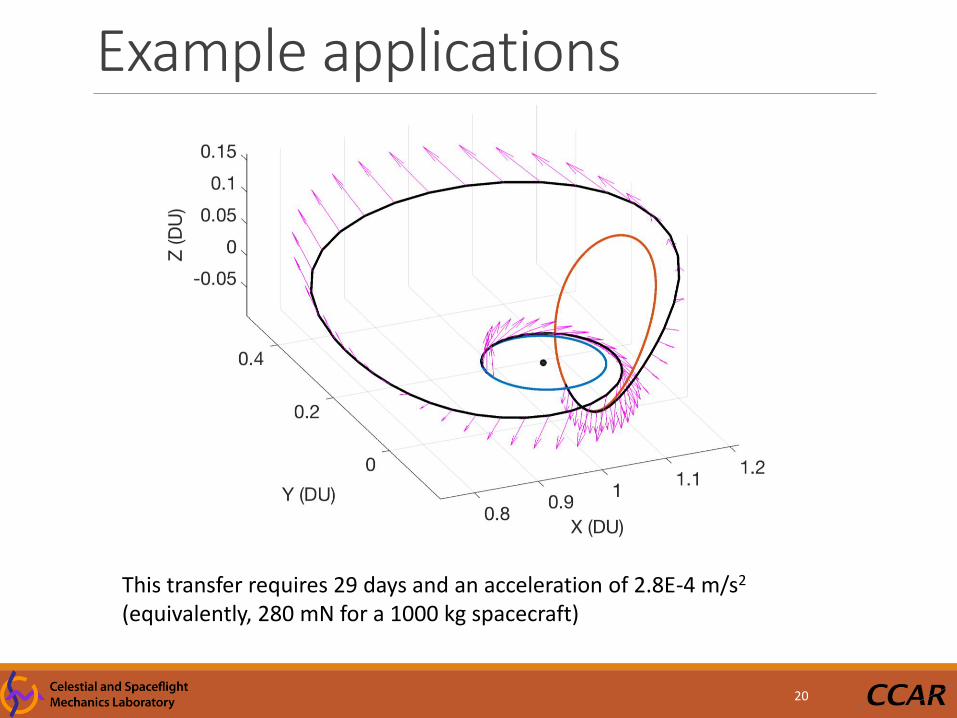
Example applications
20
This transfer requires 29 days and an acceleration of 2.8E-4 m/s2
(equivalently, 280 mN for a 1000 kg spacecraft)
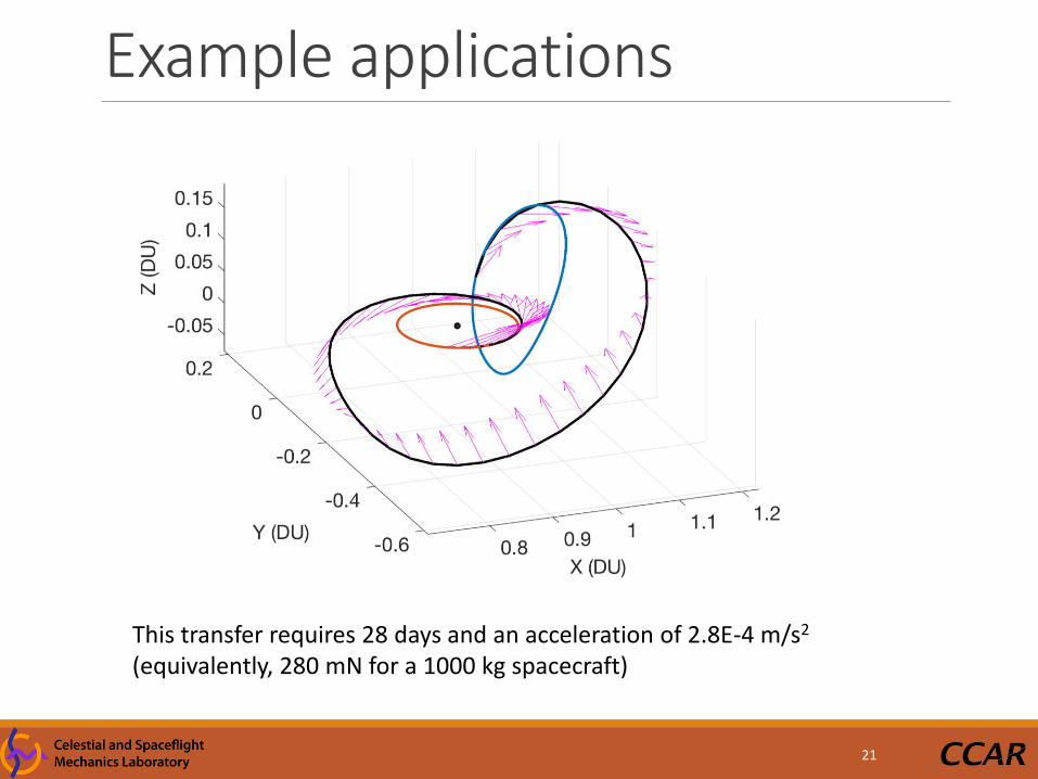
Example applications
21
This transfer requires 28 days and an acceleration of 2.8E-4 m/s2
(equivalently, 280 mN for a 1000 kg spacecraft)
Fuel Optimal Solutions
22
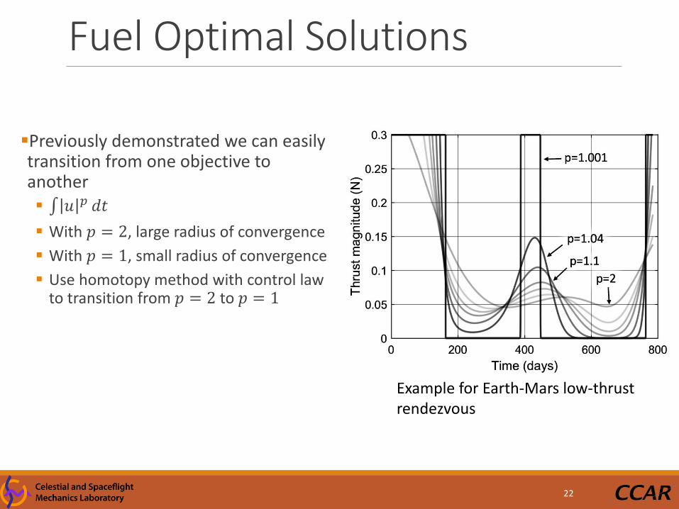
Previously demonstrated we can easily transition from one objective to another 𝑢 𝑝 𝑑𝑡
With 𝑝 = 2, large radius of convergence
With 𝑝 = 1, small radius of convergence
Use homotopy method with control law to transition from 𝑝 = 2 to 𝑝 = 1
Example for Earth-Mars low-thrust rendezvous
Implementation notesImplemented in Julia language, with JuMP optimization toolbox and Gurobi as QP optimizer
Computation time (40-100 nodes): Each iteration: Set up QP problem: 0.2 – 0.5 seconds
Solve QP problem: 0.2 – 0.5 seconds
Line search: 0.2 – 0.5 seconds
Short transfers total time From random initial guess: 10 – 30 seconds
From close initial guess: ~1 – 3 seconds
Long transfers total time varies Line search becomes necessary, so more iterations required
Does not always converge
23
Low-Thrust Trajectory Optimization with Modified SQP Algorithm
Astrodynamics Specialist Conference, August 2017
This work was supported by a NASA Space Technology Research Fellowship
Questions?
NATHAN L. PARRISH
DANIEL J. SCHEERES
UNIVERSITY OF COLORADO BOULDER