LOW-SPEED SINGLE-ELEMENT

AIRFOIL SYNTHESIS

John H. McMasters and Michael L. Henderson

Boeing Commerical Airplane Co.

SUMMARY

Large quantities of experimental data exist on the characteristics of airfoils operating in the Reynolds number range between one and ten million, typical of conventional atmospheric wind tunnel operating conditions. Beyond either end of this range, however, good experimental data becomes scarce. Designers of model airplanes, hang gliders, ultralarge energy efficient transport aircraft, and hio-aerodynamicists attempting to evaluate the performance of natural flying devices are hard pressed to make the kinds of quality performance/design estimates taken for granted by sailplane and general aviation aerodynamicists. Even within the usual range of wind tunnel Reynolds numbers, much of the data is for "smooth" models which give little indication of how a section will perform on a wing of practical construction.

The purpose of this paper is to demonstrate the use of recently developed airfoil analysis/design computational tools to clarify, enrich and extend the existing experimental data base on low-speed, single element airfoils, and then proceed to a discussion of the problem of tailoring an airfoil for a specific application at its appropriate Reynolds number. This latter problem is approached by use of inverse (or "synthesis") techniques, wherein a desirable set of boundary layer characteristics, performance objectives, and constraints are specified, which then leads to derivation of a corresponding viscous flow pressure distribution. In this procedure, the airfoil shape required to produce the desired flow characteristics is only extracted towards the end of the design cycle. This synthesis process is contrasted with the traditional "analysis" (either experimental or computational) approach in which an initial profile shape is selected which then yields a pressure distribution and boundary layer characterisitics, and finally some performance level. The final configuration which provides the required performance is derived by cut-and-try adjustments to the shape.

Examples are presented which demonstrate the synthesis approach, following presentation of some historical information and background data which motivate the basic synthesis process.

INTRODUCTION

Since the dawn of human flight, enormous efforts have been expended on the design of efficient wings and their constituent airfoil sections. As such development became a race for ever increasing speed, the problems of

https://ntrs.nasa.gov/search.jsp?R=19790015719 2018-07-17T16:51:45+00:00Z

low-speed flight frequently became relegated to the status of "off-design" conditions, with performance requirements met by fitting "high speed" cruise airfoils with increasingly complex and sophisticated high-lift devices. During the past forty years, relatively little attention has been given to the development of "optimized" low-speed airfoils by other than academicians and "cut-and-try" experimenters.

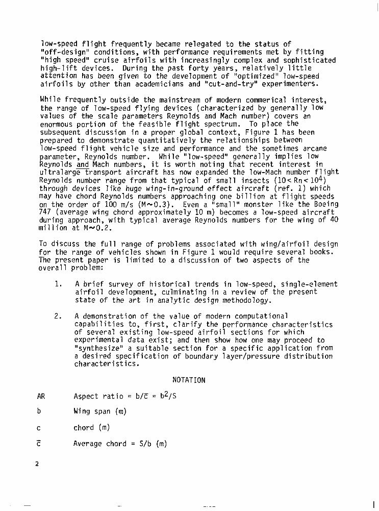
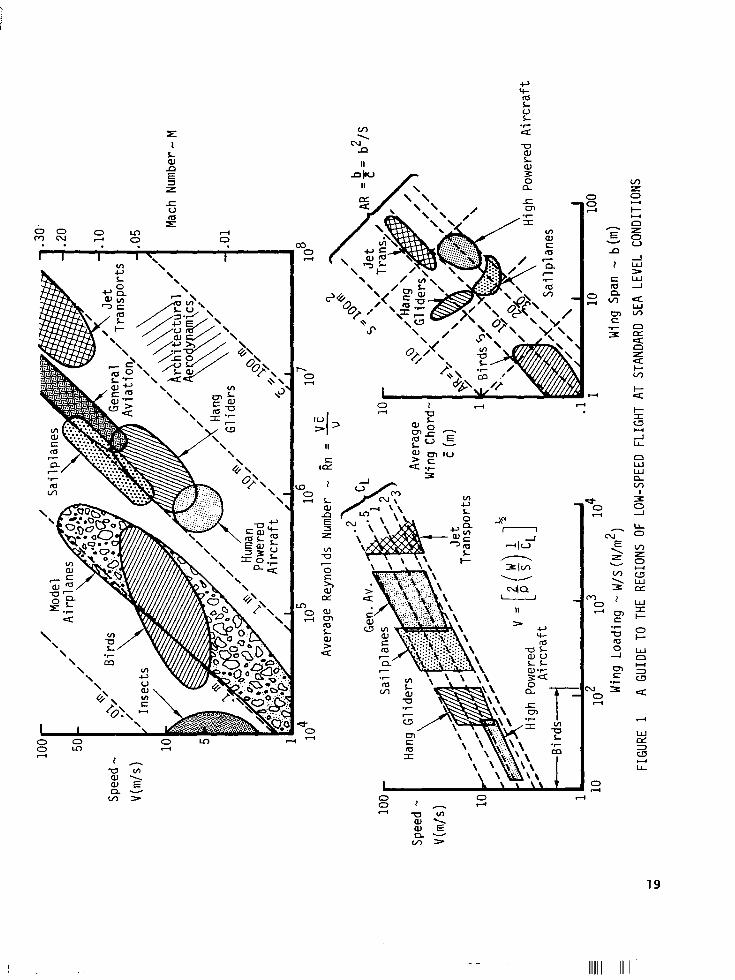
While frequently outside the mainstream of modern commerical interest, the range of low-speed flying devices (characterized by generally 1OW values of the scale parameters Reynolds and Mach number) covers an enormous portion of the feasible flight spectrum. To place the subsequent discussion in a proper global context, Figure 1 has been prepared to demonstrate quantitatively the relationships between low-speed flight vehicle size and performance and the sometimes arcane parameter, Reynolds number. While "low-speed" generally implies low Reynolds and Mach numbers, it is worth noting that recent interest in ultralarge transport aircraft has now expanded the low-Mach number flight Reynolds number range from that typical of small insects (lo< Rnc104) through devices like huge wing-in-ground effect aircraft (ref. 1) which may have chord Reynolds numbers approaching one billion at flight speeds on the order of 100 m/s (M-0.3). Even a "small" monster like the Boeing 747 (average wing chord approximately 10 m) becomes a low-speed aircraft during approach, with typical average Reynolds numbers for the wing of 40 million at Mw0.2.

To discuss the full range of problems associated with wing/airfoil design for the range of vehicles shown in Figure 1 would require several books. The present paper is limited to a discussion of two aspects of the overall problem:

1. A brief survey of historical trends in low-speed, single-element airfoil development, culminating in a review of the present state of the art in analytic design methodology.

2. A demonstration of the value of modern computational capabilities to, first, clarify the performance characteristics of several existing low-speed airfoil sections for which experimental data exist; and then show how one may proceed to "synthesize" a suitable section for a specific application from a desired specification of boundary layer/pressure distribution characteristics.

NOTATION

AR Aspect ratio = b/C = b2/S

b Wing span (m)

C chord (m)

E Average chord = S/b (m)

2

'd

cf

cL

cI1

cP

5ll

H

M

P

9

Rn

S

t

V

Section drag coefficient

Skin friction coefficient

Wing lift coefficient = lift/qS

Section lift coefficient

Pressure coefficient = (p-p,)/q.,

Section pitching moment coefficient

Boundary layer form parameter =6/ 0

Mach number

Static pressure (N/m*)

Dynamic pressure = $pV2 (N/m)

Reynolds number = Vc/u

Wing area (m*)

Airfoil thickness (m)

Velocity (m/s)

Local velocity (m/s)

Weight (N)

Chordwise coordinate

Coordinate normal to chord

Greek symbols:

a Angle of attack (degrees)

6 Boundary layer displacement thickness = I( w 1 . - $-jdz w

Section 1

Boundary

Kinematic

ift-drag ratio = CR /Cd

layer momentum thickness = o SWv( v W 1 - k dz > W

viscosity (1.46 x 1U -5 m*/s standard sea level)

P Air mass density (1.225 kg/m3 standard sea level)

Superscript:

( I* indicates "design condition"

3

Subscript:

( )r recovery point or region

( )tr transition point or "trip" location

1 )fP fair point (see Fig. 9)

( )TE trailing edge

( 100 free-stream condition

( h airfoil upper surface value

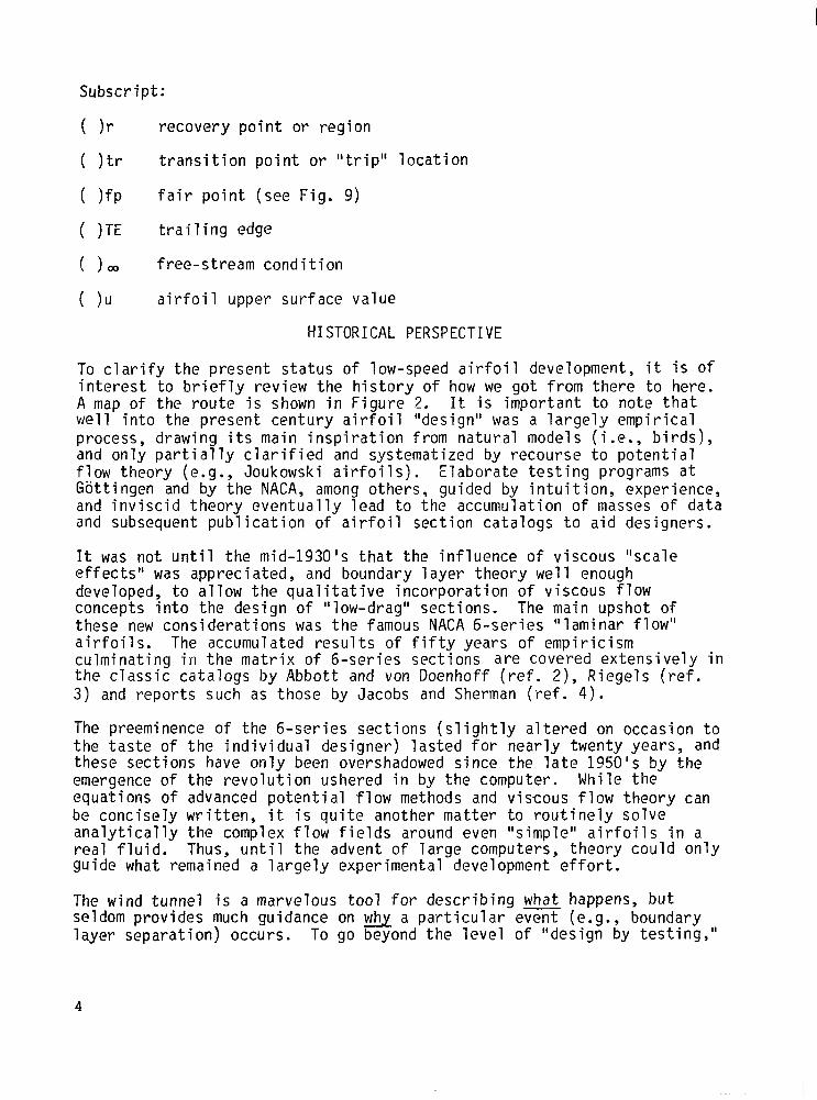
HISTORICAL PERSPECTIVE

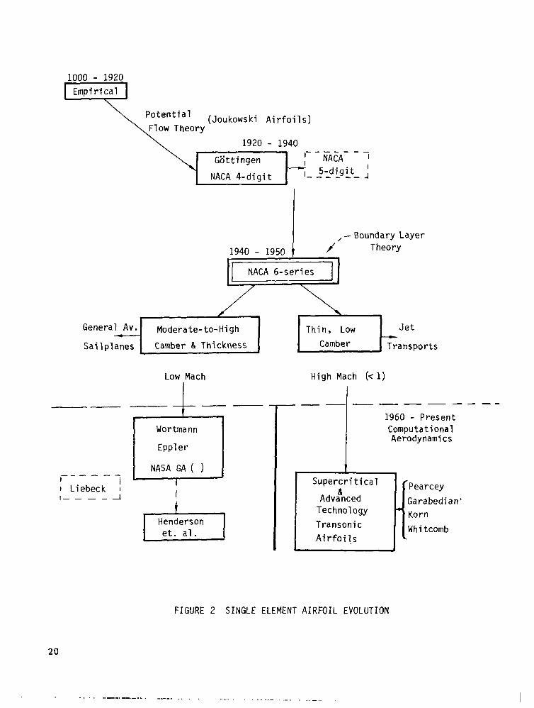
To clarify the present status of low-speed airfoil development, it is of interest to briefly review the history of how we got from there to here. A map of the route is shown in Figure 2. It is important to note that well into the present century airfoil "design" was a largely empirical process, drawing its main inspiration from natural models (i.e., birds), and only partially clarified and systematized by recourse to potential flow theory (e.g., Joukowski airfoils). Elaborate testing programs at Giittingen and by the NACA, among others, guided by intuition, experience, and inviscid theory eventually lead to the accumulation of masses of data and subsequent publication of airfoil section catalogs to aid designers.

It was not until the mid-1930's that the influence of viscous "scale effects" was appreciated, and boundary layer theory well enough developed, to allow the qualitative incorporation of viscous flow concepts into the design of "low-drag" sections. The main upshot of these new considerations was the famous NACA 6-series "laminar flow" airfoils. The accumulated results of fifty years of empiricism culminating in the matrix of 6-series sections are covered extensively in the classic catalogs by Abbott and von Doenhoff (ref. 2), Riegels (ref. 3) and reports such as those by Jacobs and Sherman (ref. 4).

The preeminence of the 6-series sections (slightly altered on occasion to the taste of the individual designer) lasted for nearly twenty years, and these sections have only been overshadowed since the late 1950's by the emergence of the revolution ushered in by the computer. While the equations of advanced potential flow methods and viscous flow theory can be concisely written, it is quite another matter to routinely solve analytically the complex flow fields around even "simple" airfoils in a real fluid. Thus, until the advent of large computers, theory could only guide what remained a largely experimental development effort.

The wind tunnel is a marvelous tool for describing what happens, but seldom provides much guidance on why a particular event (e.g., boundary layer separation) occurs. To go beyond the level of "design by testing,"

4

practical quantitative solutions to the equations of viscous flow were required to supplement empirical experience.

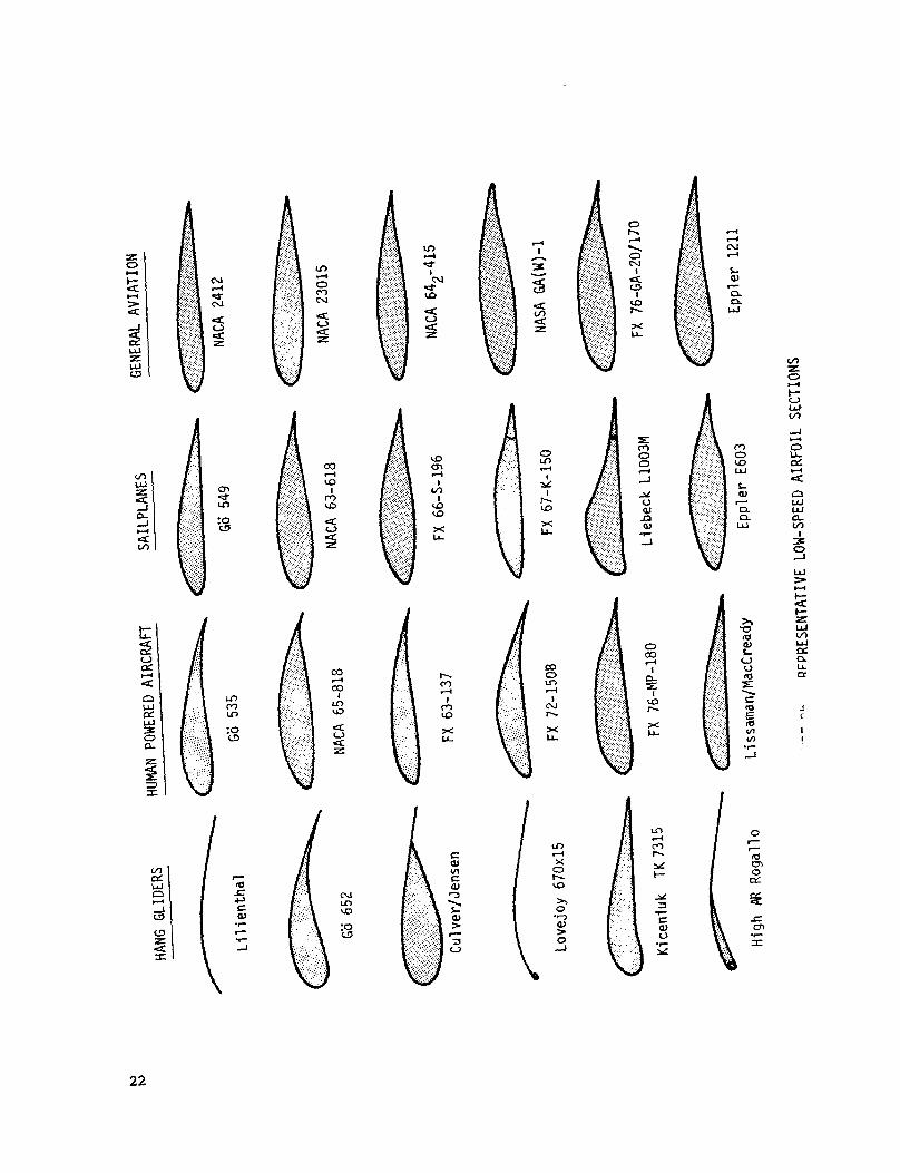
The remarkable success of computer based methods in improving airfoil performance beyond the NACA 6-series level is well demonstrated in the Catalog of Wortmann FX-series sections (ref. 5) and the reports and papers listed in refs. 6 and 7. Despite this new progress, designers without access to a computer of sufficient size, or those lacking a sophisticated background in theoretical aerodynamics and mathematics are still forced to rely on catalog data and outmoded "simplified" theory. With very few exceptions (notably ref. 8), available good catalog data is for "ideal" surface quality wind tunnel models operating in the range 7 x 105 I Rn < 107. As a summary of the preceding historical discussion, Figure 3 shows some representative airfoils sections used, or specifically designed for, various categories of low-speed aircraft during the last eighty years. The variety of shapes even within a given category is sometimes bewildering.

LOW-SPEED AIRFOIL DESIGN

The general principles of low-speed, single-element airfoil design in light of modern theory have been discussed in detail by several authors, notably Wortmann (ref. g-11), Miley (ref. 12) and Liebeck (ref. 13). A brief review is presented here in Appendix A.

Whether one is designing a new airfoil section or attempting to select one from a catalog, it is important that all the relevant criteria are kept clearly in mind. The author's list is as follows:

Basic Airfoil Selection/Design Criteria

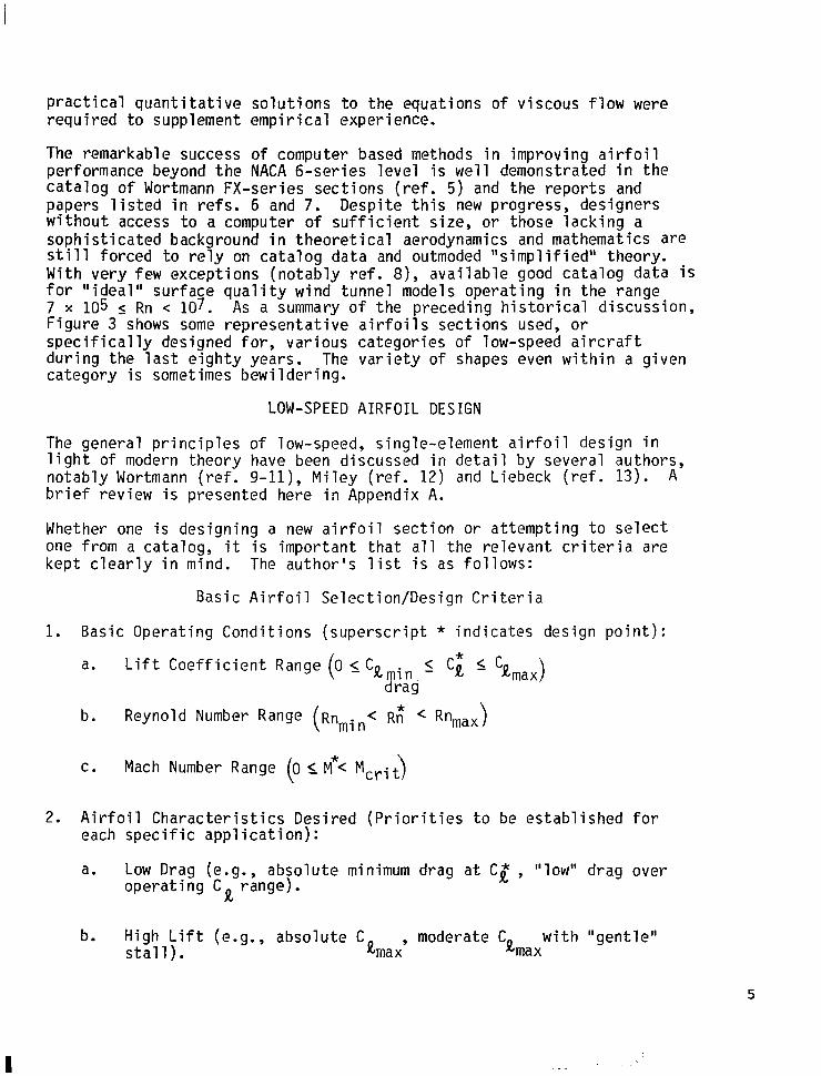
1. Basic Operating Conditions (superscript * indicates design point):

a. Lift Coefficient Range (0 <_ Cgmin <_ Ci I Cgmax) drag

b. Reynold Number Range ( Rnmin< Rt ( Rn,,, )

C. Mach Number Range ( 0 I M*< Merit)

2. Airfoil Characteristics Desired (Priorities to be established for each specific application):

a. Low Drag (e.g., absolute minimum drag at Cl , "low" drag over operating CR range).

b. High Lift (e.g., absolute CQ max'

moderate C stall). amax

with "gentle"

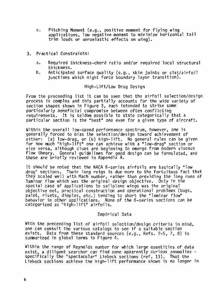
C. Pitching Moment (e.g., positive moment for flying wing applications, low negative moment to minimize horizontal tail trim loads or aeroelastic effects on wing).

3. Practical Constraints:

a. Required thickness-chord ratio and/or required local structural thickness.

b. Anticipated surface quality (e.g., skin joints or slat/airfoil junctions which might force boundary layer transition).

High-Lift/Low Drag Design

From the preceeding list it can be seen that the airfoil select ion/des process is complex and this partially accounts for the wide var iety of section shapes shown in Figure 3, each intended to strike some particularly beneficial compromise between often conf7icting requirements. It is seldom possible to state categorically that a

ign

particular section is the "best" one even for a given type of aircraft.

Within the overall low-speed performance spectrum, however, one is generally forced to bias the selection/design toward achievement of either: (a) low-drag, or (b) high-lift. No general rules can be given for how much "high-lift" one can achieve with a "low-drag" section or vice versa, although clues are beginning to emerge from modern viscous flow theory. General guidelines for good design can be formulated, and these are briefly reviewed in Appendix A.

It should be noted that the NACA 6-series airfoils are basically "low drag" sections. Their long reign is due more to the fortuitous fact that they scaled well with Mach number, rather than providing the long runs of laminar flow which was the original design objective. Only in the special case of applications to sailplane wings was the original objective met, practical construction and operational problems (bugs, paint, rivets, dimples, etc.) tending to abort the "laminar flow" behavior in other applications. None of the 6-series sections can be categorized as "high-lift" airfoils.

Empirical Data

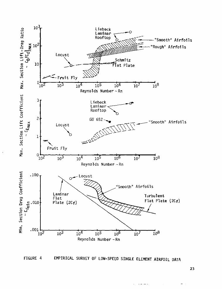
With the preceeding list of airfoil selection/design criteria in mind, one can consult the various catalogs to see if a suitable section exists. Data from these standard sources (e.g., Refs. 2-5, 7, 8) is summarized in global terms in Figure 4.

Within the range of Reynolds number for which laroe quantities of data exist, a dil specifically Liebeck sect

igent searcher can the "spectacular"

ions achieve the h i

find some apparently curious anomalies - Liebeck sections (ref. 13). That the gh-lift performance shown is no longer in

6

serious question, nor are the reasons such performance is achieved. What remains unclear is the nature of the trade-offs in section characteristics which are available between the "feasible upper bound" represented by the Liebeck sections and the "top-of-the-line" conventional sections within the shaded bands shown in Figure 4.

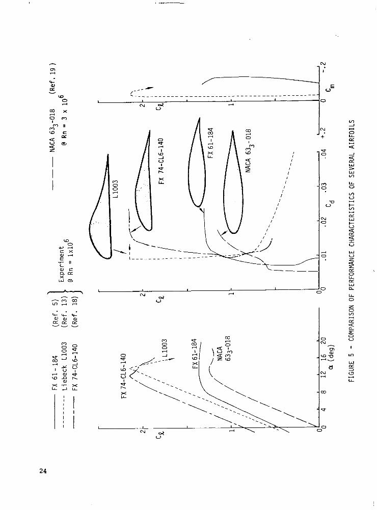
As a prerequisite to discussion of systematic methods for evaluation of these trade-offs, some appreciation of the parameters of boundary layer theory as they relate to airfoil performance is required. Figures 5 through 8 show some examples of the boundary layer characteristics of several familiar sections and the relationships between this data; and the more traditional display of global performance data, section geometry and pressure distributions is discussed in detail in Appendix B.

AIRFOIL SYNTHESIS

To advance beyond an empirically based approach to airfoil selection, or to consider the prospect of tailorinq airfoil sections to a specific application, it is necessary to understand the difference between a design approach based on "analysis" as contrasted with one based on "synthesis." The synthesis (inverse) approach to airfoil design begins with the boundary layer characteristics as they effect the pressure distribution and ultimately define and limit the performance of a section in every way. The airfoil shape is derived last in this process, and is that physically realizable contour which. provides the desired flow characteristics. Synthesis is almost the direct opposite to the traditional "empirical" (analysis) approach wherein one begins with a shape which yields a pressure distribution and a set of boundary layer characteristics, and thus initial values of lift, drag and moment. Performance requirements are finally met by trial and error modification of the shape. Whether these modifications are made to a wind tunnel or computer model, the basic process is one of iterative cut-and-try until the solution "converges."

AN INVERSE AIRFOIL DESIGN TECHNIQUE

While the possibility of synthesizing an airfoil has been recognized for many years, it has only been possible to implement satisfactory inverse methods (based on modern boundary layer theory) since the advent of the computer. Synthesis approaches have been employed by Wortmann (ref. 9) and more recently by Liebeck (ref. 13). A very general technique for airfoil synthesis (applicable to both single- and multi-element section components) has recently been developed by Henderson (ref. 14), based on proven integral boundary layer techniques described largely in Schlichting (ref. 15). While the specific techniques used in the overall program may s.eem.almost old fashioned, the program has proven to be very satisfactory in practice and is quite a powerful tool for both single and multi-element airfoil synthesis (particularly when coupled with the

7

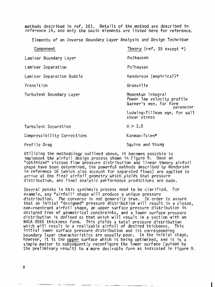
methods described in ref. 16). Details of the method are described in reference 14, and only the basic elements are listed here for reference.

Elements of an Inverse Boundary Layer Analysis and Design Technique

Component

Laminar Boundary Layer

Laminar Separation

Laminar Separation Bubble

Transition

Turbulent Boundary Layer

Theory (ref. 15 except *)

Polhausen

Polhausen

Henderson (empirical)*

Granville

Momentum integral Power law velocity profile Garner's eqn. for form

parameter Ludwieg-Tillman eqn. for wall shear stress

Turbulent Separation H > 3.0

Compressibility Corrections Karman-Tsien*

Profile Drag Squire and Young

Utilizing the methodology outlined above, it becomes possible to implement the airfoil design process shown in Figure 9. Once an "optimized" viscous flow pressure distribution and linear theory airfoil shape have been determined, the powerful methods described by Henderson in reference 16 (which also account for separated flows) are applied to arrive at the final airfoil geometry which yields that pressure distribution, and final analytic performance predictions are made.

Several points in this synthesis process need to be clarified. For example, any "airfoil" shape will produce a unique pressure distribution. The converse is not generally true. In order to assure that an initial "designed" pressure distribution will result in a closed, non-reentrant airfoil shape, an upper surface pressure distribution is designed free of geometrical constraints, and a lower surface pressure distribution is defined as that which will result in a section with an NACA OOXX thickness form. This yields a total pressure distribution which will result in a realizable airfoil of desired thickness. This initial lower surface pressure distribution and its corresponding boundary layer characteristics are usually poor. In the initial stage, however, it is the upper surface which is being optimized, and it is a simple matter to subsequently reconfigure the lower surface (guided by the preliminary result) to a more desirable form as indicated in Figure 9.

8

--~. -__--. .--... .-..-.._---.. _

The program allows a rather arbitrary specification of upper surface recovery region form parameter (H) variation as a primary input. Thus one can systematically study the effect of this important parameter easily and in some detail before proceeding to more detailed design calculations. This feature will be demonstrated shortly. The significance of various form parameter variations is discussed in Appendix B.

The most difficult parameter to specify correctly at the outset is the trailing edge pressure coefficient. This parameter has a very powerful effect on the design lift level a theoretical section will achieve, and to date the determination of its final "correct" value has generally required an iterative approach. by Liebeck (ref. 13).

The problem is discussed at some length

Probably the weakest part of the theoretical performance estimation procedure is calculation of profile drag. In principle, at the final stage in the design cycle one can integrate the total pressure and skin friction drag components and arrive at a total profile drag coefficient. Experience to date with viscous flow programs which accurately predict pressure distributions and hence lift and pitching moments gives generally less accurate drag estimates. This is due primarily to the fact that drag is usually two orders of magnitude lower than lift, and whereas errors in lift computations are small with a good pressure distribution predictor, errors in pressure integration (particularly in the leading edge region) tend to be on the same order as pressure drag values. Thus for simplicity, the present state of the art is to rely on the method of Squire and Young (ref. 15) for total drag prediction and, in the present case, a supplementary calculation of skin friction drag to provide a clarification of the magnitude of this component within the total drag value. This procedure has been found to be reasonably adequate, at least for purposes of comparing the drags of single-element sections. While absolute values of Squire and Young drag may sometimes be questionable, anyone experienced with the pecularities of two-dimensional wind tunnel testing (particularly at high-lift values) must realize the magnitude of the error band in "good" experimental drag data.

SOME RESULTS

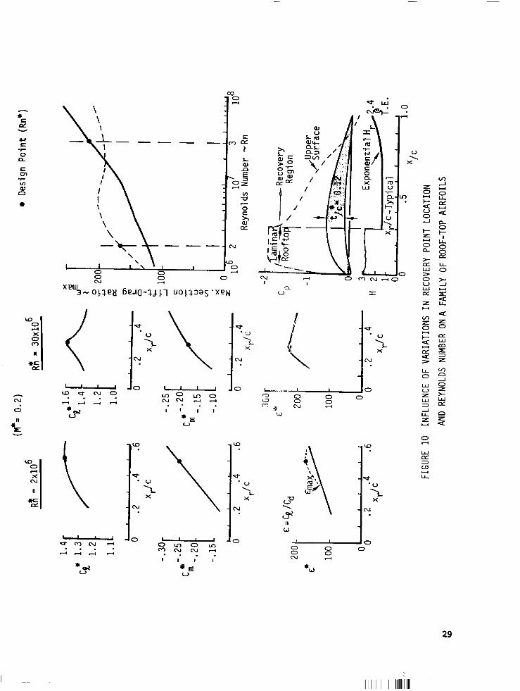
To indicate the use of the above methodology, two examples have been chosen to demonstrate several aspects of the influence of Reynolds number on airfoil characteristics. Figure 10 demonstrates the results obtainable from a parametric study of the influence of variations of recovery point location and Reynolds number on a family of sections with simple roof-top pressure distributions (cf. Fig. 9), and a common specified exponential form factor variation in the recovery region. The principal observations to be made in this example are the significant difference in "optimum" recovery point between sections designed (for

9

high lift-drag ratios) at two million and thirty million Reynolds number, and the ultimate desirability of designing to full-scale Reynolds number conditions (i.e., 30 x 106 in this case) to achieve maximum performance, despite the fact that such results may appear inferior to those obtained from a design optimized at wind tunnel conditions when both are tested at low Reynold numbers.

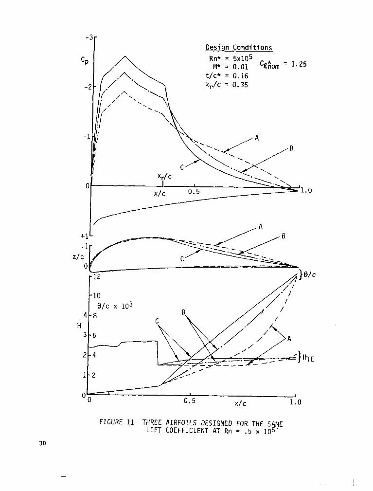
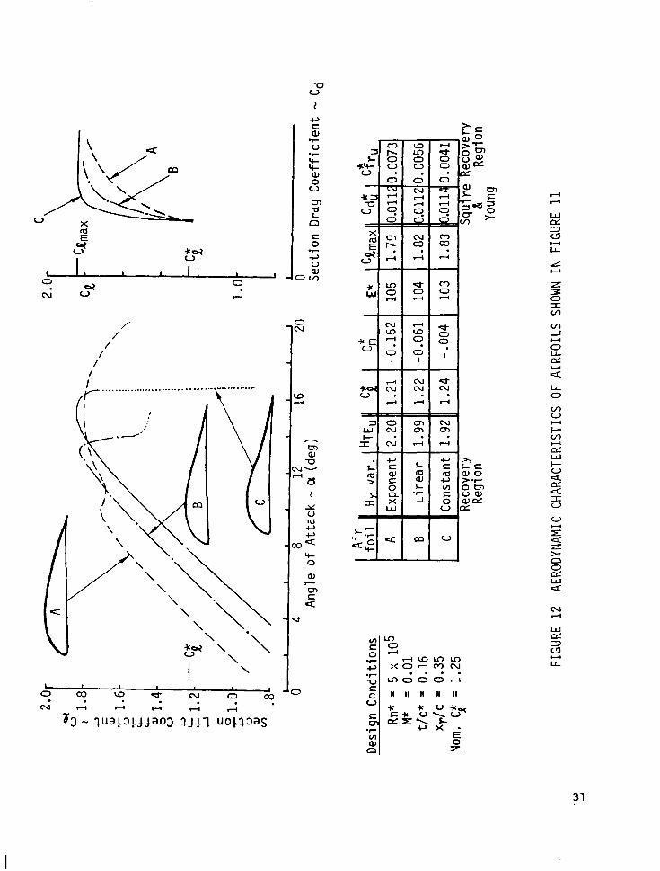
Figure 11 shows the effect of a systematic variation of recovery region form parameter on the shape and characteristics of three airfoils designed to the same lift coefficient level at a Reynolds number of five-hundred thousand. The performance characteristics of these sections are summarized in Figure 12, and clearly show the trades available in lift, drag, pitching moment and stall break from different specifications of recovery region characteristics.

The results shown in Figure 12 are generally nonobvious and are of some interest in view of the discussion in Appendix B and the fact that relatively little modern experimental data exists for sections designed specifically for this low value of Reynolds number. The stall behavior of the three sections can be understood on the basis of the discussion in Appendix B regarding the correlation between boundary layer form parameter (H) variation and upper surface separation progression.

A more subtle and remarkable aspect of the results shown in Figure 12 is that the net Squire-Young drag of all three sections at the design point lift coefficient is nearly the same. The rate at which the drag rises between the design point and maximum lift coefficients will be different, however, reflecting the way in which flow separation progresses on the three sections as stall is approached. The example calculations also show the relative values of upper surface recovery region (turbulent) skin friction coefficient relative to the total upper surface profile drag coefficient. Although the highly concave recovery pressure distribution of Airfoil C (which approaches a Stratford type recovery, c.f. Appendix B)shown in Figure 11 has the lowest skin friction coefficients, it also has the highest rate of growth (and final trailing edge value) of boundary layer momentum thickness. Thus while Airfoil C has the lowest skin friction drag it has the highest pressure drag and in the overall balance, all three sections exhibit similiar net profile drag values. This effect is not limited to the low Reynolds number case shown. As Reynolds number increases, the pressure drag becomes the increasingly dominant drag term, and minimization of the recovery region turbulent skin friction coefficient by employing a Stratford type recovery becomes increasingly less satisfactory.

CONCLUDING COMMENTS

A review of the history and present state of the art of low-speed single-element airfoil design has been presented, leading to a description of a powerful new inverse boundary layer scheme which can be used to synthesize an airfoil section tailored to the requirements of a

10

specific aircraft. The basic intent of this paper has been to provide background and motivation for this alternative approach to airfoil design, as contrasted with the more traditional "design by experiment/analysis" approach to the problem. Along the way (Appendix B) it has been possible to clarify the performance characteristics of sections of quite different geometry and design objectives, and indicate the influence of Reynolds number on both "low-drag" and "high-lift" sections. Several examples of parametric analyses using the "synthesis" methodology have been presented which only hint at the potential of these new techniques.

It has been shown that airfoil desi n (even when limited to very low Mach numbers and single-element sections 9 is a hugely complex problem to which no single "best" solution exists even for a single specialized category of aircraft type. On the other hand, it is clearly possible to derive a section biased and optimized to the taste of an individual aerodynamicist with a great deal more intelligence than was possible less than a decade ago. Much work still needs to be done, however, to finally free the hang glider designer from reliance on his present very slender catalog of airfoil candidates.

REFERENCES

1. McMasters, J. H. and Greer, R. R., "Large Winged Surface Effect Vehicles," in Jane's Surface Skimmers - Hydrodoils and Hovercraft, 1975-76, Ray McLeavy, ed. NY: Franklin Watts (for Janes Yearbook: London), 1975, pp. 425-33.

2. Abbott, I. H. and von Doenhoff, A. E., Airfoil Sections, NY: Dover, 1959.

3.

4.

Riegels, F. W., Airfoil Sections, London: Butterworth, 1961.

Jacobs, E. N. and Sherman, A., "Airfoil Section Characteristics as Affected by Variations of the Reynolds Number," NACA TR 586, 1937.

5. Althaus, D. StutQarter Profil Katalog I, Stuttgart University, 1972.

6. McMasters, J. H., "Low-Speed Airfoil Bibliography," Tech. Soaring, Vol. 3, No. 4, Fall 1974, pp. 40-42.

7. Hoerner, S. F. and Borst, H. V., Fluid-Dynamic Lift, Hoerner Fluid Dynamics, P.O. Box 342, Brick Town, N.J. 08123, 1975.

8. Schmitz, F. W., Aerodynamik des Flugmodells, Trans: N 70-39001, Nat. Tech. Info. Service, Springfield, Va., Nov. 1967.

11

9.

10.

11.

12.

13.

14.

15.

16.

17.

18.

19.

20.

Wortmann, F. X., "Experimental Investigations on New Laminar Profiles for Gliders and Helicopters," Ministry of Aviation Translation TIL/T.4906, March 1960 (Avail. ASTIA, Arlington, Va.) (I. Flugwiss, Vol. 5, No. 8, 1957, pp. 228-48).

Wortmann, F. X., "Progress in the Design of Low Drag Airfoils," in Boundary Layer and Flow Control, G. V. Lachmann, London, 1961, pp. /48-/O.

Wortmann, F. X., "A Critical Review of the Physical Aspects of Airfoil Design at Low Mach Number," in Motorless Flight Research - 1972, J. L. Nash-Weber, ed, NASA CR 2315, Nov. 1973.

Miley, S., "On the Design of Airfoils for Low Reynolds Numbers," AIAA Paper No. 74-1017, September 1974.

Liebeck, R. H., "Design of Subsonic Airfoils for High Lift," Journal of Aircraft, Vol. 15, No. 9, September 1978, pp. 547-61.

Henderson, M. L., "Inverse Boundary Layer Technique for Airfoil Design," Proceedings NASA Advanced Technology Airfoil Research (ATAR) Conference, March 1978.

Schlichting, H., Boundary Layer Theory, NY: McGraw-Hill, 1960.

Henderson, M. L.: Inverse Boundary Layer Technique for Airfoil Design. Advanced Technology Airfoil Research, Volume I, NASA CP-2045, Pt. 1, 1978, pp. 383-397.

McGhee, R. J. and Beasley, W. D., "Low Speed Aerodynamic Characteristics of a 17-Percent Thick Airfoil Section for General Aviation Applications," NASA TN D-7428, 1973.

Wortmann, F. X., "The Quest for High Lift," AIAA Paper No. 74-1018, September, 1974.

Loftin, L. K., Jr., and Bursnall, W. J., "The Effects of Variations in Reynolds Number Between 3.0x10‘ and 25.0~10~ Upon the Aerodynamic Characteristics of a Number of NACA 6-Series Airfoil Sections," NACA TR 964, 1946.

Stratford, B. S., "The Prediction of Separation of the Turbulent Boundary Layer," Jour. Fluid Mech., Vol. 5, January 1959, pp. 1-16.

APPENDIX A: BASIC AIRFOIL DESIGN

The purpose of this appendix is to provide a brief tutorial review of some of the principles of airfoil design. The discussion follows that of Wortmann (ref. ll), Miley (ref. 12) and Liebeck (ref. 13).

12

All practical airfoils will carry some lift loading (whether high, low, or moderate) at some desired operating condition, and this will be characterized by generation of some peak level of negative pressure coefficient on the upper surface of the section, followed by recovery to near free-stream conditions at the trailing edge. The pressure loading on the lower surface will depend on factors like required maximum section thickness, establishment of favorable pressure gradients for low-drag at the section design lift level, and the requirements of satisfactory "off-design" performance at low section lift coefficients. At some point on both surfaces of the contour, the initial run of laminar boundary layer flow will transition to turbulent flow, the particular transition points being strongly dependent on the Reynold number, the form of the pressure distribution (or the profile shape which generates it), the surface quality of the section, and the free-stream turbulence level. All other factors being equal, the natural transition point will move forward on the profile as Reynolds number increases.

At this point there is a parting of the ways as one seeks either high-lift, or low-drag performance at low-to-moderate lift coefficients. To achieve low-drag, the longest possible runs of laminar flow are desired on both surfaces of the section followed by an orderly transition to thin turbulent boundary layer flow as the pressure recovers to tramg edge conditions; and separation is to be avoided like the plague.

In the high-lift case, attention mainly focuses on the upper surface. As in the low-drag case laminar flow is sought, together with high negative pressures over the forward portion of the section. The problem in the high-lift case is not necessarily to delay the onset of turbulent flow, but rather to cause an orderly transition at some optimum point to a healthy thin turbulent boundary layer over the pressure recovery region to allow the flow to decelerate from the high peak values reached on the forward portion without significant separation. The "optimum" high-lift upper surface pressure distribution will thus be constructed to produce the highest possible loading on the forward portion of the profile, consistent with the recovery capability of the turbulent boundary layer beginning at an "optimum" transition point. At low Reynolds numbers, getting rid of laminar flow at the recovery point and avoidance of large scale laminar separation become a major consideration.

A major constraint on the high-lift section is the character of the stall break; all things being equal, a gradual stall progressing from the trailing edge is desired. It should also be noted that the bulk of "good" high-lift sections achieve their maximum lift coefficients after upper surface (trailing edge) separation has begun. Controlled laminar separation bubbles may even be tolerated if they lead to orderly transition to turbulent flow in the pressure recovery region and do not burst before trailing edge separation is well developed.

In the high-lift case, the lower surface pressure distribution will be tailored in much the same fashion as in the low-drag case, although the

13

lower surface pressure distribution can be made to produce a significant portion of the net lift and/or alter the pitching moment characteristics. This factor and the influence of various forms of upper surface distribution on section pitching moment coefficients are indicated in Figures 9 through 12 and in Appendix B.

APPENDIX B: SOME RELATIONSHIPS BETWEEN AIRFOIL

PERFORMANCE AND BOUNDARY LAYER CHARACTERISTICS

While most aerodynamicists have some appreciation of the section geometric parameters (e.g. thickness, camber, leading edge radius, trailing edge angle) which may influence performance, relatively few have a corresponding "feeling" for the fundamental parameters of boundary layer theory (e.g. form parameter, momentum thickness), and how these parameters are influenced by scale effects. The purpose of this appendix is to provide a brief evaluation of the boundary layer characteristics of several representative airfoils, and a description of how these parameters relate to the more familiar presentations of pressure distributions and global performance characteristics. An understanding of the connection between boundary layer behavior, pressure distribution, and section geometry as they influence performance is essential to success in the synthesis approach to design.

The performance characteristics of four familiar sections are shown in Figure 5. Two of these sections (the NACA 633-018 and Wortmann FX 61-184) have been designed primarily for low-drag, and the other two (the FX 74-CL6-140 and Liebeck L1003) for high-lift. These sections actually represent something of a continuum in that the NACA section is a classic "minimum drag" shape while the Liebeck is a pure "high-lift" section. The Wortmann FX 61-184 (ref. 5, 11) is a classic 1960 vintage sailplane section designed for "low-drag" over a "wide" range of lift coefficients, with a compromise struck between absolute low drag, thickness, and a very benevolent stall behavior at a moderate maximum lift coefficient.

The FX 74-CL6-140 (ref. 18) on the other hand, represents an attempt to design a section with the same level of maximum lift coefficient as the Liebeck, but with a biased compromise again being struck between thickness, maximum lift, wide "drag bucket" and satisfactory stall characteristics. All four sections are quite different in shape, and in the absence of detailed information on the types of pressure distribution and boundary layer characteristics (including an evaluation of the post-separated flow region) one is provided only superficial clues to why each of these sections exhibits such different performance characteristics.

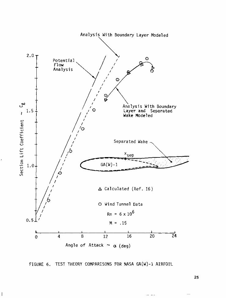
As an aside, the influence of flow separation on the performance of a section and the importance of accurately modeling this effect in a theoretical design exercise have been graphically demonstrated by Henderson (ref. 16). Figure 6 shows an experimental lift curve for the NASA GA(W)-1 section (ref. 17) in comparison with theoretical

14

Calculations made with increasingly sophisticated analytical techniques. For this particular section, Figure 6 shows that modeling the attached boundary layer flow remains inadequate in predicting the variafix lift with angle of attack beyond 75% of the final maximum lift coefficient value. The full theory developed by Henderson (ref. 16), which models both the boundary layer and separation, provides excellent predictions however. This improved methodology (which extends to multielement sections) represents a major, and so far unique, advance in computational capability.

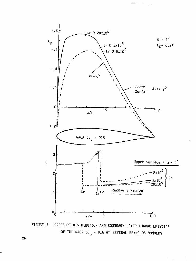
TO better understand the differences in performance and shape between the sections shown in Figure 5, it is necessary to evaluate in detail the pressure distributions and boundary layer parameter (specifically the form parameter, H) variations for each section. Example data for the NACA 633-018 (ref. 19) at 2O angle of attack (within the drag bucket of the section) are shown in Figure 7 for three widely different Reynolds numbers. The classic 6-series aft-end shape corresponds to a roughly linear rise in the recovery region pressure distribution, and consequent form parameter (H) variation shown. The influence of Reynolds number on the location of the point of natural transition is indicated, and clearly shows the difficulty of achieving long runs of laminar flow as Reynolds number increases.

As shown in Figure 11, the shape and magnitude of the form parameter (the ' ratio of boundary layer displacement thickness to momentum thickness)

variation in the pressure recovery region of the airfoil correlate in general with the shape of the pressure distribution in this region. The specification of recovery region form parameter variation is one of the central inputs in the Henderson inverse method described previously. AS discussed in Schlichting (ref. 15), laminar separation occurs when H reaches 3.5 and turbulent separation begins when H exceeds about 3.0. The influence of the H-factor variation on airfoil stall behavior will be discussed presently.

Wortmann (refs. 9-11) has argued that there are advantages to a "concave" recovery pressure distribution (with near constant value of recovery region form parameter) for drag reduction, compared to the linear or convex pressure distributions associated with earlier profiles, including many of the G'ottingen/Joukowski airfoils (c.f. Figure 3). The basic principles of the design of Wortmann's sailplane and related sections (including the FX 61-184) with concave pressure rises have been thoroughly discussed in references 9 through 11, and by Miley (ref. 12). These references also discuss the importance of properly contouring both the upper and lower surfaces of low-drag profiles.

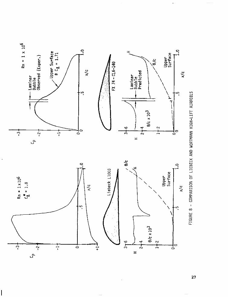
Turning attention to the high-lift airfoils cases, it is interesting to compare the pressure distributions and boundary layer characteristics of the Wortmann FX 74-CL4-140 (ref. 18) and Liebeck L1003 (ref. 13) shown in Figure 8, and contrast this data with that for the NACA 633-018 in Figure 7.

15

The Liebeck sections are of great theoretical interest for several reasons. Members of the family apparently approach the upper limit of lift coefficient achievable with a single-element section without mechanical boundary layer control. The sections also exhibit commendably low drag coefficients in the region of the design lift coefficient and low pitching moments. In exchange for these desirable characteristics, the stall behavior is wretched and the undersurface separates at rather high (positive) lift coefficients, thus limiting "high-speed" performance. This latter factor can be partially ameliorated by use of a camber changing trailing edge flap; however, the abrupt stall behavior is a fundamental characteristic of the basic family.

The Liebeck sections have been theoretically designed by the previously described synthesis process, in this case by use of a Stratford recovery region pressure distribution (ref. 20) to establish the maximum level of negative pressure on the upper surface "roof top" region of the section. The Stratford recovery region pressure distribution is that which, for a turbulent flow, results in a boundary layer which is everywhere equally close to separation. Thus, to within the accuracy of the Stratford formulation, the recovery region boundary layer is either completely attached or completely separated - there is no (theoretical) middle ground. This factor accounts for the very abrupt stall behavior of the sections. Thus, by reliance on the Stratford distribution, Liebeck generated the single class of high lift sections which can be "optimized" and analyzed without recourse to explicit partially separated flow calculations. Herein lies the success Liebeck had in designing to very much higher lift coefficients and section lift-drag ratios than had once been thought possible for a single-element section. The resulting shapes and pressure distributions for Liebeck sections are entirely non-obvious and the prospects of happening on them by "cut-and-try" were remote. This example provides a strong motivation for use of inverse methods.

The experimental verification of the predicted performance of the Liebeck sections, and by extension the validation of the Stratford theory, apparently opens a whole new prospect in high-lift airfoil design. However, the inability of Liebeck's methodology to account for partially separated flows, and the resulting formal reliance on the Stratford distribution, severely circumscribe the range of sections which can be designed. The possible trade-offs in performance between the Liebeck sections and the range of conventional sections shown in Figure 4 remain obscure.

The result of a highly sophisticated attempt to design such an "intermediate" airfoil, which trades some drag and thickness for a better stall behavior, while acheiving the same high-lift level, is represented by the Wortmann FX 74-CL(X)-140 pair discussed in ref. 18. Referring to Figure 8, one sees that the Liebeck and Wortmann pressure distributions are quite different, although both have "concave" distributions in the recovery region. Where Liebeck uses a well defined "instability" region as described by Miley (ref. 12) to achieve orderly transition to

16

turbulent flow in the recovery region, Wortmann forces the formation of a "well-behaved" thin laminar separation bubble which acts as a passive boundary layer trip.

Reviewing the performance curves for the Wortmann and Liebeck high-lift sections shown in Figure 5, one sees the consequences of the two approaches to the design problem. Looking at the resulting airfoil shapes and pressure distributions in Figure 8, one sees little in common between the two sections however. To see how "equally" high-lift coefficients are generated by two such dissimilar sections, one must refer to the details of the boundary layer characteristics for the two airfoils.

For both the Liebeck and Wortmann sections, recovery begins at about 40% of the chord aft of the leading edge. Prior to this, the "laminar H" for the Liebeck section is nearly constant through the instability region, falling abruptly to an initial "turbulent" value as the flow transitions. By contrast, on the Wortmann section the laminar H rises abruptly prior to transition until a value of H for laminar separation is reached, following which a "short bubble" is formed leading to transition and turbulent reattachment at the beginning of the recovery region.

Once into the recovery region, the turbulent form parameters on the Liebeck section rise rapidly to an initially high value and then begin a further very gradual linear rise to a point just short of the trailing edge. This recovery region form parameter variation is characteristic of a Stratford imposed pressure distribution.

On the Wortmann section, the turbulent form parameter does not jump initially, but rises instead from its starting value behind the laminar bubble at a nearly identical rate to that of the Liebeck/Stratford, until it hooks upward at the end. The result is again a generally concave pressure distribution on the recovery portion of the Wortmann section.

Comparison of these form parameter variations for two very different "looking" sections clarifies much of the difference in stall behavior between the sections. On the Liebeck section, as angle of attack is increased beyond the "design" value (design lift coefficient equal to 1.8), the recovery region form parameter level is shifted progressively upward until a value of approximately 3.0 is reached, at which point turbulent separation begins. With the Liebeck/Stratford recovery pressure distribution, the form parameter level is almost constant across the bulk of the recovery region. Thus, if nothing else (a laminar short bubble for example) interferes, the whole recovery region becomes "critical" with respect to separation at nearly the same time, and an abrupt stall subsequently occurs. By contrast, the recovery region form parameter on the Wortmann section does not reach so uniform a critical level as angle of attack is increased towards stall. This is reflected in the more gradual stall break for the Wortmann section. The existence of the short bubble ahead of the recovery point on the Wortmann section

17

IllI -Ill I I1 II I lllllllllIllllIIlllII I II llIlllIIllllllllll I llllllllllllllllIlI

throughout this approach to stall clouds the issue of how the stall progresses, and the critic will note that the stall behavior is not that much better than the Liebeck. That the stall progresses non-catastrophically (at least initially) from the trailing edge is indicated (c.f. Fig. 5) by the creeping drag rise as stall is approached and entered.

The preceeding examples are intended to be illustrative of a few well known sections and demonstrate some specific trends. The results shown are not necessarily typical of wide classes of sections and the possible ranges of form parameter variation and pressure distribution are enormous. These limited examples do, however, demonstrate the level of detailed analysis which modern theory can provide, and the necessity of delving this deeply into detail in order to understand differences and similarities between airfoils with different shapes and global performance characteristics, and finally to design an optimized profile for a given application. Obviously, much more could and should be said on these topics. In addition, much needs to be said regarding the problems of "optimizing" both upper and lower surface contours, and the influence on drag of form parameter variation, boundary layer momentum thickness, transition point, etc. All of these investigations require a technique by which the important variables of the problem can be varied in an orderly and systematic fashion, particularly as a function of Reynolds number. Such a technique has been described in this paper.

18

50

Spee

d-

V(m

/s)

10

100

Spee

d -

V(m

/s) 10

1

lo5

lob

Aver

age

Rey

nold

s N

umbe

r -

\n

= $-

10

Aver

age

Win

g C

hord

-

e (m

l

-Bird

s I

I 9

? *

.l .

10

10‘

10J

lor

1 10

1U

U

Win

g Lo

adin

g -

W/S

(N/m

2)

Win

g Sp

an

- b(

m)

FIG

UR

E 1

A G

UID

E TO

TH

E R

EGIO

NS

OF

LOW

-SPE

ED FL

IGH

T AT

STA

ND

ARD

SEA

LEVE

L C

ON

DIT

ION

S

.ch

Num

ber-M

rcra

ft

(Joukowski Airfoils)

1920 - 1940 ------- I I NACA '

' NACA 4-digit 7 - - 5-digit - - -- J

,-Boundary Layer

---A --

I I I Liebeck I l----l

Low Mach High Mach (< 1)

--- t

Wortmann

Eppler

------ --

1960 - Present Computational Aerodynamics

NASA GA ( ) I I

FIGURE 2 SINGLE ELEMENT AIRFOIL EVOLUTION

20

'Pearcey

Garabedian' Korn

Whitcomb

- --

. . ..-- . . . . m-.-m.. . ..- __. ..__. . . ..- .-.. _.--

,--Equivalent "Airfoil" Envelope

Crane Fly (c = .004 m)

Pigeon (c = .10 m)

NACA 6409

Eppler -387

Benedek 6356 b

Jedelsky EJ-75

FIGURE 3a SOME VERY LOW-SPEED AIRFOILS

21

/I iiiiiii i I i iillilltilll

HAN

G G

LID

ERS

Lilie

ntha

l

HU

mN

PO

WER

ED AI

RC

RAF

T

G'd

535

SAIL

PLAN

ES

GEN

ERAL

AVI

ATIO

N

NAC

A 24

12

Cul

ver/J

ense

n

Love

joy

67O

r.15

FX 7

2-15

08

FX 6

7-K-

150

1'.

FX 7

6-G

A-20

/170

Ki

cenl

uk

TK73

15

FX 7

6-M

P-18

0 Li

ebec

k L1

003M

Hig

h PR

Rog

allo

Li

ssam

anlM

acC

read

y Ep

pler

E6

03

.-r

1L

!?FP

RES

ENTA

TIVE

LO

W-S

PEED

AIR

FOIL

SE

CTI

ON

S

103,

102. -

Locust

lo,- )&-

~~~ Fruit Fly

"Smooth" Airfoils

"Rough" Airfoils

1 1% 103 lo4 105 106 107

I lo8

Reynolds Number-Rn

3- Liebeck Laminar Rooftop

l--

-\ Fruit Fly

402 103 10T 105 106 Reynolds Number -Rn

"Smooth" Airfoils

Turbulent Flat Plate

Reynolds Number -Rn

(2Cf)

FIGURE 4 EMPIRICAL SURVEY OF LOW-SPEED SINGLE ELEMENT AIRFOIL DATA

23

-

FX 6

1-18

4 ---

-----

Lieb

eck

L100

3 Pm

- FX

74-

CL6

-140

(Ref

. 5)

I

---

NAC

A 63

3-01

8 (R

ef.

19 )

(Ref

. 13

) Ex

perim

ent

@ R

n =

3 x

lo6

(Ref

. 18

) 8

Rn

= 1~

10~

I FX

74-

CL6

-140

/y:\

2-

/ ' I

/ \

/ \

/ :

'

I

I I' /

: L1

003

/ \

I 1

/'

12

16

20

Q (

deg)

r 1

L100

3

--+

I /--

---

I I \

I I I I /

(@--I

L

!I

FX 7

4-C

L6-1

40

C

, 1

FX 6

1-18

4

NAC

A 63

3-01

8

FIG

UR

E 5

- C

OM

PAR

ISO

N O

F PE

RFO

RM

ANC

E CH

ARAC

TER

ISTI

CS

OF

SEVE

RAL

AIR

FOIL

S

Analysis With Boundary Layer Modeled

Wake Modeled

I /

I Separated Wake

/

/ /

d

/

/ /

/

/ I Q Calculated (Ref. 16)

0 Wind Tunnel Data

Rn = 6 x106

M = .15 , , , , , 0 4 8 12 16 20 24

Angle of Attack w a (deg) FIGURE 6. TEST THEORY COMPARISONS FOR NASA GA(W)-1 AIRFOIL

25

-. 8

Upper oa Surface

a = 2'

cg' 0.25

‘: s

H

2

1

0

I

tr ,

Upper Surface 8 a= 2'

I I I* M--8~10~ I M-c I de4 Rn -_---- -c -33x106 }

_____----- -w-- ---20x106 I tr Recovery Region

+

I I 1 I 1 1 1

x/c .5 1.0

FIGURE 7 - PRESSURE DISTRIBUTION AND BOUNDARY LAYER CHARACTERISTICS

OF THE NACA 633 - 018 AT SEVERAL REYNOLDS NUMBERS

26

Rn

= 1x

106

-3

C;=

1.

8

cP

-2

-1

Rn

= 1

x 10

6 -

- La

min

ar

Obs

erve

d (E

xper

.)

FX 7

4-

CL6

-140

I

.5

i.0

x/c

/ *I.

/H

I

/ /

/ U

pper

/

Surfa

ce

I I

I .5

1.

0 x/

c

----

-/ U

pper

Su

rface

I .5

1.0

x/c

FIG

UR

E 8

- C

OM

PAR

ISO

N OF

LIEB

ECK

AND

WO

RTM

ANN

HIG

H-L

IFT

AIR

FOIL

S

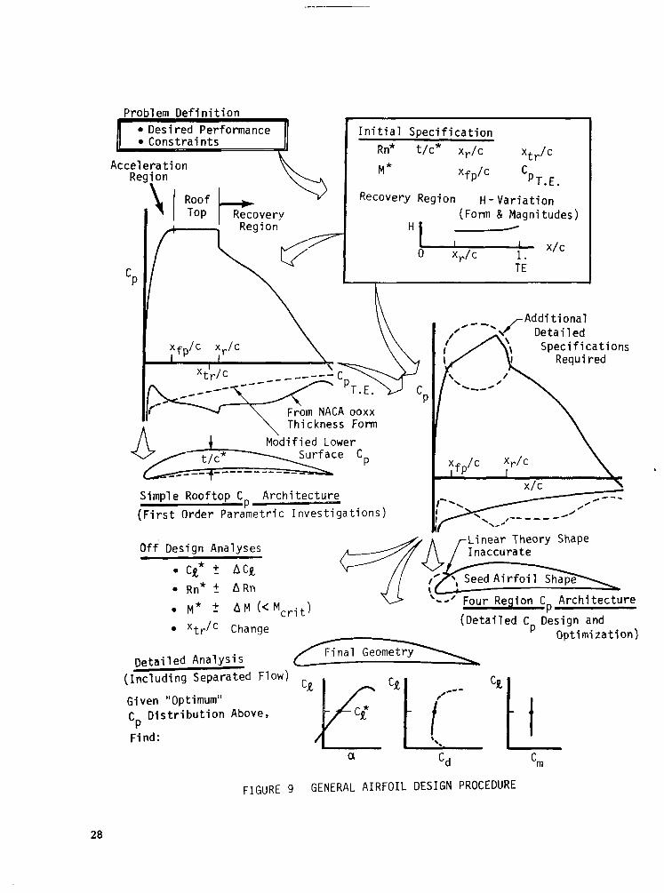
Problem Definition l Desired Performance Initial Specification

Rn* t/c* X,/C 'tJc Mf Xfp/c C

PT.E. Recovery Region H-Variation

(Form & Magnitudes)

"Iti x/c 0 x,/c 1.

TE

Additional Detailed

Specifications Required

From NACA ooxx Thickness Form

1 :fp/c :r’c \ Simple Rooftop Cp Architecture

(First Order Parametric Investigations)

Off Design Analyses

l cg* t ACCQ

l Rn *+ ARn

. M* 2 AM (<Merit)

l Xtrjc Change

nmtailed Analvsis

Four Region Cp Architecture

(Detailed Cp Design and n..+;m;T=+:rM\

YbVW. .-

(Including Separated Flow)

Given "Optimum" C, Distribution Above,

F?nd:

a 'd 'rn

FIGURE 9 GENERAL AIRFOIL DESIGN PROCEDURE

28

(m*=

0.2

)

RI);

= 2

~10~

R

*n =

30~

10~

l D

esig

n Po

int

(Rn*

)

+ :::

cQ

1.2

1.1 0.

2 .6

x

c r/

-.30

5lF

-.25

-.20

-.15

j, /,

0 .2

.4

.6

x,

/c

200

- E=

c9y/

C(j

E* 10

0 1 Y

Ok-

‘---

-2 vi4

.6

FIG

UR

E 10

ci$f

A

1.2

1.0

i 0 .2

xpa4

-.25

'm*

-.20

-.15

-.lO

0 .4

x,

/c

100 0 L-

0

.2

.4

x,/c

v,

I I

i O

lo6

; ’

’ ”

““,

’ ’

’ ’ “

“I 3

Rey

nold

s 'tk

mbe

r -R

n lo

8

INFL

UEN

CE O

F VA

RIA

TIO

NS I

N R

ECO

VER

Y POIN

T LO

CAT

ION

AND

REY

NO

LDS N

UM

BER

ON

A F

AMIL

Y O

F R

OO

F-TO

P AI

RFO

ILS

-3

P

-2 1

Design Conditions

Rn* = 5x105 M* = 0.01 cfiOm = 1.25

t/c* = 0.16 x,/c = 0.35

H

I I 0.5 x/c 1.0

FIGURE 11 THREE AIRFOILS DESIGNED FOR THE SAME LIFT COEFFICIENT AT Rn = .5 x 106'

30

I I

I I

I I

I I

1 I

0 4

8 12

I

16

Ang

le

of

Atta

ck

w a

(d

eg)

20

Des

ign

Con

ditio

ns

Rn*

=

5 x

105

Mf

= 0.

01

t/c*

= 0.

16

xr/c

=

0.35

N

om.

C;

= 1.

25 FIG

UR

E 12

I Ai

r I

, foi

l H

r va

r. H

TEu

'i C

i E"

'a

ma)

A

Exp

onen

t 2.

20

1.21

-0

.152

10

5 1.

79

ll0.0

11~0

.007

31

p c!

! cd

; !

Cbu

,

C

x /+

- .

i

/

+ l /

/ A

B

J 0 Sect

ion

Dra

g C

oeffi

cien

t e

Cd

6 Li

near

1.

99

1.22

-0

.061

10

4 1.

82

3.01

12 0

.005

6

C

Con

stan

t 1.

92

1.24

-.0

04

103

1.83

0.

0114

0.0

041

Rec

over

y S

auire

R

ecov

e R

egio

n-

'&

You

ng

Reg

ion

AER

OD

YNAM

IC CH

ARAC

TER

ISTI

CS

OF

AIR

FOIL

S SH

OW

N IN

FI

GU

RE

11