1

Low-Resolution Fault Localization Using PhasorMeasurement Units with Community Detection

Mahdi Jamei∗, Anna Scaglione∗, Sean Peisert†∗Arizona State University, {mjamei, ascaglio}@asu.edu

†Lawrence Berkeley National Laboratory, sppeisert@lbl.com

Abstract—A significant portion of the literature on fault local-ization assumes (more or less explicitly) that there are sufficientreliable measurements to guarantee that the system is observable.While several heuristics exist to break the observability barrier,they mostly rely on recognizing spatio-temporal patterns, withoutgiving insights on how the performance are tied with the systemfeatures and the sensor deployment. In this paper, we try to fillthis gap and investigate the limitations and performance limits offault localization using Phasor Measurement Units (PMUs), in thelow measurements regime, i.e., when the system is unobservablewith the measurements available. Our main contribution is toshow how one can leverage the scarce measurements to localizedifferent type of distribution line faults (three-phase, single-phaseto ground, ...) at the level of sub-graph, rather than with theresolution of a line. We show that the resolution we obtain isstrongly tied with the graph clustering notion in network science.

Index Terms—Fault Location, Distribution Grid, Identification,Community Detection.

I. INTRODUCTION

Phasor Measurement Units’ (PMU) data have the ability toprovide much more accurate event detection capabilities, evenwith relatively few measurements. Ardekanian et al., [1], forexample, use PMU data to detect and localize a change in theadmittance matrix of a distribution network. Zhou et al., [2]empoly PMUs to detect events in the distribution grid whenonly partial information is available. Our previous work [3]proposes a hierarchical architecture for event detection indistribution system using PMU data when only very fewsensors are available. Except for Ardekanian et al’s work [1],the literature on event detection is often in a low measurementsregime, that arises when the number of measurements is verysmall compared to system size, so the system is unobservable.

Event detection is, however, insufficient in most cases. Thelocalization of a line fault is a classic problem in powersystems management. In fact, it is an essential part of anyevent detection scheme, since the operators need to locate thefaulty section for isolation and service restoration. What werefer to as line fault is the short-circuit of a single-phase, twophase, or three-phase of a line with each other and/or withground with or without a fault resistance. As a result, a largemagnitude of fault current is withdrawn from the sources toprovide current for the short-circuited location.

This research was supported in part by the Director, Cybersecurity, En-ergy Security, and Emergency Response, Cybersecurity for Energy DeliverySystems program, of the U.S. Department of Energy, under contract DE-AC02-05CH11231 and de-oe0000780. Any opinions, findings, conclusions,or recommendations expressed in this material are those of the authors anddo not necessarily reflect those of the sponsors of this work.

Both for transmission and distribution grids, fault detectionand localization, particularly using PMU data, is still a veryactive area of research, which focuses more broadly on under-standing the root cause of abnormal changes recorded in thePMU measurements. Most of the work in the low measurementregime is in the distribution section of the grid. For example,Zhu et al., [4] propose an automated fault localization anddiagnosis for radial networks: specifically, using measurementsfrom the substation, the algorithm first finds a set of plausiblefault locations and then run a diagnosis to rank the differentpossibilities. Min and Santoso [5] propose a technique toremove the DC offset in the phasor data and improve thealgorithm intended to locate a momentary fault. Lee [6]uses synchronized voltage phasor measurements to search fora fault in a radial network in a timely manner. Dzafic etal., [7] propose a graph marking approach to spot the locationof a fault. There are a number of non-parametric methodsthat exploit spatio-temporal patterns, as well. Specifically, Jianet al., [8] extract the time-frequency signatures of voltageand frequency from a dictionary using matching pursuit [9],followed with a clustering algorithm for fault detection. Usingwavelet analysis on the voltage waveform generated duringa fault-induced transients, Borghetti et al., [10] obtain thelocation of a fault in the distribution network. While theexploitation of temporal patterns helps in the localization, theydo not provide an understanding on how the performance isaffected by the grid parameters and the sensor deployment.

Contribution: To dig deeper in the low measurement regime,in this work we do not look at temporal features (which canalways be incorporated in the algorithm) and take inspirationfrom Brahma’s work [11] to construct our models. Brahmaproposes a method using the bus impedance matrix of thesystems and pre/post fault voltage and current measurementsto pinpoint the location of a fault. The contribution of thispaper comes from unveiling the specific structure of the errorsthat localization algorithm based on PMU data tend to make,showing the fact that the errors swap nodes within very specificsub-graphs of the original grid topology. We can considerthese sub-graphs as communities, in which nodes are clusteredand show that community level fault localization is possible,even when the measurements are too few to have an accurateanswer. To the best of our knowledge, the connection betweenthe resolution of fault localization in power systems andgraph clustering is new. However, we acknowledge the graphclustering work in the transmission grid (see e.g., [12], [13]),in a different context (not for fault localization).

arX

iv:1

809.

0401

4v1

[cs

.SY

] 2

0 A

ug 2

018

2

II. SINGLE FAULT LOCALIZATION

Since distribution lines are untransposed, and because of theexistence of single phase and two phase laterals, we prefer touse a formulation that explicitly includes the phase-domain(and not the sequence-domain) voltage and current. For anetwork of size N the nodal voltages and injection currentsvectors are denoted by:

V =[V1, V2, . . . , VN

]T, I =

[I1, I2, . . . , IN

]Twhere depending on the number of phases connected to nodei, Vi and Ii can be row vectors of size 1, 2 or 3; the resultingV and I are M × 1. It is well-known that the nodal voltagesand injection currents satisfy Ohm’s law:

V = ZI, (1)

In (1), all the sources are modeled with their Norton equivalentand therefore their internal impedance is also included in thebus impedance matrix Z. Suppose a fault occurs at bus j andlet V0 and I0 denote the pre-fault and VF and IF denote thepost-fault nodal voltages and currents. Using (1) the followingtwo relationships hold:

V0 = ZI0, VF = Z(IF + IE) (2)

where IE is a sparse vector with non-zero elements at locationscorresponding to faulty phases of bus j, modeling the currentinjected by the fault at bus j (negative of the withdrawncurrent). Subtracting the pre-fault from the post-fault voltages:

VF −V0︸ ︷︷ ︸δV

= Z(IF − I0︸ ︷︷ ︸δI

+IE) (3)

Let K denote the total number of phases that are monitoredby the PMUs in the grid. For example, if we have two PMUs,where one is connected to a three phase node and the other isconnected to a single phase node, K = 3 + 1 = 4. Let:

Π =(ΠT

a | ΠTu

)T ∈ {0, 1}M×M (4)

that parses the voltage and current measurements into availableand unavailable measurements, where Πa ∈ {0, 1}K×M picksthe available measurements and Πu ∈ {0, 1}(M−K)×M selectsthe unavailable ones. Pre-multiplying both sides of (3) byΠa and also replacing Z in the first term with ZΠ−1Π andrearranging some terms, one can write:

δVa︷ ︸︸ ︷ΠaδV =

Za︷ ︸︸ ︷(ΠaZΠ−1

)(Π δI + Π IE)

δVa =(Zaa | Zau

)(ΠaδIΠuδI

)+ ZaIE

=(Zaa | Zau

)(δIaδIu

)+ ZaIE

= ZaaδIa + ZauδIu + ZaIE

(5)

where Zaa and Zau are the blocks of impedance matrixconnecting nodes with available data to the available andunavailable ones, respectively. Also, IE is the reordered vectorIE with indices corresponding to the nodes with available datain the top part and the rest at the bottom part.

Brahma [11] proposes the formulation above, assuming thatthe available measurements come from the sensors placedat the head of the substation and next to each distributedgenerator. Then, assuming that the term ZauδIu in (5) is small,the location of the faulty bus in his work can be found bysolving the following least-square problem [11]:

`∗ = argmin`∈F(t)

||δVa − ZaaδIa − ZaIE,`||22 (6)

where F(t) is the union of candidate fault locations subsets forfault type t. IE,` is a vector whose non zero entries correspondto a certain fault location ` and IG is a vector containing non-zero entries of IE,`. Note that in (6), the entries of IG arenot directly measured. To address this problem, Brahma [11]proposes to approximate the vector IG by adding up thecurrent injected by each source to the grid corresponding tothe faulty phases1 and subtracting the current that sources havebeen providing for the loads in the pre-fault condition. Thisputs a requirement on the µPMU placement strategy since eachsource requires a µPMU, to which it is connected.

Before going through further discussions about the per-formance analysis of single fault localization, we proposethe following modification to the method in (6). In orderto make the term ZauδIu as small as possible, the constantimpedance loads, constant power loads, and capacitors/reactorsare also included in the Z matrix. This modeling is accurate forconstant impedance loads. However, for constant power loadstheir equivalent impedance at the nominal voltage is includedin the bus impedance matrix, and the deviation of the actualconsumed power from the nominal is included in the nodalinjection vector. This modeling implies that the vectors IFand I0 are small and, accordingly, δIu is small as well. Fromnow on, we assume that this modification is included in themethod when we refer to (6).

III. FAULT LOCALIZATION PERFOMEANCE ANALYSIS

As stated before, the method in 6 is plagued by ambiguitiesin locating the fault precisely when K �M . The first sourceof ambiguity comes from the fact that the vector IG is anapproximation of the fault current. Therefore, a fault mightbe mis-located if the approximated fault current is close tothe actual fault current if there was a fault at the mis-locatedbus. The other source of ambiguity appears if the columns inthe Za for two locations are very similar; in fact, Za is a fatmatrix, so it is inevitable that columns will be correlated.

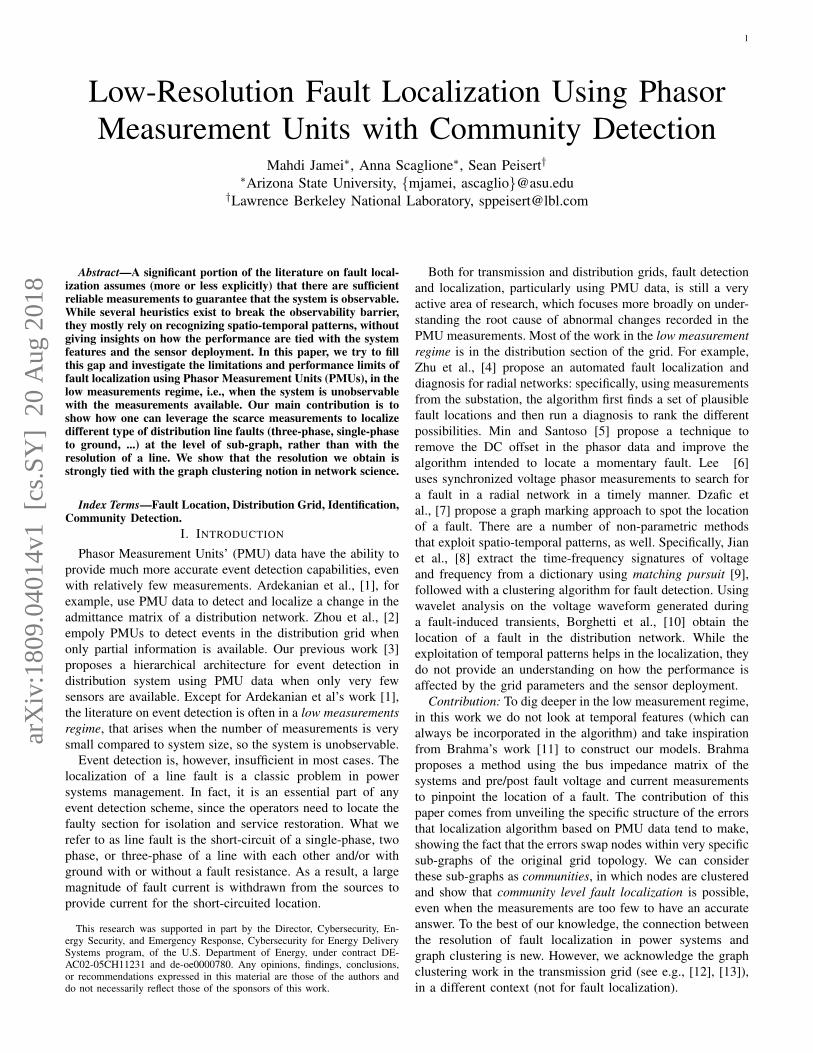
To illustrate why the latter occurs, consider the one-linediagram given in Fig. 1, where bus 1 is assumed to be thesource bus and is modeled with the Norton equivalent.2 The

1 2 3

4

12z 23z

0z 24z

Fig. 1. One-Line Diagram of an Example Radial Network

1The vector IG is of size 1, 2 or 3 depending on how many phases areimpacted by the fault.

2The network is modeled with its positive sequence impedance values inthis example for simplicity of illustration.

3

bus impedance matrix of this network is given below, wherethe columns are ordered based on the bus numbers.

Z =

z0 z0 z0 z0z0 z0 + z12 z0 + z12 z0 + z12z0 z0 + z12 z0 + z12 + z23 z0 + z12z0 z0 + z12 z0 + z12 z0 + z12 + z24

(7)

Now assume that we have sensors at bus 1 and 2, so that:

Za =

(z0 z0 z0 z0z0 z0 + z12 z0 + z12 z0 + z12

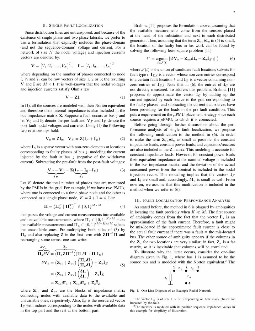
)and assume that we have access to the exact value of thefault current. Based on the given criterion for fault detectionin (6), the norm in the objective function would be the sameif the fault happened at bus 2, 3 or 4, since the columns areexactly the same. This situation can actually happen in radialgrids, if one looks at the way the bus impedance matrix isconstructed. To provide some intuition, consider a radial gridwith a single source and negligible line shunt components.Since there is no loop, the bus impedance matrix can beconstructed starting from the source bus and adding newnodes. When a new node j is added to an existing node i, thecolumn and row corresponding to the existing node is copiedon the column and row corresponding to the new node and theentry [Z]jj = [Z]ii + zadded line. Thus, the entries of column iand j are very similar. This process is sketched below, whena new node (Node 3) is added to the existing node (Node 2).

1 2 312z 23z

0z

1 212z

0z

Z =

(z0 z0z0 z0 + z12

)→Z =

z0 z0 z0z0 z0 + z12 z0 + z12z0 z0 + z12 z0 + z12 + z23

In fact, even if the columns are not exactly the same, they arevery similar and therefore correlated. Hence, an estimationerror can easily occur, due to the noise in measurementsor poor approximation of the fault current, and lead to theselection of an incorrect location. An example of this is whenthere are sensors at buses 2 and 3, and the impedance of line2-3 is small.

Za =

(z0 z0 + z12 z0 + z12 z0 + z12z0 z0 + z12 z0 + z12 + z23 z0 + z12

)In this case, distinguishing a fault between buses 2, 3 and 4would not be easy. This observation conforms to the topo-logical proximity of the nodes in a radial network, whereneighboring nodes tend to contribute to similar columns inthe bus impedance matrix.

A. Communities of Neighboring Nodes

The discussion above indicates that the errors that algorithmtends to make are swaps of nodes within very specific sub-graphs of the original grid topology, which have associatedcolumns in the bus impedance matrix that are very similar. Wecall these sub-graphs, communities. Clearly, these communities

are also dependent on the location of the sensors. Beforedigging into this phenomenon further, we notice the termZauδIu in (6) can be viewed as a colored noise. Whiteningthe noise is appropriate to ensure that it does not line upin preferential directions. To appreciate the effect that thewhitening has, in the following we will express the whiteneddata model directly through the bus admittance matrix. Sincethe whitened model has the same sparsity as that of the graphtopology, this will aid our analysis on how the graph structurescontributes to the clusters of similar columns in the sensingmatrix (the matrix that is pre-multiplied by IE). We firstneed to find the relationship between blocks of bus impedancematrix and bus admittance matrix corresponding to observableand unobservable nodes.(

Yaa Yau

YTau Yuu

)−1=

(Zaa Zau

ZTau Zuu

)(8)

It is known from algebra that for block matrix of the formabove, where Yaa and Yuu − YT

auY−1aa Yau are invertiblematrices, one can write [14]:

Zaa = (Yaa −YauY−1uuYTau)−1 (9)

Zau = −ZaaYauY−1uu (10)

Using (9) and (10), we can represent the blocks of Za in termsof blocks of Y. Pre-multiplying both sides of (5) by Z−1aa usingthe definition of Zaa in (9), we can write:

b− (I | −YauY−1uu )IE = −YauY−1uu δIu (11)

where b is defined as follows:

b = Z−1aa δVa − δIa.

Let the singular value decomposition of YauY−1uu to be:

YauY−1uu = USWH (12)

where U is K × K and K ≤ K, S is a diagonal matrixcontaining the K all the non-zero singular values of YauY−1uu

and WH is of size K × (M − K). To whiten the noise in(11), we pre-multiply both sides of (11) by R = S−1UH toobtain:

Rb− (S−1UH | −WH )IE = −WHδIu. (13)

The proposed whitened least-square problem is:

`∗ = argmin`∈F(t)

||b− (S−1UH | −WH)︸ ︷︷ ︸D

IE,`||22 (14)

where b = Rb. The correlation of the columns of the sensingmatrix D is of our interest; specifically we next investigate:

DHD =

(US−2UH −US−1WH

−WS−1UH WWH

)(15)

The structure of (15) is very insightful as all the fourblocks of this matrix are dependent on the singular valuesdecomposition of YauY−1uu and, thus, this matrix controls thesize and number of communities. Since we have very fewobservable nodes, the rank of the matrix Yau is limited byits number of rows. However, the algorithm performs bestif the rows of Yau are as uncorrelated from each other as

4

possible. Recall, that Yau is sparse and the weights (theadmittance values) tend to have similar values; that means thatthe correlation among its rows can be largely inferred fromlooking at the support (non-zero elements) of the differentrows of Yau: small overlap implies near orthogonality. Rowsthat have a strong overlap in the support and high correlation,on the other hand, point to parts of the graph that are directneighbors. Bigger overlap implies that a particular communityincrease its size and the ambiguity to locate the actual faultlocation also increases.

This also suggests a good sensor placement strategy, whichis to have communities with the smallest sizes possible, sinceit leads to the least overlap among the non-zero elements ofrows of Yau; in turn, since the admittance matrix indicatesthe adjacency of nodes in the grid, a good heuristic is toplace sensors on parts of the grid that are more sparselyconnected. To illustrate it, consider the one-line diagram asshown in Fig. 2. The second block −US−1WH of the

1 2 3 4 5 634y 45y 56y12y

23y

Fig. 2. One-Line Diagram of a Sample Radial Network

correlation matrix DHD, which corresponds to the correlationof the observable and unobservable nodes, has a sparsitypattern identical to that of of YauY−1uu . Suppose we have twoµPMUs to place in the network (which are insufficient forobservability). The first requirement of a good placement is toavoid putting two µPMUs next to each other. If that can bedone, Yaa is diagonal. Also, we want each observable nodes tocover as much unobservable nodes as possible, having nearlynon-overlapping rows for Yau. We also want a nearly blockdiagonal structure for Yuu (and therefore Y−1uu ) that mimicsthe non-overlapping blocks in the rows of Yau. ConsideringFig. 2, if the µPMUs are placed at bus 2 and 5, we haveone such good design and the admittance matrix with blockspartitioned based on available and unavailable is as follows:

Y =

y2 0 −y12 −y23 0 00 y5 0 0 −y45 −y56−y12 0 y1 0 0 0−y23 0 0 y3 −y34 00 −y45 0 −y34 y4 00 −y56 0 0 0 y6

The placement in this example is done so that all the columnsof Yau connect the available nodes to all the unavailablenodes. As it can be seen, the sparsity pattern of Yau inthis placement suggest non-overlapping support for the rowsof Yau to cover all the unavailable nodes. What the designwe just illustrated does, is making YauY−1uu already behavealmost as a set of orthogonal rows, providing the best condi-tioning for the algorithm.

IV. CASE STUDY

As a case study, we use IEEE-34 bus test case [15], wherea 100 kW generator is added at bus 848. This radial gridis an unbalanced grid with untransposed lines and one phaselaterals. The one-line diagram of the test case is shown in

800802 806 808

810

812 814R1

850

816

818

820

822

824 826

828 830 854 856

852

R2

832

T1888 890

838

862

840836860834858

864842

844

846

848

Substation

DG1

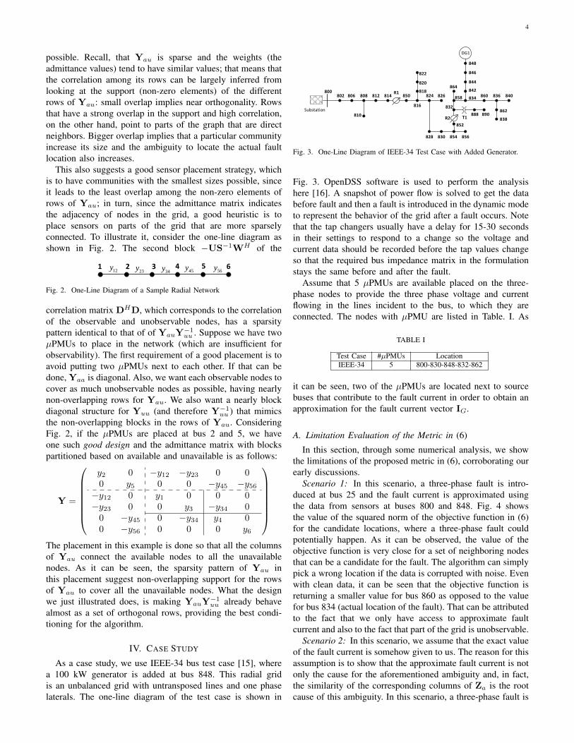
Fig. 3. One-Line Diagram of IEEE-34 Test Case with Added Generator.

Fig. 3. OpenDSS software is used to perform the analysishere [16]. A snapshot of power flow is solved to get the databefore fault and then a fault is introduced in the dynamic modeto represent the behavior of the grid after a fault occurs. Notethat the tap changers usually have a delay for 15-30 secondsin their settings to respond to a change so the voltage andcurrent data should be recorded before the tap values changeso that the required bus impedance matrix in the formulationstays the same before and after the fault.

Assume that 5 µPMUs are available placed on the three-phase nodes to provide the three phase voltage and currentflowing in the lines incident to the bus, to which they areconnected. The nodes with µPMU are listed in Table. I. As

TABLE I

Test Case #µPMUs LocationIEEE-34 5 800-830-848-832-862

it can be seen, two of the µPMUs are located next to sourcebuses that contribute to the fault current in order to obtain anapproximation for the fault current vector IG.

A. Limitation Evaluation of the Metric in (6)

In this section, through some numerical analysis, we showthe limitations of the proposed metric in (6), corroborating ourearly discussions.

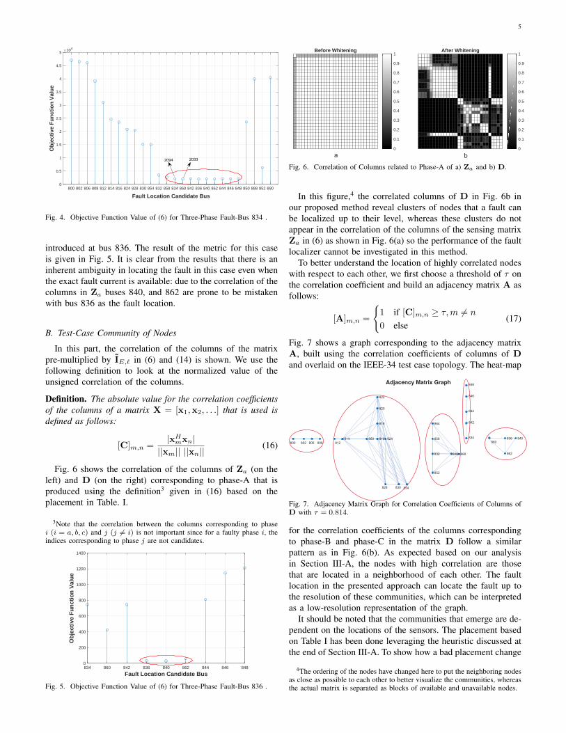
Scenario 1: In this scenario, a three-phase fault is intro-duced at bus 25 and the fault current is approximated usingthe data from sensors at buses 800 and 848. Fig. 4 showsthe value of the squared norm of the objective function in (6)for the candidate locations, where a three-phase fault couldpotentially happen. As it can be observed, the value of theobjective function is very close for a set of neighboring nodesthat can be a candidate for the fault. The algorithm can simplypick a wrong location if the data is corrupted with noise. Evenwith clean data, it can be seen that the objective function isreturning a smaller value for bus 860 as opposed to the valuefor bus 834 (actual location of the fault). That can be attributedto the fact that we only have access to approximate faultcurrent and also to the fact that part of the grid is unobservable.

Scenario 2: In this scenario, we assume that the exact valueof the fault current is somehow given to us. The reason for thisassumption is to show that the approximate fault current is notonly the cause for the aforementioned ambiguity and, in fact,the similarity of the corresponding columns of Za is the rootcause of this ambiguity. In this scenario, a three-phase fault is

5

0

0.5

1

1.5

2

2.5

3

3.5

4

4.5

5O

bje

ctiv

e F

un

ctio

n V

alu

e104

800 802 806 808 812 814 816 824 828 830 854 832 858 834 860 842 836 840 862 844 846 848 850 888 852 890

Fault Location Candidate Bus

20332094

Fig. 4. Objective Function Value of (6) for Three-Phase Fault-Bus 834 .

introduced at bus 836. The result of the metric for this caseis given in Fig. 5. It is clear from the results that there is aninherent ambiguity in locating the fault in this case even whenthe exact fault current is available: due to the correlation of thecolumns in Za buses 840, and 862 are prone to be mistakenwith bus 836 as the fault location.

B. Test-Case Community of Nodes

In this part, the correlation of the columns of the matrixpre-multiplied by IE,` in (6) and (14) is shown. We use thefollowing definition to look at the normalized value of theunsigned correlation of the columns.

Definition. The absolute value for the correlation coefficientsof the columns of a matrix X = [x1,x2, . . .] that is used isdefined as follows:

[C]m,n =|xH

mxn|||xm|| ||xn||

(16)

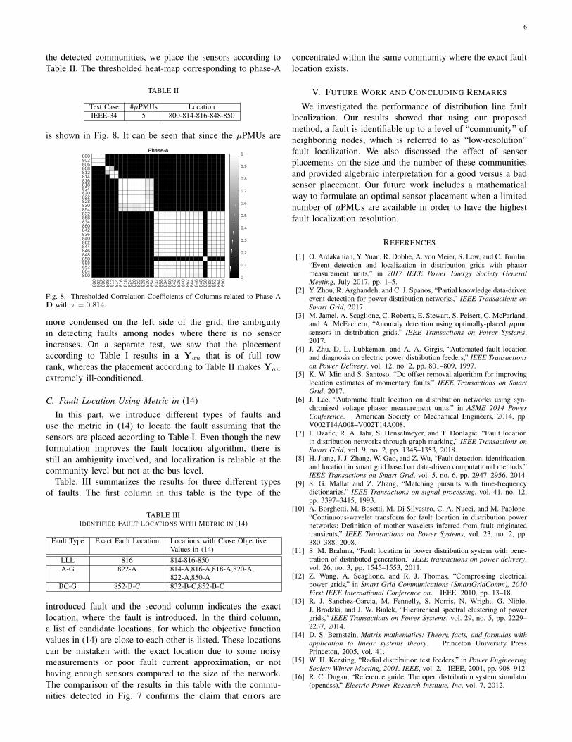
Fig. 6 shows the correlation of the columns of Za (on theleft) and D (on the right) corresponding to phase-A that isproduced using the definition3 given in (16) based on theplacement in Table. I.

3Note that the correlation between the columns corresponding to phasei (i = a, b, c) and j (j 6= i) is not important since for a faulty phase i, theindices corresponding to phase j are not candidates.

0

200

400

600

800

1000

1200

1400

Ob

ject

ive

Fu

nct

ion

Val

ue

834 860 842 836 840 862 844 846 848

Fault Location Candidate Bus

Fig. 5. Objective Function Value of (6) for Three-Phase Fault-Bus 836 .

Before Whitening

0

0.1

0.2

0.3

0.4

0.5

0.6

0.7

0.8

0.9

1After Whitening

0

0.1

0.2

0.3

0.4

0.5

0.6

0.7

0.8

0.9

1

a b

Fig. 6. Correlation of Columns related to Phase-A of a) Za and b) D.

In this figure,4 the correlated columns of D in Fig. 6b inour proposed method reveal clusters of nodes that a fault canbe localized up to their level, whereas these clusters do notappear in the correlation of the columns of the sensing matrixZa in (6) as shown in Fig. 6(a) so the performance of the faultlocalizer cannot be investigated in this method.

To better understand the location of highly correlated nodeswith respect to each other, we first choose a threshold of τ onthe correlation coefficient and build an adjacency matrix A asfollows:

[A]m,n =

{1 if [C]m,n ≥ τ,m 6= n

0 else(17)

Fig. 7 shows a graph corresponding to the adjacency matrixA, built using the correlation coefficients of columns of Dand overlaid on the IEEE-34 test case topology. The heat-map

Adjacency Matrix Graph

800 802 806 808 812 814 816

818

824

820

822

828 830 854

832

858 860

836 840

862

850

852

864

888 890

834

842

844

846

848

Fig. 7. Adjacency Matrix Graph for Correlation Coefficients of Columns ofD with τ = 0.814.

for the correlation coefficients of the columns correspondingto phase-B and phase-C in the matrix D follow a similarpattern as in Fig. 6(b). As expected based on our analysisin Section III-A, the nodes with high correlation are thosethat are located in a neighborhood of each other. The faultlocation in the presented approach can locate the fault up tothe resolution of these communities, which can be interpretedas a low-resolution representation of the graph.

It should be noted that the communities that emerge are de-pendent on the locations of the sensors. The placement basedon Table I has been done leveraging the heuristic discussed atthe end of Section III-A. To show how a bad placement change

4The ordering of the nodes have changed here to put the neighboring nodesas close as possible to each other to better visualize the communities, whereasthe actual matrix is separated as blocks of available and unavailable nodes.

6

the detected communities, we place the sensors according toTable II. The thresholded heat-map corresponding to phase-A

TABLE II

Test Case #µPMUs LocationIEEE-34 5 800-814-816-848-850

is shown in Fig. 8. It can be seen that since the µPMUs are

800

802

806

808

812

814

816

818

824

820

822

828

830

854

832

858

834

860

842

836

840

862

844

846

848

850

888

852

864

890

800802806808812814816818824820822828830854832858834860842836840862844846848850888852864890

Phase-A

0

0.1

0.2

0.3

0.4

0.5

0.6

0.7

0.8

0.9

1

Fig. 8. Thresholded Correlation Coefficients of Columns related to Phase-AD with τ = 0.814.

more condensed on the left side of the grid, the ambiguityin detecting faults among nodes where there is no sensorincreases. On a separate test, we saw that the placementaccording to Table I results in a Yau that is of full rowrank, whereas the placement according to Table II makes Yau

extremely ill-conditioned.

C. Fault Location Using Metric in (14)In this part, we introduce different types of faults and

use the metric in (14) to locate the fault assuming that thesensors are placed according to Table I. Even though the newformulation improves the fault location algorithm, there isstill an ambiguity involved, and localization is reliable at thecommunity level but not at the bus level.

Table. III summarizes the results for three different typesof faults. The first column in this table is the type of the

TABLE IIIIDENTIFIED FAULT LOCATIONS WITH METRIC IN (14)

Fault Type Exact Fault Location Locations with Close ObjectiveValues in (14)

LLL 816 814-816-850A-G 822-A 814-A,816-A,818-A,820-A,

822-A,850-ABC-G 852-B-C 832-B-C,852-B-C

introduced fault and the second column indicates the exactlocation, where the fault is introduced. In the third column,a list of candidate locations, for which the objective functionvalues in (14) are close to each other is listed. These locationscan be mistaken with the exact location due to some noisymeasurements or poor fault current approximation, or nothaving enough sensors compared to the size of the network.The comparison of the results in this table with the commu-nities detected in Fig. 7 confirms the claim that errors are

concentrated within the same community where the exact faultlocation exists.

V. FUTURE WORK AND CONCLUDING REMARKS

We investigated the performance of distribution line faultlocalization. Our results showed that using our proposedmethod, a fault is identifiable up to a level of “community” ofneighboring nodes, which is referred to as “low-resolution”fault localization. We also discussed the effect of sensorplacements on the size and the number of these communitiesand provided algebraic interpretation for a good versus a badsensor placement. Our future work includes a mathematicalway to formulate an optimal sensor placement when a limitednumber of µPMUs are available in order to have the highestfault localization resolution.

REFERENCES

[1] O. Ardakanian, Y. Yuan, R. Dobbe, A. von Meier, S. Low, and C. Tomlin,“Event detection and localization in distribution grids with phasormeasurement units,” in 2017 IEEE Power Energy Society GeneralMeeting, July 2017, pp. 1–5.

[2] Y. Zhou, R. Arghandeh, and C. J. Spanos, “Partial knowledge data-drivenevent detection for power distribution networks,” IEEE Transactions onSmart Grid, 2017.

[3] M. Jamei, A. Scaglione, C. Roberts, E. Stewart, S. Peisert, C. McParland,and A. McEachern, “Anomaly detection using optimally-placed µpmusensors in distribution grids,” IEEE Transactions on Power Systems,2017.

[4] J. Zhu, D. L. Lubkeman, and A. A. Girgis, “Automated fault locationand diagnosis on electric power distribution feeders,” IEEE Transactionson Power Delivery, vol. 12, no. 2, pp. 801–809, 1997.

[5] K. W. Min and S. Santoso, “Dc offset removal algorithm for improvinglocation estimates of momentary faults,” IEEE Transactions on SmartGrid, 2017.

[6] J. Lee, “Automatic fault location on distribution networks using syn-chronized voltage phasor measurement units,” in ASME 2014 PowerConference. American Society of Mechanical Engineers, 2014, pp.V002T14A008–V002T14A008.

[7] I. Dzafic, R. A. Jabr, S. Henselmeyer, and T. Donlagic, “Fault locationin distribution networks through graph marking,” IEEE Transactions onSmart Grid, vol. 9, no. 2, pp. 1345–1353, 2018.

[8] H. Jiang, J. J. Zhang, W. Gao, and Z. Wu, “Fault detection, identification,and location in smart grid based on data-driven computational methods,”IEEE Transactions on Smart Grid, vol. 5, no. 6, pp. 2947–2956, 2014.

[9] S. G. Mallat and Z. Zhang, “Matching pursuits with time-frequencydictionaries,” IEEE Transactions on signal processing, vol. 41, no. 12,pp. 3397–3415, 1993.

[10] A. Borghetti, M. Bosetti, M. Di Silvestro, C. A. Nucci, and M. Paolone,“Continuous-wavelet transform for fault location in distribution powernetworks: Definition of mother wavelets inferred from fault originatedtransients,” IEEE Transactions on Power Systems, vol. 23, no. 2, pp.380–388, 2008.

[11] S. M. Brahma, “Fault location in power distribution system with pene-tration of distributed generation,” IEEE transactions on power delivery,vol. 26, no. 3, pp. 1545–1553, 2011.

[12] Z. Wang, A. Scaglione, and R. J. Thomas, “Compressing electricalpower grids,” in Smart Grid Communications (SmartGridComm), 2010First IEEE International Conference on. IEEE, 2010, pp. 13–18.

[13] R. J. Sanchez-Garcia, M. Fennelly, S. Norris, N. Wright, G. Niblo,J. Brodzki, and J. W. Bialek, “Hierarchical spectral clustering of powergrids,” IEEE Transactions on Power Systems, vol. 29, no. 5, pp. 2229–2237, 2014.

[14] D. S. Bernstein, Matrix mathematics: Theory, facts, and formulas withapplication to linear systems theory. Princeton University PressPrinceton, 2005, vol. 41.

[15] W. H. Kersting, “Radial distribution test feeders,” in Power EngineeringSociety Winter Meeting, 2001. IEEE, vol. 2. IEEE, 2001, pp. 908–912.

[16] R. C. Dugan, “Reference guide: The open distribution system simulator(opendss),” Electric Power Research Institute, Inc, vol. 7, 2012.